Dirichlet Process Mixtures of Generalized Linear Models

Lauren Hannah lhannah@princeton.eduDepartment of Operations Research and Financial EngineeringPrinceton UniversityPrinceton, NJ 08544, USA

David Blei blei@cs.princeton.eduDepartment of Computer SciencePrinceton UniversityPrinceton, NJ 08544, USA

Warren Powell powell@princeton.edu

Department of Operations Research and Financial EngineeringPrinceton UniversityPrinceton, NJ 08544, USA

Editor: ????

Abstract

We propose Dirichlet Process-Generalized Linear Models (DP-GLM), a new method ofnonparametric regression that accommodates continuous and categorical inputs, and anyresponse that can be modeled by a generalized linear model. We prove conditions forthe asymptotic unbiasedness of the DP-GLM regression mean function estimate and givea practical example for when those conditions hold. Additionally, we provide Bayesianbounds on the distance of the estimate from the true mean function based on the number ofobservations and posterior samples. We evaluate DP-GLM on several data sets, comparingit to modern methods of nonparametric regression like CART and Gaussian processes.We show that the DP-GLM is competitive with the other methods, while accommodatingvarious inputs and outputs and being robust when confronted with heteroscedasticity.

1. Introduction

In this paper, we examine a Bayesian nonparametric solution to the general regressionproblem. The general regression problem models a response variable Y as dependent on aset of d-dimensional covariates X,

Y |X ∼ f(m(X)). (1)

In this equation, m(·) is a deterministic mean function, which specifies the conditional meanof the response, and f is a distribution, which characterizes the deviation of the responsefrom the conditional mean. In a regression problem, we estimate the mean function anddeviation parameters from a data set of covariate-response pairs (xi, yi)Ni=1. Given a newset of covariates xnew, we predict the response via its conditional expectation, E[Y |xnew].In Bayesian regression, we compute the posterior expectation of these computations, con-ditioned on the data.

1

Regression models have been a central focus of statistics and machine learning. The mostcommon regression model is linear regression. Linear regression posits that the conditionalmean is a linear combination of the covariates x and a set of coefficients β, and that theresponse distribution is Gaussian with fixed variance. Generalized linear models (GLMs)generalize linear regression to a diverse set of response types and distributions. In a GLM,the linear combination of coefficients and covariates is passed through a possibly non-linearlink function, and the underlying distribution of the response is in any exponential family.GLMs are specified by the functional form of the link function and the distribution ofthe response, and many prediction models, such as linear regression, logistic regression,multinomial regression, and Poisson regression, can be expressed as a GLM. Algorithms forfitting and predicting with these models are instances of more general-purpose algorithmsfor GLMs.

GLMs are a flexible family of parametric regression models: The parameters, i.e., thecoefficients, are situated in a finite dimensional space. A GLM strictly characterizes therelationship between the covariates and the conditional mean of the response, and im-plicitly assumes that this relationship holds across all possible covariates (McCullagh andNelder, 1989). In contrast, nonparametric regression models find a mean function in aninfinite dimensional space, requiring less of a commitment to a particular functional form.Nonparametric regression is more complicated than parametric regression, but can accom-modate a wider variety of response function shapes and allow for a response function thatadapts to the covariates. That said, nonparametric regression has its pitfalls: A methodthat is too flexible will over-fit the data; most current methods are tailored for specific re-sponse types and covariate types; and many nonparametric regression models are ineffectivefor high dimensional regression. See Hastie et al. (2009) for an overview on nonparametricregression and Section 1.1 below for a discussion of the current state of the art.

Here, we study Dirichlet process mixtures of generalized linear models (DP-GLMs), aBayesian nonparametric regression model that combines the advantages of generalized linearmodels with the flexibility of the nonparametric regression. With a DP-GLM, we modelthe joint distribution of the covariate and response with a DP mixture: the covariates aredrawn from a parametric distribution and the response is from a GLM, conditioned on thecovariates. The clustering effect of the DP mixture leads to an “infinite mixture” of GLMs,a model which effectively identifies local regions of covariate space where the covariatesexhibit a consistent relationship to the response. In combination, these local GLMs canrepresent arbitrarily complex global response functions. Note that the DP-GLM is flexiblein that the number of segments, i.e., the number of mixture components, is determined bythe observed data.

In a DP-GLM, the response function consists of piece-wise GLM models when condi-tioned on the component (i.e., covariate region).

A DP-GLM represents a collection of GLMs, one for each component, or region ofthe covariate space. In prediction, we are given a new covariate vector x, which inducesa conditional distribution over those components, i.e., over the coefficients that governthe conditional mean of the response. Integrating over this distribution, the predictedresponse mean is a weighted average of GLM predictions, each prediction weighted by theprobability that covariates x are assigned to its coefficients. Thus, the expected responsefunction E[Y |x] is not simply a piece-wise GLM. The sharp jumps between segments are

2

smoothed out by the uncertainty of the cluster assignment for the covariates that lie nearthe boundaries of the regions. (Furthermore, all of these computations are estimated in aBayesian way. We estimate and marginalize with respect to a posterior distribution overcomponents and parameters conditioned on a data set of covariate-response pairs.) Thismodel is a generalization of the Dirichlet process-multinomial logistic model of Shahbabaand Neal (2009).

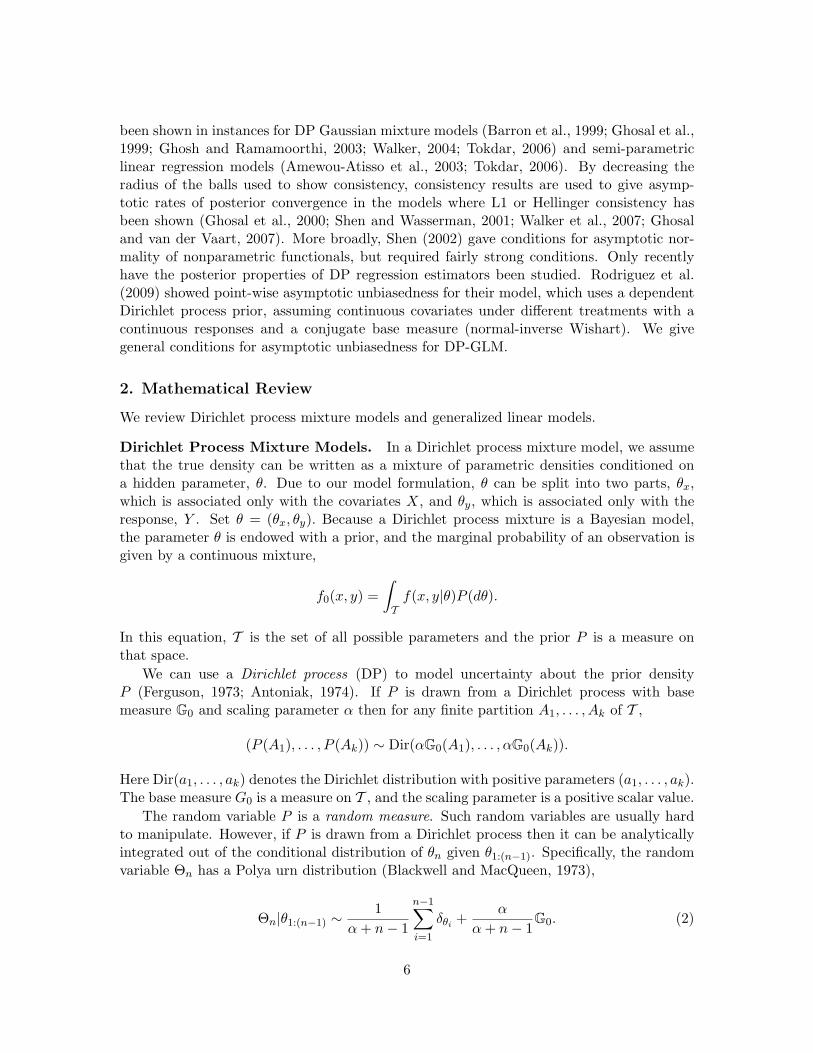
As an example, consider a simple linear regression setting with a single covariate. In thiscase, a GLM is a linear regression model and the DP mixture of linear regression modelsfinds multiple components, each of which is associated with a covariate mean and a set ofregression parameters. Conditioned on the region, the linear regression DP-GLM gives apiece-wise linear response function. But during prediction, the uncertainty surrounding theregion leads to a response function that smoothly changes at the boundaries of the region.This is illustrated in Figure 1, where we depict the maximum a posteriori (MAP) estimateof the piece-wise linear response and the smooth MAP response function E[Y |xnew].

The data in Figure 1 are heteroscedastic, meaning that the variance is not constantacross the covariate space. Most regression methods, including parametric methods, Gaus-sian process and SVM regression, assume that the variance is constant, or varies in a knownfashion. While these models can be modified to accommodate heteroscedasticity, DP-GLMaccommodates it natively by incorporating variance as a variable within each cluster.

In the remainder of this paper, we will show that DP-GLMs are an effective all-purposeregression technique that can balance the advantages of parametric modeling with the flex-ibility of nonparametric estimation. They readily handle high dimensional data, modelheteroscedasticity in the errors, and accommodate diverse covariate and response types.Moreover, we will show that DP-GLMs exhibit desirable theoretical properties, such as theasymptotic unbiasedness of the conditional expectation function E[Y |x].

The rest of this paper is organized as follows. In Section 2, we review Dirichlet processmixture models and generalized linear models. In Section 3, we construct the DP-GLM,describe its properties, and derive algorithms for posterior computation; in Section 4 we givegeneral conditions for unbiasedness and prove it in a specific case with conjugate priors.In Section 5 we compare DP-GLM and existing methods on three data sets with bothcontinuous covariates and response variables, one with continuous and categorical covariatesand a continuous response, and one with categorical covariates and a count response.

1.1 Related work

Nonparametric regression is a field that has received considerable study. Approaches to non-parametric regression can be broken into two general categories: frequentist and Bayesian.Bayesian methods assume a prior distribution on the set of all mean functions, whereasfrequentist methods do not. Frequentist nonparametric methods have comprised the bulkof the literature. Brieman et al. (1984) proposed classification and regression trees (CART),which partition the data and fit constant responses within the partitions. CART can beused with any type of data but produces a non-continuous mean function and is prone toover-fitting, particularly in situations with heteroscedasticity. Friedman (1991) proposedmultivariate adaptive regression splines (MARS), which selects basis functions with whichit builds a continuous mean function model. Locally polynomial methods (Fan and Gij-

3

0 100 200 300 400 500 600 700 800 9000

4,000

8,000

C`

Smoothed Estimate

0 100 200 300 400 500 600 700 800 9000

4,000

8,000

C`

Data Assigned to Clusters

0 100 200 300 400 500 600 700 800 9000

4,000

8,000

Multipole `

C`

Clusters

Figure 1: The underlying DP-GLM is the linear model described in equation (3). Thetop figure shows the smoothed regression estimate. The center figure shows thetraining data (blue) fitted into clusters, with the prediction given a single samplefrom the posterior, θ(i) (red). The bottom figure shows the underlying clusters(blue) centered around the mean ± one standard deviation; the fitted data (red)are plotted with each cluster. Data are from the cosmic microwave backgrounddata set of Bennett et al. (2003) that plots multipole moments against powerspectrum C`.

4

bels, 1996) calculate local polynomial coefficients via kernel weighting of the observations.Locally polynomial methods have attractive theoretical properties, such as unbiasedness atthe covariate boundaries, and often perform well. However, they are sensitive to kernelbandwidth and require dense sampling of the covariate space, which is often unrealistic inhigher dimensions. A number of techniques have been proposed for automatic bandwidthselection, in either a local or global form (Fan and Gijbels, 1995; Ruppert et al., 1995),sometimes combined with dimension reduction (Lafferty and Wasserman, 2008). Supportvector regression is an active field of research that uses kernels to map a high-dimensionalinput space into a lower dimensional feature space and fitting support vectors within thefeature space (see Smola and Scholkopf (2004) for a review). It can be sensitive to kernelchoice.

Gaussian process and Dirichlet process mixtures are the most common prior choices forBayesian nonparametric regression. Gaussian process priors assume that the observationsarise from a Gaussian process model with known covariance function form (see Rasmussenand Williams (2006) for a review). Since the size of the covariance function grows on theorder of the number of observations squared, much research has been devoted to sparse ap-proximations (Lawrence et al., 2003; Quinonero-Candela and Rasmussen, 2005; Snelson andGhahramani, 2006). Although Gaussian processes have been quite successful for regressionwith continuous covariates, continuous response and i.i.d. errors, other problem settingsoften require extensive modeling in order to use a GP prior.

We use a Dirichlet process mixture for regression; this in itself is not new. Escobarand West (1995) used a Gaussian kernel with a DP prior on the location parameter forBayesian density estimation; extension to the regression setting is trivial. West et al.(1994) and Muller et al. (1996) developed a model that uses a jointly Gaussian mixture overboth the covariates and response. The model is limited to a continuous covariate/responsesetting; the use of a fully populated covariance matrix makes the method impractical in highdimensions. More current methods have focused on mixing only over the response with aDP prior and correlating the distributions of the hidden response parameters according tosome function of the covariates. This has been achieved by using spatial processes or kernelfunctions of the covariates to link the local DPs (Griffin and Steel, 2006, 2007; Dunsonet al., 2007), or by using a dependent Dirichlet process prior (De Iorio et al., 2004; Gelfandet al., 2005; Duan et al., 2007; Rodriguez et al., 2009). These models can involve a largenumber of hidden variables or distributions and their complexity can pose difficulties fortheoretical claims about the resulting response estimators.

Dirichlet process priors have also been used in conjunction with GLMs. Mukhopadhyayand Gelfand (1997) and Ibrahim and Kleinman (1998) used a DP prior for the randomeffects portion of the the GLM; the model retains the linear relationship between the co-variates and response while allowing over dispersion to be modeled. Likewise, Amewou-Atisso et al. (2003) used a DP prior to model arbitrary symmetric error distributions in asemi-parametric linear regression model. Shahbaba and Neal (2009) proposed a model thatmixes over both the covariates and response, which are linked by a multinomial logisticmodel. The DP-GLM studied here is a generalization.

The asymptotic properties of models using Dirichlet process priors have not been wellstudied. Most current literature centers around consistency of the posterior density and itsrate of convergence to the true density. Weak, L1 (strong) and Hellinger consistency have

5

been shown in instances for DP Gaussian mixture models (Barron et al., 1999; Ghosal et al.,1999; Ghosh and Ramamoorthi, 2003; Walker, 2004; Tokdar, 2006) and semi-parametriclinear regression models (Amewou-Atisso et al., 2003; Tokdar, 2006). By decreasing theradius of the balls used to show consistency, consistency results are used to give asymp-totic rates of posterior convergence in the models where L1 or Hellinger consistency hasbeen shown (Ghosal et al., 2000; Shen and Wasserman, 2001; Walker et al., 2007; Ghosaland van der Vaart, 2007). More broadly, Shen (2002) gave conditions for asymptotic nor-mality of nonparametric functionals, but required fairly strong conditions. Only recentlyhave the posterior properties of DP regression estimators been studied. Rodriguez et al.(2009) showed point-wise asymptotic unbiasedness for their model, which uses a dependentDirichlet process prior, assuming continuous covariates under different treatments with acontinuous responses and a conjugate base measure (normal-inverse Wishart). We givegeneral conditions for asymptotic unbiasedness for DP-GLM.

2. Mathematical Review

We review Dirichlet process mixture models and generalized linear models.

Dirichlet Process Mixture Models. In a Dirichlet process mixture model, we assumethat the true density can be written as a mixture of parametric densities conditioned ona hidden parameter, θ. Due to our model formulation, θ can be split into two parts, θx,which is associated only with the covariates X, and θy, which is associated only with theresponse, Y . Set θ = (θx, θy). Because a Dirichlet process mixture is a Bayesian model,the parameter θ is endowed with a prior, and the marginal probability of an observation isgiven by a continuous mixture,

f0(x, y) =∫Tf(x, y|θ)P (dθ).

In this equation, T is the set of all possible parameters and the prior P is a measure onthat space.

We can use a Dirichlet process (DP) to model uncertainty about the prior densityP (Ferguson, 1973; Antoniak, 1974). If P is drawn from a Dirichlet process with basemeasure G0 and scaling parameter α then for any finite partition A1, . . . , Ak of T ,

(P (A1), . . . , P (Ak)) ∼ Dir(αG0(A1), . . . , αG0(Ak)).

Here Dir(a1, . . . , ak) denotes the Dirichlet distribution with positive parameters (a1, . . . , ak).The base measure G0 is a measure on T , and the scaling parameter is a positive scalar value.

The random variable P is a random measure. Such random variables are usually hardto manipulate. However, if P is drawn from a Dirichlet process then it can be analyticallyintegrated out of the conditional distribution of θn given θ1:(n−1). Specifically, the randomvariable Θn has a Polya urn distribution (Blackwell and MacQueen, 1973),

Θn|θ1:(n−1) ∼1

α+ n− 1

n−1∑i=1

δθi +α

α+ n− 1G0. (2)

6

(In this paper, lower case values refer to observed or fixed values, while upper case refer torandom variables.)

Equation (2) reveals the clustering property of the joint distribution of θ1:n: There ispositive probability that each θi will take on the value of another θj . This equation alsomakes clear the roles of α and G0. The unique values of θ1:n are drawn independently fromG0; the parameter α determines how likely Θn+1 is to be a newly drawn value from G0

rather than take on one of the values from θ1:n. G0 controls the distribution of the newcomponent.

In a DP mixture, θ is a latent parameter to an observed data point x,

P ∼ DP(αG0)Θi ∼ P

xi|θi ∼ f(· | θi).

Examining the posterior distribution of θ1:n given x1:n brings out its interpretation as an“infinite clustering” model. Because of the clustering property, observations are grouped bytheir shared parameters. Unlike finite clustering models, however, the number of groups israndom and unknown and, moreover, a new data point can be assigned to a new cluster thatwas not previously seen in the data. This model is amenable to efficient Gibbs samplingand algorithms (Neal, 2000; Blei and Jordan, 2005), and has emerged a powerful techniquefor flexible data analysis.

Generalized Linear Models. Generalized linear models (GLMs) build on linear regres-sion to provide a flexible suite of predictive models. While linear regression assumes aGaussian response, GLMs allow for any exponential family response by mapping a linearfunction of the covariates to the natural parameter of the response distribution. This embod-ies familiar models like logistic regression, Poisson regression, and multinomial regression.(Our review here is incomplete; See McCullagh and Nelder (1989) for a full discussion.)

A GLM assumes that a response variable Y is dependent on covariates X, with anexponential family distribution,

f(y|η) = exp(yη − b(η)a(φ)

+ c(y, φ)),

Here the canonical form of the exponential family is given, where a, b, and c are knownfunctions specific to the exponential family, φ is an arbitrary scale (dispersion) parameter,and η is the canonical parameter. The form of the exponential family (e.g. multinomial,Poisson, beta, Gaussian), called a random component, determines the form of the response,Y . A systematic component is included by setting the covariates to be a linear predictor ofthe canonical parameter,

η = Xβ.

The systematic and random components are combined via a link function g of the mean µ,where η = g(µ). It can be shown that b′(η) = µ, thereby connecting the linear predictor tothe canonical parameter, Xβ = g−1(b′(η)).

The canonical form is useful for discussion of GLM properties, but we use the meanform in the rest of this paper. For example, the canonical form of a Gaussian distribution,

7

setting η = µ is

f(y|η) = exp[yµ− µ2/2

σ2− y2

2σ2− log(σ

√2π)],

but we use the more familiar mean notation,

f(y|η) =1

σ√

2πexp

[− 1

2σ2(y − µ)2

].

3. Dirichlet Process Mixtures of Generalized Linear Models

We now turn to Dirichlet process mixtures of generalized linear models (DP-GLMs), a flex-ible Bayesian predictive model that places prior mass on a large class of response densities.Given a data set of covariate-response pairs, we describe Gibbs sampling algorithms forapproximate posterior inference and prediction. Theoretical properties of the DP-GLM aredeveloped in Section 4.

3.1 DP-GLM Formulation

In a DP-GLM, we assume that the covariates X are modeled by a mixture of exponential-family distributions, the response Y is modeled by a GLM conditioned on the inputs, andthat these models are connected by associating a set of GLM coefficients to each exponentialfamily mixture component. Let θ = (θx, θy) denote the bundle of parameters over X andY |X, and let G0 denote a base measure on the space of both. For example, θx might bea set of d-dimensional multivariate Gaussian location and scale parameters for a vector ofcontinuous covariates; θy might be a d+2-vector of reals for their corresponding GLM linearprediction coefficients, along with a nuisance term and a noise term for the GLM. The fullmodel is

P ∼ DP (αG0),(θx,i, θy,i)|P ∼ P,

Xi|θx,i ∼ fx(·|θx,i),Yi|xi, θy,i ∼ GLM(·|xi, θy,i).

The density fx describes the covariate distribution; the GLM for y depends on the form ofthe response (continuous, count, category, or others) and how the response relates to thecovariates (i.e., the link function).

The Dirichlet process prior on the parameters clusters the covariate-response pairs (x, y).When both are observed, i.e., in “training,” then the posterior distribution of this model willcluster data points according to near-by covariates that exhibit the same kind of relationshipto their response. When the response is not observed, its predictive expectation can beunderstood by clustering the covariates based on the training data, and then predicting theresponse according to the GLM associated with the covariates’ cluster.

Modeling the covariates with a mixture is not technically needed to specify a mixtureof GLMs. Many regression models use a DP mixture without explicitly mixing over thecovariates (De Iorio et al., 2004; Gelfand et al., 2005; Griffin and Steel, 2006, 2007; Dunsonet al., 2007; Duan et al., 2007; Rodriguez et al., 2009). The resulting models, however, are

8

often inflexible with respect to response/covariate type and have a high degree of complexity.Conversely, a full linear predictor required if we are modeling the covariates with a mixture.The inclusion of linear predictors in the DP-GLM greatly enhances the accuracy whileadding a minimal number of hidden variables.

Shahbaba and Neal (2009) use a specific version of DP-GLM for classification with amultinomial logit response function and continuous inputs, which they call the “DirichletProcess Multinomial Logistic Model” (dpMNL). We have fully generalized this model foruse in a variety of settings, including continuous multivariate regression, classification andPoisson regression.

We now give some examples of the DP-GLM that will be used throughout the rest ofthe paper.

Gaussian Model. In a simple case, the response has a Gaussian distribution, resultingin a linear regression within each cluster. That is,

fy(y|x, θi) =1

σi,y√

2πexp

− 12σ2

i,y

(y − βi,0 −d∑j=1

βi,jxj)2

.We assume continuous covariates modeled by Gaussian mixtures with mean µi,j and varianceσi, j2 for the jth dimension of the ith observation. The GLM parameters are the linearpredictor βi,0, . . . , βi,d and the noise coefficient σ2

i,y. Here, θx,i = (µi,1:d, σi,1:d) and θy,i =(βi,0:d, σi,y). The full model is,

P ∼ DP (αG0), (3)Θi = (µi,1:d, σi,1:d, βi,0:d, σi,y)|P ∼ P,

Xi,j |µi,j , σi,j ∼ N(µi,j , σ2i,j), j = 1, . . . , d,

Yi|xi, βi, σi,y ∼ N(βi,0 +d∑j=1

βi,jxi,j , σ2i,y).

Poisson Model. In a more complicated case, the response is count data. We modelthis with a Poisson distribution. We assume that the covariates are categorical; theseare modeled with multinomial mixtures with kj levels and parameters pi,j,1, . . . , pi,j,kj−1

in the jth dimension. Because the covariates are categorical, the linear predictor doesnot use the covariates themselves, but instead the indicators of covariate level. Definezi,j,` = 1xi,j= level ` for ` = 1, . . . , kj − 1. The hidden parameter is partitioned as follows:

θx,i = ((pi,1,1, . . . , pi,1,k1−1), . . . , (pi,d,1, . . . , pi,d,kd−1))

and

θy,i = (βi,0, βi,1,1:j1−1, . . . , βi,d,kd−1),

9

where βi,j,1:kj−1 is the set of linear predictors associated with zi,j . The full model is,

P ∼ DP (αG0),(pi,1:d, βi,0:d) ∼ P,Xi,j |pi,j,1:kj−1 ∼Multinomial(1, pi,j,1, . . . , pi,j,kj ), j = 1, . . . , d

Yi|xi, βi ∼1y!

exp

yβi,0 +

d∑j=1

kj−1∑`=1

βi,j,`zi,j,`

− exp

βi,0 +d∑j=1

kj−1∑`=1

βi,j,`zi,j,`

.The Role of G0. The choice of G0 is how prior knowledge about the hidden componentsis imparted, including the center and spread of their distribution. For example, supposethat the covariates X are as in the Gaussian model. The base measure on µ may be specifiedµ ∼ N(mµ, s

2µ). This would produce an accumulation of hidden parameters around mµ, with

large deviations unlikely. However, if µ ∼ Cauchy(mµ, b), the hidden parameters would stillbe centered around mµ, but the spread would be much greater.

Aside from prior knowledge considerations, the choice of base measure has computationalimplications. A conjugate base measure allows the analytical computation of many integralsthat involve the hidden parameters integrated with respect to the base measure. This cangreatly increase the efficiency of posterior sampling methods.

3.2 DP-GLM Regression

The DP-GLM is used in prediction problems. Given a collection of covariate-responsepairs (xi, yi)ni=1, our goal is to compute the expected response for a new set of covariates x.Conditional on the latent parameters θ1:n that generated the observed data, the expectationof the response is

E[Y |x, θ1:n] =α∫T E [Y |x, θ] fx(x|θ)G0(dθ) +

∑ni=1 E [Y |x, θi] fx(x|θi)

α∫T fx(x|θ)G0(dθ) +

∑ni=1 fx(x|θi)

. (4)

Since Y is assumed to be a GLM, the quantity E [Y |x, θ] is analytically available as afunction of x and θ.

The unobserved random variables Θ1:n are integrated out using their posterior distribu-tion given the observed data. Following the notation of Ghosh and Ramamoorthi (2003),let ΠP denote the DP prior on the set of hidden parameter measures, P . Let MT be thespace of all distributions over the hidden parameters. Since

∫T fy(y|x, θ)fx(x|θ)P (dθ) is a

density for (x, y), ΠP induces a prior on F , the set of all densities f on (x, y). Denote thisprior by Πf and define the posterior distribution,

Πfn (A) =

∫A

∏ni=1 f(Xi, Yi)Πf (df)∫

F∏ni=1 f(Xi, Yi)Πf (df)

,

where A ⊆ F . Define ΠPn similarly. Then the regression becomes

E[Y |x, (Xi, Yi)1:n] =1b

n∑i=1

∫MT

∫T

E[Y |x, θi]fx(x|θi)P (dθi)ΠPn (dP )

+α

b

∫T

E [Y |x, θ] fx(x|θ)G0(dθ), (5)

10

Algorithm 1: DP-GLM RegressionData: Observations (Xi, Yi)1:n, functions fx, fy, number of posterior samples M ,

query xResult: Mean function estimate at x, m(x)initialization;for m = 1 to M do

Obtain posterior sample θ(m)1:n |(Xj , Yj)1:n;

Compute E[Y |x, θ(m)1:n ];

end

Set m(x) = 1M

∑Mm=1 E[Y |x, θ(m)

1:n ];

where b normalizes the probability of Y being associated with the parameter θi,

b = α

∫Tfx(x|θ)G0(dθ) +

n∑i=1

∫MT

∫Tfx(x|θi)P (dθi)ΠP

n (dP ).

Equation (5) can also be written as

E [Y |x, (Xi, Yi)1:n] =∫ ∞−∞

yfn(y|x)dy, (6)

where fn(y|x) is the posterior predictive distribution after n observations,

fn(y|x) =

∫F f(y|x)

∏ni=1 f(Yi|Xi)Πf (df)∫

F∏ni=1 f(Yi|Xi)Πf (df)

. (7)

In this case, let f(y|x) = f(x, y)/(∫f(x, y)dy) and restrict Πf to place positive measure

only on the set f : f(x, y) > 0 for some y. Equation (5) is useful for implementation ofthe DP-GLM. The characterization in equation (6) is used to show theoretical properties,such as asymptotic unbiasedness.

Equations (5) and (6) are difficult to compute because they require integration over arandom measure. To avoid this problem, we approximate equation (5) by an average of MMonte Carlo samples of the expectation conditioned on θ1:n. This simpler computation isgiven in equation (8),

E[Y |x, (Xi, Yi)1:n] ≈ 1M

M∑m=1

E[Y |x, θ(m)

1:n

]. (8)

The regression procedure is given in Algorithm 1. We describe how to generate posteriorsamples (θ(m)

1:n )Mm=1 in Section 3.3.

11

Example: Gaussian Model. If we have the Gaussian model, equation (4) becomes

E[Y |x, θ1:n] =α

b

∫T

(β0 +d∑j=1

βjxj)d∏j=1

φσj (xj − µj)G0(dθ)

+1b

n∑i=1

(βi,0 +d∑j=1

βi,jxj)d∏j=1

φσi,j (xj − µi,j),

where

b = α

∫T

d∏j=1

φσj (xj − µj)G0(dθ) +n∑i=1

d∏j=1

φσi,j (xj − µi,j),

and

φσ(x) =1

σ√

2πexp

[− 1

2σ2x2

]is the Gaussian density at x with variance σ2.

An example of regression for a single covariate Gaussian model is shown earlier, inFigure 1. The bottom figure shows the mean and standard deviation for each clusterfrom one posterior sample. The middle figure shows how the training data are placed intoclusters and the top figure gives a smoothed estimate of the mean function for testing data.Clusters act locally to give an estimate of the mean function; in areas where there aremultiple clusters present, the mean function is generated by an average of the clusters.

Remark on Choice of G0. Equation (4) demonstrates one of the aspects of prior choice;it includes the term

α

∫Tfx(x|θ)G0(dθ),

which can be computed analytically if the base measure of θx is conjugate to fx(·|θ). If thisis not the case, integration must be performed numerically, which does not usually workwell in high dimensional spaces. Fortunately, if the covariate space is well-populated, thebase measure term is often inconsequential.

3.3 Posterior Sampling Methods

The above algorithm relies on samples of θ1:n|(Xi, Yi)1:n. We use Markov chain Monte Carlo

(MCMC), specifically Gibbs sampling, to obtainθ

(m)1:n |(Xi, Yi)1:n

Mm=1

. Gibbs sampling

has a long history of being used for DP mixture posterior inference (see Escobar (1994);MacEachern (1994); Escobar and West (1995) and MacEachern and Muller (1998) for foun-dational work; Neal (2000) provides a modern treatment and state of the art algorithms).While DP mixtures were proposed in the 1970’s, they did not become computationallyfeasible until the mid-1990’s, with the advent of these MCMC methods.

Gibbs sampling uses the known conditional distributions of the hidden variables ina sequential manner to generate a Markov chain that has the unknown joint distribu-tion of the hidden parameters as its ergodic distribution. That is, the state variable φiassociated with observation (Xi, Yi) is drawn given that the rest of the state variable,

12

(φ1, . . . , φi−1, φi+1, . . . , φn), is fixed. θi is selected according to the Polya urn scheme ofequation (2).

The composition of the state variable is determined by the base measure, G0. If G0

is conjugate to the model, the hidden parameters can be integrated out of the posterior,leaving only a cluster number as a state variable. Non-conjugate base measures require thatthe state variable for (Xi, Yi) is the hidden mixture parameter, θi.

To obtain posterior samples, the state variables are updated in a sequential mannerover many iterations. Samples are the observed state variables. Two main problems arisebecause the samples are drawn from a Markov chain. First, successive observations are notindependent. Second, observations should be drawn from the posterior distribution onlyonce the Markov chain has reached its ergodic distribution. The first problem is usuallyapproached by sampling in a pulsed manner; e.g., after sampling, the next sample will occur10 iterations later. The second problem is much more difficult.

Since we are not able to compute the full posterior distribution, we must rely on samplesdrawn from the MCMC to infer whether convergence has been reached. First, we try toobtain a relatively “good” starting point for the state variable to speed mixing; this isoften done through a priori information or a mode estimate. Then to minimize the impactof starting position, we discard the early iterations of the sampler in a burn-in period.Further precautions include checking whether the log likelihood of the posterior has “leveledoff” or computing parameter variation estimates based on between- and within- sequencevariances (Brooks and Gelman, 1998). For a full discussion of convergence assessment, seeGelman et al. (2004).

A simple Gibbs sampler for a non-conjugate base measure is given in Algorithm 2.

Other Posterior Sampling Methods. MCMC is not the only way to sample from theposterior. Blei and Jordan (2005) apply variational inference methods to Dirichlet processmixture models. Variational inference methods use optimization to create a parametricdistribution close to the posterior from which samples can be drawn. Variational inferenceavoids the issue of determining when the stationary distribution has been reached, but lackssome of the convergence properties of MCMC. Fearnhead (2004) uses a particle filter togenerate posterior samples for a Dirichlet process mixture. Particle filters also avoid havingto reach a stationary distribution, but the large state vectors created by non-conjugate basemeasures and large data sets can lead to collapse.

Hyperparameter Sampling. Hyperparameters, such as α and the parametric compo-nents of G0, can be sampled via Gibbs sampling. For our numerical experiments below (seeSection 5), we placed a gamma prior on α and resampled every five iterations. Samplingfor hyperparameters associated with G0 varied with the choice of G0.

3.4 The Conditional Distribution of DP-GLM

We have formulated the DP-GLM and given an algorithm for posterior inference and predic-tion. Finally, we explore precisely the type of model that the DP-GLM produces. Considerthe distribution f(y|x) for a fixed x under DP-GLM. This is also a mixture model with

13

Algorithm 2: MCMC Gibbs Sampling for the DP-GLM Posterior with Non-Conjugate Base Measures

Data: Observations (Xi, Yi)1:n, initial MCMC state θ(1)1:n, number of posterior

samples M , lag time L, MC convergence criteriaResult: Posterior sample (θ(m)

1:n )Mm=1

initialization;Set ` = 0, i = 1, m = 1;while m ≤M do

for j = 1 to n doDraw θ

(m+1)i |θ(m)

1 , . . . , θ(m)j−1, θ

(m)j+1, . . . , θ

(m)n , (Xi, Yi)1:n;

Set m = m+ 1;endif Convergence criteria satisfied then

if remainder(`, L) = 0 thenSet θ(m)

1:n = θ(m)1:n ;

Set i = i+ 1;endSet ` = `+ 1;

endend

hidden parameters,

f(y|x) =∞∑i=1

fy(y|x, θy)p(θy|x).

Usually the full set of hidden parameters can be collapsed into a smaller set only associatedwith y, θy. In general, for a fixed x, θy alone does not have a Dirichlet process prior.

To see why we lose the Dirichlet process prior for the conditional distribution, we workwith the Poisson random measure construction of a Dirichlet process (Pitman, 1996). First,we construct a Poisson random measure representation for the hidden parameters of thefull model. We then fix x and use a transition kernel generated by the DP-GLM modelto move the process from (θ, p) to (θy, q). This induces a new Poisson random measure.The parameter θy is usually just a subset of θ, but q is generated by weighting p by somefunction of θ and x. It is in this change of weights that the Dirichlet process prior is lost.We compute a necessary and sufficient condition under which the resulting Poisson randommeasure also characterizes a Dirichlet process.

Theorem 1 (Pitman (1996)) Let Γ(1) > Γ(2) > . . . be the points of a Poisson randommeasure on (0,∞) with mean measure α e

−p

p dp. Put

Gi = Γ(i)/Λ,

where Λ =∑

i Γ(i) and define

F =∞∑i=1

GiδΘi , (9)

14

where Θi are i.i.d. µ(dθ)g0(dθ) = G0(dθ), independent also of the Γ(i). Then, F is aDirichlet process with base measure (αG0).

The pairs (Θi,Γ(i)) form a Poisson random measure on T × (0,∞) with mean measure

ν(dθ, dp) = g0(θ)αe−p

pµ(dθ)dp. (10)

Now consider the induced mixture model on the y component. If the joint model has aDirichlet process prior, then

∞∑i=1

fy(y|θi, x)p(θi|x) =∞∑i=1

fy(y|θi, x)p(x|θi)p(θi)

p(x)

=∞∑i=1

fy(y|θ(i), x)p(x|θ(i))Γ(i)

Λ∫p(x|θ)F (dθ)

=∞∑i=1

fy(y|θ(i), x)p(x|θ(i))Γ(i)∑∞i=1 p(x|θ(i))Γ(i)

. (11)

The conditional measure on the hidden parameters in equation (11) has the same form as themeasure in equation (9) where Γ(i) is replaced by p(x|θ(i))Γ(i) and Λ by

∑∞i=1 p(x|θ(i))Γ(i).

When we shift from the overall model to the conditional model, two mappings occur.The first maps θ to θy, where θy is usually just a subset of the hidden parameter vector θ.The second maps p to q, and usually depends on both p and θ. We will represent these bya transition kernel, Kx(θ, p; dθy, dq). For instance, if we have the Gaussian model, then

Kx(θ, p; dθy, dq) = δβ(β)δσy(σy)δpQdi=1 φσi (xi−µi)

(q)dβdσydq, (12)

where φσ(x) is the Gaussian pdf with standard deviation σ evaluated at x and δy(x) is theDirac measure with mass at y. The transition is deterministic.

Using the transition kernel, we can calculate a mean measure ν(dθy, dq) for the inducedPoisson random measure,

ν(dθy, dq) =∫T

∫(0,∞)

µ(dθ) dpg0(θ)αe−p

pKx(θ, p; dθy, dq).

To remain as a Dirichlet process prior, ν must have the same form as equation (10),where g0(θ) is allowed to be flexible, but the measure on the weights must have the formα q−1e−qdq. In the following Theorem, we give a necessary and sufficient condition for this.

Theorem 2 Fix x. Let (Θ,Γ) have a Dirichlet process prior with base measure αG0 andlet (Θy,Υ) be the parameters and weights associated with the conditional mixture. Then,the prior on (Θy,Υ) is a Dirichlet process if and only if for every λ > 0,∫

Tµ(dθ)g0(θ)

∫(0,∞)

dpe−p

p

∫(0,∞)

Kx(θ, p; dθy, dq)(

1− e−λq)

= νθ(dθy) log (1 + λ) .

15

Proof Let h(q) = 1− e−λq, then set∫T

∫(0,∞)

µ(dθ) dpg0(θ)αe−p

pKx(θ, p; dθy, dq)h(q) = ν(dθy, dq)h(q),

and integrate over q. Like a Laplace transform, the expectation of h uniquely characterizesthe distribution.

Example: Gaussian Model. We use Theorem 2 to check the mean measure of theconditional distribution. For the transition kernel given in equation (12),∫

Tµ(dθ)g0(θ)

∫(0,∞)

dpe−p

p

∫(0,∞)

Kx(θ, p; dθy, dq)(

1− e−λq)

=∫Tµ(dθ)g0(θ)

∫(0,∞)

dq

(exp (−q/f(θ))− exp (−q/f(θ)(1 + λf(θ)))

q/f(θ)

),

= dβdσyg0(β, σy)∫Tf(θ) log(1 + λf(θ))µ(dθ)g0(µ1:d, σ1:d),

where f(θ) =∏di=1 φσi(xi−µi). Notice that the f(θ) term has slipped into the log function,

making q dependent on θ and, therefore, the prior on the conditional parameters not aDirichlet process.

Practically, this construction tells us that the most efficient means of sampling theconditional posterior distribution is via the joint posterior distribution. Sampling the jointdistribution allows us to use the structure of the Dirichlet process (either the stick-breakingconstruction of Sethuraman (1994) or the Polya urn posterior). The conditional posteriormay have fewer hidden variables, but it lacks the DP mathematical conveniences.

4. Asymptotic Unbiasedness of the DP-GLM Regression Model

We cannot assume that the mean function estimate computed with the DP-GLM will beclose to the true mean function, even in the limit. Diaconis and Freedman (1986) give anexample of a location model with a Dirichlet process prior where the estimated location canbe bounded away from the true location, even when the number of observations approachesinfinity. We want to assure that DP-GLM does not end up in a similar position.

Traditionally, an estimator is called unbiased if the expectation of the estimator overthe observations is the true value of the quantity being estimated. In the case of DP-GLM,that would mean for every x ∈ A and every n > 0,

Ef0 [EΠ[Y |x, (Xi, Yi)ni=1]] = Ef0 [Y |x],

where A is some fixed domain, EΠ is the expectation with respect to the prior Π and Ef0is the expectation with respect to the true distribution.

Since we use Bayesian priors in DP-GLM, we will have bias in almost all cases (Gelmanet al., 2004). The best we can hope for is asymptotic unbiasedness, where as the number

16

of observations grows to infinity, the mean function estimate converges to the true meanfunction. That is, for every x ∈ A,

EΠ[Y |x, (Xi, Yi)ni=1]→ E[Y |x] as n→∞.

Diaconis and Freedman (1986) give an example for a location problem with a DP prior wherethe posterior estimate was not asymptotically unbiased. Extending that example, it followsthat estimators with DP priors do not automatically receive asymptotic unbiasedness.

The question is under which circumstances does the DP-GLM escape the Diaconis andFreedman (1986) trap and have asymptotic unbiasedness. To show that the DP-GLM isasymptotically unbiased, we use equation (6) and show that∣∣∣Ef0 [Y |x]− Efn [Y |x]

∣∣∣→ 0

in an appropriate manner as n → ∞, where Ef [·] means “expectation under f” and fn isthe posterior predictive density, given in equation (7).

We show asymptotic unbiasedness through consistency. It is the idea that, given anappropriate prior, as the number of observations goes to infinity the posterior distributionaccumulates in neighborhoods arbitrarily “close” to the true distribution. Consistency de-pends on the model, the prior and the true distribution. Consistency gives the conditionthat, if the posterior distribution accumulates in weak neighborhoods (sets of densities un-der which the integral of all bounded, continuous functions is close to the integral under thetrue density), the posterior predictive distribution converges weakly to the true distribution(meaning that the posterior predictive distribution is in all weak neighborhoods of the truedistribution). Weak convergence of measure is not sufficient to show convergence in expec-tation; uniform integrability of the random variables generated by the posterior predictivedensity is also required. When weak consistency is combined with uniform integrability,asymptotic unbiasedness is achieved.

In this section, we first review consistency and related topics in subsection 4.1. Usingthis basis, in subsection 4.2 we state and prove Theorem 9, which gives general conditionsunder which the mean function estimate given by DP-GLM is asymptotically unbiased. Insubsection 4.3, we use Theorem 9 to show DP-GLM with conjugate priors produces anasymptotically unbiased estimate for the Gaussian model and related models.

4.1 Review of Consistency and Related Topics

Let F0 be the true distribution. For convenience in the integral notation, we assume thatall densities are absolutely continuous with respect to the Lebesgue measure, but that neednot be the case (for example, a density may be absolutely continuous with respect to acounting measure). Let Ef [Y ] denote

∫yf(y)dy, the expectation of Y under the density f ,

let Ω be the outcome space for (Xi, Yi)∞i=1, let F∞0 be the infinite product measure on thatspace, and let fn(x) be the posterior predictive density given observations (Xi, Yi)ni=1.

Weak consistency, and uniform integrability form the basis of convergence for this prob-lem. Weak consistency, uniform integrability and related topics are outlined below.

First, we define weak consistency and show that weak consistency of the prior impliesweak convergence of the posterior predictive distribution to the true distribution.

17

Definition 3 A weak neighborhood U of f0 is a subset of

V =f :∣∣∣∣∫ g(x)f(x)dx−

∫g(x)f0(x)dx

∣∣∣∣ < ε for all bounded, continuous g.

A weak neighborhood of f0 is a set of densities defined by the fact that integrals of all “wellbehaving functions,” i.e. bounded and continuous, taken with respect to the densities inthe set are within ε of those taken with respect to f0. This definition of “closeness” caninclude some densities that vary greatly from f0 in sufficiently small areas.

Definition 4 Π(·|(Xi, Yi)1:n) is said to be weakly consistent at f0 if there is a Ω0 ⊂ Ωsuch that P∞F0

(Ω0) = 1 and ∀ω ∈ Ω0, for every weak neighborhood U ,

Π(U |(Xi, Yi)1:n(ω))→ 1

for all weak neighborhoods of f0.

Weak consistency means that the posterior distribution gathers in the weak neighborhoodsof f0.

Let fn ⇒ f denote that fn converges to f weakly. That is,∫g(x)fn(x)dx→

∫g(x)f(x)dx

for all bounded, uniformly continuous functions g.The following proposition shows that weak consistency of the prior induces weak con-

vergence of the posterior predictive distribution, fn, as described in equation (7), to thetrue distribution, f0.

Proposition 5 If Πf (·|(Xi, Yi)1:n) is weakly consistent at f0, then fn ⇒ f0, almost surelyP∞F0

.

Proof Let U be a weak neighborhood of f0. Let g be bounded and continuous. Then,∣∣∣∣∫ g(y)fn(y|x)dy −∫g(y)f0(y|x)dy

∣∣∣∣ =∣∣∣∣∫ g(y)

∫Ff(y|x)Πf

n(df)−∫g(y)f0(y|x)dy

∣∣∣∣ ,≤∣∣∣∣∫U

∫g(y)f(y|x)dy −

∫g(y)f0(y|x)dy

∣∣∣∣+∣∣∣∣∫UC

∫g(y)f(y|x)dy

∣∣∣∣≤ ε+ o(1).

Since weak consistency implies weak convergence of the posterior predictive distributionto the true distribution, we need to show weak consistency. To do this, we first use theKullback-Leibler (KL) divergence between two densities f and g, K(f, g), where

K(f, g) =∫

Rdf(x) log

(f(x)g(x)

)dx.

18

Next, consider neighborhoods of densities where the KL divergence from f0 is less than εand define Kε = g : K(f0, g) < ε . If Πf puts positive measure on these neighborhoods forevery ε > 0, then we say that Πf is in the K-L support of f0.

Definition 6 For a given prior Πf , f0 is in the K-L support of Πf if ∀ε > 0, Πf (Kε(f0)) >0; this is denoted by f0 ∈ KL(Πf ).

A theorem by Schwartz (1965), as modified by Ghosh and Ramamoorthi (2003), providesa simple way to show weak posterior consistency using the idea of K-L support.

Theorem 7 (Schwartz (1965)) Let Πf be a prior on F . If f0 is in the K-L support ofΠf , then the posterior is weakly consistent at f0.

Weak consistency alone does not prove convergence of Efn [Y |x] to Ef0 [Y |x]. Let (Fn)∞n=1

be the filtration generated by the observations where Fn = σ((Xi, Yi)ni=1) and σ is theminimal σ-algebra. The sequence of random variables (Y |x,Fn)∞n=1 needs to be uniformlyintegrable to ensure convergence of Efn [Y |x] to Ef0 [Y |x] for a specific x. This gives point-wise convergence of the conditional expectation.

Definition 8 A set of random variables X1, X2, . . . is uniformly integrable if

ρ(α) = supn

E[|Xn|1|Xn|>α

]→ 0,

as α→∞.

This definition is often hard to check, so we rely on a well known sufficient condition foruniform integrability (Billingsley, 2008). If there exists an ε > 0 such that,

supn

E[|Xn|1+ε

]<∞,

then the sequence (Xn)n≥1 is uniformly integrable.We now have the necessary concepts to discuss the asymptotic unbiasedness of DP-GLM

regression.

4.2 Asymptotic Unbiasedness of the DP-GLM Regression Model

In this subsection we give a general result for the asymptotic unbiasedness of the DP-GLMregression model. We do this by showing uniform integrability of the conditional expec-tations in Lemma 11. We show uniform integrability by demonstrating that the posteriorpredictive densities, fn(y|x) are martingales with respect to Fn in Lemma 10. The martin-gale property used to create the positive martingale Efn

[|Y |1+ε|x

], which is used to show

uniform integrability of (Y |x,Fn)∞n=1. We are now ready to state the main theorem.

Theorem 9 Fix x. Let Πf be a prior on F . If

(i) Πf is in the K-L support of f0(y|x),

(ii)∫|y|f0(y|x)dy <∞, and

19

(iii) there exists an ε > 0 such that∫ ∫|y|1+εfy(y|x, θ)G0(dθ) <∞,

then Efn [Y |x]→ Ef0 [Y |x] almost surely PF∞0 .

The conditions of Theorem 9 must be checked for the problem (f0) and prior (Πf ) pair, whichwe do for the Gaussian model in subsection 4.3. Condition (i) assures weak consistency ofthe posterior. Condition (iii) ensures that ΠP

P :

∫ ∫|y|1+εfy(y|x, θ)P (dθ)

= 1, meaning

that the random variable with the density f is almost surely uniformly integrable. Together,conditions (ii) and (iii) assure that there will always be a finite conditional expectation andthat it is uniformly integrable.

To prove Theorem 9, we first show the integrability of the random variables generatedby the posterior predictive distribution via martingale methods. While traditional mixturesof Gaussian densities are always uniformly integrable, this is not always the case when thelocation parameters are chosen according to an underlying distribution. That is, a priorwith sufficiently heavy tails may not produce a uniformly integrable mixture. We begin byshowing that the distribution fn(y|x) is a martingale.

The following Lemma is found in Nicoleris and Walker (2006):

Lemma 10 The predictive density fn(y|x) at the point (y, x) is a martingale with respectto the filtration (Fn)n≥0.

Lemma 10 is useful for constructing other martingales, such as Efn [|Y |1+ε|x]. We usethese martingales to show uniform integrability of the random variables generated by theposterior predictive distribution.

Lemma 11 Suppose that conditions (ii) and (iii) of Theorem 9 are satisfied. Then,

supn

Efn [|Y |1+ε|x] <∞.

Proof Efn [|Y |1+ε|x] is a positive martingale with respect to (Fn)n≥0 and conditions (ii)−(iii) assure that this quantity will always exist. Since it is a positive martingale, it willalmost surely converge to a finite limit. Therefore,

supn

Efn [|Y |1+ε|x] <∞

almost surely PF∞0 .

Using Lemma 11, the proof of Theorem 9 follows.Proof [Proof of Theorem 9] By Theorem 7, condition (i) implies weak consistency of theprior. Proposition 5 states that weak consistency implies weak convergence of the posteriorpredictive density. Conditions (ii) and (iii) imply uniform integrability of that density,which taken along with weak convergence give convergence of the expectation.

20

Showing that the conditions of Theorem 9 are satisfied requires some effort. In the nextsubsection we demonstrate that they are satisfied for the Gaussian model with a conjugatebase measure.

4.3 Asymptotic Unbiasedness of DP-GLM for a Gaussian Model with aConjugate Base Measure

In Theorem 9, the most difficult condition to satisfy is condition (i), which requires that theprior of the conditional distribution be weakly consistent. This subsection shows that theGaussian model with a conjugate base measure satisfies condition (i). Additionally, theyalso satisfy condition (iii), resulting in asymptotic unbiasedness so long as the true meanfunction actually exists.

To reach this conclusion, we first explore how the prior on the joint distribution isrelated to the prior on the conditional distribution. It turns out that KL divergence for theconditional prior is very similar to the KL divergence of the joint prior. Next, we modifythe work of Tokdar (2006), which gives weak consistency conditions for a single-dimensionallocation-scale mixture of Gaussians where the hidden parameters have a Dirichlet processprior. We do this by mapping the DP-GLM Gaussian model to a model that only hasa location-scale response and show that the prior on these parameters is still a Dirichletprocess in Lemma 12. Then we extend the work of Tokdar (2006) to give weak consistencycriteria for the prior on a multidimensional location-scale mixture in Theorem 14. Finally,we show that a conjugate base measure satisfies Theorem 14.

Weak Consistency Theorems. Fix x. Using Theorem 7, weak consistency for a givenf0 and prior Πf can be proven by showing that for an arbitrary ε > 0, the set f :f satisfies Equation 13 has strictly positive measure under Πf , where∫ ∞

−∞f0(y|x) log

f0(y|x)f(y|x)

dy < ε. (13)

Since ΠP is defined on the hidden parameters of the joint distribution of f(x, y) and notthe conditional f(y|x), we need to express equation (13) using the joint distribution. Letf(x) =

∫f(x, y)dy. Then,∫ ∞−∞

f0(y|x) logf0(y|x)f(y|x)

dy =∫ ∞−∞

f0(x, y)f0(x)

(log

f0(x, y)f(x, y)

+ logf(x)f0(x)

)dy,

= logf(x)f0(x)

+1

f0(x)

∫ ∞−∞

f0(x, y) logf0(x, y)f(x, y)

dy.

To give conditions for weak consistency, we build a series of Lemmas that are similarto those of Tokdar (2006). That work gives conditions for the weak consistency of a one-dimensional continuous density with a Dirichlet process prior on a location-scale mixture.We extend these results to our setting. First, we show that for a fixed x the DP prior on thelocation, scale and slopes of DP-GLM induces a DP prior on a location-scale mixture. Thenwe approach the problem in the same manner as Tokdar (2006) and modify the Lemmasused for a multidimensional setting. Lemma 13 gives a tail condition that, if satisfied,

21

guarantees weak consistency. Theorem 14 constructs a prior that satisfies Lemma 13 byplacing restrictions on the DP base measure, G0.

DP-GLM does not have the traditional location-scale format used in Muller et al. (1996),Ghosal et al. (1999) and Tokdar (2006), but instead has conditional response densityφσy(y − β0 −

∑di=1 βixi), where φσ(x) is the Gaussian probability density function with

standard deviation σ evaluated at x. For fixed x, however, we can introduce the locationparameter η = β0 + β1x1 + · · · + βdxd. Lemma 12 shows the parameters (η, σy, µ1:d, σ1:d)also have a Dirichlet process prior. Similar mappings also have Dirichlet process priorsbecause they change only the base measure of the hidden parameters, G0, not the weightsassociated with each component. Let ΠP be the original prior and ΠP be the induced prioron P (η, σy, µ1:d, σ1:d).

Lemma 12 For a fixed x, let η = β0 + β1x1 + · · · + βdxd. If ΠP ∼ DP (α,G0), thenΠP ∼ DP (α, G0), where

G0(A1 ×A2 ×A3) =∫

Rd+1

1A1 (η) G0(dβ0, . . . , dβd, A2, A3).

The proof is in the Appendix. This lemma allows us to follow the methods of Tokdar (2006)closely by changing our parameters into the same location-scale mixtures. We need onlyextend the theorems of Tokdar (2006) to multiple dimensional settings.

The following lemma uses a tail condition on the KL divergence that, if satisfied, showsthat the true density is in the KL support of the prior. In order to state the density f interms of P , we use f = φd+1∗P to denote the convolution of the d+1 dimensional Gaussianpdf with the measure P (η, σy, µ1:d, σ1:d).

Lemma 13 Suppose that f0 ∈ F and ΠP satisfies the following properties: for any 0 <τ < 1 and any ε > 0, there exists a set A and a y0 > 0 such that,

i) f0(x) > 0,

ii) there exists a closed hypercube D ⊂ Rd such that x ∈ int(D) and∫D×R

f0(x, y) log f0(x, y)dxdy <∞,

iii) ΠP (A) > 1− τ , and

iv) for any f = φd+1 ∗ P with P ∈ A,∫|y|>y0

f0(x, y) logf0(x, y)f(x, y)

dy < ε.

Then, f0(y|x) ∈ KL(Πf ).

The proof is in the Appendix. Now, we construct conditions for which Lemma 13 holds.This is done mainly by constructing tail conditions on the base measure for the responselocation-scale parameters, G0,y. For convenience, we assume that the base measure on thecovariate parameters, G0,x is independent of G0,y.

22

Theorem 14 Fix x. Let f0 be a density on Rd+1 satisfying,

i) f0(x) > 0,

ii) there exists a closed hypercube D ⊂ Rd such that x ∈ int(D) and∫D×R

f0(x, y) log f0(x, y)dxdy <∞,

iii) there exists γ ∈ (0, 1) such that∫|y|γf0(x, y)dy <∞.

Further assume that G0,y is independent of G0,x. Assume that G0,x puts positive density onall possible hidden parameter values. Assume that there exist σ0 > 0, 0 < ν < γ, ψ > ν andb1, b2 > 0 such that for large y > 0,

iv) max

G0,y

([y − σ0y

γ/2,∞)× [σ0,∞)), G0,y

([0,∞)× (y1−γ/2,∞)

)≥ b1y−ν ,

v) G0,y ((−∞, y)× (0, exp[|y|γ − 1/2])) > 1− b2|y|−ψ,

and for large y < 0,

iv′) max

G0,y

((−∞, y + σ0|y|γ/2]× [σ0,∞)

), G0,y

((−∞, 0]× (|y|1−γ/2,∞)

)≥ b1|y|−ν ,

v′) G0,y ((y,∞)× (0, exp[|y|γ − 1/2])) > 1− b2|y|−ψ,

then f0(y|x) ∈ KL(Πf ).

The proof is in the Appendix. The conditions v) and v′) require that the tails of G0,y

not decay faster than a polynomial rate for σy. Now that we have conditions under whichthe KL support condition is satisfied, we can apply them to the Gaussian model with aconjugate base measure.

Asymptotic Unbiasedness for Conjugate Base Measures. We use the results ofTheorem 9 and Theorem 14 to show asymptotic unbiasedness of conjugate base measuresfor the Gaussian model. The conjugate base measure G0 for the covariates of the location-scale Gaussian mixture model is

σ−2i ∼ Gamma(ri, λi), i = 1, . . . , d,

µi|σi ∼ N(νi, ξi σ2i ), i = 1, . . . , d.

Define both G0,x and G0,x in that manner. In either of these cases, for a fixed x we cansatisfy conditions i) and ii) of Theorem 14.

The matter of G0,y is somewhat more complicated; Tokdar (2006) shows that if G0,y,the base distribution for the location-scale mixture of the y component satisfies

σ−2y ∼ Gamma(ry, λy),

η|σy ∼ N(0, ξy σ2y), (14)

23

and ry ∈ (1/2, 1), then Theorem 14 is satisfied and the mixture is weakly consistent at x.Using the fact that the sum of Gaussian random variables is also Gaussian, if we let G0,y

be defined as

σ−2y ∼ Gamma(ry, λy),

β0, . . . , βd|σy ∼ N(0, σ2y Σβ), (15)

then the location parameter η has the distribution

η|σy ∼ N(0, σ2y x

TΣβx),

where xT = [1, x1, . . . , xd]. Therefore, a conjugate prior for G0,y also satisfies Theorem 14,provided that ry ∈ (1/2, 1).

Let D be the closed hypercube of the previous paragraph. If we extend this to allx ∈ D, we see that DP-GLM is asymptotically unbiased for all x ∈ int(D). Therefore, if thecovariates have a compact true distribution, asymptotic unbiasedness holds for all x exceptthose on the border of the sampling region.

Extensions of Gaussian Model Results. Lemma 13 and Theorem 14 rely heavily onassumptions about the distribution of Y , but not the distribution of X. Lemmas 13, A-1 andA-2, along with Theorem 14 can easily be modified for covariates modeled with categoricaland count data, along with a conjugate base measure choice for G0,x. An example would bethe categorical covariates of the Poisson model with a Dirichlet distribution prior. See theAppendix for a sketch of the proof extending the Gaussian model to categorical and countcovariates.

Extensions to different response types remain an open question.

5. Numerical Results

We compare the performance of DP-GLM regression to other regression methods. We chosedata sets to illustrate the properties of DP-GLM.

Data Sets. We selected three data sets with continuous response variables. They highlightvarious difficulties within regression.

• Cosmic Microwave Background (CMB) Bennett et al. (2003). The dataset consists of 899 observations which map positive integers ` = 1, 2, . . . , 899, called‘multipole moments,’ to the power spectrum C`. Both the covariate and response areconsidered continuous. The data pose challenges because they are highly nonlinearand heteroscedastic. Since this data set is only two dimensions, it allows us to easilydemonstrate how the various methods approach estimating a mean function whiledealing with non-linearity and heteroscedasticity.

• Concrete Compressive Strength (CCS) Yeh (1998). The data set has eightcovariates: the components cement, blast furnace slag, fly ash, water, superplasticizer,coarse aggregate and fine aggregate, all measured in kg per m3, and the age of themixture in days; all are continuous. The response is the compressive strength of theresulting concrete, also continuous. There are 1,030 observations. The data haverelatively little noise. Difficulties arise from the moderate dimensionality of the data.

24

• Solar Flare (Solar) Bradshaw (1989). The response is the number of solar flaresin a 24 hour period in a given area; there are 11 categorical covariates. 7 covariatesare Bernoulli: time period (1969 or 1978), activity (reduced or unchanged), previous24 hour activity (nothing as big as M1, one M1), historically complex (Y/N), recenthistorical complexity (Y/N), area (small or large), area of the largest spot (small orlarge). 4 covariates are multinomial: class, largest spot size, spot distribution andevolution. The response is the sum of all types of solar flares for the area. There are1,389 observations. Difficulties are created by the moderately high dimensionality,categorical covariates and count response. Few regression methods can appropriatelymodel this data.

Competitors. The competitors represent a variety of regression methods; some methodsare only suitable for certain types of regression problems.

• Naive Ordinary Least Squares (OLS). A parametric method that often providesa reasonable fit when there are few observations. Although OLS can be extended foruse with any set of basis functions, finding basis functions that span the true functionis a difficult task. We naively choose [1X1 . . . Xd]T as basis functions. OLS can bemodified to accommodate both continuous and categorical inputs, but it requires acontinuous response function.

• Regression Trees (Tree). A nonparametric method generated by the Matlab func-tion classregtree. It accommodates both continuous and categorical inputs and anytype of response.

• Gaussian Processes (GP). A nonparametric method that can accommodate onlycontinuous inputs and continuous responses. GPs were generated in Matlab by theprogram gpr of Rasmussen and Williams (2006). It is suitable only for continuousresponses and covariates.

• Basic DP Regression (DP Base). Similar to DP-GLM, except the response is afunction only of β0, rather than β0 +

∑βixi. While suitable for any type of covariate

or response, it is inferior to DP-GLM.

• Poisson GLM (GLM). A Poisson generalized linear model, used on the Solar Flaredata set. It is suitable for count responses.

A comparison of the methods suitable for regression on the Gaussian model (continuouscovariates and a continuous response) are given in Figure 2 for CMB data. Naive ordinaryleast squares tries to fit a straight line to the data; this is often inappropriate when thedata are not linear. Regression trees fit the data with functions that are locally constant;issues are bandwidth selection, particularly in the presence of heteroscedasticity. Both DP-GLM and Gaussian processes fit a continuous curve to the data; challenges arise in bothmethods with selection of priors. Additionally, a model must be chosen for DP-GLM andadjustments have to be made to accommodate heteroscedasticity with Gaussian processes.

25

0 100 200 300 400 500 600 700 800 900−5000

0

5000

10000

15000

Multipole `

C`

Cosmic Microwave BackgroundRegression TreeGaussian ProcessDP−GLMOrdinary Least Squares

Figure 2: Comparison of DP-GLM, Gaussian process regression, tree regression and ordi-nary least squares on the CMB dataset. Tree regression over-fits the data muchmore than the other methods.

Cosmic Microwave Background (CMB) Results. The CMB dataset was chosen todemonstrate the modeling results for typical regression methods because it is both highlynon-linear and easily viewed. OLS, regression trees and Gaussian processes were comparedto the DP-GLM Gaussian model on this data set. Both DP-GLM and Gaussian processesfit the data well, while OLS ignores the non-linearity of the data set, and tree regressionover-fits the noise; see Figure 2.

Mean absolute (L1) error and mean squared (L2) error for 5, 10, 30, 50, 100, 250, and500 training data were computed using 10 random subset selections for each amount ofdata. A conjugate base measure was used for DP-GLM. Results are given in Figure 3.Gaussian processes perform poorly with small amounts of training data; regression treesover-fit, leading to large L2 errors. DP-GLM performs well at all levels.

Concrete Compressive Strength (CCS) Results. The CCS dataset was chosen be-cause of its moderately high dimensionality and continuous covariates and response. Thecontinuous variables allowed many common regression techniques to be compared to theDP-GLM Gaussian model. We also included a basic DP regression technique (location/scaleDP) on this data set. The location/scale DP models the response with only constant; thatis,

Yi|xi, θi ∼ µi,y.

26

CMB Dataset

Number of Observations

Err

or

1.0

1.2

1.4

1.6

1.8

0.5

0.6

0.7

0.8

5 10 30 50 100 250 500

Mean A

bsolute Error

Mean S

quare Error

Algorithm

DP−GLM

OLS

TreeRegressionGaussianProcess

Figure 3: The average mean absolute error (top) and mean squared error (bottom) forordinary least squares (OLS), tree regression, Gaussian processes and DP-GLMon the CMB data set. The data were normalized. Mean +/− one standarddeviation are given for each method.

27

This model was included on this data set to demonstrate its weakness; without the GLMresponse, the model cannot interpolate well in higher dimensions, leading to poor predictiveperformance.

Mean absolute (L1) error and mean squared (L2) error for 20, 30, 50, 100, 250, and500 training data were computed using 10 random subset selections for each amount ofdata. Gaussian base measures were used for the location components of the DPs, whilelog-Gaussian base measures were used for the scale parameters. Results are given in Figure4.

As expected, DP Base did quite poorly. DP-GLM did well with few training data, whileregression trees and particularly Gaussian processes did well with substantial amounts oftraining data.

Solar Flare Results. The Solar dataset was chosen to demonstrate the flexibility of DP-GLM. Many regression techniques cannot accommodate categorical covariates and mostcannot accommodate a count-type response. Gaussian processes are defined by a meanvector and covariance matrix, which cannot be meaningfully created for categorical data.

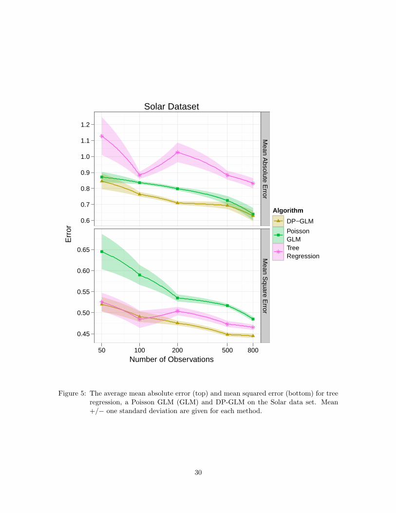
The competitors on this dataset are tree regression and a Poisson GLM. Frequentistestimation of the Poisson GLM produced unstable estimates as some of the covariates arecolinear. This problem was addressed by estimating the parameters in a Bayesian mannerwith Gaussian priors. Mean absolute (L1) error and mean squared (L2) error for 50, 100,200, 500, and 800 training data were computed using 10 random subset selections for eachamount of data. In DP-GLM, a Gaussian base measure was used for the GLM parametersand a Dirichlet for the covariates. Results are given in Figure 5.

Tree regression has a relatively low mean absolute error, while it has a high mean squarederror. The Poisson GLM has the opposite, relatively low mean squared error and relativelyhigh mean absolute error. Only the DP-GLM does well under both metrics.

Discussion. DP-GLM has flexibility that is not offered by most regression methods. Itdoes well on data sets with heteroscedastic errors because it fundamentally incorporatesthem; error parameters (σi,y) are included in the DP mixture. DP-GLM is comparativelyrobust with small amounts of data because in that case it tends to put all (or most) of theobservations into one cluster; this effectively produces a linear regression, but eliminatesoutliers by placing them into their own (low-weighted) clusters.

The comparison between DP-GLM regression and basic DP regression is illustrative.We compared basic DP regression only on the CCS data set because it has a large numberof covariates. Like kernel smoothing, basic DP regression struggles in high dimensionsbecause it cannot efficiently interpolate values between observations. The GLM componenteffectively eliminates this problem.

The diversity of the data sets demonstrates the adaptability of the DP-GLM. Onlytree regression was able to work on all of the data sets as well, and the DP-GLM has manydesirable properties that tree regression does not, such as a smooth mean function estimate.Moreover, the DP-GLM usually outperformed tree regression.

28

CCS Dataset

Number of Observations

Err

or

0.2

0.3

0.4

0.5

0.6

0.7

0.8

0.9

0.3

0.4

0.5

0.6

0.7

30 50 100 250 500

Mean A

bsolute Error

Mean S

quare Error

Algorithm

DP−GLM

OLS

TreeRegressionGaussianProcess

LocationScale DP

Figure 4: The average mean absolute error (top) and mean squared error (bottom) for ordi-nary least squares (OLS), tree regression, Gaussian processes, location/scale DPand the DP-GLM Poisson model on the CCS data set. The data were normalized.Mean +/− one standard deviation are given for each method.

29

Solar Dataset

Number of Observations

Err

or

0.6

0.7

0.8

0.9

1.0

1.1

1.2

0.45

0.50

0.55

0.60

0.65

50 100 200 500 800

Mean A

bsolute Error

Mean S

quare Error

Algorithm

DP−GLM

PoissonGLMTreeRegression

Figure 5: The average mean absolute error (top) and mean squared error (bottom) for treeregression, a Poisson GLM (GLM) and DP-GLM on the Solar data set. Mean+/− one standard deviation are given for each method.

30

6. Conclusions and Future Work

We have developed the DP-GLM, a flexible model for nonparametric Bayesian regression.We conditions for asymptotic unbiasedness and gave a specific case for when it is asymp-totically unbiased with conjugate priors. We then tested the DP-GLM on a variety ofdata sets to demonstrate its flexibility in the face of common statistical problems such asdata type (continuous, count, categorical, etc), heteroscedastic errors and moderately highdimensionality.

The DP-GLM offers a framework for a variety of predictive models. Our future workincludes using a shape-restricted function in place of the GLM to create a regression modelfor functions that are known to be concave in one dimension. Such regression problemsoften arise in a simulation-optimization setting where one dimension is resource amount,the others are state and the response is resource value. The methods provided in this papergive a way to construct and theoretically analyze many flexible yet complicated models withDirichlet process priors.

Appendix

A-1 Proofs for Section 4.3

Proof [Proof of Lemma 12.] G0 is a measure on the space Rd+1 ×Rd+1+ ×Rd. The induced

parameters are on the space R×Rd+1+ ×Rd. Suppose P ∼ DP (α,G0) and P is the random

measure on the induced parameters. Define G0 as above. Fix a finite partition of R ×Rd+1

+ × Rd, B1, . . . , Bk. For convenience of notation, break Bi into Bi,1 ×Bi,2 ×Bi,3 alongthe components of the product space. Define Bi,1 = β0:d : β0 + β1x1 + · · ·+ βdxd ∈ Bi,1.Then,(

P (B1), . . . , P (Bk))

=(P (B1,1 ×B1,2 ×B1,3), . . . , P (Bk,1 ×Bk,2 ×Bk,3)

)∼ Dir

(αG0(B1,1 ×B1,2 ×B1,3), . . . , αG0(Bk,1 ×Bk,2 ×Bk,3)

)= Dir

(G0(B1), . . . , G0(Bk)

).

This extends Remark 3 of Ghosal et al. (1999) to our multidimensional setting. It isused in the proof of Lemma 13.

Lemma A-1 Let f0(x, y) be a density on Rd × R. Suppose that there exists a closed setD ⊂ Rd × R such that there exists c > 0 where f0(x, y) > c for every (x, y) ∈ D and thex domain of D is a hypercube. Suppose that f0(x, y) = 0 if x is outside of D, and assumethat for y outside of D, f0(x, y) is increasing in y below D, and decreasing in y above D.Define for h = (h1, . . . , hd, hy),

f0,h(x, y) =∫

Rd+1

f0(µ1, . . . , µd, η)φhy(y − η)d∏i=1

φhi(x− µi)dµ1 . . . dµddη.

31

If ∫Rd+1

f0(x, y) log f0(x, y)dx1 . . . dxddy <∞,

then for every ε > 0 there exists h = (h1, . . . , hd, hy) > 0 such that,∫Rd+1

f0(x, y) logf0(x, y)f0,h(x, y)

dxdy < ε.

Proof For every x ∈ D, assume that the minimum width of the interval for which y ∈ Dis at least a1(x) and at most a2(x) for some functions 0 < a1(x) ≤ a2(x). If this is nottrue, we can simply change the x domain of D until it is true. Let a be the maximum valuefor y ∈ D and a be the minimum value. Let (x1, . . . , xd) be the upper left corner of the xhypercube, and (x1, . . . , xd) be the lower right. Now, choose h0 = (h0,y, h0,1, . . . , h0,d) suchthat N(0, h0,i) give probability 1/2 to the xi domain of D, and N(0, h0,y) gives probabilityb1 to (0, a1) and probability b2 to (0, a2), with 0 < b1 ≤ b2 < 1. Set h < h0. If (x, y) ∈ D,

f0,h(x, y) ≥∫Df0(µ1, . . . , µd, η)φhy(y − η)

d∏i=1

φhi(xi − µi)dµ1 . . . dµddη,

≥ c (Φ((a− y)/hy) + Φ((y − a)/hy))d∏i=1

(Φ((xi − xi)/hi) + Φ((xi − xi)/hi)) ,

≥ c b12d.

If y /∈ D and y > a2(x) given x, then

f0,h(x, y) ≥∫µ∈D

∫η>a2(x)

f0(µ1, . . . , µd, η)φhy(y − η)d∏i=1

φhi(xi − µi)dµ1 . . . dµddη,

≥ f0(x, y) (1/2 + Φ(a/hy)− 1)d∏i=1

(Φ((xi − xi)/hi) + Φ((xi − xi)/hi)) ,

≥ f0(x, y)b22d.

Using a similar argument when y < a1(x) for a given x, we have a function

g(x, y) =

log(2df0(x, y)/(b1c)), if (x, y) ∈ Dlog(2d/b2), if (x, y) /∈ D,

dominates log(f0(x, y)/f0,h(x, y)) for h < h0 and x ∈ D and is Pf0-integrable (outsideD for x, f0(x, y) is assumed to have 0 density). For all continuity points (x, y) of f0,f0(x, y)/f0,h(x, y) → 1 as h → 0; since

∫f0 log(f0/f0,h) ≥ 0, an application of Fatou’s

lemma shows that∫f0 log(f0/f0,h)→ 0 as h→ 0.

We can now prove Lemma 13.Proof [Proof of Lemma 13.] This proof strongly follows the proof of Lemma 3.2 in Tokdar(2006).

32

Fix x. Fix 0 < τ < 1 and ε > 0. By assumption, find A and y0 such that ΠP (A) > 1−τfor any P ∈ A, ∫

|y|>y0f0(x, y) log

f0(x, y)f(x, y)

dy < εf0(x)

4. (A-1)

Now consider the region where f0(x, y) is truncated to the interval [−y0, y0]. FromLemma A-1, there exist a h = (h1, . . . , hd, hy) > 0 and k1, k1, . . . , kd, kd, ky, ky such that

∫ y0

−y0f0(x, y) log

f0(x, y)∫ k1

k1

∫ kykyf0(µ1, . . . , µd, η)φhy(y − η)

∏di=1 φhi(xi − µi)dµ1 . . . dη

dy < εf0(x)

4,

(A-2)and ∣∣∣∣∣∣log

f0(x)∫ k1

k1. . .∫ kdkdf0(µ1, . . . , µd)

∏di=1 φhi(xi − µi)dµ1 . . . dµd

∣∣∣∣∣∣ < ε

8. (A-3)

Let P0 be a measure over the location and scale for all components on Rd+1×Rd+1+ , such

that dP0 = f0(x, y)×δh1×· · ·×δhy . Fix κ > 0 and find λ > 0 such that 1−λ/(κ2(1−λ)2) > τ .Choose a compact set K such that [k1, k1]×· · ·× [ky, ky]×h1×· · ·×hy ⊂ K, G0(K) >1− λ and P0(K) > 1− λ. Let B = P : |P (K)/P0(K)− 1| < κ. Since the prior on P is aDirichlet process, P (K) ∼ Beta(αG0(K), αG0(Kc)). By applying Markov’s inequality,

ΠP (B) ≥ 1− E(P (K)− P0(K))2

κ2P0(K)2≥ 1− λ

κ2(1− λ)2> τ.

Therefore, ΠP (A ∩ B) > 0.

Following Tokdar (2006) and Ghosal et al. (1999), we can find a set C such that ΠP (A∩B ∩ C) > 0 and P ∈ B ∩ C implies that for suitable κ,

∫ y0

−y0f0(x, y) log

∫K φσy(y − η)

∏di=1 φσi(xi − µi)dP0∫

K φσy(y − η)∏di=1 φσi(xi − µi)dP

dy <κ

1− κ+ 2κ < ε

f0(x)4

, (A-4)

and ∣∣∣∣∣log

∫Kx

∏di=1 φσi(xi − µi)dP0,x∫

Kx

∏di=1 φσi(xi − µi)dPx

∣∣∣∣∣ < κ

1− κ+ 2κ <

ε

8. (A-5)

33

Now let f = φd+1 ∗ P , where P ∈ A ∩ B ∩ C,∫f0(y|x) log

f0(y|x)f(y|x)

dy ≤ 1f0(x)

∫|y|>y0

f0(x, y) logf0(x, y)f(x, y)

dy

+

∣∣∣∣∣∣logf0(x)∫ k1

k1. . .∫ kdkdf0(µ1, . . . , µd)

∏di=1 φhi(xi − µi)dµ1 . . . dµd

∣∣∣∣∣∣+

∣∣∣∣∣log

∫Kx

∏di=1 φσi(xi − µi)dP0,x∫

Kx

∏di=1 φσi(xi − µi)dPx

∣∣∣∣∣+

1f0(x)

(∫ y0

−y0f0(x, y) log

∫K φσy(y − η)

∏di=1 φσi(xi − µi)dP0∫

K φσy(y − η)∏di=1 φσi(xi − µi)dP

dy

+∫ y0

−y0f0(x, y) log

f0(x, y)∫ k1

k1. . .∫ kykyf0(µ1, . . . , µd, η)φhy(y − η)

∏di=1 φhi(xi − µi)dµ1 . . . dη

dy

< ε,

by equations (A-1), (A-2), (A-3), (A-4) and (A-5).

Proof [Proof of Theorem 14.] To prove this Theorem, we need to show that such an f0

and G0 satisfy Lemma 13. This proof is very similar to the proof of Theorem 3.3 in Tokdar(2006). Let w(x) = exp(−xγ), x ≥ 0. Define a class of subsets of Rd+1×Rd+1

+ indexed onlyby y ∈ R (since x is fixed) as follows,

K(y)c =

(µ1, σ1)× · · · × (η, σy) ∈ Rd+1 × Rd+1+ : φσi(xi − µi) ≥ c,

φσy(y − η) ≥ (2π)−1/2w(|y|).

Let f = φd+1 ∗ P ,∫|y|>y0

f0(x, y) logf0(x, y)f(x, y)

dy

≤∫|y|>y0

f0(x, y) logf0(x, y)∫

K(y)cφσy(y − η)

∏di=1 φσi(xi − µi)dP

dy,

≤∫|y|>y0

f0(x, y) logf0(x, y)

(2π)−2/2w(|y|)cdP (K(y)c)dy,

≤∫|y|>y0

f0(x, y)

log f0(x, y) + |y|γ + log

(2π)1/2

cdP (K(y)c)

dy. (A-6)

We can show that equation (A-6) can be made arbitrarily small for suitably large y0 ifP (K(y)c) > a1 exp(−a2|y|γ) for all |y| > y0 for some fixed constants a1, a2 > 0. To showthis, we slightly modify Lemma 3.3 of Tokdar (2006).

34

Lemma A-2 (Modification of Lemma 3.3 of Tokdar (2006)) For any τ > 0 thereexists a y0 > 0, a c > 0 and a set A with Π(A) > 1 − τ such that P ∈ A ⇒ P (K(y)c) ≥(1/2)b1 exp(−2|y|γ/b2) for all |y| > y0.

The proof follows the lines of the original proof, but relies on the independence of the basemeasure G0 for the x and y dimensions.

A-2 Extension of Section 4.3 to Categorical Covariates

Assume that X is a set of categorical random variables taking values in the finite set D. Toextend Theorem 14 to include categorical covariates, we must define terms, redefine howthe random density is constructed and then modify assumptions. Let M(x|p) denote themultinomial probability mass function with one outcome and probability vector p evaluatedat x. Let P be the probability simplex for p.

For simplicity, we assume that there is only one covariate; extension to multiple covari-ates is straightforward. We construct the random density fP in the following manner,

fP (x, y) =∫P×R×R+

φσy(y − η)M(x|p)P (dp, dη, dσy).

We need the assumptions:

A1) f0(x) > 0 for every x ∈ D,

A2)∫D×R f0(x, y) log f0(x, y)dxdy <∞,

A3) for any fP with P ∈ A, ∫|y|>y0

f0(x, y) logf0(x, y)f(x, y)

dy < ε.

Now, we sketch how the inclusion of a categorical covariate affects Lemmas A-1, 13 andTheorem 14. We do not need to change Lemma A-2.

Categorical Covariates in Lemma A-1. We modify this Lemma in the following man-ner:

L1) Suppose that there exists a c > 0 and a y0 such that for every x ∈ D and |y| ≤ y0,f0(x) > c and f0(y|x) > c,

L2) Define

f0,h(x, y) =∫

Rf0(x, η)φh(y − η)dη.

The proof of the Lemma proceeds in the same manner as before.

35

Categorical Covariates in Lemma 13. First, modify Lemma 13 by replacing conditionsi), ii) and iv) with assumptions A1), A2) and A3), respectively. These assumptions areanalogous to those in the continuous setting.

Next, because Lemma A-2 is not completely analogous, we need to change equations(A-2) and (A-3). Using Lemma A-2, we can choose an h and k, k such that,∫ y0

−y0f0(x, y) log

f0(x, y)∫ kk f0(x, η)φh(y − η)dη

dy < εf0(x)

8. (A-7)

. Using the fact that for every δ > 0 we can choose a closed set E ⊂ P that contains anon-empty interior such that |f0(x)−

∫EM(x|p)dp| < δ, we can choose E such that,

∫ y0

−y0f0(x, y) log

∫ kk f0(x, η)φh(y − η)dη∫ k

k

∫E f0(η|x)φh(y − η)M(x|p)dηdp

dy < εf0(x)

8, (A-8)

and ∣∣∣∣logf0(x)∫

EM(x|p)dp

∣∣∣∣ < ε

8. (A-9)

Equations (A-7) and (A-8) take the place of equation (A-2), while equation (A-9) takes theplace of equation (A-3).

Let p0 be the multinomial parameters of f0(x) (which is multinomial because X iscategorical), and P0 be a measure over R×R+×P. Define dP0 = f(y|x)× δh× δp0 . Choosecompact K such that [k, k]× h× p0 ⊂ K. The rest of the proof follows.

Categorical Covariates in Theorem 14. Modify Theorem 14 by replacing assumptionsi) and ii) with A1) and A2), respectively. Now we simply need to change the way K(y)c isdefined,

K(y)c =p× (η, σy) ∈ P × R× R+ :M(x|p) ≥ c, φσy(y − η) ≥ (2π)−1/2w(|y|)

.

The rest of the proof follows.

Categorical Covariates with Conjugate Base Measure. The tail properties of G0,y

are the limiting factor in Theorem 14; for the covariate base measure, the only majorrequirement is that every open set that approximates f0(x) > c arbitrarily well has apositive measure. For every δ > 0, a conjugate base measure (Dirichlet) places positivemeasure on p : |f0(x)−M(x|p)| < δ when f0(x) > c.

A-3 Extension of Section 4.3 to Count Covariates

This subsection proceeds in a similar manner to the previous subsection. Assume that Xis a count random variable taking values in Z+. Let P(x|λ) denote the Poisson probabilitymass function with parameter λ evaluated at x.

For simplicity, we assume that there is only one covariate; extension to multiple covari-ates is straightforward. We construct the random density fP in the following manner,

fP (x, y) =∫

R+×R×R+

φσy(y − η)P(x|λ)P (dλ, dη, dσy).

36

We need the assumptions:

B1) f0(x) > 0 for every x ∈ D, where D is a bounded set,

B2)∫D×R f0(x, y) log f0(x, y)dxdy <∞,

B3) for any fP with P ∈ A, ∫|y|>y0

f0(x, y) logf0(x, y)f(x, y)

dy < ε.

Modify Lemma A-1 as before. We now explain how to modify Lemma 13 and Theorem 14.

Count Covariates in Lemma 13. Modify Lemma 13 by replacing conditions i), ii) andiv) with assumptions B1), B2) and B3), respectively.

Again, because Lemma A-2 is not completely analogous, we need to change equations(A-2) and (A-3). Using Lemma A-2, we can choose an h and k, k such that,∫ y0

−y0f0(x, y) log

f0(x, y)∫ kk f0(x, η)φh(y − η)dη

dy < εf0(x)

8. (A-10)

. Using the fact that for every δ > 0 we can choose `, ` such that |f0(x)−∫ `` P(x|λ)dλ| < δ,

∫ y0

−y0f0(x, y) log

∫ kk f0(x, η)φh(y − η)dη∫ k

k

∫ `` f0(η|x)φh(y − η)P(x|λ)dηdλ

dy < εf0(x)

8, (A-11)

and ∣∣∣∣∣∣logf0(x)∫ `

` P(x|λ)dλ

∣∣∣∣∣∣ < ε

8. (A-12)

Equations (A-10) and (A-11) take the place of equation (A-2), while equation (A-12) takesthe place of equation (A-3).

Let λ0 be the Poisson parameter of f0(x), were f0(x) modeled as a Poisson randomvariable, and P0 be a measure over R × R+ × R+. Define dP0 = f(y|x) × δh × δλ0 . Notethat the `, ` from above can be chosen such that ` < λ0 < `. Choose compact K such that[k, k]× h× λ0 ⊂ K. The rest of the proof follows.

Categorical Covariates in Theorem 14. Modify Theorem 14 by replacing assumptionsi) and ii) with B1) and B2), respectively. Now change the way K(y)c is defined,

K(y)c =λ× (η, σy) ∈ P × R× R+ : P(x|λ) ≥ c, φσy(y − η) ≥ (2π)−1/2w(|y|)

.

The rest of the proof follows.

Count Covariates with Conjugate Base Measure. The conjugate base measure is aGamma distribution. Like above, the conjugate distribution places positive measure on allweak sets around f0(x). Unlike above, our conclusions hold only for queries in a boundedregion (this is not a problem for categorical covariates).

37

References

M. Amewou-Atisso, S. Ghosal, J.K. Ghosh, and RV Ramamoorthi. Posterior consistencyfor semi-parametric regression problems. Bernoulli, pages 291–312, 2003.

C.E. Antoniak. Mixtures of Dirichlet processes with applications to Bayesian nonparametricproblems. The Annals of Statistics, 2(6):1152–1174, 1974.

A. Barron, M.J. Schervish, and L. Wasserman. The consistency of posterior distributionsin nonparametric problems. The Annals of Statistics, 27(2):536–561, 1999.

CL Bennett, M. Halpern, G. Hinshaw, N. Jarosik, A. Kogut, M. Limon, SS Meyer,L. Page, DN Spergel, GS Tucker, et al. First-Year Wilkinson Microwave AnisotropyProbe (WMAP) 1 Observations: Preliminary Maps and Basic Results. The AstrophysicalJournal Supplement Series, 148(1):1–27, 2003.

P. Billingsley. Probability and measure. Wiley India Pvt. Ltd., 2008.

D. Blackwell and J.B. MacQueen. Ferguson distributions via Polya urn schemes. The AnnalsStatistics, 1(2):353–355, 1973.

D.M. Blei and M.I. Jordan. Variational inference for Dirichlet process mixtures. BayesianAnalysis, 1(1):121–144, 2005.

G. Bradshaw. UCI machine learning repository, 1989. URLhttp://www.ics.uci.edu/∼mlearn/MLRepository.html.

L. Brieman, J.H. Friedman, R.A. Olshen, and C.J. Stone. Classification and RegressionTrees. Wadsworth, 1984.

S.P. Brooks and A. Gelman. General methods for monitoring convergence of iterativesimulations. Journal of Computational and Graphical Statistics, pages 434–455, 1998.

M. De Iorio, P. Muller, G.L. Rosner, and S.N. MacEachern. An ANOVA model for depen-dent random measures. Journal of the American Statistical Association, 99(465):205–215,2004.

P. Diaconis and D. Freedman. On the consistency of Bayes estimates. The Annals ofStatistics, 14(1):1–26, 1986.

J.A. Duan, M. Guindani, and A.E. Gelfand. Generalized spatial Dirichlet process models.Biometrika, 94(4):809–825, 2007.

D.B. Dunson, N. Pillai, and J.H. Park. Bayesian density regression. Journal of the RoyalStatistical Society: Series B (Statistical Methodology), 69(2):163–183, 2007.

M.D. Escobar. Estimating normal means with a Dirichlet process prior. Journal of theAmerican Statistical Association, pages 268–277, 1994.

M.D. Escobar and M. West. Bayesian Density Estimation and Inference Using Mixtures.Journal of the American Statistical Association, 90(430):577–588, 1995.

38

J. Fan and I. Gijbels. Data-driven bandwidth selection in local polynomial fitting: variablebandwidth and spatial adaptation. Journal of the Royal Statistical Society. Series B(Methodological), pages 371–394, 1995.

J. Fan and I. Gijbels. Local Polynomial Modelling and Its Applications. Chapman &Hall/CRC, 1996.

P. Fearnhead. Particle filters for mixture models with an unknown number of components.Statistics and Computing, 14(1):11–21, 2004.

T.S. Ferguson. A Bayesian analysis of some nonparametric problems. The Annals of Statis-tics, 1(2):209–230, 1973.

J.H. Friedman. Multivariate adaptive regression splines. The Annals of Statistics, 19(1):1–141, 1991.

A.E. Gelfand, A. Kottas, and S.N. MacEachern. Bayesian nonparametric spatial modelingwith Dirichlet process mixing. Journal of the American Statistical Association, 100(471):1021–1035, 2005.

A. Gelman, J.B. Carlin, and H.S. Stern. Bayesian data analysis. CRC press, 2004.

S. Ghosal and A. van der Vaart. Posterior convergence rates of Dirichlet mixtures at smoothdensities. Annals of statistics, 35(2):697, 2007.

S. Ghosal, JK Ghosh, and RV Ramamoorthi. Posterior consistency of Dirichlet mixtures indensity estimation. The Annals of Statistics, 27(1):143–158, 1999.

S. Ghosal, J.K. Ghosh, and A.W. van der Vaart. Convergence rates of posterior distribu-tions. Annals of Statistics, pages 500–531, 2000.

JK Ghosh and RV Ramamoorthi. Bayesian Nonparametrics. Springer, 2003.

JE Griffin and M.F.J. Steel. Order-based dependent Dirichlet processes. Journal of theAmerican Statistical Association, 101(473):179–194, 2006.

JE Griffin and MFJ Steel. Bayesian nonparametric modelling with the Dirichlet processregression smoother. Technical report, Technical Report, Institute of Mathematics, Statis-tics and Actuarial Science, University of Kent, 2007.

T. Hastie, R. Tibshirani, and J. Friedman. The Elements of Statistical Learning: DataMining, Inference, and Prediction, Second Edition. Springer, 2009.

J.G. Ibrahim and K.P. Kleinman. Semiparametric Bayesian methods for random effectsmodels. Practical Nonparametric and Semiparametric Bayesian Statistics, pages 89–114,1998.

J. Lafferty and L. Wasserman. Rodeo: Sparse, greedy nonparametric regression. The Annalsof Statistics, 36(1):28–63, 2008.

39

N. Lawrence, M. Seeger, and R. Herbrich. Fast sparse Gaussian process methods: Theinformative vector machine. Advances in neural information processing systems, pages625–632, 2003.

S.N. MacEachern. Estimating normal means with a conjugate style Dirichlet process prior.Communications in Statistics-Simulation and Computation, 23(3):727–741, 1994.

S.N. MacEachern and P. Muller. Estimating mixture of Dirichlet process models. Journalof Computational and Graphical Statistics, 7(2):223–238, 1998.

P. McCullagh and J.A. Nelder. Generalized Linear Models. Chapman & Hall/CRC, 1989.

S. Mukhopadhyay and A.E. Gelfand. Dirichlet Process Mixed Generalized Linear Models.Journal of the American Statistical Association, 92(438):633–639, 1997.

P. Muller, A. Erkanli, and M. West. Bayesian curve fitting using multivariate normalmixtures. Biometrika, 83(1):67–79, 1996.

R.M. Neal. Markov chain sampling methods for Dirichlet process mixture models. Journalof Computational and Graphical Statistics, 9(2):249–265, 2000.

T. Nicoleris and S.G. Walker. On a posterior predictive density sample size criterion.Scandinavian Journal of Statistics, 33(2):209–218, 2006.

J. Pitman. Some developments of the Blackwell-MacQueen urn scheme. Lecture Notes-Monograph Series, pages 245–267, 1996.

J. Quinonero-Candela and C.E. Rasmussen. A unifying view of sparse approximate Gaussianprocess regression. The Journal of Machine Learning Research, 6:1939–1959, 2005.

C.E. Rasmussen and C.K.I. Williams. Gaussian processes for machine learning. Springer,2006.

A. Rodriguez, D.B. Dunson, and A.E. Gelfand. Bayesian nonparametric functional dataanalysis through density estimation. Biometrika, 96(1):149–162, 2009.

D. Ruppert, SJ Sheather, and MP Wand. An effective bandwidth selector for local leastsquares regression. Journal of the American Statistical Association, pages 1257–1270,1995.

L. Schwartz. On Bayes procedures. Z. Wahrsch. Verw. Gebiete, 4(1):10–26, 1965.

J. Sethuraman. A constructive definition of the Dirichlet process. Statist. Sinica, 4:639–650,1994.

B. Shahbaba and R.M. Neal. Nonlinear Models Using Dirichlet Process Mixtures. Journalof Machine Learning Research, 10:1829–1850, 2009.

X. Shen. Asymptotic normality of semiparametric and nonparametric posterior distribu-tions. Journal of the American Statistical Association, 97(457):222–235, 2002.

40

X. Shen and L. Wasserman. Rates of convergence of posterior distributions. Annals ofStatistics, pages 687–714, 2001.

A.J. Smola and B. Scholkopf. A tutorial on support vector regression. Statistics andComputing, 14(3):199–222, 2004.

E. Snelson and Z. Ghahramani. Sparse Gaussian processes using pseudo-inputs. Advancesin Neural Information Processing Systems, 18:1257, 2006.

S. Tokdar. Posterior consistency of Dirichlet location-scale mixture of normals in densityestimation and regression. Sankhya: The Indian Journal of Statistics, 67:90–110, 2006.

S. Walker. New approaches to Bayesian consistency. The Annals of Statistics, 32(5):2028–2043, 2004.

S.G. Walker, A. Lijoi, and I. Prunster. On rates of convergence for posterior distributionsin infinite-dimensional models. Annals of Statistics, 35(2):738, 2007.

M. West, P. Muller, and M.D. Escobar. Hierarchical priors and mixture models, withapplication in regression and density estimation. Aspects of uncertainty: A Tribute toDV Lindley, pages 363–386, 1994.

I.C. Yeh. Modeling of strength of high-performance concrete using artificial neural networks.Cement and Concrete research, 28(12):1797–1808, 1998.

41