nonlinear models using dirichlet process mixtures - journal of

Journal of Machine Learning Research 10 (2009) 1829-1850 Submitted 5/08; Revised 11/08; Published 8/09

Nonlinear Models Using Dirichlet Process Mixtures

Babak Shahbaba [email protected]

Department of StatisticsUniversity of California at IrvineIrvine, CA, USA

Radford Neal [email protected]

Departments of Statistics and Computer ScienceUniversity of TorontoToronto, ON, Canada

Editor: Zoubin Ghahramani

AbstractWe introduce a new nonlinear model for classification, in which we model the joint distribution ofresponse variable,y, and covariates,x, non-parametrically using Dirichlet process mixtures. Wekeep the relationship betweeny andx linear within each component of the mixture. The overallrelationship becomes nonlinear if the mixture contains more than one component, with differentregression coefficients. We use simulated data to compare the performance of this new approachto alternative methods such as multinomial logit (MNL) models, decision trees, and support vectormachines. We also evaluate our approach on two classification problems: identifying the foldingclass of protein sequences and detecting Parkinson’s disease. Our model can sometimes improvepredictive accuracy. Moreover, by grouping observations into sub-populations (i.e., mixture com-ponents), our model can sometimes provide insight into hidden structure in the data.Keywords: mixture models, Dirichlet process, classification

1. Introduction

In regression and classification models, estimation of parameters and interpretation of results areeasier if we assume that distributions have simple forms (e.g., normal) and that the relationshipbetween a response variable and covariates is linear. However, the performance of such a modeldepends on the appropriateness of these assumptions. Poor performance may result from assum-ing wrong distributions, or regarding relationships as linear when they arenot. In this paper, weintroduce a new model based on a Dirichlet process mixture of simple distributions, which is moreflexible in capturing nonlinear relationships.

A Dirichlet process,D(G0,γ), with baseline distributionG0 and scale parameterγ, is a dis-tribution over distributions. Ferguson (1973) introduced the Dirichlet process as a class of priordistributions for which the support is large, and the posterior distribution is manageable analyti-cally. Using the Polya urn scheme, Blackwell and MacQueen (1973) showed that the distributionssampled from a Dirichlet process are discrete almost surely.

The idea of using a Dirichlet process as the prior for the mixing proportionsof a simple dis-tribution (e.g., Gaussian) was first introduced by Antoniak (1974). In thispaper, we will describethe Dirichlet process mixture model as a limit of a finite mixture model (see Neal, 2000, for furtherdescription). Suppose exchangeable random valuesy1, ...,yn are drawn independently from some

c©2009 Babak Shahbaba and Radford Neal.

SHAHBABA AND NEAL

unknown distribution. We can model the distribution ofy as a mixture of simple distributions, withprobability or density function

P(y) =C

∑c=1

pcF(y,φc).

Here,pc are the mixing proportions, andF(y,φ) is the probability or density fory under a distribu-tion, F(φ), in some simple class with parametersφ—for example, a normal in whichφ = (µ,σ). Wefirst assume that the number of mixing components,C, is finite. In this case, a common prior forpc

is a symmetric Dirichlet distribution, with density function

P(p1, ..., pC) =Γ(γ)

Γ(γ/C)C

C

∏c=1

p(γ/C)−1c ,

wherepc ≥ 0 and∑ pc = 1. The parametersφc are independent under the prior, with distributionG0. We can use mixture identifiers,ci , and represent this model as follows:

yi |ci ,φ ∼ F(φci ),

ci |p1, ..., pC ∼ Discrete(p1, ..., pC),

p1, ..., pC ∼ Dirichlet(γ/C, ....,γ/C),

φc ∼ G0.

(1)

By integrating over the Dirichlet prior, we can eliminate the mixing proportions,pc, and obtain thefollowing conditional distribution forci :

P(ci = c|c1, ...,ci−1) =nic + γ/Ci−1+ γ

. (2)

Here,nic represents the number of data points previously (i.e., before theith) assigned to componentc. As we can see, the above probability becomes higher asnic increases.

WhenC goes to infinity, the conditional probabilities (2) reach the following limits:

P(ci = c|c1, ...,ci−1) →nic

i−1+ γ,

P(ci 6= c j for all j < i|c1, ...,ci−1) →γ

i−1+ γ.

As a result, the conditional probability forθi , whereθi = φci , becomes

θi |θ1, ...,θi−1 ∼1

i−1+ γ ∑j<i

δθ j +γ

i−1+ γG0, (3)

whereδθ is a point mass distribution atθ. Since the observations are assumed to be exchangeable,we can regard any observation,i, as the last observation and write the conditional probability ofθi

given the otherθ j for j 6= i (written θ−i) as follows:

θi |θ−i ∼1

n−1+ γ ∑j 6=i

δθ j +γ

n−1+ γG0. (4)

1830

NONLINEAR MODELS USING DIRICHLET PROCESSM IXTURES

The above conditional probabilities are equivalent to the conditional probabilities forθi accordingto the Dirichlet process mixture model (as presented by Blackwell and MacQueen, 1973, using thePolya urn scheme), which has the following form:

yi |θi ∼ F(θi),

θi |G ∼ G, (5)

G ∼ D(G0,γ).

That is, If we letθi = φci , the limit of model (1) asC → ∞ becomes equivalent to the Dirichletprocess mixture model (Ferguson, 1983; Neal, 2000). In model (5),G is the distribution overθ’s,and has a Dirichlet process prior,D. Phrased this way, each data point,i, has its own parameters,θi , drawn independently from a distribution that is drawn from a Dirichlet process prior. But sincedistributions drawn from a Dirichlet process are discrete (almost surely)as shown by Blackwell andMacQueen (1973), theθi for different data points may be the same.

The parameters of the Dirichlet process prior areG0, a distribution from whichθ’s are sampled,andγ, a positive scale parameter that controls the number of components of the mixture that willbe represented in the sample, such that a largerγ results in a larger number of components. Toillustrate the effect ofγ on the number of mixture components in a sample of size 200, we generatedsamples from four different Dirichlet process priors withγ = 0.1,1,5,10, and the same baselinedistributionG0 = N2(0,10I2) (whereI2 is a 2×2 identity matrix). For a given value ofγ, we firstsampleθi , wherei = 1, ...,200, according to the conditional probabilities (3), and then we sampleyi |θi ∼ N2(θi ,0.2I2). The data generated according to these priors are shown in Figure 1. Aswe cansee, the (prior) expected number of components in a finite sample increasesasγ becomes larger.

With a Dirichlet process prior, we can we find conditional distributions of theposterior distribu-tion of model parameters by combining the conditional prior probability of (4) with the likelihoodF(yi ,θi), obtaining

θi |θ−i ,yi ∼ ∑j 6=i

qi j δθ j + r iHi , (6)

whereHi is the posterior distribution ofθ based on the priorG0 and the single data pointyi , and thevalues of theqi j andr i are defined as follows:

qi j = bF(yi ,θ j),

r i = bγZ

F(yi ,θ)dG0(θ).

Here,b is such thatr i +∑ j 6=i qi j = 1. These conditional posterior distributions are what are neededwhen sampling the posterior using MCMC methods, as discussed further in Section 2.

Bush and MacEachern (1996), Escobar and West (1995), MacEachern and Muller (1998), andNeal (2000) have used Dirichlet process mixture models for density estimation. Muller et al. (1996)used this method for curve fitting. They model the joint distribution of data pairs(xi ,yi) as a Dirich-let process mixture of multivariate normals. The conditional distribution,P(y|x), and the expectedvalue,E(y|x), are estimated based on this distribution for a grid ofx’s (with interpolation) to obtaina nonparametric curve. The application of this approach (as presented by Muller et al., 1996) isrestricted to continuous variables. Moreover, this model is feasible only for problems with a smallnumber of covariates,p. For data with moderate to large dimensionality, estimation of the joint

1831

SHAHBABA AND NEAL

−10 −5 0 5 10−10

−5

0

5

10γ =0.1

X1

X2

−10 −5 0 5 10−10

−5

0

5

10γ =1

X1

X2

−10 −5 0 5 10−10

−5

0

5

10γ =5

X1

X2

−10 −5 0 5 10−10

−5

0

5

10γ =10

X1

X2

Figure 1: Data sets of sizen = 200 generated according to four different Dirichlet process mix-ture priors, each with the same baseline distribution,G0 = N2(0,10I2), but different scaleparameters,γ. As γ increases, the expected number of components present in the sam-ple becomes larger. (Note that, as can be seen above, whenγ is large, many of thesecomponents have substantial overlap.)

distribution is very difficult both statistically and computationally. This is mostly due tothe diffi-culties that arise when simulating from the posterior distribution of large full covariance matrices.In this approach, if a mixture model hasC components, the set of full covariance matrices haveCp(p+ 1)/2 parameters. For largep, the computational burden of estimating these parametersmight be overwhelming. Estimating full covariance matrices can also cause statistical difficultiessince we need to assure that covariance matrices are positive semidefinite.Conjugate priors basedthe inverse Wishart distribution satisfy this requirement, but they lack flexibility(Daniels and Kass,1999). Flat priors may not be suitable either, since they can lead to improper posterior distributions,and they can be unintentionally informative (Daniels and Kass, 1999). A common approach to ad-dress these issues is to use decomposition methods in specifying priors for full covariance matrices(see for example, Daniels and Kass, 1999; Cai and Dunson, 2006). Although this approach hasdemonstrated some computational advantages over direct estimation of full covariance matrices, itis not yet feasible for high-dimensional variables. For example, Cai andDunson (2006) recommendtheir approach only for problems with less than 20 covariates.

1832


We introduce a new nonlinear Bayesian model, which also nonparametrically estimatesP(x,y),the joint distribution of the response variabley and covariatesx, using Dirichlet process mixtures.Within each component, we assume the covariates are independent, and model the dependencebetweeny andx using a linear model. Therefore, unlike the method of Muller et al. (1996), ourapproach can be used for modeling data with a large number of covariates,since the covariancematrix for one mixture component is highly restricted. Using the Dirichlet process as the prior, ourmethod has a built-in mechanism to avoid overfitting since the complexity of the nonlinear modelis controlled. Moreover, this method can be used for categorical as well as continuous responsevariables by using a generalized linear model instead of the linear model.

The idea of building a nonlinear model based on an ensemble of simple linear models has beenexplored extensively in the field of machine learning. Jacobs et al. (1991) introduced a supervisedlearning procedure for models that are comprised of several local models (experts) each handling asubset of data. A gating network decides which expert should be used for a given data point. Forinferring the parameters of such models, Waterhouse et al. (1996) provided a Bayesian framework toavoid over-fitting and noise level under-estimation problems associated with traditional maximumlikelihood inference. Rasmussen and Ghahramani (2002) generalized mixture of experts models byusing infinitely many nonlinear experts. In their approach, each expert isassumed to be a Gaussianprocess regression model, and the gating network is based on an input-dependent adaptation ofDirichlet process. Meeds and Osindero (2006) followed the same idea, but instead of assuming thatthe covariates are fixed, they proposed a joint mixture of experts model over covariates and responsevariable.

Our focus here is on classification models with a multi-category response, in which we haveobserved data forn cases, (x1,y1),...,(xn,yn). Here, the classyi hasJ possible values, and the covari-atesxi can in general be a vector ofp covariates. We wish to classify future cases in which only thecovariates are observed. For binary (J = 2) classification problems, a simple logistic model can beused, with class probabilities defined as follows (with the case subscript dropped fromx andy):

P(y = 1|x,α,β) =exp(α+xTβ)

1+exp(α+xTβ).

When there are three or more classes, we can use a generalization knownas the multinomial logit(MNL) model (called “softmax” in the machine learning literature):

P(y = j|x,α,β) =exp(α j +xTβ j)

∑Jj ′=1exp(α j ′ +xTβ j ′)

.

MNL models arediscriminative, since they model the conditional distributionP(y|x), but notthe distribution of covariates,P(x). In contrast, our dpMNL model isgenerative, since it estimatesthe joint distribution of response and covariates,P(x,y). The joint distribution can be decomposeinto the product of the marginal distributionP(x) and the conditional distributionP(y|x); that is,P(x,y) = P(x)P(y|x).

Generative models have several advantages over discriminative models (see for example, Ulusoyand Bishop, 2005). They provide a natural framework for handling missing data or partially labeleddata. They can also augment small quantities of expensive labeled data with large quantities ofcheap unlabeled data. This is especially useful in applications such as document labeling and imageanalysis, where it may provide better predictions for new feature patternsnot present in the data at

1833

SHAHBABA AND NEAL

−4 −3 −2 −1 0 1 2 3 4−3

−2

−1

0

1

2

3

x1

x 2

Figure 2: An illustration of our model for a binary (black and white) classification problem withtwo covariates. Here, the mixture has two components, which are shown with circlesand squares. In each component, an MNL model separates the two classes into “black”or “white” with a linear decision boundary. The overall decision boundary, which is asmooth function, is not shown in this figure.

the time of training. For example, the Latent Dirichlet Allocation (LDA) model proposed by Bleiet al. (2003) is a well-defined generative model that performs well in classifying documents withpreviously unknown patterns.

While generative models are quite successful in many problems, they can becomputationally in-tensive. Moreover, finding a good (but not perfect) estimate for the joint distribution of all variables(i.e., x andy) does not in general guarantee a good estimate of decision boundaries.By contrast,discriminative models are often computationally fast and are preferred when the covariates are infact non-random (e.g., they are fixed by an experimental design).

Using a generative model in our proposed method provides an additional benefit. Modeling thedistribution of covariates jointly withy allows us to implicitly model the dependency of covariateson each other through clustering (i.e., assigning data points to different components), which couldprovide insight into hidden structure in the data. To illustrate this concept, consider Figure 2 wherethe objective is to classify cases into black or white. To improve predictive accuracy, our modelhas divided the data into two components, shown as squares and circles. These components aredistinguished primarily by the value of the second covariate,x2, which is usually positive for squaresand negative for circles. For cases in the squares group, the response variable strongly depends onbothx1 andx2 (the linear separator is almost diagonal), whereas, for cases in the circles group, themodel mainly depends onx1 alone (the linear model is almost vertical). Therefore, by grouping thedata into sub-populations (e.g., circles and squares in this example), our model not only improvesclassification accuracy, but also discovers hidden structure in the data (i.e., by clustering covariateobservations). This concept is briefly discussed in Section 5, where weuse our model to predictParkinson’s disease. A more detailed discussion on using our method to detect hidden structure in

1834


data is provided elsewhere (Shahbaba, 2009), where a Dirichlet process mixture of autoregressivemodels us used to analyze time-series processes that are subject to regime changes, with no specificeconomic theory about the structure of the model.

The next section describes our methodology. In Section 3, we illustrate ourapproach and evalu-ate its performance on simulated data. In Section 4, we present the results ofapplying our model toan actual classification problem, which attempts to identify the folding class of a protein sequencebased on the composition of its amino acids. Section 5 discusses another realclassification prob-lem, where the objective is to detect Parkinson’s disease. This example is provided to show howour method can be used not only for improving prediction accuracy, but also for identifying hiddenstructure in the data. Finally, Section 6 is devoted to discussion and future directions.

2. Methodology

We now describe our classification model, which we call dpMNL, in detail. We assume that for eachcase we observe a vector of continuous covariates,x, of dimensionp. The response variable,y, iscategorical, withJ classes. To model the relationship betweeny andx, we non-parametrically modelthe joint distribution ofy andx, in the formP(x,y) = P(x)P(y|x), using a Dirichlet process mixture.Within each component of the mixture, the relationship betweeny andx (i.e., P(y|x)) is expressedusing a linear function. The overall relationship becomes nonlinear if the mixture contains morethan one component. This way, while we relax the assumption of linearity, the flexibility of therelationship is controlled.

Each component in the mixture model has parametersθ = (µ,σ2,α,β). The distribution ofx within a component is multivariate normal, with mean vectorµ and diagonal covariance, withthe vectorσ2 on the diagonal. The distribution ofy given x within a component is given by amultinomial logit (MNL) model—for j = 1, . . . ,J,

P(y = j|x,α,β) =exp(α j +xTβ j)

∑Jj ′=1exp(α j ′ +xTβ j ′)

.

The parameterα j is scalar, andβ j is a vector of lengthp. Note that givenx, the distribution ofy doesnot depend onµ andσ. This representation of the MNL model is redundant, since one of theβ j ’s(where j = 1, ...,J) can be set to zero without changing the set of relationships expressiblewith themodel, but removing this redundancy would make it difficult to specify a priorthat treats all classessymmetrically. In this parameterization, what matters is the difference between the parameters ofdifferent classes.

In addition to the mixture view, which follows Equation (1) withC→ ∞, one can also view eachobservation,i, as having its own parameter,θi , drawn independently from a distribution drawn froma Dirichlet process, as in Equation (5):

θi |G ∼ G, for i = 1, . . . ,n,

G ∼ D(G0,γ).

SinceG will be discrete, many groups of observations will have identicalθi , corresponding tocomponents in the mixture view.

Although the covariates in each component are assumed to be independentwith normal priors,this independence of covariates exists only locally (within a component). Their global (over all

1835

SHAHBABA AND NEAL

components) dependency is modeled by assigning data to different components (i.e., clustering).The relationship betweeny andx within a component is captured using an MNL model. Therefore,the relationship is linear locally, but nonlinear globally.

We could assume thaty andx are independent within components, and capture the dependencebetween the response and the covariates by clustering too. However, thismay lead to poor per-formance (e.g., when predicting the response for new observations) if the dependence ofy on x isdifficult to capture using clustering alone. Alternatively, we could also assume that the covariatesare dependent within a component. For continuous response variables,this becomes equivalent tothe model proposed by Muller et al. (1996). If the covariates are in fact dependent, using full co-variance matrices (as suggested by Muller et al., 1996) could result in a more parsimonious modelsince the number of mixture component would be smaller. However, as we discussed above, thisapproach may be practically infeasible for problems with a moderate to large number of covariates.We believe that our method is an appropriate compromise between these two alternatives.

We defineG0, which is a distribution overθ = (µ,σ2,α,β), as follows:

µl |µ0,σ0 ∼ N(µ0,σ20),

log(σ2l )|Mσ,Vσ ∼ N(Mσ,V2

σ ),

α j |τ ∼ N(0,τ2),

β jl |ν ∼ N(0,ν2).

The parameters ofG0 may in turn depend on higher level hyperparameters. For example, we canregard the variances of coefficients as hyperparameters with the following priors:

log(τ2)|Mτ,Vτ ∼ N(Mτ,V2τ ),

log(ν2)|Mν,Vν ∼ N(Mν,V2ν ).

We use MCMC algorithms for posterior sampling. We could use Gibbs sampling ifG0 is theconjugate prior for the likelihood given byF . That is, we would repeatedly draw samples fromθi |θ−i ,yi (wherei = 1, ...,n) using the conditional distribution (6). Neal (2000) presented severalalgorithms for sampling from the posterior distribution of Dirichlet process mixtures when non-conjugate priors are used. Throughout this paper, we use Gibbs sampling with auxiliary parameters(Neal’s algorithm 8).

This algorithm uses a Markov chain whose state consists ofc1, ...,cn andφ = (φc : c∈{c1, ...,cn}),so thatθi = φci . In order to allow creation of new clusters, the algorithm temporarily supplementstheφc parameters of existing clusters withm (or m−1) additional parameter values drawn from theprior, wherem a postive integer that can be adjusted to give good performance. Each iteration ofthe Markov chain simulation operates as follows:

• For i = 1, ...,n: Let k− be the number of distinctc j for j 6= i and leth = k− +m. Label thesec j with values in{1, ...,k−}. If ci = c j for somej 6= i, draw values independently fromG0 forthoseφc for which k− < c≤ h. If ci 6= c j for all j 6= i, let ci have the labelk− +1, and drawvalues independently fromG0 for thoseφc wherek− + 1 < c ≤ h. Draw a new value forci

from {1, ...,h} using the following probabilities:

P(ci = c|c−i ,yi ,φ1, ...,φh) =

bn−i,c

n−1+ γF(yi ,φc) for 1≤ c≤ k−,

bγ/m

n−1+ γF(yi ,φc) for k− < c≤ h,

1836


wheren−i,c is the number ofc j for j 6= i that are equal toc, andb is the appropriate normalizingconstant. Change the state to contain only thoseφc that are now associated with at least toone observation.

• For all c ∈ {c1, ...,cn} draw a new value from the distributionφc | {yi such thatci = c}, orperform some update that leaves this distribution invariant.

Throughout this paper, we setm= 5. This algorithm resembles one proposed by MacEachern andMuller (1998), with the difference that the auxiliary parameters exist only temporarily, which avoidsan inefficiency in MacEachern and Muller’s algorithm.

Samples simulated from the posterior distribution are used to estimate posterior predictive prob-abilities. For a new case with covariatesx′, the posterior predictive probability of the responsevariable,y′, is estimated as follows:

P(y′ = j|x′) =P(y′ = j,x′)

P(x′),

where

P(y′ = j,x′) =1S

S

∑s=1

P(y′ = j,x′|G0,θ(s)),

P(x′) =1S

S

∑s=1

P(x′|G0,θ(s)).

Here, S is the number of post-convergence samples from MCMC, andθ(s) represents the set ofparameters obtained at iterations. Alternatively, we could predict new cases usingP(y′ = j,x′) =1S∑S

s=1P(y′ = j|x′,G0,θ(s)). While this would be computationally faster, the above approach allowsus to learn from the covariates of test cases when predicting their response values. Note also thatthe above predictive probabilities include the possibility that the test case is from a new cluster.

We use these posterior predictive probabilities to make predictions for test cases, by assigningeach test case to the class with the highest posterior predictive probability.This is the optimal strat-egy for a simple 0/1 loss function. In general, we could use more problem-specific loss functionsand modify our prediction strategy accordingly.

Implementations for all our models were coded in MATLAB, and are available online athttp://www.ics.uci.edu/ ˜ babaks/codes .

3. Results for Simulated Data

In this section, we illustrate our dpMNL model using synthetic data, and compare it with othermodels as follows:

• A simple MNL model, fitted by maximum likelihood or Bayesian methods.

• A Bayesian MNL model with quadratic terms (i.e.,xl xk, wherel = 1, ..., p andk = 1, ..., p),referred to as qMNL.

• A decision tree model (Breiman et al., 1993) that uses 10-fold cross-validation for pruning,as implemented by the MATLAB “treefit”, “treetest” (for cross-validation) and “treeprune”functions.

1837

SHAHBABA AND NEAL

• Support Vector Machines (SVMs) (Vapnik, 1995), implemented with the MATLAB “svm-train” and “svmclassify” functions from the Bioinformatics toolbox. Both a linear SVM(LSVM) and a nonlinear SVM with radial basis function kernel (RBF-SVM) were tried.

When the number of classes in a classification problem was bigger than two, LSVM and RBF-SVMused the all-vs-all scheme as suggested by Allwein et al. (2000), Furnkranz (2002), and Hsu andLin (2002). In this scheme,

(J2

)

binary classifiers are trained where each classifier separates a pairof classes. The predicted class for each test case is decided by using amajority voting schemewhere the class with the highest number of votes among all binary classes wins. For RBF-SVM,the scaling parameter,λ, in the RBF kernel,k(x,x′) = exp(−||x−x′||/2λ), was optimized based ona validation set comprised of 20% of training samples.

The models are compared with respect to their accuracy rate and theF1 measure. Accuracy rateis defined as the percentage of the times the correct class is predicted.F1 is a common measurementin machine learning defined as:

F1 =1J

J

∑j=1

2A j

2A j +B j +Cj,

whereA j is the number of cases which are correctly assigned to classj, B j is the number casesincorrectly assigned to classj, andCj is the number of cases which belong to the classj but areassigned to other classes.

We do two tests. In the first test, we generate data according to the dpMNL model. Our objectiveis to evaluate the performance of our model when the distribution of data is comprised of multiplecomponents. In the second test, we generate data using a smooth nonlinear function. Our goal is toevaluate the robustness of our model when data actually come from a different model.

3.1 Simulation 1

The first test was on a synthetic four-way classification problem with five covariates. Data aregenerated according to our dpMNL model, except the number of components was fixed at two. Twohyperparameters definingG0 were given the following priors:

log(τ2) ∼ N(0,0.12),

log(ν2) ∼ N(0,22).

The prior for component parametersθ = (µ,σ2,α,β) defined by thisG0 was

µl ∼ N(0,1),

log(σ2l ) ∼ N(0,22),

α j |τ ∼ N(0,τ2),

β jl |ν ∼ N(0,ν2),

wherel = 1, ...,5 and j = 1, ...,4. We randomly draw parametersθ1 andθ2 for two components asdescribed from this prior. For each component, we then generate 5000 data points by first drawingxil ∼ N(µl ,σl ) and then samplingy using the following MNL model:

P(y = j|x,α,β) =exp(α j +xβ j)

∑Jj ′=1exp(α j ′ +xβ j ′)

.

1838


Model Accuracy (%) F1 (%)

Baseline 45.57 (1.47) 15.48 (1.77)MNL (Maximum Likelihood) 77.30 (1.23) 66.65 (1.41)MNL 78.39 (1.32) 66.52 (1.72)qMNL 83.60 (0.99) 74.16 (1.30)Tree (Cross Validation) 70.87 (1.40) 55.82 (1.69)LSVM 78.61 (1.17) 67.03 (1.51)RBF-SVM 79.09 (0.99) 63.65 (1.44)dpMNL 89.21 (0.65) 81.00 (1.23)

Table 1: Simulation 1: the average performance of models based on 50 simulated data sets. TheBaseline model assigns test cases to the class with the highest frequency inthe trainingset. Standard errors of estimates (based on 50 repetitions) are providedin parentheses.

The overall sample size is 10000. We randomly split the data into a training set, with 100 datapoints, and a test set, with 9900 data points. We use the training set to fit the models, and use theindependent test set to evaluate their performance. The regression parameters of the Bayesian MNLmodel with Bayesian estimation and the qMNL model have the following priors:

α j |τ ∼ N(0,τ2),

β jl |ν ∼ N(0,ν2),

log(τ) ∼ N(0,12),

log(ν) ∼ N(0,22).

The above procedure was repeated 50 times. Each time, new hyperparameters,τ2 andν2, andnew component parameters,θ1 andθ2, were sampled, and a new data set was created based on theseθ’s.

We used Hamiltonian dynamics (Neal, 1993) for updating the regression parameters (theα’sandβ’s). For all other parameters, we used single-variable slice sampling (Neal, 2003) with the“stepping out” procedure to find an interval around the current point, and then the “shrinkage”procedure to sample from this interval. We also used slice sampling for updating the concentrationparameterγ, We used log(γ) ∼ N(−3,22) as the prior, which, encourages smaller values ofγ, andhence a smaller number of components. Note that the likelihood forγ depends only onC, thenumber of unique components (Neal, 2000; Escobar and West, 1995). For all models we ran 5000MCMC iterations to sample from the posterior distributions. We discarded the initial 500 samplesand used the rest for prediction.

Our dpMNL model has the highest computational cost compared to all other methods. Simulat-ing the Markov chain took about 0.15 seconds per iteration using a MATLABimplementation on anUltraSPARC III machine (approximately 12.5 minutes for each simulated data set). Each MCMCiteration for the Bayesian MNL model took about 0.1 second (approximately 8minutes for eachdata set). Training the RBF-SVM model (with optimization of the scale parameter)took approxi-mately 1 second for each data set. Therefore, SVM models have a substantial advantage over ourapproach in terms of computational cost.

1839

SHAHBABA AND NEAL

0 0.5 1 1.5 2 2.5 3 3.5 4 4.5 50

0.5

1

1.5

2

2.5

3

3.5

4

4.5

5

x1

x 2

12

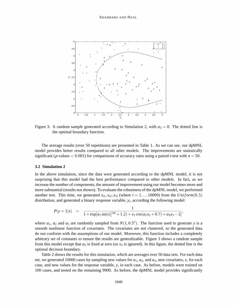
Figure 3: A random sample generated according to Simulation 2, witha3 = 0. The dotted line isthe optimal boundary function.

The average results (over 50 repetitions) are presented in Table 1. As we can see, our dpMNLmodel provides better results compared to all other models. The improvements are statisticallysignificant (p-values< 0.001) for comparisons of accuracy rates using a pairedt-test withn = 50.

3.2 Simulation 2

In the above simulation, since the data were generated according to the dpMNL model, it is notsurprising that this model had the best performance compared to other models. In fact, as weincrease the number of components, the amount of improvement using our model becomes more andmore substantial (results not shown). To evaluate the robustness of the dpMNL model, we performedanother test. This time, we generatedxi1,xi2,xi3 (wherei = 1, ...,10000) from theUni f orm(0,5)distribution, and generated a binary response variable,yi , according the following model:

P(y = 1|x) =1

1+exp[a1sin(x1.041 +1.2)+x1cos(a2x2 +0.7)+a3x3−2]

,

wherea1, a2 anda3 are randomly sampled fromN(1,0.52). The function used to generatey is asmooth nonlinear function of covariates. The covariates are not clustered, so the generated datado not conform with the assumptions of our model. Moreover, this function includes a completelyarbitrary set of constants to ensure the results are generalizable. Figure 3 shows a random samplefrom this model except thata3 is fixed at zero (sox3 is ignored). In this figure, the dotted line is theoptimal decision boundary.

Table 2 shows the results for this simulation, which are averages over 50 data sets. For each dataset, we generated 10000 cases by sampling new values fora1, a2, anda3, new covariates,x, for eachcase, and new values for the response variable,y, in each case. As before, models were trained on100 cases, and tested on the remaining 9900. As before, the dpMNL model provides significantly

1840



Baseline 61.96 (1.53) 37.99 (0.57)MNL (Maximum Likelihood) 73.58 (0.96) 68.33 (1.17)MNL 73.58 (0.97) 67.92 (1.41)qMNL 75.60 (0.98) 70.12 (1.36)Tree (Cross Validation) 73.47 (0.95) 66.94 (1.43)LSVM Linear 73.09 (0.99) 64.95 (1.71)RBF-SVM 76.06 (0.94) 68.46 (1.77)dpMNL 77.80 (0.86) 73.13 (1.26)

Table 2: Simulation 2: the average performance of models based on 50 simulated data sets. TheBaseline model assigns test cases to the class with the highest frequency inthe trainingset. Standard errors of estimates (based on 50 repetitions) are providedin parentheses.

(all p-values are smaller than 0.001) better performance compared to all other models. This time,however, the performances of qMNL and RBF-SVM are closer to the performance of the dpMNLmodel.

4. Results on Real Classification Problems

In this section, we first apply our model the problem of predicting a protein’s 3D structure (i.e.,folding class) based on its sequence. We then use our model to identify patients with Parkinson’sdisease (PD) based on their speech signals.

4.1 Protein Fold Classification

When predicting a protein’s 3D structure, it is common to presume that the number of possiblefolds is fixed, and use a classification model to assign a protein to one of these folding classes.There are more than 600 folding patterns identified in the SCOP (Structural Classification of Pro-teins) database (Lo Conte et al., 2000). In this database, proteins are considered to have the samefolding class if they have the same major secondary structure in the same arrangement with the sametopological connections.

We apply our model to a protein fold recognition data set provided by Ding and Dubchak (2001).The proteins in this data set are obtained from the PDBselect database (Hobohm et al., 1992;Hobohm and Sander, 1994) such that two proteins have no more than 35%of the sequence identityfor aligned subsequences larger than 80 residues. Originally, the resulting data set included 128unique folds. However, Ding and Dubchak (2001) selected only the 27 most populated folds (311proteins) for their analysis. They evaluated their models based on an independent sample (i.e., testset) obtained from PDB-40D (Lo Conte et al., 2000). PDB-40D contains the SCOP sequences withless than 40% identity with each other. Ding and Dubchak (2001) selected 383 representatives ofthe same 27 folds in the training set with no more than 35% identity to the training sequences. Thetraining and test data sets are available online athttp://crd.lbl.gov/ ˜ cding/protein/ .

The covariates in these data sets are the length of the protein sequence, and the percentagecomposition of the 20 amino acids. While there might exist more informative covariates to pre-dict protein folds, we use these so that we can compare the results of our model to that of Ding

1841

SHAHBABA AND NEAL

and Dubchak (2001), who trained several Support Vector Machines(SVM) with nonlinear kernelfunctions.

We centered the covariates so they have mean zero, and used the followingpriors for the MNLmodel and qMNL model (with no interactions, onlyxi andx2

i as covariates):

α j |η ∼ N(0,η2),

log(η2) ∼ N(0,22),

β jl |ξ,σl ∼ N(0,ξ2σ2l ),

log(ξ2) ∼ N(0,1),

log(σ2l ) ∼ N(−3,42).

Here, the hyperparameters for the variances of regression parameters are more elaborate than in theprevious section. One hyperparameter,σl , is used to control the variance of all coefficients,β jl

(where j = 1, ...,J), for covariatexl . If a covariate is irrelevant, its hyperparameter will tend to besmall, forcing the coefficients for that covariate to be near zero. This method, termed AutomaticRelevance Determination (ARD), has previously been applied to neural network models by Neal(1996). We also used another hyperparameter,ξ, to control the overall magnitude of allβ’s. Thisway,σl controls the relevance of covariatexl compared to other covariates, andξ controls the overallusefulness of all covariates in separating all classes. The standard deviation ofβ jl is therefore equalto ξσl .

The above scheme was also used for the dpMNL model. Note that in this model, oneσl controlsall β jlc , where j = 1, ...,J indexes classes, andc = 1, ...,C indexes the unique components in themixture. Therefore, the standard deviation ofβ jlc is ξσl νc. Here,νc is specific to each componentc, and controls the overall effect of coefficients in that component. Thatis, while σ and ξ areglobal hyperparameters common between all components,νc is a local hyperparameter within acomponent. Similarly, the standard deviation of intercepts,α jc in componentc is ητc. We usedN(0,1) as the prior forνc andτc.

We also needed to specify priors forµl andσl , the mean and standard deviation of covariatexl ,wherel = 1, ..., p. For these parameters, we used the following priors:

µlc|µ0,l ,σ0,l ∼ N(µ0,l ,σ20,l ),

µ0,l ∼ N(0,52),

log(σ20,l ) ∼ N(0,22),

log(σ2lc)|Mσ,l ,Vσ,l ∼ N(Mσ,l ,V

2σ,l ),

Mσ,l ∼ N(0,12),

log(V2σ,l ) ∼ N(0,22).

These priors make use of higher level hyperparameters to provide flexibility. For example, if thecomponents are not different with respect to covariatexl , the corresponding variance,σ2

0,l , becomessmall, forcingµlc close to their overall mean,µ0,l .

The MCMC chains for MNL, qMNL, and dpMNL ran for 10000 iterations. Simulating theMarkov chain took about 2.1 seconds per iteration (5.8 hours in total) for dpMNL and 0.5 secondsper iteration (1.4 hours in total) for MNL using a MATLAB implementation on an UltraSPARC IIImachine. Training the RBF-SVM model took about 2.5 minutes.

1842



MNL 50.0 41.2qMNL 50.5 42.1SVM (Ding and Dubchak, 2001) 49.4 -LSVM 50.5 47.3RBF-SVM 53.1 49.5dpMNL 58.6 53.0

Table 3: Performance of models based on protein fold classification data.

The results for MNL, qMNL, LSVM, RBF-SVM, and dpMNL are presented in Table 3, alongwith the results for the best SVM model developed by Ding and Dubchak (2001) on the exact samedata set. As we can see, the nonlinear RBF-SVM model that we fit has betteraccuracy than thelinear models. Our dpMNL model provides an additional improvement over theRBF-SVM model.This shows that there is in fact a nonlinear relationship between folding classes and the compositionof amino acids, and our nonlinear model could successfully identify this relationship.

4.2 Detecting Parkinson’s Disease

The above example shows that our method can potentially improve prediction accuracy, thoughof course other classifiers, such as SVM and neural networks, may dobetter on some problems.However, we believe the application of our method is not limited to simply improving predictionaccuracy—it can also be used to discover hidden structure in data by identifying subgroups (i.e.,mixture components) in the population. This section provides an example to illustrate this concept.

Neurological disorders such as Parkinson’s disease (PD) have profound consequences for pa-tients, their families, and society. Although there is no cure for PD at this time, it ispossible toalleviate its symptoms significantly, especially at the early stages of the disease (Singh et al., 2007).Since approximately 90% of patients exhibit some form of vocal impairment (Hoet al., 1998), andresearch has shown that vocal impairment could be one of the earliest indicators of onset of theillness (Duffy, 2005), voice measurement has been proposed as a reliable tool to detect and monitorPD (Sapir et al., 2007; Rahn et al., 2007; Little et al., 2008). For example, patients with PD com-monly display a symptom known asdysphonia, which is an impairment in the normal production ofvocal sounds.

In a recent paper, Little et al. (2008) show that by detectingdysphonia, we could identify pa-tients with PD. Their study used data on sustained vowel phonations from 31subjects, of whom 23were diagnosed with PD. The 22 covariates used include traditional variables, such as measures ofvocal fundamental frequency and measures of variation in amplitude of signals, as well as a novelmeasurement referred to aspitch period entropy(PPE). See Little et al. (2008) for a detailed de-scription of these variables. This data set is publicly available at UCI Machine Learning Repository(http://archive.ics.uci.edu/ml/datasets/Parkinsons ).

Little et al. (2008) use an SVM classifier with Gaussian radial basis kernelfunctions to identifypatients with PD, chosing the SVM penalty value and kernel bandwidth by an exhaustive search overa range of values. They also perform an exhaustive search to selectthe optimal subset of features(10 features were selected). Their best model provides a 91.4% (±4.4) accuracy rate based on abootstrap algorithm. This of course does not reflect the true prediction accuracy rate of the modelfor future observations since the model is trained and evaluated on the samesample. Here, we use

1843

SHAHBABA AND NEAL


MNL 85.6 (2.2) 79.1 (2.8)qMNL 86.1 (1.5) 79.7 (2.1)LSVM 87.2 (2.3) 80.6 (2.8)RBF-SVM 87.2 (2.7) 79.9 (3.2)dpMNL 87.7 (3.3) 82.6 (2.5)

Table 4: Performance of models based on detecting Parkinson’s disease. Standard errors of esti-mates (based on 5 cross-validation folds) are provided in parentheses.

Group Frequency Age Average Male Proportion

1 107 66 (0.7) 0.86 (0.03)2 12 72 (1.1) 0.83 (0.11)3 36 63 (1.8) 0.08 (0.04)4 40 65 (2.2) 0.40 (0.08)

Population 195 66 (0.7) 0.60 (0.03)

Table 5: The age average and male proportion for each cluster (i.e., mixturecomponent) identifiedby our model. Standard errors of estimates are provided in parentheses.

a 5-fold cross validation scheme instead in order to obtain a more accurate estimate of predictionaccuracy rate and avoid inflating model performance due to overfitting. Asa result, our modelscannot be directly compared to that of Little et al. (2008).

We apply our dpMNL model to the same data set, along with MNL and qMNL (no interactions,only xi andx2

i as covariates). Although the observations from the same subject are notindependent,we assume they are, as done by Little et al. (2008). Instead of selecting anoptimum subset of fea-tures, we used PCA and chose the first 10 principal components. The MCMC algorithm for MNL,qMNL, and dpMNL ran for 3000 iterations (the first 500 iterations were discarded). Simulatingthe Markov chain took about 0.7 second per iteration (35 minutes per data set) for dpMNL and0.1 second per iteration (5 minutes per data set) for MNL using a MATLAB implementation on anUltraSPARC III machine. Training the RBF-SVM model took 38 seconds foreach data set.

Using the dpMNL model, the most probable number of components in the posterior is four(note that might change from one iteration to another). Table 4 shows the average and standarderrors (based on 5-fold cross validation) of the accuracy rate and theF1 measure for MNL, LSVM,RBF-SVM, and dpMNL. (But note that the standard errors assume independence of cross-validationfolds, which is not really correct.)

While dpMNL provides slightly better results, the improvement is not statistically significant.However, examining the clusters (i.e., mixture components) identified by dpMNLreveals someinformation about the underlying structure in the data. Table 5 shows the average age of subjectsand male proportion for the four clusters (based on the most probable number of components inthe posterior) identified by our model. Note that age and gender are not available from the UCIMachine Learning Repository, and they are not included in our model. They are, however, availablefrom Table 1 in Little et al. (2008). The first two groups include substantiallyhigher percentagesof male subjects than female subjects. The average age in the second of these groups is highercompared to the first group. Most of the subjects in the third group are female (only 8% are male).

1844


The fourth group also includes more female subjects than male subjects, but the disproportionalityis not as high as for the third group.

When identifying Parkinson’s disease by detecting dysphonia, it has been shown that genderhas a confounding effect (Cnockaert et al., 2008). By grouping thedata into clusters, our modelhas identified (to some extent) the heterogeneity of subjects due to age and gender, even thoughthese covariates were not available to the model. Moreover, by fitting a separate linear model toeach component (i.e., conditioning on mixture identifiers), our model approximates the confoundingeffect of age and gender. For this example, we could have simply taken theage and gender ofsubjects from Table 1 in Little et al. (2008) and included them in our model. In many situations,however, not all the relevant factors are measured. This could resultin unobservable changes in thestructure of data. We discuss this concept in more detail elsewhere (Shahbaba, 2009).

5. Discussion and Future Directions

We introduced a new nonlinear classification model, which uses Dirichlet process mixtures to modelthe joint distribution of the response variable,y, and the covariates,x, non-parametrically. We com-pared our model to several linear and nonlinear alternative methods usingboth simulated and realdata. We found that when the relationship betweeny andx is nonlinear, our approach provides sub-stantial improvement over alternative methods. One advantage of this approach is that if the rela-tionship is in fact linear, the model can easily reduce to a linear model by usingonly one componentin the mixture. This way, it avoids overfitting, which is a common challenge in many nonlinearmodels.

We believe our model can provide more interpretable results. In many real problems, the iden-tified components may correspond to a meaningful segmentation of data. Sincethe relationshipbetweeny andx remains linear in each segment, the results of our model can be expressed as a setof linear patterns for different data segments.

Hyperparameters such asλ in RBF-SVM andγ in dpMNL can substantially influence the per-formance of the models. Therefore, it is essential to choose these parameters appropriately. ForRBF-SVM, we optimizedλ using a validation set that includes 20% of the training data. Figure 4(a) shows the effect ofλ on prediction accuracy for one data set. The value ofλ with the highestaccuracy rate based on the validation set was used to train the RBF-SVM model. The hyperparam-eters in our dpMNL model are not fixed at some “optimum” values. Instead, we use hyperpriorsthat reflect our opinion regarding the possible values of these parameters before observing the data,with the posterior for these parameters reflecting both this prior opinion and the data. Hyperpriorsfor regression parameters,β, facilitate their shrinkage towards zero if they are not relevant to theclassification task. The hyperprior for the scale parameterγ affects how many mixture componentsare present in the data. Instead of settingγ to some constant number, we allow the model to decidethe appropriate value ofγ, using a hyperprior that encourages a small number of components, butwhich is not very restrictive, and hence allowsγ to become large in the posterior if required to fitthe data. Choosing unreasonably restrictive priors could have a negative effect on model perfor-mance and MCMC convergence. Figure 4 (b) illustrates the negative effect of unreasonable priorsfor γ. For this data set, the correct number of components is two. We gradually increaseµγ, wherelog(γ) ∼ N(µγ,2), in order to put higher probability on larger values ofγ and lower probability onsmaller values. As we can see, settingµγ ≥ 4, which makes the hyperprior very restrictive, results in

1845

SHAHBABA AND NEAL

0 1 2 3 4 5 6 7 8 9 10

0.35

0.4

0.45

0.5

0.55

0.6

0.65

0.7

0.75

0.8

λ

Acc

ura

cy R

ate

−5 −4 −3 −2 −1 0 1 2 3 4 50.65

0.7

0.75

0.8

0.85

0.9

µγ

Acc

ura

cy R

ate

(So

lid L

ine)

0

10

20

30

40

50

Nu

mb

er o

f C

om

po

nen

t (D

ash

ed L

ine)

(a) (b)

Figure 4: Effects of scale parameters when fitting a data set generated according to Simulation 1.(a) The effect ofλ in the RBF-SVM model. (b) The effect of the prior on the scaleparameter,γ ∼ log-N(µγ,22), asµγ changes in the dpMNL model.

a substantial decline in accuracy rate (solid line) due to overfitting with a largenumber of mixturecomponents (dashed line).

The computational cost for our model is substantially higher compared to other methods suchas MNL and SVM. This could be a preventive factor in applying our model tosome problems.The computational cost of our model could be reduced by using more efficient methods, such asthe “split-merge” approach introduced by Jain and Neal (2007). This method uses a Metropolis-Hastings procedure that resamples clusters of observations simultaneously rather than incrementallyassigning one observation at a time to mixture components. Alternatively, it mightbe possible toreduce the computational cost by using a variational inference algorithm similar to the one proposedby Blei and Jordan (2005). In this approach, the posterior distributionP is approximated by atractable variational distributionQ, whose free variational parameters are adjusted until a reasonableapproximation toP is achieved.

We expect our model to outperform other nonlinear models such as neural networks and SVM(with nonlinear kernel functions) when the population is comprised of subgroups each with theirown distinct pattern of relationship between covariates and response variable. We also believe thatour model could perform well if the true function relating covariates to response variable containssharp changes.

The performance of our model could be negatively affected if the covariates are highly correlatedwith each other. In such situations, the assumption of diagonal covariancematrix for x adoptedby our model could be very restrictive. To capture the interdependencies between covariates, ourmodel would attempt to increase the number of mixture components (i.e., clusters). This howeveris not very efficient. To address this issue, we could use mixtures of factor analyzers, where thecovariance structure of high dimensional data is model using a small number of latent variables (seefor example, Rubin and Thayer, 2007; Ghahramani and Hinton, 1996).

In this paper, we considered only continuous covariates. Our approach can be easily extendedto situations where the covariate are categorical. For these problems, we need to replace the nor-

1846


mal distribution in the baseline,G0, with a more appropriate distribution. For example, when thecovariatex is binary, we can assumex∼ Bernoulli(µ), and specify an appropriate prior distribution(e.g.,Betadistribution) forµ. Alternatively, we can use a continuous latent variable,z, such thatµ = exp(z)/{1+ exp(z)}. This way, we can still model the distribution ofz as a mixture of nor-mals. For categorical covariates, we can either use a Dirichlet prior for the probabilities of theKcategories, or useK continuous latent variables,z1, ...,zK, and let the probability of categoryj beexp(zj)/∑K

j ′ exp(zj ′).

Throughout this paper, we assumed that the relationship betweeny andx is linear within eachcomponent of the mixture. It is possible of course to relax this assumption in order to obtain moreflexibility. For example, we can include some nonlinear transformation of the original variables(e.g., quadratic terms) in the model.

Our model can also be extended to problems where the response variable isnot multinomial.For example, we can use this approach for regression problems with continuous response,y, whichcould be assumed normal within a component. We would model the mean of this normal distributionas a linear function of covariates for cases that belong to that component.Other types of responsevariables (i.e., with Poisson distribution) can be handled in a similar way.

In the protein fold prediction problem discussed in this paper, classes were regarded as a set ofunrelated entities. However, these classes are not completely unrelated, and can be grouped intofour major structural classes known asα, β, α/β, andα + β. Ding and Dubchak (2001) show thecorresponding hierarchical scheme (Table 1 in their paper). We have previously introduced a newapproach for modeling hierarchical classes (Shahbaba and Neal, 2006, 2007). In this approach, weuse a Bayesian form of the multinomial logit model, called corMNL, with a prior that introducescorrelations between the parameters for classes that are nearby in the hierarchy. Our dpMNL modelcan be extend to classification problems where classes have a hierarchical structure (Shahbaba,2007). For this purposse, we use a corMNL model, instead of MNL, to capture the relationshipbetween the covariates,x, and the response variable,y, within each component. The results is anonlinear model which takes the hierarchical structure of classes into account.

Finally, our approach provides a convenient framework for semi-supervised learning, in whichboth labeled and unlabeled data are used in the learning process. In our approach, unlabeled datacan contribute to modeling the distribution of covariates,x, while only labeled data are used toidentify the dependence betweeny andx. This is a quite useful approach for problems where theresponse variable is known for a limited number of cases, but a large amount of unlabeled data canbe generated. One such problem is classification of web documents.

Acknowledgments

This research was supported by the Natural Sciences and EngineeringResearch Council of Canada.Radford Neal holds a Canada Research Chair in Statistics and Machine Learning.

References

E. L. Allwein, R. E. Schapire, Y. Singer, and P. Kaelbling. Reducing multiclass to binary: A unifyingapproach for margin classifiers.Journal of Machine Learning Research, 1:113–141, 2000.

1847

SHAHBABA AND NEAL

C. E. Antoniak. Mixture of Dirichlet process with applications to Bayesian nonparametric problems.Annals of Statistics, 273(5281):1152–1174, 1974.

D. Blackwell and J. B. MacQueen. Ferguson distributions via polya urn scheme.Annals of Statistics,1:353–355, 1973.

D. M. Blei and M. I. Jordan. Variational inference for dirichlet process mixtures.Bayesian Analysis,1:121–144, 2005.

D. M. Blei, A. Y. Ng, and M. I. Jordan. Latent Dirichlet allocation.Journal of Machine LearningResearch, 3:993–1022, January 2003.

L. Breiman, J. Friedman, R. A. Olshen, and C. J. Stone.Classification and Regression Trees.Chapman and Hall, Boca Raton, 1993.

C. A. Bush and S. N. MacEachern. A semi-parametric Bayesian model for randomized blockdesigns.Biometrika, 83:275–286, 1996.

B. Cai and D. B. Dunson. Bayesian covariance selection in generalizedlinear mixed models.Bio-metrics, 62:446–457, 2006.

L. Cnockaert, J. Schoentgen, P. Auzou, C. Ozsancak, L. Defebvre, and F. Grenez. Low-frequencyvocal modulations in vowels produced by parkinsonian subjects.Speech Communication, 50(4):288–300, 2008.

M. J. Daniels and R. E. Kass. Nonconjugate Bayesian estimation of covariance matrices and itsuse in hierarchical models.Journal of the American Statistical Association, 94(448):1254–1263,1999.

C. H. Q. Ding and I. Dubchak. Multi-class protein fold recognision using support vector machinesand neural networks.Bioinformatics, 17(4):349–358, 2001.

J. R. Duffy.Motor Speech Disorders: Substrates, Differential Diagnosis and Management. ElsevierMosby, St. Louis, Mo., 2nd edition, 2005.

M. D. Escobar and M. West. Bayesian density estimation and inference using mixtures.Journal ofAmerican Statistical Society, 90:577–588, 1995.

T. S. Ferguson. A Bayesian analysis of some nonparametric problems.Annals of Statistics, 1:209–230, 1973.

T. S. Ferguson.Recent Advances in Statistics, Ed: Rizvi, H. and Rustagi, J., chapter Bayesiandensity estimation by mixtures of normal distributions, pages 287–302. Academic Press, NewYork, 1983.

J. Furnkranz. Round robin classification.Journal of Machine Learning Research, 2:721–747, 2002.ISSN 1533-7928.

Z. Ghahramani and G. E. Hinton. The EM algorithm for mixtures of factor analyzers. Technicalreport, Technical Report CRG-TR-96-1, Department of Computer Science, University of Toronto,1996.

1848


A. K. Ho, R. Iansek, C. Marigliani, J. L. Bradshaw, and S. Gates. Speech impairment in a largesample of patients with Parkinson’s disease.Behavioural Neurology, 11:131–137, 1998.

U. Hobohm and C. Sander. Enlarged representative set of proteins.Protein Science, 3:522–524,1994.

U. Hobohm, M. Scharf, R. Schneider, and C. Sander. Selection of a representative set of structurefrom the brookhaven protein bank.Protein Science, 1:409–417, 1992.

C. W. Hsu and C. J. Lin. A comparison of methods for multi-class support vector machines.IEEETransactions on Neural Networks, 13:415–425, 2002.

R. A. Jacobs, M. I. Jordan, S. J. Nowlan, and G. E. Hinton. Adaptivemixtures of local experts.Neural Computation, 3(1):79–87, 1991.

S. Jain and R. M. Neal. Splitting and merging components of a nonconjugate Dirichlet processmixture model (with discussion).Bayesian Analysis, 2:445–472, 2007.

M. A. Little, P. E. McSharry, E. J. Hunter, J. Spielman, and L. O. Ramig. Suitability of dyspho-nia measurements for telemonitoring of Parkinson’s disease.IEEE Transactions on BiomedicalEngineering, (in press), 2008.

L. Lo Conte, B. Ailey, T.J.P Hubbard, S. E. Brenner, A.G. Murzing, andC. Chothia. Scop: astructural classification of protein database.Nucleic Acids Research, 28:257–259, 2000.

S. N. MacEachern and P. Muller. Estimating mixture of Dirichlet process models.Journal ofComputational and Graphcal Statistics, 7:223–238, 1998.

E. Meeds and S. Osindero. An alternative infinite mixture of Gaussian process experts.Advancesin Neural Information Processing Systems, 18:883, 2006.

P. Muller, A. Erkanli, and M. West. Bayesian curve fitting using multivariate mormalmixtures.Biometrika, 83(1):67–79, 1996.

R. M. Neal. Markov chain sampling methods for Dirichlet process mixture models. Journal ofComputational and Graphical Statistics, 9:249–265, 2000.

R. M. Neal. Slice sampling.Annals of Statistics, 31(3):705–767, 2003.

R. M. Neal. Probabilistic Inference Using Markov Chain Monte Carlo Methods. Technical ReportCRG-TR-93-1, Department of Computer Science, University of Toronto, 1993.

R. M. Neal. Bayesian Learning for Neural Networks. Lecture Notes in Statistics No. 118, NewYork: Springer-Verlag, 1996.

D. A. Rahn, M. Chou, J. J. Jiang, and Y. Zhang. Phonatory impairment in Parkinson’s disease:evidence from nonlinear dynamic analysis and perturbation analysis.(Clinical report).Journal ofVoice, 21:64–71, 2007.

C. E. Rasmussen and Z. Ghahramani. Infinite mixtures of Gaussian process experts. InAdvancesin Neural Information Processing Systems 14, page 881. MIT Press, 2002.

1849

SHAHBABA AND NEAL

D. Rubin and D. Thayer. EM algorithms for ML factor analysis.Pshychometrika, 47(1):69–76,2007.

S. Sapir, J. L. Spielman, L. O. Ramig, B. H. Story, and C. Fox. Effects ofintensive voice treatment(the Lee Silverman Voice Treatment [lsvt]) on vowel articulation in dysarthricindividuals withidiopathic Parkinson disease: Acoustic and perceptual findings.Journal of Speech, Language,and Hearing Research, 50(4):899–912, 2007.

B. Shahbaba. Discovering hidden structures using mixture models: Application to nonlinear timeseries processes.Studies in Nonlinear Dynamics & Econometrics, 13(2):Article 5, 2009.

B. Shahbaba.Improving Classification Models When a Class Hierarchy is Available. PhD thesis,Biostatistics, Public Health Sciences, University of Toronto, 2007.

B. Shahbaba and R. M. Neal. Improving classification when a class hierarchy is available using ahierarchy-based prior.Bayesian Analysis, 2(1):221–238, 2007.

B. Shahbaba and R. M. Neal. Gene function classification using Bayesianmodels with hierarchy-based priors.BMC Bioinformatics, 7:448, 2006.

N. Singh, V. Pillay, and Y. E. Choonara. Advances in the treatment of Parkinson’s disease.Progressin Neurobiology, 81:29–44, 2007.

I. Ulusoy and C. M. Bishop. Generative versus discriminative methods for object recognition. InCVPR ’05: Proceedings of the 2005 IEEE Computer Society Conferenceon Computer Vision andPattern Recognition (CVPR’05) - Volume 2, pages 258–265, Washington, DC, USA, 2005. IEEEComputer Society.

V. N. Vapnik. The Nature of Statistical Learning Theory. Springer-Verlag New York, Inc., NewYork, NY, USA, 1995. ISBN 0-387-94559-8.

S. Waterhouse, D. MacKay, and T. Robinson. Bayesian methods for mixtures of experts. InAd-vances in Neural Information Processing Systems 8, page 351. MIT Press, 1996.

1850

nonlinear models using dirichlet process mixtures - journal of

Documents