SEPARATION OF POST-NONLINEAR MIXTURES USING ACE AND TEMPORALDECORRELATION

Andreas Ziehe���

, Motoaki Kawanabe�, Stefan Harmeling

�and Klaus-Robert Muller

��� ��GMD FIRST.IDA, Kekulestr. 7, 12489 Berlin, Germany�

University of Potsdam, Am Neuen Palais 10, 14469 Potsdam, Germany�ziehe,nabe,harmeli,klaus � @first.gmd.de

ABSTRACT

We propose an efficient method based on the concept ofmaximal correlation that reduces the post-nonlinear blindsource separation problem (PNL BSS) to a linear BSS prob-lem. For this we apply the Alternating Conditional Expec-tation (ACE) algorithm – a powerful technique from non-parametric statistics – to approximately invert the (post-)non-linear functions. Interestingly, in the framework of the ACEmethod convergence can be proven and in the PNL BSSscenario the optimal transformation found by ACE will co-incide with the desired inverse functions. After the non-linearities have been removed by ACE, temporal decorrela-tion (TD) allows us to recover the source signals. An ex-cellent performance underlines the validity of our approachand demonstrates the ACE-TD method on realistic exam-ples.

1. INTRODUCTION

Blind source separation (BSS) research has mainly beenfocused on variants of linear ICA and temporal decorrela-tion methods (see e.g. [14, 6, 5, 7, 1, 2, 13, 29, 22, 12]).Linear BSS assumes that at time � each component ��� �� of the observed � -dimensional data vector ��� �� is a linearcombination of ����� statistically independent signals:��� �� ��������� ��! �#"�� � �� (e.g. [12]). The source signals "$� � �� are unknown, as are the coefficients ! � of the mixing ma-trix % . The goal is therefore to estimate both unknownsfrom the observed signals �&� �� , i.e. a separating matrix 'and signals ()� �� ���'*�&� �� that estimate +,� �� .

However, non-linearities that distort the mixed signals,pose a challenging problem for “conventional” BSS meth-ods, where the mixing model is linear instantaneous or con-volutive. The general nonlinear mixing model is (cf. [12])

- � �� ��/.10�23� �� 54 (1)6To whom correspondence should be addressed.

This work was partly supported by the EU under contract IST-1999-14190 – BLISS.

where . is an arbitrary nonlinear transformation (at least ap-proximately invertible). An important special case are post-nonlinear (PNL) mixtures

- � �� 7�/.108%923� �� 54�: (2)

where . is an invertible nonlinear function that operatescomponentwise and % is a linear mixing matrix. Becausethis PNL model, which has been introduced by Taleb andJutten [25], is an important subclass with interesting prop-erties it attracted the interest of several researchers [25, 15,27]. Furthermore it is often an adequate modelling of real-world physical systems, where nonlinear transfer functionsappear; e.g. in the fields of telecommunications or biomedi-cal data recording sensors can have a nonlinear characteris-tics.

;<= >?

@ A BDC�E�F B,GHBH@ A BDC�EIFJ A KLA BHM N A OQPRGHFSP A GHB

T UV

B,GHBH@ A BDCWEIF @ A BDC�EIFP F�EIBXO�YZGHF J [ B J A KLA BHM\

Fig. 1: Building blocks of the PNL mixing model and the separa-tion system.

Algorithmic solutions of eq.(2) have used e.g. self-or-ganizing maps [20, 18], extensions of GTM [21], neuralnetworks [27, 19], parametric sigmoidal functions [16] orensemble learning [26] to approximate the nonlinearity .(or its inverse ] ). Also kernel based methods were tried onvery simple toy signals [8] and more recently also on real-world data using temporal decorrelation in feature space[10]. Note, that most existing methods (except [10]) areof high computational cost and depending on the algorithmare prone to run into local minima.

In our approach to the PNL BSS problem we first ap-proximately invert the post-nonlinearity using the ACE al-gorithm (estimating ] ) and then apply a standard BSS tech-

433

nique [3, 29] that relies on temporal decorrelation (estimat-ing the unmixing matrix ' ) (cf. Fig.1). By virtue of theACE framework, which is briefly introduced in subsection2.2, we prove that the algorithm converges to the correct in-verse nonlinearities – provided that they exist. Some imple-mentation issues are discussed and numerical simulationsillustrating the method are described in section 3. Finally aconclusion is given in section 4.

2. METHODS

For the sake of simplicity we introduce our method for the�����case. The extension to the general case is easily pos-

sible, but omitted for better readability.

2.1. Problem statement

Let us consider the�

dimensional post-nonlinear mixingmodel: � ��� � 0�� ���L" �� � �� "� 4 ��� 0�� ��L" �� � "� 4where " � and "� are independent source signals, that aretemporally correlated, � and are the observed signals,% � 0��D � 4 is the mixing matrix and � � and � are the com-ponentwise nonlinear transformations which are invertible.

Obviously, any attempt to separate such a mixture by alinear BSS algorithm will fail, unless one could invert thefunctions � � and � at least approximately. In this work wepropose that this can be achieved by maximizing the corre-lation

corr 0�� � 05 � 4�:�� 05 4I4 (3)

with respect to nonlinear functions � � and � . This means,we want to find transformations � � and � of the observedsignals such that the relationship between the transformedvariables becomes linear. Intuitively speaking, the relation-ship is linear, if the signals are aligned in a scatterplot, i.e. ifthey are maximally correlated. Under certain conditions thatwe will state in detail later, this problem is solved by theACE method that finds so called optimal transformations ����and ��� which maximize eq.(3). One can prove existenceand uniqueness of those optimal transformations and it canbe shown that the ACE algorithm, which is described in thefollowing, converges to these solutions (cf. [4]).

2.2. ACE algorithm

The ACE algorithm is an iterative procedure for finding theoptimal nonlinear functions � �� and � � . The starting point isthe observation that for fixed � � the optimal � is given by

� 05 4&������� � 05 � 4�� �� :and conversely, for fixed � the optimal � � is

� � 05 � 4&������� 05 4�� �����

The key idea of the ACE algorithm is therefore to computealternately the respective conditional expectations. To avoidtrivial solutions one normalizes � � 05 � 4 in each step by using

the function norm � ����� �! �#"$����� � �% �'& . The algorithm fortwo variables is summarized below. It is also possible toextend the procedure to the multivariate case, however, forfurther details we refer to [11, 4].

Algorithm 1 The ACE algorithm for two variables� initialize ��)( *,+� 05 � 4- ��. � � � � �repeat�)(0/21 � + 05 43-4�����)(0/2+� 05 � 45�# ��6�)(0/21 � +� 05 � 43-4�����)(0/21 � + 05 45�# ����)(0/21 � +� 05 � 43- 6�)(0/21 � +� 05 � 4 . � � 6�)(0/21 � +� 05 � 4�� �until ����� � 05 � 4879� 05 4 � fails to decrease

An important point in the implementation of this algo-rithm is the estimation of the conditional expectations fromthe data. Usually, the conditional expectations are com-puted by data smoothing for which numerous techniquesexist (cf. [4, 9]). Care has to be taken to balance the trade-off between the fidelity to the data against the smoothness ofthe estimated curve. Our implementation utilizes a nearestneighbor smoothing that applies a simple moving averagefilter to appropriately sorted data.

By applying �)�� and ��� to the mixed signals � and weremove the effect of the nonlinear functions � � and � . Inthe following we will substantiate this claim more formally.We show for : � �;� ���$" �<� � �� "� and : �=� ��L" �<� � #"�that ���� and ��� obtained from the ACE procedure are the de-sired inverse functions for the case that : � and : are jointlynormal distributed, with other words we prove the followingrelationship: >

�� 0�: � 4? �@���� 0A� � 0�: � 4I4B�: �>� 0�: 4? �@� � 0A� 0�: 4I4<B�: C� (4)

Almost all work for the proof has already been done inProposition 5.4. and Theorem 5.3. of [4] which – by notic-ing that the correlation of two signals does not change, if wescale one or both signals – implies:

���� 05 � 4B�������� 05 4�� ������ 05 4B��������� 05 � 4�� ����Note that the conditional expectation ����� � 05 4�� ��� is

a function of � and the expectation is taken with respect to , analogously for the second expression.Since ���� 05 � 4 �

>�� 0�: � 4 and ��� 05 4 �

>� 0�: 4 , furthermore � ��� � 0�: � 4 and ��� 0�: 4 we get:>

�� 0�: � 4B����>� 0�: 4�� � � 0�: � 4 �>

� 0�: 4<BD���>�� 0�: � 4�� � 0�: 4 ���

434

Because � � and � are invertible functions they can be omit-ted in the condition of the conditional expectation, leadingus to:

>�� 0�: � 4B����

>� 0�: 4�� : ���>

� 0�: 4B����>�� 0�: � 4�� : C��� (5)

Assuming that the vector 0�: � : : 4�� is normally distributedand the correlation corr 0�: � : : 4 does not vanish, a straight-forward calculation shows

����: � : ��� B�: �����: � � : C� B�: ��This means that : � and : satisfy eq. (5), which then imme-diately implies our claim eq. (4). Fortunately, in our appli-cation the above assumptions are usually fulfilled becausemixed signals are more Gaussian and more correlated thanunmixed signals. On the other hand, even if the assump-tions are not perfectly met, experiments show that the ACEalgorithm still equalizes the nonlinearities well.

Summarizing the key idea, by searching for nonlineartransformations, that maximize the linear correlations be-tween the non-linearly transformed observed variables, wecan approximate the inverses of the post-nonlinearities.

2.3. Source separation

For a separation of the signals one could in principle ap-ply any BSS technique, capable of solving the now approx-imately linear problem. However, experiments show thatonly second-order methods which use temporal informa-tion are sufficiently robust to reliably recover the sources.Therefore we use TDSEP, an implementation based on thesimultaneous diagonalization of several time-delayed corre-lation matrices for the blind identification of the unmixingmatrix ' (cf. [3, 29, 28]).

3. NUMERICAL SIMULATIONS

To demonstrate the performance of the proposed method weapply our algorithm to several post-nonlinear mixtures, bothinstantaneous and convolutive.

The first data set consists of Gaussian AR-processes ofthe form:

" ���

� � �� � " �� � ��� I: ��� : ����� :I��: (6)

where � is white Gaussian noise with mean zero and vari-ance �

. For the experiment we choose �

�� , ���� ,� � �and generate 2000 data points.

We use a� � �

mixing matrix to get linearly mixed sig-nals � and apply strong nonlinear distortions

� � �� � � � 0�: � � �� 54��D:��� � �� �: (7)

� �� � � 0�: � �� 54���������� 0����: � �� 54�:

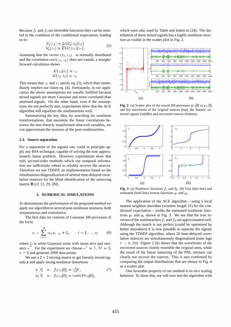
which were also used by Taleb and Jutten in [24]. The dis-tribution of these mixed signals has a highly nonlinear struc-ture as visible in the scatter plot in Fig. 2.

200 400 600 800 1000 1200 1400 1600 1800 2000

2

1

s

200 400 600 800 1000 1200 1400 1600 1800 2000

2

1

u lin

200 400 600 800 1000 1200 1400 1600 1800 2000

2

1

u nonl

in

−1 0 1−2

−1.5

−1

−0.5

0

0.5

1

1.5

2

x2

x 1

(a) (b)

Fig. 2: (a) Scatter plot of the mixed AR-processes ( � �"! #%$ vs ��&�! #%$ )and (b) waveforms of the original sources (top), the linearly un-mixed signals (middle) and recovered sources (bottom).

−1 −0.5 0 0.5 1−1

−0.5

0

0.5

1

f1

−1 −0.5 0 0.5 1−1

−0.5

0

0.5

1f2

(a)

−4 −2 0 2 4−2

−1

0

1

2

g1

−1.5 −1 −0.5 0 0.5 1 1.5−1

−0.5

0

0.5

1g

2

(b)

Fig. 3: (a) Nonlinear functions '(� and ')& . (b) True (thin line) andestimated (bold line) inverse functions *�� and *(& .

The application of the ACE algorithm – using a localnearest neighbor smoother (window length 31) for the con-ditional expectation – yields the estimated nonlinear func-tions � � and � shown in Fig. 3. We see that the true in-verses of the nonlinearities � � and � are approximated well.Although the match is not perfect (could be optimized bybetter smoothers) it is now possible to separate the signalsusing the TDSEP algorithm, where 20 time-delayed corre-lation matrices are simultaneously diagonalized (time lags+ ��� � � � � ). Figure 2 (b) shows that the waveforms of therecovered sources closely resemble the original ones, whilethe result of the linear unmixing of the PNL mixture canclearly not recover the sources. This is also confirmed bycomparing the output distributions that are shown in Fig. 4as a scatter plot.

One favorable property of our method is its nice scalingbehavior. To show this, we will now test the algorithm with

435

−0.05 0 0.05−0.1

−0.05

0

0.05

0.1

u1

u 2

Fig. 4: Scatter plot of the output distribution of a linear (‘+’) andthe proposed nonlinear ACE-TD algorithm (‘.’).

natural audio sources, where the input data set consists of 4sound signals with

� � : � � � data points each. For this casewe apply the multivariate version of the ACE algorithm,which computes the optimal functions by maximizing thegeneralized correlation criterion corr 0�� � 05 � 4�: � � / �! � / 05 / 4I4 .For details of the implementation we refer to [4, 11, 9]. Asin the first experiment, these source signals were mixed bya linear model �3� �� �� % +,� �� , with a random (

� � �) matrix% . After the linear mixing the following nonlinearities were

applied:

� � 0�: � 4 � : �� � � �� : ��� 0�: 4 � � � ��: <� ���,�>0 ��: 4� � 0�: � 4 � ���,�

>0 � : � 4���,0�:��#4 � : �� �

(8)

Figure 5 shows the results of the separation using ACE-TD(smoothing window length 51) and TDSEP ( + � � � � � � ). Weobserve again a very good separation performance that isquantified by calculating the correlation coefficients (shownin table 1) between the source signals and the extractedcomponents. This is also confirmed by listening to the sep-arated audio signals, were we perceive almost no crosstalk,although the noise level is slightly increased (cf. the silentparts of signal 2 in Fig. 5).

The third experiment gives an example for the applica-tion of our method to convolutive mixtures with a PNL dis-tortion. We deliberately distorted real-room recordings1 ofspeech and background music made by Lee [17] with non-linear transfer functions as in our first example (cf. eq.(7)).For the separation we apply a convolutive BSS algorithmof Parra et al. that requires only second-order statistics by

1Available on the internet viahttp://sloan.salk.edu/˜tewon/Blind/blind audio.html

4

3

2

1

4

3

2

1

4

3

2

1

0 20000

(a)

(b)

(c)

20000

20000

0

0

Fig. 5: Four channel audio dataset: (a) waveforms of the originalsources, (b) linearly unmixed signals with TDSEP and (c) recov-ered sources using ACE-TD.

exploiting the non-stationarity of the signals [23]. Whilean unmixing of the distorted recordings obviously fails, wecould achieve a good separation after the unsupervised lin-earization by the ACE procedure (cf. Fig. 6).

4. DISCUSSION AND CONCLUSION

In this work we proposed a simple technique for the blindseparation of linear mixtures with a post-nonlinear distor-tion. The main ingredients of our algorithm, which we callACE-TD, are: first, a search for nonlinear transformationsthat maximize the linear correlations between transformedvariables and which approximate the inverses of the PNLs.This search can be done highly efficient by the ACE tech-nique [4] from non-parametric statistics, that performs analternating estimation of conditional expectations by smooth-ing of scatter plots. Effectively, this nonlinear modelingprocedure solves the PNL mixture problem by transform-ing it back into a linear one. Therefore, second, a temporaldecorrelation BSS algorithm (e.g. [3, 29]) can be applied.

436

TDSEP� � � �

�� �" � 0.10 0.56 0.31 -0.13"� -0.01 0.26 0.02 0.47"

� 0.06 0.12 0.76 -0.05" � -0.07 0.66 -0.21 0.11

ACE-TD" � 0.97 -.01 -.005 0.03"� 0.03 0.94 -0.02 -0.005"� 0.01 0.07 0.95 -0.007" � 0.04 0.002 0.001 0.96

Table 1: Correlation coefficients for the signals shown in Fig. 5

Clearly, ACE is not limited to the�3���

case but itscales naturally to the � � � case for which an algorith-mic description can be found in [4, 9]. Moreover, the algo-rithm can make beneficial use of additional sensors in theoverdetermined BSS case as then the joint distribution of�3� �� becomes more and more Gaussian, which is beneficialfor ACE. Furthermore, our method works also for convolu-tive mixtures, which is attractive for real-room BSS, wherenonlinear transfer functions of the sensors (microphones)or amplifiers would impede a proper separation. Conclud-ing, the proposed framework gives a simple algorithm ofhigh efficiency with a solid theoretical background for sig-nal separation in applications with a PNL distortion, that areof importance e.g. in real-world sensor technology.

Future research will be concerned with a better tuningof the smoothers which are essential in the ACE algorithmto the PNL blind source separation scenario.

5. REFERENCES

[1] S.-I. Amari, A. Cichocki, and H.H. Yang. A new learn-ing algorithm for blind source separation. In Advancesin Neural Information Processing Systems 8, pages757–763. MIT Press, 1996.

[2] A.J. Bell and T.J. Sejnowski. An information-maximization approach to blind separation and blinddeconvolution. Neural Computation, 7:1129–1159,1995.

[3] A. Belouchrani, K. Abed Meraim, J.-F. Cardoso, andE. Moulines. A blind source separation techniquebased on second order statistics. IEEE Trans. on Sig-nal Processing, 45(2):434–444, 1997.

[4] L. Breiman and J. H. Friedman. Estimating optimaltransformations for multiple regression and correla-tion. Journal of the American Statistical Association,80(391):580–598, September 1985.

2

1

2

1

2

1

2

1

2

1

(a)

(b)

(c)

(d)

(e)

Fig. 6: Two channel auido dataset: (a) waveforms of the recorded(undistorted) microphone signals, (b) observed PNL distorted sig-nals, (c) result of ACE, (d) recovered sources using ACE and a con-volutive BBS algorithm and (e) for comparison convolutive BSSseparation result for undistorted signals from (a).

[5] J.-F. Cardoso and A. Souloumiac. Blind beamform-ing for non Gaussian signals. IEE Proceedings-F,140(6):362–370, 1993.

[6] P. Comon. Independent component analysis—a newconcept? Signal Processing, 36:287–314, 1994.

[7] G. Deco and D. Obradovic. Linear redundancy reduc-tion learning. Neural Networks, 8(5):751–755, 1995.

[8] C. Fyfe and P. L. Lai. ICA using kernel canonical cor-relation analysis. In Proc. Int. Workshop on Indepen-dent Component Analysis and Blind Signal Separation(ICA2000), pages 279–284, Helsinki, Finland, 2000.

[9] W. Hardle. Applied Nonparametric Regression. Cam-bridge University Press, Cambridge, 1990.

437

[10] S. Harmeling, A. Ziehe, M. Kawanabe, B. Blankertz,and K.-R. Muller. Nonlinear blind source separationusing kernel feature spaces. submitted to ICA 2001.

[11] T.J. Hastie and R.J. Tibshirani. Generalized AdditiveModels, volume 43 of Monographs on Statistics andApplied Probability. Chapman & Hall, London, 1990.

[12] A. Hyvarinen, J. Karhunen, and E. Oja. IndependentComponent Analysis. Wiley, 2001.

[13] A. Hyvarinen and E. Oja. A fast fixed-point algorithmfor independent component analysis. Neural Compu-tation, 9(7):1483–1492, 1997.

[14] C. Jutten and J. Herault. Blind separation of sources,part I: An adaptive algorithm based on neuromimeticarchitecture. Signal Processing, 24:1–10, 1991.

[15] T.-W. Lee, B.U. Koehler, and R. Orglmeister. Blindsource separation of nonlinear mixing models. In Neu-ral Networks for Signal Processing VII, pages 406–415. IEEE Press, 1997.

[16] T-W. Lee, B.U. Koehler, and R. Orglmeister. Blindsource separation of nonlinear mixing models. IEEEInternational Workshop on Neural Networks for Sig-nal Processing, pages 406–415, September 1997.

[17] T-W. Lee, A. Ziehe, R. Orglmeister, and T. J. Se-jnowski. Combining time-delayed decorrelation andICA: Towards solving the cocktail party problem. InProc. ICASSP98, volume 2, pages 1249–1252, Seattle,1998.

[18] J. K. Lin, D. G. Grier, and J. D. Cowan. Faithful rep-resentation of separable distributions. Neural Compu-tation, 9(6):1305–1320, 1997.

[19] G. Marques and L. Almeida. Separation of nonlin-ear mixtures using pattern repulsion. In Proc. Int.Workshop on Independent Component Analysis andSignal Separation (ICA’99), pages 277–282, Aussois,France, 1999.

[20] P. Pajunen, A. Hyvarinen, and J. Karhunen. Nonlin-ear blind source separation by self-organizing maps.In Proc. Int. Conf. on Neural Information Processing,pages 1207–1210, Hong Kong, 1996.

[21] P. Pajunen and J. Karhunen. A maximum likelihoodapproach to nonlinear blind source separation. InProceedings of the 1997 Int. Conf. on Artificial Neu-ral Networks (ICANN’97), pages 541–546, Lausanne,Switzerland, 1997.

[22] P. Pajunen and J. Karhunen, editors. Proc. of the2nd Int. Workshop on Independent Component Anal-ysis and Blind Signal Separation, Helsinki, Finland,June 19-22, 2000. Otamedia, 2000.

[23] L. Parra and C. Spence. Convolutive blind sourceseparation of non-stationary sources. IEEE Trans. onSpeech and Audio Processing, 8(3):320–327, May2000. US Patent US6167417.

[24] A. Taleb and C. Jutten. Batch algorithm for source sep-aration in post-nonlinear mixtures. In Proc. First Int.Workshop on Independent Component Analysis andSignal Separation (ICA’99), pages 155–160, Aussois,France, 1999.

[25] A. Taleb and C. Jutten. Source separation in post-nonlinear mixtures. IEEE Trans. on Signal Process-ing, 47(10):2807–2820, 1999.

[26] H. Valpola, X. Giannakopoulos, A. Honkela, andJ. Karhunen. Nonlinear independent component anal-ysis using ensemble learning: Experiments and dis-cussion. In Proc. Int. Workshop on IndependentComponent Analysis and Blind Signal Separation(ICA2000), pages 351–356, Helsinki, Finland, 2000.

[27] H. H. Yang, S. Amari, and A. Cichocki. Information-theoretic approach to blind separation of sources innon-linear mixture. Signal Processing, 64(3):291–300, 1998.

[28] A. Yeredor. Blind separation of gaussian sourcesvia second-order statistics with asymptotically optimalweighting. IEEE Signal Processing Letters, 7(7):197–200, 2000.

[29] A. Ziehe and K.-R. Muller. TDSEP–an efficientalgorithm for blind separation using time structure.In Proc. Int. Conf. on Artificial Neural Networks(ICANN’98), pages 675–680, Skovde, Sweden, 1998.

438