estimation in mixed models with dirichlet process …jrojo/4th-lehmann/slides/casella.pdfestimation...

The Fourth Erich L. Lehmann Symposium May 9 - 12, 2011

Estimation in Mixed Modelswith

Dirichlet Process Random EffectsBoth Sides of the Story

George Casella Chen Li

Department of Statistics Department of StatisticsUniversity of Florida University of Florida

Minjung Kyung Jeff GillCenter for Applied Statistics Center for Applied Statistics

Washington University Washington University

Supported by NSF Grants: SES-0958982 & SES-0959054.

Estimation in Dirichlet Process Random Effects Models: Introduction [1]

Introduction

◮ The Beginning Prior distributions in the social sciences

◮ Transition After the data analysis: model properties

◮ Dirichlet ProcessRandom Effects

Likelihood, subclusters, precision parameter

◮ MCMC Parameter expansion, convergence, optimality

◮ Example Scottish election, normal random effects

◮ Some Theory Why are the intervals shorter?

◮ ClassicalMixed Models

OLS, BLUE

◮ Conclusions And other remarks

Estimation in Dirichlet Process Random Effects Models: Introduction [2]

———But First———Here is the Big Picture

◮ Usual Random Effects Model

Y|ψ ∼ N(Xβ + ψ, σ2I), ψi ∼ N(0, τ 2)

⊲ Subject-specific random effect

◮ Dirichlet Process Random Effects Model

Y|ψ ∼ N(Xβ + ψ, σ2I), ψi ∼ DP(m,N(0, τ 2))

◮ Results in

⊲ Fewer Assumptions

⊲ Better Estimates

⊲ Shorter Credible Intervals

⊲ Straightforward Classical Estimation

Estimation in Dirichlet Process Random Effects Models: How this all started [3]

How This All StartedThe Use of Prior Distributions in the Social Sciences

Can more flexiblepriors help usrecover latenthierarchicalinformation?

◮ When do priors matter in social science research?

◮ How to specify known prior information?

◮ Bayesian social scientists like uninformed priors

◮ Reviewers often skeptical about informed priors

◮ Survey of Political Executives (Gill and Casella 2008 JASA)

⊲ Outcome Variable: stress

⊲ surrogate for self-perceived effectiveness and job-satisfaction

⊲ five-point scale from “not stressful at all” to “very stressful.”

⊲ Ordered probit model

Estimation in Dirichlet Process Random Effects Models: How this all started [4]

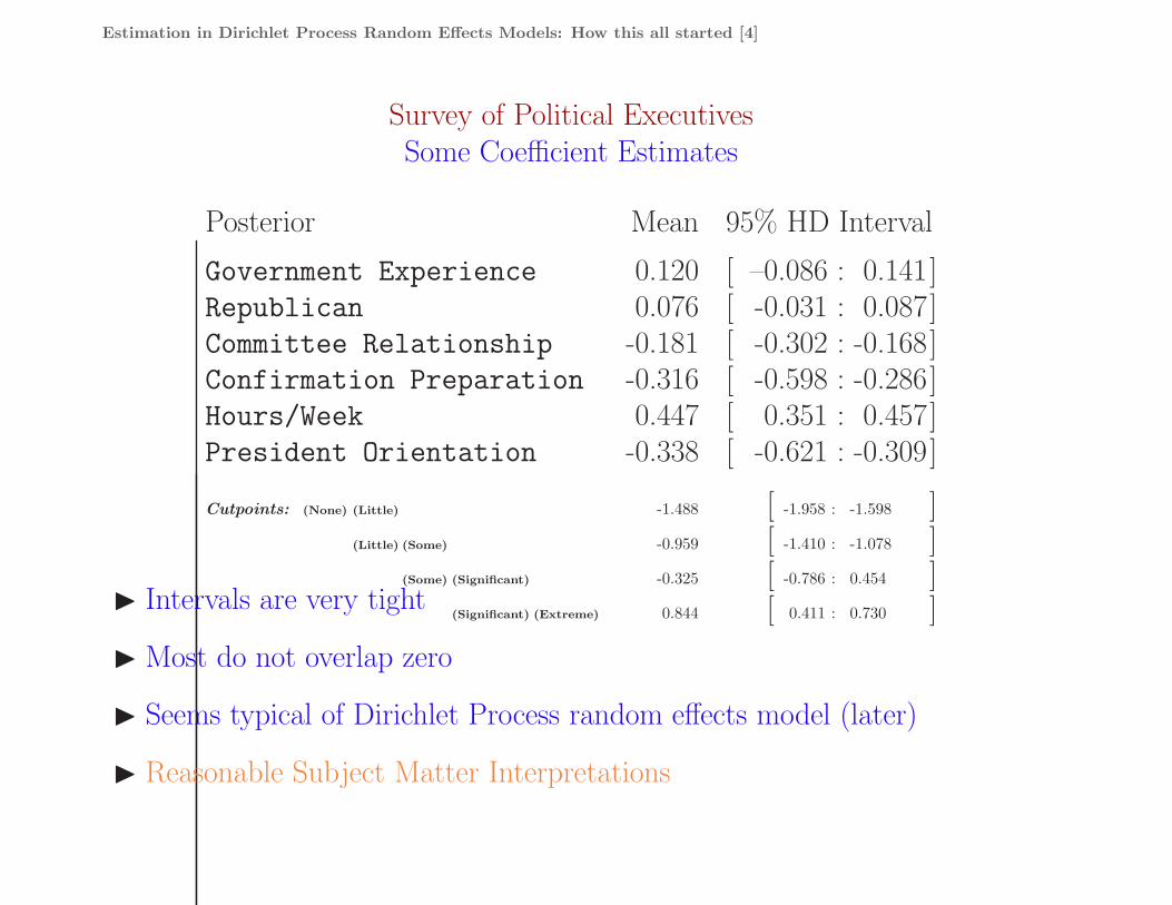
Survey of Political ExecutivesSome Coefficient Estimates

Posterior Mean 95% HD Interval

Government Experience 0.120 [ –0.086 : 0.141]Republican 0.076 [ -0.031 : 0.087]Committee Relationship -0.181 [ -0.302 : -0.168]Confirmation Preparation -0.316 [ -0.598 : -0.286]Hours/Week 0.447 [ 0.351 : 0.457]President Orientation -0.338 [ -0.621 : -0.309]

Cutpoints: (None) (Little) -1.488 [ -1.958 : -1.598 ](Little) (Some) -0.959 [ -1.410 : -1.078 ]

(Some) (Significant) -0.325 [ -0.786 : 0.454 ](Significant) (Extreme) 0.844 [ 0.411 : 0.730 ]◮ Intervals are very tight

◮ Most do not overlap zero

◮ Seems typical of Dirichlet Process random effects model (later)

◮ Reasonable Subject Matter Interpretations

Estimation in Dirichlet Process Random Effects Models: Motivation [5]

TransitionWhat Did We Learn?

AnalyzingSocial Science Data

Understandingthe Methodology

◮ Dirichlet Process Random Effects Models

⊲ Accepted by Social Scientists

⊲ Computationally Feasible

⊲ Provides good estimates

◮ “Off the shelf ” MCMC ⊲ can we do better?

◮ Precision parameter m ⊲ arbitrarily fixed

◮ Answers insensitive to m???

◮ Next: Better understanding of MCMC and estimation of m.

◮ Performance evaluations and wider applications

Estimation in Dirichlet Process Random Effects Models: Details of the Model [6]

A Dirichlet Process Random Effects ModelEstimating the Dirichlet Process Parameters

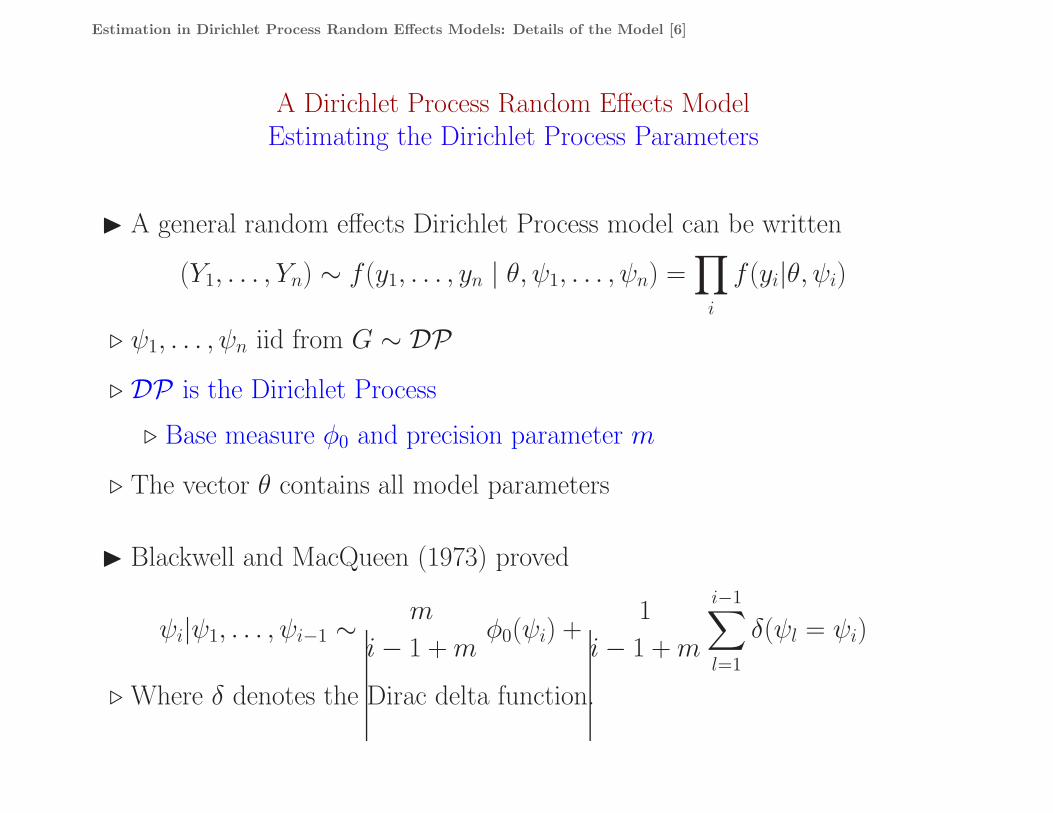
◮ A general random effects Dirichlet Process model can be written

(Y1, . . . , Yn) ∼ f(y1, . . . , yn | θ, ψ1, . . . , ψn) =∏

i

f(yi|θ, ψi)

⊲ ψ1, . . . , ψn iid from G ∼ DP

⊲ DP is the Dirichlet Process

⊲ Base measure φ0 and precision parameter m

⊲ The vector θ contains all model parameters

◮ Blackwell and MacQueen (1973) proved

ψi|ψ1, . . . , ψi−1 ∼m

i− 1 +mφ0(ψi) +

1

i− 1 +m

i−1∑

l=1

δ(ψl = ψi)

⊲ Where δ denotes the Dirac delta function.


Some Distributional Structure

◮ Freedman (1963), Ferguson (1973, 1974) and Antoniak (1974)

⊲ Dirichlet process prior for nonparametric G

⊲ Random probability measure on the space of all measures.

◮ Notation

⊲ G0, a base distribution (finite non-null measure)

⊲ m > 0, a precision parameter (finite and non-negative scalar)

⊲ Gives spread of distributions around G0,

⊲ Prior specification G ∼ DP(m,G0) ∈ P .

◮ For any finite partition of the parameter space, {B1, . . . , BK},

(G(B1), . . . , G(BK)) ∼ D (mG0(B1), . . . , mG0(BK)) ,


A Mixed Dirichlet Process Random Effects ModelLikelihood Function

◮ The likelihood function is integrated over the random effects

L(θ | y) =

∫f(y1, . . . , yn | θ, ψ1, . . . , ψn)π(ψ1, . . . , ψn) dψ1 · · · dψn

◮ From Lo (1984 Annals) Lemma 2 and Liu (1996 Annals)

L(θ | y) =Γ(m)

Γ(m + n)

n∑

k=1

mk

∑

C:|C|=k

k∏

j=1

Γ(nj)

∫f(y(j) |θ, ψj)φ0(ψj) dψj

,

⊲ The partition C defines the subclusters

⊲ y(j) is the vector of yis in subcluster j

⊲ ψj is the common parameter for that subcluster


A Mixed Dirichlet Process Random Effects ModelMatrix Representation of Partitions

◮ Start with the model

Y|ψ ∼ N(Xβ + ψ, σ2I), where ψi ∼ DP(m,N(0, τ 2)), i = 1, . . . , n

◮ With Likelihood Function

L(θ | y) =Γ(m)

Γ(m + n)

n∑

k=1

mk

∑

C:|C|=k

k∏

j=1

Γ(nj)

∫f(y(j) |θ, ψj)φ0(ψj) dψj

,

◮ Associate a binary matrix An×k with a partition C

C = {S1, S2, S3} = {{3, 4, 6}, {1, 2}, {5}} ↔ A =

0 1 00 1 01 0 01 0 00 0 11 0 0


A Mixed Dirichlet Process Random Effects ModelMatrix Representation of Partitions

◮ ψ = Aη, η ∼ Nk(0, σ2I)

Y|A, η ∼ N(Xβ + Aη, σ2I), η ∼ Nk(0, τ2I),

⊲ Rows: ai is a 1 × k vector of all zeros except for a 1 in its subcluster

⊲ Columns: The column sums of A are the number of observations in thegroups

⊲ Variables: ψi ∈ Sj ⇒ ψi = ηj (constant in subclusters)

⊲ Monte Carlo: Only need to generate k normal random variables

Estimation in Dirichlet Process Random Effects Models: MCMC [11]

MCMC Sampling SchemePosterior Distribution

◮ The joint posterior distribution

π(θ,A | y) =mkf(y|θ,A)π(θ)∫

Θ

∑Am

kf(y|θ,A)π(θ) dθ.

Model Random effects

Model parameters θ

→ sampling is straightforward

Dirichlet Process parameters

A : the subclustersm : the precision parameter


MCMC Sampling SchemeModel Parameters and Dirichlet Process Parameters

◮ For t = 1, . . . T , at iteration t

Model Parameters◮ Starting from (θ(t), A(t)),

θ(t+1) ∼ π(θ | A(t),y),

Dirichlet Process Parameters

◮ Given θ(t+1),A(t+1)

q(t+1) ∼ Dirichlet(n(t)1 + 1, . . . , n

(t)k + 1, 1, . . . , 1︸︷︷︸

length n

)

A(t+1) ∝ mkf(y|θ(t+1), A)

(n

n1 · · · nn

) n∏

j=1

[q(t+1)j ]nj

◮ where nj ≥ 0, n1 + · · · + nn = n.


MCMC Sampling SchemeConvergence of Dirichlet Process

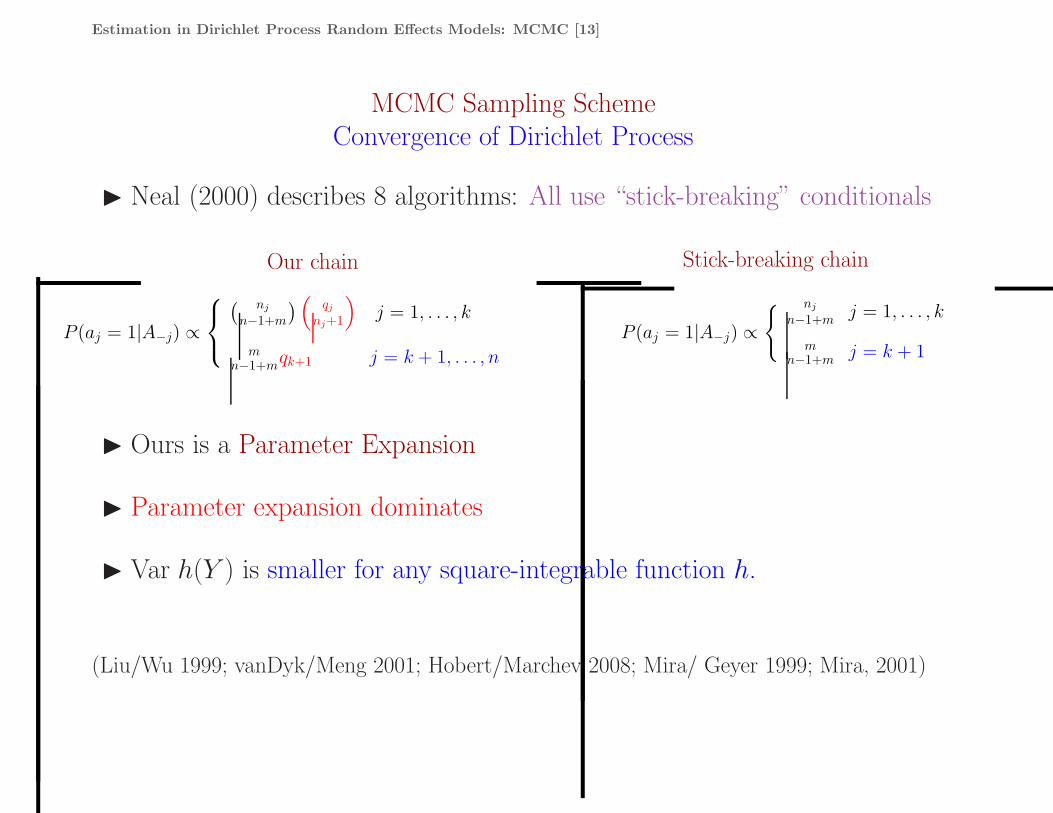
◮ Neal (2000) describes 8 algorithms: All use “stick-breaking” conditionals

Our chain Stick-breaking chain

P (aj = 1|A−j) ∝

( nj

n−1+m

) (qj

nj+1

)j = 1, . . . , k

mn−1+m

qk+1 j = k + 1, . . . , n

P (aj = 1|A−j) ∝

{ nj

n−1+mj = 1, . . . , k

mn−1+m

j = k + 1

◮ Ours is a Parameter Expansion

◮ Parameter expansion dominates

◮ Var h(Y ) is smaller for any square-integrable function h.

(Liu/Wu 1999; vanDyk/Meng 2001; Hobert/Marchev 2008; Mira/ Geyer 1999; Mira, 2001)

Estimation in Dirichlet Process Random Effects Models: Scottish Election Data [14]

Scottish Election Data - History

1997: Scottish voters overwhelmingly(74.3%) approved the creation ofthe first Scottish parliament

Our Interest:

◮ Who subsequently votedconservative in Scotland?

The voters gave strong support,(63.5%), to granting this parliamenttaxation powers

The Data:

◮ British General ElectionStudy of 880 Scottish na-tionals

◮ Outcome: party choice(conservative or not) in UKgeneral election

◮ Independent variables: po-litical and social measures

◮ Probit model


Scottish Election Data - Dirichlet Process Credible Intervals

−3 −2 −1 0 1

Politics

ReadPap

PtyThink

IDString

TaxLess

DeathPen

Lords

ScengBen

ScoPref1

RSex

Rage

RSocCla2

Tenure1

PresB

IndPar

90% Intervals for CoefficientsProbability of Voting

Conservative ↑ with:

⊲ Interest in politics(Politics)

⊲ Read newspapers(ReadPap)

⊲ Supports fewer taxes(TaxLess)

⊲ Return death penalty(DeathPen)

◮ Some Other SurprisingResults .....


Scottish Election Data - Credible Interval Comparison

−4 −3 −2 −1 0 1 2

Politics

ReadPap

PtyThink

IDString

TaxLess

DeathPen

Lords

ScengBen

ScoPref1

RSex

Rage

RSocCla2

Tenure1

PresB

IndPar

90% Intervals for Coefficients

Dirichlet= Black, Normal = Blue

Dirichlet Processvs.NormalRandomEffects

Dirichlet ProcessIntervalsUniformlyShorter

Estimation in Dirichlet Process Random Effects Models: Variance Theory [17]

Investigating the IntervalsWhy are they shorter?

Kyung, et al. (2009)Stat. and Prob. Letters

◮ Simpler Model

◮ Posterior Variance Domination

◮ Linear Mixed Model

Yij = µ + ψi + εij,

◮ Where ψ = Aη,

Y|µ,η, σ2,A ∼ N(µ1 + Aη, σ2I

)η|σ2 ∼ Nk

(0, cσ2Ik

)

µ|σ2 ∼ N(0, vσ2

)σ2 ∼ IG (a, b) ,

⊲ and the hyperparameters are assumed known.

Estimation in Dirichlet Process Random Effects Models: Variance Theory [18]

Investigating the IntervalsWhy are they shorter?

◮ Marginal posterior variance distribution π(σ2|Y,A

)

◮ We can show that

The mean from theDirichlet Process model

issmallerthan

The mean from thenormal model

⊲ For all y not containing a within-subcluster contrast

◮ Implications

⊲ The set of y containing a within-subcluster contrast has measure zero

⊲ So the dominance occurs almost surely.

Estimation in Dirichlet Process Random Effects Models: Gauss-Markov Theorem [19]

And Now for Something Completely DifferentGauss-Markov Theorem

◮ Start with the Classic Linear Mixed Model

Y = Xβ + Zψ + ε

⊲ ψ ∼ DP(m,N(0, τ 2)) ⊲ ε ∼ N(0, σ2I)

◮ Conditional on A, ψ = Aη, η ∼ N(0, τ 2I), and

Y = Xβ + ZAη + ε

◮ With Mean EY = E[E(Y |A)] = Xβ

◮ And Variance

V = Var(Y ) = E[Var(Y |A)] + Var[E(Y |A)] = E[Var(Y |A)]

Estimation in Dirichlet Process Random Effects Models: Gauss-Markov Theorem [20]

Gauss-Markov TheoremFirst Application

◮ Straightforward Application of theorem

⊲ Zyskind and Martin (1969); Harville (1976)

◮ BLUEβ = (X′V−1X)−1X′V−1Y

◮ BLUPψ = CV−1(Y − Xβ),

⊲ C = Cov(Y,ψ)

⊲ V = Var(Y )

◮ Neat Theory

⊲ What is C?

⊲ What is V?

Estimation in Dirichlet Process Random Effects Models: Covariance Matrix [21]

Using the Gauss-Markov TheoremCalculating the Variance

◮ V = Var(Y ) = E[Var(Y |A)], where

V = σ2In + E[τ 2ZAA′Z ′] = σ2In + τ 2∑

A

P (A)ZAA′Z ′.

⊲ with

P (A) = π(r1, r2, ..., rk) =Γ(m)

Γ(m + r)mk

k∏

j=1

Γ(rj).

⊲ r1, r2, ..., rk are the column sums

◮ The sum is over all possible A matrices

⊲ Lots of terms in the sum

⊲ But we can do it (almost - in a special case)


Calculating the VarianceA Special Case

◮ We can handle the model

Yij = x′iβ + ψi + εij, 1 ≤ i ≤ r, 1 ≤ j ≤ t,

⊲ which is the previous model with Z = B where

B =

1t 0 · · · 00 1t · · · 0

. . .0 0 · · · 1t

n×r

,

◮ Resulting in

d = Cor(Yi,j, Yi′,j′) = τ 2∑

A

P (A)a′iaj


Covariance MatrixA Special Case

◮ For the modelY = Xβ +Bψ + ε

◮ The covariance matrix is

V =

σ2I + τ 2J dJ dJ · · · dJ

dJ σ2I + τ 2J dJ · · · dJ... ... ... ... ...dJ dJ · · · dJ σ2I + τ 2J

,

where I is the t× t identity matrix, J is a t× t matrix of ones,

◮ And

d = Cor(Yi,j, Yi′,j′) = τ 2r−1∑

i=1

imΓ(m + r − 1 − i)Γ(i)

Γ(m + r).


Examining the CovarianceDirichlet Precision Parameter

Corr.

m

◮ Precision parameter mrelated to correlation in theobservations

◮ Relationship not previously known

◮ m ↓ yields more clusters

⊲ Decreased correlation

◮ m ↑ yields fewer clusters

⊲ Increased correlation

Estimation in Dirichlet Process Random Effects Models: OLS=BLUE [25]

AlternativelyOLS - Least Squares


◮ The OLS Estimator of β is

β = (X ′X)−1X ′Y

◮ When is OLS=BLUE?

⊲ This is “Fun with Matrix Algebra”

⊲ Relationship between X , B, and V

⊲ Zyskind (1967); Puntanen and Styan (1989)

HV = VH where H = X(X′X)−X′.

⊲ Alternative eigenvector/eigenvalue conditions

Estimation in Dirichlet Process Random Effects Models: OLS=BLUE [26]

OLS=BLUESome Conditions


◮ OLS=BLUE for

⊲ Balanced anova models

⊲ Some slight extensions

◮ In particular, for the oneway random effects model

Y = 1µ + Bψ + ε,

we have

β = (X′X)−1X′Y = (X′V−1X)−1X′V−1Y = Y.

Estimation in Dirichlet Process Random Effects Models: Distribution of Y [27]

Distribution of the BLUE Y

Oneway Model

◮ Here we look atY = 1µ + Bψ + ε,

⊲ Some results generalize (in paper)

◮ The BLUE Y has density

fm(y) =∑

A

f(y|A)P (A)

⊲ f(y|A) = N(1µ, σ2I + τ2

σ2BAA′B′)

⊲ P (A) = π(r1, r2, ..., rk) = Γ(m)Γ(m+r)

mk∏k

j=1 Γ(rj).

⊲ m is the precision parameter


Properties of fm(y)Oneway Model

◮ Unimodal

◮ m→ 0, Y ∼ N(µ, 1nσ2 + τ 2))

⊲ One Cluster

◮ m→ ∞, Y ∼ N(µ, 1n(σ2 + τ 2t))

⊲ n Clusters

⊲ Classical oneway model

◮ F0(y)︸︷︷︸Fattest Tails

< Fm(y) < F∞(y)︸︷︷︸Thinnest Tails


Distribution of the BLUE Y

Example Cutoff Points

◮ 95% Confidence Bounds

◮ Yij = µ + ψi + εij, 1 ≤ i ≤ 6, 1 ≤ j ≤ 6, , σ2 = τ 2 = 1

m

0 .1 .5 1 2 5 20 ∞

1.987 1.917 1.706 1.566 1.355 1.145 0.952 0.864

◮ Conservative Confidence Bounds

◮ Can also estimate σ2 and τ 2

Estimation in Dirichlet Process Random Effects Models: Conclusions [30]

ConclusionsModelling the Random Effects

Why is theDirichlet Processa better modelfor random effects?

◮ “Noninformative”

◮ Richer model for random effects

⊲ Normality is unverifiable

⊲ Dirichlet captures extra variation

◮ Shorter Credible Intervals

⊲ More precise inference for fixed effects


ConclusionsEstimation and MCMC

Improvements to theestimation procedureand the MCMC

◮ Matrix representation

⊲ Allows simplification

◮ Better precision parameter estimation

◮ Improved Gibbs sampler

⊲ Exploits properties of multinomial

⊲ Better mixing

⊲ Better Monte Carlo variances

Beyond theLinear Model

◮ Logistic, Loglinear

⊲ Can use Dirichlet error model

⊲ Retains estimation properties


ConclusionsClassical Approach

Point Estimation

◮ Covariance Matrix

⊲ Calculable

⊲ Interpretation of precision parameter

◮ Estimates

⊲ OLS and BLUE reasonable

Confidence Intervals

◮ Next

⊲ Variance Comparisons?

⊲ Coverage of Bayes Intervals?


Thank You for Your Attention

[email protected]


Findings So Far

◮ Gill and Casella(2009). “Nonparametric Priors For Ordinal Bayesian Social Science

Models: Specification and Estimation.” JASA, 104, 453-464

DPP on RE can uncover latent clustering.

◮ Kyung et al. (2009) “Characterizing the Variance Improvement in Linear Dirichlet Ran-

dom Effects Models.” Stat. Prob. Letters, 79, 2343-2350

DPP on RE can produce lower SE for regression parameters on average.

◮ Kyung, Gill and Casella(2010) “Estimation in Dirichlet Random Effects Models.”

Annals of Statistics, 38, 979-1009

Estimation of the precision parameter; improved Gibbs sampler.

◮ Kyung et al. (2011) “Sampling Schemes for Generalized Linear Dirichlet Process Ran-

dom Effects Models.” Stat. Methods & Applications, to appear.

Slice sampling worse than KS mixture representation or MH algorithm.

◮ Kyung et al. (2011) “New Findings from Terrorism Data: Dirichlet Process Random

Effects Models for Latent Groups.” JRSSC, to appear.

Logistic model, uncovering latent information with difficult data.

◮ Li, Chen (2011). “Classical Estimation in Linear Mixed Models with Dirichlet Process

Random Effects”. PhD Thesis, University of Florida

OLS, BLUE, and comparisons with Bayes estimates

estimation in mixed models with dirichlet process …jrojo/4th-lehmann/slides/casella.pdfestimation...

Documents