Digital Image Processing Lecture 20: Representation

& Description

Prof. Charlene TsaiProf. Charlene Tsai

* Materials from Gonzales chapter 11

2

Representation

After segmentation, we get pixels along the boundary or pixels contained in a region.

Representing a region involves two choices: Using external characteristics, e.g. boundary Using internal characteristics, e.g. color and

texture

3

Common Representation

Common external representation methods are: Chain code Polygonal approximation Signature Boundary segments Skeleton (medial axis)

We’ll discuss the first 3.

4

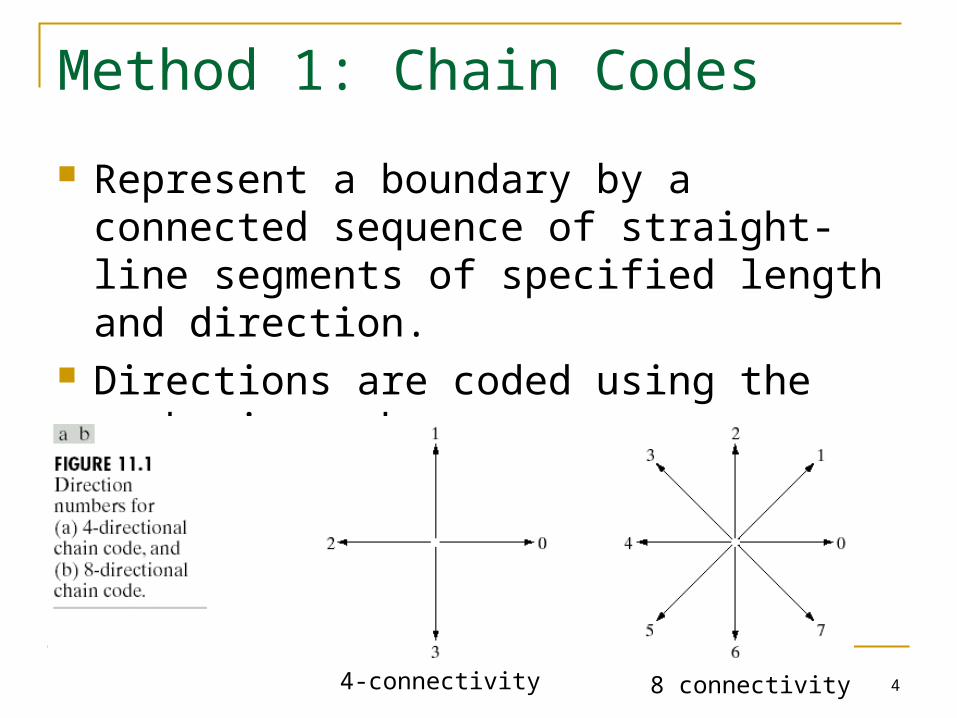
Method 1: Chain Codes

Represent a boundary by a connected sequence of straight-line segments of specified length and direction.

Directions are coded using the numbering scheme

4-connectivity 8 connectivity

5

Generation of Chain Codes

Walking along the boundary in clockwise direction, for every pair of pixels assign the direction.

Problems: Long chain Sensitive to noise

Remedies? Resampling using larger

grid spacing.

6

Resampling for Chain Codes

0033…010766…12

Spacing of the sampling grid affect the accuracy of the representation

(4-directional)(8-directional)

7

Normalization for Chain Codes With respect to starting point:

Make the chain code a circular sequence Redefine the starting point which gives an integer of

minimum magnitude E.g. 101003333222 normalized to 003333222101

For rotation: Using first difference (FD) obtained by counting the number

of direction changes in counterclockwise direction E.g FD of a 4-direction chain code 10103322 is 3133030

For scaling: Altering the size of the resampling grid.

8

Method 2: Polygonal Approximation Approximate a digital boundary with arbitrary

accuracy by a polygon. Goal: to capture the “essence” of the

boundary shape with the fewest possible polygonal segments.

9

Minimum Perimeter Polygons

Two techniques: merging & splitting

10

Merging Technique

Repeat the following steps: Merging unprocessed points along the boundary

until the least-square error line fit exceed the threshold.

Store the parameters of the line Reset the LS error to 0

Intersections of adjacent line segments form vertices of the polygon.

Problem: vertices of the polygon do not always correspond to inflections (e.g. corners) in the original boundary.

11

Splitting Technique

Subdivide a segment successively into two parts until a specified criterion is met.

For example

12

Method 3: Signature

Reduce the boundary representation to a 1D function

For example, distance vs. angle

13

(con’d)

For the signature just described Invariant to translation (everything w.r.t. the

centroid) Depending on rotation and scaling How to remove the dependence on rotation?

Selecting point farthest from the centroid Farthest point on the eigen axis (more robust) Using the chain code

How to remove the dependence on scaling? Scale all functions to span the range, say, [0,1] (not very

robust) Normalize by the variance

14

Descriptors

Boundary information can be used directly, or converted into features that describe properties of a region, such as Length of the boundary Orientation of straight line joining its extreme

points Number of concavities in the boundary

15

Boundary Descriptors (Properties) Length: approximated by the # of pixels Diameter:

Basic rectangle: defined by Major axis: the line giving the diameter Minor axis: the line perpendicular to major axis

Eccentricity: ratio of the 2 axes

jiji

ppD ,max,

16

Fourier Descriptor

Given a set of boundary points (x0, y0), (x1, y1), (x2, y2), …,. (xK-1, yK-1).

Represent the sequence of coordinates as s(k)=[xk, yk], for k=0, 1, 2, …, K-1.

Using complex representation for each point:

s(k) = xk + jyk

Advantage: reducing 2D to 1D problem

17

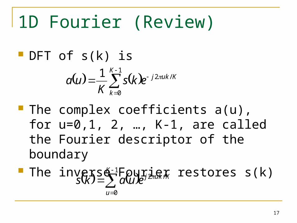
1D Fourier (Review)

DFT of s(k) is

The complex coefficients a(u), for u=0,1, 2, …, K-1, are called the Fourier descriptor of the boundary

The inverse Fourier restores s(k)

1

0

/21 K

k

KukjeksK

ua

1

0

/2K

u

Kukjeuaks

18

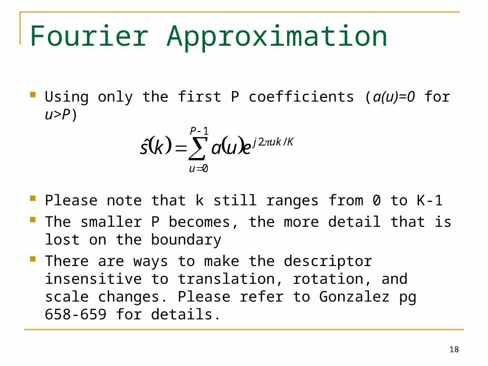
Fourier Approximation

Using only the first P coefficients (a(u)=0 for u>P)

Please note that k still ranges from 0 to K-1 The smaller P becomes, the more detail that is lost

on the boundary There are ways to make the descriptor insensitive to

translation, rotation, and scale changes. Please refer to Gonzalez pg 658-659 for details.

1

0

/2ˆP

u

Kukjeuaks

19

Example

20

Region Descriptors

Simple descriptors: Area: # of pixels in the region Perimeter: length of its boundary Compactness: (perimeter)2/area

Q: What shape gives the minimal compactness Mean and median of the gray levels.

Topological descriptors: # of holes # of connected components

21

Summary

Common external representation methods are: Chain code Polygonal approximation Signature

Descriptors Boundary descriptor Fourier descriptor Region descriptor