determining h with bayesian hyper-parameters find that part of the r11 data is down-weighted ... x...
TRANSCRIPT
Prepared for submission to JCAP
Determining H0 with Bayesianhyper-parameters
Wilmar Cardonaa Martin Kunza Valeria Pettorinob
aDépartement de Physique Théorique and Center for Astroparticle Physics, Université deGenève, 24 Quai Ernest Ansermet, 1211 Genève 4, SwitzerlandbInstitut für Theoretische Physik, Universität Heidelberg, Philosophenweg 16, D-69120 Heidel-berg, Germany
E-mail: [email protected], [email protected],[email protected]
Abstract. We re-analyse recent Cepheid data to estimate the Hubble parameter H0 byusing Bayesian hyper-parameters (HPs). We consider the two data sets from Riess et al2011 and 2016 (labelled R11 and R16, with R11 containing less than half the data of R16)and include the available anchor distances (megamaser system NGC4258, detached eclipsingbinary distances to LMC and M31, and MW Cepheids with parallaxes), use a weak metallicityprior and no period cut for Cepheids. We find that part of the R11 data is down-weightedby the HPs but that R16 is mostly consistent with expectations for a Gaussian distribution,meaning that there is no need to down-weight the R16 data set. For R16, we find a value ofH0 = 73.75 ± 2.11 km s−1 Mpc−1 if we use HPs for all data points (including Cepheid stars,supernovae type Ia, and the available anchor distances), which is about 2.6 σ larger than thePlanck 2015 value ofH0 = 67.81±0.92 km s−1 Mpc−1 and about 3.1 σ larger than the updatedPlanck 2016 value 66.93± 0.62 km s−1 Mpc−1. If we perfom a standard χ2 analysis as in R16,we find H0 = 73.46 ± 1.40 (stat) km s−1 Mpc−1. We test the effect of different assumptions,and find that the choice of anchor distances affects the final value significantly. If we excludethe Milky Way from the anchors, then the value of H0 decreases. We find however no evidentreason to exclude the MW data. The HP method used here avoids subjective rejection criteriafor outliers and offers a way to test datasets for unknown systematics.
arX
iv:1
611.
0608
8v2
[as
tro-
ph.C
O]
29
Mar
201
7

Contents
1 Introduction 1
2 Methodology 32.1 Distances and standard candles 32.2 Hyper-parameters 5
3 Expansion rate: applying hyper-parameters to R11 data 9
4 Testing assumptions 174.1 Consistency tests for Cepheid distances, using hyper-parameters 17
4.1.1 The LMC Cepheid variables 174.1.2 The Milky Way Cepheid variables 194.1.3 Cepheid variables in the megamaser system NGC 4258 224.1.4 Summarizing results 23
4.2 Metallicity dependence in the period-luminosity relation 234.3 Period cut 244.4 Hyper-parameters ensemble 254.5 Anchors 25
4.5.1 Megamaser system NGC 4258 distance modulus 254.5.2 LMC distance modulus 284.5.3 Parallax measurements of Cepheid variables in the Milky Way 284.5.4 Combining two distance anchors 294.5.5 Combining all distance anchors 304.5.6 Distance anchor summary 30
5 Final Results: applying hyper-parameters to R16 data 30
6 Discussion and Conclusions 34
A H0 and overall table of results 39
1 Introduction
Pinning down the Hubble constant H0 is crucial for the understanding of the standard modelof cosmology. It sets the scale for all cosmological times and distances and it allows to tacklecosmological parameters, breaking degeneracies among them (e.g., the equation of state fordark energy and the mass of neutrinos). The expansion rate of the universe can either bedirectly measured or inferred for a given cosmological model through cosmological probes suchas the cosmic microwave background (CMB). Although accurate direct measurements of theHubble constant have proven to be difficult (e.g., control of systematic errors, relatively smalldata sets, consistency of different methods for measuring distances), significant progress hasbeen achieved over the past decades [1, 2]. The Hubble Space Telescope (HST) Key Projectenabled a measurement of H0 with an accuracy of 10% by significantly improving the controlof systematic errors [3]. More recently, in the HST Cycle 15, the Supernovae and H0 for
– 1 –
the Equation of State (SHOES) project has reported measurements of H0 accurate to 4.7%(74.2 ± 3.6 km s−1 Mpc−1) [4], then to 3.3% (73.8 ± 2.4 km s−1 Mpc−1) [5] (called the ‘R11’data set hereafter) and very recently to 2.4% (73.24 ± 1.74 km s−1 Mpc−1) [6] (denoted as‘R16’ in the following). This remarkable progress has been achieved thanks to an improvedand expanded SN Ia Hubble diagram, including an enlarged sample of SN Ia host galaxieswith Cepheid calibrated distances, a reduction in the systematic uncertainty of the maserdistance to NGC4258, and an increase of infrared observations of Cepheid variables in theLarge Magellanic Cloud (LMC). Results were consistent with the WMAP data [7].
The 2015 release in temperature, polarization and lensing measurements of the CMB bythe Planck satellite leads to a present expansion rate of the universe given by H0 = 67.81±0.92 km s−1 Mpc−1 for the base six-parameter ΛCDM model [8]. The Planck collaborationhas recently updated this value to be H0 = 66.93 ± 0.62 km s−1 Mpc−1 [9]. The derivedestimation of H0 from CMB experiments provide indirect and highly model-dependent valuesof the current expansion rate of the universe (requiring e.g., assumptions about the natureof dark energy, properties of neutrinos, theory of gravity) and therefore do not substitute adirect measurement in the local universe. Moreover, indirect determinations (in a Bayesianapproach) rely on prior probability distributions for the cosmological parameters which mighthave an impact on the results.
The Planck Collaboration used a “conservative” prior on the Hubble constant (H0 =70.6 ± 3.3 km s−1 Mpc−1) derived from a reanalysis of the Cepheid data used in [5], doneby G. Efstathiou in [10]: in this reanalysis, a different rejection algorithm was used (withrespect to that in [5]) for outliers in the Cepheid period-luminosity relation (the so-calledLeavitt Law); in addition, [10] used the revised geometric maser distance to NGC4258 of [11].Although consistent with the Planck TT estimate at the 1σ level, this determination of H0
assumes that there is no metallicity dependence in the Leavitt Law. Furthermore, it discardsdata (i) from both Large Magellanic Cloud (LMC) and Milky Way (MW) Cepheid variables(ii) from the sample of Cepheid variables in [5] using an upper period cut of 60 days.1
As discussed in [2], the sensitivity to metallicity of the Leavitt Law is still an open ques-tion. In fact, due to changes in the atmospheric metal abundance, a metallicity dependencein the Cepheid period-luminosity is expected. Discarding data involves somehow arbitrarychoices (e.g., Chauvenet’s criterion, period cut, threshold T in [10]) and might hinder ourunderstanding of the physical basis behind the incompatibility of data sets (if any) [12].Therefore, neither no metallicity dependence in Leavitt Law nor disregarding data seem tobe a priori very conservative assumptions.
Once systematics are under control (like the presence of unmodeled systematic errors orbiases in the outlier rejection algorithm for Cepheid variables), a reliable estimate ofH0 is veryimportant also on theoretical grounds. Confirmation of significant discrepancies between dir-ect and indirect estimates of H0 would suggest evidence of new physics. Discrepancies couldarise if the local gravitational potential at the position of the observer is not consistentlytaken into account when measuring the Hubble constant. Nevertheless, an unlikely fluctu-ation would be required as estimates of ∆H0 from inhomogeneities are of the order of 1 – 2
1In [10] G. Efstathiou also shows results utilizing the rejection algorithm for outliers used in [5], but withthe revised geometric maser distance to NGC4258 [11] which is about 4% higher than that adopted by [5] intheir analysis. Note that in [5] (see their page 13) the authors provided a recalibration of H0 for each increaseof 1% in the distance to NGC4258: according to this recalibration and the revised geometric maser distancetheir measurement would be driven downwards from H0 = 74.8 km s−1 Mpc−1 to H0 ≈ 73.8 km s−1 Mpc−1
which is higher than all the reported values in table A1 of [10] for the R11 rejection algorithm.
– 2 –

km s−1 Mpc−1 only [13, 14], although there are claims that observations support the existenceof a sufficiently large local departure from homogeneity [15]. Second-order corrections to thebackground distance-redshift relation could bias estimations of the Hubble constant derivedfrom CMB [16]. However, it was shown in [17] that those corrections are already taken intoaccount in current CMB analyses.
It is clear from [10] that the statistical analysis done when measuring H0 plays a partin the final result (for instance, through the outlier rejection algorithm, data sets included,anchors distances included, the period cut on the sample of Cepheid variables, the prior on theparameters of the Period-Luminosity relation). Given the relevance of the Hubble constantfor our understanding of the universe, it is necessary to confirm previous results and provethem robust against different statistical approaches.
The goal of this paper is to determine the Hubble constant H0 by using Bayesian hyper-parameters in the analysis of the Cepheid data sets used in both [5] and [6]. In Section 2 weexplain both our notation and the statistical method employed. We then apply the methodto the R11 data set and determine the expansion rate H0 in Section 3. In Section 4 we testthe assumptions of our baseline analysis. The reader willing to know our main results usingthe R16 data set can skip Section 3 and 4 and go directly to Section 5. We conclude anddiscuss our results in Section 6.
2 Methodology
2.1 Distances and standard candles
Astrophysical objects with a known luminosity – the so-called standard candles – are usedto probe the expansion rate of the universe. In particular, measuring redshifts and apparentluminosities for supernovae type Ia (SNe Ia) one can establish an empirical redshift-distancerelation for these objects. In order to estimate distances to SNe Ia one uses the luminositydistance
dL ≡(L
4πl
)1/2
, (2.1)
where L and l are the absolute luminosity and the apparent luminosity, respectively. Forhistorical reasons the apparent bolometric luminosity l is defined so that
l = 10−2m/5 × 2.52× 10−5 erg/cm2 s (2.2)
where m is the apparent bolometric magnitude [18]. Similarly, one can define the absolutebolometric magnitude M as the apparent bolometric magnitude a source would have at adistance 10 pc
L = 10−2M/5 × 3.02× 1035 erg/s. (2.3)
Combining equations (2.1)–(2.3) it is possible to express the luminosity distance in terms ofthe distance modulus m−M :
µ0 ≡ m−M = 5 log10
(dL
1Mpc
)+ 25 . (2.4)
One can also compute the luminosity distance dL of a light source with redshift z in thecontext of General Relativity. Assuming a flat FLRW metric, one finds
dL(z) = (1 + z)c
∫ z
0
dz′
H(z′)(2.5)
– 3 –
where c is the speed of light and H(z) is the Hubble function. Since nowadays the empiricalcurve for dL(z) is reasonably well known for relatively small redshift, the Hubble functionmay then be usefully expressed as a power series in Eq. (2.5), leading to
dL(z) ≡ cz
H0(1 + δ(z)) ≈ cz
H0
{1 +
1
2[1− q0]z − 1
6[1− q0 − 3q2
0 + j0]z2 +O(z3)
}(2.6)
where H0 is the Hubble constant, q0 is the present acceleration parameter, j0 the present thepresent jerk parameter. Here δ(z) defines a function that vanishes as z → 0 and that for smallredshifts, z � 1, can be approximately expressed as a series expansion in redshift startingwith a term linear in z. Using an expansion instead of Eq. (2.5) with the ΛCDM expressionfor H(z) has the advantage that it is more model independent.
We now have dL as a function of m and M in (2.4) and an expression of dL in terms ofthe expansion rate today (2.6). Equating Eqs. (2.4) and (2.6) we obtain that
5 log10(cz(1 + δ(z)))−mX = 5 log10H0 −MX − 25 ≡ 5aX , (2.7)
where X denotes the use of wavelength band X (e.g., U for ultraviolet, B for blue, and Vfor visual) and aX is a constant which defines the intercept of the log10 cz − 0.2mX relation.Defining δ(z) through q0 = −0.55 and j0 = 1 [19], Riess et al. [5] used the V wavelengthband Hubble diagram for 153 nearby SN-Ia in the redshift range 0.023 < z < 0.1 2 to measurethe intercept aV = 0.697± 0.00201. Using the Hubble diagram for 217 SNe Ia in the redshiftrange 0.023 < z < 0.15, Riess et al. [6] found aB = 0.71273± 0.00176.
From Eqs. (2.4) and (2.7) one can easily express the apparent magnitude mSNe IaX of a
SN Ia in terms of its distance modulus µ0, the Hubble constant H0, and the intercept aX as
mSNe IaX = 5 log10H0 + µ0 − 5aX − 25 . (2.8)
Having measured aX we can find H0 if we know µ0 for a supernova for which have measuredmSNe IaX . Unfortunately, we generally do not have a direct measurement of µ0 for objects that
contain supernovae. In this situation Cepheid variables – another type of standard candles –come to the rescue. Cepheids are stars whose apparent luminosity is observed to vary more orless regularly with time. They are quite common, so that there exist several galaxies (19 up todate [6]) which simultaneously host both SNe Ia and Cepheid variables, and in addition severalgalaxies for which we have measured the distance directly so that µ0 is known and which alsohost Cepheids. This is the case for the megamaser system NGC4258, LMC, M31 as well asfor individual Cepheids in the Milky Way. Although the sample of MW Cepheid variableswith parallax measurements is relatively small (15 up to date [6]) and mostly dominated byCepheid stars with periods P < 10 days, their inclusion helps to further constrain parametersin the period-luminosity relation.
The apparent luminosity of Cepheids and its link to µ0 is described by the Leavitt Law[20]. According to the Leavitt Law there is a relation between period and luminosity ofCepheids: in the ith galaxy, the pulsation equation for the jth Cepheid star with apparentmagnitude mCepheid
Y,i,j (in the passband Y , not necessarily the same as passband X for thesupernovae) and period Pi,j leads to a relation
mCepheidY,i,j = µ0,i +MCepheid
Y + bY (logPi,j − 1) + ZY ∆ log[O/H]i,j , (2.9)
2A conservative lower limit in redshift imposed to avoid the possibility of a local, coherent flow biasing theresults.
– 4 –
where ZY is the metallicity parameter, bY is the slope of the period-luminosity relation, andMCepheidY is the Cepheid zero point which is common to all Cepheids. A fit of Eq. (2.9) for
the galaxies with known µ0 that host Cepheids allows us to determine the parameters bY ,ZY and especially MCepheid
Y which is fully degenerate with µ0,i. Using then the Leavitt lawwith now known MCepheid
Y for the galaxies with Cepheids and supernovae allows to determinethe µ0 of those galaxies, effectively transferring the distance measurements from the ‘anchors’(with direct distance determinations) to the ‘supernova hosts’. Knowing µ0 for the supernovahosts we can finally use Eq. (2.8) to determine H0. In reality of course we will fit everythingsimultaneously.
2.2 Hyper-parameters
Astrophysical observations are difficult, and it is not easy to estimate and include the asso-ciated errors and uncertainties correctly. Often the data sets show outliers with error barsthat are much smaller than the deviation from the expected fit, for reasons that are not wellunderstood or difficult to quantify. An analysis needs to deal with such outliers, typically byremoving them based on some rejection rule. As discussed in [4, 5, 10], the rejection of outlierson the Cepheid period-luminosity relation may have a non-negligible effect on the determin-ation of the expansion rate of the universe. One can argue that an outlier rejection criterion:i) involves arbitrary choices (e.g., Chauvenet’s criterion, period cut) which might bias theresults; ii) rejects data, thus increasing error bars and hindering a better understanding ofthe data sets [12]. The hyper-parameter (HP, hereafter) method offers a Bayesian alternativeto ad hoc selection of data points, avoiding problems associated with using incompatible datapoints [21, 22]. Instead of adopting an a priori rejection criterion (galaxy-by-galaxy as in[4, 5] or from a global fit as in [6, 10]), in this work we analyse all the available measurementswith Bayesian HPs. The latter effectively allow for relative weights in the Cepheid variables,determined on the basis of how good their simultaneous fit to the model is.
HPs allow to check for unrecognised systematic effects by introducing a rescaling of theerror bar of data point i, σi → σi/
√αi. Here αi is a HP associated with the data point i
[21, 22]. In order to explain how HPs work, we start by assuming a Gaussian likelihood forthe datum Di,
PG(Di|~w) = Niexp(−χ2
i (~w)/2)√2π
, (2.10)
where χ2i and the normalisation constant Ni are given by
χ2i ≡
(xobs,i − xpred,i(~w))2
σ2i
, Ni = 1/√σ2i . (2.11)
Here for each measurement xobs,i there is a corresponding error σi and a prediction xpred,i(~w),(~w being the parameters of a given model). Suppose that some errors have been wrongly es-timated due to unrecognised (or underestimated) systematic effects and use hyper-parameters[21] to control the relative weight of the data points in the likelihood. For each measurementi we introduce a HP to rescale σi as mentioned above. In that case the Gaussian likelihoodbecomes [21]
P (Di|~w, αi) = Ni α1/2i
exp(−αiχ2i (~w)/2)√
2π. (2.12)
However, in general we do not know what value of αi is correct. In order to circumventthis problem, we follow a Bayesian approach, introducing the αi as nuisance parameters and
– 5 –
marginalising over them. Given a set of data points {Di}, we can write the probability forthe parameters ~w as
P (~w|{Di}) =
∫· · ·∫P (~w, {αi}|{Di}) dα1 . . . dαN , (2.13)
where N is the total number of measurements. Bayes’ theorem allows us to write
P (~w, {αi}|{Di}) =P ({Di}|~w, {αi})P (~w, {αi})
P (D1, . . . , DN )(2.14)
andP (~w, {αi}) = P (~w|{αi})P ({αi}). (2.15)
As in [21] we assume:
P ({Di}|~w, {αi}) = P (D1|~w, α1) . . . P (DN |~w, αN ), (2.16a)P (~w|{αi}) = constant, (2.16b)P ({αi}) = P (α1) . . . P (αN ). (2.16c)
Combining Eqs. (2.14)–(2.16a) the integrand in Eq. (2.13) then reads:
P (~w, {αi}|{Di}) =P (D1|~w, α1) . . . P (DN |~w, αN )P (~w|{αi})P ({αi})
P (D1, . . . , DN )(2.17)
=P (D1|~w, α1) . . . P (DN |~w, αN )P (~w|{αi})P (α1) . . . P (αN )
P (D1, . . . , DN ). (2.18)
Thus far the formalism is fairly general and it contains two unspecified functions: theprobability distributions for HPs and data points. In this work we will assume uniform priorsfor HPs (P (αi) = 1) and that errors are never actually smaller than the value given (i.e.error bars tend to be underestimated, not overestimated, leading to αi ∈ [0, 1]).3 A lowposterior value of the HP indicates that the point has less weight within the fit. This mayindicate the presence of systematic effects or the requirement for better modelling. Withthese assumptions the integrand in Eq.(2.13) becomes
P (~w, {αi}|{Di}) = constant× P (D1|~w, α1) . . . P (DN |~w, αN )
P (D1, . . . , DN )(2.19)
and Eq. (2.13) now reads
P (~w, {Di}) = constant× P (D1|~w) . . . P (DN |~w)
P (D1, . . . , DN ), (2.20)
where
P (Di|~w) ≡∫ 1
0P (Di|~w, αi) dαi. (2.21)
3We have examined the more general case of an improper Jeffrey’s prior (allowing decreasing as well asincreasing error bars). This works well when many data points are associated to the same HP so that the χ2
never vanishes. But when each data point has its own associated HP then the model curve can pass throughthat data point so that χ2
i = 0. In this case the likelihood grows without bounds as αi → 0, in other wordsthe HP-marginalised likelihood is singular when at least one of the points has χ2 = 0 as can also be seen fromEq. (16) in [21].
– 6 –
The integral in Eq. (2.21) can be explicitly evaluated for the Gaussian HP likelihood(2.12), and gives, for each data point,
P (Di|~w ) = Ni
Erf(χi(~w)√
2
)−√
2πχi(~w) exp(−χ2
i (~w)/2)
χ3i (~w)
≡ Niχ2i (χ
2i (~w)). (2.22)
which defines the effective χ square function χ2i . We can now rewrite Eq. (2.20) as
lnP (~w, {Di}) =∑i
ln Ni + ln χ2i , (2.23)
where constant terms have been omitted.Since we have analytically marginalized over the hyper-parameters, they no longer ap-
pear in the posterior distribution. Each HP however does have a posterior pdf associated withit, and we could determine it by adding a HP explicitly as a parameter and including it in thesampling procedure. In general this might entail adding thousands of extra parameters, whichwould make the exploration of the posterior numerically much more demanding. However,one can easily obtain the most likely value (the peak or mode of the pdf) for each HP bymaximizing (2.12) with respect to the HPs at a given set of best fit parameters ~w. We findthat for each data point the most likely value is given by
αeffi = 1, if χ2
i ≤ 1 (2.24a)
αeffi =
1
χ2i
, if χ2i > 1. (2.24b)
Although this point-estimate of the hyper-parameter posterior does not contain the full in-formation, we can nonetheless use these effective HP values to flag data points that, if down-weighted, improve the overall likelihood. We consider this a sign that they are not fullycompatible with the other data points, for the model adopted.
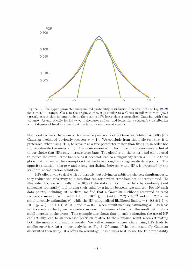
In Fig. 1 we show the hyper-parameter marginalized pdf (left hand side of Eq. (2.23))for a single datum with standard deviation σ = 1 (orange line) and compare it to a Gaussiancurve (green line) with the same curvature at the peak (corresponding to σ =
√5/3) and the
same amplitude at zero (which is about 16% lower than the amplitude of a Gaussian pdf,as the HP-marginalized has wider wings) and to a student’s t distribution with two degreesof freedom (blue line). We see that close to the peak the HP marginalised pdf looks like aGaussian, while it decays as a power law (∝ x−3) as we move away from the peak, like thestudent’s t distribution. This is not really a surprise as the student’s t distribution arises whenmarginalising a Gaussian pdf over σ, which is partially also the case for the HP-marginalisedpdf.
As the hyper-parameter marginalized likelihood (orange line) has a lower curvature atthe peak and wider tails than the original Gaussian pdf (green line in Fig. 1), we expect thatit will lead to a less precise determination of parameters for a given, fixed σ, with respectto the standard analysis which does not include hyperparameters. This is indeed the case:we find numerically that for a large ensemble of 106 data points drawn independently froma univariate Gaussian pdf, the uncertainty on the mean of the HPs posterior distributionis about 40% larger than for a Gaussian likelihood. If we however estimate the variance σthat enters Eq. (2.11) simultaneously with the mean then the hyper-parameter marginalised
– 7 –
-10 -5 0 5 10x
0.005
0.010
0.050
0.100
0.500PDF
Figure 1. The hyper-parameter marginalized probability distribution function (pdf) of Eq. (2.22)for σ = 1, in orange. Close to the origin, x = 0, it is similar to a Gaussian pdf with σ =
√5/3
(green), except that its amplitude at the peak is 16% lower than a normalised Gaussian with thatvariance. Asymptotically for |x| → ∞ it decreases as 1/x3 and looks like a student’s t distributionwith 2 degrees of freedom (blue), but the latter is narrower at small x.
likelihood recovers the mean with the same precision as the Gaussian, while σ is 0.606 (theGaussian likelihood obviously recovers σ = 1). We conclude from this little test that it ispreferable, when using HPs, to leave σ as a free parameter rather than fixing it, in order notto overestimate the uncertainty. The main reason why this procedure makes sense is linkedto our choice that HPs only increase error bars. The global σ on the other hand can be usedto reduce the overall error bar size as it does not lead to a singularity when σ → 0 due to itsglobal nature (under the assumption that we have enough non-degenerate data points). Theopposite situation, a large σ and strong correlations between σ and HPs, is prevented by thestandard normalization condition.
HPs offer a way to deal with outliers without relying on arbitrary choices; simultaneously,they reduce the sensitivity to biases that can arise when error bars are underestimated. Toillustrate this, we artificially turn 10% of the data points into outliers by randomly (andsomewhat arbitrarily) multiplying their value by a factor between two and ten. For 106 suchdata points, including 105 outliers, we find that a Gaussian likelihood (centered at zero)recovers a mean of µ = (−4.7 ± 1.0) × 10−3 (µ = (−4.7 ± 2.2) × 10−3 and σ = 2.2 whensimultaneously estimating σ), while the HP marginalised likelihood finds µ = (−0.8± 1.5)×10−3 (µ = (−0.6 ± 1.1) × 10−3 and σ = 0.70 when simultaneously estimating σ). At leastin this scenario the hyper-parameters successfully remove a bias from the result with only asmall increase in the errors. This example also shows that in such a situation the use of HPcan actually lead to an increased precision relative to the Gaussian result when estimatingboth the mean and σ simultaneously. We will encounter a case where using HPs leads tosmaller error bars later in our analysis, see Fig. 7. Of course if the data is actually Gaussiandistributed then using HPs offers no advantage, it is always best to use the true probability
– 8 –
distribution function when this is possible. The advantage of HPs comes from allowing us todeal with situations where the true pdf is uncertain.
The use of HPs when combining different data also offers a way to test for internalconsistency by checking if the average effective HP values, Eqs. (2.24a) and (2.24b), are lowerthan expected. To this end we define the normalised weight of jth kind of data as
||αj || ≡∑Kj
i=1 αi,jKj
, (2.25)
where αi,j denotes ith HP of data of kind j (j = Cepheid, SNe Ia, Anchors), and Kj standsfor the number of objects of kind j. A low normalised weight ||αj || in (2.25) for a given kindj of data is an indicator for problems e.g. in the report error bars or the data values, or in themodel used to fit the data. However, there are also points outside of the 1σ region for datadrawn from the expected Gaussian distribution, it is straightforward to compute from Eqs.(2.24) that we expect ||α|| ≈ 0.85 in this situation. Data sets with a value of ||α|| close to0.85 can be considered reliable. Smaller values indicate too many outliers relative to the givenerror bars – the numerical example with 10% of outliers mentioned above has ||α|| = 0.79. Itis also possible to use the effective HP to test whether data sets are mutually consistent. Ifthey are not, then the global fit to the combined data may reduce the normalised weights ofeach data set. We will use this later to decide on some of the choices that need to be madeto analyse the distance data.
We will now apply HPs to combine Cepheid variable measurements and determine thecurrent expansion rate of the universe. We explore the parameter space ~w with the helpof a Markov Chain Monte Carlo (MCMC) approach, using flat priors if not specified differ-ently. A summary of all the fits done for this work are illustrated in Tables 10–11, where wetested different assumptions. We will now first describe our baseline choice and the resultingconstraint on H0 and then, in Section 4, describe in detail each of the assumptions.
3 Expansion rate: applying hyper-parameters to R11 data
In this section we describe our baseline HP marginalised analysis of the local expansion ratedata. As we will discuss in more detail below, we include three different distance anchors,we use hyper-parameters everywhere (Cepheids, supernovae and anchors), we do not apply aperiod cut in the Cepheid data and use a strong prior on Cepheid metallicity. We considerthe resulting constraint on H0 corresponding to this set of ‘baseline choices’ [fit (29) in Tables10–11] as our ‘best estimate’ for the R11 data set [5]. In Section 4 we will then study whathappens if we change these assumptions.
The R11 data set It comprehends a sample of 53 Large Magellanic Cloud (LMC) Cepheidvariables with H-band magnitudes, mH , listed in Table 3 of [23] and V , I band magnitudes,mV , mI , listed in Table 4 of [24]; the sample of Cepheid variables in the 8 SNe Ia hosts of[5]; 13 Milky Way (MW) Cepheid stars with parallax measurements listed in Table 2 of [25](eliminating Polaris and correcting for Lutz-Kelker bias).
Baseline anchors We will show in Section 4.1 that the period-luminosity parameters inde-pendently derived from LMC, MW and NGC 4258 Cepheid variables are in good agreementand therefore we do not see any reason to discard any of the data sets when determining theHubble constant with hyper-parameters. Here we use the sample of Cepheid variables for the
– 9 –
SNe Ia hosts from [5], the set of LMC Cepheid variables discussed in Section 4.1.1 and theset of MW Cepheid variables discussed in Subsection 4.1.2. The MW Cepheid zero-pointshave been determined with the help of their parallax distance so that they contribute to theabsolute distance determinations. We further use both the revised NGC4258 geometric maserdistance from [11] and the distance to NGC4258 determined by considering type IIP SNe from[26]. We also make use of the distance to LMC derived from observations of eclipsing binariesfrom [27]. In Subsection 4.5 we study how our method performs for different combinations ofanchor distances.
Baseline HPs We use hyper-parameters everywhere, for Cepheids, supernovae and anchors.In particular, we use hyper-parameters for all Cepheid fits as there are outliers in most ofthe data sets. As for supernovae, we find that the SNe Ia data show potential inconsistenciesin our fits (see Figure 5 and Table 1 below), therefore we include hyper-parameters alsoin supernovae. We further include hyper-parameters in the available distance moduli toboth NGC 4258 and LMC. For anchor distances and SNe Ia magnitudes we then assume aGaussian HP likelihood as in Eq. (2.22). Hence in order to find the best-fitting parameters~w we maximize
lnP (~w, {Di}) = lnPCepheid + lnP SNe Ia + lnPAnchors. (3.1)
For Cepheid variables we have, applying Eq. (2.23),
lnPCepheid =∑ij
ln χ2(χ2,Cepheidij ) + ln NCepheid
ij , (3.2a)
where the index i identifies the galaxy and the index j refers to the Cepheid belonging to theith galaxy; here
χ2,Cepheidij =
(mW,ij −mPW,i,j)
2
σ2e,ij + σ2
int,i
, NCepheidij =
1√σ2e,ij + σ2
int,i
, (3.2b)
and the Cepheid magnitude mW,ij is modelled as in Eq. (2.9); for the ‘Wesenheit reddening-free’ magnitudes, denoted by W , that combine H, V, I bands:
mW,ij = mH,ij − 0.410 (mV,ij −mI,ij) ; (3.2c)
finally σint,i is the internal scatter for the ith galaxy. The internal scatter is a commonadditional dispersion of the data points that is independent of the measurement error anddue to variations in the physical mechanism behind the period-luminosity relation [10]. Inthe R11 data set the internal scatter is not known, it is estimated simultaneously to the otherparameters and can then be marginalized over if we are not interested in its distribution.More precisely, we sample in log σint with a flat prior lnσint ∈ [−3,−0.7]. As discussed inSection 2.2, allowing for a free σ also permits to avoid artificially inflating the uncertaintyon the inferred parameter values when using HPs. Indeed, as we will see in the next section,HPs can even allow to decrease the posterior uncertainty, as they allow to use a smaller σint
by down-weighting outliers that lead to a non-Gaussian distribution with heavier tails.For SNe Ia we use the likelihood:
lnP SNe Ia =∑i
ln χ2(χ2,SNe Iai )+ln NSNe Ia
i −(aR11V − aV )2
2σ2aV
−ln(2πσ2
aV)
2− (acal)
2
2σ2acal
−ln(2πσ2
acal)
2
(3.3a)
– 10 –
where
χ2,SNe Iai =
(m0V,i −mth
V,i)2
σ2i
, NSNe Iai =
1√σ2i
, (3.3b)
mthV,i = µ0,i + 5 logH0 − 25− 5aV , (3.3c)
andm0V,i, σi are taken from the table 3 in [5]. Here aV is the intercept of the SNe Ia magnitude-
redshift relation, and [5] gives its value as aV = 0.697 ± 0.00201. We call the mean valuein the above expression for the likelihood aR11
V = 0.697, the uncertainty σaV = 0.00201 andassume that aV itself has a Gaussian pdf given by these quantities. If we were dealing withGaussian likelihood for m0
V,i then we could marginalize analytically over aV , which wouldthen contribute a fully correlated error to the covariance matrix for the m0
V,i. But as we areusing HPs, we instead add aV as an explicit (nuisance) parameter in Eq. (3.3a), together withits associated Gaussian likelihood, and sample from it numerically. Similarly, we take intoaccount the calibration error, σacal , between the ground based and the WFC3 photometry byintroducing a nuisance parameter acal. We assume it has a Gaussian pdf with zero mean andσacal = 0.04.
Finally, motivated by the inconsistencies of distance anchors found by G. Efstathiou in[10], we include hyper-parameters also when dealing with the available distance moduli:
lnPAnchors = ln χ2
((µ0,4258 − µobs1
0,4258)2
σ2obs1,4258
)−
ln(2πσ2obs1,4258)
2
+ ln χ2
((µ0,4258 − µobs2
0,4258)2
σ2obs2,4258
)−
ln(2πσ2obs2,4258)
2
+ ln χ2
((µ0,LMC − µobs
0,LMC)2
σ20,LMC
)−
ln(2πσ20,LMC)
2(3.4)
where the numerical values for µobs0,LMC are given by Eq. (4.6) and µobs1
0,4258, µobs20,4258 in equations
(4.14) and (4.15), respectively.
Baseline Cepheid period At this point we have assembled all ingredients necessary to de-termine the Hubble parameter, using HPs rather than a rejection algorithm. A few additionalchoices are however necessary. The first one concerns the period cut for the Cepheids: [5]uses periods up to 205 days (effectively equivalent to no period cut), while [10] limits himselfto periods shorter than 60 days. As we will discuss in the next section, we see no significanttrend for the LMC and MW Cepheid stars that would justify a tighter cut when using theR11 data. For our choice of the baseline, discussed in this section, we perform no cut in theperiod (equivalent to choosing a 205 days cut as [5]); in the next section, we also perform theanalysis for both cuts and report the results in Table 5. The difference between using datawith P < 60 or P < 205 is smaller than 0.5 km s−1 Mpc−1 in H0 (with a somewhat largerimpact on bW ). For this reason we use the larger data set, P < 205, for our final numbers.
Baseline metallicity in Leavitt Law The second choice concerns the treatment of ametallicity dependence in the Cepheid fits. As we will discuss in Subsection 4.2, this is still anopen question. The combined Cepheid data used here is unable to significantly constrain ZW ,instead we find a strong degeneracy withMW (see Fig. 3). From a Bayesian model comparisonpoint of view, there is no significant preference for specific priors or ZW = 0. However, looking
– 11 –
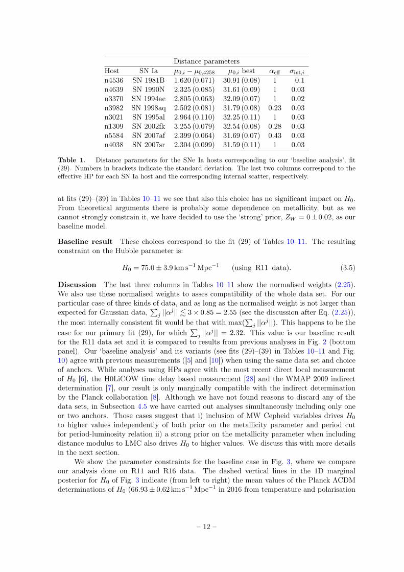
Distance parametersHost SN Ia µ0,i − µ0,4258 µ0,i best αeff σint,i
n4536 SN 1981B 1.620 (0.071) 30.91 (0.08) 1 0.1n4639 SN 1990N 2.325 (0.085) 31.61 (0.09) 1 0.03n3370 SN 1994ae 2.805 (0.063) 32.09 (0.07) 1 0.02n3982 SN 1998aq 2.502 (0.081) 31.79 (0.08) 0.23 0.03n3021 SN 1995al 2.964 (0.110) 32.25 (0.11) 1 0.03n1309 SN 2002fk 3.255 (0.079) 32.54 (0.08) 0.28 0.03n5584 SN 2007af 2.399 (0.064) 31.69 (0.07) 0.43 0.03n4038 SN 2007sr 2.304 (0.099) 31.59 (0.11) 1 0.03
Table 1. Distance parameters for the SNe Ia hosts corresponding to our ‘baseline analysis’, fit(29). Numbers in brackets indicate the standard deviation. The last two columns correspond to theeffective HP for each SN Ia host and the corresponding internal scatter, respectively.
at fits (29)–(39) in Tables 10–11 we see that also this choice has no significant impact on H0.From theoretical arguments there is probably some dependence on metallicity, but as wecannot strongly constrain it, we have decided to use the ‘strong’ prior, ZW = 0± 0.02, as ourbaseline model.
Baseline result These choices correspond to the fit (29) of Tables 10–11. The resultingconstraint on the Hubble parameter is:
H0 = 75.0± 3.9 km s−1 Mpc−1 (using R11 data). (3.5)
Discussion The last three columns in Tables 10–11 show the normalised weights (2.25).We also use these normalised weights to asses compatibility of the whole data set. For ourparticular case of three kinds of data, and as long as the normalised weight is not larger thanexpected for Gaussian data,
∑j ||αj || . 3× 0.85 = 2.55 (see the discussion after Eq. (2.25)),
the most internally consistent fit would be that with max(∑
j ||αj ||). This happens to be thecase for our primary fit (29), for which
∑j ||αj || = 2.32. This value is our baseline result
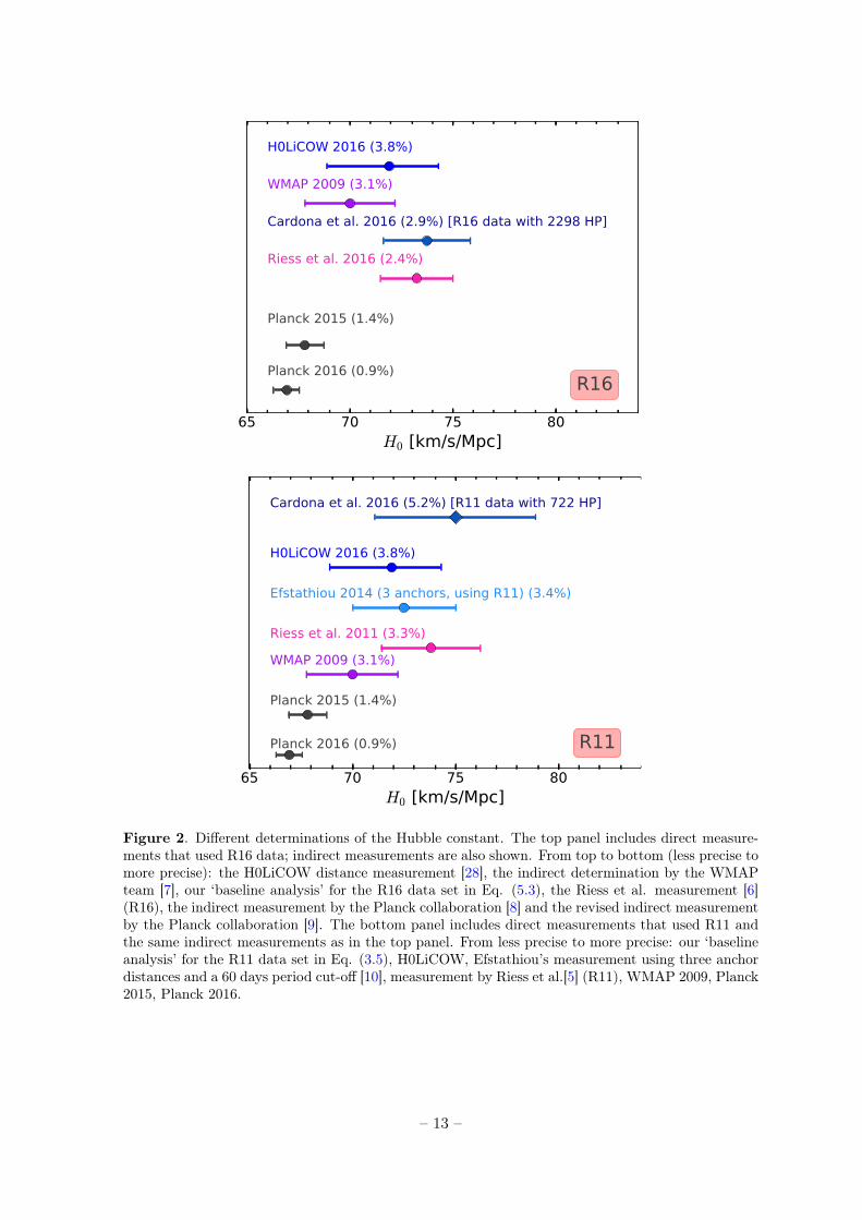
for the R11 data set and it is compared to results from previous analyses in Fig. 2 (bottompanel). Our ‘baseline analysis’ and its variants (see fits (29)–(39) in Tables 10–11 and Fig.10) agree with previous measurements ([5] and [10]) when using the same data set and choiceof anchors. While analyses using HPs agree with the most recent direct local measurementof H0 [6], the H0LiCOW time delay based measurement [28] and the WMAP 2009 indirectdetermination [7], our result is only marginally compatible with the indirect determinationby the Planck collaboration [8]. Although we have not found reasons to discard any of thedata sets, in Subsection 4.5 we have carried out analyses simultaneously including only oneor two anchors. Those cases suggest that i) inclusion of MW Cepheid variables drives H0
to higher values independently of both prior on the metallicity parameter and period cutfor period-luminosity relation ii) a strong prior on the metallicity parameter when includingdistance modulus to LMC also drives H0 to higher values. We discuss this with more detailsin the next section.
We show the parameter constraints for the baseline case in Fig. 3, where we compareour analysis done on R11 and R16 data. The dashed vertical lines in the 1D marginalposterior for H0 of Fig. 3 indicate (from left to right) the mean values of the Planck ΛCDMdeterminations of H0 (66.93± 0.62 km s−1 Mpc−1 in 2016 from temperature and polarisation
– 12 –
65 70 75 80H0 [km/s/Mpc]
R16Planck 2016 (0.9%)
Planck 2015 (1.4%)
Riess et al. 2016 (2.4%)
Cardona et al. 2016 (2.9%) [R16 data with 2298 HP]
WMAP 2009 (3.1%)
H0LiCOW 2016 (3.8%)
65 70 75 80H0 [km/s/Mpc]
R11Planck 2016 (0.9%)
Planck 2015 (1.4%)
WMAP 2009 (3.1%)
Riess et al. 2011 (3.3%)
Efstathiou 2014 (3 anchors, using R11) (3.4%)
H0LiCOW 2016 (3.8%)
Cardona et al. 2016 (5.2%) [R11 data with 722 HP]
Figure 2. Different determinations of the Hubble constant. The top panel includes direct measure-ments that used R16 data; indirect measurements are also shown. From top to bottom (less precise tomore precise): the H0LiCOW distance measurement [28], the indirect determination by the WMAPteam [7], our ‘baseline analysis’ for the R16 data set in Eq. (5.3), the Riess et al. measurement [6](R16), the indirect measurement by the Planck collaboration [8] and the revised indirect measurementby the Planck collaboration [9]. The bottom panel includes direct measurements that used R11 andthe same indirect measurements as in the top panel. From less precise to more precise: our ‘baselineanalysis’ for the R11 data set in Eq. (3.5), H0LiCOW, Efstathiou’s measurement using three anchordistances and a 60 days period cut-off [10], measurement by Riess et al.[5] (R11), WMAP 2009, Planck2015, Planck 2016.
– 13 –
65 70 75 80 85 90
H0
18.3018.3618.4218.4818.5418.60
µ0,LMC
7
6
5
4
3
Mw
0.40.30.20.10.00.10.2
Zw
3.36
3.28
3.20
3.12
3.04
b w
29.04
29.12
29.20
29.28
29.36
29.44
µ0,4258
657075808590
H0
18.30
18.36
18.42
18.48
18.54
18.60
µ0,LMC
7 6 5 4 3
Mw
0.40.3
0.20.1
0.00.1
0.2
Zw
3.363.28
3.203.12
3.04
bw
Cardona et al. 2016 (5.2%) [R11]Cardona et al. 2016 (2.9%) [R16]
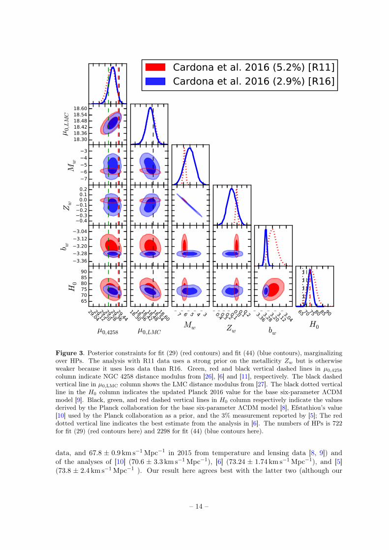
Figure 3. Posterior constraints for fit (29) (red contours) and fit (44) (blue contours), marginalizingover HPs. The analysis with R11 data uses a strong prior on the metallicity Zw but is otherwiseweaker because it uses less data than R16. Green, red and black vertical dashed lines in µ0,4258
column indicate NGC 4258 distance modulus from [26], [6] and [11], respectively. The black dashedvertical line in µ0,LMC column shows the LMC distance modulus from [27]. The black dotted verticalline in the H0 column indicates the updated Planck 2016 value for the base six-parameter ΛCDMmodel [9]. Black, green, and red dashed vertical lines in H0 column respectively indicate the valuesderived by the Planck collaboration for the base six-parameter ΛCDM model [8], Efstathiou’s value[10] used by the Planck collaboration as a prior, and the 3% measurement reported by [5]; The reddotted vertical line indicates the best estimate from the analysis in [6]. The numbers of HPs is 722for fit (29) (red contours here) and 2298 for fit (44) (blue contours here).
data, and 67.8 ± 0.9 km s−1 Mpc−1 in 2015 from temperature and lensing data [8, 9]) andof the analyses of [10] (70.6 ± 3.3 km s−1 Mpc−1), [6] (73.24 ± 1.74 km s−1 Mpc−1), and [5](73.8 ± 2.4 km s−1 Mpc−1 ). Our result here agrees best with the latter two (although our
– 14 –
αeff =1 10−1 αeff <1 10−2 αeff <10−1 10−3 αeff <10−20
10
20
30
40
50
60
70
80Fr
equency
Extragalactic CepheidsLMC CepheidsMW Cepheids
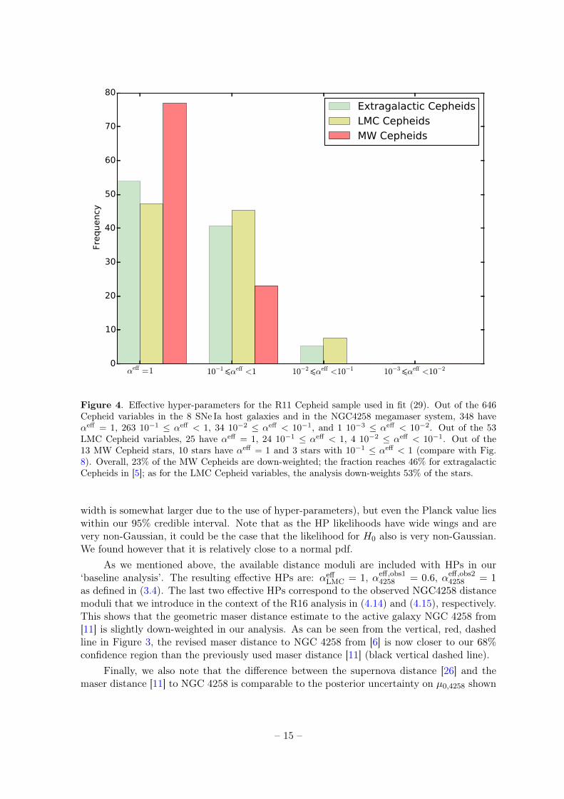
Figure 4. Effective hyper-parameters for the R11 Cepheid sample used in fit (29). Out of the 646Cepheid variables in the 8 SNe Ia host galaxies and in the NGC4258 megamaser system, 348 haveαeff = 1, 263 10−1 ≤ αeff < 1, 34 10−2 ≤ αeff < 10−1, and 1 10−3 ≤ αeff < 10−2. Out of the 53LMC Cepheid variables, 25 have αeff = 1, 24 10−1 ≤ αeff < 1, 4 10−2 ≤ αeff < 10−1. Out of the13 MW Cepheid stars, 10 stars have αeff = 1 and 3 stars with 10−1 ≤ αeff < 1 (compare with Fig.8). Overall, 23% of the MW Cepheids are down-weighted; the fraction reaches 46% for extragalacticCepheids in [5]; as for the LMC Cepheid variables, the analysis down-weights 53% of the stars.
width is somewhat larger due to the use of hyper-parameters), but even the Planck value lieswithin our 95% credible interval. Note that as the HP likelihoods have wide wings and arevery non-Gaussian, it could be the case that the likelihood for H0 also is very non-Gaussian.We found however that it is relatively close to a normal pdf.
As we mentioned above, the available distance moduli are included with HPs in our‘baseline analysis’. The resulting effective HPs are: αeff
LMC = 1, αeff,obs14258 = 0.6, αeff,obs2
4258 = 1as defined in (3.4). The last two effective HPs correspond to the observed NGC4258 distancemoduli that we introduce in the context of the R16 analysis in (4.14) and (4.15), respectively.This shows that the geometric maser distance estimate to the active galaxy NGC 4258 from[11] is slightly down-weighted in our analysis. As can be seen from the vertical, red, dashedline in Figure 3, the revised maser distance to NGC 4258 from [6] is now closer to our 68%confidence region than the previously used maser distance [11] (black vertical dashed line).
Finally, we also note that the difference between the supernova distance [26] and themaser distance [11] to NGC 4258 is comparable to the posterior uncertainty on µ0,4258 shown
– 15 –
13.5 14.0 14.5 15.0 15.5 16.0 16.5 17.0
SN Ia m 0v +5av [mag]
0.0
0.5
1.0
1.5
2.0
2.5
3.0
3.5C
ephei
d(µ
0−µ
0,4
258)
[mag
]Relative distances from Cepheid variables and SNe Ia
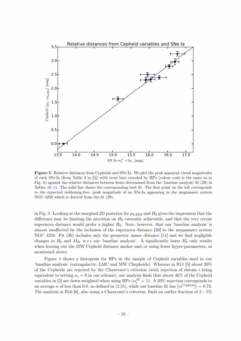
Figure 5. Relative distances from Cepheids and SNe Ia. We plot the peak apparent visual magnitudesof each SNe Ia (from Table 3 in [5]) with error bars rescaled by HPs (colour code is the same as inFig. 6) against the relative distances between hosts determined from the ‘baseline analysis’ fit (29) inTables 10–11. The solid line shows the corresponding best fit. The first point on the left correspondsto the expected reddening-free, peak magnitude of an SNe Ia appearing in the megamaser systemNGC 4258 which is derived from the fit (29).
in Fig. 3. Looking at the marginal 2D posterior for µ0,4258 andH0 gives the impression that thedifference may be limiting the precision on H0 currently achievable, and that the very recentsupernova distance would prefer a higher H0. Note, however, that our ‘baseline analysis’ isalmost unaffected by the inclusion of the supernova distance [26] to the megamaser systemNGC 4258. Fit (30) includes only the geometric maser distance [11] and we find negligiblechanges in H0 and MW w.r.t our ‘baseline analysis’. A significantly lower H0 only resultswhen leaving out the MW Cepheid distance anchor and/or using fewer hyper-parameters, asmentioned above.
Figure 4 shows a histogram for HPs in the sample of Cepheid variables used in our‘baseline analysis’ (extragalactic, LMC and MW Chepheids). Whereas in R11 [5] about 20%of the Cepheids are rejected by the Chauvenet’s criterion (with rejection of datum i beingequivalent to setting αi = 0 in our scheme), our analysis finds that about 46% of the Cepheidvariables in [5] are down-weighted when using HPs (αeff
i < 1). A 20% rejection corresponds toan average α of less than 0.8, as defined in (2.25), while our baseline fit has ||αCepheid|| = 0.72.The analysis in R16 [6], also using a Chauvenet’s criterion, finds an outlier fraction of 2− 5%
– 16 –
in a larger sample of Cepheid variables.Table 1 shows the distance parameters for the SNe Ia hosts of our baseline analysis,
together with the corresponding effective HP and internal scatter for each host. The entrieswith αeff < 1 point to the presence of possible outliers among the sample of SNe Ia hosts,justifying our use of HPs in the apparent visual magnitudes of each SN Ia. This is alsovisible in Figure 5 where the three ‘blue’ supernovae have their error bars enlarged in orderto remain consistent with the global best fit (the diagonal solid line). This could be a hintof unaccounted systematics in the light-curve fits for those SNe Ia. Note that R16 uses adifferent light-curve fitting algorithm (SALT-II) to that utilised in R11 (MLCS2k2) findingno evidence for any of their 19 SNe Ia hosts to be an outlier.
4 Testing assumptions
In this section we look at the choices that we made for the baseline analysis described in theprevious section. Specifically, in Subsection 4.1 we look at the consistency of the Cepheidfits and the distance anchors. In Subsection 4.2 we consider the metallicity dependence ofthe Cepheid fits. In Subsections 4.3 and 4.4 we study to what extent both the period cut-offand inclusion of different kinds of data with HPs make a difference in our analysis. For thissection we use as reference the R11 data. In Section 5 we will then highlight how our ‘baselineanalysis’ changes when analysing the R16 data set with respect to our analysis of R11 dataset.
4.1 Consistency tests for Cepheid distances, using hyper-parameters
In this subsection we take a closer look at the Cepheids in the LMC, the MW, and themegamaser system NGC 4258. This will allow us to show in a simple example how the HPsaffect the analysis, to check whether the Cepheids and anchor distances of these systems arein agreement, and also to compare our outcome with results in [10].
4.1.1 The LMC Cepheid variables
We start out our analysis by applying HPs to the set of 53 Large Magellanic Cloud (LMC)Cepheid variables with H-band magnitudes, mH , listed in Table 3 of [23] and V , I bandmagnitudes, mV , mI , listed in Table 4 of [24]. Following [5, 6, 10], we rely primarily on(near-infrared) NIR ‘Wesenheit reddening-free’ magnitudes, defined as
mW,i = mH,i −R(mV,i −mI,i), (4.1)
where R is a constant defining the reddening law; when analysing the R11 data set, we useR = 0.410 as G. Efstathiou did [10]; when utilising the R16 data set, we study the sensitivityof our results to variations in R. For the purpose of comparing with [10] we neglect for nowmetallicity dependence and fit the data with a period-luminosity relation
mCepheidW (P ) ≡ mP
W = A+ bW (logP − 1) (4.2)
where A = µ0,LMC +MW in notation of Eq. (2.9) and P is the period. In order to apply HPswe use (2.11) as done already in (3.2b) and define
χ2,LMCi =
(mW,i −mPW )2
σ2i + σ2,LMC
int
, (4.3)
– 17 –
LMC Cepheid variablesFit A bW σLMC
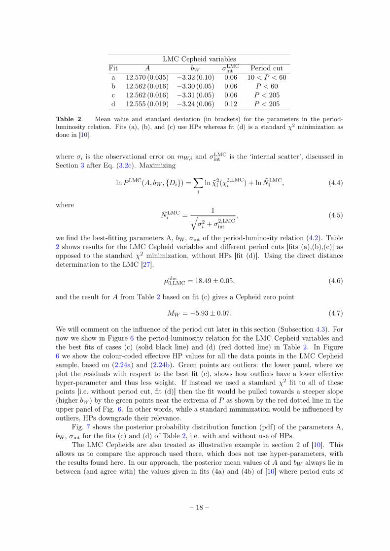
int Period cuta 12.570 (0.035) −3.32 (0.10) 0.06 10 < P < 60b 12.562 (0.016) −3.30 (0.05) 0.06 P < 60c 12.562 (0.016) −3.31 (0.05) 0.06 P < 205d 12.555 (0.019) −3.24 (0.06) 0.12 P < 205
Table 2. Mean value and standard deviation (in brackets) for the parameters in the period-luminosity relation. Fits (a), (b), and (c) use HPs whereas fit (d) is a standard χ2 minimization asdone in [10].
where σi is the observational error on mW,i and σLMCint is the ‘internal scatter’, discussed in
Section 3 after Eq. (3.2c). Maximizing
lnPLMC(A, bW , {Di}) =∑i
ln χ2i (χ
2,LMCi ) + ln NLMC
i , (4.4)
whereNLMCi =
1√σ2i + σ2,LMC
int
, (4.5)
we find the best-fitting parameters A, bW, σint of the period-luminosity relation (4.2). Table2 shows results for the LMC Cepheid variables and different period cuts [fits (a),(b),(c)] asopposed to the standard χ2 minimization, without HPs [fit (d)]. Using the direct distancedetermination to the LMC [27],
µobs0,LMC = 18.49± 0.05, (4.6)
and the result for A from Table 2 based on fit (c) gives a Cepheid zero point
MW = −5.93± 0.07. (4.7)
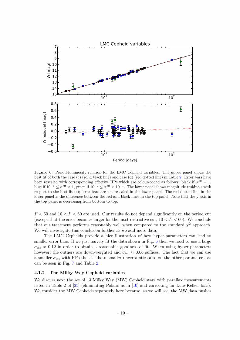
We will comment on the influence of the period cut later in this section (Subsection 4.3). Fornow we show in Figure 6 the period-luminosity relation for the LMC Cepheid variables andthe best fits of cases (c) (solid black line) and (d) (red dotted line) in Table 2. In Figure6 we show the colour-coded effective HP values for all the data points in the LMC Cepheidsample, based on (2.24a) and (2.24b). Green points are outliers: the lower panel, where weplot the residuals with respect to the best fit (c), shows how outliers have a lower effectivehyper-parameter and thus less weight. If instead we used a standard χ2 fit to all of thesepoints [i.e. without period cut, fit (d)] then the fit would be pulled towards a steeper slope(higher bW ) by the green points near the extrema of P as shown by the red dotted line in theupper panel of Fig. 6. In other words, while a standard minimization would be influenced byoutliers, HPs downgrade their relevance.
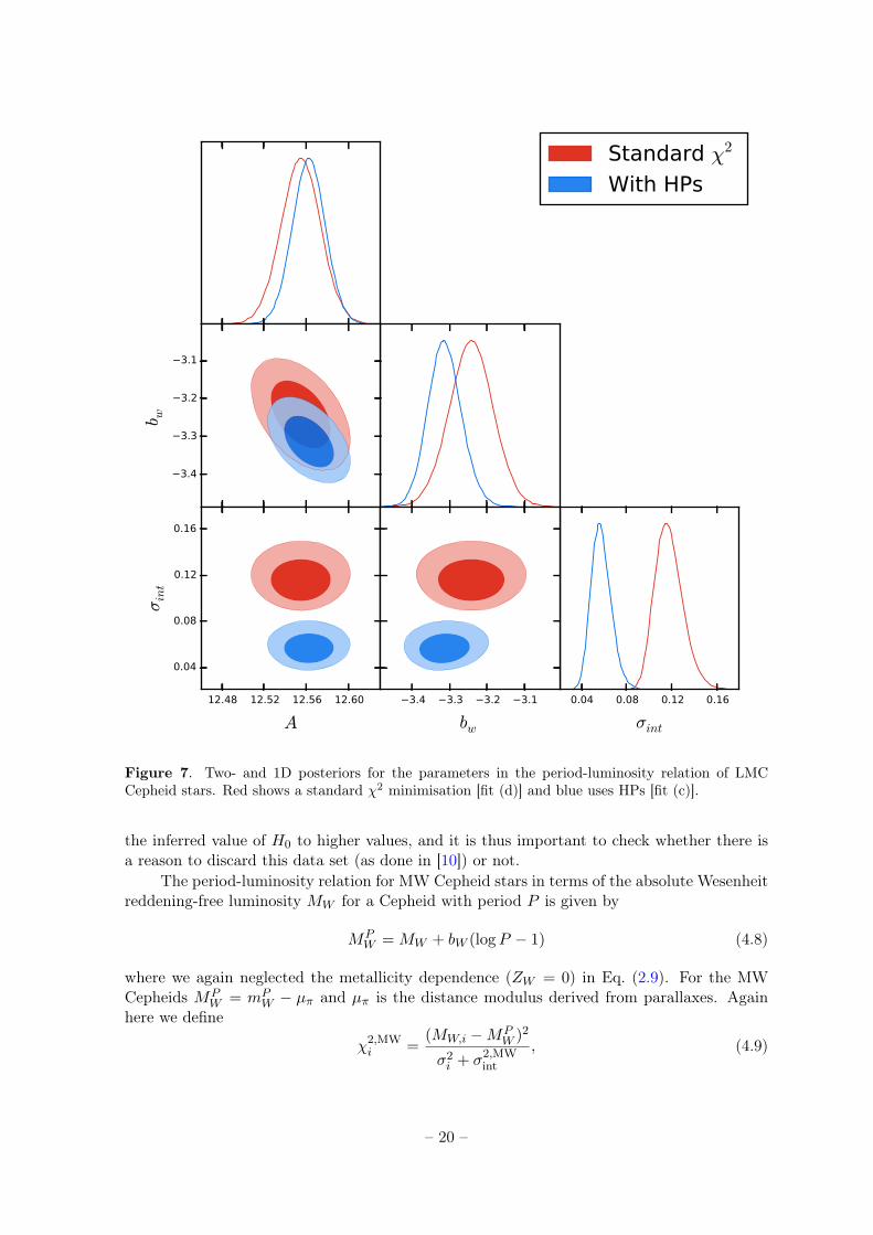
Fig. 7 shows the posterior probability distribution function (pdf) of the parameters A,bW, σint for the fits (c) and (d) of Table 2, i.e. with and without use of HPs.
The LMC Cepheids are also treated as illustrative example in section 2 of [10]. Thisallows us to compare the approach used there, which does not use hyper-parameters, withthe results found here. In our approach, the posterior mean values of A and bW always lie inbetween (and agree with) the values given in fits (4a) and (4b) of [10] where period cuts of
– 18 –
101 102
7
8
9
10
11
12
13
14
15
W [
mag]
LMC Cepheid variables
101 102
Period [days]
0.6
0.4
0.2
0.0
0.2
0.4
0.6
0.8
W r
esi
dual [m
ag]
Figure 6. Period-luminosity relation for the LMC Cepheid variables. The upper panel shows thebest fit of both the case (c) (solid black line) and case (d) (red dotted line) in Table 2. Error bars havebeen rescaled with corresponding effective HPs which are colour-coded as follows: black if αeff = 1,blue if 10−1 ≤ αeff < 1, green if 10−2 ≤ αeff < 10−1. The lower panel shows magnitude residuals withrespect to the best fit (c); error bars are not rescaled in the lower panel. The red dotted line in thelower panel is the difference between the red and black lines in the top panel. Note that the y axis inthe top panel is decreasing from bottom to top.
P < 60 and 10 < P < 60 are used. Our results do not depend significantly on the period cut(except that the error becomes larger for the most restrictive cut, 10 < P < 60). We concludethat our treatment performs reasonably well when compared to the standard χ2 approach.We will investigate this conclusion further as we add more data.
The LMC Cepheids provide a nice illustration of how hyper-parameters can lead tosmaller error bars. If we just naively fit the data shown in Fig. 6 then we need to use a largeσint ≈ 0.12 in order to obtain a reasonable goodness of fit. When using hyper-parametershowever, the outliers are down-weighted and σint ≈ 0.06 suffices. The fact that we can usea smaller σint with HPs then leads to smaller uncertainties also on the other parameters, ascan be seen in Fig. 7 and Table 2.
4.1.2 The Milky Way Cepheid variables
We discuss next the set of 13 Milky Way (MW) Cepheid stars with parallax measurementslisted in Table 2 of [25] (eliminating Polaris as in [10] and correcting for Lutz-Kelker bias).We consider the MW Cepheids separately here because, as we will see, the MW data pushes
– 19 –
0.04 0.08 0.12 0.16
σint
3.4
3.3
3.2
3.1
b w
12.48 12.52 12.56 12.60
A
0.04
0.08
0.12
0.16
σint
3.4 3.3 3.2 3.1
bw
Standard χ2
With HPs
Figure 7. Two- and 1D posteriors for the parameters in the period-luminosity relation of LMCCepheid stars. Red shows a standard χ2 minimisation [fit (d)] and blue uses HPs [fit (c)].
the inferred value of H0 to higher values, and it is thus important to check whether there isa reason to discard this data set (as done in [10]) or not.
The period-luminosity relation for MW Cepheid stars in terms of the absolute Wesenheitreddening-free luminosity MW for a Cepheid with period P is given by
MPW = MW + bW (logP − 1) (4.8)
where we again neglected the metallicity dependence (ZW = 0) in Eq. (2.9). For the MWCepheids MP
W = mPW − µπ and µπ is the distance modulus derived from parallaxes. Again
here we define
χ2,MWi =
(MW,i −MPW )2
σ2i + σ2,MW
int
, (4.9)
– 20 –
101
8.07.57.06.56.05.55.04.54.03.5
MW
[m
ag]
MW Cepheid variables
101
Period [days]
0.6
0.4
0.2
0.0
0.2
0.4
0.6
MW
resi
dual [m
ag]
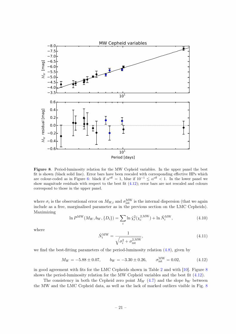
Figure 8. Period-luminosity relation for the MW Cepheid variables. In the upper panel the bestfit is shown (black solid line). Error bars have been rescaled with corresponding effective HPs whichare colour-coded as in Figure 6: black if αeff = 1, blue if 10−1 ≤ αeff < 1. In the lower panel weshow magnitude residuals with respect to the best fit (4.12); error bars are not rescaled and colourscorrespond to those in the upper panel.
where σi is the observational error onMW,i and σMWint is the internal dispersion (that we again
include as a free, marginalised parameter as in the previous section on the LMC Cepheids).Maximizing
lnPMW(MW , bW , {Di}) =∑i
ln χ2i (χ
2,MWi ) + ln NMW
i , (4.10)
whereNMWi =
1√σ2i + σ2,MW
int
, (4.11)
we find the best-fitting parameters of the period-luminosity relation (4.8), given by
MW = −5.88± 0.07, bW = −3.30± 0.26, σMWint = 0.02, (4.12)
in good agreement with fits for the LMC Cepheids shown in Table 2 and with [10]. Figure 8shows the period-luminosity relation for the MW Cepheid variables and the best fit (4.12).
The consistency in both the Cepheid zero point MW (4.7) and the slope bW betweenthe MW and the LMC Cepheid data, as well as the lack of marked outliers visible in Fig. 8
– 21 –
101 102
16
18
20
22
24
26
28
W [
mag]
NGC4258 Cepheid variables
101 102
Period [days]
3
2
1
0
1
2
3
W r
esi
dual [m
ag]
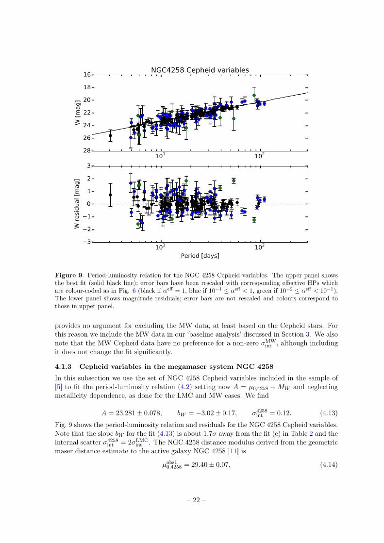
Figure 9. Period-luminosity relation for the NGC 4258 Cepheid variables. The upper panel showsthe best fit (solid black line); error bars have been rescaled with corresponding effective HPs whichare colour-coded as in Fig. 6 (black if αeff = 1, blue if 10−1 ≤ αeff < 1, green if 10−2 ≤ αeff < 10−1).The lower panel shows magnitude residuals; error bars are not rescaled and colours correspond tothose in upper panel.
provides no argument for excluding the MW data, at least based on the Cepheid stars. Forthis reason we include the MW data in our ‘baseline analysis’ discussed in Section 3. We alsonote that the MW Cepheid data have no preference for a non-zero σMW
int , although includingit does not change the fit significantly.
4.1.3 Cepheid variables in the megamaser system NGC 4258
In this subsection we use the set of NGC 4258 Cepheid variables included in the sample of[5] to fit the period-luminosity relation (4.2) setting now A = µ0,4258 + MW and neglectingmetallicity dependence, as done for the LMC and MW cases. We find
A = 23.281± 0.078, bW = −3.02± 0.17, σ4258int = 0.12. (4.13)
Fig. 9 shows the period-luminosity relation and residuals for the NGC 4258 Cepheid variables.Note that the slope bW for the fit (4.13) is about 1.7σ away from the fit (c) in Table 2 and theinternal scatter σ4258
int = 2σLMCint . The NGC 4258 distance modulus derived from the geometric
maser distance estimate to the active galaxy NGC 4258 [11] is
µobs10,4258 = 29.40± 0.07, (4.14)
– 22 –
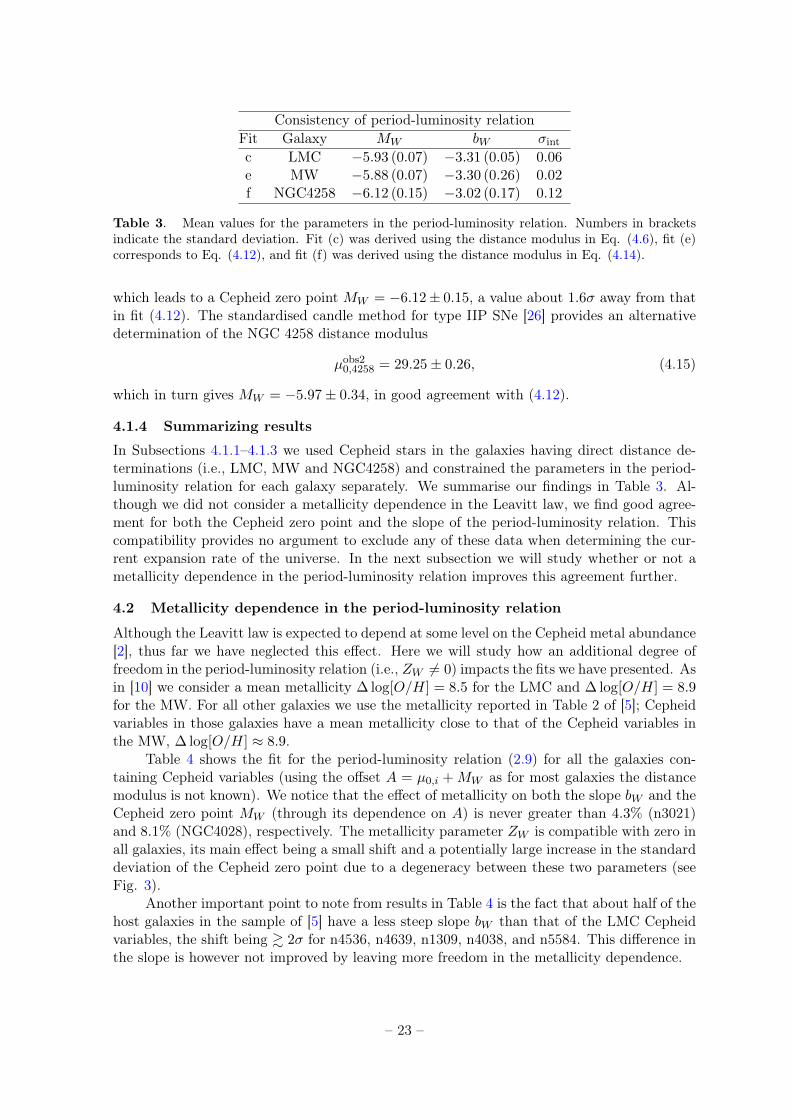
Consistency of period-luminosity relationFit Galaxy MW bW σint
c LMC −5.93 (0.07) −3.31 (0.05) 0.06e MW −5.88 (0.07) −3.30 (0.26) 0.02f NGC4258 −6.12 (0.15) −3.02 (0.17) 0.12
Table 3. Mean values for the parameters in the period-luminosity relation. Numbers in bracketsindicate the standard deviation. Fit (c) was derived using the distance modulus in Eq. (4.6), fit (e)corresponds to Eq. (4.12), and fit (f) was derived using the distance modulus in Eq. (4.14).
which leads to a Cepheid zero point MW = −6.12± 0.15, a value about 1.6σ away from thatin fit (4.12). The standardised candle method for type IIP SNe [26] provides an alternativedetermination of the NGC 4258 distance modulus
µobs20,4258 = 29.25± 0.26, (4.15)
which in turn gives MW = −5.97± 0.34, in good agreement with (4.12).
4.1.4 Summarizing results
In Subsections 4.1.1–4.1.3 we used Cepheid stars in the galaxies having direct distance de-terminations (i.e., LMC, MW and NGC4258) and constrained the parameters in the period-luminosity relation for each galaxy separately. We summarise our findings in Table 3. Al-though we did not consider a metallicity dependence in the Leavitt law, we find good agree-ment for both the Cepheid zero point and the slope of the period-luminosity relation. Thiscompatibility provides no argument to exclude any of these data when determining the cur-rent expansion rate of the universe. In the next subsection we will study whether or not ametallicity dependence in the period-luminosity relation improves this agreement further.
4.2 Metallicity dependence in the period-luminosity relation
Although the Leavitt law is expected to depend at some level on the Cepheid metal abundance[2], thus far we have neglected this effect. Here we will study how an additional degree offreedom in the period-luminosity relation (i.e., ZW 6= 0) impacts the fits we have presented. Asin [10] we consider a mean metallicity ∆ log[O/H] = 8.5 for the LMC and ∆ log[O/H] = 8.9for the MW. For all other galaxies we use the metallicity reported in Table 2 of [5]; Cepheidvariables in those galaxies have a mean metallicity close to that of the Cepheid variables inthe MW, ∆ log[O/H] ≈ 8.9.
Table 4 shows the fit for the period-luminosity relation (2.9) for all the galaxies con-taining Cepheid variables (using the offset A = µ0,i + MW as for most galaxies the distancemodulus is not known). We notice that the effect of metallicity on both the slope bW and theCepheid zero point MW (through its dependence on A) is never greater than 4.3% (n3021)and 8.1% (NGC4028), respectively. The metallicity parameter ZW is compatible with zero inall galaxies, its main effect being a small shift and a potentially large increase in the standarddeviation of the Cepheid zero point due to a degeneracy between these two parameters (seeFig. 3).
Another important point to note from results in Table 4 is the fact that about half of thehost galaxies in the sample of [5] have a less steep slope bW than that of the LMC Cepheidvariables, the shift being & 2σ for n4536, n4639, n1309, n4038, and n5584. This difference inthe slope is however not improved by leaving more freedom in the metallicity dependence.
– 23 –
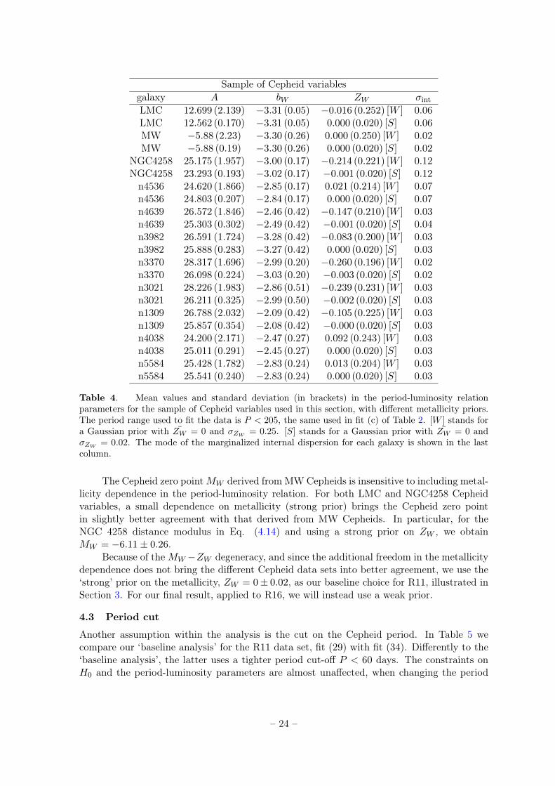
Sample of Cepheid variablesgalaxy A bW ZW σint
LMC 12.699 (2.139) −3.31 (0.05) −0.016 (0.252) [W ] 0.06LMC 12.562 (0.170) −3.31 (0.05) 0.000 (0.020) [S] 0.06MW −5.88 (2.23) −3.30 (0.26) 0.000 (0.250) [W ] 0.02MW −5.88 (0.19) −3.30 (0.26) 0.000 (0.020) [S] 0.02
NGC4258 25.175 (1.957) −3.00 (0.17) −0.214 (0.221) [W ] 0.12NGC4258 23.293 (0.193) −3.02 (0.17) −0.001 (0.020) [S] 0.12n4536 24.620 (1.866) −2.85 (0.17) 0.021 (0.214) [W ] 0.07n4536 24.803 (0.207) −2.84 (0.17) 0.000 (0.020) [S] 0.07n4639 26.572 (1.846) −2.46 (0.42) −0.147 (0.210) [W ] 0.03n4639 25.303 (0.302) −2.49 (0.42) −0.001 (0.020) [S] 0.04n3982 26.591 (1.724) −3.28 (0.42) −0.083 (0.200) [W ] 0.03n3982 25.888 (0.283) −3.27 (0.42) 0.000 (0.020) [S] 0.03n3370 28.317 (1.696) −2.99 (0.20) −0.260 (0.196) [W ] 0.02n3370 26.098 (0.224) −3.03 (0.20) −0.003 (0.020) [S] 0.02n3021 28.226 (1.983) −2.86 (0.51) −0.239 (0.231) [W ] 0.03n3021 26.211 (0.325) −2.99 (0.50) −0.002 (0.020) [S] 0.03n1309 26.788 (2.032) −2.09 (0.42) −0.105 (0.225) [W ] 0.03n1309 25.857 (0.354) −2.08 (0.42) −0.000 (0.020) [S] 0.03n4038 24.200 (2.171) −2.47 (0.27) 0.092 (0.243) [W ] 0.03n4038 25.011 (0.291) −2.45 (0.27) 0.000 (0.020) [S] 0.03n5584 25.428 (1.782) −2.83 (0.24) 0.013 (0.204) [W ] 0.03n5584 25.541 (0.240) −2.83 (0.24) 0.000 (0.020) [S] 0.03
Table 4. Mean values and standard deviation (in brackets) in the period-luminosity relationparameters for the sample of Cepheid variables used in this section, with different metallicity priors.The period range used to fit the data is P < 205, the same used in fit (c) of Table 2. [W ] stands fora Gaussian prior with ZW = 0 and σZW
= 0.25. [S] stands for a Gaussian prior with ZW = 0 andσZW
= 0.02. The mode of the marginalized internal dispersion for each galaxy is shown in the lastcolumn.
The Cepheid zero pointMW derived fromMWCepheids is insensitive to including metal-licity dependence in the period-luminosity relation. For both LMC and NGC4258 Cepheidvariables, a small dependence on metallicity (strong prior) brings the Cepheid zero pointin slightly better agreement with that derived from MW Cepheids. In particular, for theNGC 4258 distance modulus in Eq. (4.14) and using a strong prior on ZW , we obtainMW = −6.11± 0.26.
Because of theMW −ZW degeneracy, and since the additional freedom in the metallicitydependence does not bring the different Cepheid data sets into better agreement, we use the‘strong’ prior on the metallicity, ZW = 0± 0.02, as our baseline choice for R11, illustrated inSection 3. For our final result, applied to R16, we will instead use a weak prior.
4.3 Period cut
Another assumption within the analysis is the cut on the Cepheid period. In Table 5 wecompare our ‘baseline analysis’ for the R11 data set, fit (29) with fit (34). Differently to the‘baseline analysis’, the latter uses a tighter period cut-off P < 60 days. The constraints onH0 and the period-luminosity parameters are almost unaffected, when changing the period
– 24 –
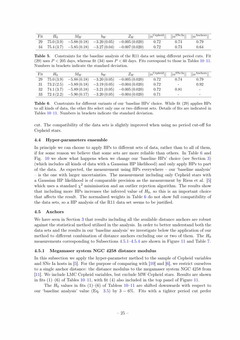
Fit H0 MW bW ZW ||αCepheid|| ||αSNe Ia|| ||αAnchors||29 75.0 (3.9) −5.88 (0.18) −3.20 (0.05) −0.005 (0.020) 0.72 0.74 0.7934 75.4 (3.7) −5.85 (0.18) −3.27 (0.04) −0.007 (0.020) 0.72 0.73 0.64
Table 5. Constraints for the baseline analysis of the R11 data set using different period cuts. Fit(29) uses P < 205 days, whereas fit (34) uses P < 60 days. Fits correspond to those in Tables 10–11.Numbers in brackets indicate the standard deviation.
Fit H0 MW bW ZW ||αCepheid|| ||αSNe Ia|| ||αAnchors||29 75.0 (3.9) −5.88 (0.18) −3.20 (0.05) −0.005 (0.020) 0.72 0.74 0.7931 73.2 (2.5) −5.89 (0.18) −3.19 (0.05) −0.004 (0.020) 0.72 - 0.9232 74.1 (3.7) −5.89 (0.18) −3.21 (0.05) −0.005 (0.020) 0.72 0.81 -33 72.4 (2.2) −5.90 (0.17) −3.20 (0.05) −0.004 (0.020) 0.71 - -
Table 6. Constraints for different variants of our ‘baseline HPs’ choice. While fit (29) applies HPsto all kinds of data, the other fits select only one or two different sets. Details of fits are indicated inTables 10–11. Numbers in brackets indicate the standard deviation.
cut. The compatibility of the data sets is slightly improved when using no period cut-off forCepheid stars.
4.4 Hyper-parameters ensemble
In principle we can choose to apply HPs to different sets of data, rather than to all of them,if for some reason we believe that some sets are more reliable than others. In Table 6 andFig. 10 we show what happens when we change our ‘baseline HPs’ choice (see Section 3)(which includes all kinds of data with a Gaussian HP likelihood) and only apply HPs to partof the data. As expected, the measurement using HPs everywhere – our ‘baseline analysis’– is the one with larger uncertainties. The measurement including only Cepheid stars witha Gaussian HP likelihood is of comparable precision as the measurement by Riess et al. [5]which uses a standard χ2 minimisation and an outlier rejection algorithm. The results showthat including more HPs increases the inferred value of H0, so this is an important choicethat affects the result. The normalised weights in Table 6 do not show full compatibility ofthe data sets, so a HP analysis of the R11 data set seems to be justified.
4.5 Anchors
We have seen in Section 3 that results including all the available distance anchors are robustagainst the statistical method utilised in the analysis. In order to better understand both thedata sets and the results in our ‘baseline analysis’ we investigate below the application of ourmethod to different combination of distance anchors excluding one or two of them. The H0
measurements corresponding to Subsections 4.5.1–4.5.4 are shown in Figure 11 and Table 7.
4.5.1 Megamaser system NGC 4258 distance modulus
In this subsection we apply the hyper-parameter method to the sample of Cepheid variablesand SNe Ia hosts in [5]. For the purpose of comparing with [10] and [6], we restrict ourselvesto a single anchor distance: the distance modulus to the megamaser system NGC 4258 from[11]. We include LMC Cepheid variables, but exclude MW Cepheid stars. Results are shownin fits (1)–(6) of Tables 10–11, with fit (4) also included in the top panel of Figure 11.
The H0 values in fits (1)–(6) of Tabless 10–11 are shifted downwards with respect toour ‘baseline analysis’ value (Eq. 3.5) by 3 − 6%. Fits with a tighter period cut prefer
– 25 –
66 68 70 72 74 76 78 80H0 [km/s/Mpc]
Planck 2015 (1.4%)
Riess et al. 2011 (3.3%)
Efstathiou 2014 (3 anchors) (3.4%)
Cardona et al. 2016 (5.2%) [R11 data with 722 HP]
Cardona et al. 2016 (3.4%) [R11 data with 714 HP]
Cardona et al. 2016 (5.0%) [R11 data with 720 HP]
Cardona et al. 2016 (3.0%) [R11 data with 712 HP]
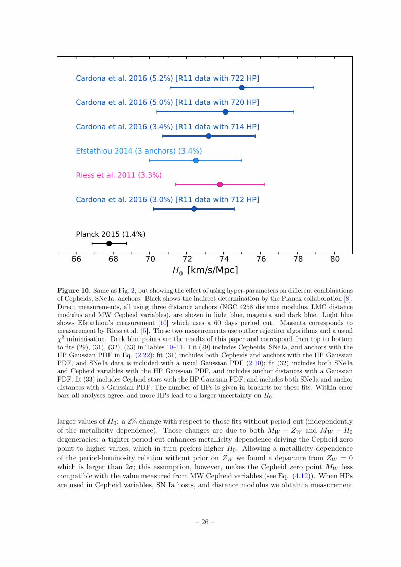
Figure 10. Same as Fig. 2, but showing the effect of using hyper-parameters on different combinationsof Cepheids, SNe Ia, anchors. Black shows the indirect determination by the Planck collaboration [8].Direct measurements, all using three distance anchors (NGC 4258 distance modulus, LMC distancemodulus and MW Cepheid variables), are shown in light blue, magenta and dark blue. Light blueshows Efstathiou’s measurement [10] which uses a 60 days period cut. Magenta corresponds tomeasurement by Riess et al. [5]. These two measurements use outlier rejection algorithms and a usualχ2 minimisation. Dark blue points are the results of this paper and correspond from top to bottomto fits (29), (31), (32), (33) in Tables 10–11. Fit (29) includes Cepheids, SNe Ia, and anchors with theHP Gaussian PDF in Eq. (2.22); fit (31) includes both Cepheids and anchors with the HP GaussianPDF, and SNe Ia data is included with a usual Gaussian PDF (2.10); fit (32) includes both SNe Iaand Cepheid variables with the HP Gaussian PDF, and includes anchor distances with a GaussianPDF; fit (33) includes Cepheid stars with the HP Gaussian PDF, and includes both SNe Ia and anchordistances with a Gaussian PDF. The number of HPs is given in brackets for these fits. Within errorbars all analyses agree, and more HPs lead to a larger uncertainty on H0.
larger values of H0: a 2% change with respect to those fits without period cut (independentlyof the metallicity dependence). Those changes are due to both MW − ZW and MW − H0
degeneracies: a tighter period cut enhances metallicity dependence driving the Cepheid zeropoint to higher values, which in turn prefers higher H0. Allowing a metallicity dependenceof the period-luminosity relation without prior on ZW we found a departure from ZW = 0which is larger than 2σ; this assumption, however, makes the Cepheid zero point MW lesscompatible with the value measured from MW Cepheid variables (see Eq. (4.12)). When HPsare used in Cepheid variables, SN Ia hosts, and distance modulus we obtain a measurement
– 26 –
66 68 70 72 74 76 78 80 82
4.0%4.7%
3.5%
5.8%
NGC 4258WMAP 2009 (3.1%) HPs in Cepheids and SN Ia
66 68 70 72 74 76 78 80 82
5.3%4.2%
3.7%
5.4%
LMCPLANCK 2015 (1.4%)
66 68 70 72 74 76 78 80 82
3.4%4.6%
3.1%
5.6%
MWRiess et al. 2011
66 68 70 72 74 76 78 80 82
3.2%3.6%
5.6%
NGC 4258 + LMCEfstathiou 2015
66 68 70 72 74 76 78 80 82H0 [km/s/Mpc]
3.1%3.9%
2.6%
5.2%
NGC 4258 + MWRiess et al. 2016
66 68 70 72 74 76 78 80 82H0 [km/s/Mpc]
3.2%3.7%
5.0%
LMC + MWHPs in Cepheids, SN Ia, and distance modulus
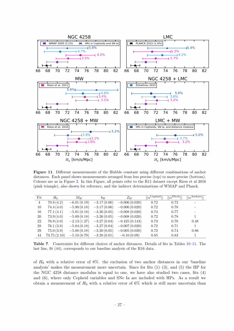
Figure 11. Different measurements of the Hubble constant using different combinations of anchordistances. Each panel shows measurements arranged from less precise (top) to more precise (bottom).Colours are as in Figure 2. In this Figure, all points refer to the R11 dataset except Riess et al 2016(pink triangle), also shown for reference, and the indirect determinations of WMAP and Planck.
Fit H0 MW bW ZW ||αCepheid|| ||αSNe Ia|| ||αAnchors||4 70.8 (4.2) −6.01 (0.19) −3.17 (0.06) −0.006 (0.020) 0.72 0.72 -10 74.4 (4.0) −5.90 (0.18) −3.17 (0.06) −0.006 (0.020) 0.72 0.78 -16 77.1 (4.1) −5.81 (0.18) −3.26 (0.05) −0.008 (0.020) 0.74 0.77 -20 73.9 (4.0) −5.89 (0.18) −3.26 (0.05) −0.008 (0.020) 0.72 0.78 122 76.9 (4.0) −2.13 (1.27) −3.27 (0.04) −0.425 (0.143) 0.73 0.70 0.4828 76.1 (3.8) −5.84 (0.18) −3.27 (0.04) −0.007 (0.020) 0.72 0.71 129 75.0 (3.9) −5.88 (0.18) −3.20 (0.05) −0.005 (0.020) 0.72 0.74 0.8644 73.75 (2.10) −5.10 (0.79) −3.28 (0.01) −0.10 (0.09) 0.85 0.83 1
Table 7. Constraints for different choices of anchor distances. Details of fits in Tables 10–11. Thelast line, fit (44), corresponds to our baseline analysis of the R16 data.
of H0 with a relative error of 8%: the exclusion of two anchor distances in our ‘baselineanalysis’ makes the measurement more uncertain. Since for fits (1)–(3), and (5) the HP forthe NGC 4258 distance modulus is equal to one, we have also studied two cases, fits (4)and (6), where only Cepheid variables and SNe Ia are included with HPs. As a result weobtain a measurement of H0 with a relative error of 6% which is still more uncertain than
– 27 –
the corresponding case using the three anchor distances.In the upper left panel of Figure 11 we show H0 value from fit (4) in Tables 10–11,
together with the values found by Riess et al. [5] (H0 = 74.8±3.0 km s−1 Mpc−1) which did notuse the revised distance modulus from [11], Efstathiou [10] (H0 = 70.6± 3.3 km s−1 Mpc−1),Riess et al. [6] (H0 = 72.25±2.51 km s−1 Mpc−1) which used a redetermination of the distancemodulus to NGC 4258. Our value is compatible with all previous direct determinations of H0
and also with the indirect determinations from Planck and WMAP. The measurement usingHPs is the most uncertain among the direct measurements due to inclusion of SNe Ia withHPs. The Planck collaboration used Efstathiou’s value as a prior for H0 when combiningCMB measurements and local measurements of the Hubble constant. The choice of H0 prioris important as a discrepancy between high and low redshifts in the ΛCDM model could pointto new physics and change conclusions for the extended models discussed e.g. in the Planckpublications [8, 29].
4.5.2 LMC distance modulus
In this subsection we apply our method to the sample of Cepheid variables and SNe Ia hosts in[5], but restrict ourselves to a single anchor distance: the distance modulus to the LMC from[27]. We also include NGC4258 Cepheid variables, but omit MW Cepheid variables. Resultsare shown in fits (7)–(12) of Tables 10–11 and fit (10) is shown in the top-right panel of Fig.11. We have examined different period cuts and different assumptions for the metallicitydependence in the Leavitt Law.
The fits (7)–(12) in Tables 10–11 show a 0 − 7% shift in H0 w.r.t the value in Eq.(3.5). A period cut shifts H0 values by 0.7 − 2% (w.r.t. fits without period cut), whereasthe use of HPs in LMC distance modulus changes H0 values by . 0.4%. Fits (7)–(12) inTables 10–11 represent 5 − 7% measurements of the Hubble constant. In upper right panelof Figure 11 we show H0 value of fit (10) along with measurements by Riess et al. [5](H0 = 71.3 ± 3.8 km s−1 Mpc−1), Efstathiou [10] (H0 = 73.4 ± 3.1 km s−1 Mpc−1), Riess etal. [6] (H0 = 72.04 ± 2.67 km s−1 Mpc−1). Our measurement is almost as precise as that of[5] and is in good agreement with all the other direct determinations of the Hubble constant.While the WMAP value agrees at 1σ level with ours, the Planck value agrees at 2σ level.
4.5.3 Parallax measurements of Cepheid variables in the Milky Way
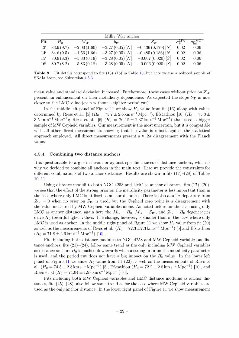
Parallax measurements of Cepheid variables (see Subsection 4.1.2) in our galaxy are usedin this section as the sole anchor distance scale. We include Cepheid variables in both themegamaser system NGC 4258 and those in the LMC. We show the resulting constraints infits (13)–(16) of Tables 10–11. In addition to different period cuts and different assumptionsfor the metallicity dependence in the Leavitt Law, we have included some cases (see Table 8)where those hosts galaxies whose slope bW departs from the LMC value (fit (c) in Table 2)by & 2σ are excluded from the fit.
Fits (13)–(16) in Tables 10–11 are shifted upwards w.r.t our ’baseline analysis’ by 3−4%.In this case we obtain a 5 − 6% measurement of the Hubble constant. A tighter period cutin the Leavitt Law shifts H0 values by 0.3− 0.4% (w.r.t. fits without period cut). A strongprior on the metallicity parameter ZW drives downwards H0 by 1 − 2% (w.r.t. fits withno prior). When including the metallicity dependence without a prior we observe a slightbW −H0 degeneracy: less negative bW prefers higher H0 values. Fits (13l)–(16l) in Table 8do not include Cepheid variables in galaxy hosts with a slope bW differing & 2σ from theLMC value (see Subsection 4.2). The main impact of this change is seen in H0 having both
– 28 –
Milky Way anchorFit H0 MW bW ZW σMW
int σLMCint
13l 83.9 (9.7) −2.00 (1.60) −3.27 (0.05) [N ] −0.436 (0.179) [N ] 0.02 0.0614l 84.6 (9.5) −1.56 (1.66) −3.27 (0.05) [N ] −0.485 (0.186) [N ] 0.02 0.0615l 80.9 (8.3) −5.83 (0.19) −3.28 (0.05) [N ] −0.007 (0.020) [S] 0.02 0.0616l 80.7 (8.2) −5.83 (0.18) −3.28 (0.05) [N ] −0.006 (0.020) [S] 0.02 0.06
Table 8. Fit details correspond to fits (13)–(16) in Table 10, but here we use a reduced sample ofSNe Ia hosts, see Subsection 4.5.3.
mean value and standard deviation increased. Furthermore, those cases without prior on ZWpresent an enhancement on their metallicity dependence. As expected the slope bW is nowcloser to the LMC value (even without a tighter period cut).
In the middle left panel of Figure 11 we show H0 value from fit (16) along with valuesdetermined by Riess et al. [5] (H0 = 75.7± 2.6 km s−1 Mpc−1); Efstathiou [10] (H0 = 75.3±3.5 km s−1 Mpc−1); Riess et al. [6] (H0 = 76.18 ± 2.37 km s−1 Mpc−1) that used a biggersample of MWCepheid variables. Our measurement is the most uncertain, but it is compatiblewith all other direct measurements showing that the value is robust against the statisticalapproach employed. All direct measurements present a ≈ 2σ disagreement with the Planckvalue.
4.5.4 Combining two distance anchors
It is questionable to argue in favour or against specific choices of distance anchors, which iswhy we decided to combine all anchors in the main text. Here we provide the constraints fordifferent combinations of two anchor distances. Results are shown in fits (17)–(28) of Tables10–11.
Using distance moduli to both NGC 4258 and LMC as anchor distances, fits (17)–(20),we see that the effect of the strong prior on the metallicity parameter is less important than inthe case where only LMC is utilised as anchor distance. There is also a ≈ 2σ departure fromZW = 0 when no prior on ZW is used, but the Cepheid zero point is is disagreement withthe value measured by MW Cepheid variables alone. As noted before for the case using onlyLMC as anchor distance, again here the MW −H0, MW − ZW , and ZW −H0 degeneraciesdrive H0 towards higher values. The change, however, is smaller than in the case where onlyLMC is used as anchor. In the middle right panel of Figure 11 we show H0 value from fit (20)as well as the measurements of Riess et al. (H0 = 72.3±2.3 km s−1 Mpc−1) [5] and Efstathiou(H0 = 71.8± 2.6 km s−1 Mpc−1) [10].
Fits including both distance modulus to NGC 4258 and MW Cepheid variables as dis-tance anchors, fits (21)–(24), follow same trend as fits only including MW Cepheid variablesas distance anchor: H0 is pushed downwards when a strong prior on the metallicity parameteris used, and the period cut does not have a big impact on the H0 value. In the lower leftpanel of Figure 11 we show H0 value from fit (22) as well as the measurements of Riess etal. (H0 = 74.5± 2.3 km s−1 Mpc−1) [5], Efstathiou (H0 = 72.2± 2.8 km s−1 Mpc−1) [10], andRiess et al (H0 = 74.04± 1.93 km s−1 Mpc−1) [6].
Fits including both MW Cepheid variables and LMC distance modulus as anchor dis-tances, fits (25)–(28), also follow same trend as for the case where MW Cepheid variables areused as the only anchor distance. In the lower right panel of Figure 11 we show measurement
– 29 –
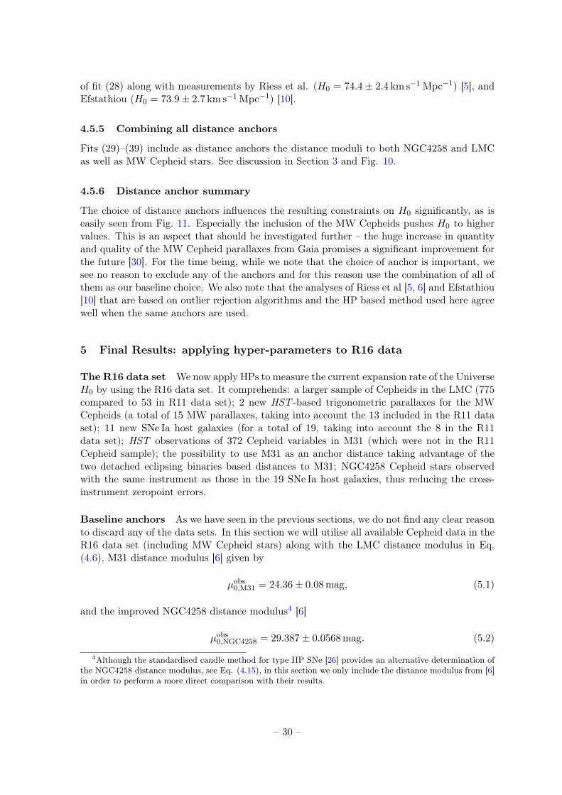
of fit (28) along with measurements by Riess et al. (H0 = 74.4± 2.4 km s−1 Mpc−1) [5], andEfstathiou (H0 = 73.9± 2.7 km s−1 Mpc−1) [10].
4.5.5 Combining all distance anchors
Fits (29)–(39) include as distance anchors the distance moduli to both NGC4258 and LMCas well as MW Cepheid stars. See discussion in Section 3 and Fig. 10.
4.5.6 Distance anchor summary
The choice of distance anchors influences the resulting constraints on H0 significantly, as iseasily seen from Fig. 11. Especially the inclusion of the MW Cepheids pushes H0 to highervalues. This is an aspect that should be investigated further – the huge increase in quantityand quality of the MW Cepheid parallaxes from Gaia promises a significant improvement forthe future [30]. For the time being, while we note that the choice of anchor is important, wesee no reason to exclude any of the anchors and for this reason use the combination of all ofthem as our baseline choice. We also note that the analyses of Riess et al [5, 6] and Efstathiou[10] that are based on outlier rejection algorithms and the HP based method used here agreewell when the same anchors are used.
5 Final Results: applying hyper-parameters to R16 data
The R16 data set We now apply HPs to measure the current expansion rate of the UniverseH0 by using the R16 data set. It comprehends: a larger sample of Cepheids in the LMC (775compared to 53 in R11 data set); 2 new HST -based trigonometric parallaxes for the MWCepheids (a total of 15 MW parallaxes, taking into account the 13 included in the R11 dataset); 11 new SNe Ia host galaxies (for a total of 19, taking into account the 8 in the R11data set); HST observations of 372 Cepheid variables in M31 (which were not in the R11Cepheid sample); the possibility to use M31 as an anchor distance taking advantage of thetwo detached eclipsing binaries based distances to M31; NGC4258 Cepheid stars observedwith the same instrument as those in the 19 SNe Ia host galaxies, thus reducing the cross-instrument zeropoint errors.
Baseline anchors As we have seen in the previous sections, we do not find any clear reasonto discard any of the data sets. In this section we will utilise all available Cepheid data in theR16 data set (including MW Cepheid stars) along with the LMC distance modulus in Eq.(4.6), M31 distance modulus [6] given by
µobs0,M31 = 24.36± 0.08 mag, (5.1)
and the improved NGC4258 distance modulus4 [6]
µobs0,NGC4258 = 29.387± 0.0568 mag. (5.2)
4Although the standardised candle method for type IIP SNe [26] provides an alternative determination ofthe NGC4258 distance modulus, see Eq. (4.15), in this section we only include the distance modulus from [6]in order to perform a more direct comparison with their results.
– 30 –
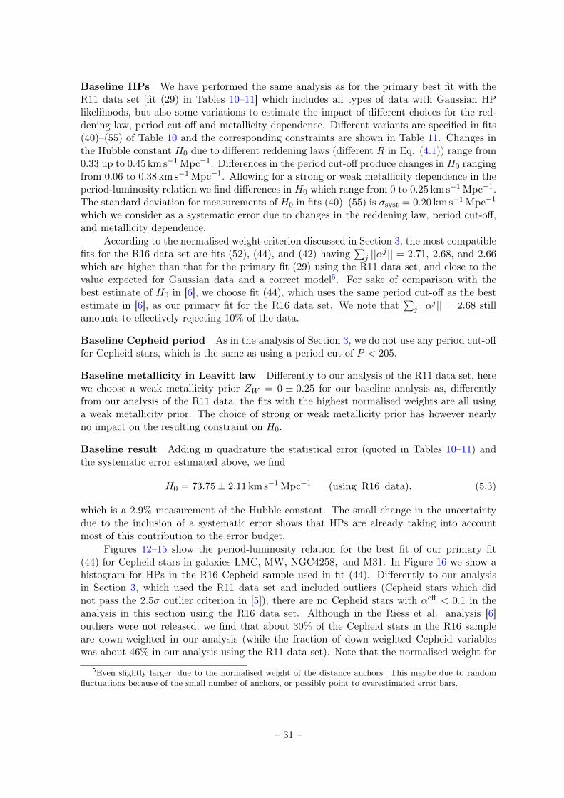
Baseline HPs We have performed the same analysis as for the primary best fit with theR11 data set [fit (29) in Tables 10–11] which includes all types of data with Gaussian HPlikelihoods, but also some variations to estimate the impact of different choices for the red-dening law, period cut-off and metallicity dependence. Different variants are specified in fits(40)–(55) of Table 10 and the corresponding constraints are shown in Table 11. Changes inthe Hubble constant H0 due to different reddening laws (different R in Eq. (4.1)) range from0.33 up to 0.45 km s−1 Mpc−1. Differences in the period cut-off produce changes in H0 rangingfrom 0.06 to 0.38 km s−1 Mpc−1. Allowing for a strong or weak metallicity dependence in theperiod-luminosity relation we find differences in H0 which range from 0 to 0.25 km s−1 Mpc−1.The standard deviation for measurements of H0 in fits (40)–(55) is σsyst = 0.20 km s−1 Mpc−1
which we consider as a systematic error due to changes in the reddening law, period cut-off,and metallicity dependence.
According to the normalised weight criterion discussed in Section 3, the most compatiblefits for the R16 data set are fits (52), (44), and (42) having
∑j ||αj || = 2.71, 2.68, and 2.66
which are higher than that for the primary fit (29) using the R11 data set, and close to thevalue expected for Gaussian data and a correct model5. For sake of comparison with thebest estimate of H0 in [6], we choose fit (44), which uses the same period cut-off as the bestestimate in [6], as our primary fit for the R16 data set. We note that
∑j ||αj || = 2.68 still
amounts to effectively rejecting 10% of the data.
Baseline Cepheid period As in the analysis of Section 3, we do not use any period cut-offfor Cepheid stars, which is the same as using a period cut of P < 205.
Baseline metallicity in Leavitt law Differently to our analysis of the R11 data set, herewe choose a weak metallicity prior ZW = 0 ± 0.25 for our baseline analysis as, differentlyfrom our analysis of the R11 data, the fits with the highest normalised weights are all usinga weak metallicity prior. The choice of strong or weak metallicity prior has however nearlyno impact on the resulting constraint on H0.
Baseline result Adding in quadrature the statistical error (quoted in Tables 10–11) andthe systematic error estimated above, we find
H0 = 73.75± 2.11 km s−1 Mpc−1 (using R16 data), (5.3)
which is a 2.9% measurement of the Hubble constant. The small change in the uncertaintydue to the inclusion of a systematic error shows that HPs are already taking into accountmost of this contribution to the error budget.
Figures 12–15 show the period-luminosity relation for the best fit of our primary fit(44) for Cepheid stars in galaxies LMC, MW, NGC4258, and M31. In Figure 16 we show ahistogram for HPs in the R16 Cepheid sample used in fit (44). Differently to our analysisin Section 3, which used the R11 data set and included outliers (Cepheid stars which didnot pass the 2.5σ outlier criterion in [5]), there are no Cepheid stars with αeff < 0.1 in theanalysis in this section using the R16 data set. Although in the Riess et al. analysis [6]outliers were not released, we find that about 30% of the Cepheid stars in the R16 sampleare down-weighted in our analysis (while the fraction of down-weighted Cepheid variableswas about 46% in our analysis using the R11 data set). Note that the normalised weight for
5Even slightly larger, due to the normalised weight of the distance anchors. This maybe due to randomfluctuations because of the small number of anchors, or possibly point to overestimated error bars.
– 31 –
101 102
7
8
9
10
11
12
13
14
15
W [
mag]
LMC Cepheid variables
101 102
Period [days]
0.4
0.3
0.2
0.1
0.0
0.1
0.2
0.3
0.4
W r
esi
dual [m
ag]
Figure 12. Period-luminosity relation (upper panel) and magnitude residuals for the LMC Cepheidvariables in the R16 data set. The solid line shows the best fit of fit (44). In the upper panel werescale error bars with HPs, in the lower panel we do not. Data are colour-coded as explained inFigure 6.
Cepheids increases from 0.72 for the primary best fit (29) (with the R11 data set) to 0.85for the primary best fit (44) (with the R16 data set), which agrees with the expectations forGaussian data without outliers.
Riess et al. [6] used the SALT-II light curve fitter and found no outliers among the SNe Iahosts. Although we cannot claim the opposite, we do find that some of the SNe Ia are down-weighted in our analysis. In Figure 17 we compare the SNe Ia distances to the approximate,independent Cepheid distances from our primary fit (44). In Table 9 we show the distanceparameters and the HPs for the SNe Ia hosts in the R16 data set. The down-weighted SNe Iahosts might indicate the presence of unaccounted (or underestimated) systematics in the R16data set. Whereas our analysis in Section 3 using the R11 data set showed that three outof the eight host galaxies are down-weighted in the fit, the primary fit (44) using the R16data set down-weights eight SNe Ia host galaxies. The two host galaxies n3982 and n5584 aredown-weighted in both fit (29) and fit (43). From Tables 10–11 we see that the normalisedweight for SNe Ia data is higher for the R16 data set (0.83) in comparison to the R11 dataset (0.74). This indicates an improvement in the compatibility of this kind of data in the R16sample.
If we compare the normalised weight of anchors in Tables 10–11 for fits (29) and (44)
– 32 –
101
9
8
7
6
5
4
3
MW
[m
ag]
MW Cepheid variables
101
Period [days]
0.4
0.2
0.0
0.2
0.4
0.6
MW
resi
dual [m
ag]
Figure 13. Period-luminosity relation (upper panel) and magnitude residuals for the MW Cepheidvariables in the R16 data set. The solid line shows the best fit of fit (44). In the upper panel werescale error bars with HPs, in the lower panel we do not. Data are colour-coded as explained inFigure 6.
(0.86 and 1, respectively), we can also see an improvement in the compatibility of this kindof data in the R16 data set. Although this would suggest not to include distance moduli withHPs in the fit (since the HP Gaussian likelihood would add uncertainty because of its slightlywider wings), the normalised weight of anchors depends on the variants of the analysis (R,period cut-off, metallicity prior) ranging from 0.62 to 1. Hence, there is no strong reason toexclude the use of HPs in this kind of data.
Figure 2 shows the best estimates of H0 by G. Efstathiou [10], Riess et al. [5], Riess etal. [6], and those in this work, fits (29) and (44), along with the indirect determinations of H0
by the WMAP team [7] and by the Planck collaboration [8]. Our best estimate using the R11data set, fit (29), is 75± 3.9km s−1 Mpc−1 and is the most uncertain (a 5.2% measurement)of all presented measurements, but it agrees with all previous direct determinations of H0
and differs by 1.8σ from the Planck value 2015 and 2σ from the updated Planck 2016 value66.93± 0.62 km s−1 Mpc−1 [9]. Note that because G. Efstathiou considered only NGC4258 asan anchor and set a period cut-off of 60 days, his determination is more uncertain than thatof Riess et al. [5] which used three anchors and no period cut-off. As illustrated in the figure(top panel), our best estimate using the R16 data set, fit (44), also agrees with the previousdeterminations of H0, while its uncertainty is smaller (a 2.9% measurement) than the one
– 33 –
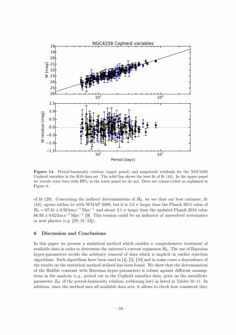
101 102
18
19
20
21
22
23
24
25
26
W [
mag]
NGC4258 Cepheid variables
101 102
Period [days]
1.5
1.0
0.5
0.0
0.5
1.0
1.5
W r
esi
dual [m
ag]
Figure 14. Period-luminosity relation (upper panel) and magnitude residuals for the NGC4258Cepheid variables in the R16 data set. The solid line shows the best fit of fit (44). In the upper panelwe rescale error bars with HPs, in the lower panel we do not. Data are colour-coded as explained inFigure 6.
of fit (29). Concerning the indirect determinations of H0, we see that our best estimate, fit(44), agrees within 1σ with WMAP 2009, but it is 2.6 σ larger than the Planck 2015 value ofH0 = 67.81± 0.92 km s−1 Mpc−1 and about 3.1 σ larger than the updated Planck 2016 value66.93 ± 0.62 km s−1 Mpc−1 [9]. This tension could be an indicator of unresolved systematicsor new physics (e.g. [29, 31–33]).
6 Discussion and Conclusions
In this paper we present a statistical method which enables a comprehensive treatment ofavailable data in order to determine the universe’s current expansion H0. The use of Bayesianhyper-parameters avoids the arbitrary removal of data which is implicit in outlier rejectionalgorithms. Such algorithms have been used in [4], [5], [10] and in some cases a dependence ofthe results on the statistical method utilised has been found. We show that the determinationof the Hubble constant with Bayesian hyper-parameters is robust against different assump-tions in the analysis (e.g., period cut in the Cepheid variables data, prior on the metallicityparameter ZW of the period-luminosity relation, reddening law) as listed in Tables 10–11. Inaddition, since the method uses all available data sets, it allows to check how consistent they
– 34 –
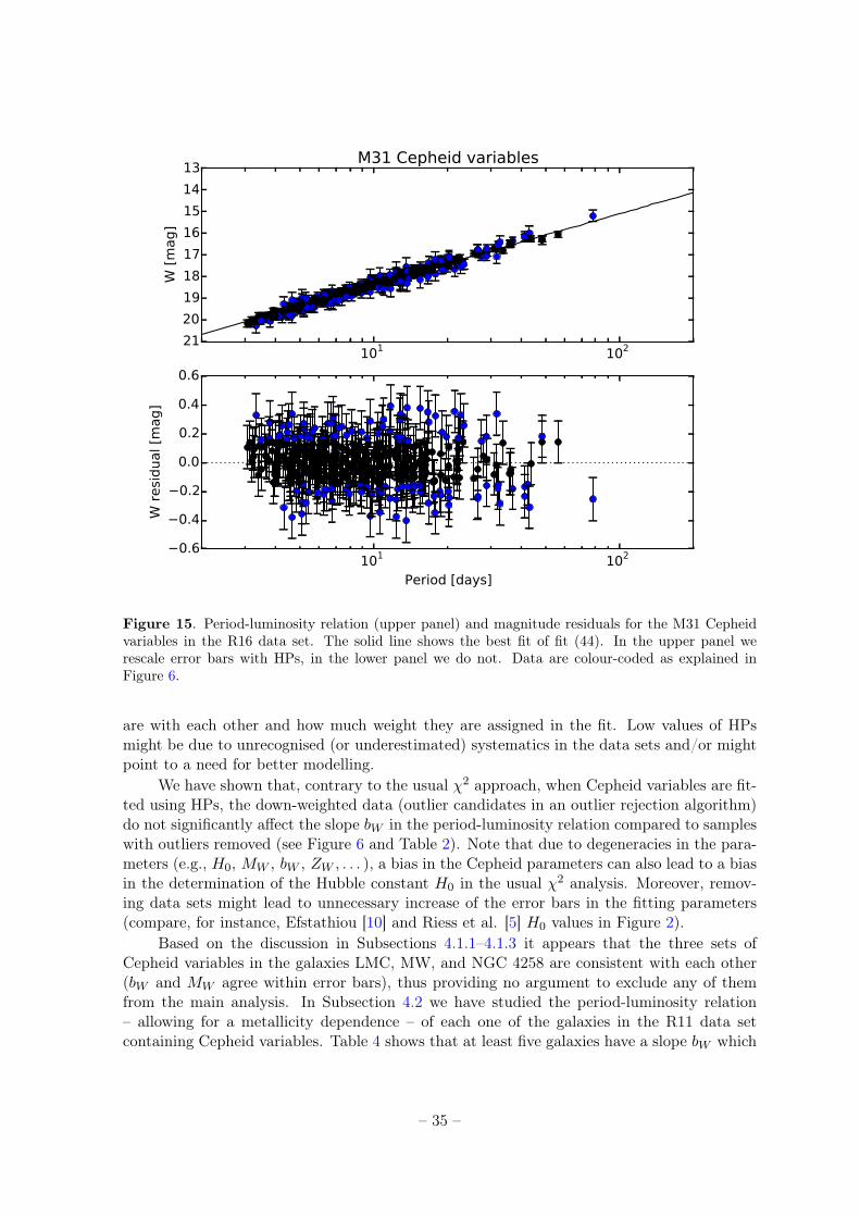
101 102
13
14
15
16
17
18
19
20
21
W [
mag]
M31 Cepheid variables
101 102
Period [days]
0.6
0.4
0.2
0.0
0.2
0.4
0.6
W r
esi
dual [m
ag]
Figure 15. Period-luminosity relation (upper panel) and magnitude residuals for the M31 Cepheidvariables in the R16 data set. The solid line shows the best fit of fit (44). In the upper panel werescale error bars with HPs, in the lower panel we do not. Data are colour-coded as explained inFigure 6.
are with each other and how much weight they are assigned in the fit. Low values of HPsmight be due to unrecognised (or underestimated) systematics in the data sets and/or mightpoint to a need for better modelling.
We have shown that, contrary to the usual χ2 approach, when Cepheid variables are fit-ted using HPs, the down-weighted data (outlier candidates in an outlier rejection algorithm)do not significantly affect the slope bW in the period-luminosity relation compared to sampleswith outliers removed (see Figure 6 and Table 2). Note that due to degeneracies in the para-meters (e.g., H0, MW , bW , ZW , . . . ), a bias in the Cepheid parameters can also lead to a biasin the determination of the Hubble constant H0 in the usual χ2 analysis. Moreover, remov-ing data sets might lead to unnecessary increase of the error bars in the fitting parameters(compare, for instance, Efstathiou [10] and Riess et al. [5] H0 values in Figure 2).
Based on the discussion in Subsections 4.1.1–4.1.3 it appears that the three sets ofCepheid variables in the galaxies LMC, MW, and NGC 4258 are consistent with each other(bW and MW agree within error bars), thus providing no argument to exclude any of themfrom the main analysis. In Subsection 4.2 we have studied the period-luminosity relation– allowing for a metallicity dependence – of each one of the galaxies in the R11 data setcontaining Cepheid variables. Table 4 shows that at least five galaxies have a slope bW which
– 35 –
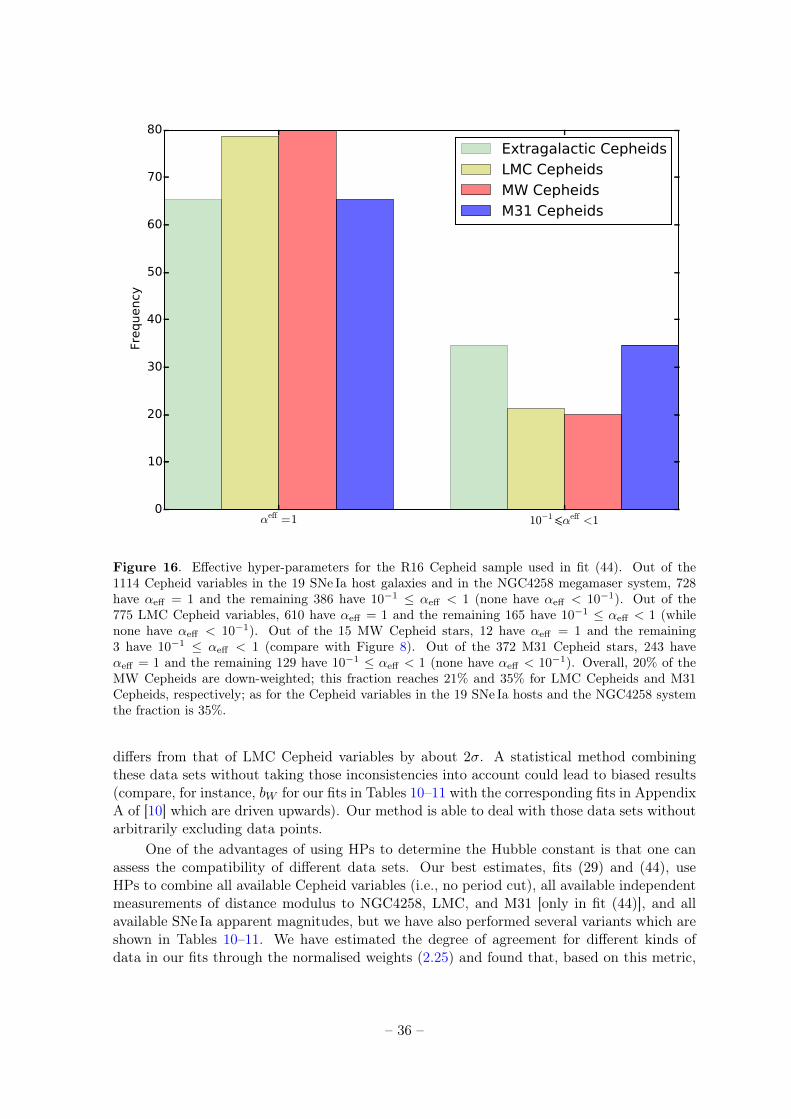
αeff =1 10−1 αeff <10
10
20
30
40
50
60
70
80Fr
equency
Extragalactic CepheidsLMC CepheidsMW CepheidsM31 Cepheids
Figure 16. Effective hyper-parameters for the R16 Cepheid sample used in fit (44). Out of the1114 Cepheid variables in the 19 SNe Ia host galaxies and in the NGC4258 megamaser system, 728have αeff = 1 and the remaining 386 have 10−1 ≤ αeff < 1 (none have αeff < 10−1). Out of the775 LMC Cepheid variables, 610 have αeff = 1 and the remaining 165 have 10−1 ≤ αeff < 1 (whilenone have αeff < 10−1). Out of the 15 MW Cepheid stars, 12 have αeff = 1 and the remaining3 have 10−1 ≤ αeff < 1 (compare with Figure 8). Out of the 372 M31 Cepheid stars, 243 haveαeff = 1 and the remaining 129 have 10−1 ≤ αeff < 1 (none have αeff < 10−1). Overall, 20% of theMW Cepheids are down-weighted; this fraction reaches 21% and 35% for LMC Cepheids and M31Cepheids, respectively; as for the Cepheid variables in the 19 SNe Ia hosts and the NGC4258 systemthe fraction is 35%.
differs from that of LMC Cepheid variables by about 2σ. A statistical method combiningthese data sets without taking those inconsistencies into account could lead to biased results(compare, for instance, bW for our fits in Tables 10–11 with the corresponding fits in AppendixA of [10] which are driven upwards). Our method is able to deal with those data sets withoutarbitrarily excluding data points.
One of the advantages of using HPs to determine the Hubble constant is that one canassess the compatibility of different data sets. Our best estimates, fits (29) and (44), useHPs to combine all available Cepheid variables (i.e., no period cut), all available independentmeasurements of distance modulus to NGC4258, LMC, and M31 [only in fit (44)], and allavailable SNe Ia apparent magnitudes, but we have also performed several variants which areshown in Tables 10–11. We have estimated the degree of agreement for different kinds ofdata in our fits through the normalised weights (2.25) and found that, based on this metric,
– 36 –
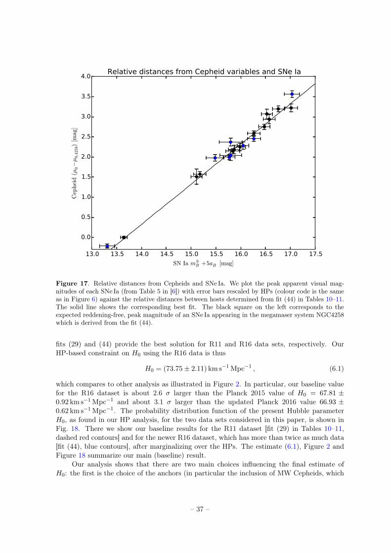
13.0 13.5 14.0 14.5 15.0 15.5 16.0 16.5 17.0 17.5
SN Ia m 0B +5aB [mag]
0.0
0.5
1.0
1.5
2.0
2.5
3.0
3.5
4.0C
ephei
d(µ
0−µ
0,4
258)
[mag
]Relative distances from Cepheid variables and SNe Ia
Figure 17. Relative distances from Cepheids and SNe Ia. We plot the peak apparent visual mag-nitudes of each SNe Ia (from Table 5 in [6]) with error bars rescaled by HPs (colour code is the sameas in Figure 6) against the relative distances between hosts determined from fit (44) in Tables 10–11.The solid line shows the corresponding best fit. The black square on the left corresponds to theexpected reddening-free, peak magnitude of an SNe Ia appearing in the megamaser system NGC4258which is derived from the fit (44).
fits (29) and (44) provide the best solution for R11 and R16 data sets, respectively. OurHP-based constraint on H0 using the R16 data is thus
H0 = (73.75± 2.11) km s−1 Mpc−1 , (6.1)
which compares to other analysis as illustrated in Figure 2. In particular, our baseline valuefor the R16 dataset is about 2.6 σ larger than the Planck 2015 value of H0 = 67.81 ±0.92 km s−1 Mpc−1 and about 3.1 σ larger than the updated Planck 2016 value 66.93 ±0.62 km s−1 Mpc−1. The probability distribution function of the present Hubble parameterH0, as found in our HP analysis, for the two data sets considered in this paper, is shown inFig. 18. There we show our baseline results for the R11 dataset [fit (29) in Tables 10–11,dashed red contours] and for the newer R16 dataset, which has more than twice as much data[fit (44), blue contours], after marginalizing over the HPs. The estimate (6.1), Figure 2 andFigure 18 summarize our main (baseline) result.
Our analysis shows that there are two main choices influencing the final estimate ofH0: the first is the choice of the anchors (in particular the inclusion of MW Cepheids, which
– 37 –
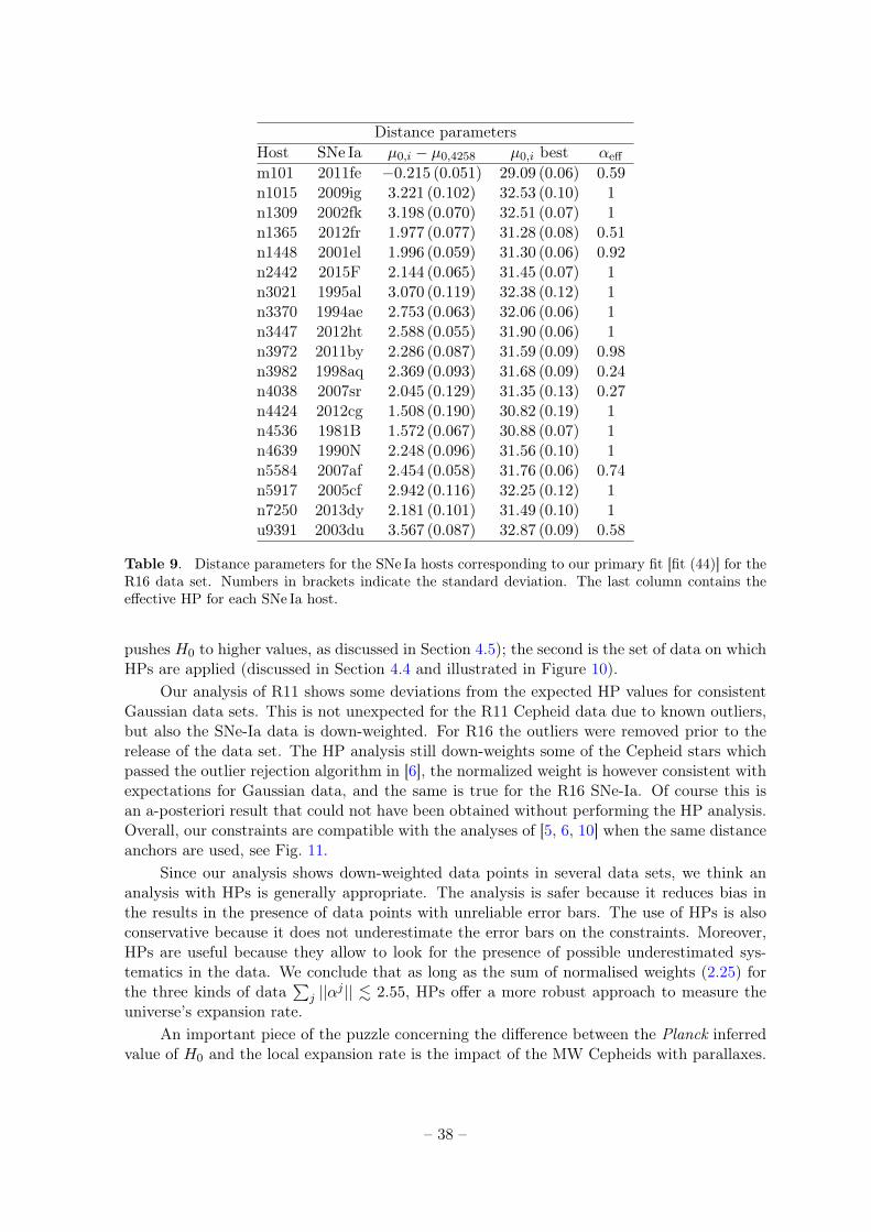
Distance parametersHost SNe Ia µ0,i − µ0,4258 µ0,i best αeff
m101 2011fe −0.215 (0.051) 29.09 (0.06) 0.59n1015 2009ig 3.221 (0.102) 32.53 (0.10) 1n1309 2002fk 3.198 (0.070) 32.51 (0.07) 1n1365 2012fr 1.977 (0.077) 31.28 (0.08) 0.51n1448 2001el 1.996 (0.059) 31.30 (0.06) 0.92n2442 2015F 2.144 (0.065) 31.45 (0.07) 1n3021 1995al 3.070 (0.119) 32.38 (0.12) 1n3370 1994ae 2.753 (0.063) 32.06 (0.06) 1n3447 2012ht 2.588 (0.055) 31.90 (0.06) 1n3972 2011by 2.286 (0.087) 31.59 (0.09) 0.98n3982 1998aq 2.369 (0.093) 31.68 (0.09) 0.24n4038 2007sr 2.045 (0.129) 31.35 (0.13) 0.27n4424 2012cg 1.508 (0.190) 30.82 (0.19) 1n4536 1981B 1.572 (0.067) 30.88 (0.07) 1n4639 1990N 2.248 (0.096) 31.56 (0.10) 1n5584 2007af 2.454 (0.058) 31.76 (0.06) 0.74n5917 2005cf 2.942 (0.116) 32.25 (0.12) 1n7250 2013dy 2.181 (0.101) 31.49 (0.10) 1u9391 2003du 3.567 (0.087) 32.87 (0.09) 0.58
Table 9. Distance parameters for the SNe Ia hosts corresponding to our primary fit [fit (44)] for theR16 data set. Numbers in brackets indicate the standard deviation. The last column contains theeffective HP for each SNe Ia host.
pushes H0 to higher values, as discussed in Section 4.5); the second is the set of data on whichHPs are applied (discussed in Section 4.4 and illustrated in Figure 10).
Our analysis of R11 shows some deviations from the expected HP values for consistentGaussian data sets. This is not unexpected for the R11 Cepheid data due to known outliers,but also the SNe-Ia data is down-weighted. For R16 the outliers were removed prior to therelease of the data set. The HP analysis still down-weights some of the Cepheid stars whichpassed the outlier rejection algorithm in [6], the normalized weight is however consistent withexpectations for Gaussian data, and the same is true for the R16 SNe-Ia. Of course this isan a-posteriori result that could not have been obtained without performing the HP analysis.Overall, our constraints are compatible with the analyses of [5, 6, 10] when the same distanceanchors are used, see Fig. 11.
Since our analysis shows down-weighted data points in several data sets, we think ananalysis with HPs is generally appropriate. The analysis is safer because it reduces bias inthe results in the presence of data points with unreliable error bars. The use of HPs is alsoconservative because it does not underestimate the error bars on the constraints. Moreover,HPs are useful because they allow to look for the presence of possible underestimated sys-tematics in the data. We conclude that as long as the sum of normalised weights (2.25) forthe three kinds of data
∑j ||αj || . 2.55, HPs offer a more robust approach to measure the
universe’s expansion rate.An important piece of the puzzle concerning the difference between the Planck inferred
value of H0 and the local expansion rate is the impact of the MW Cepheids with parallaxes.
– 38 –
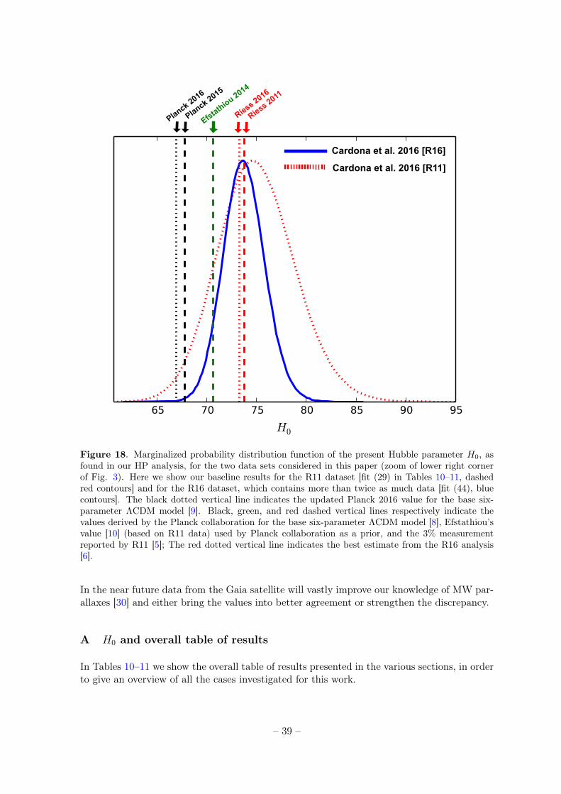
Cardona et al. 2016 [R16]
Cardona et al. 2016 [R11]
Planck 2016
Planck 2015
Efstathio
u 2014
Riess201
6
Riess201
1
Figure 18. Marginalized probability distribution function of the present Hubble parameter H0, asfound in our HP analysis, for the two data sets considered in this paper (zoom of lower right cornerof Fig. 3). Here we show our baseline results for the R11 dataset [fit (29) in Tables 10–11, dashedred contours] and for the R16 dataset, which contains more than twice as much data [fit (44), bluecontours]. The black dotted vertical line indicates the updated Planck 2016 value for the base six-parameter ΛCDM model [9]. Black, green, and red dashed vertical lines respectively indicate thevalues derived by the Planck collaboration for the base six-parameter ΛCDM model [8], Efstathiou’svalue [10] (based on R11 data) used by Planck collaboration as a prior, and the 3% measurementreported by R11 [5]; The red dotted vertical line indicates the best estimate from the R16 analysis[6].
In the near future data from the Gaia satellite will vastly improve our knowledge of MW par-allaxes [30] and either bring the values into better agreement or strengthen the discrepancy.
A H0 and overall table of results
In Tables 10–11 we show the overall table of results presented in the various sections, in orderto give an overview of all the cases investigated for this work.
– 39 –
Acknowledgments
We are very grateful to Adam Riess for assistance with the R16 data. We thank FilipeAbdalla for advice during the first stages of the project, at the SuperJedi Workshop 2013organized by Bruce Bassett. We further thank the programme ‘mobility in internationalresearch collaborations’ funded by the German excellence initiative for travel support. Partof the numerical work presented in this publication used the Baobab cluster of the Universityof Geneva. VP acknowledges the DFG TransRegio TRR33 grant on The Dark Universe.WC is supported by the Departamento Administrativo de Ciencia, Tecnología e Innovación(Colombia). MK acknowledges support by the Swiss NSF.
References
[1] W. L. Freedman, Determination of the Hubble Constant, 9612024.
[2] W. L. Freedman and B. F. Madore, The Hubble Constant, Ann. Rev. Astron. Astrophys. 48(2010) 673–710, [arXiv:1004.1856].
[3] W. Freedman, B. Madore, and B. Gibson, Final Results from the Hubble Space Telescope KeyProject to Measure the Hubble Constant, The Astrophysical Journal 553 (2001) 47–72.
[4] A. G. Riess et al., A Redetermination of the Hubble Constant with the Hubble Space Telescopefrom a Differential Distance Ladder, Astrophys. J. 699 (2009) 539–563, [arXiv:0905.0695].
[5] A. G. Riess, L. Macri, S. Casertano, H. Lampeitl, H. C. Ferguson, A. V. Filippenko, S. W. Jha,W. Li, and R. Chornock, A 3% Solution: Determination of the Hubble Constant with theHubble Space Telescope and Wide Field Camera 3, Astrophys. J. 730 (2011) 119,[arXiv:1103.2976]. [Erratum: Astrophys. J.732,129(2011)].
[6] A. G. Riess et al., A 2.4% Determination of the Local Value of the Hubble Constant, Astrophys.J. 826 (2016), no. 1 56, [arXiv:1604.01424].
[7] WMAP Collaboration, G. Hinshaw et al., Nine-Year Wilkinson Microwave Anisotropy Probe(WMAP) Observations: Cosmological Parameter Results, Astrophys. J. Suppl. 208 (2013) 19,[arXiv:1212.5226].
[8] Planck Collaboration, P. A. R. Ade et al., Planck 2015 results. XIII. Cosmological parameters,arXiv:1502.01589.
[9] Planck Collaboration, N. Aghanim et al., Planck intermediate results. XLVI. Reduction oflarge-scale systematic effects in HFI polarization maps and estimation of the reionizationoptical depth, arXiv:1605.02985.
[10] G. Efstathiou, H0 Revisited, Mon. Not. Roy. Astron. Soc. 440 (2014), no. 2 1138–1152,[arXiv:1311.3461].
[11] E. M. L. Humphreys, M. J. Reid, J. M. Moran, L. J. Greenhill, and A. L. Argon, Toward aNew Geometric Distance to the Active Galaxy NGC 4258. III. Final Results and the HubbleConstant, Astrophys. J. 775 (2013) 13, [arXiv:1307.6031].
[12] W. H. Press, Understanding data better with Bayesian and global statistical methods, inConference on Some Unsolved Problems in Astrophysics Princeton, New Jersey, April 27-29,1995, 1996. astro-ph/9604126.
[13] V. Marra, L. Amendola, I. Sawicki, and W. Valkenburg, Cosmic Variance and theMeasurement of the Local Hubble Parameter, Physical Review Letters 110 (jun, 2013) 241305.
[14] I. Ben-Dayan, R. Durrer, G. Marozzi, and D. J. Schwarz, The value of H0 in theinhomogeneous Universe, Phys. Rev. Lett. 112 (2014) 221301, [arXiv:1401.7973].
– 40 –
[15] A. E. Romano, Hubble trouble or Hubble bubble?, arXiv:1609.04081.
[16] C. Clarkson, O. Umeh, R. Maartens, and R. Durrer, What is the distance to the CMB?, JCAP1411 (2014), no. 11 036, [arXiv:1405.7860].
[17] C. Bonvin, C. Clarkson, R. Durrer, R. Maartens, and O. Umeh, Do we care about the distanceto the CMB? Clarifying the impact of second-order lensing, JCAP 1506 (2015), no. 06 050,[arXiv:1503.07831].
[18] S. Weinberg, Gravitation and Cosmology. John Wiley and Sons, New York, 1972.
[19] A. G. Riess et al., New Hubble Space Telescope Discoveries of Type Ia Supernovae at z>=1:Narrowing Constraints on the Early Behavior of Dark Energy, Astrophys. J. 659 (2007)98–121, [astro-ph/0611572].
[20] H. S. Leavitt and E. C. Pickering, Periods of 25 Variable Stars in the Small Magellanic Cloud.,Harvard College Observatory Circular 173 (Mar., 1912) 1–3.
[21] O. Lahav, S. L. Bridle, M. P. Hobson, A. N. Lasenby, and L. Sodre, Jr., Bayesian‘hyper-parameters’ approach to joint estimation: the hubble constant from cmb measurements,Mon. Not. Roy. Astron. Soc. 315 (2000) L45, [astro-ph/9912105].
[22] M. P. Hobson, S. L. Bridle, and O. Lahav, Combining cosmological datasets: hyperparametersand bayesian evidence, Mon. Not. Roy. Astron. Soc. 335 (2002) 377, [astro-ph/0203259].
[23] S. E. Persson, B. F. Madore, W. Krzemiński, W. L. Freedman, M. Roth, and D. C. Murphy,New Cepheid Period-Luminosity Relations for the Large Magellanic Cloud: 92 Near-InfraredLight Curves, The Astronomical Journal 128 (Nov., 2004) 2239–2264.
[24] K. M. Sebo, D. Rawson, J. Mould, B. F. Madore, M. E. Putman, J. A. Graham, W. L.Freedman, B. K. Gibson, and L. M. Germany, The Cepheid Period-Luminosity Relation in theLarge Magellanic Cloud, The Astrophysical Journal Supplement Series 142 (Sept., 2002) 71–78.
[25] F. van Leeuwen, M. W. Feast, P. A. Whitelock, and C. D. Laney, Cepheid Parallaxes and theHubble Constant, Mon. Not. Roy. Astron. Soc. 379 (2007) 723–737, [arXiv:0705.1592].
[26] J. Polshaw et al., A supernova distance to the anchor galaxy NGC 4258, Astron. Astrophys.580 (2015) L15, [arXiv:1509.00507].
[27] G. Pietrzynski et al., An eclipsing binary distance to the Large Magellanic Cloud accurate to 2per cent, Nature 495 (2013) 76–79, [arXiv:1303.2063].
[28] V. Bonvin et al., H0LiCOW V. New COSMOGRAIL time delays of HE0435-1223: H0 to 3.8%precision from strong lensing in a flat ΛCDM model, arXiv:1607.01790.
[29] Planck Collaboration, P. A. R. Ade, N. Aghanim, M. Arnaud, M. Ashdown, J. Aumont,C. Baccigalupi, A. J. Banday, R. B. Barreiro, N. Bartolo, and et al., Planck 2015 results. XIV.Dark energy and modified gravity, Astronomy and Astrophysics 594 (Sept., 2016) A14,[arXiv:1502.01590].
[30] S. Casertano, A. G. Riess, B. Bucciarelli, and M. G. Lattanzi, A test of Gaia Data Release 1parallaxes: implications for the local distance scale, ArXiv e-prints (Sept., 2016)[arXiv:1609.05175].
[31] L. Amendola, S. Appleby, A. Avgoustidis, D. Bacon, T. Baker, M. Baldi, N. Bartolo,A. Blanchard, C. Bonvin, S. Borgani, E. Branchini, C. Burrage, S. Camera, C. Carbone,L. Casarini, M. Cropper, C. de Rham, J. P. Dietrich, C. Di Porto, R. Durrer, A. Ealet, P. G.Ferreira, F. Finelli, J. Garcia-Bellido, T. Giannantonio, L. Guzzo, A. Heavens, L. Heisenberg,C. Heymans, H. Hoekstra, L. Hollenstein, R. Holmes, O. Horst, Z. Hwang, K. Jahnke, T. D.Kitching, T. Koivisto, M. Kunz, G. La Vacca, E. Linder, M. March, V. Marra, C. Martins,E. Majerotto, D. Markovic, D. Marsh, F. Marulli, R. Massey, Y. Mellier, F. Montanari, D. F.Mota, N. J. Nunes, W. Percival, V. Pettorino, C. Porciani, C. Quercellini, J. Read, M. Rinaldi,D. Sapone, I. Sawicki, R. Scaramella, C. Skordis, F. Simpson, A. Taylor, S. Thomas, R. Trotta,
– 41 –
L. Verde, F. Vernizzi, A. Vollmer, Y. Wang, J. Weller, and T. Zlosnik, Cosmology andFundamental Physics with the Euclid Satellite, ArXiv e-prints (June, 2016)[arXiv:1606.00180].
[32] J. L. Bernal, L. Verde, and A. G. Riess, The trouble with H0, JCAP 1610 (2016), no. 10 019,[arXiv:1607.05617].
[33] V. Pettorino, Testing modified gravity with Planck: The case of coupled dark energy, PhysicalReview D 88 (Sept., 2013) 063519, [arXiv:1305.7457].
– 42 –
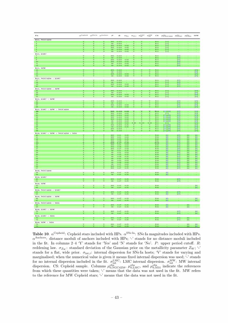
Fit αCepheid αSNe Ia αAnchors P R σZW σint,i σLMCint σMW
int CS µobs0,NGC4258 µobs
0,LMC µobs0,M31 MW
R11, NGC42581 Y Y Y 205 0.410 - V V - R11 [11] - - -2 Y Y Y 60 0.410 - V V - R11 [11] - - -3 Y Y Y 205 0.410 0.02 V V - R11 [11] - - -4 Y Y N 205 0.410 0.02 V V - R11 [11] - - -5 Y Y Y 60 0.410 0.02 V V - R11 [11] - - -6 Y Y N 60 0.410 0.02 V V - R11 [11] - - -
R11, LMC7 Y Y Y 205 0.410 - V V - R11 - [27] - -8 Y Y Y 60 0.410 - V V - R11 - [27] - -9 Y Y Y 205 0.410 0.02 V V - R11 - [27] - -10 Y Y N 205 0.410 0.02 V V - R11 - [27] - -11 Y Y Y 60 0.410 0.02 V V - R11 - [27] - -12 Y Y N 60 0.410 0.02 V V - R11 - [27] - -
R11, MW13 Y Y - 205 0.410 - V V V R11 - - - [25]14 Y Y - 60 0.410 - V V V R11 - - - [25]15 Y Y - 205 0.410 0.02 V V V R11 - - - [25]16 Y Y - 60 0.410 0.02 V V V R11 - - - [25]
R11, NGC4258 + LMC17 Y Y Y 205 0.410 - V V - R11 [11] [27] - -18 Y Y Y 60 0.410 - V V - R11 [11] [27] - -19 Y Y Y 205 0.410 0.02 V V - R11 [11] [27] - -20 Y Y Y 60 0.410 0.02 V V - R11 [11] [27] - -
R11, NGC4258 + MW21 Y Y Y 205 0.410 - V V V R11 [11] - - [25]22 Y Y Y 60 0.410 - V V V R11 [11] - - [25]23 Y Y Y 205 0.410 0.02 V V V R11 [11] - - [25]24 Y Y Y 60 0.410 0.02 V V V R11 [11] - - [25]
R11, LMC + MW25 Y Y Y 205 0.410 - V V V R11 - [27] - [25]26 Y Y Y 60 0.410 - V V V R11 - [27] - [25]27 Y Y Y 205 0.410 0.02 V V V R11 - [27] - [25]28 Y Y Y 60 0.410 0.02 V V V R11 - [27] - [25]
R11, LMC + MW + NGC425829 Y Y Y 205 0.410 0.02 V V V R11 [11],[26] [27] - [25]30 Y Y Y 205 0.410 0.02 V V V R11 [11] [27] - [25]31 Y N Y 205 0.410 0.02 V V V R11 [11],[26] [27] - [25]32 Y Y N 205 0.410 0.02 V V V R11 [11],[26] [27] - [25]33 Y N N 205 0.410 0.02 V V V R11 [11],[26] [27] - [25]34 Y Y Y 60 0.410 0.02 V V V R11 [11],[26] [27] - [25]35 Y N N 60 0.410 0.02 0.30 0.113 0.10 R11 [11] [27] - [25]36 Y Y Y 205 0.410 0.25 V V V R11 [11],[26] [27] - [25]37 Y Y Y 60 0.410 0.25 V V V R11 [11],[26] [27] - [25]38 Y Y Y 205 0.410 - V V V R11 [11],[26] [27] - [25]39 Y Y Y 60 0.410 - V V V R11 [11],[26] [27] - [25]
R16, LMC + MW + NGC4258 + M3140 Y Y Y 205 0.31 0.25 - - - R16 [6] [27] [6] [6]41 Y Y Y 205 0.31 0.02 - - - R16 [6] [27] [6] [6]42 Y Y Y 205 0.35 0.25 - - - R16 [6] [27] [6] [6]43 Y Y Y 205 0.39 0.25 - - - R16 [6] [27] [6] [6]44 Y Y Y 205 0.47 0.25 - - - R16 [6] [27] [6] [6]45 Y Y Y 205 0.35 0.02 - - - R16 [6] [27] [6] [6]46 Y Y Y 205 0.39 0.02 - - - R16 [6] [27] [6] [6]47 Y Y Y 205 0.47 0.02 - - - R16 [6] [27] [6] [6]48 Y Y Y 60 0.31 0.25 - - - R16 [6] [27] [6] [6]49 Y Y Y 60 0.31 0.02 - - - R16 [6] [27] [6] [6]50 Y Y Y 60 0.35 0.25 - - - R16 [6] [27] [6] [6]51 Y Y Y 60 0.39 0.25 - - - R16 [6] [27] [6] [6]52 Y Y Y 60 0.47 0.25 - - - R16 [6] [27] [6] [6]53 Y Y Y 60 0.35 0.02 - - - R16 [6] [27] [6] [6]54 Y Y Y 60 0.39 0.02 - - - R16 [6] [27] [6] [6]55 Y Y Y 60 0.47 0.02 - - - R16 [6] [27] [6] [6]56 N N N 205 0.47 0.25 - - - R16 [6] [27] [6] [6]57 N Y Y 205 0.47 0.25 - - - R16 [6] [27] [6] [6]
R16, NGC425858 Y Y Y 205 0.47 0.25 - - - R16 [6] - - -59 Y Y Y 60 0.47 0.25 - - - R16 [6] - - -
R16, LMC60 Y Y Y 205 0.47 0.25 - - - R16 - [27] - -61 Y Y Y 60 0.47 0.25 - - - R16 - [27] - -
R16, MW62 Y Y Y 205 0.47 0.25 - - - R16 - - - [6]63 Y Y Y 60 0.47 0.25 - - - R16 - - - [6]
R16, NGC4258 + LMC64 Y Y Y 205 0.47 0.25 - - - R16 [6] [27] - -65 Y Y Y 60 0.47 0.25 - - - R16 [6] [27] - -
R16, NGC4258 + MW66 Y Y Y 205 0.47 0.25 - - - R16 [6] - - [6]67 Y Y Y 60 0.47 0.25 - - - R16 [6] - - [6]
R16, NGC4258 + M3168 Y Y Y 205 0.47 0.25 - - - R16 [6] - [6] -69 Y Y Y 60 0.47 0.25 - - - R16 [6] - [6] -
R16, LMC + MW70 Y Y Y 205 0.47 0.25 - - - R16 - [27] - [6]71 Y Y Y 60 0.47 0.25 - - - R16 - [27] - [6]
R16, LMC + M3172 Y Y Y 205 0.47 0.25 - - - R16 - [27] [6] -73 Y Y Y 60 0.47 0.25 - - - R16 - [27] [6] -
R16, MW + M3174 Y Y Y 205 0.47 0.25 - - - R16 - - [6] [6]75 Y Y Y 60 0.47 0.25 - - - R16 - - [6] [6]
Table 10. αCepheid: Cepheid stars included with HPs. αSNe Ia: SNe Ia magnitudes included with HPs.αAnchors: distance moduli of anchors included with HPs; ‘-’ stands for no distance moduli includedin the fit. In columns 2–4 ‘Y’ stands for ‘Yes’ and ‘N’ stands for ‘No’. P : upper period cutoff. R:reddening law. σZW
: standard deviation of the Gaussian prior on the metallicity parameter ZW ; ‘-’stands for a flat, wide prior. σint,i: internal dispersion for SNe Ia hosts; ‘V’ stands for varying andmarginalised; when the numerical value is given it means fixed internal dispersion was used; ‘-’ standsfor no internal dispersion included in the fit. σLMC
int : LMC internal dispersion. σMWint : MW internal
dispersion. CS: Cepheid sample. Columns µobs0,NGC4258, µ
obs0,LMC, and µobs
0,M31 indicate the referencesfrom which these quantities were taken; ‘-’ means that the data was not used in the fit. MW refersto the reference for MW Cepheid stars; ‘-’ means that the data was not used in the fit.
– 43 –
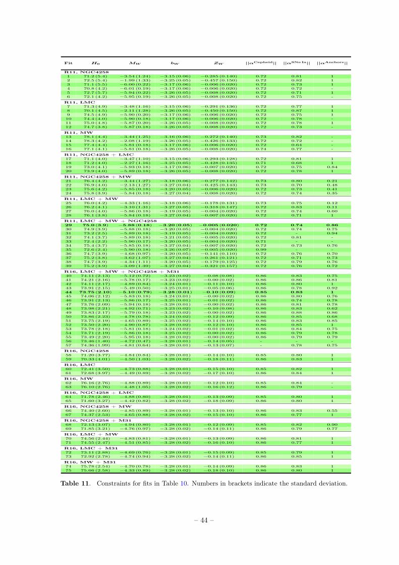
Fit H0 MW bW ZW ||αCepheid|| ||αSNe Ia|| ||αAnchors||
R11, NGC42581 71.2 (5.4) −3.54 (1.24) −3.15 (0.06) −0.285 (0.140) 0.72 0.81 12 72.5 (5.4) −1.99 (1.33) −3.25 (0.05) −0.457 (0.150) 0.72 0.82 13 71.1 (5.5) −6.00 (0.22) −3.17 (0.06) −0.006 (0.020) 0.72 0.73 14 70.8 (4.2) −6.01 (0.19) −3.17 (0.06) −0.006 (0.020) 0.72 0.72 -5 72.7 (5.7) −5.94 (0.22) −3.26 (0.05) −0.008 (0.020) 0.72 0.71 16 72.1 (4.2) −5.95 (0.19) −3.26 (0.05) −0.008 (0.020) 0.72 0.75 -
R11, LMC7 71.3 (4.9) −3.48 (1.16) −3.15 (0.06) −0.291 (0.136) 0.72 0.77 18 70.1 (4.5) −2.11 (1.28) −3.26 (0.05) −0.450 (0.150) 0.72 0.87 19 74.5 (4.9) −5.90 (0.20) −3.17 (0.06) −0.006 (0.020) 0.72 0.75 110 74.4 (4.0) −5.90 (0.18) −3.17 (0.06) −0.006 (0.020) 0.72 0.78 -11 75.0 (4.8) −5.87 (0.20) −3.26 (0.05) −0.008 (0.020) 0.72 0.78 112 74.7 (3.8) −5.87 (0.18) −3.26 (0.05) −0.008 (0.020) 0.72 0.73 -
R11, MW13 78.1 (4.4) −3.44 (1.25) −3.16 (0.06) −0.272 (0.140) 0.73 0.82 -14 78.3 (4.2) −2.08 (1.19) −3.26 (0.05) −0.426 (0.133) 0.72 0.72 -15 77.4 (4.4) −5.81 (0.18) −3.17 (0.06) −0.006 (0.020) 0.72 0.64 -16 77.1 (4.1) −5.81 (0.18) −3.26 (0.05) −0.008 (0.020) 0.74 0.77 -
R11, NGC4258 + LMC17 71.1 (4.0) −3.47 (1.10) −3.15 (0.06) −0.293 (0.128) 0.72 0.81 118 71.2 (4.0) −2.27 (1.16) −3.25 (0.05) −0.428 (0.135) 0.71 0.68 119 73.0 (4.1) −5.93 (0.18) −3.17 (0.06) −0.007 (0.020) 0.72 0.75 0.8420 73.9 (4.0) −5.89 (0.18) −3.26 (0.05) −0.008 (0.020) 0.72 0.78 1
R11, NGC4258 + MW21 76.4 (4.2) −3.44 (1.27) −3.18 (0.06) −0.277 (0.142) 0.73 0.80 0.2122 76.9 (4.0) −2.13 (1.27) −3.27 (0.04) −0.425 (0.143) 0.73 0.70 0.4823 75.6 (4.2) −5.85 (0.18) −3.20 (0.05) −0.006 (0.020) 0.72 0.73 0.4124 75.8 (3.9) −5.84 (0.18) −3.27 (0.04) −0.008 (0.020) 0.72 0.74 0.35
R11, LMC + MW25 76.0 (4.2) −4.33 (1.16) −3.18 (0.06) −0.178 (0.131) 0.73 0.75 0.1226 76.2 (4.1) −3.10 (1.31) −3.27 (0.05) −0.318 (0.147) 0.72 0.83 0.1127 76.0 (4.0) −5.86 (0.18) −3.19 (0.05) −0.004 (0.020) 0.72 0.74 0.6028 76.1 (3.8) −5.84 (0.18) −3.27 (0.04) −0.007 (0.020) 0.72 0.71 1
R11, LMC + MW + NGC425829 75.0 (3.9) −5.88 (0.18) −3.20 (0.05) −0.005 (0.020) 0.72 0.74 0.8630 74.9 (3.9) −5.88 (0.18) −3.20 (0.05) −0.004 (0.020) 0.72 0.74 0.7531 73.2 (2.5) −5.89 (0.18) −3.19 (0.05) −0.004 (0.020) 0.72 - 0.9432 74.1 (3.7) −5.89 (0.18) −3.21 (0.05) −0.005 (0.020) 0.72 0.81 -33 72.4 (2.2) −5.90 (0.17) −3.20 (0.05) −0.004 (0.020) 0.71 - -34 75.4 (3.7) −5.85 (0.18) −3.27 (0.04) −0.007 (0.020) 0.72 0.73 0.7635 72.6 (2.4) −5.90 (0.18) −3.26 (0.07) −0.005 (0.020) 0.99 - -36 74.7 (3.9) −4.68 (0.97) −3.20 (0.05) −0.141 (0.110) 0.72 0.76 0.7037 75.2 (3.8) −3.62 (1.07) −3.27 (0.04) −0.261 (0.121) 0.72 0.71 0.7338 74.7 (3.9) −4.34 (1.11) −3.20 (0.05) −0.179 (0.125) 0.72 0.79 0.7639 75.2 (3.9) −3.09 (1.39) −3.27 (0.04) −0.321 (0.157) 0.72 0.76 0.72
R16, LMC + MW + NGC4258 + M3140 74.11 (2.13) −5.12 (0.72) −3.23 (0.02) −0.08 (0.08) 0.86 0.83 0.7541 74.21 (2.16) −5.78 (0.17) −3.23 (0.02) −0.00 (0.02) 0.86 0.86 0.8142 74.11 (2.17) −4.89 (0.84) −3.24 (0.01) −0.11 (0.10) 0.86 0.80 143 73.91 (2.15) −5.49 (0.50) −3.25 (0.01) −0.05 (0.06) 0.86 0.78 0.9244 73.75 (2.10) −5.10 (0.79) −3.28 (0.01) −0.10 (0.09) 0.85 0.83 145 74.06 (2.12) −5.83 (0.18) −3.24 (0.01) −0.00 (0.02) 0.86 0.80 0.7646 73.91 (2.13) −5.86 (0.17) −3.25 (0.01) −0.01 (0.02) 0.86 0.74 0.7847 73.76 (2.09) −5.94 (0.18) −3.28 (0.01) −0.00 (0.02) 0.86 0.81 0.7848 73.98 (2.21) −4.92 (0.71) −3.23 (0.02) −0.10 (0.08) 0.86 0.83 0.6249 73.83 (2.17) −5.79 (0.18) −3.23 (0.02) −0.00 (0.02) 0.86 0.88 0.8650 73.86 (2.23) −4.78 (0.78) −3.24 (0.02) −0.12 (0.09) 0.86 0.85 0.6851 73.75 (2.19) −4.65 (0.89) −3.25 (0.02) −0.14 (0.10) 0.86 0.83 0.8552 73.50 (2.20) −4.90 (0.87) −3.28 (0.02) −0.12 (0.10) 0.86 0.85 153 73.78 (2.18) −5.81 (0.18) −3.24 (0.02) −0.01 (0.02) 0.86 0.84 0.7554 73.71 (2.19) −5.86 (0.18) −3.25 (0.02) −0.00 (0.02) 0.86 0.79 0.7855 73.49 (2.20) −5.95 (0.18) −3.28 (0.02) −0.00 (0.02) 0.86 0.79 0.7956 73.46 (1.40) −4.72 (0.47) −3.28 (0.01) −0.14 (0.05) - - -57 74.36 (1.99) −4.81 (0.64) −3.28 (0.01) −0.13 (0.07) - 0.78 0.75
R16, NGC425858 71.20 (3.77) −4.84 (0.84) −3.28 (0.01) −0.14 (0.10) 0.85 0.80 159 70.33 (4.01) −4.50 (1.03) −3.28 (0.02) −0.18 (0.11) 0.86 0.83 1
R16, LMC60 72.41 (3.50) −4.73 (0.88) −3.28 (0.01) −0.15 (0.10) 0.85 0.82 161 72.68 (3.97) −4.49 (0.89) −3.28 (0.02) −0.17 (0.10) 0.86 0.84 1
R16, MW62 76.16 (2.76) −4.88 (0.89) −3.28 (0.01) −0.12 (0.10) 0.85 0.84 -63 76.10 (2.76) −4.48 (1.05) −3.28 (0.02) −0.16 (0.12) 0.86 0.79 -
R16, NGC4258 + LMC64 71.78 (2.46) −4.88 (0.80) −3.28 (0.01) −0.13 (0.09) 0.85 0.80 165 71.60 (3.27) −4.42 (0.82) −3.28 (0.02) −0.18 (0.09) 0.86 0.80 1
R16, NGC4258 + MW66 74.40 (2.60) −4.85 (0.89) −3.28 (0.01) −0.13 (0.10) 0.86 0.83 0.5567 74.37 (2.53) −4.65 (0.88) −3.28 (0.02) −0.15 (0.10) 0.86 0.77 1
R16, NGC4258 + M3168 72.13 (3.07) −4.94 (0.80) −3.28 (0.01) −0.12 (0.09) 0.85 0.82 0.9069 71.85 (3.21) −4.76 (0.97) −3.28 (0.02) −0.14 (0.11) 0.86 0.79 0.77
R16, LMC + MW70 74.56 (2.44) −4.83 (0.81) −3.28 (0.01) −0.13 (0.09) 0.86 0.81 171 74.55 (2.47) −4.51 (0.85) −3.28 (0.02) −0.16 (0.10) 0.86 0.77 1
R16, LMC + M3172 73.11 (2.88) −4.69 (0.76) −3.28 (0.01) −0.15 (0.09) 0.85 0.79 173 72.92 (2.78) −4.74 (0.94) −3.28 (0.02) −0.14 (0.11) 0.86 0.85 1
R16, MW + M3174 75.78 (2.54) −4.70 (0.78) −3.28 (0.01) −0.14 (0.09) 0.86 0.83 175 75.66 (2.58) −4.33 (0.89) −3.28 (0.02) −0.18 (0.10) 0.86 0.80 1
Table 11. Constraints for fits in Table 10. Numbers in brackets indicate the standard deviation.
– 44 –