determinants of swaziland’s sugar export: a gravity model

International Journal of Economics and Finance; Vol. 8, No. 10; 2016

ISSN 1916-971X E-ISSN 1916-9728

Published by Canadian Center of Science and Education

71

Determinants of Swaziland’s Sugar Export: A Gravity Model

Approach

Sotja G. Dlamini1,2

, Abdi-Khalil Edriss1, Alexander R. Phiri

1 & Micah B. Masuku

2

1 Department of Agricultural and Applied Economics, Faculty of Development Studies, Lilongwe University of

Agriculture and Natural Resources, Lilongwe, Malawi

2 Department of Agricultural Economics and Management, Faculty of Agriculture, University of Swaziland,

Luyengo, Swaziland

Correspondence: Sotja G. Dlamini, Department of Agricultural Economics and Managent, Faculty of Agriculture,

University of Swaziland, Luyengo, Swaziland. E-mail: [email protected] or [email protected]

Received: August 6, 2016 Accepted: August 24, 2016 Online Published: September 25, 2016

doi:10.5539/ijef.v8n10p71 URL: http://dx.doi.org/10.5539/ijef.v8n10p71

Abstract

The sugar industry in Swaziland is the highest contributor to the government treasury through taxation, social

services and trade. The sugar industry also plays a crucial role in the Swaziland’s economy by influencing

economic growth and employment. Given the role of the Swaziland’s sugar industry, it is therefore important to

understand the influencing factors of the Swaziland sugar exports volumes to its major trading partners. The

study objective was to analyze the factors determining sugar export from Swaziland to her trading partners using

a gravity model approach. The study used panel dataset for the period 2001 to 2013. The results showed that

Swaziland’s GDP, importer’s GDP, importer’s land area and official common language had significant positive

effects on Swaziland’s sugar exports. The study further revealed that the creation of COMESA and EU trading

blocs had significant positive effects on the Swaziland’s sugar exports. This implies that the above-mentioned

factors have contributed to the sugar trade flows increase during the time period under study. On the other hand,

importer’s population, Swaziland openness and distance between Swaziland and her trading partner’s capital

cities had a significant negative effect on Swaziland’s sugar export flows. It is therefore recommended that

policies that lead to the exceptional advancement of the Swaziland and importer’s economy should be promoted

which will have an effects on the Swaziland GDP and importer’s GDP. Trading with less self-sufficient,

neighbouring countries and deepening the economic integration processes enhances Swaziland sugar exports

flows.

Keywords: exports, gravity model, panel data, sugar industry, Swaziland

1. Introduction

Swaziland’s sugar industry, which includes the growing of sugarcane and sugarcane manufacturing, contributes

about 18 percent to the Gross Domestic Product (GDP); employment in the sugarcane production takes up to 35

percent of the total wage employment, while sugarcane processing accounts for 18 percent of employment

opportunities in wage employment. The sugar industry is the highest contributor to the government treasury

through taxation, social services and trade, which includes exports and sugar related imports such as fuels,

chemical for agriculture and processing, transport and finance (Swaziland Sugar Association, 2012). There was

an enormous production expansion in the sugar industry since its existence in 1965 that resulted to an average

production of 214,305 tonnes per annum in the 1970s and 405,343 tonnes in the 1980s, to 480,154 tonnes in the

1990s and 587,621 tonnes by 2000. The average for the cropping year 2010/11 and 2012/13 was 687,000 tonnes.

The sugar production in the country from the 1970’s to current has shown an increase of about 321 percent and

this increase mainly arises from increase in acreage under sugarcane crop following expansion of the irrigation

projects that the country has invested on such as the Lower Usuthu Smallholder Irrigation Projects (LUSIP) and

Komati Downstream Development Project (KDDP). The Swaziland Sugar Association (SSA) is the only

institution that is responsible to market the Swaziland sugar and its by-products, except the by-products like

bagasse that is used by the sugar mills for firing boilers. The four main markets that the SSA served include;

European Union (EU), United States of America (USA), Southern African Customs Union (SACU) and the

regional/world market (Swaziland Sugar Association, 2013). The Southern African Customs Union (SACU),

ijef.ccsenet.org International Journal of Economics and Finance Vol. 8, No. 10; 2016

72

comprises; Swaziland, Botswana, South Africa, Lesotho and Namibia, constitutes the bulk of total sugar exports.

EU markets are the second largest, however prices per unit in this region are higher compared to the other Swazi

sugar exports market (Swaziland Sugar Association, 2011). Swaziland sugar sales to the EU and USA is though

preferential market access in terms of the ACP-EU Protocol on Sugar (SP) and Tariff Rate Quota (TRQ),

respectively and about 150 000 tonnes of sugar is sold to the EU with 120 000 tonnes sold under the Protocol on

Sugar and the remainder through Complementary Quantity (CQ). Total sales to the United States amount to

about 16 000 tonnes annually. Sales into the regional and world markets are mostly representative of left-overs

from sales into the main markets mentioned above. This market is typified by commonly low prices.

In 2006 the European Union (EU) reduced the reference price of sugar by 36 percent to €404.40 per tonne as part

of the sugar regime reform and hence that had led to the European sugar beet producers reducing domestic

production. The sugarcane producers in the African, Caribbean and Pacific (ACP) countries that had preferential

access to the EU also lost an estimated €462 million in export earnings due to the EU sugar reforms (Nyberg,

2006; OECD-FAO, 2011). From 1st October 2012, ACP sugar price guarantees were abolished and replaced by

the negotiated market-related price under the Interim Economic Partnership Agreement (IEPA). The negotiation

between certain Southern Africa Development Community (SADC) countries and the EU initialed in the end of

2007 is earmarked for the WTO-compatible Free Trade Agreement in order to maintain preferential market

access for Swaziland products and other ACP countries to the EU markets. The ACP sugar producers continued

to access duty-free quota of up to 3.5 million tonnes a year until 2015. After that, the only ACP sugarcane

producers that were able to access the duty-free quota were those that have sign WTO-compliant Economic

Partnership Agreements (EPA) with the EU (OECD-FAO, 2012). Given the role of the Swaziland sugar in the

economy and the challenges faced by the sugar industry in Swaziland, it is therefore important to understand the

main factors influencing the volume of Swaziland sugar exports to its major trading partners. This would be

important in guiding and designing of appropriate strategies and policies aimed at enhancing the country’s sugar

exports performance. The study objective was to analyze the factors determining sugar export volumes from

Swaziland to its trading partners using a gravity model approach. This study contributes by filling the knowledge

gap in literature since there is no empirical study that has employed the gravity model approach in understanding

the factors influencing the Swaziland sugar exports into its major trading countries.

2. Theoretical Framework

To analyse the determinants of Swaziland’s sugar exports volumes, the gravity trade model was used because it

has been applied extensively in the analysis of bilateral international trade flows for its considerable empirical

robustness and explanatory power. Tinbergen (1962) and Poyhonen (1963) were the pioneer of the gravity model

and they applied it to international trade literature firstly in the early 1960s. The basic gravity model in its

multiplicative form is represented as;

(1)

Where Xij is the flow of exports into country j from country i, Yi and Yj indicate the respective GDP for each

country while Dij is the geographical distance between the countries capital cities. The linear form of the gravity

model is as follows;

(2)

The generalized gravity model of trade as stated by Tinbergen (1962) suggested that one country is capable of

supplying exports to another country depends on its economic size and the magnitude of the importing country

market. Distance is used to specify the transportation cost for the goods between the two countries. The

coefficient signs of β1 and β2 are expected to be positive as GDP is interpreted as income while the coefficient

sign of β3 is expected to be negative, since the distance is a proxy for transport cost and the interpretation will

mean as the distance increases leads to the rise in the transport cost. However, early criticisms points out that the

gravity model lacks solid theoretical foundation. Anderson (1979) provided the first attempt of solid theoretical

justification of the gravity equation that was based on a demand function with a constant elasticity of substitution

(Armington preferences) where goods were country differentiated by origin. Bergstrand (1985, 1989) also

explored the theoretical determination of the bilateral trade in a series of papers by deriving the trade gravity

model based on monopolistic competition. Helpman and Krugman (1985) in justifying the theoretical derivation

of the gravity model they used the differentiated product framework with increasing return to scale. In the recent

literature many variables have been added to gravity model to reflect the factors determining trade flows

between trading partners like in Bergstrand (1989) encompass factor endowments and taste variables within the

Heckscher-Ohlin (H-O) model to explain the microeconomic foundations for the gravity equation. The trade

321

0

ijjiij DYYX

ijjiij DYYX lnlnlnln 3210


73

theories based on the H-O model justify the inclusion of only the core variables such as income, population and

distance. In the gravity equation additional variables can be incorporated to control for the differences in

geographical factors, historical ties and sets of dummy variables either restricting or facilitating trade between

countries pairs. Thus adding these variables into equation (1), the gravity model becomes;

ijuzm

ijijjijiij eeADNNYYX 654321

0

(3)

Where Xij is the value of exports flow into country j from country i, Yi and Yj indicate the respective GDP for

each country, Ni and Nj indicates the population for the exporter and importer, respectively while Dij is the

geographical distance between the countries capital cities. Aij represents other factors that could aid or impede

exports between countries, ezm

is a vector of dummy variables that test for specific effects, ijue is the error term

and the ’s are parameters of the model.

3. Methodology

3.1 Data Type and Sources

The data used in this study was annual panel data on Swaziland and her 24 major trading partners for the period

2001 to 2013. These countries were chosen based on the importance of trading partnership with Swaziland and

the availability of the required data. Panel data approach was chosen because it captures the relevant

relationships among variables over time and lowers the collinearity among the explanatory variables hence that

improves the estimates efficiency and controls the heterogeneity and dynamics of the unobservable individual

estimates (Baltagi, 2005). The sugar exports in USA dollars from Swaziland to her trading partners is the

dependent variable used in the analysis. The data were obtained from International Trade Centre database

(http://www.intracen.org). The independent variables used for the study included Gross Domestic Product (GDP),

population, exchange rate, geographical distance between the economic centres (i.e. capital cities) in Swaziland

and its trading partners, land area, openness to trade, language dummy, COMESA dummy, EU dummy. The

Gross Domestic Product (GDP) for Swaziland and its trading partners was measured in real terms at constant

2000 US$ to account for inflation. The data on GDPs were obtained from the World Bank, World

Development Indicators online database (http://www.databank.worldbank.org). Data on the total population of

the selected major trading partner countries were obtained from UN Population Division, World Population

Prospects, via the World Bank, World Development Indicators database (http://www.databank.worldbank.org).

The geographical land area of the trading partner was collected from the CEPII (Centre d’Etudes Prospectives et

d’Informations Internationales). The geographical distance between the economic centres (i.e. capital cities) of

Swaziland and her trading partners were measured in kilometres (km) and the data was obtained from

(http://distancecalculator.globefeed.com/country_Distance_calculator.asp). Data on real exchange rates and the

openness to trade variable that is computed as the total trade (the sum of exports and imports) of a nation along

with the world economy divided by its real GDP. Both data were obtained from International Financial Statistics

(IFS) database that was developed by International Monetary Fund (IMF) (http://www.imf.org/external/data.htm).

The dummy variable for COMESA and EU trade agreements were obtained from COMESA Community’s

website (http://www.comesa.int ) and the EU’s country list website (http://www.eucountrylist.com ), respectively.

The official language of Swaziland and its trading partner’s data were sourced from the Central Intelligence

Agency (CIA) World Fact Book.

3.2 Model Specification

The main objective of this study was to analyze the factors that determine the sugar export from Swaziland to its

trading partners using a gravity model approach. The gravity model of trade was used because it has been

applied extensively in the analysis of bilateral international trade flows. The gravity equation postulates that the

size of bilateral trade flows between two countries is proportional to the economic sizes of the two countries,

proxied by GDP, and inversely proportional to their economic distance usually represented by the physical

distance between them. Empirical works by Martinez-Zarzoso and Nowak-Lehman (2003) conforming the

general form of the gravity model that the exports volume between two countries is not only influenced by their

economic masses proxied by GDPs and distance between them, but also by population and a collection of

dummies that are included in the gravity equation to control for the differences in geographical factors, historical

ties and the trade agreements between the nations that trade. Hence, for this study the dummy variables such as

common official language, the trading partner being an EU member state or COMESA member state and that the

trading partner was colonized by the British same as Swaziland were added to the gravity equation to capture

other factors that may possible influence the sugar exports. Other important variables such as real exchange rate,

the country openness to trade and the trading partner country area size were added to the gravity equation which


74

that may explain the impact of various policy issues on the sugar exports. Thus, by introducing these variables,

the augmented gravity model becomes;

ijjtjtitijtijtjtitjtitijt LangAreaOpenOpenRERDNNYYX 100987654321

(4)

For estimation purposes, the gravity model is used in its log-linear form, therefore, Equation (4) is written in its

natural logarithms as;

ijtijtjtitjtitijt RERDNNYYX lnlnlnlnlnlnln 6543210

EULangAreaOpenOpen ijjtjtit 1110987 lnlnln

ijtij COMESACol 1312

(5)

Where:

i indicates the exporter (Swaziland), j are the trading partners (importer) and t is period under consideration, i.e.

2001 to 2013,

Xijt : is the value of Swaziland sugar exports (in US dollars) to country j;

Yi and Yj: are the GDPs of the exporter (Swaziland) and importer (trading partner) at time t, respectively;

𝑁𝑖 and 𝑁𝑗: are the population size of Swaziland and country j at time t, respectively;

Dijt: is the geographical distance in kilometres between Swaziland’s capital city (Mbabane) and trading partner’s

capital city;

RERijt: is the bilateral real exchange rate between Swaziland and the trading partner;

Openi and Openj: is the openness to trade exhibits of Swaziland and country j at time t, respectively;

Areaj: is the geographical land that the trading partner covers;

Langij: is a dummy variable to capture official language as English, taking value of 1 if the trading partner speaks

English, and zero otherwise;

Colij: is a dummy variable taking a value of one if the trading partner share a common colonial history with

Swaziland, and zero otherwise;

EU: European country dummy (European country coded one and zero otherwise);

COMESA: COMESA dummy variable (if the trading partner is a member of COMESA coded one and zero

otherwise);

𝜇𝑖𝑗t: is the error term.

All the variables are expressed in natural logarithms except dummy variables.

According to theory, the coefficient of the GDPs of the home (Swaziland) and host (trading partners) countries

are used as proxy for the economic sizes of the countries and it is expected that an importing county’s GDP plays

a significant role in determining the trade flows originating from the exporting country (Frankel,1997). The

importing countries GDP is treated as customer income, determined the goods demand originating from the

exporting country. The GDP of the exporting country helps in ascertaining productive capacity of exporting

country. The gravity model hypothesize that GDP for the exporting country influences the trade flows of goods

originating from the exporting country. Thus, as GDP of any two or more trading countries increases, trade flows

will also increase. Therefore the coefficients of GDPs are expected to be positive. The coefficient of the

population is used to measure the impact of Swaziland’s and that of her trading partner’s degree of

self-sufficiency and absorption effect. An exporting country with a huge population size is expected to produce

and export more due to economies of scale resulting from ‘cheap’ labour. However, it can also export less due to

higher domestic absorption effect of larger population size. Hence, the coefficient of exporter’s population can

be positively or negatively signed. On other hand, an importing country with a huge population size is indicative

of potentially larger market size and is expected to import more. Hence, the coefficient of the partners’

population is expected to be positive.

The coefficient of distance is used to capture the proxy for the trade cost between countries. Distance is a trading

resistance factor that represents trade barriers such as transportation costs, time-related costs and cultural costs.

ijtu

ij COMESAColEU 131211


75

The greater the geographic distance between pairs of trading partners, the higher will be the associated

transaction costs. This will increase products’ prices and subsequently erode their competitiveness and gains

from trade. This reduces the extent to which they trade with each other. The estimated coefficient of distance is

anticipated to have a negative sign. The coefficient of bilateral real exchange rate is incorporated as a proxy for

the relative price of foreign goods in terms of domestic goods. The real bilateral exchange rate measures the

international competitiveness of goods produced domestically. An increase in the real exchange (or real

depreciation) means that it takes fewer units of foreign currency to buy one unit of domestic currency. This

makes domestic goods relatively cheaper, leading to an increase in exports due to higher foreign demand. The

decrease or appreciation of the real exchange rate decreases in an economy is associated with loses in

competiveness because more units of foreign currency to buy one unit of domestic currency will be required.

This raises the price of exported goods and lowers that of imported goods, leading to increase in imports due to

higher domestic demand. Thus, coefficient of exchange rate is expected to be negative since it affect exports.

The coefficient of openness to trade reflects an economy’s openness to the flow of goods and services from

around the world. The citizen’s ability to interact freely as buyer or seller in the international marketplace. The

mostly used trade restrictions are in the form of tariffs, export taxes, trade quotas, or outright trade bans. Trade

restrictions also appear in the form of regulatory barriers. The degree to which government hinders the free flow

of foreign goods and services has a direct bearing on the ability of individuals to pursue their economic goals and

maximize their productivity and well-being. Tariffs, for example, directly increase the prices that local

consumers pay for foreign imports, but they also distort production incentives for local producers, causing them

to produce either a good in which they lack a comparative advantage or more of a protected good than is

economically efficient. This impedes overall economic efficiency and growth. Thus, the more open an economy

is, as indicated by high trade freedom rating, the more it is expected to trade with other economies. Hence, it is

expected that the coefficient will be positive.

The dummy variable of language is being used as a proxy of historical and cultural links, which are particularly

important at reducing the cost of unfamiliarity in international trade. Sharing similar culture not only reflects the

high propensity of the people in two countries to consume similar goods but indicates a lower cost of doing

business for firms from one country in another. Thus, sharing common language helps to facilitate and expedite

trade negotiations, reduce transaction costs and increase the level of trade between both countries (Melitz &

Toubal, 2012). Thus, its coefficient is expected to be positive. The colonial dummy variable which was also

added to capture the influence of colonial masters on bilateral trade flows among the trading partners. It is

expected that countries which were colonised by the same country will have more trading opportunities and

hence the coefficient is expected to have a positive sign. Land area size supplements economic size variables

since it incorporates information about natural resources in the model. This variable is used as a proxy for

resource endowments. Larger countries have more diversified production and tend to be more self-sufficient. It is

normally expected to be negatively related to trade. The formation of economic agreement increases the market

size of member countries and attracts non-member countries to transact business in the region. Regional trade

blocs and preferential trade agreements are found to be trade enhancing in many empirical studies. In this study,

EU and COMESA are dummy variables introduced to control for the effects of trade agreements between

Swaziland and its trading partners. It is expected that the coefficients will be positive.

3.3 Analytical Technique

The augmented gravity model equation (5) was estimated using the three models that can be applied in panel

data estimation. These models are pooled ordinary least squares (POLS), fixed effects (FE) and random effects

(RE) approaches. Since the regression models include individual effects, it is important to identify whether they

are treated as random or fixed effects. A random effects model can be more appropriate when estimating the

trade flows between randomly selected samples of trading partners from a large population, while the fixed

effects model is better when estimating the trade flows between an ex ante predetermined selection of countries

(Egger, 2000; Eita & Jordaan, 2007). This study objective is to analyse the determinants of Swaziland sugar

exports to its 24 major trading partners, thus fixed effect model will be more appropriate model than the random

effect model. The study also applies the Hausman test statistic to check further if the fixed effects model is more

efficient than the random effects model. Therefore, if the null hypothesis of no correlation between the individual

effects and the regressors is rejected, it will mean that the fixed effects model is better than the random effects

model.

The main problem with a fixed effects model is that it does not allow for estimation of coefficients of

time-invariant variables such as distance (Baltagi, 2001; Wooldridge, 2002). To solve this problem a method

such as the Least Squares Dummy Variables (LSDV) have been developed in empirical literature (Greene, 2013).


76

The LSDV estimator provides the country-specific fixed effects estimation, which is the second step of the

two-stage regression procedure where it was separated from the fixed effects effect estimation. Unlike the within

fixed effect method, it works for all time-invariant variables in the model. The model introduces heterogeneity,

but unlike the fixed effects model it minimizes the loss of degree of freedom and presupposes a specific

distribution (i.e., each country differs in its error term) (Eita & Jordaan, 2007).

This is signified as follows:

𝐼𝐸𝑖𝑗 = 𝛾0 + 𝛾1𝐷𝑖𝑗 + 𝛾2𝐿𝑎𝑛𝑔ij + 𝛾3COMESA + 𝛾4 EU + 𝛾5Colij + 𝜇𝑖𝑗 (6)

Where; 𝐼𝐸𝑖𝑗 stands for the individual effects, other variables are denoted as before. With the random effects

model (REM), distinctive trade flows are estimated from a larger population amongst randomly drawn samples

of trading partners and no individual specific effects are reflected on its estimated coefficients (Gujarati, 2009).

3.4 Univariate Characteristics of Variables

In view of the nature of the dataset employed in this study, it is imperative to start by analysing the univariate

characteristics of the data that enter the gravity model using the panel unit root tests. If all variables are

stationary, then the traditional estimation methods can be used to estimate the relationship between the variables.

If the variables are non-stationary a test for cointegration should be performed (Hadri, 2000). Levin Lin Chu

(LLC) and Im, Pesaran and Shin (IPS) panel unit root tests was employed to investigate the stationarity of the

panel data, following the procedure described by Baltagi (2008).

4. Results and Discussion

4.1 Stationarity Tests

The panel unit root tests using Levin Lin Chu (LLC) and Im, Pesaran and Shin (IPS) panel unit root tests was

done on all the variables by means of the test regression, encompassing only individual intercepts or constants

with trend specification. The panel unit root test was not applied to dummy variables because they are fixed and

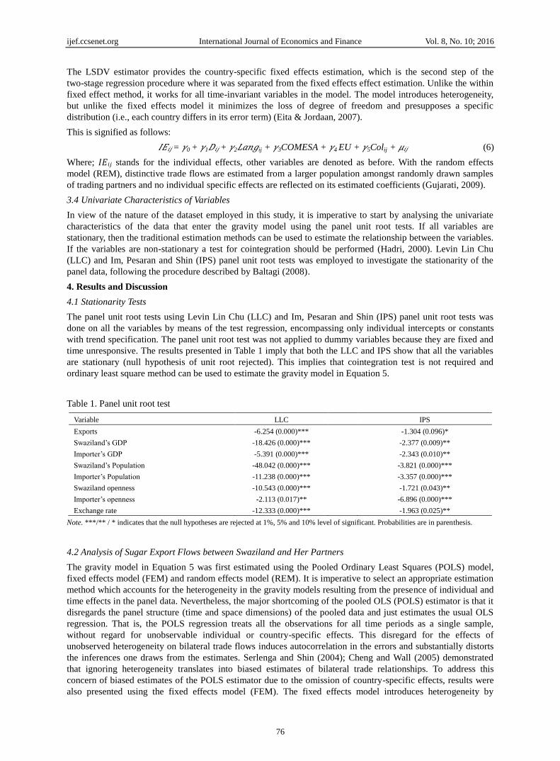
time unresponsive. The results presented in Table 1 imply that both the LLC and IPS show that all the variables

are stationary (null hypothesis of unit root rejected). This implies that cointegration test is not required and

ordinary least square method can be used to estimate the gravity model in Equation 5.

Table 1. Panel unit root test

Variable LLC IPS

Exports

Swaziland’s GDP

Importer’s GDP

Swaziland’s Population

Importer’s Population

Swaziland openness

Importer’s openness

Exchange rate

-6.254 (0.000)***

-18.426 (0.000)***

-5.391 (0.000)***

-48.042 (0.000)***

-11.238 (0.000)***

-10.543 (0.000)***

-2.113 (0.017)**

-12.333 (0.000)***

-1.304 (0.096)*

-2.377 (0.009)**

-2.343 (0.010)**

-3.821 (0.000)***

-3.357 (0.000)***

-1.721 (0.043)**

-6.896 (0.000)***

-1.963 (0.025)**

Note. ***/** / * indicates that the null hypotheses are rejected at 1%, 5% and 10% level of significant. Probabilities are in parenthesis.

4.2 Analysis of Sugar Export Flows between Swaziland and Her Partners

The gravity model in Equation 5 was first estimated using the Pooled Ordinary Least Squares (POLS) model,

fixed effects model (FEM) and random effects model (REM). It is imperative to select an appropriate estimation

method which accounts for the heterogeneity in the gravity models resulting from the presence of individual and

time effects in the panel data. Nevertheless, the major shortcoming of the pooled OLS (POLS) estimator is that it

disregards the panel structure (time and space dimensions) of the pooled data and just estimates the usual OLS

regression. That is, the POLS regression treats all the observations for all time periods as a single sample,

without regard for unobservable individual or country-specific effects. This disregard for the effects of

unobserved heterogeneity on bilateral trade flows induces autocorrelation in the errors and substantially distorts

the inferences one draws from the estimates. Serlenga and Shin (2004); Cheng and Wall (2005) demonstrated

that ignoring heterogeneity translates into biased estimates of bilateral trade relationships. To address this

concern of biased estimates of the POLS estimator due to the omission of country-specific effects, results were

also presented using the fixed effects model (FEM). The fixed effects model introduces heterogeneity by


77

estimating country specific effects. It also allows the intercept and other parameters to vary across trading

partners. The F-test statistic was performed to test the ability to pool data and the results in Table 2 indicates that

the null hypothesis of equality of individual effects was rejected, which implies that the model with individual

effects is better than the pooled model.

Hausman test was then applied to check efficient model between the fixed effects model and the random effects

model. This would be true if the null hypothesis of no correlation between the regressors and the individual

effects. Failure to reject the null hypothesis implies that the random effects model will be preferred. Fixed effects

model will be appropriate if the null hypothesis is rejected. The results in Table 2 reveal that the Hausman

specification test rejects the null hypothesis and that means the country specific effects are correlated with

regressors. This suggests that the fixed effects model is preferred. Since the fixed effect model is appropriate, the

interpretation of the results was centred on the fixed effects model.

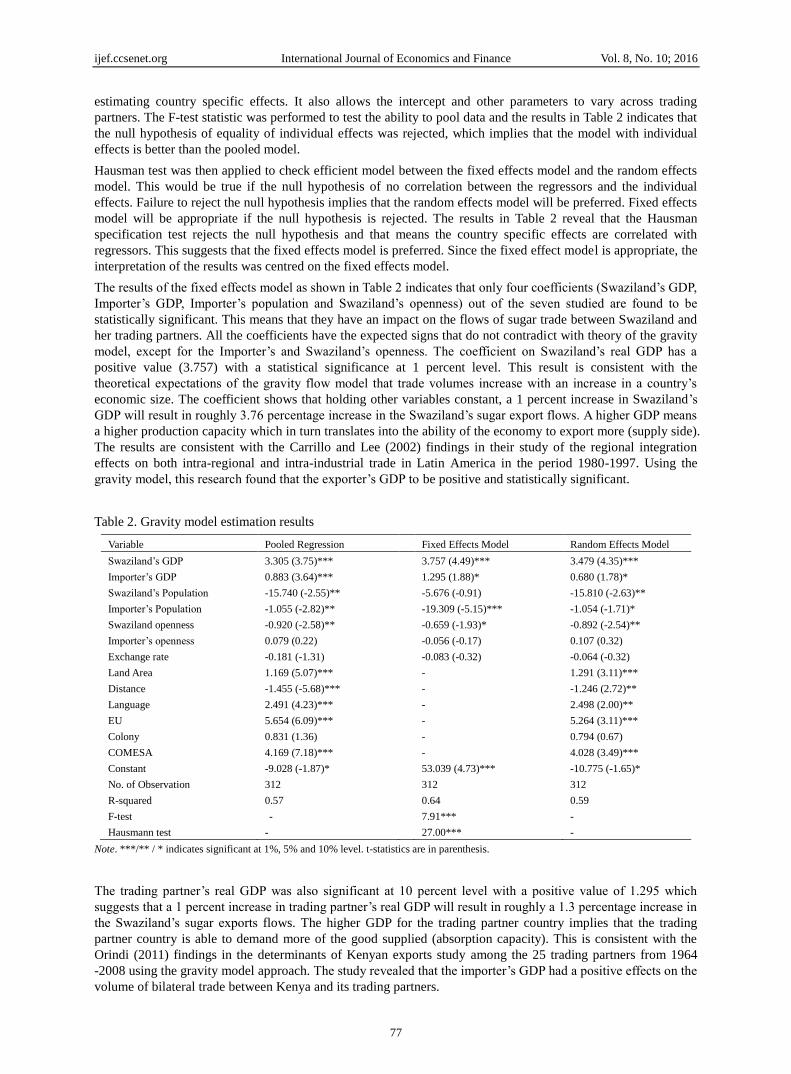
The results of the fixed effects model as shown in Table 2 indicates that only four coefficients (Swaziland’s GDP,

Importer’s GDP, Importer’s population and Swaziland’s openness) out of the seven studied are found to be

statistically significant. This means that they have an impact on the flows of sugar trade between Swaziland and

her trading partners. All the coefficients have the expected signs that do not contradict with theory of the gravity

model, except for the Importer’s and Swaziland’s openness. The coefficient on Swaziland’s real GDP has a

positive value (3.757) with a statistical significance at 1 percent level. This result is consistent with the

theoretical expectations of the gravity flow model that trade volumes increase with an increase in a country’s

economic size. The coefficient shows that holding other variables constant, a 1 percent increase in Swaziland’s

GDP will result in roughly 3.76 percentage increase in the Swaziland’s sugar export flows. A higher GDP means

a higher production capacity which in turn translates into the ability of the economy to export more (supply side).

The results are consistent with the Carrillo and Lee (2002) findings in their study of the regional integration

effects on both intra-regional and intra-industrial trade in Latin America in the period 1980-1997. Using the

gravity model, this research found that the exporter’s GDP to be positive and statistically significant.

Table 2. Gravity model estimation results

Variable Pooled Regression Fixed Effects Model Random Effects Model

Swaziland’s GDP

Importer’s GDP

Swaziland’s Population

Importer’s Population

Swaziland openness

Importer’s openness

Exchange rate

Land Area

Distance

Language

EU

Colony

COMESA

Constant

No. of Observation

R-squared

F-test

Hausmann test

3.305 (3.75)***

0.883 (3.64)***

-15.740 (-2.55)**

-1.055 (-2.82)**

-0.920 (-2.58)**

0.079 (0.22)

-0.181 (-1.31)

1.169 (5.07)***

-1.455 (-5.68)***

2.491 (4.23)***

5.654 (6.09)***

0.831 (1.36)

4.169 (7.18)***

-9.028 (-1.87)*

312

0.57

-

-

3.757 (4.49)***

1.295 (1.88)*

-5.676 (-0.91)

-19.309 (-5.15)***

-0.659 (-1.93)*

-0.056 (-0.17)

-0.083 (-0.32)

-

-

-

-

-

-

53.039 (4.73)***

312

0.64

7.91***

27.00***

3.479 (4.35)***

0.680 (1.78)*

-15.810 (-2.63)**

-1.054 (-1.71)*

-0.892 (-2.54)**

0.107 (0.32)

-0.064 (-0.32)

1.291 (3.11)***

-1.246 (2.72)**

2.498 (2.00)**

5.264 (3.11)***

0.794 (0.67)

4.028 (3.49)***

-10.775 (-1.65)*

312

0.59

-

-

Note. ***/** / * indicates significant at 1%, 5% and 10% level. t-statistics are in parenthesis.

The trading partner’s real GDP was also significant at 10 percent level with a positive value of 1.295 which

suggests that a 1 percent increase in trading partner’s real GDP will result in roughly a 1.3 percentage increase in

the Swaziland’s sugar exports flows. The higher GDP for the trading partner country implies that the trading

partner country is able to demand more of the good supplied (absorption capacity). This is consistent with the

Orindi (2011) findings in the determinants of Kenyan exports study among the 25 trading partners from 1964

-2008 using the gravity model approach. The study revealed that the importer’s GDP had a positive effects on the

volume of bilateral trade between Kenya and its trading partners.


78

The coefficient of the Swaziland’s population was negative and was not statistically significant. This means that

it cannot be considered as an explanatory variable for the demand for Swaziland sugar exports. Importer’s

population coefficient with a negative value of 19.309 was statistically significant at 1 percent level. These

results reveal that an increase in the trading partners’ population by 1 percent leads to 19.3 percent decline in the

Swaziland sugar exports. Ideally, one would argue that the population growth in an importing country creates

more market for the exporting country but in the case of Swaziland, it is the contrary. The negative relationship

between trade flow and trade partners’ population can be attributed to a condition referred to as exporter

substitution effect. This implies that the trading partner’s population leads to the expansion of domestic markets,

thus creating a greater magnitude of self-sustenance and, as a consequence, there will be no exigency to trade

between them. These results are in conformity with the expected theories and correspond favourably to those

computed by Giorgio (2004); Eita and Joordan (2007); amongst others that found that the bigger the population

of the trading partner, the larger the production for the domestic market.

The results further revealed that the coefficient of Swaziland openness has unexpected negative sign value

(-0.659), that was statistically significant at 10 percent level. This implies that Swaziland sugar exports would

considerably decrease together with Swaziland trade barriers’ liberalisation. In addition, the regression’s result

suggests that a 1 percent increase in the Swaziland trade openness leads to a decrease by 0.66 percent of the

Swaziland sugar exports. The importer’s openness variable does not have the expected positive sign, but was

found to be statistically insignificant. This means that this variable seems not to have an effect on the flows of

trade between Swaziland and her trading partner countries. Although, the expected negative sign of the

coefficient of the real exchange rate, it was not statistically significant. This meant that it cannot be considered as

an explanatory variable for the demand for Swaziland’s sugar exports.

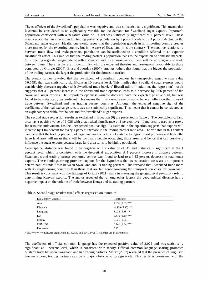
The second stage regression results as explained in Equation (6) are presented in Table 3. The coefficient of land

area has a positive value of 1.036 with a statistical significance at 1 percent level. Land area is used as a proxy

for resource endowment, has the unexpected positive sign. Its estimate in the equation suggests that exports will

increase by 1.04 percent for every 1 percent increase in the trading partner land area. The variable in this content

can mean that the trading partner had large land area which is not suitable for agricultural purposes and hence the

large land area will mean there will be too many people occupying those areas and hence that can positively

influence the sugar exports because large land area turns to be highly populated.

Geographical distance was found to be negative with a value of -1.119 and statistically significant at the 1

percent level, which is consistent with the theoretical expectation. A 1 percent increase in distance between

Swaziland’s and trading partner economic centres was found to lead to a 1.12 percent decrease in total sugar

exports. These findings strong provides support for the hypothesis that transportation costs are an important

determinant of trade flows between Swaziland and its trading partners. This revealed that Swaziland trade more

with its neighbouring countries than those that are far, hence lowering the transportation costs for Swaziland.

This result is consistent with the findings of Orindi (2011) study in assessing the geographical proximity role in

determining Kenyan exports. The author revealed that among other factors the geographical distance had a

negative impact on the volume of trade between Kenya and its trading partners

Table 3. Second stage results: fixed effects regressed on dummies

Explanatory Variable Coefficient

Area

Distance

Language

EU

Colony

COMESA

R-squared

1.036 (8.55)***

-1.119 (5.33)***

3.022 (5.38)***

6.410 (9.19)***

0.021 (0.04)

3.141 (5.24)***

0.42

Note. ***/** / * indicates significant at 1%, 5% and 10% level. T-statistics are in parenthesis.

The coefficient of official common language has the expected positive value of 3.022 and was statistically

significant at 1 percent level, which is consistent with theory. Official common language sharing promotes

bilateral trade between Swaziland and her trading partners. Melitz (2007) revealed that the presence of linguistic

barriers among trading partners can be a major obstacle to foreign trade. This result is consistent with the


79

previous findings of Achay (2006), Eita and Jordaan (2007). These authors in their empirical studies revealed

that there is a strong positive effect of the language variable that made them to conclude that historical, cultural

and colonial ties had a significant impact on the pattern of trade in their study samples.

The coefficient of the COMESA dummy had the expected positive value of 3.141 that was significant at 1

percent level. The COMESA dummy variable suggests that Swaziland’s trades more with COMESA members,

since they have deep influence on the mutual trade between member countries. This result may be due to the

many countries in COMESA, which provide a trade opportunity with Swaziland. These COMESA member

states provide ready import and export market for Swaziland, hence boosting her trade. Therefore, if Swaziland’s

trade partners belong to COMESA, Swaziland’s sugar exports with those countries would be about three times as

great as trade partners with a non-COMESA country. This result is very similar to the results obtained by Frankel

(1997) and Chan-Hyun (2005). Such findings imply that membership to regional trade blocs is a very important

factor in boosting bilateral trade flows through favourable trade agreements among the partnering economies.

The coefficient of the EU dummy has the expected positive sign with a value of 6.410 which was statistically

significant at 1 percent level. The EU dummy shows that Swaziland’s sugar exports would increase by 6.4

percent when they are trading with an EU member state country. This is attributed to the trading ties which the

EU had with Swaziland through the Sugar Protocols which guarantee Swaziland sugar product with a quota to

supply the EU countries. The empirical results of this study concur with findings of previous studies by Chen et

al. (2007) who argued that membership to regional trade blocs has a significant positive influence on a country’s

bilateral trade flows.

5. Summary and Conclusions

The main objective of this study was to analyze the factors determining sugar export from Swaziland to its

trading partners employing a gravity model approach, which is considered one of the sufficient models in

explaining bilateral trade flows. The data used in this study were annual panel data on Swaziland and her 24

major trading partners for the period 2001 to 2013. These countries were chosen based on the importance of

trading partnership with Swaziland and the availability of the required panel data. Besides basic variables of the

gravity model, Swaziland’s GDP, importing country’s GDP and distance, additional variables including

Swaziland’s population, importing country’s population, real exchange rate, Swaziland openness to trade,

importing county’s openness to trade, language, importing country’s land area, colony and trade agreements

(COMESA and EU), were included in order to improve the basic formulation and better explain the dependent

variable

The regression was performed in three panel approaches, pooled ordinary least squares, fixed effects model and

random effects model. The Hausman test has been conducted and it was found out that the fixed effects model is

preferred than the random effects model to estimate the gravity regression. Therefore, the results have been

interpreted based on the fixed effects model estimation. The estimation of coefficients of time-invariant variables

was especially explained by using the Least Squares Dummy Variables (LSDV) because it could not be

estimated in the fixed effects model. The results showed that Swaziland’s GDP, importer’s GDP, importer’s land

area and official common language had positive and statistical significant effects on Swaziland’s sugar exports.

The study further revealed that the formation of COMESA and EU trading blocs had a significant positive effect

on the Swaziland’s sugar exports. This implies that the rise in the above-mentioned factors have positively

contributed to the increase in sugar trade flows during the time period under study. On the other hand, importer’s

population, Swaziland openness and distance between Swaziland (Mbabane) and its trading partner’s capital

cities had a negative and statistically significant effect on Swaziland’s sugar export flows.

Several conclusions can be drawn from this study. Firstly, the Swaziland sugar exports are positively influenced

by Swaziland GDP, importer’s GDP, importers land area, official common language, COMESA trade agreements

and EU trade agreements. Therefore, policies that lead to the exceptional advancement of the Swaziland and

importer’s economy should be promoted which will have an effects on the Swaziland GDP and importer’s GDP.

Secondly, it can be concluded that the Swaziland sugar exports tend to increase into countries where the official

language is English, which suggest that sharing the same language promotes sugar exports. So Swaziland can

expand and promote its sugar exports by selling to those countries. Thirdly, the formation of COMESA and EU

trading blocs have significant positive effects on Swaziland sugar exports, hence the study recommends that in

order to enhance Swaziland sugar export flows, the processes of economic integration should be deepened.

Fourthly, it can be concluded that the importer’s population impacted negatively on the Swaziland’s sugar

exports suggesting that the trading partners becomes self- sufficient as their population grows. So Swaziland

sugar exports volumes can increase by lowering the sugar trade to this countries.


80

Acknowledgement

The authors are grateful to the African Economic Research Consortium (AERC) for providing the financial

resources required for this study.

References

Achay, L. (2006). Assessing Regional Integration in North Africa. National Institute of Statistics and Applied

economics, Rabat, Morocco.

Anderson, J. E. (1979). A Theoretical Foundation for the Gravity Equation. American Economic Review, 69(1),

106-116. Retrieved from http://www.jstor.org/stable/1802501

Baltagi, B. H. (2001). Econometric Analysis of Panel Data. United Kingdom: John Wiley and Sons, Ltd.

Baltagi, B. H. (2005). Econometric Analysis of Panel Data (3rd ed.). United Kingdom: John Wiley and Sons,

Ltd.

Bergstrand, J. H. (1985). The Gravity Equation in International Trade: Some Microeconomic Foundations and

Empirical Evidence. The Review of Economics and Statistics, 67, 474-481.

http://dx.doi.org/10.2307/1925976

Bergstrand, J. H. (1989). The Generalized Gravity Equation, Monopolistic Competition and the

Factor-Proportions Theory in International Trade. Review of Economics and Statistics, 71, 143-153.

http://dx.doi.org/10.2307/1928061

Carrillo, C., & Lee, C. A. (2002). Trade Blocks and the Gravity Model: Evidence from Latin American Countries.

Working Paper, Department of Economics, University of Essex, United Kingdom.

Chan-Hyun, S. (2005). A Gravity Model Analysis of Korea’s Trade Patterns and the effects of a Regional Trade

Agreement. International Centre for the study of East Asia Development, Kitakyushu. Working Paper Series,

2005-09, 1-30.

Chen, I. H., & Wall, H. J. (2005). Controlling for Heterogeneity in gravity Trade Blocks and the Gravity Model

of Trade. Federal Reserve Bank of St Louis Working Paper 2005-010A. Retrieved from

http://research.stlouisfed.org/wp/1999/1999-010.pdf

Egger, P. (2000). A Note on the Proper Econometric Specification of the Gravity Equation. Economic Letters, 66,

25-31. http://dx.doi.org/10.1016/S0165-1765(99)00183-4

Eita, J. H., & Jordaan, A. C. (2007). South Africa’s Wood Export Potential Using a Gravity Model Approach.

University of Pretoria. Working Paper 2007-23, 159-164.

Frankel, J. A. (1997). Regional Trading Blocs in the World Economic System. Chicago, IL. University of

Chicago Press. http://dx.doi.org/10.7208/chicago/9780226260228.001.0001

Greene, W. H. (2013). Export potential for U.S. Advanced Technology Goods to India Using Gravity Model

Approach. Office of Economic Working Paper. U.S. International Trade Commission.

Gujarati, D. N. (2009). Basic Econometrics. New York: McGraw Hill International edition.

Hadri, K. (2000). Testing for stationarity in heterogeneous panel data. The Econometrics Journal, 3(2), 148-161.

http://dx.doi.org/10.1111/1368-423X.00043

Helpman, E., & Krugman, P. (1985). Market Structure and Foreign Trade: Increasing Returns, Imperfect

Competition and International Economy. Cambridge, MA, MIT Press.

Im, K. S., Pesaran, M. H., & Shin, Y. (2003). Testing for Unit Roots in Heterogeneous Panels. Journal of

Econometrics 115, 53-74. http://dx.doi.org/10.1016/S0304-4076(03)00092-7

Levin, A., Lin, C. F., & Chu, C. (2002). Unit Root Test in Panel Data: Asymptotic and Finite Sample Properties.

Journal of Econometrics 108, 1-25. http://dx.doi.org/10.1016/S0304-4076(01)00098-7

Martinez-Zarzoso, I., & Nowak-Lehmann, F. (2003). Augmented Gravity Model: An empirical application to

Mercosur-European Union trade flows. Journal of Applied Economics, 6(2), -291-316.

Melitz, J. (2007). North, South and Distance in the Gravity Model. European Economic Review, 51, 971-991.

London, United Kingdom. http://dx.doi.org/10.1016/j.euroecorev.2006.07.001

Melitz, J., & Toubal, F. (2012). Native language, spoken language, translation and trade. London: CEPR.

OECD-FAO. (2011). OECD-FAO agricultural outlook for 2011-2020.


81

OECD-FAO. (2012). OECD-FAO agricultural outlook for 2012-2021.

Orindi, M. N. (2011). Determinants of Kenya’s exports: A gravity model approach. International Journal of

Economic and Political Integration, 1(1), 3-14.

Poyhonen P. (1963). A Tentative Model for the Volume of Trade between Countries. Weltwirtschaftliches

Archives, 90, 93-99.

Serlenga, L., & Shin, Y. (2004). Gravity Models of Intra-EU Trade: Application of the CCEP-HT Estimation in

Heterogeneous Panels with Unobserved Common Time-Specific Factors. Journal of Applied Econometrics,

22, 361-381. http://dx.doi.org/10.1002/jae.944

Swaziland Sugar Association. (2011). Swaziland Sugar Association Annual Report. Mbabane, Swaziland.

Swaziland Sugar Association. (2012). Swaziland Sugar Association Annual Report. Mbabane, Swaziland.

Tinbergen J. (1962). Shaping the World Economy: Suggestions for and International Economic Policy. New

York: The Twentieth Century Fund.

Wooldridge, J. M. (2002). Econometric analysis of cross section and panel data. Massachusetts: MIT press.

Copyrights

Copyright for this article is retained by the author(s), with first publication rights granted to the journal.

This is an open-access article distributed under the terms and conditions of the Creative Commons Attribution

license (http://creativecommons.org/licenses/by/4.0/).

determinants of swaziland’s sugar export: a gravity model

Documents