the determinants of fdi and fpi in thailand: a gravity
TRANSCRIPT
THE DETERMINANTS OF FDI AND FPI IN THAILAND:
A GRAVITY MODEL ANALYSIS
A Thesis
submitted in partial fulfillment
of the requirements for the Degree of
Doctor of Philosophy
in Economics
at
Lincoln University
by
Sutana Thanyakhan
Lincoln University
2008
CORE Metadata, citation and similar papers at core.ac.uk
Provided by Lincoln University Research Archive
ii
ABSTRACT
Abstract of a thesis submitted in partial fulfillment of the
requirements for the Degree of Ph.D. in Economics
THE DETERMINANTS OF FDI AND FPI IN THAILAND:
USING THE GRAVITY MODEL
By Sutana Thanyakhan
Thailand has been one of significant recipients of foreign direct investment (FDI) among
developing countries over the last 30 years, and has recorded rapid and sustained growth
rates in a number of different industrial categories. Thailand has shown a clear policy
transition for foreign investment over time from an import-substitution regime to an
export-oriented regime. Before the 1997 Asian Financial Crisis (1985-1996), Thailand had
the fastest growing level of exports in manufactured goods among Asian economies. FDI
plays a significant role in the Thai economy. Thailand has been pursuing different foreign
investment policies at different times depending on the development objectives and
economic situation in the country.
The main objective of this research is to evaluate the determinants of FDI and foreign
portfolio investment (FPI) in Thailand using the extended Gravity Model. Panel data is
used to estimate and evaluate the empirical results based on the data for the years 1980 to
2004. It also examines the FDI flows between different locations and their geographical
distances in Thailand. The primary research question addresses what factors motivate,
attract, and sustain the FDI and FPI in Thailand. In addition, this study also examines the
effects of the 1997 Asian Financial Crisis on the inflows of FDI and FPI into Thailand.
The results show that the inflows of FDI in Thailand, which are supply-driven, are
significantly influenced by its 21 largest investing partners. The 1997 Asian Financial
Crisis has no impact on the determinants of the inflows of FDI into Thailand, but positively
influences the inflows of FPI into Thailand. Our results also show that increases in GDP
and trade between investing partners and Thailand potentially attract more FDI and FPI
into Thailand. Investing partners closer to Thailand draw more portfolio investment into

iii
Thailand than distant partners – emphasising that distance has a negative impact on the
portfolio investment but a negligible impact on the FDI.
Key words: FDI, FPI, portfolio investment, Gravity Model, Asian Financial Crisis,
regional integration

iv
ACKNOWLEDGEMENTS Several people have made intellectual and personal assistance to this study; without their
support this accomplishment would not have been achievable. The best I can do is to give
a special appreciation to all of my supporters here.
Firstly, I wish to express my highest appreciation to my supervisor, Associate Professor
Dr. Christopher Gan, and my associate supervisor, Professor Minsoo Lee, for the
incalculable contributions they have made to this study. They have provided me with
invaluable knowledge and ideas. Their friendly advice, constant encouragement, criticism
and the confidence shown to me during this study are sincerely appreciated.
Secondly, I wish to thank Mr. Mongkhon Moungkieo, Dean of the Faculty of Accountancy
and Management, Mahasarakham University and Associate Professor Dr. Phapruke
Ussahawanitchakit, Associate Dean of the Faculty of Accountancy and Management,
Mahasarakham University, in permitting my study leave to complete this study mission. I
am indebted to the following organisations for their financial support and contribution:
Mahasarakham University; the Commission of Higher Education, Ministry of Education
and the Royal Thai Embassy, Wellington.
I would also wish to express my appreciation to Dr. Baiding Hu and Dr. Zhaohua Li for
invaluable suggestions to improve on my data analysis. Ms. Atchara Suwanknoknak and
her Balance of Payment Statistics Team, Data Management Group, Bank of Thailand, are
great at providing excellent data entry. The Commerce Division administration staffs have
been wonderful in my research support. This study would not have been complete without
Assistant Professor Dr. Visit Limsombunchai’s constructive comments.
I would like to extend my special acknowledgement to Dr. Eric Scott, Fred Rafoi, Betty
Kao, and Penny Mok for their kind support in the English editing of this study.
I would like to express my sincere gratitude to all my friends in ASEAN, Japan, Australia,
US, Bhutan, Canada, and to all my friends in Christchurch who have willingly supported
me during the last four years. Last, but not least, I would like to acknowledge the constant
support of my family for their faith, understanding and encouragement during my studies.
Sutana Thanyakhan
v
CONTENTS Page
ABSTRACT .......................................................................................................................... ii ACKNOWLEDGEMENTS ................................................................................................. iv CONTENTS .......................................................................................................................... v LIST OF TABLES ..............................................................................................................vii LIST OF FIGURES............................................................................................................viii ABBREVIATIONS.............................................................................................................. ix CHAPTER 1.......................................................................................................................... 1 INTRODUCTION................................................................................................................. 1
1.1 Introduction ................................................................................................................. 1 1.2 Definition and Types of FDI ....................................................................................... 6 1.3 Interest of the Research ............................................................................................... 7 1.4 Purpose of the Research .............................................................................................. 7 1.5 Organisation of the Research....................................................................................... 8
CHAPTER 2.......................................................................................................................... 9 HISTORICAL DESCRIPTION OF FDI IN THAILAND.................................................... 9
2.1 An Economic Overview of Thailand........................................................................... 9 2.2 Foreign Investment in Thailand................................................................................. 12
2.2.1 Inflow of FDI Classified by Category 1970-2004.............................................. 13 2.2.2 Inflow of FDI in Thailand Classified by Country 1970-2004 ............................ 17 2.2.3 Inflow of Portfolio Investment in Thailand Classified by Country 1970-2004 . 19
2.3 The Development of FDI Policy in Thailand ............................................................ 21 2.4 Impact of Investment Policy on FDI in Thailand ...................................................... 22 2.5 Summary.................................................................................................................... 23
CHAPTER 3........................................................................................................................ 24 FOREIGN DIRECT INVESTMENT THEORIES.............................................................. 24
3.1 Foreign Direct Investment ......................................................................................... 24 3.1.1 An Overview and Application of FDI Theory.................................................... 24 3.1.2 Government and the Impact of Investment Policy ............................................. 26 3.1.3 The Advantages of FDI Theory.......................................................................... 29
3.2 Eclectic Paradigm...................................................................................................... 31 3.2.1 Applications of Eclectic Paradigm Concept....................................................... 35
3.3 Resource-Based Theory............................................................................................. 41 3.3.1 Applications of Resource-Based Theory............................................................ 44
3.4 Business Network Theory ......................................................................................... 48 3.4.1 Applications of Business Network Theory......................................................... 49
3.5 Summary.................................................................................................................... 53 CHAPTER 4........................................................................................................................ 54 GRAVITY MODEL AND FDI........................................................................................... 54
4.1 Background to the Gravity Model ............................................................................. 55 4.2 Trade and the Gravity Model..................................................................................... 56
4.2.1 Theoretical Framework ...................................................................................... 56 4.3 FDI and the Gravity Model ....................................................................................... 64
4.3.1 Theoretical Framework ...................................................................................... 64 4.4 Summary.................................................................................................................... 72
CHAPTER 5........................................................................................................................ 73 EMPIRICAL MODELS AND METHODOLOGY ............................................................ 73
5.1 Summary of Variables Used in the Gravity Model ................................................... 73
vi
5.2 Empirical Models ...................................................................................................... 75 5.2.1 The Determinant of FDI ..................................................................................... 75 5.2.2 The Determinant of Portfolio Investment........................................................... 79 5.2.3 One-way Error Component Model ..................................................................... 82 5.2.4 Two-way Error Component Model .................................................................... 82
5.3 Model Specification................................................................................................... 84 5.3.1 Market Size......................................................................................................... 84 5.3.2 Geographical Distance........................................................................................ 87 5.3.3 Trade................................................................................................................... 88 5.3.4 Exchange Rate .................................................................................................... 89 5.3.5 Wage Rate........................................................................................................... 90 5.3.6 Inflation Rate ...................................................................................................... 91 5.3.7 Regional Integrations.......................................................................................... 91
5.4 Data Source ............................................................................................................... 93 5.5 The Effects of the 1997 Asian Financial Crisis on FDI and Equity Flows to Thailand......................................................................................................................................... 94 5.6 The Relationship between FDI and Industrial Categories across Thailand............... 97
CHAPTER 6...................................................................................................................... 100 EMPIRICAL RESULTS AND DISCUSSION ................................................................. 100
6.1 FDI Models Using Equation (5.5) ........................................................................... 100 6.2 Portfolio Investment Models Using Equation (5.6)................................................. 111 6.3 The Effects of the 1997 Asian Financial Crisis on FDI and Portfolio Investment in Thailand ......................................................................................................................... 119
6.3.1 Structural Break in FDI Models in Thailand .................................................... 121 6.3.2 Structural Break in Portfolio Investment Models in Thailand ......................... 128
6.4 Relationship between FDI and Industrial Categories across Thailand during 1980-2004 ............................................................................................................................... 134 6.5 Summary of the Findings ........................................................................................ 144
CHAPTER 7...................................................................................................................... 147 CONCLUSIONS AND IMPLICATIONS ........................................................................ 147
7.1 Summary and Empirical Findings ........................................................................... 147 7.2 Policy Implications of the Study Findings .............................................................. 154 7.3 Limitations of the Study .......................................................................................... 160 7.4 Contribution to the Literature Review..................................................................... 163 7.5 Suggestions for Future Study .................................................................................. 164
REFERENCES .................................................................................................................. 167 APPENDIX A ................................................................................................................... 183 APPENDIX B.................................................................................................................... 188 APPENDIX C.................................................................................................................... 192 APPENDIX D ................................................................................................................... 194 APPENDIX E.................................................................................................................... 197
vii
LIST OF TABLES Page
Table 1-1: Regional Distribution of FDI Inflows and Outflows, 1992-2003 4
Table 1-2: Host Country Determinants of Foreign Direct Investment (FDI) 5
Table 2-1: Macro Economic Indicator of Thailand 1980-2004 10
Table 2-2: FDI and Portfolio Investment in Thailand during 1970-2004 (Million US$)13
Table 2-3: Inflow of FDI Classified by Category (Million of US$) 1970-2004 15
Table 2-4: Annual Percentage Inflow of FDI into Thailand Classified by Country 18
Table 2-5: Annual Percentage Inflow of Portfolio Investment (Equity Securities) into 20
Thailand Classified by Country
Table 3-1: Summary of Key Literature on FDI with the Eclectic Paradigm 39
Table 3-2: Summary of Key Literature on FDI with the Resource-Based Theory 46
Table 3-3: Summary of Key Literature on FDI with the Business Network Theory 51
Table 4-1: Summary of Key Trade Literature Using the Gravity Model 62
Table 4-2: Summary of Key FDI Literature Using the Gravity Model 70
Table 5-1: Variables Used in the Gravity Model 74
Table 5-2: Variables Descriptions and Expected Signs 93
Table 6-1: Determinants of FDI in Thailand Using Equation (5.5) 102
Table 6-2: Determinants of Portfolio Investment in Thailand Using Equation (5.6) 113
Table 6-3: Determinants of FDI in Thailand Using Equation (5.10) 122
Table 6-4: Determinants of Portfolio Investment in Thailand Using Equation (5.11) 130
Table 6-5: FDI Determinants Classified by Industrial Categories across Thailand 135
during 1980-2004
Table 7-1: Variables Affecting the Determinants of FDI and Portfolio Investment in 150
Thailand
Table 7-2: Variables Affecting the Inflows of FDI Classified by Nine Industrial 153
Categories across Thailand during 1980-2004

viii
LIST OF FIGURES Page
Figure 1-1: Direct Investment Capital Flows, 1990-2001 (Billion of US Dollar) 2
Figure 2-1: FDI (Million of US$) in Thailand from 1980-2004 14
Figure 3-1: Typical Foreign Expansion Sequence 30
ix
ABBREVIATIONS
ADB = Asian Development Bank
AIA = ASEAN Investment Agreement
APEC = Asia-Pacific Economic Cooperation
ASEAN = Association of Southeast Asian Nations
ASEM = Asia Europe Meeting
BIBF = Bangkok International Banking Facilities
BITs = Bilateral Investment Treaties
BOI = Board of Investment (Thailand)
BOT = Bank of Thailand
CACM = Central American Common Market
CARICOM = Caribbean Community
CEECs = Central and Eastern European Countries
CES = Constant-Elasticity-of-Substitution
CET = Constant-Elasticity-of-Transformation
CIS = Commonwealth and Independent States
CRS = Constant-returns-to-scale
EU = European Union
FDI = Foreign Direct Investment
FEM = Fixed Effects Model
FII = Foreign Indirect Investment
FPI = Foreign Portfolio Investment
FTA = Free trade area/agreement
FX = Foreign Exchange
GDP = Gross Domestic Product
GNI = Gross National Income
GNP = Gross National Product
H-O Model = Heckscher-Ohlin Samuelson Model
IMF = International Monetary Fund
IRS = Increasing returns to scale
JV = Joint Venture
LACs = Latin American Countries
M&A = Mergers and Acquisitions
x
MEDIT = Mediterranean countries
MFN = Most Favoured Nation
MLR = Multiple Linear Regression
MNC = Multinational Company
MNEs = Multinational Enterprises
NAFTA = North-American Free Trade Area
NESDB = National Economic and Social Development Board
NIE = Newly Industrializing Economy
NPLs = Non-Performing Loans
NSO = National Statistical Office
OECD = Organisation for Economic Co-operation and Development
OLI = Ownership, Location and Internalisation Model
OLS = Ordinary Least Squares
PPP = Purchasing Power Parity
R&D = Research and Development
RBV = Resource-Based View
REM = Random Effects Model
ROI = Return On Investment
SARS = Severe Acute Respiratory Syndrome
SET = Stock Exchange of Thailand
SURE = Seemingly Unrelated Regression Estimation
TDRI = Thailand Development Research Institute
TRIM = Trade-Related Investment Measure
UN = United Nations
UNCTAD = United Nations Conference on Trade and Development
USD = US Dollar
WPI = Wholesale Price Index
WTO = World Trade Organization
XGS = Exports of Goods and Services
CHAPTER 1
INTRODUCTION
1.1 Introduction
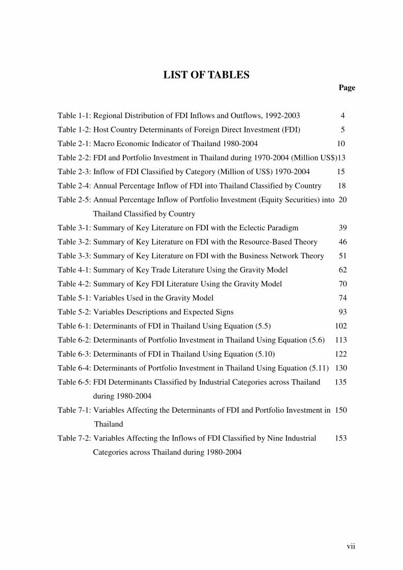
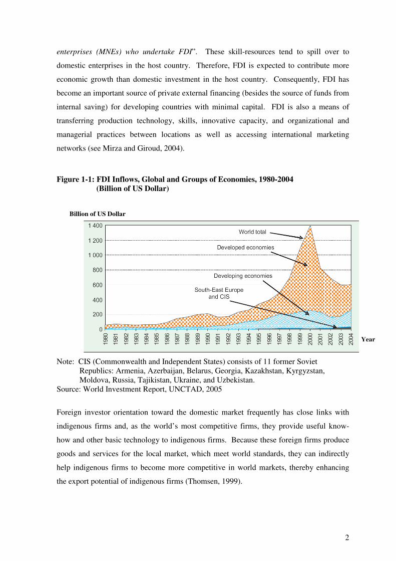
Global Foreign Direct Investment (FDI) flows grew strongly in the 1990s, giving rise to
almost 54,000 transnational corporations, and have since grown rapidly at a rate above
global economic growth rates. Recorded global inflows grew by an average of 13% a year
during 1990-1997, compared with the average rates of 7% both for world exports of goods
and nonfactor services and for world GDP at current prices (Carson, 2003; Mallampally
and Sauvant, 1999). Because of the large numbers of cross-border mergers and
acquisitions (M&A), these inflows increased by an average of nearly 50% a year during
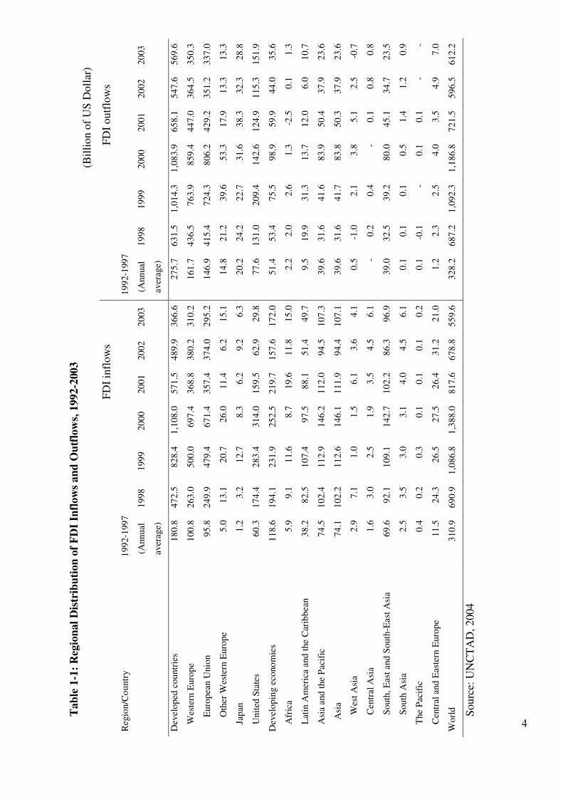
1998-2000, reaching a record of US$ 1.388 trillion in 2000 (see Table 1-1). Inflows
declined to US$ 559.6 billion in 2003, mostly as a result of the sharp drop in cross-border
M&A amongst the developed countries. In addition, the value of cross-border M&A
declined from the record US$ 678.8 billion in 2002 to about US$ 559.6 billion in 2003
(IMF, 2003).
Developed countries have major influences over the FDI inflows and outflows, accounting
for 94% of outflows and over 70% of inflows in 2001 (IMF, 2003). Inflows of FDI to
developing countries grew by an average of 23% a year during 1990-2000 (see Figure 1-1).
In 2001, the inflows declined by 13% to US$ 215 billion (IMF, 2003). The decline,
however, was mostly accounted for by the decline in FDI inflows in three (developing)
economies – Hong Kong, Brazil, and Argentina. This was due to the failure of government
economic policies in Brazil and Argentina, and the outbreak of the illness severe acute
respiratory syndrome (SARS) in Hong Kong (UNCTAD, 2004). Excluding these three
economies, FDI inflows into developing countries increased by about 18% in 2001 (IMF,
2003). During 1998-2001, FDI inflows to developing countries averaged US$ 225 billion
a year (see Table 1-1).
According to Kumar (2003, p. 6) “FDI usually flows as a bundle of resources including,
besides capital, production technology, organizational and managerial skills, marketing
know-how, and even market access through the marketing networks of multinational
2
enterprises (MNEs) who undertake FDI”. These skill-resources tend to spill over to
domestic enterprises in the host country. Therefore, FDI is expected to contribute more
economic growth than domestic investment in the host country. Consequently, FDI has
become an important source of private external financing (besides the source of funds from
internal saving) for developing countries with minimal capital. FDI is also a means of
transferring production technology, skills, innovative capacity, and organizational and
managerial practices between locations as well as accessing international marketing
networks (see Mirza and Giroud, 2004).
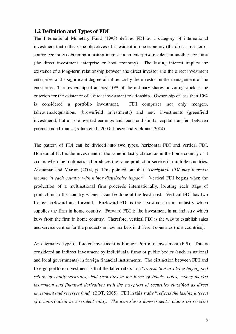
Figure 1-1: FDI Inflows, Global and Groups of Economies, 1980-2004 (Billion of US Dollar)
Note: CIS (Commonwealth and Independent States) consists of 11 former Soviet
Republics: Armenia, Azerbaijan, Belarus, Georgia, Kazakhstan, Kyrgyzstan, Moldova, Russia, Tajikistan, Ukraine, and Uzbekistan.
Source: World Investment Report, UNCTAD, 2005
Foreign investor orientation toward the domestic market frequently has close links with
indigenous firms and, as the world’s most competitive firms, they provide useful know-
how and other basic technology to indigenous firms. Because these foreign firms produce
goods and services for the local market, which meet world standards, they can indirectly
help indigenous firms to become more competitive in world markets, thereby enhancing
the export potential of indigenous firms (Thomsen, 1999).
Year
Billion of US Dollar
3
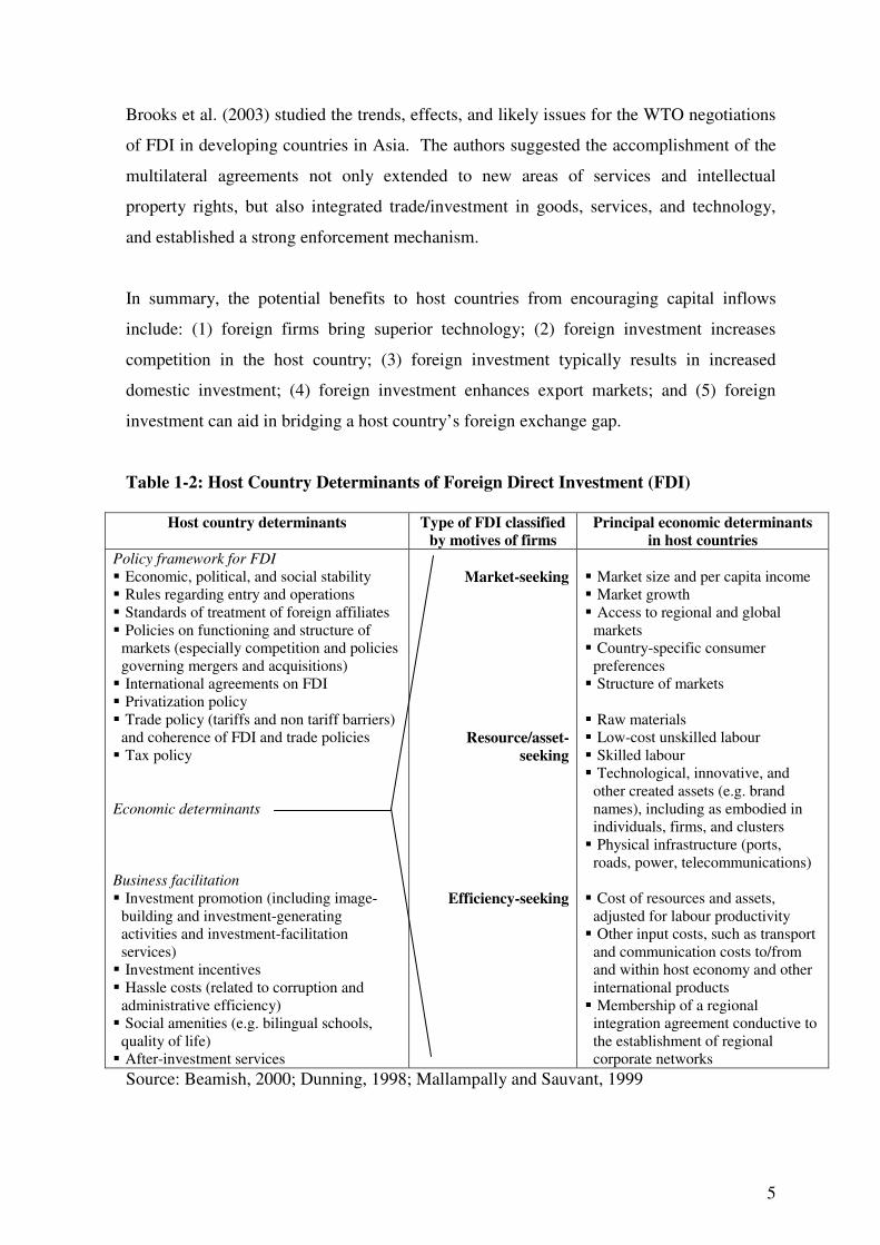
Mallampally and Sauvant (1999) adapted Dunning’s framework (Dunning, 1998, p. 53),
which attempted to summarize the differences between the kind of variables posited to
influence the locational decision of MNEs (see Table 1-2). Table 1-2 presents the reasons
for making a foreign investment in the host countries. Given the potential role of FDI in
accelerated growth, economic transformation, and contribution to economic development,
developing countries are strongly interested in attracting FDI. They are taking steps to
improve the principal determinants and the location choice of foreign direct investment.
Mallampally and Sauvant (1999, p. 36-37) suggested that “countries have begun
liberalizing their national policies to establish a hospitable framework for FDI by relaxing
rules regarding market entry and foreign ownership, improving the standards of treatment
accorded to foreign firms, and improving the functioning of markets. However, equally
important, with FDI policy frameworks becoming more similar, countries interested in
encouraging investment inflows are focusing on measures that facilitate business. These
include investment promotion, investment incentives, after-investment services,
improvements in amenities, and measures that reduce the ‘hassle’ costs of doing
business”.
There are many studies about FDI advantages/disadvantages in the host countries, impact
of FDI on economic growth, and the effects of FDI netflow (see Agarwal and Ramaswami,
1992; Loungani and Razin, 2001; Ismail and Yussof, 2003). Agarwal and Ramaswami
(1992) showed the effects of FDI interrelationship, which implied that firms would like to
establish a market presence in the foreign countries through direct investment. However,
the firms’ abilities were constrained by their size and multinational experience. In
addition, the firms used investment modes only in high potential markets.
Loungani and Razin (2001) suggested that FDI could contribute to investment and growth
in host countries through various channels such as technology transformation, human
capital development by employee training programmes, and corporate tax revenues.
Moreover, developing countries should focus on improving the investment climate in all
kinds of capital, domestic as well as foreign, to attract FDI. Ismail and Yussof (2003)
showed the result with regard to labour market competitiveness; different countries may
require different policy recommendations in order to attract FDI inflows into the countries.
4
Tab
le 1
-1:
Reg
ion
al
Dis
trib
uti
on
of
FD
I In
flow
s an
d O
utf
low
s, 1
992-2
003
(B
illi
on o
f U
S D
oll
ar)
FD
I in
flow
s
F
DI
outf
low
s
Reg
ion/C
oun
try
19
92
-199
7
19
92
-199
7
(A
nn
ual
aver
age)
19
98
1
99
9
20
00
2
00
1
20
02
2
00
3
(Ann
ual
aver
age)
19
98
1
99
9
20
00
2
00
1
20
02
2
00
3
Dev
elo
ped
co
untr
ies
18
0.8
4
72
.5
82
8.4
1
,10
8.0
5
71
.5
48
9.9
3
66
.6
27
5.7
6
31
.5
1,0
14.3
1
,08
3.9
6
58
.1
54
7.6
5
69
.6
W
este
rn E
uro
pe
10
0.8
2
63
.0
50
0.0
6
97
.4
36
8.8
3
80
.2
31
0.2
1
61
.7
43
6.5
7
63
.9
85
9.4
4
47
.0
36
4.5
3
50
.3
E
uro
pea
n U
nio
n
95
.8
24
9.9
4
79
.4
67
1.4
3
57
.4
37
4.0
2
95
.2
14
6.9
4
15
.4
72
4.3
8
06
.2
42
9.2
3
51
.2
33
7.0
O
ther
Wes
tern
Euro
pe
5.0
1
3.1
2
0.7
2
6.0
1
1.4
6
.2
15
.1
14
.8
21
.2
39
.6
53
.3
17
.9
13
.3
13
.3
J
apan
1
.2
3.2
1
2.7
8
.3
6.2
9
.2
6.3
2
0.2
2
4.2
2
2.7
3
1.6
3
8.3
3
2.3
2
8.8
U
nit
ed S
tate
s 6
0.3
1
74
.4
28
3.4
3
14
.0
15
9.5
6
2.9
2
9.8
7
7.6
1
31
.0
20
9.4
1
42
.6
12
4.9
1
15
.3
15
1.9
Dev
elo
pin
g e
cono
mie
s 1
18
.6
19
4.1
2
31
.9
25
2.5
2
19
.7
15
7.6
1
72
.0
51
.4
53
.4
75
.5
98
.9
59
.9
44
.0
35
.6
A
fric
a 5
.9
9.1
1
1.6
8
.7
19
.6
11
.8
15
.0
2.2
2
.0
2.6
1
.3
-2.5
0
.1
1.3
L
atin
Am
eric
a an
d t
he
Car
ibb
ean
38
.2
82
.5
10
7.4
9
7.5
8
8.1
5
1.4
4
9.7
9
.5
19
.9
31
.3
13
.7
12
.0
6.0
1
0.7
A
sia
and
the
Pac
ific
7
4.5
1
02
.4
11
2.9
1
46
.2
11
2.0
9
4.5
1
07
.3
39
.6
31
.6
41
.6
83
.9
50
.4
37
.9
23
.6
Asi
a 7
4.1
1
02
.2
11
2.6
1
46
.1
11
1.9
9
4.4
1
07
.1
39
.6
31
.6
41
.7
83
.8
50
.3
37
.9
23
.6
W
est
Asi
a 2
.9
7.1
1
.0
1.5
6
.1
3.6
4
.1
0.5
-1
.0
2.1
3
.8
5.1
2
.5
-0.7
C
entr
al A
sia
1.6
3
.0
2.5
1
.9
3.5
4
.5
6.1
-
0.2
0
.4
- 0
.1
0.8
0
.8
S
outh
, E
ast
and
So
uth
-Eas
t A
sia
69
.6
92
.1
10
9.1
1
42
.7
10
2.2
8
6.3
9
6.9
3
9.0
3
2.5
3
9.2
8
0.0
4
5.1
3
4.7
2
3.5
S
outh
Asi
a 2
.5
3.5
3
.0
3.1
4
.0
4.5
6
.1
0.1
0
.1
0.1
0
.5
1.4
1
.2
0.9
T
he
Pac
ific
0
.4
0.2
0
.3
0.1
0
.1
0.1
0
.2
0.1
-0
.1
- 0
.1
0.1
-
-
C
entr
al a
nd
Eas
tern
Euro
pe
11
.5
24
.3
26
.5
27
.5
26
.4
31
.2
21
.0
1.2
2
.3
2.5
4
.0
3.5
4
.9
7.0
Wo
rld
3
10
.9
69
0.9
1
,08
6.8
1
,38
8.0
8
17
.6
67
8.8
5
59
.6
32
8.2
6
87
.2
1,0
92.3
1
,18
6.8
7
21
.5
59
6.5
6
12
.2
Sourc
e: U
NC
TA
D, 2004
5
Brooks et al. (2003) studied the trends, effects, and likely issues for the WTO negotiations
of FDI in developing countries in Asia. The authors suggested the accomplishment of the
multilateral agreements not only extended to new areas of services and intellectual
property rights, but also integrated trade/investment in goods, services, and technology,
and established a strong enforcement mechanism.
In summary, the potential benefits to host countries from encouraging capital inflows
include: (1) foreign firms bring superior technology; (2) foreign investment increases
competition in the host country; (3) foreign investment typically results in increased
domestic investment; (4) foreign investment enhances export markets; and (5) foreign
investment can aid in bridging a host country’s foreign exchange gap.
Table 1-2: Host Country Determinants of Foreign Direct Investment (FDI)
Host country determinants Type of FDI classified by motives of firms
Principal economic determinants in host countries
Policy framework for FDI
� Economic, political, and social stability � Rules regarding entry and operations � Standards of treatment of foreign affiliates � Policies on functioning and structure of
markets (especially competition and policies governing mergers and acquisitions)
� International agreements on FDI � Privatization policy � Trade policy (tariffs and non tariff barriers)
and coherence of FDI and trade policies � Tax policy Economic determinants
Market-seeking
Resource/asset-seeking
� Market size and per capita income � Market growth � Access to regional and global
markets � Country-specific consumer
preferences � Structure of markets � Raw materials � Low-cost unskilled labour � Skilled labour � Technological, innovative, and
other created assets (e.g. brand names), including as embodied in individuals, firms, and clusters
� Physical infrastructure (ports, roads, power, telecommunications)
Business facilitation
� Investment promotion (including image-building and investment-generating activities and investment-facilitation services)
� Investment incentives � Hassle costs (related to corruption and
administrative efficiency) � Social amenities (e.g. bilingual schools,
quality of life) � After-investment services
Efficiency-seeking
� Cost of resources and assets,
adjusted for labour productivity � Other input costs, such as transport
and communication costs to/from and within host economy and other international products
� Membership of a regional integration agreement conductive to the establishment of regional corporate networks
Source: Beamish, 2000; Dunning, 1998; Mallampally and Sauvant, 1999
6
1.2 Definition and Types of FDI
The International Monetary Fund (1993) defines FDI as a category of international
investment that reflects the objectives of a resident in one economy (the direct investor or
source economy) obtaining a lasting interest in an enterprise resident in another economy
(the direct investment enterprise or host economy). The lasting interest implies the
existence of a long-term relationship between the direct investor and the direct investment
enterprise, and a significant degree of influence by the investor on the management of the
enterprise. The ownership of at least 10% of the ordinary shares or voting stock is the
criterion for the existence of a direct investment relationship. Ownership of less than 10%
is considered a portfolio investment. FDI comprises not only mergers,
takeovers/acquisitions (brownfield investments) and new investments (greenfield
investment), but also reinvested earnings and loans and similar capital transfers between
parents and affiliates (Adam et al., 2003; Jansen and Stokman, 2004).
The pattern of FDI can be divided into two types, horizontal FDI and vertical FDI.
Horizontal FDI is the investment in the same industry abroad as in the home country or it
occurs when the multinational produces the same product or service in multiple countries.
Aizenman and Marion (2004, p. 126) pointed out that “Horizontal FDI may increase
income in each country with minor distributive impact”. Vertical FDI begins when the
production of a multinational firm proceeds internationally, locating each stage of
production in the country where it can be done at the least cost. Vertical FDI has two
forms: backward and forward. Backward FDI is the investment in an industry which
supplies the firm in home country. Forward FDI is the investment in an industry which
buys from the firm in home country. Therefore, vertical FDI is the way to establish sales
and service centres for the products in new markets in different countries (host countries).
An alternative type of foreign investment is Foreign Portfolio Investment (FPI). This is
considered an indirect investment by individuals, firms or public bodies (such as national
and local governments) in foreign financial instruments. The distinction between FDI and
foreign portfolio investment is that the latter refers to a “transaction involving buying and
selling of equity securities, debt securities in the forms of bonds, notes, money market
instrument and financial derivatives with the exception of securities classified as direct
investment and reserves fund” (BOT, 2005). FDI in this study “reflects the lasting interest
of a non-resident in a resident entity. The item shows non-residents’ claims on resident
7
entities and thus is recorded as the country’s external liabilities” (BOT, 2005). In
addition, Dunning (1988) criticized FDI, saying that it concerned issues of direct control
since resources were transferred internally within firms rather than externally between
independent firms. Haddad and Harrison (1993) proved that the benefits from FDI are not
equally distributed in developing countries. Policies should be developed to avoid
inequality, encourage efficiency of domestic firms, benefit from linkages with and
spillovers from foreign firms, and attract FDI into areas or categories that are most likely to
benefit the poor such as in rural areas or agricultural processing.
1.3 Interest of the Research
There has been limited research on the determinants of FDI in Thailand. Previous research
addressed factors that are important to FDI in the Thai economy (see Brimble and
Sibunruang, 2002; Lauridsen, 2004) and the effects of foreign investment in Thailand (see
Jansen ,2003). However, these studies focused only on the foreign investment at either the
sectoral level or national level. No research has focused on both levels. For example,
according to the Jansen (2003) study, the inflows of capital investment into Thailand are
associated with higher asset prices, lower lending rates, and domestic spending driven by
higher foreign investment. In addition, the Lauridsen (2004) study shows that FDI plays a
significant role in Thailand FDI development, which contributed to the long-term
competitiveness and sustainability growth of the country during the 1990s. Lauridsen
(2004) study is concerned with the extent to which the Thai government was able to
formulate and in particular implement a credible and adequate set of linkage and supplier
development policies. This study examines the role of FDI in Thailand and the factors that
determine FDI across industrial categories in Thailand.
1.4 Purpose of the Research
The general objective of this research is to evaluate the determinants of FDI and portfolio
investment in Thailand. It also examines the FDI flows between different locations and
their geographical distance in Thailand. The primary research question addresses what
factors motivate, attract, and sustain foreign investments in Thailand.
8
The specific objectives of this research include:
1. To provide an overview of foreign direct investment (FDI) studies, such as the
Eclectic Paradigm, Resourced-based Theory, and Business Network Theory, which
help to explain the patterns of FDI in Thailand and the Gravity Model;
2. To evaluate the determinants of FDI inflows and foreign portfolio investment (FPI)
into Thailand using an extended Gravity Model;
3. To examine the effects of the 1997 Asian financial crisis on the FDI and foreign
portfolio investment (FPI) in Thailand;
4. To provide policy recommendations to policy makers for improving Thailand’s
investment climate to attract inflow of FDI.
1.5 Organisation of the Research
This thesis is organised into seven chapters. Chapter 1 presents the introduction, the
objectives of the research, and the scope of the work. Chapter 2 describes the industrial
patterns of FDI and portfolio investment in Thailand from 1980 to 2004. Chapter 3
reviews the conventional FDI literature based on the Eclectic Paradigm, Resource-Based
Theory, and Business Network Theory. Chapter 4 provides an overview of the Gravity
Model in trade and FDI, which will be used to develop the empirical models in the next
chapter. Chapter 5 describes the data collection and research methodology. Chapter 6
presents the results of the research and discusses the research findings. Chapter 7
summarises the research findings and presents the conclusions. The chapter also discusses
the contributions of the research, the theoretical implications, limitations of the research,
and suggestions for future research.
CHAPTER 2
HISTORICAL DESCRIPTION OF FDI IN THAILAND This chapter provides an economic overview of Thailand; the overall patterns of FDI
inflow and the inflow of portfolio investment; the stages of FDI policy and the impact of
investment policy on FDI. The data for FDI and portfolio investment in Thailand are
provided and further FDI data by categories (industry, financial institutions, trade, mining
and quarrying, agricultural products, services, investment, real estate, and others) are also
provided with a brief explanation.
2.1 An Economic Overview of Thailand
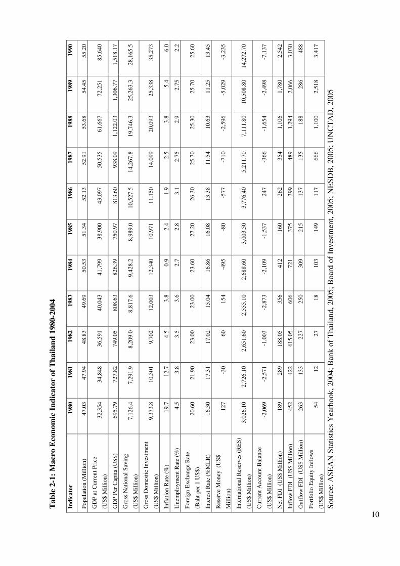
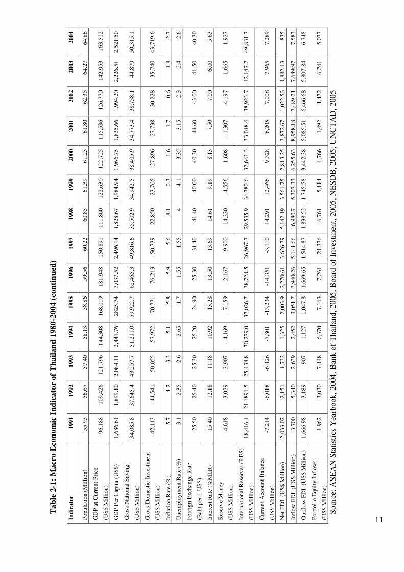
Thailand’s real GDP rose by 6.3% in 2004 and increased to 7% in 2005 (BOT, 2005).
Growth in 2006 was 7.3% and inflation was 1.3% in 2005, a decrease from 2.7% in 2004
(see Table 2-1). Since 2003, economic performance in Thailand has recovered fully from
the 1997 Asian Financial Crisis. With its first fiscal surplus in 2003, the factors that
contributed to the surplus included strong economic growth, improvements in tax
administration and collection, falling debt service costs and the expiration of a five-year
period when companies were allowed to carry over losses incurred during their insolvency.
Exports accelerated in 2004 because global economic conditions keep improving and
appreciation of the Thai Baht was kept in check. The increase in government investment
in 2005 further contributed to economic growth and development. However, the rises of
interest rates to cap inflationary pressures and other measures to curb the rise of household
debt dampened the growth toward the end of 2004 and into 2005, including the inflow of
FDI.
Over the past few decades, the FDI inflow into Thailand has accelerated rapidly. There
was a large increase in FDI at the end of the 1980s until the late 1990s (before the Asian
Financial Crisis in 1997), from US$ 489 million in 1987 through US$ 1,294 million in
1988 to a peak in 1998 (US$ 7 billion) (see Table 2-1). This figure decreased slightly over
the following two years, but the value of FDI in 2001 was higher than it was in 1998.
Recently, the amount of FDI has been small but the GNP, exports of goods and services
(XGS), and reserve money became significantly larger (see Table 2-1). Thus, this may
imply that FDI will play an increasingly important role in Thailand’s economy in the future
(Hongskul, 2000).
10
Tab
le 2
-1:
Macr
o E
con
om
ic I
nd
icato
r of
Th
ail
an
d 1
980-2
004
Ind
icato
r 1
980
1
981
1
982
1
983
1
984
1
985
1
986
1
987
1
988
1
989
1
990
Po
pu
lati
on
(M
illi
on
) 4
7.0
3
47
.94
4
8.8
3
49
.69
5
0.5
3
51
.34
5
2.1
3
52
.91
5
3.6
8
54
.45
5
5.2
0
GD
P a
t C
urr
ent
Pri
ce
(US
$ M
illi
on
) 3
2,3
54
3
4,8
48
3
6,5
91
4
0,0
43
4
1,7
99
3
8,9
00
4
3,0
97
5
0,5
35
6
1,6
67
7
2,2
51
8
5,6
40
GD
P P
er C
apit
a (U
S$
) 6
95.7
9
72
7.8
2
74
9.0
5
80
8.6
3
82
6.3
9
75
0.9
7
81
3.6
0
93
8.0
9
1,1
22
.03
1
,30
6.7
7
1,5
18
.17
Gro
ss N
atio
nal
Sav
ing
(US
$ M
illi
on
) 7
,12
6.4
7
,29
1.9
8
,20
9.0
8
,81
7.6
9
,42
8.2
8
,98
9.0
1
0,5
27
.5
14
,267
.8
19
,746
.3
25
,263
.3
28
,165
.5
Gro
ss D
om
esti
c In
ves
tmen
t
(US
$ M
illi
on
) 9
,37
3.8
1
0,3
01
9
,70
2
12
,003
1
2,3
40
1
0,9
71
1
1,1
50
1
4,0
99
2
0,0
93
2
5,3
38
3
5,2
73
Infl
atio
n R
ate
(%)
19
.7
12
.7
4.5
3
.8
0.9
2
.4
1.9
2
.5
3.8
5
.4
6.0
Un
emp
loym
ent
Rat
e (%
) 4
.5
3.8
3
.5
3.6
2
.7
2.8
3
.1
2.7
5
2.9
2
.75
2
.2
Fo
reig
n E
xch
ange
Rat
e
(Bah
t p
er 1
US
$)
20
.60
2
1.9
0
23
.00
2
3.0
0
23
.60
2
7.2
0
26
.30
2
5.7
0
25
.30
2
5.7
0
25
.60
Inte
rest
Rat
e (%
ML
R)
16
.30
1
7.3
1
17
.02
1
5.0
4
16
.86
1
6.0
8
13
.38
1
1.5
4
10
.63
1
1.2
5
13
.45
Res
erv
e M
on
ey
(US
$
Mil
lion
) 1
27
-3
0
60
1
54
-4
95
-8
0
-577
-7
10
-2
,59
6
-5,0
29
-3
,23
5
Inte
rnat
ion
al R
eser
ves
(R
ES
)
(US
$ M
illi
on
) 3
,02
6.1
0
2,7
26
.10
2
,65
1.6
0
2,5
55
.10
2
,68
8.6
0
3,0
03
.50
3
,77
6.4
0
5,2
11
.70
7
,11
1.8
0
10
,508
.80
1
4,2
72
.70
Cu
rren
t A
cco
un
t B
alan
ce
(US
$ M
illi
on
) -2
,06
9
-2,5
71
-1
,00
3
-2,8
73
-2
,10
9
-1,5
37
2
47
-3
66
-1
,65
4
-2,4
98
-7
,13
7
Net
FD
I (
US
$ M
illi
on
) 1
89
2
89
1
88.0
5
35
6
41
2
16
0
26
2
35
4
1,1
06
1
,78
0
2,5
42
Infl
ow
FD
I (
US
$ M
illi
on
) 4
52
4
22
4
15.0
5
60
6
72
1
37
5
39
9
48
9
1,2
94
2
,06
6
3,0
30
Ou
tflo
w F
DI
(U
S$
Mil
lion
) 2
63
1
33
2
27
2
50
3
09
2
15
1
37
1
35
1
88
2
86
4
88
Po
rtfo
lio E
qu
ity I
nfl
ow
s
(US
$ M
illi
on
) 5
4
12
2
7
18
1
03
1
49
1
17
6
66
1
,10
0
2,5
18
3
,41
7
Sourc
e: A
SE
AN
Sta
tist
ics
Yea
rbook, 2004;
Ban
k o
f T
hai
land, 2005;
Bo
ard
of
Inves
tmen
t, 2
005;
NE
SD
B, 2005;
UN
CT
AD
, 2
005
11
Tab
le 2
-1:
Macr
o E
con
om
ic I
nd
icato
r of
Th
ail
an
d 1
980-2
004 (
con
tin
ued
)
Ind
icato
r 1
991
1
992
1
993
1
994
1
995
1
996
1
997
1
998
1
999
2
000
2
001
2
002
2
003
2
004
Po
pu
lati
on
(M
illi
on
) 5
5.9
3
56
.67
5
7.4
0
58
.13
5
8.8
6
59
.56
6
0.2
2
60
.85
6
1.3
9
61
.23
6
1.8
0
62
.35
6
4.2
7
64
.86
GD
P a
t C
urr
ent
Pri
ce
(US
$ M
illi
on
) 9
6,1
88
1
09,4
26
1
21,7
96
1
44,3
08
1
68,0
19
1
81,9
48
1
50,8
91
1
11,8
60
1
22,6
30
1
22,7
25
1
15,5
36
1
26,7
70
1
42,9
53
1
63,5
12
GD
P P
er C
apit
a (U
S$
) 1
,68
6.6
1
1,8
99
.10
2
,08
4.1
1
2,4
41
.76
2
825
.74
3
,03
7.5
2
2,4
96
.14
1
,82
8.6
7
1,9
84
.94
1
,96
6.7
5
1,8
35
.66
1
,99
4.2
0
2,2
26
.51
2
,52
1.5
0
Gro
ss N
atio
nal
Sav
ing
(US
$ M
illi
on
) 3
4,0
85
.8
37
,645
.4
43
,257
.7
51
,211
.0
59
,922
.7
62
,465
.3
49
,816
.6
35
,502
.9
34
,942
.5
38
,405
.9
34
,773
.4
38
,758
.1
44
,879
5
0,3
15
.1
Gro
ss D
om
esti
c In
ves
tmen
t
(US
$ M
illi
on
) 4
2,1
13
4
4,5
41
5
0,0
55
5
7,9
72
7
0,7
71
7
6,2
13
5
0,7
39
2
2,8
50
2
3,7
65
2
7,8
96
2
7,7
38
3
0,2
28
3
5,7
40
4
3,7
19
.6
Infl
atio
n R
ate
(%)
5.7
4
.2
3.3
5
.1
5.8
5
.9
5.6
8
.1
0.3
1
.6
1.7
0
.6
1.8
2
.7
Un
emp
loym
ent
Rat
e (%
) 3
.1
2.3
5
2.6
2
.65
1
.7
1.5
5
1.5
5
4
4.1
3
.35
3
.15
2
.3
2.4
2
.6
Fo
reig
n E
xch
ange
Rat
e
(Bah
t p
er 1
US
$)
25
.50
2
5.4
0
25
.30
2
5.2
0
24
.90
2
5.3
0
31
.40
4
1.4
0
40
.00
4
0.3
0
44
.60
4
3.0
0
41
.50
4
0.3
0
Inte
rest
Rat
e (%
ML
R)
15
.40
1
2.1
8
11
.18
1
0.9
2
13
.28
1
3.5
0
13
.69
1
4.6
1
9.1
9
8.1
3
7.5
0
7.0
0
6.0
0
5.6
3
Res
erv
e M
on
ey
(US
$ M
illi
on
) -4
,61
8
-3,0
29
-3
,90
7
-4,1
69
-7
,15
9
-2,1
67
9
,90
0
-14
,330
-4
,55
6
1,6
08
-1
,30
7
-4,1
97
-1
,66
5
1,9
27
Inte
rnat
ion
al R
eser
ves
(R
ES
)
(US
$ M
illi
on
) 1
8,4
16
.4
21
,189
1.5
2
5,4
38
.8
30
,279
.0
37
,026
.7
38
,724
.5
26
,967
.7
29
,535
.9
34
,780
.6
32
,661
.3
33
,048
.4
38
,923
.7
42
,147
.7
49
,831
.7
Cu
rren
t A
cco
un
t B
alan
ce
(US
$ M
illi
on
) -7
,21
4
-6,0
18
-6
,12
6
-7,8
01
-1
3,2
34
-1
4,3
51
-3
,11
0
14
,291
1
2,4
66
9
,32
8
6,2
05
7
,00
8
7,9
65
7
,28
9
Net
FD
I (
US
$ M
illi
on
) 2
,03
3.0
2
2,1
51
1
,73
2
1,3
25
2
,00
3.9
2
,27
0.6
1
3,6
26
.79
5
,14
2.1
9
3,5
61
.75
2
,81
3.2
5
3,8
72
.67
1
,02
2.5
3
1,8
82
.13
8
35
Infl
ow
FD
I (
US
$ M
illi
on
) 3
,70
0
5,3
40
2
,63
9
2,4
52
3
,05
1.7
3
,94
0.2
6
5,1
41
.66
6
,98
0.7
5
,30
7.3
3
6,2
55
.63
8
,95
8.1
8
7,4
89
.21
7
,68
9.9
7
7,5
83
Ou
tflo
w F
DI
(U
S$
Mil
lion
) 1
,66
6.9
8
3,1
89
9
07
1
,12
7
1,0
47
.8
1,6
69
.65
1
,51
4.8
7
1,8
38
.52
1
,74
5.5
8
3,4
42
.38
5
,08
5.5
1
6,4
66
.68
5
,80
7.8
4
6,7
48
Po
rtfo
lio E
qu
ity I
nfl
ow
s
(US
$ M
illi
on
) 1
,96
2
3,0
30
7
,14
8
6,3
70
7
,16
3
7,2
61
2
1,3
76
6
,76
1
5,1
14
4
,76
6
1,4
92
1
,47
2
6,2
41
5
,07
7
Sourc
e: A
SE
AN
Sta
tist
ics
Yea
rbook, 2004;
Ban
k o
f T
hai
land, 2005;
Bo
ard
of
Inves
tmen
t, 2
005;
NE
SD
B, 2005;
UN
CT
AD
, 2
005
12
2.2 Foreign Investment in Thailand
Historically, Thailand has depended heavily on the inflows of FDI from the United States
and Japan, which accounted for at least 50% of all FDI inflow. This geographic pattern of
FDI has changed remarkably since the early 1980s when Japan was looking for production
bases abroad to escape appreciating home currencies. Thailand’s FDI in recent years is
geographically diversified with new partners including ASEAN, EU-151, Australia, and
New Zealand.
Thailand has been open to the international economy since the 1990s, as indicated by both
the increase in FDI and rising GDP. Thailand is among a small group of developing
economies classified by Sachs et al. (1995, p. 22) as “always open”. That is, it exhibits
very high trade orientation, welcomes foreign investors, and has low average tariffs,
modest interindustry tariff distribution and investment incidence of nontrade barriers.
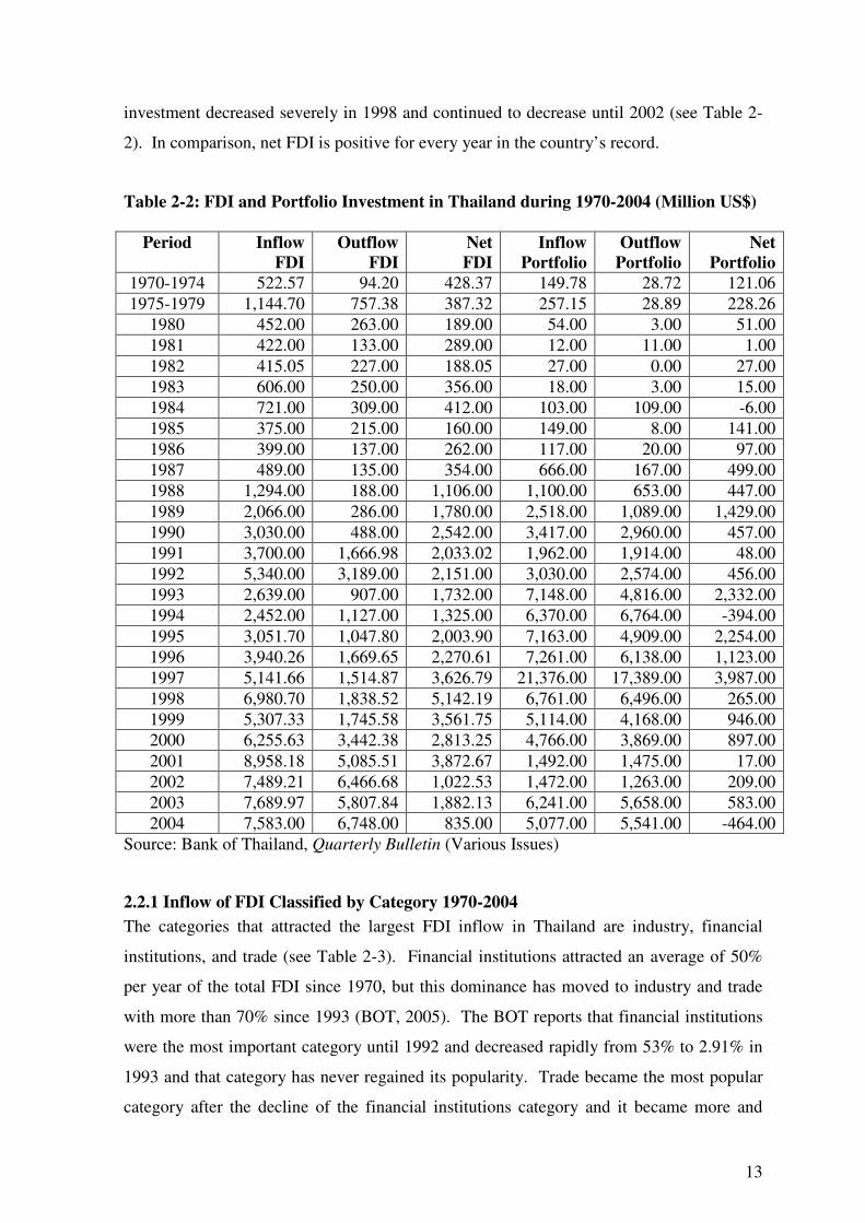
Table 2-2 shows the historic distribution of FDI flows to Thailand since 1970. The annual
FDI flows to Thailand started to exceed US$ 523 million in the early 1970s, and increased
to US$ 1,300 million in 1988. Inflow of FDI to Thailand increased from around US$ 500
million during 1970-1974 to almost US$ 20 billion during 1995-1998, but decreased
slightly to US$ 5,300 million in 1999 (see Table 2-2). The outflow of FDI increased
dramatically in 1991 with a reduction in 1993. Furthermore, Table 2-2 shows portfolio
investment in Thailand is insignificant compared to FDI during 1980-1986. However, the
portfolio investment inflow increased significantly in 1987, and in 1997, increased in both
inflow and outflow. Since then, the net portfolio investment has decreased from US$ 4,000
million in 1997 to US$ 265 million in 1998. This is because of the effects of the 1997
Asian Financial which caused the inflows of portfolio investment into Thailand to decrease
dramatically from US$ 21.3 million in 1997 to US$ 6.8 million in 1998. The consistent
positive net portfolio investment indicates that foreign firms have great confidence in
investing into the Thai economy, the only exceptions being in 1984 and 1994. In 1997, the
inflow and outflow of portfolio investment increased threefold from the previous year.
However, because of the Asian Financial Crisis effect in mid 1997, the portfolio
1 Austria, Belgium, Denmark, Finland, France, Germany, Greece, Ireland (Republic of), Italy, Luxembourg, Netherlands, Portugal, Spain, Sweden and United Kingdom
13
investment decreased severely in 1998 and continued to decrease until 2002 (see Table 2-
2). In comparison, net FDI is positive for every year in the country’s record.
Table 2-2: FDI and Portfolio Investment in Thailand during 1970-2004 (Million US$)
Period Inflow FDI
Outflow FDI
Net FDI
Inflow Portfolio
Outflow Portfolio
Net Portfolio
1970-1974 522.57 94.20 428.37 149.78 28.72 121.06
1975-1979 1,144.70 757.38 387.32 257.15 28.89 228.26
1980 452.00 263.00 189.00 54.00 3.00 51.00
1981 422.00 133.00 289.00 12.00 11.00 1.00
1982 415.05 227.00 188.05 27.00 0.00 27.00
1983 606.00 250.00 356.00 18.00 3.00 15.00
1984 721.00 309.00 412.00 103.00 109.00 -6.00
1985 375.00 215.00 160.00 149.00 8.00 141.00
1986 399.00 137.00 262.00 117.00 20.00 97.00
1987 489.00 135.00 354.00 666.00 167.00 499.00
1988 1,294.00 188.00 1,106.00 1,100.00 653.00 447.00
1989 2,066.00 286.00 1,780.00 2,518.00 1,089.00 1,429.00
1990 3,030.00 488.00 2,542.00 3,417.00 2,960.00 457.00
1991 3,700.00 1,666.98 2,033.02 1,962.00 1,914.00 48.00
1992 5,340.00 3,189.00 2,151.00 3,030.00 2,574.00 456.00
1993 2,639.00 907.00 1,732.00 7,148.00 4,816.00 2,332.00
1994 2,452.00 1,127.00 1,325.00 6,370.00 6,764.00 -394.00
1995 3,051.70 1,047.80 2,003.90 7,163.00 4,909.00 2,254.00
1996 3,940.26 1,669.65 2,270.61 7,261.00 6,138.00 1,123.00
1997 5,141.66 1,514.87 3,626.79 21,376.00 17,389.00 3,987.00
1998 6,980.70 1,838.52 5,142.19 6,761.00 6,496.00 265.00
1999 5,307.33 1,745.58 3,561.75 5,114.00 4,168.00 946.00
2000 6,255.63 3,442.38 2,813.25 4,766.00 3,869.00 897.00
2001 8,958.18 5,085.51 3,872.67 1,492.00 1,475.00 17.00
2002 7,489.21 6,466.68 1,022.53 1,472.00 1,263.00 209.00
2003 7,689.97 5,807.84 1,882.13 6,241.00 5,658.00 583.00
2004 7,583.00 6,748.00 835.00 5,077.00 5,541.00 -464.00
Source: Bank of Thailand, Quarterly Bulletin (Various Issues)
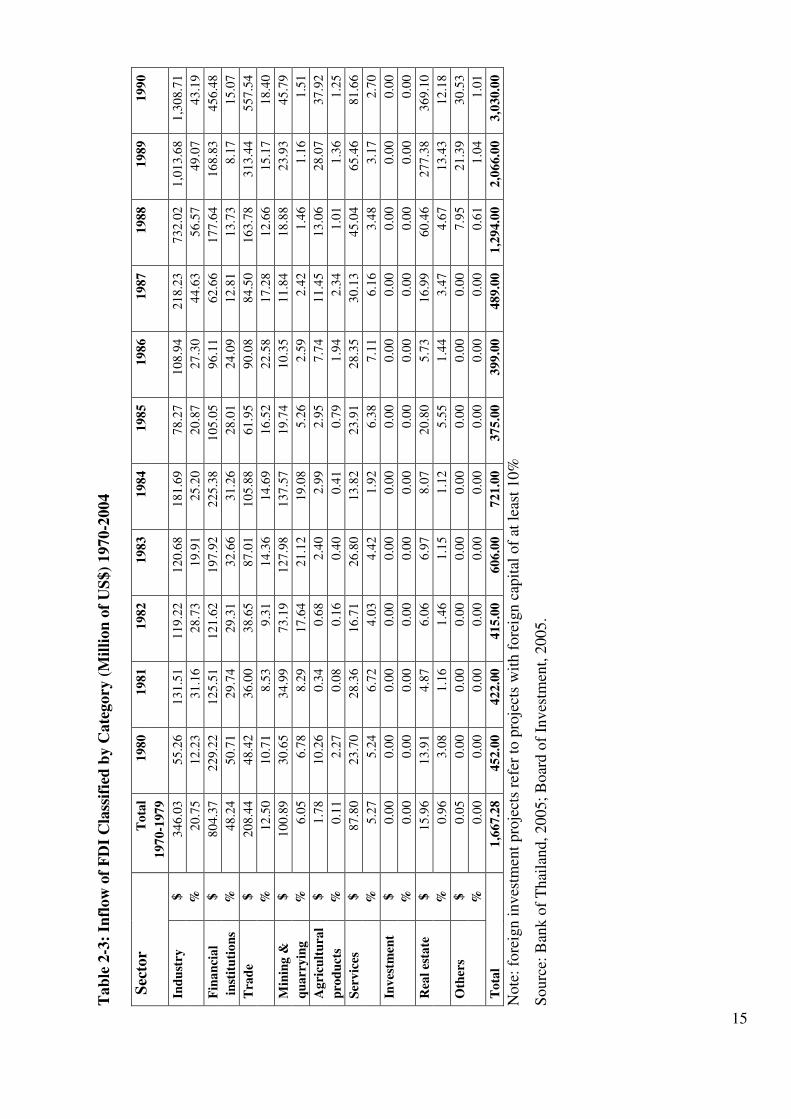
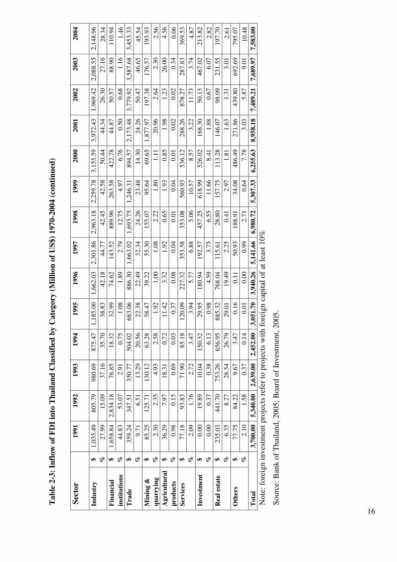
2.2.1 Inflow of FDI Classified by Category 1970-2004
The categories that attracted the largest FDI inflow in Thailand are industry, financial
institutions, and trade (see Table 2-3). Financial institutions attracted an average of 50%
per year of the total FDI since 1970, but this dominance has moved to industry and trade
with more than 70% since 1993 (BOT, 2005). The BOT reports that financial institutions
were the most important category until 1992 and decreased rapidly from 53% to 2.91% in
1993 and that category has never regained its popularity. Trade became the most popular
category after the decline of the financial institutions category and it became more and
14
0
1,000
2,000
3,000
4,000
5,000
6,000
7,000
8,000
9,000
10,000
Year
millions o
f U
S$
Inflow FDI
Outflow FDI
Net FDI
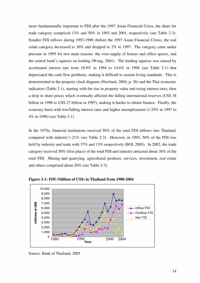
more fundamentally important to FDI after the 1997 Asian Financial Crisis, the share for
trade category comprised 13% and 50% in 1993 and 2001, respectively (see Table 2-3).
Smaller FDI inflows during 1993-1996 (before the 1997 Asian Financial Crisis), the real
estate category decreased to 30% and dropped to 2% in 1997. The category came under
pressure in 1995 for two main reasons: the over-supply of houses and office spaces, and
the central bank’s squeeze on lending (Wong, 2001). The lending squeeze was caused by
accelerated interest rate from 10.9% in 1994 to 14.6% in 1998 (see Table 2-1) that
depreciated the cash flow problems, making it difficult to sustain living standards. This is
demonstrated in the property clock diagram (Newland, 2004, p. 26) and the Thai economic
indicators (Table 2-1), starting with the rise in property value and rising interest rates, then
a drop in share prices which eventually affected the falling international reserves (US$ 38
billion in 1996 to US$ 27 billion in 1997), making it harder to obtain finance. Finally, the
economy burst with low/falling interest rates and higher unemployment (1.55% in 1997 to
4% in 1998) (see Table 2-1).
In the 1970s, financial institutions received 50% of the total FDI inflows into Thailand,
compared with industry’s 21% (see Table 2-3). However, in 1993, 50% of the FDI was
held by industry and trade with 37% and 13% respectively (BOI, 2005). In 2002, the trade
category received 50% (first place) of the total FDI and industry attracted about 30% of the
total FDI. Mining and quarrying, agricultural products, services, investment, real estate
and others comprised about 20% (see Table 2-3).
Figure 2-1: FDI (Million of US$) in Thailand from 1980-2004 Source: Bank of Thailand, 2005
1980 1990 2000 2004
15
Tab
le 2
-3:
Infl
ow
of
FD
I C
lass
ifie
d b
y C
ate
gory
(M
illi
on
of
US
$)
1970-2
004
Sec
tor
To
tal
1
98
0
19
81
1
98
2
19
83
1
98
4
19
85
1
98
6
19
87
1
98
8
19
89
1
99
0
19
70-1
97
9
Ind
ust
ry
$
34
6.0
3
55
.26
1
31
.51
1
19
.22
1
20
.68
1
81
.69
7
8.2
7
10
8.9
4
21
8.2
3
73
2.0
2
1,0
13.6
8
1,3
08.7
1
%
2
0.7
5
12
.23
3
1.1
6
28
.73
1
9.9
1
25
.20
2
0.8
7
27
.30
4
4.6
3
56
.57
4
9.0
7
43
.19
Fin
an
cia
l $
8
04
.37
2
29
.22
1
25
.51
1
21
.62
1
97
.92
2
25
.38
1
05
.05
9
6.1
1
62
.66
1
77
.64
1
68
.83
4
56
.48
in
stit
uti
on
s %
4
8.2
4
50
.71
2
9.7
4
29
.31
3
2.6
6
31
.26
2
8.0
1
24
.09
1
2.8
1
13
.73
8
.17
1
5.0
7
Tra
de
$
20
8.4
4
48
.42
3
6.0
0
38
.65
8
7.0
1
10
5.8
8
61
.95
9
0.0
8
84
.50
1
63
.78
3
13
.44
5
57
.54
%
1
2.5
0
10
.71
8
.53
9
.31
1
4.3
6
14
.69
1
6.5
2
22
.58
1
7.2
8
12
.66
1
5.1
7
18
.40
Min
ing
&
$
10
0.8
9
30
.65
3
4.9
9
73
.19
1
27
.98
1
37
.57
1
9.7
4
10
.35
1
1.8
4
18
.88
2
3.9
3
45
.79
qu
arr
yin
g
%
6.0
5
6.7
8
8.2
9
17
.64
2
1.1
2
19
.08
5
.26
2
.59
2
.42
1
.46
1
.16
1
.51
Ag
ricu
ltu
ral
$
1.7
8
10
.26
0
.34
0
.68
2
.40
2
.99
2
.95
7
.74
1
1.4
5
13
.06
2
8.0
7
37
.92
pro
du
cts
%
0.1
1
2.2
7
0.0
8
0.1
6
0.4
0
0.4
1
0.7
9
1.9
4
2.3
4
1.0
1
1.3
6
1.2
5
Ser
vic
es
$
87
.80
2
3.7
0
28
.36
1
6.7
1
26
.80
1
3.8
2
23
.91
2
8.3
5
30
.13
4
5.0
4
65
.46
8
1.6
6
%
5
.27
5
.24
6
.72
4
.03
4
.42
1
.92
6
.38
7
.11
6
.16
3
.48
3
.17
2
.70
Inv
estm
ent
$
0.0
0
0.0
0
0.0
0
0.0
0
0.0
0
0.0
0
0.0
0
0.0
0
0.0
0
0.0
0
0.0
0
0.0
0
%
0
.00
0
.00
0
.00
0
.00
0
.00
0
.00
0
.00
0
.00
0
.00
0
.00
0
.00
0
.00
Rea
l es
tate
$
1
5.9
6
13
.91
4
.87
6
.06
6
.97
8
.07
2
0.8
0
5.7
3
16
.99
6
0.4
6
27
7.3
8
36
9.1
0
%
0
.96
3
.08
1
.16
1
.46
1
.15
1
.12
5
.55
1
.44
3
.47
4
.67
1
3.4
3
12
.18
Oth
ers
$
0.0
5
0.0
0
0.0
0
0.0
0
0.0
0
0.0
0
0.0
0
0.0
0
0.0
0
7.9
5
21
.39
3
0.5
3
%
0
.00
0
.00
0
.00
0
.00
0
.00
0
.00
0
.00
0
.00
0
.00
0
.61
1
.04
1
.01
To
tal
1
,66
7.2
8
45
2.0
0
42
2.0
0
41
5.0
0
60
6.0
0
72
1.0
0
37
5.0
0
39
9.0
0
48
9.0
0
1,2
94.0
0
2,0
66.0
0
3,0
30.0
0
Note
: fo
reig
n i
nves
tmen
t pro
ject
s re
fer
to p
roje
cts
wit
h f
ore
ign c
apit
al o
f at
lea
st 1
0%
Sourc
e: B
ank o
f T
hai
lan
d, 2005;
Boar
d o
f In
ves
tmen
t, 2
005.
16
Tab
le 2
-3:
Infl
ow
of
FD
I in
to T
hail
an
d C
lass
ifie
d b
y C
ate
gory
(M
illi
on
of
US
$)
1970-2
004 (
con
tin
ued
) S
ecto
r
1
99
1
19
92
1
99
3
19
94
1
99
5
19
96
1
99
7
19
98
1
99
9
20
00
2
00
1
20
02
2
00
3
20
04
Ind
ust
ry
$
1,0
35.4
9
80
5.7
9
98
0.6
9
87
5.4
7
1,1
85.0
0
1,6
62.0
3
2,3
01.8
6
2,9
63.1
8
2,2
59.7
8
3,1
55.5
9
3,9
72.4
3
1,9
69.4
2
2,0
88.5
5
2,1
48.9
6
%
2
7.9
9
15
.09
3
7.1
6
35
.70
3
8.8
3
42
.18
4
4.7
7
42
.45
4
2.5
8
50
.44
4
4.3
4
26
.30
2
7.1
6
28
.34
Fin
an
cia
l $
1
,65
8.8
4
2,8
34.1
8
76
.85
1
8.3
2
32
.99
7
4.6
2
14
3.5
2
88
9.9
6
26
3.5
8
42
2.7
8
44
.87
5
0.5
7
88
.90
1
10
.94
inst
itu
tio
ns
%
44
.83
5
3.0
7
2.9
1
0.7
5
1.0
8
1.8
9
2.7
9
12
.75
4
.97
6
.76
0
.50
0
.68
1
.16
1
.46
Tra
de
$
35
9.2
4
34
7.5
1
35
0.7
7
50
4.0
2
68
3.0
6
88
6.3
0
1,6
63.0
2
1,6
93.7
5
1,2
46.3
1
89
4.5
7
2,1
73.4
8
3,7
79.9
2
3,5
87.6
8
3,4
53.3
3
%
9
.71
6
.51
1
3.2
9
20
.56
2
2.3
8
22
.49
3
2.3
4
24
.26
2
3.4
8
14
.30
2
4.2
6
50
.47
4
6.6
5
45
.54
Min
ing
&
$
85
.25
1
25
.71
1
30
.12
6
3.2
8
58
.47
3
9.2
2
55
.30
1
55
.07
9
5.6
4
69
.65
1
,87
7.9
7
19
7.3
8
17
6.5
7
19
3.9
3
qu
arr
yin
g
%
2.3
0
2.3
5
4.9
3
2.5
8
1.9
2
1.0
0
1.0
8
2.2
2
1.8
0
1.1
1
20
.96
2
.64
2
.30
2
.56
Ag
ricu
ltu
ral
$
36
.29
7
.97
1
8.3
1
0.7
2
11
.42
3
.32
1
.92
0
.65
1
.93
0
.85
1
.98
1
.23
2
6.0
0
4.5
6
pro
du
cts
%
0.9
8
0.1
5
0.6
9
0.0
3
0.3
7
0.0
8
0.0
4
0.0
1
0.0
4
0.0
1
0.0
2
0.0
2
0.3
4
0.0
6
Ser
vic
es
$
77
.18
9
3.8
3
71
.90
8
5.1
8
12
0.0
9
22
7.3
2
35
3.5
8
35
3.0
8
56
0.9
3
53
6.1
2
28
8.2
6
87
8.2
7
28
7.8
3
36
9.5
3
%
2
.09
1
.76
2
.72
3
.47
3
.94
5
.77
6
.88
5
.06
1
0.5
7
8.5
7
3.2
2
11
.73
3
.74
4
.87
Inv
estm
ent
$
0.0
0
19
.89
1
0.0
4
15
0.3
2
29
.95
1
80
.94
1
92
.57
4
57
.25
6
18
.99
5
26
.02
1
68
.30
5
0.1
3
46
7.0
2
21
3.8
2
%
0
.00
0
.37
0
.38
6
.13
0
.98
4
.59
3
.75
6
.55
1
1.6
6
8.4
1
1.8
8
0.6
7
6.0
7
2.8
2
Rea
l es
tate
$
2
35
.03
4
41
.70
7
53
.26
6
56
.95
8
85
.32
7
68
.04
1
15
.61
2
8.8
0
15
7.7
5
11
3.2
8
14
6.0
7
98
.09
2
31
.55
1
97
.70
%
6
.35
8
.27
2
8.5
4
26
.79
2
9.0
1
19
.49
2
.25
0
.41
2
.97
1
.81
1
.63
1
.31
3
.01
2
.61
Oth
ers
$
77
.75
8
4.2
2
9.6
7
3.4
7
0.1
6
0.1
1
50
.93
1
88
.91
3
4.0
8
48
6.4
9
27
1.8
6
43
9.8
0
69
2.6
9
79
5.0
7
%
2
.10
1
.58
0
.37
0
.14
0
.01
0
.00
0
.99
2
.71
0
.64
7
.78
3
.03
5
.87
9
.01
1
0.4
8
To
tal
3
,70
0.0
0
5,3
40.0
0
2,6
39.0
0
2,4
52.0
0
3,0
51.7
0
3,9
40.2
6
5,1
41.6
6
6,9
80.7
2
5,3
07.3
3
6,2
55.6
3
8,9
58.1
8
7,4
89.2
1
7,6
89.9
7
7,5
83.0
0
Note
: fo
reig
n i
nves
tmen
t pro
ject
s re
fer
to p
roje
cts
wit
h f
ore
ign c
apit
al o
f at
lea
st 1
0%
Sourc
e: B
ank o
f T
hai
lan
d, 2005;
Boar
d o
f In
ves
tmen
t, 2
005.
17
2.2.2 Inflow of FDI in Thailand Classified by Country 1970-2004
The economic growth that was driven largely by increasing FDI inflows and exports has
now shifted towards manufacturing and enhanced production capabilities. Value-added
products can now compete with the lower wage countries of China, Indonesia, and
Indochina. The flow has been increasing since the late 1980s as an effect of “Endaka”, the
appreciation of the Japanese Yen relative to the US dollar (Tiwari et al., 2003). Thus, the
Japanese manufacturing industry became the major foreign industrial investors in
Thailand, and ASEAN. FDI inflows from Japan to Thailand accounted for 12% of the
total FDI in 1980 and increased to 50% in 1988 (see Table 2-4). The Japanese FDI rapidly
decreased to 8% in 1992 because Japan placed more importance on Europe (Kim, 2000).
However, the Japanese FDI increased again in Thailand during the 1997 Asian Financial
Crisis with an average of 20% of the total FDI inflow to Thailand. The reasons were to
take advantage of the benefits of Thai policies which protected foreign investors and the
reduced cost of manufacturing through the use of local labour. These have been the main
motives for Japanese firms to invest in Thailand (Julian, 2001). Therefore, Japanese firms
exploited the depreciated value of the Thai Baht which reduced the cost and price to get
higher overseas orders.
Singapore is one of the main sources of investment funds into Thailand (see Table 2-4).
During the beginning of 1980s, Singapore FDI was the highest, but it dropped to third
place behind Japan and the US during the late 1980s and 1990s (BOT, 2005). Table 2-4
confirms Singapore was the major source again in 2001 to 2004 with over 50% of the total
FDI inflow to Thailand.
Although Japan, the US, and Singapore are the most important origins of FDI for Thailand,
Hong Kong (a part of China) and Taiwan are also important sources.
Table 2-4 shows FDI inflows from the three major investing nations (Japan, US and
Singapore) accounted for 70-80% of the total FDI inflows to Thailand. Initially, FDI from
Hong Kong into Thailand registered between 20% and 26% in 1982, 1986-87 and 1991-92,
before Hong Kong became part of China in 1997, the same period as the financial crisis in
Thailand.
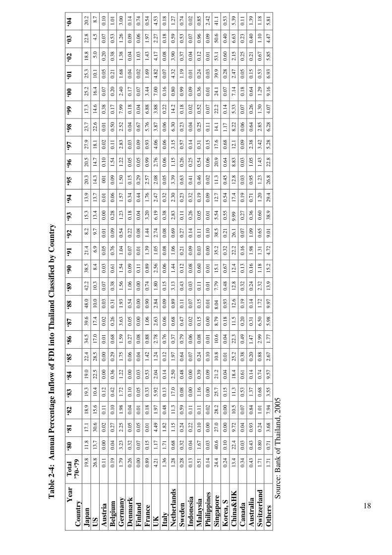
18
Tab
le 2
-4:
An
nu
al
Per
cen
tage
Infl
ow
of
FD
I in
to T
hail
an
d C
lass
ifie
d b
y C
ou
ntr
y
Y
ear
Cou
ntr
y
To
tal
’70
-‘7
9
‘80
‘8
1
‘82
‘8
3
‘84
‘8
5
‘86
‘8
7
‘88
‘8
9
‘90
‘9
1
‘92
‘9
3
‘94
‘9
5
‘96
‘9
7
‘98
‘9
9
‘00
‘0
1
‘02
‘0
3
‘04
Jap
an
1
9.8
1
1.8
1
7.1
1
8.9
1
9.3
1
9.0
2
2.4
3
4.5
3
9.6
4
8.0
4
2.2
3
8.5
2
1.4
8
.2
15.3
1
3.9
2
0.3
2
0.5
2
7.9
2
3.7
1
7.3
2
5.2
2
5.3
1
8.8
2
2.8
2
0.2
US
2
6.8
1
3.7
3
0.6
1
5.6
1
0.4
2
2.5
2
8.5
1
7.0
1
7.4
1
0.0
1
0.3
8
.4
6.9
9
.7
13.4
1
3.7
1
4.3
1
4.7
1
8.1
2
2.6
1
4.6
1
6.4
1
0.1
5
.0
4.5
8
.7
Au
stri
a
0.1
1
0.0
0
0.0
2
0.1
1
0.1
2
0.0
0
0.0
0
0.0
1
0.0
2
0.0
3
0.0
7
0.0
3
0.0
5
0.0
1
0.0
0
0.0
1
001
0
.10
0
.02
0
.01
0
.38
0
.07
0
.05
0
.20
0
.07
0
.10
Bel
giu
m
0.1
9
0.0
4
0.2
7
0.1
0
0.4
2
0.3
6
0.2
9
0.6
8
0.2
6
0.3
1
0.3
8
0.6
1
0.7
6
0.0
9
0.2
8
0.0
6
0.0
9
1.5
4
0.1
1
0.5
0
0.1
7
0.2
0
0.2
1
0.3
8
0.5
3
1.0
1
Ger
man
y
1.7
9
3.2
3
2.2
5
1.9
8
1.7
2
1.2
2
1.7
5
1.5
9
3.6
3
1.9
3
1.5
6
1.5
4
1.0
4
0.5
4
1.2
3
1.5
7
1.5
0
1.2
2
2.8
3
2.5
2
7.9
9
2.4
0
1.6
8
1.3
8
1.2
6
3.0
0
Den
mark
0
.26
0
.32
0
.05
0
.04
0
.10
0
.00
0
.06
0
.27
0
.05
0
.54
1
.06
0
.09
0
.07
0
.22
0
.18
0
.34
0
.15
0
.05
0
.03
0
.04
0
.18
0
.17
0
.04
0
.04
0
.09
0
.14
Fin
lan
d
0.0
0
0.0
7
0.0
5
0.0
1
0.0
5
0.0
3
0.0
4
0.0
8
0.0
0
0.0
0
0.0
0
0.1
1
0.0
1
0.0
8
0.0
4
0.4
4
0.2
9
0.0
5
0.0
9
0.6
7
0.0
4
0.0
7
0.0
2
1.0
3
0.0
6
0.7
4
Fra
nce
0
.89
0
.15
0
.01
0
.18
0
.33
0
.53
1
.42
0
.88
1
.06
0
.90
0
.74
0
.89
1
.39
1
.44
3
.20
1
.76
2
.57
0
.99
0
.93
5
.76
6
.88
3
.44
1
.69
1
.43
1
.97
0
.54
UK
4
.21
1
.17
4
.49
1
.97
5
.92
2
.04
1
.24
2
.78
2
.63
2
.84
1
.80
2
.56
1
.05
2
.74
6
.19
2
.47
2
.08
2
.76
4
.06
3
.87
3
.88
7
.00
4
.82
4
.17
2
.27
4
.53
Italy
1
.36
1
.71
1
.82
0
.48
0
.13
0
.14
0
.12
0
.76
0
.06
0
.09
0
.15
0
.06
0
.08
0
.08
0
.38
0
.32
0
.05
0
.06
0
.06
0
.06
0
.22
0
.16
0
.07
0
.08
0
.18
0
.18
Net
her
lan
ds
1.2
8
0.6
8
1.1
5
11.3
1
7.0
2
.50
1
.97
0
.37
0
.68
0
.89
3
.13
1
.44
1
.06
0
.69
2
.83
2
.30
3
.39
1
.15
3
.15
6
.30
1
4.2
0
.80
4
.32
3
.90
0
.59
1
.27
Sw
eden
0
.28
0
.32
0
.24
0
.59
0
.08
0
.48
0
.64
0
.79
0
.47
0
.11
0
.43
0
.12
0
.21
0
.27
0
.11
0
.23
0
.63
0
.26
0
.57
0
.23
0
.18
0
.99
1
.19
0
.37
0
.53
0
.74
Ind
on
esia
0
.13
0
.04
0
.22
0
.11
0
.00
0
.00
0
.07
0
.06
0
.02
0
.07
0
.03
0
.08
0
.09
0
.14
0
.26
0
.32
0
.41
0
.25
0
.14
0
.04
0
.02
0
.09
0
.01
0
.04
0
.07
0
.02
Mala
ysi
a
0.5
1
1.6
7
0.1
0
0.1
1
1.1
6
0.3
9
0.2
4
0.0
8
0.1
5
0.1
5
0.1
1
0.6
0
0.0
3
0.1
1
0.0
5
0.1
9
0.4
6
0.5
4
0.3
1
0.2
5
0.5
2
0.3
6
0.2
4
0.1
2
0.9
6
0.8
5
Ph
ilip
pin
es
0.1
4
0.0
3
0.0
0
0.0
2
0.0
0
0.0
9
0.1
0
0.0
1
0.0
0
0.0
1
0.0
1
0.0
1
0.0
0
0.1
0
0.0
1
0.0
9
0.0
2
0.0
6
0.1
5
0.1
1
0.0
7
0.0
1
0.0
3
0.0
1
0.0
9
2.4
2
Sin
gap
ore
2
4.4
4
0.6
2
7.0
2
8.2
2
5.7
2
1.2
1
0.8
1
0.6
8
.79
8
.04
7
.79
1
5.1
3
5.2
3
8.5
5
.54
1
2.7
1
1.3
2
0.9
1
7.6
1
4.1
2
2.2
2
4.1
3
9.9
5
3.1
5
0.6
4
1.1
Kore
a, S
0
.24
0
.10
0
.00
0
.00
0
.15
0
.04
0
.01
0
.04
0
.18
0
.93
0
.48
0
.67
0
.32
0
.21
0
.55
0
.54
0
.45
0
.64
0
.68
1
.17
0
.14
0
.07
0
.28
0
.60
0
.40
0
.53
Ch
ina&
HK
1
3.4
2
2.4
9
.72
1
0.5
1
1.3
1
8.4
2
5.2
2
2.3
1
1.5
1
2.6
1
2.8
1
2.4
2
2.2
2
6.1
9
.99
1
7.4
1
2.8
8
.83
1
2.1
8
.22
5
.33
7
.14
2
.47
2
.15
6
.63
5
.39
Can
ad
a
0.3
4
0.0
3
0.0
4
0.0
7
0.5
3
0.6
1
0.3
8
0.4
9
0.2
0
0.1
9
0.3
2
0.1
3
0.1
6
0.0
7
0.2
7
0.1
9
0.0
3
0.0
3
0.0
9
0.0
6
0.0
7
0.1
8
0.0
5
0.2
5
0.2
3
0.1
1
Au
stra
lia
0.4
3
0.4
3
0.9
3
0.8
4
1.3
7
0.1
4
0.2
0
1.4
7
0.3
1
0.1
4
0.2
4
0.1
6
1.9
8
1.0
9
0.3
6
0.7
1
0.9
5
1.0
5
2.3
8
0.6
4
0.2
6
0.6
4
0.1
5
0.2
1
0.4
0
1.3
9
Sw
itze
rlan
d
1.7
1
0.8
0
0.2
4
1.0
1
0.6
8
0.7
4
0.8
8
2.9
9
6.5
0
1.7
2
2.3
2
1.1
8
1.3
1
0.6
5
0.6
0
1.2
0
1.2
3
1.4
3
3.4
2
2.8
5
1.3
0
1.2
9
0.5
3
0.6
7
1.1
0
1.1
8
Oth
ers
1.7
1
0.7
1
3.6
8
7.9
4
3.5
5
9.5
7
2.6
7
1.7
7
5.9
8
9.9
7
13.9
1
5.2
4
.72
9
.01
3
8.9
2
9.4
2
6.8
2
2.8
5
.28
6
.28
4
.07
9
.16
6
.93
5
.85
4
.47
5
.81
Sourc
e: B
ank o
f T
hai
lan
d, 2005
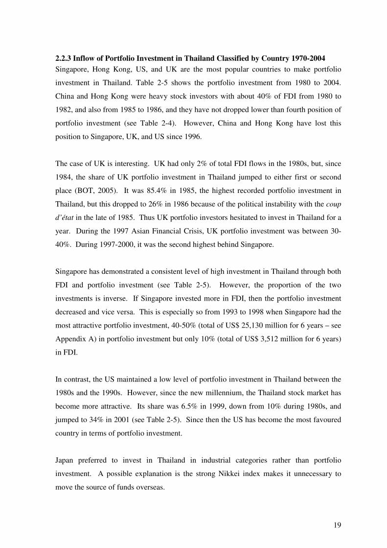
19
2.2.3 Inflow of Portfolio Investment in Thailand Classified by Country 1970-2004
Singapore, Hong Kong, US, and UK are the most popular countries to make portfolio
investment in Thailand. Table 2-5 shows the portfolio investment from 1980 to 2004.
China and Hong Kong were heavy stock investors with about 40% of FDI from 1980 to
1982, and also from 1985 to 1986, and they have not dropped lower than fourth position of
portfolio investment (see Table 2-4). However, China and Hong Kong have lost this
position to Singapore, UK, and US since 1996.
The case of UK is interesting. UK had only 2% of total FDI flows in the 1980s, but, since
1984, the share of UK portfolio investment in Thailand jumped to either first or second
place (BOT, 2005). It was 85.4% in 1985, the highest recorded portfolio investment in
Thailand, but this dropped to 26% in 1986 because of the political instability with the coup
d’état in the late of 1985. Thus UK portfolio investors hesitated to invest in Thailand for a
year. During the 1997 Asian Financial Crisis, UK portfolio investment was between 30-
40%. During 1997-2000, it was the second highest behind Singapore.
Singapore has demonstrated a consistent level of high investment in Thailand through both
FDI and portfolio investment (see Table 2-5). However, the proportion of the two
investments is inverse. If Singapore invested more in FDI, then the portfolio investment
decreased and vice versa. This is especially so from 1993 to 1998 when Singapore had the
most attractive portfolio investment, 40-50% (total of US$ 25,130 million for 6 years – see
Appendix A) in portfolio investment but only 10% (total of US$ 3,512 million for 6 years)
in FDI.
In contrast, the US maintained a low level of portfolio investment in Thailand between the
1980s and the 1990s. However, since the new millennium, the Thailand stock market has
become more attractive. Its share was 6.5% in 1999, down from 10% during 1980s, and
jumped to 34% in 2001 (see Table 2-5). Since then the US has become the most favoured
country in terms of portfolio investment.
Japan preferred to invest in Thailand in industrial categories rather than portfolio
investment. A possible explanation is the strong Nikkei index makes it unnecessary to
move the source of funds overseas.
20
Tab
le 2
-5:
An
nu
al
Per
cen
tage
Infl
ow
of
Port
foli
o I
nves
tmen
t (E
qu
ity S
ecu
riti
es)
into
Th
ail
an
d C
lass
ifie
d b
y C
ou
ntr
y
Y
ear
Cou
ntr
y
To
tal
’70
-‘7
9
‘80
‘8
1
‘82
‘8
3
‘84
‘8
5
‘86
‘8
7
‘88
‘8
9
‘90
‘9
1
‘92
‘9
3
‘94
‘9
5
‘96
‘9
7
‘98
‘9
9
‘00
‘0
1
‘02
‘0
3
‘04
Jap
an
6
.76
1
.41
2
.08
0
.15
0
.60
1
.98
0
.43
0
.18
1
.48
4
.99
0
.82
2
.12
0
.47
0
.04
0
.32
0
.85
0
.79
0
.36
0
.46
0
.21
0
.14
0
.42
1
.61
0
.07
0
.75
0
.16
US
1
4.7
1
0.6
3
9.2
1
.97
2
.29
1
.95
1
.36
1
7.0
7
.07
1
1.0
3
.44
6
.90
5
.56
5
.68
3
.53
8
.82
5
.17
5
.76
7
.35
1
4.1
6
.51
1
3.0
3
4.1
2
6.8
4
4.3
4
4.6
Au
stri
a
0.0
2
0.0
0
9.7
1
6.5
4
0.0
0
0.0
0
0.0
1
0.0
0
0.0
0
0.0
0
0.0
0
0.0
0
0.0
0
0.0
0
0.0
0
0.0
0
0.0
2
0.0
0
0.0
0
0.0
0
0.0
0
0.0
8
0.6
0
0.0
0
0.0
0
0.0
0
Bel
giu
m
0.0
1
0.0
0
0.0
0
0.0
0
0.0
2
0.0
0
0.0
0
0.0
0
0.0
1
1.2
2
0.1
8
0.2
6
0.0
2
0.0
1
0.0
0
0.2
4
0.5
5
1.6
8
1.5
1
4.1
9
1.6
8
12.0
2
.82
0
.61
1
2.7
0
.12
Ger
man
y
1.0
6
0.0
5
0.6
5
1.8
0
1.3
8
1.0
5
0.0
5
0.1
2
0.1
5
0.0
3
0.1
0
0.1
3
0.1
0
0.1
0
0.0
1
0.0
5
0.2
4
0.1
2
0.2
3
0.5
8
0.0
0
3.2
7
0.0
0
0.0
0
0.0
5
0.0
2
Den
mark
0
.02
0
.00
0
.00
0
.00
0
.00
0
.00
0
.00
0
.00
0
.00
0
.00
0
.04
0
.00
0
.01
0
.00
0
.00
0
.00
0
.00
0
.00
0
.04
0
.00
0
.00
0
.00
0
.00
0
.00
0
.05
0
.00
Fin
lan
d
0.0
0
0.0
0
0.0
0
0.0
0
0.0
0
0.0
0
0.0
0
0.0
0
0.0
0
0.0
0
0.0
0
0.0
0
0.0
0
0.0
0
0.0
0
0.0
0
0.0
0
0.0
0
0.0
0
0.0
1
0.0
0
0.0
0
0.0
0
0.0
0
0.0
0
0.0
0
Fra
nce
0
.42
0
.01
0
.70
0
.02
0
.00
0
.25
0
.09
0
.03
0
.01
0
.00
0
.74
0
.41
0
.11
0
.00
0
.03
0
.17
0
.09
0
.72
0
.23
0
.33
1
.29
0
.27
0
.80
0
.07
0
.10
0
.35
UK
1
.23
0
.01
1
.75
0
.10
0
.05
2
7.8
8
5.4
2
6.0
2
5.4
3
6.0
3
1.0
2
3.9
2
2.9
1
6.1
2
6.1
2
3.9
2
0.4
2
7.9
3
5.2
3
1.2
4
0.8
4
1.0
2
3.8
1
8.4
1
4.7
2
4.6
Italy
0
.00
0.0
0
0.0
0
0.0
0
0.0
0
0.0
0
0.0
0
0.0
0
0.0
0
0.0
0
0.0
0
0.0
0
0.0
0
0.0
0
0.0
0
0.0
0
0.0
0
0.0
0
0.0
1
0.0
0
0.0
0
0.0
0
0.0
0
0.0
0
0.0
0
0.0
2
Net
her
lan
ds
2.7
7
0.0
0
0.0
0
0.0
0
0.0
0
0.0
0
0.0
1
0.0
9
0.0
1
1.2
4
1.4
4
3.5
6
8.5
9
6.6
9
0.0
6
0.0
5
0.2
3
0.3
1
0.0
7
0.2
4
1.3
8
0.1
4
0.4
7
1.2
2
0.1
8
0.2
4
Sw
eden
0
.00
0
.00
0.0
0
0.0
0
0.0
0
0.0
0
0.0
0
0.0
0
0.0
0
0.0
0
0.0
1
0.0
4
0.0
1
0.0
0
0.0
0
0.0
5
0.0
0
0.0
0
0.4
2
0.0
1
0.0
0
0.0
0
0.0
0
0.0
0
0.0
2
0.2
2
Ind
on
esia
0
.34
0
.48
0
.14
0
.65
0
.02
0
.00
0
.10
0
.00
0
.00
0
.02
0
.00
0
.01
0
.01
0
.00
0
.03
0
.00
0
.00
0
.01
0
.19
0
.18
0
.07
0
.00
0
.13
0
.00
0
.02
0
.00
Mala
ysi
a
0.8
4
0.3
3
0.1
1
0.4
7
0.0
0
0.0
3
0.0
7
0.0
1
0.0
7
0.0
4
0.0
9
0.2
8
0.0
3
0.0
2
0.0
0
0.0
9
0.0
6
0.0
2
0.0
1
0.0
4
0.0
0
0.0
0
0.0
0
0.0
0
0.0
2
0.0
6
Ph
ilip
pin
es
0.0
1
0.0
0
0.1
4
0.0
0
0.0
0
0.0
2
0.0
1
0.0
0
0.0
1
0.0
0
0.0
0
0.0
0
0.0
0
0.1
0
0.0
0
0.1
2
0.0
0
0.0
0
0.0
2
0.0
0
0.0
7
0.0
0
0.0
0
0.0
0
0.0
0
0.0
2
Sin
gap
ore
1
.48
1
9.8
1
.88
0
.75
7
3.3
3
.44
1
.84
1
1.5
1
4.8
3
6.7
3
7.0
4
1.6
4
0.3
3
2.4
4
9.6
4
1.9
5
1.7
4
8.5
4
2.2
3
9.6
1
7.3
1
8.9
2
2.5
1
9.6
8
.84
8
.65
Kore
a, S
0
.01
0
.00
0
.00
0
.00
0
.00
0
.00
0
.00
0
.00
0
.02
0
.00
0
.01
0
.00
0
.00
0
.03
0
.00
0
.00
0
.02
0
.01
0
.00
0
.00
0.0
0
0.0
0
0.0
0
0.0
0
0.0
0
0.0
0
Ch
ina&
HK
2
6.1
6
1.1
4
3.4
8
4.2
1
2.9
1
5.7
9
.35
4
3.3
5
0.1
7
.4
21.4
1
4.0
1
9.4
3
4.6
1
7.8
1
9.2
1
6.7
1
1.6
1
1.1
7
.62
2
9.2
4
.47
3
.75
7
.40
1
0.1
7
.52
Can
ad
a
0.0
4
0.0
0
0.0
0
2.5
7
0.7
1
0.0
1
0.0
7
0.0
0
0.0
0
0.0
1
0.0
1
0.0
8
0.0
8
0.6
1
0.6
3
1.0
5
0.0
3
0.0
1
0.0
1
0.0
1
0.0
0
0.0
9
0.1
3
0.0
0
0.0
0
0.0
0
Au
stra
lia
0.1
7
0.0
1
0.0
0
0.0
0
0.0
0
0.0
1
1.1
4
0.2
8
0.0
5
0.3
2
1.1
0
0.4
0
0.0
1
0.0
4
0.2
0
0.0
9
1.3
1
0.4
4
0.1
1
0.0
4
0.0
2
0.0
9
3.4
2
0.0
0
0.3
5
1.2
4
Sw
itze
rlan
d
1.0
4
0.0
7
0.3
6
0.3
7
0.0
7
0.0
6
0.0
2
0.7
6
0.2
9
0.0
5
0.5
1
0.8
4
0.1
8
0.2
2
0.1
5
0.4
7
1.6
2
1.1
2
0.3
9
0.3
0
0.0
6
0.2
3
0.5
4
0.6
1
1.7
9
1.4
2
Oth
ers
43.0
6
.21
0
.00
0
.36
8
.72
4
7.7
0
.15
0
.75
0
.56
1
.05
2
.09
5
.52
0
.13
3
.24
1
.50
2
.87
1
.06
1
.38
0
.62
1
.40
1
.54
6
.13
5
.30
2
5.0
6
.01
1
0.8
Sourc
e: B
ank o
f T
hai
lan
d, 2005
21
2.3 The Development of FDI Policy in Thailand
1940s-1950s State capitalism
The country became a state monopoly for most imports and exports.
1958-71 Import substitution
The first Economic Development Plan (1961-66) brought a reduction in direct government
involvement in the economy and greater promotion of private investment. The import
substitution policy was introduced with a high level of protection and tariffs especially on
consumer products (Tangkitvanich et al., 2004). The Board of Investment (BOI)
established the tax concession and the Industrial Promotion Act of 1960. Tariff structures
were revised several times to give better protection to domestic industries. Balance of
payments problems led to a discussion of sustainability of import substitution policy.
1972-1992 Export promotion
The third Economic Development Plan (1972-76) introduced export promotion. These
included: the investment law amended in 1972 which provided exemptions from duty on
raw materials and intermediate items for exporting industries; Alien Business Law of 1972
which prohibited foreigners from entering several business areas; investment zones (21 of
72 provinces) were designated; the Investment Promotion Act was enacted in 1977,
introducing income tax holidays and a 50% concessionary import duty on machinery; and
tax incentives on raw materials and machinery were reduced for Bangkok and its
perimeter, to promote deeper industrial decentralization (BOI, 2005). The investment
Promotion Act was amended in 1987, introduced tax privileges and refunds, industrial
zones, and export-processing zones; and the sixth Economic Development Plan (1987-91)
was planned to improve income distribution and reduce income disparity.
1993-1996 Promotion of industrial decentralization
The seventh Economic Development Plan (1992-96) aimed to reduce the income disparity
between urban and rural areas (NESDB, 2004). This included setting up the promotion of
sustainable development; the Investment Promotion Act was amended in 1993 to promote
industrial decentralization, with generous incentives provided to encourage industries to
locate in the rural areas.
22
1997-present Post-crisis liberalization
After the 1997 Asian Financial Crisis, liberalization was extended as part of the IMF-led
reform package and included: the Foreign Business Act of 1999, allowing full foreign
participation in most manufacturing sectors; Condominium Act was amended in 1998 to
allow foreigners to wholly own buildings on two acres or less of land; the Corporate Debt
Restructuring Advisory Committee was established to supervise and accelerate debt
restructuring; ASEAN Investment Agreement (AIA) was adopted in 1998; Bankruptcy Act
was amended in 1999 to establish a central bankruptcy court; local content requirements
were eliminated for vehicle assembly in 1999, and foreigners were allowed to own 100%
of shares in promoted manufacturing projects in 2000 (NESDB, 2004).
2.4 Impact of Investment Policy on FDI in Thailand
Thailand’s investment policy regime has been continually revised to reflect the
development of the overall economy in general and, in particular, from the era of import
substitution to export promotion and post the 1997 Asian Financial Crisis liberalisation.
Investment policy has become much more liberal during the past decade. The changes in
investment policies have an impact on the location of FDI while changes in the direction of
greater openness allowed firms to set themselves up in a particular location, but do not
guarantee that they will do so. In contrast, changes in the direction of less openness will
ensure a reduction in FDI (Mallampally and Sauvant, 1999). The investment policies
should enable the country to support a more competitive environment with alternative
strategies for the country to maximize the productivity benefits from FDI.
The Board of Investment (BOI) was set up to develop a plan to attract foreign investment
from overseas and to collaborate to boost bargaining power and proceed faster in
approaching potential sources of investment. The principal aim is to further the
development of FDI strategies of the Thai government. This included the first National
Economic Development Plan by the National Economic and Social Development Board
(NESDB) in 1961 with the import substitution regime to promote industrialization
(Kohpaiboon, 2003). In addition, the Ninth National Economic and Social Development
Plan (2002-2006) was established to enhance investment strategies such as preparing
immediate measures to alleviate drought, prevent any increase in non-performing loans,
launching offensive strategies to support Thai exports, accelerating economic stimulation
packages and strengthening the local economy to attract new or reinvested FDI.
23
2.5 Summary
In the early stage of FDI development in Thailand, US and Japan were the main sources of
inflows of FDI into the country, which accounted for at least 50% of all FDI inflows. The
inflows of FDI into Thailand started to increase rapidly in the mid of 1980s because of the
effect of “Endaka”, which is an appreciation of Japanese Yen against the US Dollar.
Therefore, Japanese investors shifted their funds to invest overseas in order to reduce the
production costs and to gain more competitive advantage from the low labour cost
countries with rich natural resources. Japanese manufacturers had started to become major
foreign investors in many countries, including Thailand.
The inflows of portfolio investment into Thailand started to increase dramatically in the
mid 1980s at the same time as Japanese and US investment in FDI. Singapore and Hong
Kong are the main sources of portfolio investment fund into Thailand, followed by the US
and the UK.
In addition, Thailand has developed its FDI policy since 1940s and promoted FDI policy
from import-substitution to export-oriented in the 1980s. This is not only to improve the
growth of the economy but to increase the country’s welfare.
The following chapter provides the background of FDI theory and introduces the
applications of the FDI theory.
CHAPTER 3
FOREIGN DIRECT INVESTMENT THEORIES
This chapter reviews the relevant literature that focuses on both the firm and the aggregate
level of FDI under three main FDI theories: the Eclectic Paradigm concept, the Resource-
Based Theory, and the Business Network Theory. This chapter also discusses issues
concerning FDI. An overview of the FDI literature is discussed first followed by a
discussion of FDI relationships, specifically the impact between the government and the
investment policy.
The chapter consists of five sections. The first section provides an overview of the FDI
theories. The second section provides an overview of the Eclectic Paradigm concept
followed by the Resource-Based Theory and the main Business Network Theory of FDI.
Section five summarizes the chapter.
3.1 Foreign Direct Investment
3.1.1 An Overview and Application of FDI Theory
Foreign investments flow to host countries because of lower production costs. As foreign
investors search for the location that will provide the highest returns on their investment,
they look for countries with abundant natural resources but low-quality institutions. Some
countries such as Thailand and Indonesia encourage FDI or Foreign Indirect Investment
(FII) to their countries with friendly regulations offering them a higher rate of return. The
popular determinants of FDI flowing to smaller economies include market potential and
low relative unit labour cost which have significant and plausible effects enhancing FDI
decision-making (Carstensen and Toubal, 2004; Cheng and Kwan, 2000; Noorbakhsh and
Paloni, 2001). For example, Hong Kong and Singapore have mainly targeted the financial
category, which is relatively skill intensive. In Korea, most of the FDI was invested in the
manufacturing category. Thailand attracted a quarter of FDI flows in the capital-intensive
and relative skill-intensive chemical, machinery and electrical manufacturing sectors
(Velde and Morrissey, 2002).
Following the Second World War, global FDI was dominated by the US, as much of the
world recovered from the devastation of the war. The US accounted for around three
25
quarters of new FDI between 1945 and 1960. Since then, FDI has spread to become a
global phenomenon. At the same time, numerous researchers have conducted studies on
FDI, including investigating the fundamental theories of FDI, various macro economic
variables that influence FDI, the impact of economic integration on the movement of FDI,
and the advantages and disadvantages of FDI in the host countries (Carstensen and Toubal,
2004; Cheng and Kwan, 2000; Zhang, 2001a). Dunning (1980) introduced the FDI theory
via the Eclectic Paradigm. Accordingly, the Eclectic Paradigm shows that specific
advantages related to a firm or its country of origin can be estimated as independent
variables in an equation to describe the origins of FDI in a host country. Most originators
agree that there exists a positive causal relationship between FDI and economic
performance, either in the short run or the long run, or both. Firms from developing
countries face immense difficulties in setting up a distribution network, keeping in close
touch with the rapid changes in a consumer-taste, mastering the technicalities of industrial
norms and safety standards, and building up a new product image. Their lack of skills
constitutes a key entry barrier to markets (Blomström and Kokko, 1997); therefore, they
seek Multinational Enterprises (MNEs) to compensate for the deficiencies.
Perlmutter (1969) introduced FDI as a strategic alternative that firms adopt to serve foreign
markets after they have gained international experience through trade and/or licensing.
The potential benefits of FDI to host countries from encouraging capital inflows include:
(1) foreign firms bring superior technology; (2) foreign investment increases competition
in the host country; (3) foreign investment typically results in increased domestic
investment; (4) foreign investment gives advantages in terms of export market; and (5)
foreign investment can aid in bridging a host country’s foreign exchange gap (Brooks et
al., 2003). These may lure the government of host countries to rapidly transform from
agricultural production and the exploitation of raw materials into major producers and
exporters of manufactured goods.
To examine the potential benefit of FDI in host countries, Ismail and Yussof (2003) used
time series data on FDI, wages, labour force, skills, R&D expenditure, and the interest rate
to analyse the FDI impact on economic development. Their study showed the labour
market determinants differ between countries such as Malaysia, Thailand, and the
Philippines in terms of the FDI role in the country. Their results suggested that, with
regard to labour market competitiveness, different countries may require different policy
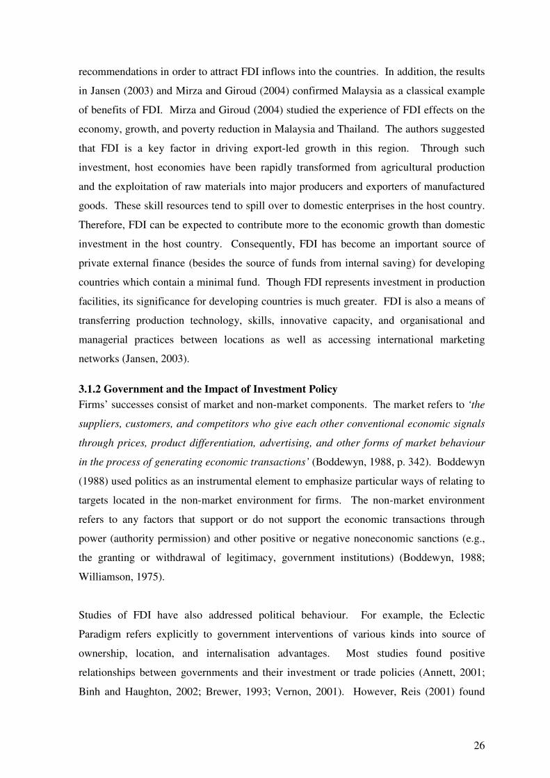
26
recommendations in order to attract FDI inflows into the countries. In addition, the results
in Jansen (2003) and Mirza and Giroud (2004) confirmed Malaysia as a classical example
of benefits of FDI. Mirza and Giroud (2004) studied the experience of FDI effects on the
economy, growth, and poverty reduction in Malaysia and Thailand. The authors suggested
that FDI is a key factor in driving export-led growth in this region. Through such
investment, host economies have been rapidly transformed from agricultural production
and the exploitation of raw materials into major producers and exporters of manufactured
goods. These skill resources tend to spill over to domestic enterprises in the host country.
Therefore, FDI can be expected to contribute more to the economic growth than domestic
investment in the host country. Consequently, FDI has become an important source of
private external finance (besides the source of funds from internal saving) for developing
countries which contain a minimal fund. Though FDI represents investment in production
facilities, its significance for developing countries is much greater. FDI is also a means of
transferring production technology, skills, innovative capacity, and organisational and
managerial practices between locations as well as accessing international marketing
networks (Jansen, 2003).
3.1.2 Government and the Impact of Investment Policy
Firms’ successes consist of market and non-market components. The market refers to ‘the
suppliers, customers, and competitors who give each other conventional economic signals
through prices, product differentiation, advertising, and other forms of market behaviour
in the process of generating economic transactions’ (Boddewyn, 1988, p. 342). Boddewyn
(1988) used politics as an instrumental element to emphasize particular ways of relating to
targets located in the non-market environment for firms. The non-market environment
refers to any factors that support or do not support the economic transactions through
power (authority permission) and other positive or negative noneconomic sanctions (e.g.,
the granting or withdrawal of legitimacy, government institutions) (Boddewyn, 1988;
Williamson, 1975).
Studies of FDI have also addressed political behaviour. For example, the Eclectic
Paradigm refers explicitly to government interventions of various kinds into source of
ownership, location, and internalisation advantages. Most studies found positive
relationships between governments and their investment or trade policies (Annett, 2001;
Binh and Haughton, 2002; Brewer, 1993; Vernon, 2001). However, Reis (2001) found
27
different opinions of policy relevance and FDI by measuring the welfare effect on FDI.
Reis argued that producers in the host country will no longer be able to invest in the R&D
sector after the opening of the economy to FDI, which has a negative effect on national
income and profits.
Boddewyn (1988) enriched the Eclectic Paradigm by explicitly incorporating political
elements in the consideration of ownership, internalisation, and location advantages. The
author largely focused on government as the target of political behaviour. The author
stated that Dunning’s Eclectic Paradigm can be readily expanded to include the political
element in its consideration of firm-specific, location, and internalisation advantages.
Boddewyn’s results conclude that all advantages are necessary for FDI, “such as market
imperfections may also be enacted through political behaviour in order to raise the
transaction costs of competitors and to exploit various rents arising from these
imperfections” (Boddewyn, 1988, p. 357).
The international theory of FDI includes government policies that create market
imperfections, which makes FDI an economically reasonable strategic alternative for firms.
For example, Brewer (1993) examined the effects of government policies on market
imperfections and FDI. Brewer suggested that government policies are significant
determinants of the sizes and growth rates for markets of all goods and services in the
economy. Vernon (2001) focused on government regulation and how government can
reshape the policy in a global economy for the firms. The area of FDI and government
policies has become more popular in the later studies.
Haddad and Harrison (1993) explained that the benefits from FDI, such as transferring
technology to domestic firms, are not equally distributed in developing countries.
Solicitous policies (income tax holidays and import duty exemptions) should be developed
to avoid inequality among big and smaller cities, to encourage efficiency of domestic
firms, to benefit from linkages with and spillovers from foreign firms, and to attract FDI
around the country. Other research findings show the dispersal of productivity is less in
those sectors with more foreign firms and that foreign investors may be attracted to protect
domestic markets rather than transferring technology to domestic firms (Binh and
Haughton, 2002).
28
Annett (2001) developed the concept of government budget and policy by adding the
social fractionalisation of a country’s population (ethno-linguistic and religious dimension)
to explore the relationship between the political instability and government consumption.
The author found that higher fractionalisation led to political instability. Annett showed a
strong positive relationship between fractionalisation and government consumption.
Furthermore, the author also showed the effect of fractionalisation on government
consumption operates through the political instability channel.
In the case of the impact of FDI on home and host countries, Sanna-Randaccio (2002)
studied the welfare effect when taking into account the FDI effect, not only in product
market competition, but also its influence on the incentive to innovate and on the firms’
overall technological level. The author showed that, in high technology sectors, a policy of
attracting FDI may increase welfare in both home and host countries. Further, the results
indicated that there is a possibility that FDI will increase the host-country welfare with the
technology transfer. Welfare in the host country will benefit more if technological
spillovers are at national level instead of international level.
FDI does not always increase welfare in the host country, especially if firms have
monopoly power in the world market. These firms can increase output from the new
competition by lowering the price of the exportable, thus reducing the terms of trade and
lowering welfare in the host country. Reis (2001) studied the welfare effect of foreign
investment and found that foreign investors are able to introduce new goods into the
economy at a lower cost than nationals. This implies that after the opening of the economy
to foreign investors, indigenous producers find that it is not profitable to invest in the R&D
sector. This has a negative effect on national income and the impact of FDI, which is
translated into loss of profits. Furthermore, foreign investment may decrease national
welfare due to the transfer of profits to the home country, even when the increase in the
rate of growth has a positive effect on welfare; this occurs only if the increase in
productivity is great enough to compensate for the loss of profits. Moreover, Reis
suggested that the policy relevance of the theoretical results should not focus only on their
quantitative importance.
Milner et al. (2004) investigated the effects of Japanese firms (home country) and Thailand
(host country) characteristics on the inter-industry pattern of FDI at the firm level. The
29
authors found strong evidence to support the fact that Thai government incentives have
important effects on the cross-industry pattern on FDI, which was similar to results found
in Jiang’s study (Jiang, 2003). Jiang studied the forces of FDI in China. Jiang’s results
suggested that the relatively stable political conditions in China had a strong positive
influence on FDI decisions. Low labour and establishment costs in China as well as
cultural factors were insignificant in deterring FDI. Jiang’s study demonstrated that the
incentives provided by the Chinese government would most likely be treated as additional
benefits by most international firms, rather than as decisive factors in their FDI decision
making. Jiang’s findings supported previous studies by Hartman (1984), Head et al.
(1999), and Simmons (2003).
The above literature suggests several preliminary conclusions about the role of government
policies in FDI. There is recognition that government policies are important determinants
of FDI. However, according to Reis’s (2001) suggestion, the quality of residents’ life in
the host country should be included in future studies because quality is just as important as
quantity of FDI.
3.1.3 The Advantages of FDI Theory
In the early and mid seventies, the respective merits of various streams of economic
theories (capital, trade, location, and investment) and the beginning of the phenomenon of
international production occurred in two streams of the theory on international production
(Calvet, 1981; Hymer, 1972; Kim, 2000; Ragazzi, 1973). One is a micro-oriented theory,
which explains why firms choose the location of a particular value-added activity in
different host countries based on the absolute costs and benefits comparison (Dunning,
1976). The other stream is a macro-oriented theory, which explains the firms’ activities
are best undertaken in different host countries based on the comparative costs and benefits
(Dunning, 1976). Casson (1982) argued that the theory of FDI consists of three integrating
theories: the Theory of International Capital Markets, the Theory of the Firm, and the
Theory of Trade. The integration of all three theories provides answers to complicated
FDI issues. The Theory of International Capital Markets answers the issues of the origins
of finance (funding, risk-bearing including ownership and utilisation risks). The Theory of
the Firm clarifies the problems in the location of control such as country of
registration/origin, location of headquarters, cultural affiliation, and source of
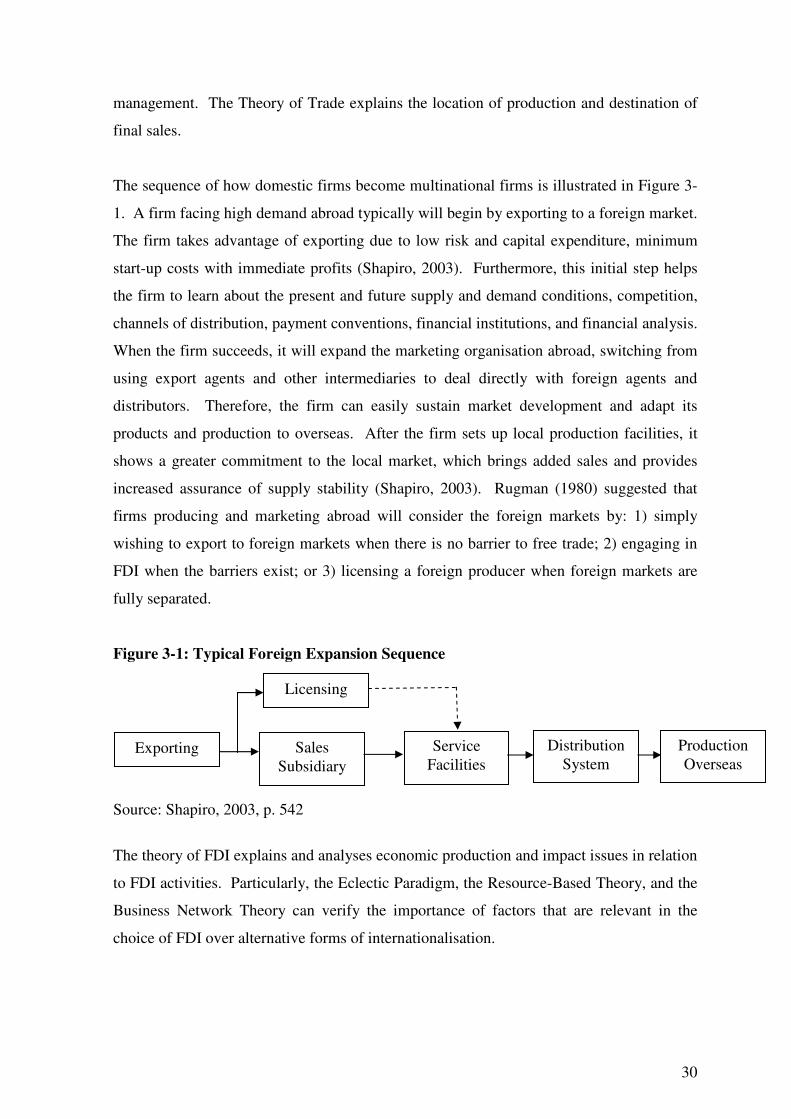
30
management. The Theory of Trade explains the location of production and destination of
final sales.
The sequence of how domestic firms become multinational firms is illustrated in Figure 3-
1. A firm facing high demand abroad typically will begin by exporting to a foreign market.
The firm takes advantage of exporting due to low risk and capital expenditure, minimum
start-up costs with immediate profits (Shapiro, 2003). Furthermore, this initial step helps
the firm to learn about the present and future supply and demand conditions, competition,
channels of distribution, payment conventions, financial institutions, and financial analysis.
When the firm succeeds, it will expand the marketing organisation abroad, switching from
using export agents and other intermediaries to deal directly with foreign agents and
distributors. Therefore, the firm can easily sustain market development and adapt its
products and production to overseas. After the firm sets up local production facilities, it
shows a greater commitment to the local market, which brings added sales and provides
increased assurance of supply stability (Shapiro, 2003). Rugman (1980) suggested that
firms producing and marketing abroad will consider the foreign markets by: 1) simply
wishing to export to foreign markets when there is no barrier to free trade; 2) engaging in
FDI when the barriers exist; or 3) licensing a foreign producer when foreign markets are
fully separated.
Figure 3-1: Typical Foreign Expansion Sequence
Source: Shapiro, 2003, p. 542
The theory of FDI explains and analyses economic production and impact issues in relation
to FDI activities. Particularly, the Eclectic Paradigm, the Resource-Based Theory, and the
Business Network Theory can verify the importance of factors that are relevant in the
choice of FDI over alternative forms of internationalisation.
Licensing
Exporting Sales Subsidiary
Service Facilities
Distribution System
Production Overseas
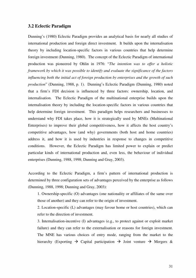
31
3.2 Eclectic Paradigm
Dunning’s (1980) Eclectic Paradigm provides an analytical basis for nearly all studies of
international production and foreign direct investment. It builds upon the internalisation
theory by including location-specific factors in various countries that help determine
foreign investment (Dunning, 1980). The concept of the Eclectic Paradigm of international
production was pioneered by Ohlin in 1976: “The intention was to offer a holistic
framework by which it was possible to identify and evaluate the significance of the factors
influencing both the initial act of foreign production by enterprises and the growth of such
production” (Dunning, 1988, p. 1). Dunning’s Eclectic Paradigm (Dunning, 1980) noted
that a firm’s FDI decision is influenced by three factors: ownership, location, and
internalisation. The Eclectic Paradigm of the multinational enterprise builds upon the
internalisation theory by including the location-specific factors in various countries that
help determine foreign investment. This paradigm helps researchers and businesses to
understand why FDI takes place, how it is strategically used by MNEs (Multinational
Enterprises) to improve their global competitiveness, how it affects the host country’s
competitive advantages, how (and why) governments (both host and home countries)
address it, and how it is used by industries in response to changes in competitive
conditions. However, the Eclectic Paradigm has limited power to explain or predict
particular kinds of international production and, even less, the behaviour of individual
enterprises (Dunning, 1988, 1998; Dunning and Gray, 2003).
According to the Eclectic Paradigm, a firm’s pattern of international production is
determined by three configuration sets of advantages perceived by the enterprise as follows
(Dunning, 1988, 1998; Dunning and Gray, 2003):
1. Ownership-specific (O) advantages (one nationality or affiliates of the same over
those of another) and they can refer to the origin of investment.
2. Location-specific (L) advantages (may favour home or host countries), which can
refer to the direction of investment.
3. Internalisation-incentive (I) advantages (e.g., to protect against or exploit market
failure) and they can refer to the externalisation or reasons for foreign investment.
The MNE has various choices of entry mode, ranging from the market to the
hierarchy (Exporting � Capital participation � Joint venture � Mergers &
32
Acquisition � Greenfield � Wholly owned subsidiary) (Brewer, 1993; Dunning,
1998).
Several studies have employed the Dunning’s paradigm (also called OLI Paradigm) to
identify the global strategic approaches of firms to other regions. Dunning’s paradigm
explains the preferences of firms, identifies the factors that affect FDI netflow, the impact
of FDI on economic growth and the technological advantages (see Agarwal and
Ramaswami, 1992; Ismail and Yussof, 2003; Loungani and Razin, 2001; Pak and Park,
2005).
Hill et al. (1990) studied the factors (such as strategic, environmental, and transaction) that
influence firms’ choice of entry mode into the foreign market (licensing or franchising,
entering into a joint venture, and setting up a wholly owned subsidiary) and integrated
factors within the framework of an Eclectic theory of choice of entry mode. In the Hill et
al. (1990) framework, each of the entry modes is consistent with a different level of
control, resource commitment, and dissemination risk. It can be explained as follows:
1. Entry mode and control. Different entry modes imply a different level of control
over the foreign operation. Calvet (1981) and Anderson and Gatignon (1986)
pointed out that different entry modes imply a different level of control, which is
lowest in the case of licensing and highest in the case of a wholly owned subsidiary,
over the foreign operation. Moreover, Eden and Lenway (2001) summarised the
forms of foreign investment and control level in the same way. However, in the case
of a joint venture, the level of control depends on the ownership split and the number
of parties involved.
2. Entry mode and resource commitment. According to Vernon’s (1966) study,
resource commitment assets cannot redeploy to alternative uses without cost. These
assets can be intangible (e.g., management know-how, technology) or tangible (e.g.,
physical plant, machinery). The level of resource commitment required for licensing
is low because the licensee bears most of the costs of opening up and serving the
foreign market. For the wholly owned subsidiary, it has to bear all costs, thus the
level of resource commitment is correspondingly high. The level of resource
33
commitment for a joint venture will fall between these two extremes, depending on
the ownership split and resource sharing between venture partners.
3. Entry mode and dissemination risk. The dissemination risk refers to the risk that
firm-specific advantages in know-how will be expropriated by the licensing or joint
venture partner. Technological and marketing know-how constitutes the basis of the
competitive advantage of many firms (Rugman, 1982). The risk of the dissemination
of know-how is likely to be lowest in the case of a wholly-owned subsidiary and
highest in the case of licensing.
Hill et al. (1990) discussed three factors: strategic (extent of national differences, extent of
scale economies, global concentration), environmental (country risk, location familiarity,
demand conditions, volatility of competition), and transaction cost consideration (value of
firm-specific know-how, tacit nature of know-how) with respect to the decision of entry
mode. They showed firms pursued a global strategy with a high-control entry mode
(wholly-owned subsidiaries) preference. However, when the country risk is high, licensing
and joint ventures were favoured over wholly-owned subsidiaries. According to the
transaction cost logic, if the reduction in transaction costs exceeds the costs of establishing
and transferring know-how, wholly-owned subsidiaries make more sense. The authors
concluded that management decision-makers should consider the relative weight of the
strategic, environmental, and transaction-specific factors into an eclectic theory to identify,
select, and influence the mode of entry.
Agarwal and Ramaswami (1992) examined the effect of interrelationships among a firm’s
ownership, location, and internalisation advantages on its choice of entry modes;
exporting, licensing, joint venture, and sole venture in foreign markets. The authors’
results showed the effects of the interrelationship, which implied that the firms would like
to establish a market presence in foreign countries through direct investment. However,
the firms’ abilities are constrained by their size and multinational experience. In addition,
firms used investment modes only in high potential markets.
Eicher and Kang (2005) examined multinationals’ optimal entry mode into foreign markets
as a function of market size, FDI fixed costs, tariffs, and transport costs. The authors
extended the Mueller (2001) structure to include international trade and transport costs to
34
investigate the dynamics of a three-stage entry mode between a local firm and its
multinational company (MNC) rival. The results varied with competition intensity in the
host country and were not different from previous research. It showed that low trade
barriers favoured international trade over other entry options on the part of MNCs. As
trade barriers increase, however, the authors found that trade depressed the price levels and
rendered it less likely that the MNCs could overcome trade barriers. FDI also existed in
markets due to the MNCs’ advantage in production cost over the local firm. High fixed
investment costs increased the threshold of market size for FDI, which cannot be offset
unless the trade barriers are sufficiently low to allow for MNCs’ export penetration. With
sufficiently high trade barriers, MNC favours acquisitions over trade as long as FDI fixed
costs are not too large to allow for FDI. Moreover, large markets give rise to acquisition
and independent trade barriers, because the monopoly power derived from acquisitions are
very attractive. In the case of high competition, FDI becomes the predominant entry mode,
which allows the MNCs’ to take full benefit of their ownership advantage.
Itaki (1991) critically dealt with the Eclectic theory of the multinational enterprise. He
examined the theoretical redundancy of the ownership advantage, the inseparability of the
ownership advantage from the location advantage, the conceptual ambiguity of the location
advantage, and possible methodological dangers of the multi-factor analysis under the
three headings (ownership, location, and internalisation) of the Eclectic theory.
Itaki argued that the ownership advantage consisted of the firm’s internal economies of
integration, internalized external economies, minimized transaction costs, and market
power. The author argued that Eclectic theory confused the ownership advantage in
engineering terms and ownership advantage is influenced by and inseparable from location
factors. The author suggested that the theory should distinguish between real terms and
nominal terms. Dunning (1988) agreed with Itaki’s criticism and accepted it to some
degree. Further, Boddewyn (1988) expanded Dunning’s model by explicitly incorporating
political elements such as ownership, internalisation, and location advantages and
commented about the possible contents of a broader MNE theory to explain FDI.
35
3.2.1 Applications of Eclectic Paradigm Concept
Chandprapalert (2000) explored the motives and determinants of the US FDI and
multinational enterprises’ activity in Thailand. The author looked at the role of ownership
advantage, location advantage, and internalisation advantage as defined in the Eclectic
Paradigm. Using primary data, the author empirically tested some of the determinants and
strategic motivations of FDI based on managerial perceptions. Linear regression was used
to analyse and test the correlation coefficient.
Chandprapalert’s (2000) study showed strong empirical evidence to support the importance
of ownership advantage, firm size, and multinational experience. It showed that larger
firms have greater ability to absorb losses than smaller firms, and have more financial
assets to invest overseas and, therefore, are less sensitive to uncertainty effects. In terms of
location advantage, the market potential was significant for Thailand and showed a strong
positive relationship between the market potential factor and US investment in Thailand.
There is strong empirical evidence in the literature for internalisation (Buckley and Casson,
1981; Rugman, 1986; Teece, 1981). However, Chandprapalert’s findings also showed a
strong negative relationship between investment risks (exchange rate fluctuation, taxes,
large public deficit, and institutional reform) and US FDI in Thailand.
Galan and Gonzalez-Benito (2001) studied 103 Spanish firms that have conducted FDI.
The FDI was built on the Eclectic Paradigm (ownership, location, and internalisation
factors), which affects the internationalisation processes of firms. The results showed the
important FDI determinants such as the existence of specific assets of an intangible
scenario. It also showed that the transaction costs and other questions related to
knowledge transfer were relevant in the choice of FDI over alternative forms of
internationalisation.
Zhang (2001b) estimated a model of FDI determinants with both cross-section and panel
data using a sample of 29 provinces in China from 1987-1998. The results showed that
China’s huge market size, liberalized FDI regime, and improving infrastructure were
attractive to multinational firms. The regional distribution of FDI within China was
influenced largely by FDI incentives and historical-cultural links with foreign investors,
along with other location factors. The author used the OLI framework to analyse the
demand-supply side of foreign firms with certain ownership advantages which open a
36
subsidiary in China with location advantages to respond to expected return. The ownership
and internalisation advantages were viewed as the supply-side factors of FDI, and location
advantages were treated as the demand-side determinants, and the model addressed the
question why FDI invest in a particular country.
Zhang identified the potential FDI determinants as market size, labour costs, labour quality
(level of education), agglomeration economies, transportation network, FDI incentives, and
cultural links to encourage FDI flows, and degree of openness. The results supported the
widely held view that FDI might have been encouraged largely by China’s market along
with the increasingly liberalised FDI regime and FDI incentives. Moreover, the provinces
with better conditions in labour quality, manufacturing ability, infrastructures, and cultural
links with foreign investors seemed to be more attractive to multinational firms. These
results are consistent with previous studies (see Brewer, 1993; Buckley and Casson, 1981;
Rugman, 1986).
Inspired by the ownership advantage in Dunning’s (1980) OLI paradigm, Deichman (2004)
examined the financial, social, and spatial attributes of origin countries that allowed and
motivated firms to invest in Poland. Deichman’s study addressed the following question:
What origin-specific factors motivate and enable transnational firms to make foreign
direct investments in Poland? It drew from Dunning’s seminal theoretical and empirical
explanation of FDI in the context of the US as well as subsequent works by Grosse and
Trevino (1996) and Dunning (1998). The methodology differed from other studies by
focusing upon a unique set of independent variables in the non-Western context of Poland
and by defining the dependent variable (numbers of FDI) as the number of investment
transactions (foreign equity, long-term loans, or re-invested profit amounting to at least 10
percent of a subsidiary’s value) rather than their value. The author combined the
geographic distance with financial, spatial, and social variables in order to understand the
European Union’s commanding role in Poland’s FDI account.
The ordinary least squares (OLS) regression was used to estimate the model in explaining
the origins of FDI in Poland by extending the Grosse and Trevino (1996) formula. The
results showed that the number of transactions from each country is absolutely related to
the size of the origin economies, number of Polish in the origin country, followed by EU
membership.
37
In addition, one of the most significant changes in international business during the past
three decades is regional economic integration. It originally developed from traditional
trade theory, which assumes perfect competition, and concerns the location of production
(Kim, 2000). The major goals of economic integration are: to get away from unfairness
derived from trade and payment restrictions and government interferences; to relieve
cyclical fluctuations; and to increase national income; and to produce goods more
efficiently with long-term profitability by undertaking FDI (Balasubramanyam et al., 2002;
Dunning, 1998; Kim, 2000). The OLI theory of FDI is concerned with the impact of
international economic integration on the competitive advantages of firms of different
nationalities, the locational attractiveness, and the different ways to internalise these
competitive advantages of firms and locational attractiveness (Dunning, 1998). As a
result, the explanation of the impacts of economic integration on FDI is also based on the
Eclectic Paradigm.
Many initial studies on economic integration and FDI have focused on Europe (Agarwal,
1997; Brenton et al., 1999; Girma, 2002; Pain and Lansbury, 1997) or North America
(Buckley et al., 2003; Courchene and Harris, 2000; Garson, 1998). However, in recent
years, China and other parts of Asia have become popular in this field (Gao, 2005; Tuan
and Ng, 2004). This shift has produced a greater variety of studies. These studies
suggested that there is a positive correlation between FDI and economic growth on one
hand and economic integration on the other.
This research provides an overview of the characteristics and sources of the Eclectic
Paradigm which has provided an alternative analytic framework for evaluating FDI. Table
3-1 provides a summary of the key literature on FDI using the Eclectic Paradigm, which
appropriates the resources effectively and efficiently in order to increase firms’
performance.
For example, the Eclectic Paradigm theory can be explained by reconfiguration through the
pattern of FDI in Thailand via the comparative advantages of MNCs, the location
advantages of the country, and how firms organise their cross-border activities. This
theory can also explain the changing pattern of FDI and FPI in Thailand. Moreover, this
theory can identify which factors are the major determinants that led to an overall

38
convergence in the inflows of FDI and FPI into Thailand during the study period (1980-
2004).
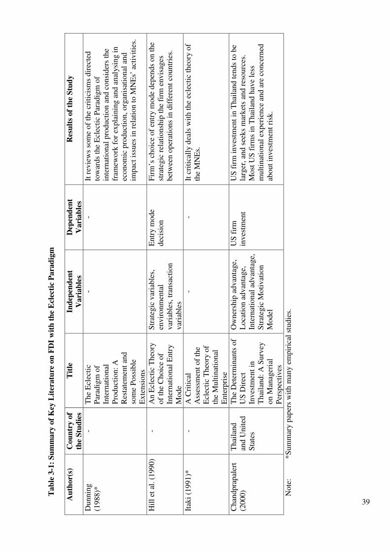
39
Tab
le 3
-1:
Su
mm
ary
of
Key
Lit
eratu
re o
n F
DI
wit
h t
he
Ecl
ecti
c P
ara
dig
m
A
uth
or(
s)
Cou
ntr
y o
f th
e S
tud
ies
Tit
le
Ind
epen
den
t V
ari
ab
les
Dep
end
ent
Vari
ab
les
Res
ult
s of
the
Stu
dy
Dunnin
g
(1988)*
-
The
Ecl
ecti
c P
arad
igm
of
Inte
rnat
ional
P
roduct
ion:
A
Res
tate
men
t an
d
som
e P
oss
ible
E
xte
nsi
ons
- -
It r
evie
ws
som
e o
f th
e cr
itic
ism
s dir
ecte
d
tow
ards
the
Ecl
ecti
c P
arad
igm
of
inte
rnat
ional
pro
duct
ion a
nd c
onsi
der
s th
e fr
amew
ork
for
expla
inin
g a
nd a
nal
ysi
ng i
n
econom
ic p
roduct
ion, org
anis
atio
nal
and
impac
t is
sues
in r
elat
ion t
o M
NE
s’ a
ctiv
itie
s.
Hil
l et
al.
(1990)
- A
n E
clec
tic
Th
eory
of
the
Choic
e of
Inte
rnat
ional
Entr
y
Mode
Str
ateg
ic v
aria
ble
s,
envir
onm
enta
l var
iable
s, t
ransa
ctio
n
var
iable
s
Entr
y m
ode
dec
isio
n
Fir
m’s
choic
e of
entr
y m
ode
dep
ends
on t
he
stra
tegic
rel
atio
nsh
ip t
he
firm
envis
ages
bet
wee
n o
per
atio
ns
in d
iffe
rent
countr
ies.
Itak
i (1
991)*
-
A C
riti
cal
Ass
essm
ent
of
the
Ecl
ecti
c T
heo
ry o
f th
e M
ult
inat
ional
E
nte
rpri
se
- -
It c
riti
call
y d
eals
wit
h t
he
ecle
ctic
theo
ry o
f th
e M
NE
s.
Chan
dpra
pal
ert
(2000)
Thai
land
and U
nit
ed
Sta
tes
The
Det
erm
inan
ts o
f U
S D
irec
t In
ves
tmen
t in
T
hai
land:
A S
urv
ey
on M
anag
eria
l P
ersp
ecti
ves
Ow
ner
ship
adv
anta
ge,
L
oca
tion a
dvan
tage,
In
tern
atio
nal
adv
anta
ge,
S
trat
egic
Moti
vat
ion
Model
US
fir
m
inves
tmen
t U
S f
irm
inves
tmen
t in
Thai
land t
ends
to b
e la
rger
, an
d s
eeks
mar
ket
s an
d r
esourc
es.
Most
US
fir
ms
in T
hai
land h
ave
less
m
ult
inat
ional
ex
per
ience
and a
re c
once
rned
ab
out
inves
tmen
t ri
sk.
Note
: *S
um
mar
y p
aper
s w
ith m
any e
mpir
ical
stu
die
s.
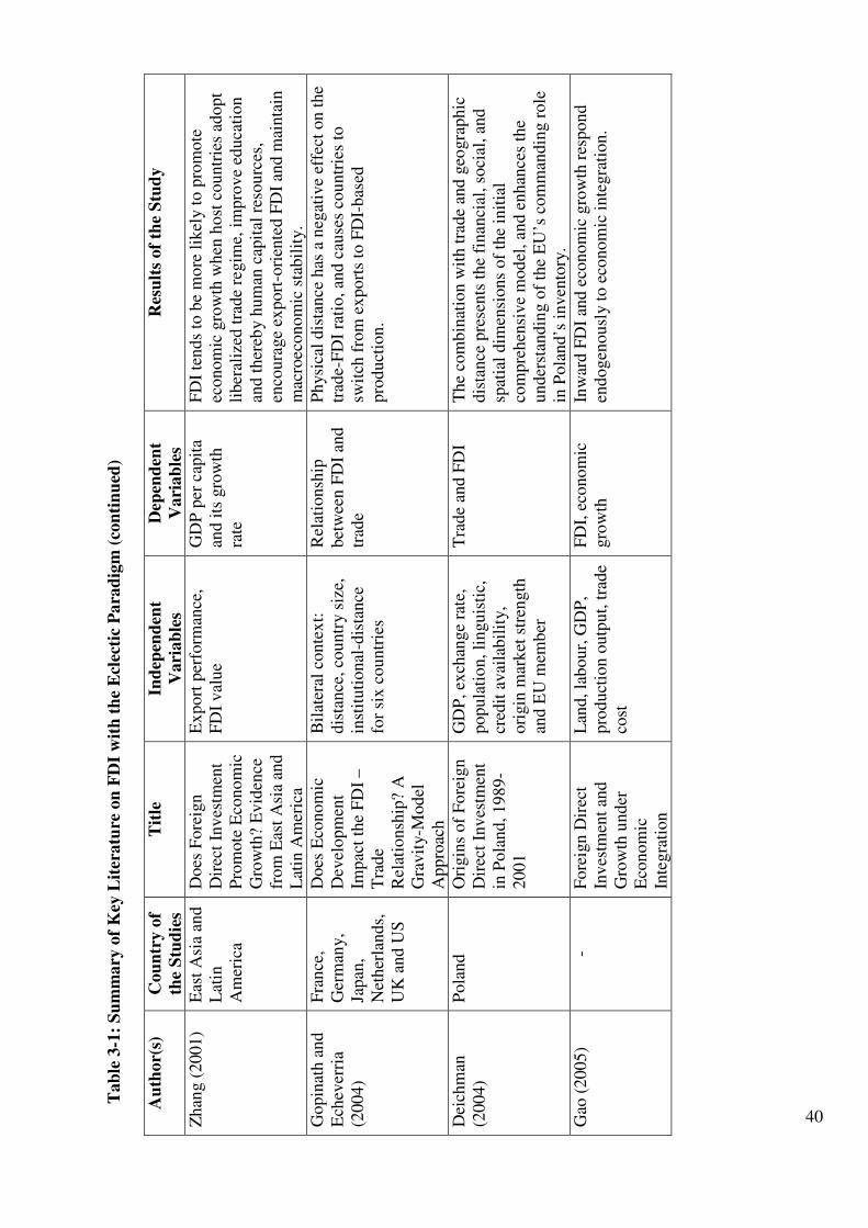
40
Tab
le 3
-1:
Su
mm
ary
of
Key
Lit
eratu
re o
n F
DI
wit
h t
he
Ecl
ecti
c P
ara
dig
m (
con
tin
ued
) Au
thor(
s)
Cou
ntr
y o
f th
e S
tud
ies
Tit
le
Ind
epen
den
t V
ari
ab
les
Dep
end
ent
Vari
ab
les
Res
ult
s of
the
Stu
dy
Zhan
g (
2001)
Eas
t A
sia
and
Lat
in
Am
eric
a
Does
Fore
ign
Dir
ect
Inv
estm
ent
Pro
mote
Eco
nom
ic
Gro
wth
? E
vid
ence
fr
om
Eas
t A
sia
and
Lat
in A
mer
ica
Ex
port
per
form
ance
, F
DI
val
ue
GD
P p
er c
apit
a an
d i
ts g
row
th
rate
FD
I te
nds
to b
e m
ore
lik
ely t
o p
rom
ote
ec
onom
ic g
row
th w
hen
host
countr
ies
adopt
liber
aliz
ed t
rade
regim
e, i
mpro
ve
educa
tion
and t
her
eby h
um
an c
apit
al r
esourc
es,
enco
ura
ge
export
-ori
ente
d F
DI
and m
ainta
in
mac
roec
onom
ic s
tabil
ity.
Gopin
ath a
nd
Ech
ever
ria
(2004)
Fra
nce
, G
erm
any,
Japan
, N
ether
lands,
U
K a
nd U
S
Does
Eco
nom
ic
Dev
elopm
ent
Impac
t th
e F
DI
–T
rade
Rel
atio
nsh
ip?
A
Gra
vit
y-M
odel
A
ppro
ach
Bil
ater
al c
onte
xt:
dis
tance
, co
untr
y s
ize,
in
stit
uti
onal
-dis
tance
fo
r si
x c
ountr
ies
Rel
atio
nsh
ip
bet
wee
n F
DI
and
trad
e
Ph
ysi
cal
dis
tance
has
a n
egat
ive
effe
ct o
n t
he
trad
e-F
DI
rati
o, an
d c
ause
s co
untr
ies
to
swit
ch f
rom
ex
port
s to
FD
I-bas
ed
pro
duct
ion.
Dei
chm
an
(2004)
Pola
nd
Ori
gin
s of
Fore
ign
Dir
ect
Inv
estm
ent
in P
ola
nd, 1989-
2001
GD
P, ex
chan
ge
rate
, popula
tion, li
nguis
tic,
cr
edit
avai
labil
ity,
ori
gin
mar
ket
str
ength
an
d E
U m
ember
Tra
de
and F
DI
The
com
bin
atio
n w
ith t
rade
and g
eogra
phic
dis
tance
pre
sents
the
finan
cial
, so
cial
, an
d
spat
ial
dim
ensi
ons
of
the
init
ial
com
pre
hen
sive
mod
el, an
d e
nhan
ces
the
under
stan
din
g o
f th
e E
U’s
com
man
din
g r
ole
in
Pola
nd’s
inven
tory
.
Gao
(2005)
- F
ore
ign D
irec
t In
ves
tmen
t an
d
Gro
wth
under
E
conom
ic
Inte
gra
tion
Lan
d, la
bour,
GD
P,
pro
duct
ion o
utp
ut,
tra
de
cost
FD
I, e
conom
ic
gro
wth
In
war
d F
DI
and e
conom
ic g
row
th r
espond
endogen
ousl
y t
o e
conom
ic i
nte
gra
tion.
41
3.3 Resource-Based Theory
The resource and capability-based advantages resulting from market segment selection and
competitive position are complementary to competitive advantages (Barney, 1991). The
Resource-Based Theory, as a strategy, is a means for achieving competitive advantage by
taking into account the positioning of the business, where to compete and how to compete
(Grant, 1991). The competitive advantage is the result of a methodical understanding of
the external and internal forces that strongly affect an organisation (Lindelöf and Löfsten,
2004). In a competitive environment, profit is likely to be associated with resource and
capability-based advantage resulting from market segment selection and competitive
position. According to the Resource-Based Theory literature, most studies confirmed that
firms possess resources that are rare, unique, and limited so as to beat their competitors in
various performance indicators. Resources are the basis of firms’ capability including
financial resource, physical resource, human resource, and organisational resource
(Barney, 1991; Grant, 1991; Idris et al., 2003; Lindelöf and Löfsten, 2004).
(1) Financial Resource
The financial resource is a requirement for firms when entering a strategic factor market
and implementing a product market strategy (Barney, 2001). The firm’s financial position
constitutes either strength or weakness and affects the firm’s ability to build distinctive
competencies in other areas (Hill and Jones, 1992). It is very important to internal firms
for driving abroad investment forward to the host country (Certo and Peter, 1991).
All firms must think carefully about financial strategies, including different sources of
capital, the capital structure, the cost of capital of the enterprises, and the effect of dividend
policy (Ansoff, 1984; Bowman and Asch, 1987). Brown and Gutterman (2003) identified
the key financial factors as: (1) historical financial statements, which indicate the firm’s
current position and how the firm has been managed in the past; (2) pro forma financial
statements, which state the risk of the business and performance; and (3) operating
budgets, which impact the firm’s operation.
The financial performance is very important for companies’ stakeholders because they
need assurance that companies can survive. One feature of the financial performance is the
42
financial ratio to assets which indicates the financial strengths and weaknesses of firms. A
widely used term in financial analysis is the return on investment (ROI). ROI is a return
on total assets, return on common equity or on book value, and gross profit margin
(Cooley, 1994).
The successes of firms include not only improving the financial statement but also the
marketing strategy to measure the firms’ performance. Finance and marketing must work
together to devise complete products and services and drive them to commanding positions
in a defensible market segment (Davidow, 1986; Idris et al., 2003; Marr et al., 2004).
(2) Physical Resource
Penrose (1959) originally split the firm’s resources into physical and human, and defined
the physical resource as tangible things such as plant, equipment, land, and natural
resources. Williamson (1975) emphasized the importance of physical resource to gain a
competitive advantage. Chatterjee and Wernerfelt (1991) stated that the physical resource
of a firm is characterized by fixed capacity. The physical resource is able to assess the
capacity available for diversified expansion of the stock beyond the requirements of the
current investment firms.
Marr et al. (2004) included all tangible infrastructure assets, such as structural layout and
information and communication technology, which contains databases, servers, and
physical networks like intranets into the physical resource.
(3) Human Resource
Penrose (1959), in his split of the firm’s resources into physical and human, identified
human resource as a key asset of the firm. Becker (1976) used the phrase human resource
to define a core asset of an organisation. Hall (1992) underlined skills and know-how as
important and Roos (1998) defined the human resource as knowledge, skills, and
experience of employees. Human resource, therefore, includes employees’ skills,
competences, commitment, motivation, and loyalty. Others (Barney, 2001; Harvey and
Bowin, 1996; McGoldrick et al., 2002) added the technical expertise and problem-solving
capability, creativity, education, and attitude into the definition of human resource.

43
Human resources include training, education, judgement, intelligence, relationships, and
insight of individuals and workers in firms, and these are central to sustaining competitive
advantages. Previous studies on human resource and firm performance agreed that this
resource is able to improve the firms’ efficiency and effectiveness (Barney, 1991;
Elmawazini et al., 2005; Grant, 1991) and has a direct impact on the firms’ potential
performance and moderate relationships between strategy and performance. Furthermore,
in order to achieve the firms’ objectives of maximising profits, high control level, and low
cost transactions, firms need to increase employee participation in the work process and
adopt work-force planning (Hill and Jones, 1992).
(4) Organisational Resource
Previous researchers (Chaterjee and Wernerfelt, 1991; Hall, 1992; Idris et al., 2003) stated
that the organisational resource refers to the intangible resource that is very critical for
firms in making decisions and policies. Today’s competitive advantages come from better
utilisation of the intangible resource such as technology, patents, trade marks, copyrights,
registered designs, trade secrets and processes, technical employees, and research facilities.
Chatterjee and Wernerfelt (1991) also included brand name and reputation in the
organisational resource.
Bettis (1981) suggested that firms achieved better performance because they were open to
the possibility of differentiation and segmentation which are associated with accounting
determined risk, R&D expenditures, and capital intensity. Furthermore, the finding
showed that R&D is the most important determinant in the performance advantage.
Chatterjee and Wernerfelt (1991), Grindley and Teece (1997), and Hall (1992) supported
Bettis’s suggestion on how the organisational resource is being handled and how work
flows through the organisation with modest cost in the effectiveness of original operations.
The Resource-Based Theory has been developed to explain how organisations achieve
sustainable competitive advantage (Calderia and Ward, 2003). Accordingly, firms must
look for unique attributes that may provide superior performance (Barney, 1991; Caldeira
and Ward, 2003).
44
3.3.1 Applications of Resource-Based Theory
Rugman (1988) studied the structure and performance of 16 resource-based Canadian
MNEs that engaged in FDI. It was apparent that substantial environmental limitations
determined FDI as a foreign entry mode. These Canadian MNEs demonstrated the success
of managerial strategies aimed at marketing rather than production. They built on the
resource strength and process and distributed products aggressively on a worldwide basis.
Closs and Thompson (1992) added infrastructure management (facilities design, location
analysis, channel analysis, inventory planning, and information system) into their study as
part of the physical resource. The authors suggested the infrastructure manager focus on
integrating business functions rather than on market or product segment, and on variances
from targets rather than on absolute cost levels.
Loungani and Razin (2001) suggested in their study that FDI contributes to investment and
growth in host countries through various channels such as technology transformation,
human capital development by employee training programmes, and corporate tax revenues.
The authors suggested that developing countries should focus on improving the investment
climate in all kinds of capital, both domestic and foreign, to attract FDI.
Schroeder et al. (2002) examined the manufacturing strategy from the perspective of the
resource-based view (RBV) based on Barney (1991) and Grant’s (1991) findings and
Rugman (1988) study of the firm, by examining how 164 manufacturing plants (in
Germany, Italy, Japan, UK, and the US) developed capabilities and resources in pursuit of
better performance and competitive advantage. The RBV implies that such innovations
can contribute to competitive advantage and cannot be easily duplicated.
Chen and Ku (2002) highlighted the FDI as a strategic move by foreign investors to exploit
host country resources. These are not equally available to all firms and hence created a
competitive advantage for those firms. The authors, using Taiwanese firms as an example,
found the resource-based FDI strategy to be most effective among large firms in mature
industries. A similar study in the international competitiveness of Korean enterprises by
Ray et al. (2004) showed that Korea has successfully made the transition from resource-
based industries to high technology industries.
45
In summary, the Resource-Based Theory can be used to explain success in FDI in
Thailand. This theory explains how internal contextual factors of a firm (such as human
and financial resources, intangible resources) can adapt to the external economic
environment (such as inflation rate and wage rate from investing partners). Therefore, the
Resource-Based Theory is used to analyse and understand why and how the attributes of
these factors caused different levels of FDI success across countries. The Resource-Based
Theory can also explain the knowledge and performance indicators in most models (Idris
et al., 2003). Table 3-2 shows a summary of key literature on FDI with the Resource-
Based Theory.
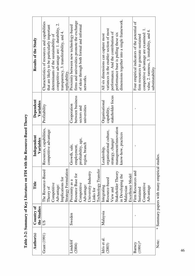
46
Tab
le 3
-2:
Su
mm
ary
of
Key
Lit
eratu
re o
n F
DI
wit
h t
he
Res
ou
rce-
Base
d T
heo
ry
Au
thor(
s)
Cou
ntr
y o
f th
e S
tud
ies
Tit
le
Ind
epen
den
t V
ari
ab
les
Dep
end
ent
Vari
ab
les
Res
ult
s of
the
Stu
dy
Gra
nt
(1991)
US
T
he
Res
ourc
e-B
ased
T
heo
ry o
f C
om
pet
itiv
e A
dvan
tage:
Im
pli
cati
ons
for
Str
ateg
y F
orm
ula
tion
Res
ourc
es, ca
pab
ilit
ies,
co
mpet
itiv
e ad
van
tage
P
rofi
tabil
ity
Char
acte
rist
ics
of
reso
urc
es a
nd c
apab
ilit
ies
that
are
lik
ely t
o b
e par
ticu
larl
y i
mport
ant
det
erm
inan
ts o
f th
e su
stai
nab
ilit
y o
f co
mpet
itiv
e ad
van
tage
are:
1. dura
bil
ity, 2.
tran
spar
ency
, 3. tr
ansf
erab
ilit
y, a
nd 4
. re
pli
cabil
ity.
Lin
del
öf
(2004)
Sw
eden
P
rox
imit
y as
a
Res
ourc
e B
ase
for
Com
pet
itiv
e A
dvan
tage:
U
niv
ersi
ty-I
ndust
ry
Lin
ks
for
Tec
hnolo
gy T
ransf
er
Gro
wth
, sa
le,
emplo
ym
ent,
pro
fita
bil
ity, ag
e,
regio
n, bra
nch
Cooper
atio
n
bet
wee
n b
usi
nes
s se
ctors
and
univ
ersi
ties
Pro
xim
ity
bet
wee
n n
ew t
echnolo
gy-b
ased
fi
rms
and u
niv
ersi
ties
pro
mote
the
exch
ange
of
idea
s th
rou
gh b
oth
form
al a
nd i
nfo
rmal
net
work
s.
Idri
s et
al.
(2
003)
Mal
aysi
a In
tegra
tin
g
Res
ourc
e-b
ased
V
iew
and
Sta
keh
old
er T
heo
ry
in D
evel
opin
g t
he
Mal
aysi
an
Ex
cell
ence
Model
Lea
der
ship
, org
anis
atio
nal
cult
ure
, st
rate
gy, ch
ange/
m
anag
emen
t/in
novat
ion
know
-how
, pra
ctic
es
Org
anis
atio
nal
ca
pab
ilit
y,
stak
ehold
er f
ocu
s
All
six
dim
ensi
ons
can c
aptu
re m
ost
var
iance
s in
the
enab
ler
sect
ion o
f m
ost
per
form
ance
. A
nd
the
contr
ibuti
on o
f per
form
ance
bas
e is
pull
ing t
hes
e si
x
dim
ensi
ons
toget
her
into
a s
ingle
fra
mew
ork
.
Bar
ney
(1
991)*
-
Fir
m R
esourc
es a
nd
Sust
ained
C
om
pet
itiv
e A
dvan
tage
- -
Four
empir
ical
indic
ators
of
the
pote
nti
al o
f fi
rm r
esourc
es t
o g
ener
ate
sust
ained
co
mpet
itiv
e ad
van
tage
are
exam
ined
: 1.
val
ue,
2. ra
renes
s, 3
. im
itab
ilit
y, an
d 4
. su
bst
ituta
bil
ity
Note
:
* S
um
mar
y p
aper
s w
ith m
any e
mpir
ical
stu
die
s.
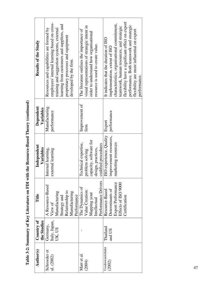
47
Tab
le 3
-2:
Su
mm
ary
of
Key
Lit
eratu
re o
n F
DI
wit
h t
he
Res
ou
rce-
Base
d T
heo
ry (
con
tin
ued
) Au
thor(
s)
Cou
ntr
y o
f th
e S
tud
ies
Tit
le
Ind
epen
den
t V
ari
ab
les
Dep
end
ent
Vari
ab
les
Res
ult
s of
the
Stu
dy
Sch
roed
er e
t al
. (2
002)
Ger
man
y,
Ital
y, Ja
pan
, U
K, U
S
A R
esourc
e-B
ased
V
iew
of
Man
ufa
cturi
ng
Str
ateg
y a
nd
Rel
atio
nsh
ip t
o
Man
ufa
cturi
ng
Per
form
ance
Inte
rnal
lea
rnin
g,
exte
rnal
lea
rnin
g
Man
ufa
cturi
ng
per
form
ance
R
esourc
es a
nd c
apab
ilit
ies
are
form
ed b
y
emplo
yee
s' i
nte
rnal
lea
rnin
g b
ased
on c
ross
-tr
ainin
g a
nd s
ugges
tion s
yst
ems,
ex
tern
al
lear
nin
g f
rom
cust
om
ers
and s
uppli
ers,
and
pro
pri
etar
y p
roce
sses
and
equip
men
t dev
eloped
by t
he
firm
.
Mar
r et
al.
(2
004)
- T
he
Dynam
ics
of
Val
ue
Cre
atio
n:
Map
pin
g y
our
Inte
llec
tual
P
erfo
rman
ce D
riv
ers
Tec
hnic
al e
xper
tise
, pro
ble
m s
olv
ing
capac
ity, so
ftw
are
for
des
ign, pra
ctic
es,
codif
ied p
roce
dure
s
Impro
vem
ent
of
firm
T
he
lite
ratu
re o
utl
ines
th
e im
port
ance
of
vis
ual
rep
rese
nta
tions
of
stra
tegic
inte
nt
in
ord
er t
o u
nder
stan
d h
ow
org
anis
atio
nal
re
sourc
e is
use
d t
o c
reat
e val
ue.
Uss
ahaw
anit
chak
it
(2002)
Thai
land
and U
S
Res
ourc
e-B
ased
D
eter
min
ants
of
Ex
port
Per
form
ance
E
ffec
ts o
f IS
O 9
000
Cer
tifi
cati
on
ISO
ex
per
ience
, Q
ual
ity
impro
vem
ent
reso
urc
es,
mar
ket
ing r
esourc
es
Ex
port
per
form
ance
It
indic
ates
that
the
dura
tion o
f IS
O
imple
men
tati
on, ex
tent
of
ISO
ch
arac
teri
stic
s, o
rgan
isat
ional
com
mit
men
t,
team
work
, hum
an r
esourc
es, an
d s
trat
egic
fl
exib
ilit
y h
ave
a si
gnif
ican
t ef
fect
on e
xport
per
form
ance
. B
oth
tea
mw
ork
and s
trat
egic
fl
exib
ilit
y ar
e m
ore
infl
uen
tial
on e
xport
per
form
ance
.
48
3.4 Business Network Theory
The Business Network Theory is a set of relationships between firms, including strategic
alliances, joint ventures, long-term buyer-supplier partnerships, and collaborative
relationships (Chen and Chang, 2004; Ebers and Jarillo, 1998; Gowa and Mansfield, 2004;
Jarillo, 1988). The network theory was started by sociologists who used networks to
understand norms, exchanges, and power during the 1960s and the 1970s. Since the 1980s,
the ‘network’ concept has been more fashionable in social science applied to business.
Gulati (1999) referred to the networks by following the ‘invisible hand’ of Alfred Chandler
(1977) as a concept akin to the notion of social capital that has been developed for
understanding individual networks. Castells (2000) considered the network as a new form
of paradigm and regarded the network as the fundamental node from which new
organisations are and will be made. Mills et al. (2003) stated that networks are the interest
groups within the company and involve company personnel with suppliers, customers,
legislative authorities, or advisers. They also include reputation and brand as part of
network.
A network can be defined as: “a long-term relationship between organizations as actors
that share resources to achieve negotiated actions for joint objectives” (Porras et al., 2004,
p. 354). Similarly, Backman and Butler (2003) defined the network as a long-term
purposeful arrangement among distinct but related for-profit organisations that allows
those firms to gain or sustain a competitive advantage vis-a-vis their competitors outside
the network. DeBresson and Amesse (1991) developed the network theory into two
different levels: (1) international strategic alliances; and (2) regional networks, where the
regional networks are the main loci of technological and economic externalities that benefit
FDI.
Business networks with high embeddedness can develop trust (Ebers and Jarillo, 1998;
Jarillo, 1988; Newell and Swan, 2000) and support a rich exchange of information among
their members. Business networks are information repositories. Members of business
networks develop appropriate organisational structures and inter-organisational interaction
routines, improving technology and operation activities. Facing radical innovation
49
opportunities that arise, business networks need to regroup their members to access new
knowledge. Accordingly, a high degree of embeddedness of business networks is related
to the capacity for incremental innovation, whereas a low degree of embeddedness is
related to the capacity for radical innovation (Chen and Chang, 2004).
The purpose of networks through FDI is to tap into the resources in a foreign market and to
serve as a source of sustainable competitive advantage, such as market intelligence,
technological know-how, management expertise, or simply reputation for being established
in a prestigious market (Chen and Chen, 1998; Gulati et al., 2000). This theory enables
investors to gain economies of scale and scope, to improve the efficiency of operations, to
reduce the vulnerability to market fluctuations, and to pave the way for further growth in
the future.
Networks can be created and sustained by the basic condition for efficiency that is the gain
accrued by being part of the network over the long term. This can be achieved through the
realisation of two points: (1) belonging to the network gives superior performance (thus
there is more pie to share, because the network is effective); and (2) the sharing
mechanisms are ‘fair’. Efficiency and effectiveness are the basic conditions of existence of
networks applying through the firms.
3.4.1 Applications of Business Network Theory
Jarillo (1988) employed a simple transaction cost model to determine whether firms should
produce internally or outsource. The research findings showed the total cost of
outsourcing partners is lower than the internal production cost, and firms should not
internalize the production activities but outsource them through collaboration with
partners. Chen and Chang (2004) supported Jarillo’s findings that business networks
develop social capital and routines to create value and reduce transaction costs. They are
very beneficial to firms but cannot reduce competition.
Chen et al. (2004) used Taiwanese manufacturing firms investing abroad to analyse the
pattern of local linkages as an investment local relationship. The authors defined a
network as a set of interconnected business relationships upon which exchanges between
activities are conducted as: (1) sourcing of components and parts; (2) marketing of final
products; (3) product design and innovation; (4) hiring of local labour; (5) sourcing of local
50
production capacities; and (6) obtaining financial resources. The findings showed the local
linkage intensity of a foreign subsidiary differed by FDI location, entry mode, firm size,
and the nature of the production network in which an investor is embedded. More local
linkages will be pursued by an investor if it is in search of distinctive and unique
reproducible resources (workers, components and parts, subcontracting, and source of
R&D).
Girod and Rugman (2005) examined the retail multinational enterprise relationship
between FDI and business networks. The authors tried to explain the internalisation of
three retailers (UK-based multinational retailers – Tesco, the Body Shop, and French-based
global retailer – Moet Hennessy Louis Vuitton) whose geographic scope, sectoral
conditions and competitive strategies differed substantially. Their findings supported those
of Chen et al. (2004) as evidence of strong network relationships can succeed in
overcoming internal and/or environmental constraints to cross-border resources transfer.
However, the authors found that the business relationship can be more successful in
countries where there are barriers to FDI.
The Business Network Theory explains how business firms and organisations in Thailand
can form alliances, economic integrations and trade agreements to improve production and
reduction production costs. For example, Thailand’s natural resources, abundant labour,
and growing markets in the region present great investment opportunity for foreign
investors to form alliances. In addition, Thailand is a member of several economic
integrations such as APEC and ASEM and this is an added advantage in drawing inflows
of FDI into Thailand.
Table 3-3 presents a summary of key literature on FDI with the Business Network Theory.
There are many studies which explore the relationships between FDI firms and Business
Network Theory. The results from most of these studies suggest that firms can increase
their performances with the cost reduction related to the Business Network Theory (see
Table 3-3).
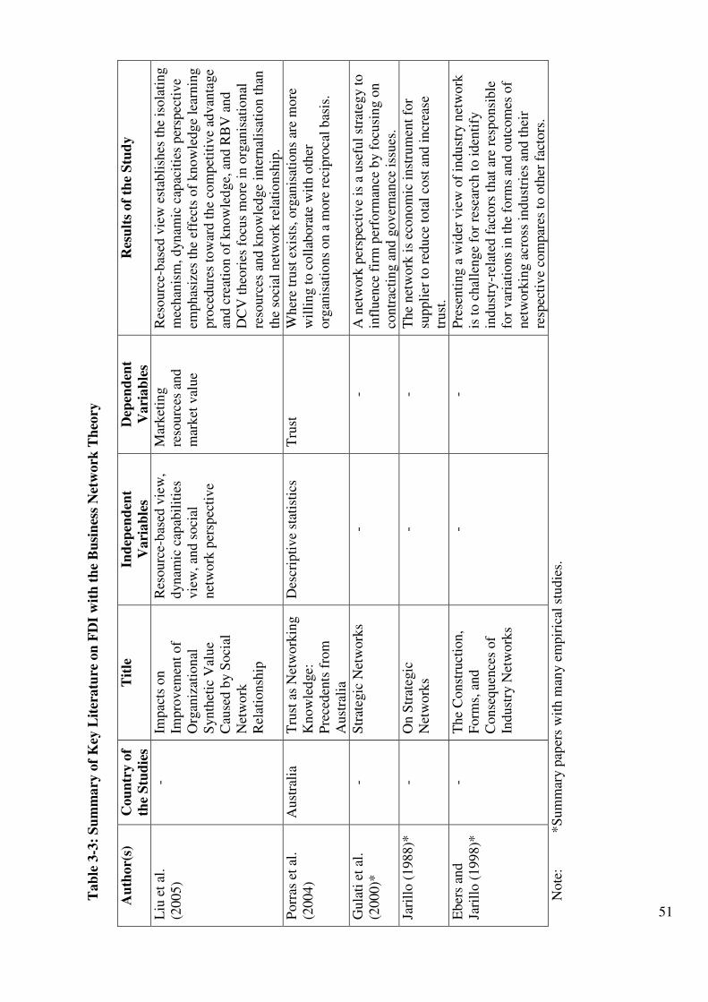
51
Tab
le 3
-3:
Su
mm
ary
of
Key
Lit
eratu
re o
n F
DI
wit
h t
he
Bu
sin
ess
Net
work
Th
eory
Au
thor(
s)
Cou
ntr
y o
f th
e S
tud
ies
Tit
le
Ind
epen
den
t V
ari
ab
les
Dep
end
ent
Vari
ab
les
Res
ult
s of
the
Stu
dy
Liu
et
al.
(2005)
- Im
pac
ts o
n
Impro
vem
ent
of
Org
aniz
atio
nal
S
ynth
etic
Val
ue
Cau
sed b
y S
oci
al
Net
work
R
elat
ionsh
ip
Res
ourc
e-b
ased
vie
w,
dynam
ic c
apab
ilit
ies
vie
w, an
d s
oci
al
net
work
per
spec
tive
Mar
ket
ing
reso
urc
es a
nd
mar
ket
val
ue
Res
ourc
e-b
ased
vie
w e
stab
lish
es t
he
isola
ting
mec
han
ism
, d
yn
amic
cap
acit
ies
per
spec
tive
emphas
izes
the
effe
cts
of
know
ledge
lear
nin
g
pro
cedure
s to
war
d t
he
com
pet
itiv
e ad
van
tage
and c
reat
ion o
f know
led
ge,
and R
BV
and
DC
V t
heo
ries
focu
s m
ore
in o
rgan
isat
ional
re
sourc
es a
nd k
now
led
ge
inte
rnal
isat
ion t
han
th
e so
cial
net
work
rel
atio
nsh
ip.
Porr
as e
t al
. (2
004)
Aust
rali
a T
rust
as
Net
work
ing
Know
led
ge:
P
rece
den
ts f
rom
A
ust
rali
a
Des
crip
tive
stat
isti
cs
Tru
st
Wher
e tr
ust
ex
ists
, org
anis
atio
ns
are
more
w
illi
ng t
o c
oll
abora
te w
ith o
ther
org
anis
atio
ns
on a
more
rec
ipro
cal
bas
is.
Gula
ti e
t al
. (2
000)*
-
Str
ateg
ic N
etw
ork
s -
- A
net
work
per
spec
tive
is a
use
ful
stra
teg
y t
o
infl
uen
ce f
irm
per
form
ance
by f
ocu
sin
g o
n
contr
acti
ng a
nd g
ov
ernan
ce i
ssues
.
Jari
llo (
1988)*
-
On S
trat
egic
N
etw
ork
s -
- T
he
net
work
is
econom
ic i
nst
rum
ent
for
suppli
er t
o r
educe
tota
l co
st a
nd i
ncr
ease
tr
ust
.
Eber
s an
d
Jari
llo (
1998)*
-
The
Const
ruct
ion,
Form
s, a
nd
Conse
quen
ces
of
Indust
ry N
etw
ork
s
- -
Pre
senti
ng a
wid
er v
iew
of
indust
ry n
etw
ork
is
to c
hal
lenge
for
rese
arch
to i
den
tify
in
dust
ry-r
elat
ed f
acto
rs t
hat
are
res
ponsi
ble
fo
r var
iati
ons
in t
he
form
s an
d o
utc
om
es o
f net
work
ing a
cross
indust
ries
and t
hei
r re
spec
tive
com
par
es t
o o
ther
fac
tors
.
Note
: *S
um
mar
y p
aper
s w
ith m
any e
mpir
ical
stu
die
s.

52
Tab
le 3
-3:
Su
mm
ary
of
Key
Lit
eratu
re o
n F
DI
wit
h t
he
Bu
sin
ess
Net
work
Th
eory
(co
nti
nu
ed)
Au
thor(
s)
Cou
ntr
y o
f th
e S
tud
ies
Tit
le
Ind
epen
den
t V
ari
ab
les
Dep
end
ent
Vari
ab
les
Res
ult
s of
the
Stu
dy
Chen
and C
hen
(1
998)
US
, C
hin
a,
and
South
east
A
sia
Net
work
Lin
kag
es
and L
oca
tion C
hoic
e in
Fore
ign D
irec
t In
ves
tmen
t
Net
work
lin
kag
es,
firm
-sp
ecif
ic a
sset
s, a
nd
loca
tion-s
pec
ific
fac
tors
Net
work
lin
kag
es
Tai
wan
ese
firm
s ar
e kee
n o
n m
akin
g e
xte
rnal
li
nkag
es, but
are
indif
fere
nt
to, or
inca
pab
le
of,
mak
ing i
nte
rnal
lin
kag
es t
hro
ugh F
DI.
New
ell
and
Sw
an (
2000)
UK
T
rust
and I
nte
r-O
rgan
izat
ional
N
etw
ork
ing
Des
crip
tion
Tru
st
Inte
r-org
anis
atio
nal
and m
ult
i-fu
nct
ional
net
work
ing i
s in
crea
sin
g w
ithin
univ
ersi
ties
as
wel
l as
busi
nes
s org
anis
atio
ns.
DeB
ress
on a
nd
Am
esse
(1
991)*
- N
etw
ork
s of
Innov
ators
: A
R
evie
w a
nd
Intr
odu
ctio
n t
o t
he
Issu
e
- -
The
net
work
appro
ach a
llow
s th
e in
corp
ora
tion o
f m
any c
om
ple
men
tary
and
rece
ntl
y d
evel
oped
str
ands
of
anal
ysi
s an
d
aspec
ts o
f in
novat
ion.
Chen
and
Chan
g (
2004
)*
- D
yn
amic
s of
Busi
nes
s N
etw
ork
E
mbed
ded
nes
s
- -
Fir
ms
stri
ve
to i
ncr
ease
res
ourc
e v
alue
and
reduce
tra
nsa
ctio
n c
ost
s th
rough i
nte
r-fi
rm
spec
iali
sati
on, re
lati
onal
cap
ital
and r
outi
nes
, an
d l
etti
ng b
usi
nes
s net
work
s bec
om
e gra
dual
ly e
mbed
ded
in a
n e
volu
tionar
y
pro
cess
.
Gow
a an
d
Man
sfie
ld
(2004)
Fra
nce
, G
erm
any,
UK
, It
aly,
Russ
ia, U
S,
Japan
All
iance
s, I
mper
fect
M
arket
s, a
nd M
ajo
r-P
ow
er T
rad
e
GN
P, D
ista
nce
, D
emocr
acy, A
lly,
Reg
ion g
roupin
g
Ex
port
A
llia
nce
s ca
n s
uppo
rt a
n o
pti
mal
lev
el o
f tr
ade
and e
xer
t a
stro
nger
infl
uen
ce o
n t
rade
in g
oods
pro
duce
d u
nder
condit
ions
of
incr
easi
ng r
ather
than
co
nst
ant
retu
rns
to
scal
e.
Note
: * S
um
mar
y p
aper
s w
ith a
ny e
mpir
ical
stu
die
s.

53
3.5 Summary
This chapter briefly reviews three important FDI theories such as the Eclectic Paradigm,
the Resource-Based Theory and Business Network Theory. The chapter begins with an
overview of the FDI followed by a critique of the role of government, its impact on
investment policy, and a review of the literature on general theories of FDI. The
determinants of FDI and its impact to the host country are also discussed. FDI can be
regarded as a firm’s strategy in achieving its goal to gain more profit and/or serve the
foreign markets. However, FDI inflows affect the host economy in several ways, with
both positive and negative impacts to the host and home economy.
In the early stage of FDI, Dunning’s Eclectic Paradigm was useful in explaining FDI
characteristics and the firms’ specific advantages. Basically, this theory suggests that the
tendency of a firm to engage in foreign production depends on its OLI configuration in the
target market. Even though there are many different modes to enter foreign production for
a firm, FDI is the main mode to capture a foreign market if the firm has the capacity to
utilize all OLI advantages. Dunning (1980) denoted that the firm's FDI decision is
influenced by three factors: ownership, location, and internalisation. The paradigm
explains how FDI affects the distribution of ownership advantages between the firms of
different origins and the configuration of ownership, location, and internalisation specific
advantages. Many researchers use the Eclectic Paradigm concept to determine and explain
the dynamic effects of firms in terms of marketing and investment in various countries.
The Resource-Based Theory focuses on resources rather than products (Kim, 2000).
According to the theory, a firm’s capability to handle its competitiveness depends on its
competence in firm-specific resources and its unique potential in terms of technical know-
how and professional ability. Most social science, investment, and marketing research use
this theory to understand the external and internal forces to organisations’ diversification
strategy.
The Business Network Theory is a field of social science applied to business. It is a set of
relationships between firms to support the exchange of information among members. The
network develops suitable organisational structures and inter-organisational interaction
routines, improving technology and operation activities.
CHAPTER 4
GRAVITY MODEL AND FDI
The theoretical foundation and empirical relevance of FDI have been discussed in Chapter
3. The FDI discussion was based on the conceptual framework of the Eclectic Paradigm
introduced by Dunning (1980). The concept of the Eclectic Paradigm can be applied to the
locational variables in the empirical models in this study to identify potential factors in
influencing foreign investment decision. Characteristics such as market size, market
growth, economic development, agglomeration, labour costs, governmental and integration
policies discussed in the Eclectic Paradigm are used to analyse FDI determinants.
The Resource-Based Theory provides possible internal factors in home and host countries.
This theory complements the empirical models in explaining FDI decisions and trends a
country should pursue. The theory suggests how Thailand can improve the investment
climate to attract more FDI and sustain its economy.
Finally, the Business Network Theory is used to explain the collaborative relationships
between the 21 investing partners and Thailand. The theory explains why regional
integrations, such as APEC and ASEM, are included in the empirical models. The theory
explains and evaluates the benefits of being a member of the regional integrations.
However, the literature on the incentives for FDI is enormous. Since FDI is considered as
a form of international capital movement, a number of theories have been developed to
explain FDI trends. At this point, it is possible to answer the questions: ‘why do firms
locate their operation overseas?’ and ‘what advantages do home and host countries have?’.
Chapter 3 reviews the literature in the areas of FDI and provides some key concepts from
the relevant literature in order to frame the determinants of FDI and the main hypotheses
analysed in Chapter 5.
The empirical models use some of the concepts from the three theories to explain and
discuss foreign investment flows into Thailand. This includes investigating the reasons
why foreign investors favour close-by countries with similar characteristics and familiar
environments over the gravity factor and institutionally different countries (Guerin, 2006).
55
Besides physical distance, the extended Gravity Model identifies the flows of FDI from the
21 investing partners to Thailand, which can be explained by supply side of investing
partners, demand conditions of Thailand, and other economic factors (such as regional
integration) which can either assist or resist the movements of investment flows.
Recently, the Gravity Model (Buch et al., 2003) has become a popular method to analyse
the importance of countries’ attractive location factors for FDI. The Gravity Model has
performed remarkably well as an empirical framework for explaining investment flows
(Martinez-Zarzoro and Nowak-Lehmann, 2004) and identifying the common determinants
of FDI across countries (Bevan and Estrin, 2004; Brenton et al., 1999; Wei and Wu, 2001).
The Gravity Model is based on the interactions of various potential sources across border.
The model has an inverse relationship between origins and destinations. The model is also
designed to account for the behaviour of large groups of people, commodities, trade, and
investment that is appropriate to investigate the determinants of the inflows of FDI and FPI
into Thailand. On the other hand, the distance from various origins to destinations is not
considered in other FDI studies. Therefore, the Gravity Model is a static formulation
which is capable of explaining factors that attract inflows of foreign investment into
Thailand.
The first part of this chapter provides a background to the Gravity Model. The theoretical
framework of the Gravity Model in both trade and FDI is discussed in Sections 4.2 and 4.3,
respectively. The last section summarises the chapter.
4.1 Background to the Gravity Model
The Gravity Model is based on an analogy of Newton’s Law of Gravitation and is used to
predict the movement of information and commodities between different places related to
the distance between them (Erlander, 1980; Rosenberg, 2004). According to Cheng and
Wall (as cited in Cortes-Rodriguez, 2002), the variants of the gravity equation have been
used in the social sciences since the 1860s, when Carey applied Newtonian physics to
study human behaviour. The Gravity Model has become popular and has often been used
in the field of social science since William J. Reilly set up the Reilly’s Law of Retail
Gravitation in 1931.
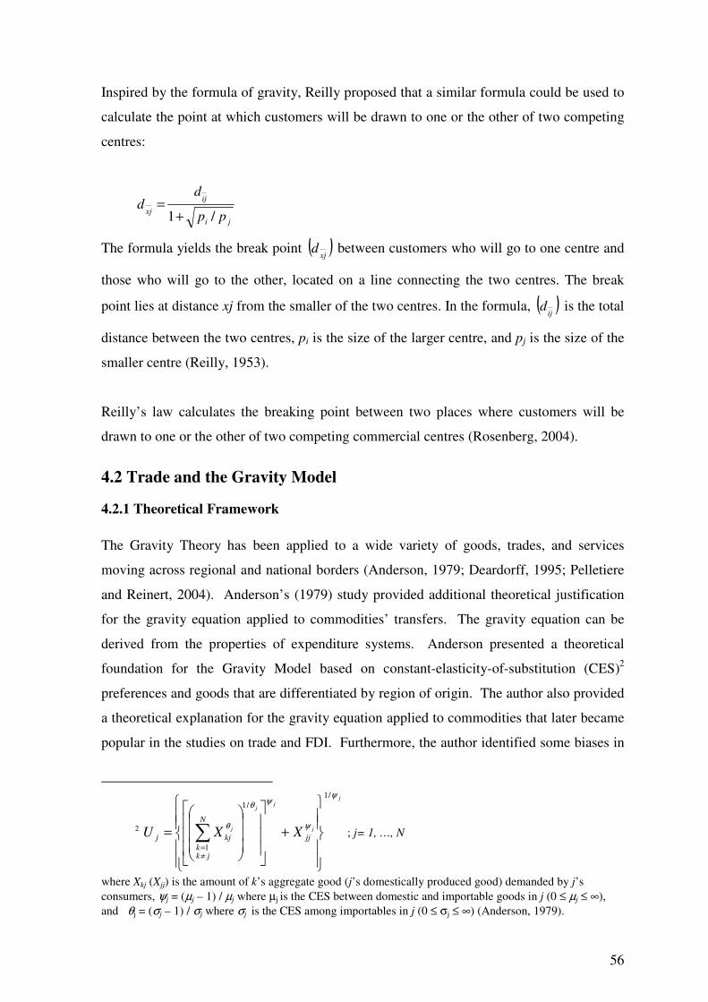
56
Inspired by the formula of gravity, Reilly proposed that a similar formula could be used to
calculate the point at which customers will be drawn to one or the other of two competing
centres:
ji
ij
xjpp
dd
/1+=
The formula yields the break point ( )xj
d between customers who will go to one centre and
those who will go to the other, located on a line connecting the two centres. The break
point lies at distance xj from the smaller of the two centres. In the formula, ( )ij
d is the total
distance between the two centres, pi is the size of the larger centre, and pj is the size of the
smaller centre (Reilly, 1953).
Reilly’s law calculates the breaking point between two places where customers will be
drawn to one or the other of two competing commercial centres (Rosenberg, 2004).
4.2 Trade and the Gravity Model
4.2.1 Theoretical Framework
The Gravity Theory has been applied to a wide variety of goods, trades, and services
moving across regional and national borders (Anderson, 1979; Deardorff, 1995; Pelletiere
and Reinert, 2004). Anderson’s (1979) study provided additional theoretical justification
for the gravity equation applied to commodities’ transfers. The gravity equation can be
derived from the properties of expenditure systems. Anderson presented a theoretical
foundation for the Gravity Model based on constant-elasticity-of-substitution (CES)2
preferences and goods that are differentiated by region of origin. The author also provided
a theoretical explanation for the gravity equation applied to commodities that later became
popular in the studies on trade and FDI. Furthermore, the author identified some biases in
2
j
j
jj
j
jj
N
jkk
kjj XXU
ψ
ψ
ψθ
θ
/1
/1
1
+
= ∑≠=
; j= 1, …, N
where Xkj (Xjj) is the amount of k’s aggregate good (j’s domestically produced good) demanded by j’s
consumers, ψj = (µj – 1) / µj where µj is the CES between domestic and importable goods in j (0 ≤ µj ≤ ∞),
and θj = (σj – 1) / σj where σj is the CES among importables in j (0 ≤ σj ≤ ∞) (Anderson, 1979).
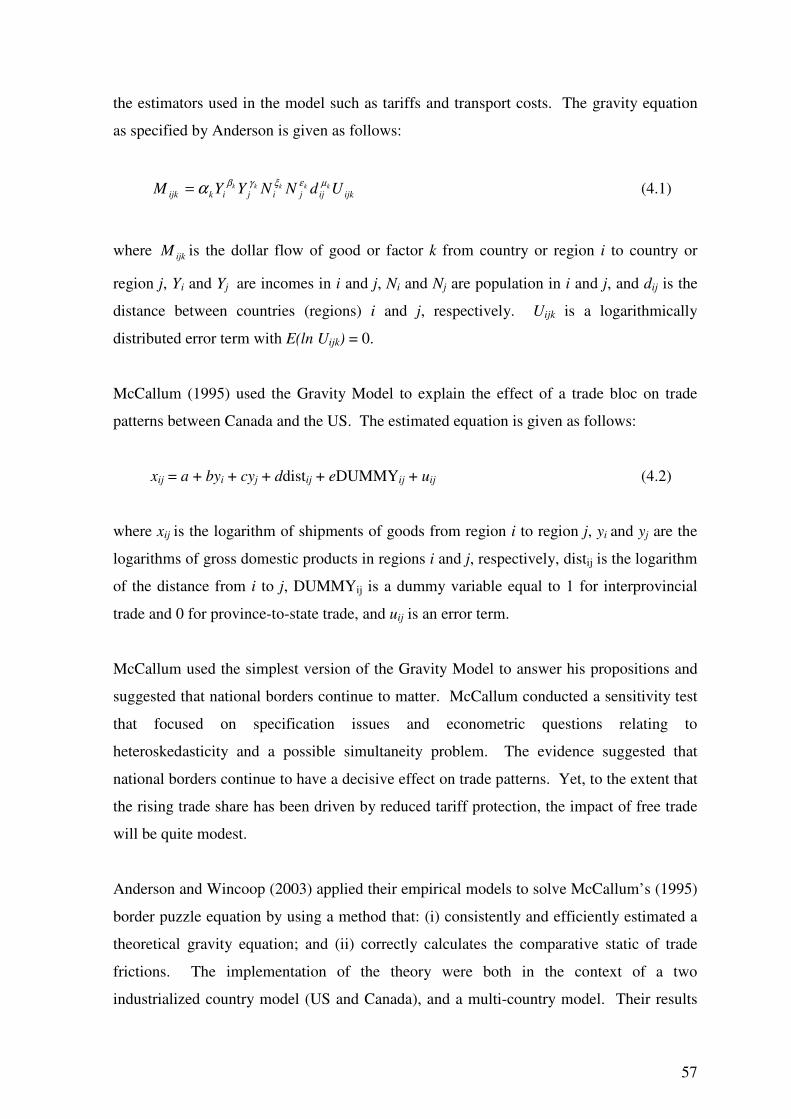
57
the estimators used in the model such as tariffs and transport costs. The gravity equation
as specified by Anderson is given as follows:
ijkijjijikijk UdNNYYM kkkkk µεξγβα= (4.1)
where ijkM is the dollar flow of good or factor k from country or region i to country or
region j, Yi and Yj are incomes in i and j, Ni and Nj are population in i and j, and dij is the
distance between countries (regions) i and j, respectively. Uijk is a logarithmically
distributed error term with E(ln Uijk) = 0.
McCallum (1995) used the Gravity Model to explain the effect of a trade bloc on trade
patterns between Canada and the US. The estimated equation is given as follows:
xij = a + byi + cyj + ddistij + eDUMMYij + uij (4.2)
where xij is the logarithm of shipments of goods from region i to region j, yi and yj are the
logarithms of gross domestic products in regions i and j, respectively, distij is the logarithm
of the distance from i to j, DUMMYij is a dummy variable equal to 1 for interprovincial
trade and 0 for province-to-state trade, and uij is an error term.
McCallum used the simplest version of the Gravity Model to answer his propositions and
suggested that national borders continue to matter. McCallum conducted a sensitivity test
that focused on specification issues and econometric questions relating to
heteroskedasticity and a possible simultaneity problem. The evidence suggested that
national borders continue to have a decisive effect on trade patterns. Yet, to the extent that
the rising trade share has been driven by reduced tariff protection, the impact of free trade
will be quite modest.
Anderson and Wincoop (2003) applied their empirical models to solve McCallum’s (1995)
border puzzle equation by using a method that: (i) consistently and efficiently estimated a
theoretical gravity equation; and (ii) correctly calculates the comparative static of trade
frictions. The implementation of the theory were both in the context of a two
industrialized country model (US and Canada), and a multi-country model. Their results

58
showed borders reduced bilateral national trade levels by substantial magnitudes.
Intuitively, the more a region is resistant to trade with all others, the more a nation is
forced to trade with a given bilateral partner.
Other studies have used imperfect competition models to identify the FDI-trade
relationship (see Bergstrand, 1985; Helpman, 1984, 1987; Ratnayake and Townsend,
1999). Bergstrand (1985) applied the constant-elasticity-of-substitution (CES) utility in
the demand function similar to Anderson (1979) and the constant-elasticity-of-
transformation (CET)3 joint production surface in the supply function to estimate the
equilibrium4 of the actual trade flow from region i to j. The author’s equation for trade
analyses includes the Heckscher-Ohlin Samuelson model of inter-industry trade and formal
models of intra-industry trade in the bilateral gross aggregate trade flow and is expressed
as follows:
( ) ))(1/())(1(1)/()1()/()1()/()1()/()1()/()1( σγγηγσγσγγσσγγσσγγσσγγσγσ ++−−−+++++−++−+++−∑′××= ikijijijjiij PETCYYPX
( ) ( )[ ] ( )[ ] )/()1(1)1/()1(1
)/()1(1)1/()1(1))(1/())(1(1
σγγµσµσ
σγσηγηγσγσµσγσ
++−−−−−
+−−+++++−−+− +∑ ′′×+∑′×∑ ′′× jjkjiiikkj PPPPP
(4.3)
3
i
i
ii
i
ii
N
ikk
iki XXR
δ
δ
δ /1/1
1
+
=
Φ
≠=
Φ∑ ; i = 1, …, N
where Ri is the amount available of the single, internationally immobile resource in a given year in i to
produce the various output, δi = (1 + ηi) / ηi where ηi is i’s CET between production for home and foreign
markets (0 ≤ ηi ≤ ∞) and Φi = (1 + γi) / γi where γi is i’s CET for production among export markets (0 ≤ γi ≤
∞) (Anderson, 1979). 4 Assume N2
(N domestic demand) equilibrium conditions : s
ij
D
ijij XXX == ; i, j = 1, …, N
where Xij is the actual trade flow volume from i to j. As
( ) ( )1
11
)1/(11)1/(1
1
−
−−−−
−−−−
+
∑ ′′×
∑ ′′= j
jj
j
jjj
jj
jjkjkjijj
D
ij PPPPYXµ
µσσµσσ
σσ ; i,j = 1, …, N (i≠j)
and ( )[ ] ( )( )[ ]
1
11
)1/(11)1/(11
−
++
++−−++
+∑′×∑′= i
ii
iii
iii
iiikikiji
S
ij PPPPYXη
ηγγ
ηγγγλ ; i, j = 1, …, N (i≠j)
kjkjkjkjkj ECTPP /= ; Pkj is the k-currency price of k’s product sold in the jth market, Tkj is one plus j’s tariff
rate on k’s product (Tjj = 1), Ckj is the transport-cost to ship k’s product to j, and Ekj is the spot value of j’s
currency in terms of k’s summation over k = 1, … , N, k ≠ j. ∑′ denotes summation over k = 1, …, N, k ≠ I
(Bergstrand, 1985).
59
where PXij is the value of the trade flow from i to j (PXij = PijXij),
Y is the income,
P is the price,
T is the tariff rate,
C is the transportation cost, and
E is the spot values.
In addition, Bergstrand (1985) presented the reduced form from a partial equilibrium
subsystem of a general equilibrium model with nationally differentiated product, which is
given as follows:
( ) ( ) ( ) ( )ijijijjiij uADYYPX 4321
0
βββββ= (4.4)
iY and jY are incomes in country i and country j,
ijD is a resistance factor (distance) from economic centre of country i to country j,
ijA is an assistance factor such as the grouping effect from economic centre of country i
to country j, and
iju is a log-normally distributed error term with E(lneij) = 0.
Besides Anderson (1979) and Bergstrand (1985) who applied the CES into the gravity
equation, Deardorff (1995) also used the H-O model and CES to form a Gravity Model.
Deardorff derived the gravity equation from the H-O model with frictionless and impeded
trade. This implied Gravity Models can support the H-O model. The author also used the
Cobb-Douglas formula (CES) in the standard gravity equation. The results showed the
elasticity of trade with respect to the relative distance estimation is: -(σ - 1) (see Equation
4.3). Thus, the substitution among goods can decline in trade between distant countries.
Higher volumes of trade will be greater among close countries (and transactions within
countries).
Generally, international trade will expand as the transportation costs reduce, whereas trade
between neighbours via a bilateral contract will improve the transportation technology.
Deardorff (1995) argued that the gravity equation can be derived from the trade theories
60
but its characters cannot be applied to test any of them. However, Deardorff’s study was
not to test the model, but to provide an empirical evidence of the bilateral trade flows with
the Gravity Model.
The gravity equation can be used to predict trade flow. Helpman (1984) applied the idea
that firm-specific assets associated with marketing, management, and product-specific
R&D can be used to service production plants in countries other than the country in which
these inputs are employed. A general equilibrium model of international trade in which the
location of plants in a differentiated product industry (decided as variable) was developed.
The model was then used to derive predictions of trade patterns, volumes of trade, the
share of intra-industry trade, the share of intra-firm trade as a function relative to country
size, and the differences in relative factor endowments.
Helpman (1987) added another view of influence to trade which led to a re-examination of
implications in the (commercial) policy. This generated the current policy debate on
broader issues of industrial policy.
For example, Ratnayake and Townsend (1999) applied the Gravity Model in analysing the
geographical pattern of international trade. The authors used the concept of the Gravity
Model from Anderson (1979) and Bergstrand (1985) to express a function of variables
representing the supply and demand conditions of exporters and importers and trade
resisting and promoting factors. They presented the model as follows:
T = f (D, Y, N, P) (4.5)
where, T is trade flow, D is distance, Y is the incomes of exporting and importing
countries, N is the populations of exporting and importing countries, and P is a dummy
variable representing specific relationships between countries or nations.
Ratnayake and Townsend (1999) applied Equation (4.5) to their empirical model
representing the specific relationship between New Zealand and other countries. The
empirical model was estimated as follows:
Tij = C.Dijβ1
.Yiβ2
.Yjβ3
.Niβ4
.Njβ5
.APECβ6
.SOCβ7
.COMβ8
.CERβ9
(4.6)
61
where
Tij = value of exports from country i to country j,
C = a constant,
Dij = the distance between country i and country j,
Yi.Yj = the incomes (GNP) of the exporter and importer respectively,
Ni.Nj = the populations of the exporter and importer respectively,
APEC, SOC, COM, CER = dummy variables equal to 1 when New Zealand’s
trading partner is a member of one of the associations.
Ratnayake and Townsend’s (1999) empirical results presented the conventional gravity
trade flow variables. The findings showed that distance and exporter and importer incomes
were highly significant in all years estimated (1987-1992). The coefficient for the exporter
population was also highly significant. However, the coefficient for the importer
population was significant in only three out of six years. The dummy variable is positive
in all years as expected, but it was significantly different from the relationship among
group members.
Furthermore, the Gravity Model could estimate the effect of international trade on
international debt (Rose and Spiegel, 2004). Rose and Spiegel estimated a wealth of
potential variables. Their study showed a significantly positive effect of bilateral trade on
bilateral lending patterns, i.e., debtors tended to borrow more from creditors with whom
they shared more international trade ties.
The gravity equation characterises were applied in many trade models including both intra-
industry trade models and standard trade theories (Deardorff, 1995; Kumar and Zajc,
2003). The Gravity Model has been used widely since the late 1980s to evaluate the trade
effects in regions. It contributed to econometric techniques to test the efficiency of the
empirical models not only in trade but also in FDI.
Table 4-1 presents a summary of the key trade literature using the Gravity Model as
discussed in Section 4.2.1.
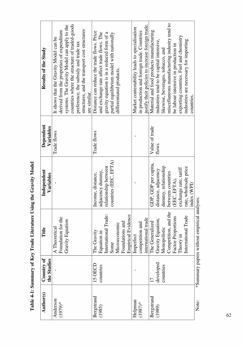
62
Tab
le 4
-1:
Su
mm
ary
of
Key
Tra
de
Lit
eratu
re U
sin
g t
he
Gra
vit
y M
od
el
Au
thor(
s)
Cou
ntr
y o
f th
e S
tud
ies
Tit
le
Ind
epen
den
t V
ari
ab
les
Dep
end
ent
Vari
ab
les
Res
ult
s of
the
Stu
dy
Ander
son
(1979)*
-
A T
heo
reti
cal
Foundat
ion f
or
the
Gra
vit
y E
quat
ion
- T
rade
flow
s It
show
s th
at t
he
Gra
vit
y M
odel
can
be
der
ived
fro
m t
he
pro
per
ties
of
expen
dit
ure
sy
stem
s. T
he
Gra
vit
y M
odel
can
apply
to t
he
countr
ies
wher
e th
e st
ruct
ure
of
trad
ed-g
oods
pre
fere
nce
, th
e su
bsi
dy a
nd t
rade
tax
st
ruct
ure
s, a
nd t
he
tran
sport
cost
str
uct
ure
s ar
e si
mil
ar.
Ber
gst
rand
(1985)
15 O
EC
D
countr
ies
The
Gra
vit
y
Equat
ion i
n
Inte
rnat
ional
Tra
de:
S
om
e M
icro
econom
ic
Foundat
ions
and
Em
pir
ical
Evid
ence
Inco
me,
dis
tance
, ad
jace
ncy
dum
my,
rela
tionsh
ip b
etw
een
countr
ies
(EE
C, E
FT
A)
Tra
de
flow
s D
ista
nce
can
red
uce
the
trad
e fl
ow
s. P
rice
an
d e
xch
ange
rate
aff
ect
trad
e fl
ow
s. T
he
gra
vit
y e
quat
ion i
s in
a r
educe
d f
orm
of
a par
tial
equil
ibri
um
model
wit
h n
atio
nal
ly
dif
fere
nti
ated
pro
duct
s.
Hel
pm
an
(1987)*
-
Imper
fect
co
mpet
itio
n a
nd
inte
rnat
ional
tra
de
- -
Mar
ket
conte
stab
ilit
y l
eads
to s
pec
iali
sati
on
in p
roduct
ion a
nd f
ore
ign
tra
de.
Countr
ies
just
ify t
hei
r poli
cies
to i
ncr
ease
fore
ign t
rade.
Ber
gst
rand
(1989)
17
dev
eloped
co
untr
ies
The
Gen
eral
ized
G
ravit
y E
quat
ion,
Monopoli
stic
C
om
pet
itio
n, an
d t
he
Fac
tor-
Pro
port
ions
Theo
ry i
n
Inte
rnat
ional
Tra
de
GD
P, G
DP
per
cap
ita,
dis
tance
, ad
jace
ncy
dum
my, re
lati
onsh
ip
bet
wee
n c
ountr
ies
(EE
C, E
FT
A),
ex
chan
ge
rate
, ta
riff
ra
te, w
hole
sale
pri
ce
index
(W
PI)
Val
ue
of
trad
e fl
ow
s M
ater
ial
and f
ood p
roduct
s m
anufa
cturi
ng
indust
ries
ten
d t
o b
e ca
pit
al i
nte
nsi
ve,
li
kew
ise,
bev
erag
es, to
bac
co, an
d
mis
cell
aneo
us
man
ufa
ctu
ring i
ndust
ry t
end t
o
be
labour
inte
nsi
ve
in p
roduct
ion i
n
export
ing c
ountr
ies.
Fu
el a
nd c
hem
istr
y
indust
ries
are
nec
essa
ry f
or
import
ing
countr
ies.
Note
: *S
um
mar
y p
aper
s w
itho
ut
empir
ical
anal
yse
s.
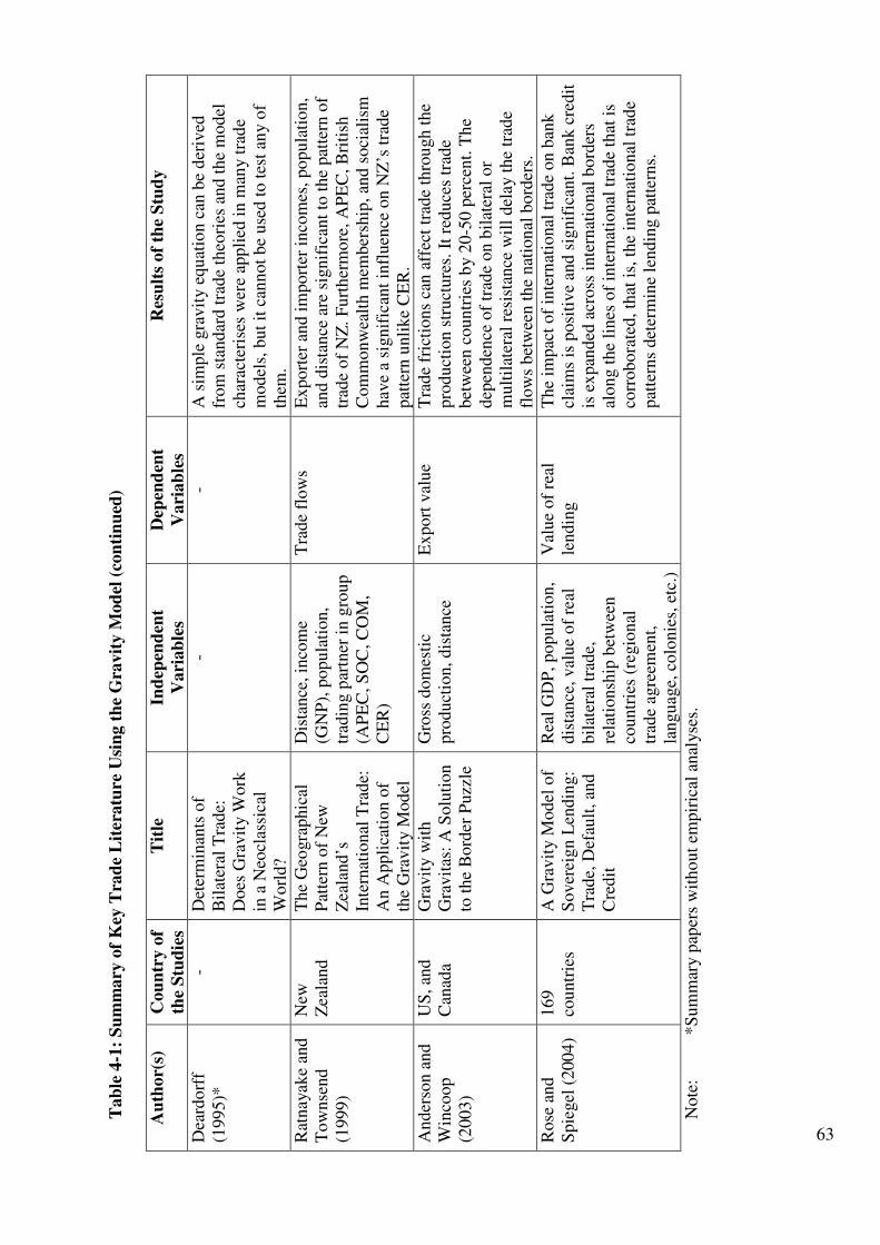
63
Tab
le 4
-1:
Su
mm
ary
of
Key
Tra
de
Lit
eratu
re U
sin
g t
he
Gra
vit
y M
od
el (
con
tin
ued
) Au
thor(
s)
Cou
ntr
y o
f th
e S
tud
ies
Tit
le
Ind
epen
den
t V
ari
ab
les
Dep
end
ent
Vari
ab
les
Res
ult
s of
the
Stu
dy
Dea
rdo
rff
(1995)*
-
Det
erm
inan
ts o
f B
ilat
eral
Tra
de:
D
oes
Gra
vit
y W
ork
in
a N
eocl
assi
cal
Worl
d?
- -
A s
imple
gra
vit
y e
quat
ion c
an b
e d
eriv
ed
from
sta
ndar
d t
rade
theo
ries
and t
he
model
ch
arac
teri
ses
wer
e ap
pli
ed i
n m
any t
rad
e m
odel
s, b
ut
it c
annot
be
use
d t
o t
est
any o
f th
em.
Rat
nay
ake
and
Tow
nse
nd
(1999)
New
Z
eala
nd
The
Geo
gra
phic
al
Pat
tern
of
New
Z
eala
nd’s
In
tern
atio
nal
Tra
de:
A
n A
ppli
cati
on o
f th
e G
ravit
y M
odel
Dis
tance
, in
com
e (G
NP
), p
opula
tion,
trad
ing p
artn
er i
n g
roup
(AP
EC
, S
OC
, C
OM
, C
ER
)
Tra
de
flow
s E
xport
er a
nd i
mport
er i
nco
mes
, popula
tion,
and d
ista
nce
are
sig
nif
ican
t to
the
pat
tern
of
trad
e of
NZ
. F
urt
her
more
, A
PE
C, B
riti
sh
Com
monw
ealt
h m
ember
ship
, an
d s
oci
alis
m
hav
e a
signif
ican
t in
fluen
ce o
n N
Z’s
tra
de
pat
tern
unli
ke
CE
R.
Ander
son a
nd
Win
coop
(2003)
US
, an
d
Can
ada
Gra
vit
y w
ith
Gra
vit
as:
A S
olu
tion
to t
he
Bord
er P
uzz
le
Gro
ss d
om
esti
c pro
duct
ion, dis
tance
E
xport
val
ue
Tra
de
fric
tions
can a
ffec
t tr
ade
thro
ugh t
he
pro
duct
ion s
truct
ure
s. I
t re
duce
s tr
ade
bet
wee
n c
ountr
ies
by 2
0-5
0 p
erce
nt.
Th
e dep
enden
ce o
f tr
ade
on b
ilat
eral
or
mult
ilat
eral
res
ista
nce
wil
l del
ay t
he
trad
e fl
ow
s bet
wee
n t
he
nat
ion
al b
ord
ers.
Rose
and
Spie
gel
(2004
) 169
countr
ies
A G
ravit
y M
odel
of
Sover
eign L
endin
g:
Tra
de,
Def
ault
, an
d
Cre
dit
Rea
l G
DP
, popula
tion,
dis
tance
, val
ue
of
real
bil
ater
al t
rade,
re
lati
onsh
ip b
etw
een
countr
ies
(reg
ional
tr
ade
agre
emen
t,
langu
age,
colo
nie
s, e
tc.)
Val
ue
of
real
le
ndin
g
The
impac
t of
inte
rnat
ional
tra
de
on b
ank
clai
ms
is p
osi
tive
and s
ignif
ican
t. B
ank c
redit
is
ex
pan
ded
acr
oss
inte
rnat
ional
bord
ers
along t
he
lines
of
inte
rnat
ional
tra
de
that
is
corr
obora
ted, th
at i
s, t
he
inte
rnat
ional
tra
de
pat
tern
s det
erm
ine
lendin
g p
atte
rns.
Note
: *S
um
mar
y p
aper
s w
itho
ut
empir
ical
anal
yse
s.
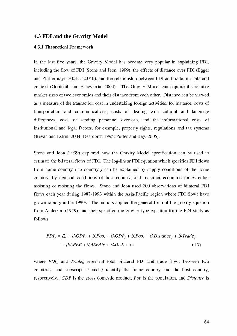
64
4.3 FDI and the Gravity Model
4.3.1 Theoretical Framework
In the last five years, the Gravity Model has become very popular in explaining FDI,
including the flow of FDI (Stone and Jeon, 1999), the effects of distance over FDI (Egger
and Pfaffermayr, 2004a, 2004b), and the relationship between FDI and trade in a bilateral
context (Gopinath and Echeverria, 2004). The Gravity Model can capture the relative
market sizes of two economies and their distance from each other. Distance can be viewed
as a measure of the transaction cost in undertaking foreign activities, for instance, costs of
transportation and communications, costs of dealing with cultural and language
differences, costs of sending personnel overseas, and the informational costs of
institutional and legal factors, for example, property rights, regulations and tax systems
(Bevan and Estrin, 2004; Deardorff, 1995; Portes and Rey, 2005).
Stone and Jeon (1999) explored how the Gravity Model specification can be used to
estimate the bilateral flows of FDI. The log-linear FDI equation which specifies FDI flows
from home country i to country j can be explained by supply conditions of the home
country, by demand conditions of host country, and by other economic forces either
assisting or resisting the flows. Stone and Jeon used 200 observations of bilateral FDI
flows each year during 1987-1993 within the Asia-Pacific region where FDI flows have
grown rapidly in the 1990s. The authors applied the general form of the gravity equation
from Anderson (1979), and then specified the gravity-type equation for the FDI study as
follows:
FDIij = β0 + β1GDPi + β2Popi + β3GDPj + β4Popj + β5Distanceij + β6Tradeij
+ β7APEC +β8ASEAN + β9DAE + εij (4.7)
where FDIij and Tradeij represent total bilateral FDI and trade flows between two
countries, and subscripts i and j identify the home country and the host country,
respectively. GDP is the gross domestic product, Pop is the population, and Distance is
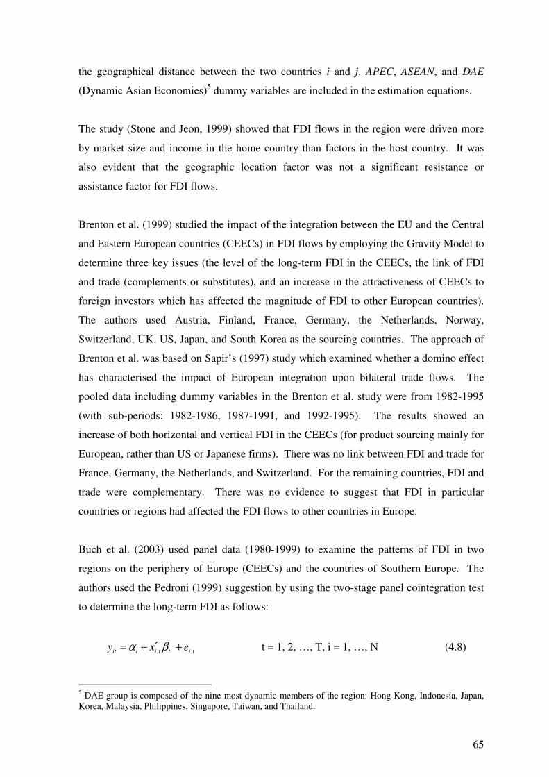
65
the geographical distance between the two countries i and j. APEC, ASEAN, and DAE
(Dynamic Asian Economies)5 dummy variables are included in the estimation equations.
The study (Stone and Jeon, 1999) showed that FDI flows in the region were driven more
by market size and income in the home country than factors in the host country. It was
also evident that the geographic location factor was not a significant resistance or
assistance factor for FDI flows.
Brenton et al. (1999) studied the impact of the integration between the EU and the Central
and Eastern European countries (CEECs) in FDI flows by employing the Gravity Model to
determine three key issues (the level of the long-term FDI in the CEECs, the link of FDI
and trade (complements or substitutes), and an increase in the attractiveness of CEECs to
foreign investors which has affected the magnitude of FDI to other European countries).
The authors used Austria, Finland, France, Germany, the Netherlands, Norway,
Switzerland, UK, US, Japan, and South Korea as the sourcing countries. The approach of
Brenton et al. was based on Sapir’s (1997) study which examined whether a domino effect
has characterised the impact of European integration upon bilateral trade flows. The
pooled data including dummy variables in the Brenton et al. study were from 1982-1995
(with sub-periods: 1982-1986, 1987-1991, and 1992-1995). The results showed an
increase of both horizontal and vertical FDI in the CEECs (for product sourcing mainly for
European, rather than US or Japanese firms). There was no link between FDI and trade for
France, Germany, the Netherlands, and Switzerland. For the remaining countries, FDI and
trade were complementary. There was no evidence to suggest that FDI in particular
countries or regions had affected the FDI flows to other countries in Europe.
Buch et al. (2003) used panel data (1980-1999) to examine the patterns of FDI in two
regions on the periphery of Europe (CEECs) and the countries of Southern Europe. The
authors used the Pedroni (1999) suggestion by using the two-stage panel cointegration test
to determine the long-term FDI as follows:
tittiiit exy ,, +′+= βα t = 1, 2, …, T, i = 1, …, N (4.8)
5 DAE group is composed of the nine most dynamic members of the region: Hong Kong, Indonesia, Japan, Korea, Malaysia, Philippines, Singapore, Taiwan, and Thailand.
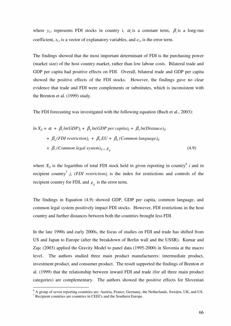
66
where yi,t represents FDI stocks in country i, iα is a constant term, iβ is a long-run
coefficient, xi,t is a vector of explanatory variables, and ei,t is the error term.
The findings showed that the most important determinant of FDI is the purchasing power
(market size) of the host country market, rather than low labour costs. Bilateral trade and
GDP per capita had positive effects on FDI. Overall, bilateral trade and GDP per capita
showed the positive effects of the FDI stocks. However, the findings gave no clear
evidence that trade and FDI were complements or substitutes, which is inconsistent with
the Brenton et al. (1999) study.
The FDI forecasting was investigated with the following equation (Buch et al., 2003):
ln Xij = α + 1β ln(GDP)j + 2β ln(GDP per capita)j + 3β ln(Distance)ij
+ 4β (FDI restriction)j + 5β EU + 6β (Common language)ij
+ 7β (Common legal system)ij + ijε (4.9)
where Xij is the logarithm of total FDI stock held in given reporting in country6 i and in
recipient country7 j, (FDI restriction)j is the index for restrictions and controls of the
recipient country for FDI, and ijε is the error term.
The findings in Equation (4.9) showed GDP, GDP per capita, common language, and
common legal system positively impact FDI stocks. However, FDI restrictions in the host
country and further distances between both the countries brought less FDI.
In the late 1990s and early 2000s, the focus of studies on FDI and trade has shifted from
US and Japan to Europe (after the breakdown of Berlin wall and the USSR). Kumar and
Zajc (2003) applied the Gravity Model to panel data (1995-2000) in Slovenia at the macro
level. The authors studied three main product manufacturers: intermediate product,
investment product, and consumer product. The result supported the findings of Brenton et
al. (1999) that the relationship between inward FDI and trade (for all three main product
categories) are complementary. The authors showed the positive effects for Slovenian
6 A group of seven reporting countries are: Austria, France, Germany, the Netherlands, Sweden, UK, and US. 7 Recipient countries are countries in CEECs and the Southern Europe.
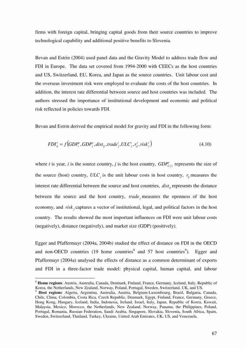
67
firms with foreign capital, bringing capital goods from their source countries to improve
technological capability and additional positive benefits to Slovenia.
Bevan and Estrin (2004) used panel data and the Gravity Model to address trade flow and
FDI in Europe. The data set covered from 1994-2000 with CEECs as the host countries
and US, Switzerland, EU, Korea, and Japan as the source countries. Unit labour cost and
the overseas investment risk were employed to evaluate the costs of the host countries. In
addition, the interest rate differential between source and host countries was included. The
authors stressed the importance of institutional development and economic and political
risk reflected in policies towards FDI.
Bevan and Estrin derived the empirical model for gravity and FDI in the following form:
( )t
j
t
ij
t
j
t
jij
t
j
t
i
t
ij riskrULCtradedistGDPGDPfFDI ,,,,,,= (4.10)
where t is year, i is the source country, j is the host country, t
jiGDP )( represents the size of
the source (host) country, jULC is the unit labour costs in host country, ijr measures the
interest rate differential between the source and host countries, ijdist represents the distance
between the source and the host country, jtrade measures the openness of the host
economy, and jrisk captures a vector of institutional, legal, and political factors in the host
country. The results showed the most important influences on FDI were unit labour costs
(negatively), distance (negatively), and market size (GDP) (positively).
Egger and Pfaffermayr (2004a, 2004b) studied the effect of distance on FDI in the OECD
and non-OECD countries (19 home countries8 and 57 host countries9). Egger and
Pfaffermayr (2004a) analysed the effects of distance as a common determinant of exports
and FDI in a three-factor trade model: physical capital, human capital, and labour
8 Home regions: Austria, Australia, Canada, Denmark, Finland, France, Germany, Iceland, Italy, Republic of Korea, the Netherlands, New Zealand, Norway, Poland, Portugal, Sweden, Switzerland, UK, and US. 9 Host regions: Algeria, Argentina, Australia, Austria, Belgium-Luxembourg, Brazil, Bulgaria, Canada, Chile, China, Colombia, Costa Rica, Czech Republic, Denmark, Egypt, Finland, France, Germany, Greece, Hong Kong, Hungary, Iceland, India, Indonesia, Ireland, Israel, Italy, Japan, Republic of Korea, Kuwait, Malaysia, Mexico, Morocco, the Netherlands, New Zealand, Norway, Panama, the Philippines, Poland, Portugal, Romania, Russian Federation, Saudi Arabia, Singapore, Slovakia, Slovenia, South Africa, Spain, Sweden, Switzerland, Thailand, Turkey, Ukraine, United Arab Emirates, UK, US, and Venezuela.
68
endowment; assuming that distance affected both pure trade costs and plant set-up costs.
They considered the CES utility function and the balance of payments guaranteed that
goods trade flows were balanced by both trade in invisibles and capital flows across
borders (FDI). The results showed the impact of distance depended on the relative
importance of fixed foreign plant set-up costs compared to trade costs. Distance had a
significantly weaker effect on plant set-up costs than on exports. Exports and FDI were
not necessarily substitutes with respect to distance since the predicted impact depended on
its importance for fixed plant set-up costs relative to transportation costs and the relative
importance of firms. The results were similar to Bevan and Estrin (2004) findings. There
were significant negative interactions between distance and the difference in physical
capital to labour ratio on outward FDI.
Egger and Pfaffermayr (2004b) used OECD panel data on stocks of outward FDI to
evaluate the impact of bilateral investment treaties. The authors concentrated on FDI and
analysed whether bilateral real outward FDI stocks rose as new treaties were signed or
implemented. The finding showed a positive significant impact of bilateral investment
treaties (BITs) on bilateral FDI stocks. To check the robustness of findings and to examine
an endogenous treatment of BITs, the authors added infrastructure variables, corporate tax
rates, and trading bloc effects to ensure that the estimated BITs coefficients did not include
effects from other omitted variables. However, the alternative results did not change the
estimated BITs but estimated the BITs more robustly. It implied that bilateral investment
treaties reduce barriers to FDI.
Gopinath and Echeverria (2004) examined the relationship between FDI and trade in a
bilateral context using a Gravity Model approach. The relative demand (import/FDI-
produced goods) was negatively affected by tariffs and transportation cost and positively
affected by institutional distance. The results suggest that, as distance between the two
economies increases, the home country’s bilateral exports (host country’s bilateral imports)
fall relative to FDI-based production. Hence, the authors reported geographical distance
caused countries to switch from nominal trade to FDI, which has not been evidenced in
previous studies before.
69
The Gravity Model has also been used to examine cross border equity flows (Portes and
Rey, 2005). Portes and Rey explored eight years of panel data (1989-1996) on bilateral
cross border equity flows between 14 regions (US, Japan, UK, Germany, France,
Switzerland, the Netherlands, Spain, Italy, Scandinavia, Canada, Australia, Hong Kong,
and Singapore). The authors included variables such as the information flows, transactions
technology, and time into the empirical model.
The results showed that distance was a significantly negative factor. Telephone calls and
financial market sophistication had a positive influence on transaction flows. The cross
border equity flows and trading costs relied on market size in the source and destination
countries. However, there was weak evidence to support that cross border equity flows
were purely complementary to trade. The authors suggested that the model may capture
some determinants of asset flows but not all.
Table 4-2 presents a summary of the key FDI literature using the Gravity Model. These
studies have been discussed in Section 4.3.1.
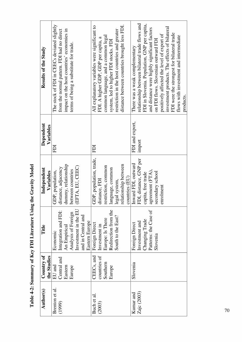
70
Tab
le 4
-2:
Su
mm
ary
of
Key
FD
I L
iter
atu
re U
sin
g t
he
Gra
vit
y M
od
el
Au
thor(
s)
Cou
ntr
y o
f th
e S
tud
ies
Tit
le
Ind
epen
den
t V
ari
ab
les
Dep
end
ent
Vari
ab
les
Res
ult
s of
the
Stu
dy
Bre
nto
n e
t al
. (1
999)
EU
and
Cen
tral
and
Eas
tern
E
uro
pe
Eco
nom
ic
Inte
gra
tion a
nd F
DI:
A
n E
mpir
ical
A
nal
ysi
s of
Fore
ign
Inv
estm
ent
in t
he
EU
an
d i
n C
entr
al a
nd
Eas
tern
Euro
pe
GD
P, popula
tion,
dis
tance
, ad
jace
ncy
dum
my, re
lati
onsh
ip
bet
wee
n c
ountr
ies
(EF
TA
, E
U, C
EE
C)
FD
I T
he
stock
of
FD
I in
CE
EC
s dev
iate
d s
lightl
y
from
the
norm
al p
atte
rn.
FD
I h
ad n
o d
irec
t im
pac
t on t
he
host
countr
ies’
eco
nom
ies
in
term
s of
bei
ng a
subst
itute
for
trad
e.
Buch
et
al.
(2003)
CE
EC
s, a
nd
countr
ies
of
South
ern
Euro
pe
Fore
ign D
irec
t In
ves
tmen
t in
E
uro
pe:
Is
Ther
e R
edir
ecti
on f
rom
the
South
to t
he
Eas
t?
GD
P, popula
tion, tr
ade,
dis
tance
, F
DI
rest
rict
ion, co
mm
on
langu
age,
com
mon
legal
syst
em,
rela
tionsh
ip b
etw
een
countr
ies
(EU
)
FD
I A
ll e
xpla
nat
ory
var
iable
s w
ere
signif
ican
t to
F
DI.
A h
igh
er G
DP
, G
DP
per
cap
ita,
a
com
mon l
angu
age,
and a
com
mon l
egal
sy
stem
, le
d t
o h
igher
FD
I st
ock
s. F
DI
rest
rict
ion i
n t
he
host
cou
ntr
ies
and g
reat
er
dis
tance
bet
wee
n c
ountr
ies
bro
ught
less
FD
I.
Kum
ar a
nd
Zaj
c (2
003)
Slo
ven
ia
Fore
ign D
irec
t In
ves
tmen
t an
d
Chan
gin
g T
rade
Pat
tern
s: t
he
Cas
e of
Slo
ven
ia
Inw
ard F
DI,
outw
ard
FD
I, d
ista
nce
, G
NP
per
ca
pit
a, f
ree
trad
e ag
reem
ent
(FT
A),
se
condar
y s
chool
enro
lmen
t
FD
I an
d e
xport
, im
port
T
her
e w
as a
wea
k c
om
ple
men
tary
re
lati
onsh
ip b
etw
een b
ilat
eral
tra
de
flow
s an
d
FD
I in
Slo
ven
ia. P
opula
tion, G
NP
per
cap
ita,
an
d d
ista
nce
wer
e hig
hly
sig
nif
ican
t fa
ctors
on F
DI
flow
s. S
loven
ian o
utw
ard F
DI
posi
tivel
y af
fect
ed t
he
level
of
export
of
inves
tmen
t pro
duct
s. T
he
effe
cts
of
bil
ater
al
FD
I w
ere
the
stro
nges
t fo
r bil
ater
al t
rad
e fl
ow
s w
ith i
nves
tmen
t an
d i
nte
rmed
iate
pro
duct
s.
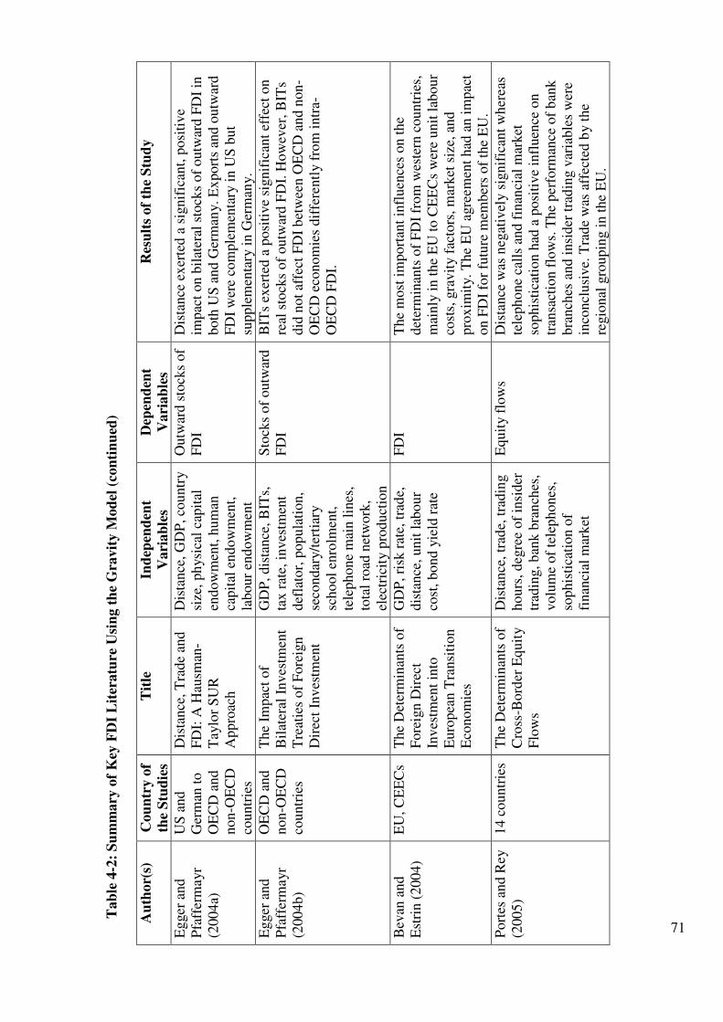
71
Tab
le 4
-2:
Su
mm
ary
of
Key
FD
I L
iter
atu
re U
sin
g t
he
Gra
vit
y M
od
el (
con
tin
ued
) Au
thor(
s)
Cou
ntr
y o
f th
e S
tud
ies
Tit
le
Ind
epen
den
t V
ari
ab
les
Dep
end
ent
Vari
ab
les
Res
ult
s of
the
Stu
dy
Egger
and
Pfa
ffer
may
r (2
004a)
US
and
Ger
man
to
OE
CD
and
non-O
EC
D
countr
ies
Dis
tance
, T
rade
and
FD
I: A
Hau
sman
-T
aylo
r S
UR
A
ppro
ach
Dis
tance
, G
DP
, co
untr
y
size
, ph
ysic
al c
apit
al
endow
men
t, h
um
an
capit
al e
ndow
men
t,
labour
endow
men
t
Outw
ard s
tock
s of
FD
I
Dis
tance
ex
erte
d a
sig
nif
ican
t, p
osi
tive
impac
t on b
ilat
eral
sto
cks
of
outw
ard F
DI
in
both
US
and G
erm
any. E
xport
s an
d o
utw
ard
FD
I w
ere
com
ple
men
tary
in U
S b
ut
supple
men
tary
in G
erm
any.
Egger
and
Pfa
ffer
may
r (2
004b)
OE
CD
and
non-O
EC
D
countr
ies
The
Impac
t of
Bil
ater
al I
nves
tmen
t T
reat
ies
of
Fore
ign
Dir
ect
Inv
estm
ent
GD
P, dis
tance
, B
ITs,
ta
x r
ate,
inves
tmen
t def
lato
r, p
opula
tion,
seco
ndar
y/t
erti
ary
school
enro
lmen
t,
tele
phone
mai
n l
ines
, to
tal
road
net
work
, el
ectr
icit
y p
roduct
ion
Sto
cks
of
outw
ard
FD
I B
ITs
exer
ted a
posi
tive
signif
ican
t ef
fect
on
real
sto
cks
of
outw
ard F
DI.
How
ever
, B
ITs
did
not
affe
ct F
DI
bet
wee
n O
EC
D a
nd n
on-
OE
CD
eco
nom
ies
dif
fere
ntl
y f
rom
intr
a-O
EC
D F
DI.
Bev
an a
nd
Est
rin (
2004)
EU
, C
EE
Cs
The
Det
erm
inan
ts o
f F
ore
ign D
irec
t In
ves
tmen
t in
to
Euro
pea
n T
ransi
tion
Eco
nom
ies
GD
P, ri
sk r
ate,
tra
de,
dis
tance
, unit
lab
our
cost
, bond y
ield
rat
e
FD
I T
he
most
im
port
ant
infl
uen
ces
on t
he
det
erm
inan
ts o
f F
DI
fro
m w
este
rn c
ountr
ies,
m
ainly
in t
he
EU
to C
EE
Cs
wer
e unit
lab
our
cost
s, g
ravit
y f
acto
rs, m
arket
siz
e, a
nd
pro
xim
ity.
The
EU
agre
emen
t had
an i
mpac
t on F
DI
for
futu
re m
ember
s of
the
EU
.
Port
es a
nd R
ey
(2005)
14 c
ountr
ies
T
he
Det
erm
inan
ts o
f C
ross
-Bord
er E
quit
y
Flo
ws
Dis
tance
, tr
ade,
tra
din
g
hours
, deg
ree
of
insi
der
tr
adin
g, b
ank b
ran
ches
, volu
me
of
tele
phones
, so
phis
tica
tion o
f fi
nan
cial
mar
ket
Equit
y f
low
s D
ista
nce
was
neg
ativ
ely s
ignif
ican
t w
her
eas
tele
phone
call
s an
d f
inan
cial
mar
ket
so
phis
tica
tion h
ad a
posi
tive
infl
uen
ce o
n
tran
sact
ion f
low
s. T
he
per
form
ance
of
ban
k
bra
nch
es a
nd i
nsi
der
tra
din
g v
aria
ble
s w
ere
inco
ncl
usi
ve.
Tra
de
was
aff
ecte
d b
y t
he
regio
nal
gro
upin
g i
n t
he
EU
.
72
4.4 Summary
The Gravity Model was developed from the Newton’s Law of Gravitation to predict the
movement of information and commodities between two different places. The Gravity
Model can be used in trade and FDI studies. Earlier researchers used the Gravity Model to
test the factors of trade between two countries. It is a model that proved to be applicable
and empirically successful in explaining bilateral trade flows. The model appears to be
proportional to GDPs and negatively linked to geographical distance. The model was
applied to various goods and factors (such as income and population) moving over
regional/national/economic borders. It described the flow from an origin i to a destination
j in terms of supply factors in the origin, demand factors in the destination and various
interesting or retraining factors relating to the specific flow, such as distance (as a proxy
for trade costs) and trade preferences (Anderson, 1979).
Since the growth of FDI in recent decades shares some features with the evolution of trade,
having become more intense between countries with similar and relatively high income
levels, and having grown faster than income, the Gravity Model may also be useful in
modelling the regional pattern of FDI (Brenton et al., 1999). More recently, the Gravity
Model has been one of the most influential methods to analyse countries’ attractiveness as
a location for FDI using aggregate-level data or identifying the determinants of FDI across
countries.
Distance, incomes, and population were evaluated using the Gravity Model in many
empirical studies (Anderson, 1979; Bergstrand, 1985; McCallum, 1995). However, some
researchers added significant variables into the empirical model such as the transport costs,
labour costs, exchange rate, price, regional grouping to test the hypotheses (Buch et al.,
2003; Ratnayake and Townsend, 1999; Stone and Jeon, 1999). In addition, many potential
factors (from many of trade and investment theories) were added into the empirical gravity
patterns. The Gravity Model can be flexible and further developed to answer the
researchers’ questions and propositions on trade and FDI studies.
The following chapter discusses the methodology and empirical equations using the
Gravity Model.
CHAPTER 5
EMPIRICAL MODELS AND METHODOLOGY This chapter discusses the variables used in the extended Gravity Model. This is followed
by a description of the empirical model and technique used to determine the FDI and
equity flows to Thailand. One-way and two-way error component models are also
discussed in this section. Section 5.3 discusses the extended Gravity Model in detail and
the model specification with hypothesised signs. Section 5.4 discusses the data sources
used in this research. The structural break test that was used to test the effects of the 1997
Asian Financial Crisis on FDI and equity flows to Thailand is discussed in Section 5.5.
Section 5.6 presents the SURE model to examine and analyse the relationship between FDI
and industrial categories across Thailand.
5.1 Summary of Variables Used in the Gravity Model
The extended Gravity Model provides a wealth of potential instrumental variables. It is
widely used to solve the problems of investment and international trade (Bougheas et al.,
1999; Pelletiere and Reinert, 2004; Ratnayake and Townsend, 1999). Researchers have
attempted to investigate whether border effects inhibit foreign investment and international
trade using the Gravity Model. Moreover, Markusen and Maskus (2002) argued that the
Gravity Model can be used to discriminate between alternative trade theories and adjusted
to a pattern of investment flows. This study develops a theoretical Gravity Model to
answer the research objectives, and to test the determinants of FDI and FPI in Thailand.
Empirical studies of bilateral FDI flows using the Gravity Model have been based on the
proposition that transactions between regions are determined by their national incomes
(such as GDP, GDP per capita, GNP) and their geographical distance. Table 5-1 presents a
summary of the variables generally used in the Gravity Model. These were discussed in
Chapter 4.
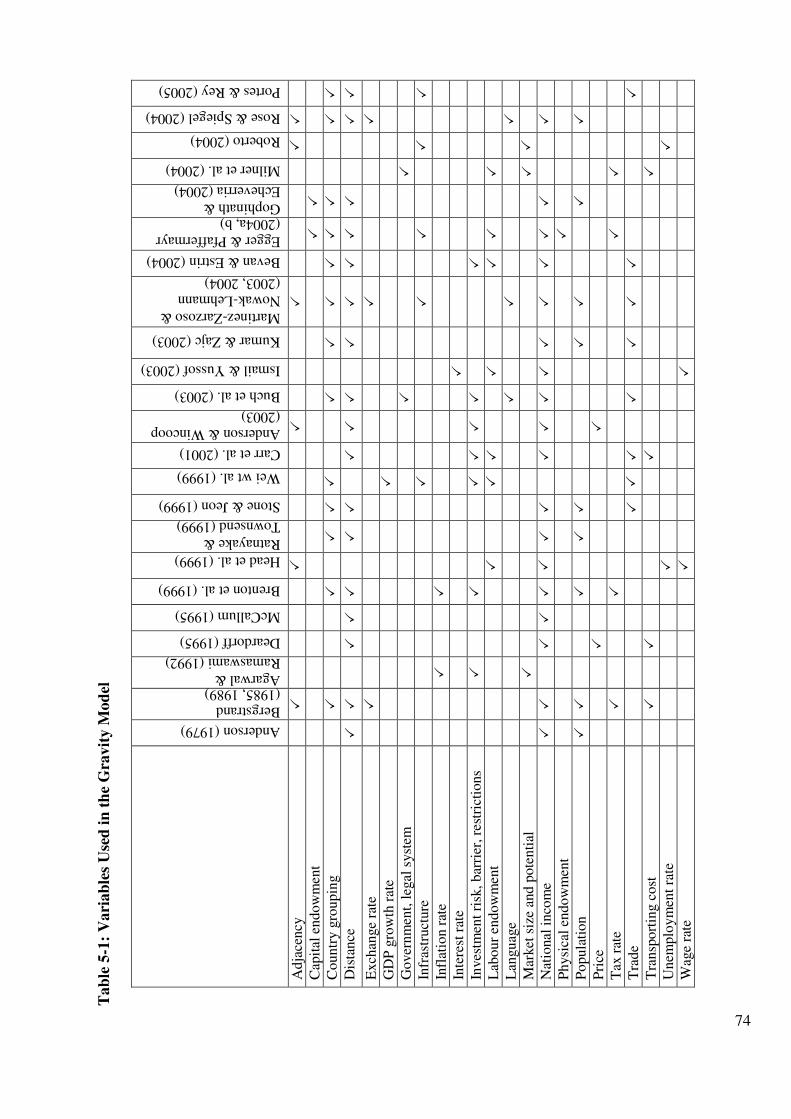
74
Tab
le 5
-1:
Vari
ab
les
Use
d i
n t
he
Gra
vit
y M
od
el
Anderson (1979)
Bergstrand (1985, 1989) Agarwal & Ramaswami (1992)
Deardorff (1995)
McCallum (1995)
Brenton et al. (1999)
Head et al. (1999)
Ratnayake &
Townsend (1999)
Stone & Jeon (1999)
Wei wt al. (1999)
Carr et al. (2001)
Anderson & Wincoop
(2003)
Buch et al. (2003)
Ismail & Yussof (2003)
Kumar & Zajc (2003)
Martinez-Zarzoso & Nowak-Lehmann (2003, 2004)
Bevan & Estrin (2004)
Egger & Pfaffermayr (2004a, b) Gophinath & Echeverria (2004)
Milner et al. (2004)
Roberto (2004)
Rose & Spiegel (2004)
Portes & Rey (2005)
Adja
cency
�
�
�
�
�
�
Cap
ital
endow
men
t
�
�
Countr
y g
roupin
g
�
�
�
�
�
�
�
�
�
�
�
�
�
Dis
tance
�
�
�
�
�
�
�
�
�
�
�
�
�
�
�
�
�
Exch
ange
rate
�
�
�
GD
P g
row
th r
ate
�
Gover
nm
ent,
leg
al s
yst
em
�
�
Infr
astr
uct
ure
�
�
�
�
�
Infl
atio
n r
ate
�
�
Inte
rest
rat
e
�
Inves
tmen
t ri
sk, bar
rier
, re
stri
ctio
ns
�
�
�
�
�
�
�
Lab
our
endow
men
t
�
�
�
�
�
�
�
Lan
guag
e
�
�
�
Mar
ket
siz
e an
d p
ote
nti
al
�
�
�
Nat
ional
inco
me
�
�
�
�
�
�
�
�
�
�
�
�
�
�
�
�
�
�
Physi
cal
endow
men
t
�
Popula
tion
�
�
�
�
�
�
�
�
�
Pri
ce
�
�
Tax
rat
e
�
�
�
�
Tra
de
�
�
�
�
�
�
�
�
Tra
nsp
ort
ing c
ost
�
�
�
�
Unem
plo
ym
ent
rate
�
�
Wag
e ra
te
�
�
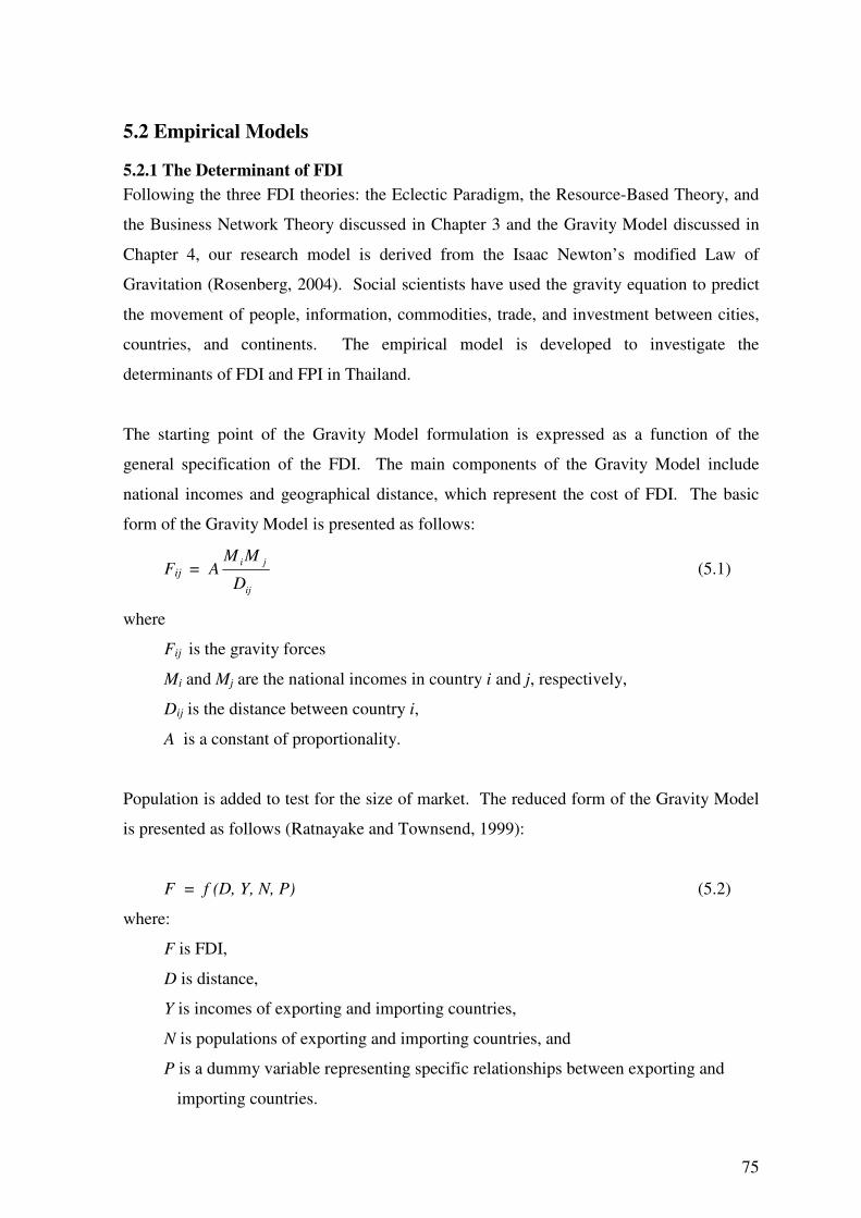
75
5.2 Empirical Models
5.2.1 The Determinant of FDI
Following the three FDI theories: the Eclectic Paradigm, the Resource-Based Theory, and
the Business Network Theory discussed in Chapter 3 and the Gravity Model discussed in
Chapter 4, our research model is derived from the Isaac Newton’s modified Law of
Gravitation (Rosenberg, 2004). Social scientists have used the gravity equation to predict
the movement of people, information, commodities, trade, and investment between cities,
countries, and continents. The empirical model is developed to investigate the
determinants of FDI and FPI in Thailand.
The starting point of the Gravity Model formulation is expressed as a function of the
general specification of the FDI. The main components of the Gravity Model include
national incomes and geographical distance, which represent the cost of FDI. The basic
form of the Gravity Model is presented as follows:
Fij = Aij
ji
D
MM (5.1)
where
Fij is the gravity forces
Mi and Mj are the national incomes in country i and j, respectively,
Dij is the distance between country i,
A is a constant of proportionality.
Population is added to test for the size of market. The reduced form of the Gravity Model
is presented as follows (Ratnayake and Townsend, 1999):
F = f (D, Y, N, P) (5.2)
where:
F is FDI,
D is distance,
Y is incomes of exporting and importing countries,
N is populations of exporting and importing countries, and
P is a dummy variable representing specific relationships between exporting and
importing countries.
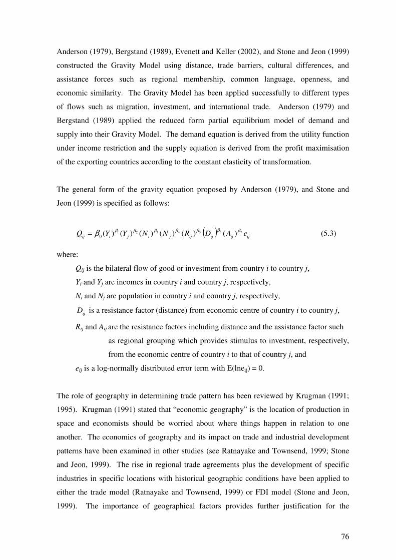
76
Anderson (1979), Bergstand (1989), Evenett and Keller (2002), and Stone and Jeon (1999)
constructed the Gravity Model using distance, trade barriers, cultural differences, and
assistance forces such as regional membership, common language, openness, and
economic similarity. The Gravity Model has been applied successfully to different types
of flows such as migration, investment, and international trade. Anderson (1979) and
Bergstand (1989) applied the reduced form partial equilibrium model of demand and
supply into their Gravity Model. The demand equation is derived from the utility function
under income restriction and the supply equation is derived from the profit maximisation
of the exporting countries according to the constant elasticity of transformation.
The general form of the gravity equation proposed by Anderson (1979), and Stone and
Jeon (1999) is specified as follows:
( )ijijijijjijiij eADRNNYYQ 7654321 )()()()()()(0
ββββββββ= (5.3)
where:
Qij is the bilateral flow of good or investment from country i to country j,
Yi and Yj are incomes in country i and country j, respectively,
Ni and Nj are population in country i and country j, respectively,
ijD is a resistance factor (distance) from economic centre of country i to country j,
Rij and Aij are the resistance factors including distance and the assistance factor such
as regional grouping which provides stimulus to investment, respectively,
from the economic centre of country i to that of country j, and
eij is a log-normally distributed error term with E(lneij) = 0.
The role of geography in determining trade pattern has been reviewed by Krugman (1991;
1995). Krugman (1991) stated that “economic geography” is the location of production in
space and economists should be worried about where things happen in relation to one
another. The economics of geography and its impact on trade and industrial development
patterns have been examined in other studies (see Ratnayake and Townsend, 1999; Stone
and Jeon, 1999). The rise in regional trade agreements plus the development of specific
industries in specific locations with historical geographic conditions have been applied to
either the trade model (Ratnayake and Townsend, 1999) or FDI model (Stone and Jeon,
1999). The importance of geographical factors provides further justification for the
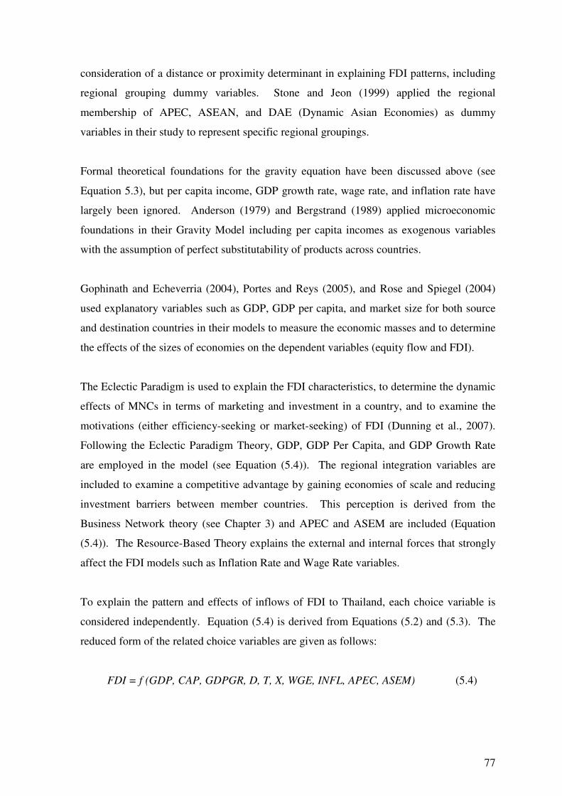
77
consideration of a distance or proximity determinant in explaining FDI patterns, including
regional grouping dummy variables. Stone and Jeon (1999) applied the regional
membership of APEC, ASEAN, and DAE (Dynamic Asian Economies) as dummy
variables in their study to represent specific regional groupings.
Formal theoretical foundations for the gravity equation have been discussed above (see
Equation 5.3), but per capita income, GDP growth rate, wage rate, and inflation rate have
largely been ignored. Anderson (1979) and Bergstrand (1989) applied microeconomic
foundations in their Gravity Model including per capita incomes as exogenous variables
with the assumption of perfect substitutability of products across countries.
Gophinath and Echeverria (2004), Portes and Reys (2005), and Rose and Spiegel (2004)
used explanatory variables such as GDP, GDP per capita, and market size for both source
and destination countries in their models to measure the economic masses and to determine
the effects of the sizes of economies on the dependent variables (equity flow and FDI).
The Eclectic Paradigm is used to explain the FDI characteristics, to determine the dynamic
effects of MNCs in terms of marketing and investment in a country, and to examine the
motivations (either efficiency-seeking or market-seeking) of FDI (Dunning et al., 2007).
Following the Eclectic Paradigm Theory, GDP, GDP Per Capita, and GDP Growth Rate
are employed in the model (see Equation (5.4)). The regional integration variables are
included to examine a competitive advantage by gaining economies of scale and reducing
investment barriers between member countries. This perception is derived from the
Business Network theory (see Chapter 3) and APEC and ASEM are included (Equation
(5.4)). The Resource-Based Theory explains the external and internal forces that strongly
affect the FDI models such as Inflation Rate and Wage Rate variables.
To explain the pattern and effects of inflows of FDI to Thailand, each choice variable is
considered independently. Equation (5.4) is derived from Equations (5.2) and (5.3). The
reduced form of the related choice variables are given as follows:
FDI = f (GDP, CAP, GDPGR, D, T, X, WGE, INFL, APEC, ASEM) (5.4)
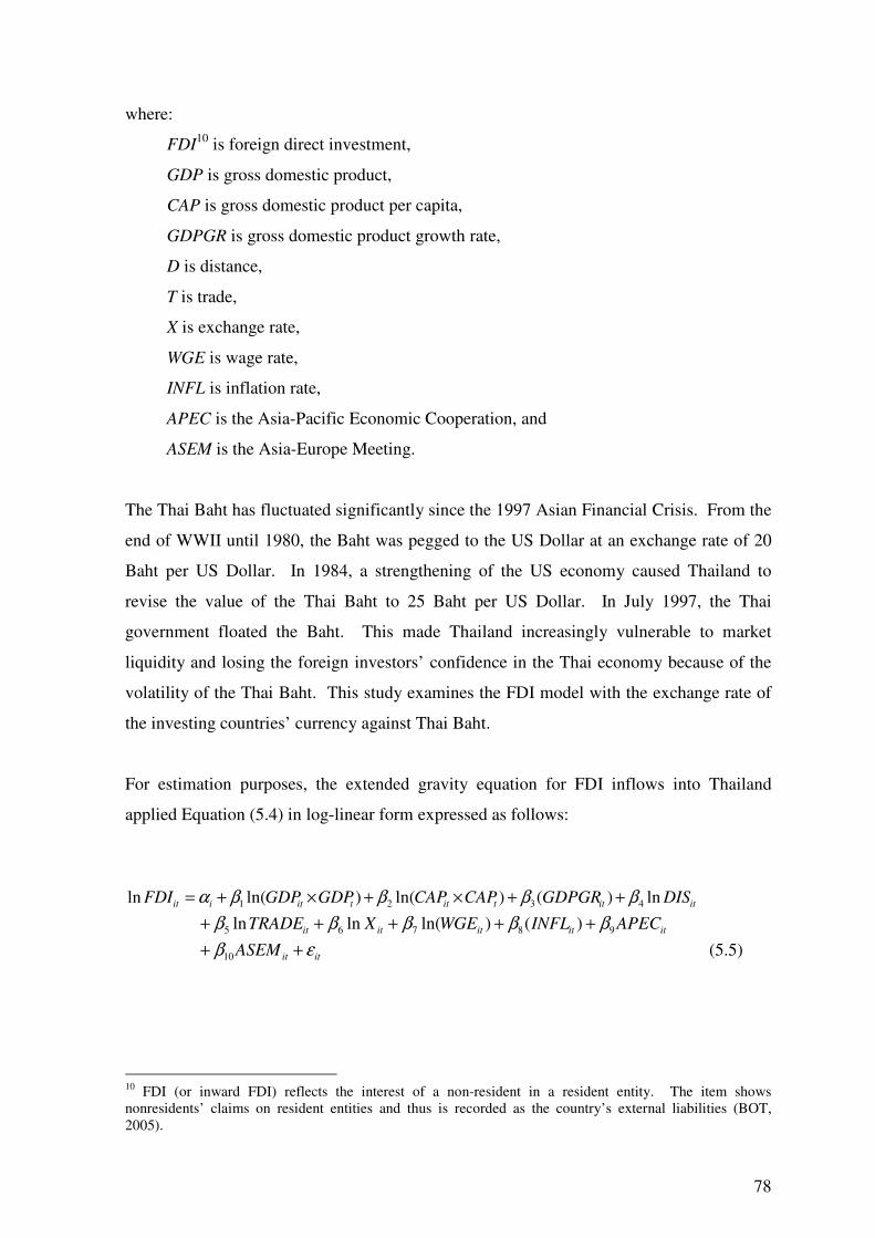
78
where:
FDI10 is foreign direct investment,
GDP is gross domestic product,
CAP is gross domestic product per capita,
GDPGR is gross domestic product growth rate,
D is distance,
T is trade,
X is exchange rate,
WGE is wage rate,
INFL is inflation rate,
APEC is the Asia-Pacific Economic Cooperation, and
ASEM is the Asia-Europe Meeting.
The Thai Baht has fluctuated significantly since the 1997 Asian Financial Crisis. From the
end of WWII until 1980, the Baht was pegged to the US Dollar at an exchange rate of 20
Baht per US Dollar. In 1984, a strengthening of the US economy caused Thailand to
revise the value of the Thai Baht to 25 Baht per US Dollar. In July 1997, the Thai
government floated the Baht. This made Thailand increasingly vulnerable to market
liquidity and losing the foreign investors’ confidence in the Thai economy because of the
volatility of the Thai Baht. This study examines the FDI model with the exchange rate of
the investing countries’ currency against Thai Baht.
For estimation purposes, the extended gravity equation for FDI inflows into Thailand
applied Equation (5.4) in log-linear form expressed as follows:
itittittitiit DISGDPGRCAPCAPGDPGDPFDI ln)()ln()ln(ln 4321 ββββα ++×+×+=
ititititit APECINFLWGEXTRADE 98765 )()ln(lnln βββββ +++++
ititASEM εβ ++ 10 (5.5)
10 FDI (or inward FDI) reflects the interest of a non-resident in a resident entity. The item shows nonresidents’ claims on resident entities and thus is recorded as the country’s external liabilities (BOT, 2005).
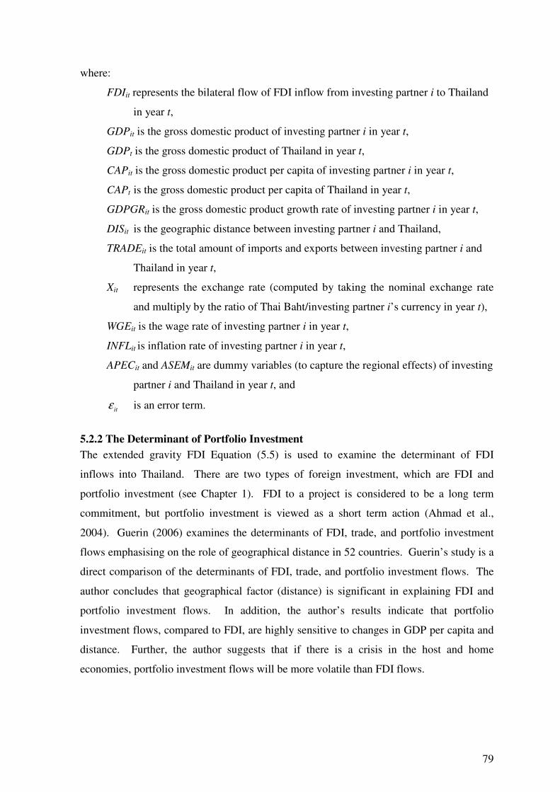
79
where:
FDIit represents the bilateral flow of FDI inflow from investing partner i to Thailand
in year t,
GDPit is the gross domestic product of investing partner i in year t,
GDPt is the gross domestic product of Thailand in year t,
CAPit is the gross domestic product per capita of investing partner i in year t,
CAPt is the gross domestic product per capita of Thailand in year t,
GDPGRit is the gross domestic product growth rate of investing partner i in year t,
DISit is the geographic distance between investing partner i and Thailand,
TRADEit is the total amount of imports and exports between investing partner i and
Thailand in year t,
Xit represents the exchange rate (computed by taking the nominal exchange rate
and multiply by the ratio of Thai Baht/investing partner i’s currency in year t),
WGEit is the wage rate of investing partner i in year t,
INFLit is inflation rate of investing partner i in year t,
APECit and ASEMit are dummy variables (to capture the regional effects) of investing
partner i and Thailand in year t, and
itε is an error term.
5.2.2 The Determinant of Portfolio Investment
The extended gravity FDI Equation (5.5) is used to examine the determinant of FDI
inflows into Thailand. There are two types of foreign investment, which are FDI and
portfolio investment (see Chapter 1). FDI to a project is considered to be a long term
commitment, but portfolio investment is viewed as a short term action (Ahmad et al.,
2004). Guerin (2006) examines the determinants of FDI, trade, and portfolio investment
flows emphasising on the role of geographical distance in 52 countries. Guerin’s study is a
direct comparison of the determinants of FDI, trade, and portfolio investment flows. The
author concludes that geographical factor (distance) is significant in explaining FDI and
portfolio investment flows. In addition, the author’s results indicate that portfolio
investment flows, compared to FDI, are highly sensitive to changes in GDP per capita and
distance. Further, the author suggests that if there is a crisis in the host and home
economies, portfolio investment flows will be more volatile than FDI flows.
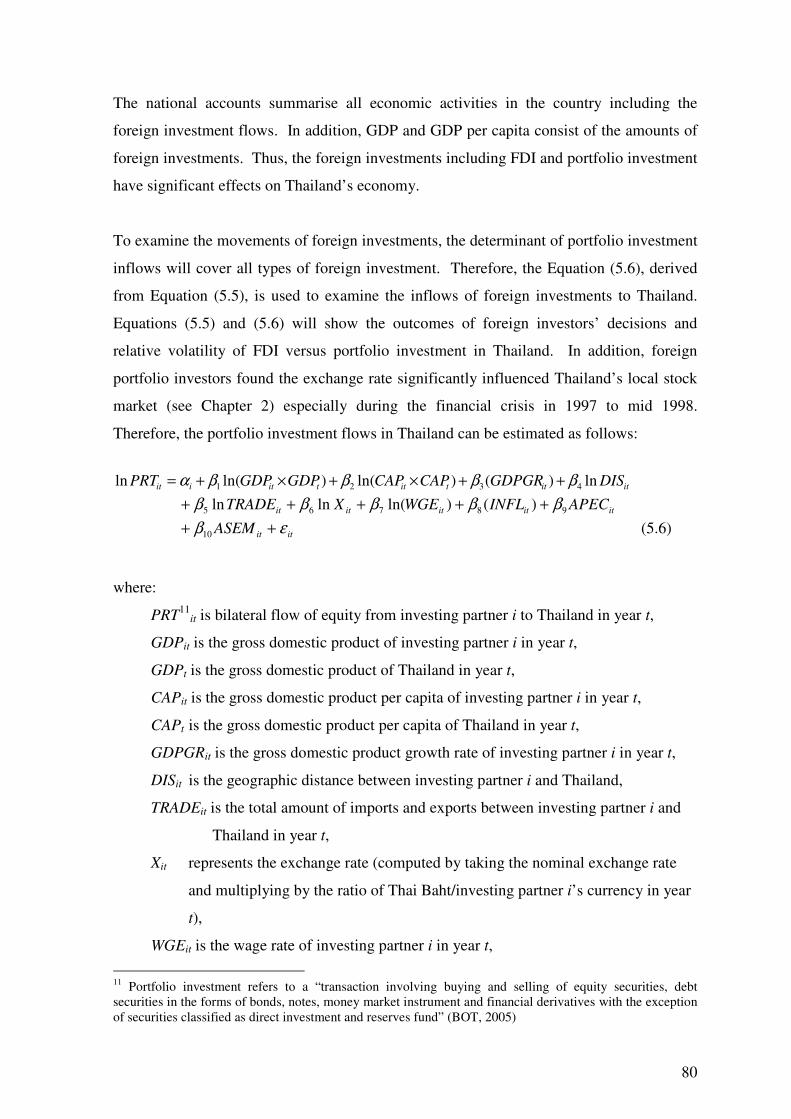
80
The national accounts summarise all economic activities in the country including the
foreign investment flows. In addition, GDP and GDP per capita consist of the amounts of
foreign investments. Thus, the foreign investments including FDI and portfolio investment
have significant effects on Thailand’s economy.
To examine the movements of foreign investments, the determinant of portfolio investment
inflows will cover all types of foreign investment. Therefore, the Equation (5.6), derived
from Equation (5.5), is used to examine the inflows of foreign investments to Thailand.
Equations (5.5) and (5.6) will show the outcomes of foreign investors’ decisions and
relative volatility of FDI versus portfolio investment in Thailand. In addition, foreign
portfolio investors found the exchange rate significantly influenced Thailand’s local stock
market (see Chapter 2) especially during the financial crisis in 1997 to mid 1998.
Therefore, the portfolio investment flows in Thailand can be estimated as follows:
itittittitiit DISGDPGRCAPCAPGDPGDPPRT ln)()ln()ln(ln 4321 ββββα ++×+×+=
ititititit APECINFLWGEXTRADE 98765 )()ln(lnln βββββ +++++
ititASEM εβ ++ 10 (5.6)
where:
PRT11
it is bilateral flow of equity from investing partner i to Thailand in year t,
GDPit is the gross domestic product of investing partner i in year t,
GDPt is the gross domestic product of Thailand in year t,
CAPit is the gross domestic product per capita of investing partner i in year t,
CAPt is the gross domestic product per capita of Thailand in year t,
GDPGRit is the gross domestic product growth rate of investing partner i in year t,
DISit is the geographic distance between investing partner i and Thailand,
TRADEit is the total amount of imports and exports between investing partner i and
Thailand in year t,
Xit represents the exchange rate (computed by taking the nominal exchange rate
and multiplying by the ratio of Thai Baht/investing partner i’s currency in year
t),
WGEit is the wage rate of investing partner i in year t,
11 Portfolio investment refers to a “transaction involving buying and selling of equity securities, debt securities in the forms of bonds, notes, money market instrument and financial derivatives with the exception of securities classified as direct investment and reserves fund” (BOT, 2005)
81
INFLit is inflation rate of investing partner i in year t,
APECit and ASEMit are dummy variables (to capture the regional effects) of investing
partner i and Thailand in year t, and
itε is an error term.
Equation (5.5) is the extended Gravity Model of FDI inflow to Thailand and Equation (5.6)
is the extended Gravity Model of portfolio investment in Thailand for both one-way and
two-way error component models. Individual effects (α) are included in the regressions to
test whether they are fixed or random using the Breusch-Pagan’s Lagrange multiplier test
and Hausman specification test (Baltagi, 2005; Bangnai and Manzocchi, 1999; Stock and
Watson, 2003). In order to find the best approximation of the extended Gravity Model, the
Hausman test is used to test whether the random effects model is more efficient than the
fixed effects model.
This study uses panel data from 1980 to 2004. Thus, the general structure of the panel data
model can be written as follows (Baltagi, 2005; Kang, 2003):
ititit XY εβα +′+= (5.7)
The data set consists of multiple observations. The subscript t = 1, .., T indicates time
series observations and the subscript i = 1, ..., N indicates cross-sectional observations
units such as households, individuals, firms, countries, etc. (Baltagi, 2005). The term α is
the intercept coefficient, β is the slope of the coefficients to be estimated, Xit represents the
explanatory variables, and itε is an error term, assuming E ( itε ) = 0 and Var ( itε ) = 2
εσ .
The variations across individual countries or the time effect of this structure can be
analyzed with a simple shift of regression function, including both one-way error
component and two-way error component models for fixed and random effects models,
respectively. Sections 5.2.3 and 5.2.4 discuss the important feature of these two models in
details with certain assumptions on country and time specific effects in panel data analysis.
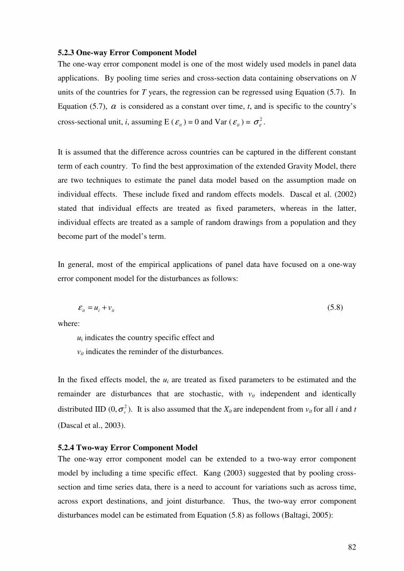
82
5.2.3 One-way Error Component Model
The one-way error component model is one of the most widely used models in panel data
applications. By pooling time series and cross-section data containing observations on N
units of the countries for T years, the regression can be regressed using Equation (5.7). In
Equation (5.7), α is considered as a constant over time, t, and is specific to the country’s
cross-sectional unit, i, assuming E ( itε ) = 0 and Var ( itε ) = 2
εσ .
It is assumed that the difference across countries can be captured in the different constant
term of each country. To find the best approximation of the extended Gravity Model, there
are two techniques to estimate the panel data model based on the assumption made on
individual effects. These include fixed and random effects models. Dascal et al. (2002)
stated that individual effects are treated as fixed parameters, whereas in the latter,
individual effects are treated as a sample of random drawings from a population and they
become part of the model’s term.
In general, most of the empirical applications of panel data have focused on a one-way
error component model for the disturbances as follows:
itiit vu +=ε (5.8)
where:
ui indicates the country specific effect and
vit indicates the reminder of the disturbances.
In the fixed effects model, the ui are treated as fixed parameters to be estimated and the
remainder are disturbances that are stochastic, with vit independent and identically
distributed IID (0, 2
vσ ). It is also assumed that the Xit are independent from vit for all i and t
(Dascal et al., 2003).
5.2.4 Two-way Error Component Model
The one-way error component model can be extended to a two-way error component
model by including a time specific effect. Kang (2003) suggested that by pooling cross-
section and time series data, there is a need to account for variations such as across time,
across export destinations, and joint disturbance. Thus, the two-way error component
disturbances model can be estimated from Equation (5.8) as follows (Baltagi, 2005):
83
ittiit vu ++= λε (5.9)
The decomposed error term approach permits the application of the two-way effects model
with respect to country and time specific effects. The term ui denotes a country specific
effect, tλ denotes a time specific effect, and vit is a remainder stochastic disturbance term.
An error structure leads to the use of a two-way error component model (Kang, 2003). In
the two-way error component model, it is assumed that both the country’s specific errors
and time errors are normally distributed random effects.
The panel data estimator also permits two-way fixed effects and random effects models
following similar reasoning to the one-way model. Therefore, Equation (5.9) can be
extended to a more sophisticated model by allowing a time specific component in addition
to a country specific component.
A panel data set offers advantages over cross-section or time series data sets. The benefits
of using panel data analysis include: (1) if the number of observations is very large, it gives
more reliable parameter estimates than the cross-section or time series data sets; and (2) a
panel data set diminishes the multicollinearity problem and the bias of estimation in
regression. Moreover, the use of panel data methodology captures the relevant
relationships among variables over time and is able to examine possible individual effects
(Kang, 2003). In a panel data framework, the model needs to be identified in terms of
country specific effects for each country and time specific effects for a particular year from
the estimation. Therefore, in order to identify factors affecting the FDI inflow and
portfolio investment in Thailand, it is necessary to specify the extended Gravity Model
with time specific effects over a time period for both the one-way and two-way effects
model.
Multiple regression techniques via the LIMDEP and EVIEW can be used to estimate
Equations (5.5) and (5.6). Since individual effects ( ijα ) are included in Equations (5.5)
and (5.6), it is appropriate to choose whether they are to be treated as fixed or as random
by using the Breusch-Pagan’s Lagrange multiplier test and/or Hausman test specification.
84
5.3 Model Specification
According to the literature discussed in Chapters 3 and 4, bilateral FDI and portfolio
investment models in Thailand are functions of GDP, GDP Per Capita, GDP Growth Rate,
Distance, Trade, Exchange Rate, Wage Rate, Inflation Rate, and Regional Integration
(Equation (5.4)). By rearranging and taking a natural logarithm, Equation (5.4) becomes
Equation (5.5) for the FDI model and Equation (5.6) for portfolio investment model.
These variables are factors that influence the level of FDI and portfolio investment in
Thailand. This research categorises these factors into seven groups. They include: market
size (GDP, GDP Per Capita, and GDP Growth Rate); Geographical Distance; Trade;
Exchange Rate; Wage Rate; Inflation Rate; and Regional Integrations (ASEM and APEC).
The hypothesised signs of the variable specify the potential role of the Thai economy in
attracting foreign investors inward in the FDI Equation (5.5) and the portfolio investment
Equation (5.6). In this study, the host country is Thailand and 21 major investing partners
examined including Hong Kong (China and Hong Kong are considered one investing
partner). These 21 major partners invested substantially in Thailand (see Chapter 2). The
seven groups of variables are discussed below.
5.3.1 Market Size
The possible correlation between the market size of a host country or region and the
volume of inward investment is taken into account in most FDI empirical studies
(Anderson, 1979; Buch et al., 2003; Dunning, 1980; Kim, 2000). For example, Kim
(2000) employed GDP as the proxy of market size to represent the location or
internalisation advantage of the host countries (Japan and the US). The author found that
GDP was significant to the determinants of FDI in the host countries. The market size also
represents the location specific advantage of the host country. Moreover, market size and
the national income level are important to consider for the host country, especially for
market-seeking FDI (Guerin, 2006; UN, 1998). The significantly increased coefficient for
GDP represents the patterns of overall distribution of FDI, which is market-seeking rather
than resource-seeking.
Market size and its potential are expected to be strongly significant for the inflow of
foreign investment to Thailand. Chandprapalert (2000) provided evidence that GNP as
85
proxies for the market size and potential is a big attraction for FDI into Thailand. In this
study, the potential role of the market size of Thailand is investigated using three different
measurements: GDP, GDP Per Capita, and GDP Growth Rate.
5.3.1.1 Gross Domestic Product (GDP)
According to the extended Gravity Model, GDP is incorporated into the model as an
explanation of the economic size of countries in many studies (see Martinez-Zarzoso,
2003; Martinez-Zarzoso and Nowak-Lehmann, 2004; Pelletiere and Reinert, 2004).
Pelletiere and Reinert (2004) found a high level of income in the host country indicates a
high level of production, which increases the availability of investment. In contrast,
Martinez-Zarzoso (2003) and Martinez-Zarzoso and Nowak-Lehmann (2004) discovered a
high level of income in home countries suggested a higher amount of source of funds to
invest overseas.
GDP, GDP per capita, or the GDP growth rate is the national income indicator of the size
of economies, which is related to total of production, consumption, and distribution of
goods and services of a country, as identified by Gopinath and Echeverria (2004). GDP is
included in Equations (5.5), (5.6), (5.7), and (5.8) as a proxy to scale bilateral
FDI/portfolio stocks and the level of integration between Thailand and investing partners.
GDP represents total income in investing partners and Thailand. GDP also measures the
level of the country’s economic development and domestic market opportunities for
investors. Moreover, Thailand’s GDP levels reflect the purchasing power and its market
capability. In the long term, a strong and stable GDP will secure FDI and attract new
investors to Thailand.
This research hypothesised a positive relationship between FDI flows and national incomes
of Thailand as well as the investing partners. The relationship between investing partners’
GDPs and Thailand’s GDP captures the levels of market potential from large markets to
Thailand. Therefore, the expected sign of GDP of investing partners and Thailand is
positive. Consequently, it is expected to have a positive impact on the FDI inflows and
portfolio investment into Thailand. Moreover, the GDP affects FDI positively if trade and
FDI are complementary. The theoretical literature suggests that both FDI and trade can be
complementary or supplementary to each other depending on the nature of investment and
Thailand’s characteristics. This study includes the level of economic activity such as GDP,
GDP Per Capita, and GDP Growth Rate into the models. Therefore, a positive relationship
86
is expected, the larger the economic size of Thailand, the more likely that Thailand
receives foreign investment.
5.3.1.2 Gross Domestic Product Per Capita (GDP Per Capita)
The GDP per capita income is defined as a proxy for the country K/L (capital/labour) ratio.
Many studies ignored per capita incomes, but Bergstrand (1989) argued the per capita
income is appropriate with the Gravity Model. Bergstrand applied GDP per capita as a
proxy of the country’s capital-labour endowment ratio and suggested that if GDP per
capita is significant and negative, it could imply the country has labour intensive
production. In terms of consumption, Bergstrand also concluded that if GDP per capita is
significant and positive, a country has luxurious consumption.
The expected sign of GDP per capita may be positive or negative depending on the
strategic factors driving FDI (a capital or labour intensive industry). According to Buch et
al. (2003) and Limao and Venables (2001), if FDI attracts the Thai domestic service
market, GDP per capita should be positive since it would signal a higher purchasing power
in Thailand. On the other hand, if FDI is encouraged to produce and to export to other
countries, GDP per capita should have a negative sign since it implies relatively low labour
costs in Thailand. Hence, GDP per capita may increase trade relative to FDI-based
production.
It is possible to aggregate the GDP Per Capita in this study. Note GDP Per Capita is
included in equations (5.5), (5.6), (5.10), and (5.11) because the GDP Per Capita is a
positive measurement, implying that larger values indicate greater quality and relationship
between the 21 investing partners and Thailand. GDP Per Capita has also been very
commonly employed in the Gravity Model (see Dascal et al., 2002) and it takes into
account the idea that as income increases, the effect of foreign investment in Thailand may
increase. In Thailand, GDP per capita has an impact on the volume of bilateral FDI and
the portfolio investment. Thus, the expected sign of GDP per capita coefficient can be
positive or negative depending on the Thai government’s strategy on investment policy.
5.3.1.3 Gross Domestic Product Growth Rate
The GDP Growth Rate specified in Equations (5.5) and (5.6) is defined as a return of
investing partners’ equity markets or the rate of return to FDI. The GDP growth rate can
87
be characterised as FDI-led and it is often used as proxies for the size and growth of
market demand and supply.
A selection algorithm to reduce multicollinearity, the possible problems of endogenous and
multicollinearity of GDP growth rate and FDI/Portfolio models are carefully dealt with in
using panel data. These equations identify the GDP Growth Rate in investing partners
which affects the investment in Thailand. FDI/portfolio investment will be moved to
Thailand with a stable and high level of GDP growth rate from the investing partners to
Thailand. Thus, the expected sign for GDP Growth Rate should be positive.
5.3.2 Geographical Distance
According to Bergstrand (1985, 1989) and Portes and Rey (2005), experiments verified
that distances between capital cities and financial centres showed similar results.
Therefore, the geographical Distance in this study represents the navigable distance
between the capital of Thailand, Bangkok, and the capital cities of investing partners.
Distance serves as a proxy for all possible transportation, public infrastructure, and
operating costs such as placing personnel abroad, costs of local tax laws and regulations,
language and cultural differences, communication costs, and costs of being outside
domestic networks (see Bougheas et al., 1999; Brenton et al., 1999; Limao and Venable,
2001). Bougheas et al. (1999) stated that distance inhibited transaction flow by increased
transportation and other transactions costs. Therefore, distance can have direct and indirect
effects on the investment climate between Thailand and investing partners. Distance can
potentially act as a barrier to interaction among economic institutions via tax laws and
regulations. Moreover, distance also affects the investment equations since the costs of
operating overseas are likely to rise the further from the main headquarters or their home
countries (Brenton et al., 1999). Portes and Rey (2005) suggested that distance is the most
important determinant of transaction flows in foreign investment. Guerin (2006) presented
distance as a proxy for information costs, rather than transport costs, in the FDI and equity
flows. The cost of information gathering would likely increase with distance, as
familiarity with the host country’s investment opportunities, customs, and culture
decreases.
In the Gravity Model, geographical Distance is generally included as an explanatory
variable (Portes and Rey, 2005; Stone and Jeon, 1999). Geographical distance may cause
88
countries to change from exports (trade) to invest overseas in order to reduce transportation
and production costs (Gopinath and Echeverria, 2004). This implies investing partners
may be encouraged to invest directly in Thailand for the purpose of reducing transportation
costs, information costs or to serve the customers better. Thus countries with large
domestic markets, or close to larger markets, may be more attractive to investors than
smaller or more remote markets. Furthermore, the more open a country with advances in
transportation densities and short distances from markets can attract investors even if it is
surrounded by smaller markets. Further, investments in infrastructure can reduce gaps
between the capital cities, financial centres, and small towns in the countryside (IMF,
2004).
Therefore, the Distance coefficient in Equations (5.5) and (5.6) is expected to be negative
since it is a proxy of all possible investment barriers which inhibit foreign investment by
distance. It implies that increases in these investment costs will have a negative effect on
FDI/portfolio investment flows into Thailand.
5.3.3 Trade
Equations (5.5) and (5.6) include bilateral Trade as an independent variable to examine
whether trade complements FDI activity (when the coefficient of Trade is significantly
positive) or supplements FDI activity (when the coefficient of Trade is significantly
negative) following the Stone and Jeon (1999) approach. Trade is designed to indicate the
openness of the Thai economy which is similar to Bevan and Estrin (2004) and Ismail and
Yussof’s (2003) study. Consequently, the higher the level of openness of the Thai
economy, the easier it is for investors to invest in and trade with Thailand.
It is more appropriate to refer to the distinction between horizontal and vertical FDI, since
it can explain more about the complementary or supplementary relationship between FDI
and trade for investing partners and Thailand. If the main motivation of foreign investors
is to produce for the Thai market or to export to other countries in the same region, that
would be horizontal FDI, otherwise it would be vertical FDI.
Trade has lower risk but higher liquidity problems compared with FDI, but Guerin (2006)
argued that the developed countries (such as US, Japan, and UK which are the major FDI
in Thailand) may prefer FDI to trade when access to larger markets is the key motivation.
89
Trade is highly sensitive to changes in market size in Thailand. For example, if there is a
negative output shock, trade flows will be more impulsive than FDI. Furthermore, distance
can reduce the trade flow but increase the investment because the investing country would
like to reduce transport costs by investing in manufacturing in Thailand (see Bergstrand,
1985).
The openness of the Thai economy is expected to attract FDI inflows. Hence, the Trade
coefficients in Equations (5.5) and (5.6) are expected to be positive. In this study, Trade
refers to total imports and exports from Thailand to an investing partner i in year t.
However, Thailand may prefer FDI to trade because FDI would improve Thailand’s
development interests such as technology development, the level of infrastructure, as well
as the level of openness of the economy.
5.3.4 Exchange Rate
Exchange rate is included in Equations (5.5) and (5.6) as one of the most essential
components affecting FDI. Exchange rate volatility may affect direct investment and
portfolio investment negatively. A volatile exchange rate might reduce investment. It was
first introduced in the Gravity Model by Berstrand (1985; 1989). Exchange rate
movements are relevant and significant to FDI in spite of exchange rate volatility because
exchange rate volatility directly contributes to uncertainty on the returning transaction plan
from the investing countries (see Guerin, 2006; Hubert and Pain, 2002; Rose, 2000).
The exchange rate affects the relative currency prices of closely matched manufactured
goods produced in different countries. In terms of trade, an increase in the value of an
importing country’s currency implies a depreciation of the Thai Baht and is expected to
have a positive impact on exporting products that are produced in Thailand. A higher
value investing partner currency enables investors to invest in the Thai economy more
inexpensively, thus the amount of FDI will rise. A higher value currency from an
investing partner also makes exporting products more expensive to Thai purchasers, so
again FDI in Thailand would be stimulated to overcome this cost disadvantage (Grosse and
Trevino, 1996; Isard, 1977).
The Bank of Thailand (BOT) controls the current foreign exchange in maintaining
exchange rate stability (Julian, 2001). During the 1997 Asian Financial Crisis, the Thai
90
government floated the Thai Baht, triggering a collapse of the financial sector resulting in
economic recession. The value of the Thai Baht fell from 25 to the US Dollar to 40 in
2004 (BOT, 2004). The Thai Baht was attacked by foreign speculators and the Thai
government failed to defend its currency. Moreover, the finance and real estate categories
were weak before the crisis. The value of Thai Baht dropped rapidly to the lowest point of
56 Baht per US Dollar in January 1998. By the fourth quarter of 2004, the Thai Baht
almost reached its previous high of 40 Baht per US Dollar. The coefficient of Exchange
Rate is expected to be positive because most investors take advantage of the depreciation
of the Thai Baht (Equations (5.5) and (5.6)) to reduce their costs of investment (see Bajo-
Rubio and Sosvilla-Rivero, 1994; Blonigen, 1997; Froot and Stein, 1991).
5.3.5 Wage Rate
According to neo-classical theories, wage rate is considered in the cost minimisation
strategies of firms. Wage rate differentials were considered as an important determinant of
FDI (see Bevan and Estrin, 2004; Ismail and Yussof, 2003; Milner et al., 2004). Dunning
(1980) argued that real wage cost is more likely to influence the model of servicing in
developing country markets than in developed country markets. Bevan and Estrin’s (2004)
study used labour cost in the host country to evaluate alternative locations based on a real
cost to ensure that a lower wage was not compensated by reduced labour productivity or by
an overvalued currency. Their findings showed labour costs are negative and significant to
FDI, which supports their hypothesis that foreign investors are cost sensitive. In contrast,
Milner et al. (2004) used the labour cost from the home country (Japan) to consider
shifting investment to Thailand. The results indicated that labour cost affects the
magnitude of FDI and the greater the labour intensity in Japan, the greater the amount of
the corresponding (magnitude of) FDI in Thailand.
Roberto (2004) argued that when foreign investors decide to build new production
facilities overseas, they are strongly influenced by location decision of previous ‘foreign’
investors and the labour costs and availability of labour.
Wage rate is included in Equations (5.5) and (5.6) to capture the intensity and costs of
labour in production of the investing partners. Evaluating the relative impact on the
investing partners, the low wage of local labour decreases the expansion of overseas
investment. The higher level of wage rate in their countries stimulates FDI outflows to
91
substitute for lower labour cost of production. Thus, the coefficients of Wage Rate are
expected to be positive because investors evaluate alternative production locations in
Thailand to ensure that there will be a lower wage rate than in their countries.
5.3.6 Inflation Rate
Inflation rate is considered a proxy for the quality of macroeconomic management. The
inflation rate is measured by the changes in the consumer price index which is a weighted
average of price of goods and services consumed. A high inflation rate indicates high
economic tension in a country, and reflects the inability or unwillingness of the
government to conduct a stable economic policy. It can be argued that if foreign investors
are risk-averse (or even risk-neutral), a higher inflation rate may lead to a reduction in FDI
in the host country, because investors will not risk profits expected from investment. As
long as there is uncertainty, foreign investors will demand a high price to cover their
exposure to inflation risks, and this, in turn, will decrease the volume of investment. Thus,
to encourage investment, the stability of the inflation rate is important.
Inflation Rate, as measured by consumer price indexes from the investing partners, is
included in Equations (5.5) and (5.6). Foreign investors who transfer profits to their
countries would benefit if the inflation rate in their countries is high since the currency
would have more value when converted to domestic currencies. In this case, foreign
investors’ profits are higher as a result of the appreciated exchange rates.
Thus, the expected sign for Inflation Rate of the investing partners will be positive which
implies an increase of the average price level and the purchasing power in investing
country’s economies.
5.3.7 Regional Integrations
Regional integrations are political or semi-economic in nature and governments which
pursue integration hope to decrease barriers among members and political uncertainty.
Regional integrations evaluate the effect of preferential investment agreements among
member nations and indicate the consolidation and effectiveness among the group
members. The FDI policies, as well as their perceived feedback, influence attitudes toward
negotiating a multilateral framework for investment. Head et al. (1999) demonstrated that
countries which offered industrial estates, job-creation subsidies, and low taxes received
significantly higher foreign investment.
92
The coefficients for all regional integrations are expected to be positive, since they affect
the FDI inflow and the operation of the capital market in Thailand. This could imply that
APEC and ASEM stimulated the FDI between Thailand and these member countries.
APEC and ASEM are included in the models to represent the close relationship between
investing partners and Thailand. These regional integrations measure Thai security
interests from investing partners and the degree of political alliance or friendliness between
the parties involved. Consequently, investing partners might want to join a regional
integration association such as ASEM and APEC to take higher benefits. By joining
APEC and ASEM, investing partners have better opportunities to establish contacts with
Thai businesses and further increase their investment relationship with Thailand. Thailand
is considered as the gateway to other neighbouring countries’ markets as the hub of the
“golden pentagon” comprising Myanmar and Indo-China, which has a potential market
size of more than 145 million consumers. Many foreign countries may decide to locate
their manufacturers in Thailand to take advantage of this market (UNCTAD, 2004). The
market potential is significant for economic integration which has a direct effect on
internationalisation by reducing transaction and information costs (see Chandprapalert,
2000; Guerin, 2006; Martinez-Zarzoso, 2003).
Equations (5.5) and (5.6) suggest that bilateral FDI and portfolio investment depend on
each country’s market size, Distance, Trade, Exchange Rate, Wage Rate, Inflation Rate,
and Regional Integrations. Table 5-2 summarises the expected signs of the parameter
estimates on the explanatory variables used in modelling the Gravity model equations. A
positive sign (+) indicates an anticipated positive effect on FDI/portfolio investment. A
negative sign (-) indicates an anticipated negative effect on FDI/portfolio investment.
Table 5-2 shows the hypothesised signs of the variable on FDI models and portfolio
investment models. For example, Trade is hypothesised to be positively related to the FDI
and portfolio investment.

93
Table 5-2: Variables Descriptions and Expected Signs
Variable
Description Expected Sign
GDP Gross domestic product in investing partner i and Thailand
+, +
GDP Per Capita Gross domestic product per capita in investing partner i and Thailand
+/-, +/-
GDP Growth Rate Gross domestic product growth rate in investing partner i +, +
Distance The geographical distance between the capital cities of investing partner i and Bangkok, Thailand
-, -
Trade Total imports and exports between Thailand and investing partner i
+, +
Exchange Rate Value of bilateral exchange rate Thai Baht per 1 investing partner i’s currency
+, +
Wage Rate A basic wage per hour in US Dollar of investing partner i
+, +
Inflation Rate Percentage at the consumer price in investing partner i +, +
Regional Integration
Value equal to “1” if investing partner i and j are members of each specific regional grouping such as ASEM, APEC in year t, and “0” otherwise
+, +
5.4 Data Source
This study examines a number of countries involved in FDI activity in Thailand. The data
set is limited by the amount of information available for each country involved. Equations
(5.5) and (5.6) cover the period from 1980 to 2004. The data are obtained from the “UN’s
World Investment Directory”, “OECD’s Foreign Direct Investment Statistics Yearbook”,
and “Central Intelligence Agency World Factbook”, the World Resources Institute. Other
data sources from Thai organizations include the Board of Investment (BOI), National
Economic and Social Development Board (NESDB), and Bank of Thailand (BOT).
Additional data are collected from the “IMF’s International Financial Statistics or IMF’s
Direction of Trade Statistics Yearbook”. Distances between cities are obtained from the
website (www.indo.com/distance). Investing partners with more than 90% of total FDI
inflows and portfolio investment to Thailand (Table 2-4, and Appendix A) are chosen. The
data set consisted of 35 countries including India, New Zealand, Spain, Portugal, Brunei
Darussaram, Taiwan, Ireland, Laos, Myanmar, Cambodia, and Vietnam. However, many
countries have missing data on many variables due to the low quality of the database
system, political policy, and low degree of openness. These countries are excluded in the
empirical analysis because their total FDI inflows into Thailand are less than 5% (see
94
Table 2-4). The summary of data sources and descriptive statistics for the variables are
presented in Appendix B.
Finally, the empirical analysis is divided into 21 groups of investing partners (22
economies) following the BOI criteria: Japan, US, Austria, Belgium, Germany, Denmark,
Finland, France, UK, Italy, Netherlands, Sweden, Indonesia, Malaysia, Philippines,
Singapore, South Korea, China and Hong Kong, Canada, Australia, and Switzerland. The
FDI manufacturing is separated into nine categories following the BOI and BOT
framework: (1) agricultural products; (2) mining and quarrying; (3) industry; (4) financial
institutions; (5) trade; (6) services; (7) investment; (8) real estate; and (9) others (BOI,
2005; BOT, 2004).
5.5 The Effects of the 1997 Asian Financial Crisis on FDI and Equity Flows to Thailand
Before 1997, relatively low yields in industrial countries, and impressive economic growth
and attractive returns in developing countries have motivated investors from industrial
countries to invest their funds in the East. Thailand was one of the countries which
benefited from this growth. For example, Thailand received capital inflows from Japan in
the form of FDI and exports, as a result of Yen appreciation (Siamwalla et al., 1999;
Tiwari et al., 2003). The Thai government decided to remove its exchange controls in
1991 to liberalise financial institutions, but left the fixed exchange rate unchanged.
Consequently, Thailand’s net capital inflow doubled from US$ 6 billion in 1990 to US$ 11
billion in 1996 (see Table 2-2). There was a big increase in portfolio inflows from US$ 2.7
billion per annum in 1990-1992 to US$ 7 billion per annum in 1993-1996. The influx led
to the booming of the stock market index, P/E ratio, and market capitalisation that strongly
attracts foreign investors, especially in 1995. From 1990 to 1996, Thailand experienced
sustainable economic growth with an annual average growth rate of 8% per annum (see
Table 2-1).
However, the market began to question Thailand’s microeconomic and macroeconomic
stability and the capability of the government to sustain the stability of financial system.
This led to both creditors and investors rapidly withdrawing their funds, which coincided
with debt repayments. The resulting capital outflows forced the Thai government to float
95
the Baht exchange rate in July 1997, sparking a series of financial crises in East Asia and
other regions.
Thailand floated the Baht on 2 July 1997. Thailand was essentially bankrupt and the Bank
of Thailand made huge numbers of forward commitments to sell foreign currency in order
to defend the Baht against speculators (Sussangkarn, 1999). Consequently, net
international reserves fell to US$ 27 billion by the end of 1997 (see Table 2-1).
After the float, net capital outflows peaked in the third quarter of 1997 and the Baht kept
depreciating. The exchange rate stayed above 40 Baht per US Dollar throughout the fourth
quarter of 2004. The effects of the financial crisis on Thailand’s economy were severe.
The GDP growth rate of Thailand declined from 7.7% in 1996 to -2.68% in 1998 (NESDB,
2004). Interest rates during the crisis in Thailand increased from 13% to 15% and the
currency depreciated against the US Dollar to 56 Baht per US Dollar in January 1998. In
addition, the ordinaries index of SET (Stock Exchange of Thailand) fell by over 75%
(SET, 2004). Furthermore, the social impacts of the crisis were quite severe in Thailand.
For example, the level of poverty increased during this period due to inflation (up to 8%),
and the number of unemployed in February 1998 was 1.1 million more than in 1997 (0.94
million). The number of underemployed (who work less than 20 hours a week) was 0.8
million, out of a total labour force of 30 million (Siamwalla et al., 1999).
The 1997 Asian Financial Crisis caused structural changes in the determinants of FDI and
portfolio investment in Thai economy. To test the changes from the 1997 Asian Financial
Crisis, this study defines two different time periods: first is the pre-crisis period and second
is the post-crisis period.
To study the effects of the 1997 Asian Financial Crisis on the FDI and portfolio investment
in Thailand (integrating the pre- and post-crises), it is important to test the linear
relationships to find whether the coefficients changed over the sample period 1980 to 2004
(Greene, 2003). Equations (5.5) and (5.6) will be used to test for the structural changes
using dummy variables suggested by Perron (1989).
Let τ denote the hypothesized break year and let Dt(τ) be a binary variable that equals zero
before the break year t and after, so Dt(τ) = 0 if t (year) ≤ τ and Dt(τ) = 1 if t > τ. From
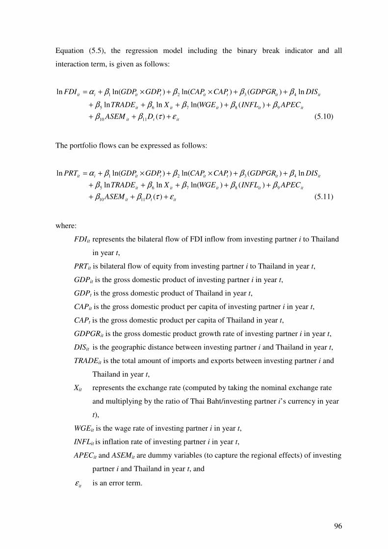
96
Equation (5.5), the regression model including the binary break indicator and all
interaction term, is given as follows:
itittittitiit DISGDPGRCAPCAPGDPGDPFDI ln)()ln()ln(ln 4321 ββββα ++×+×+=
ititititit APECINFLWGEXTRADE 98765 )()ln(lnln βββββ +++++
ittit DASEM ετββ +++ )(1110 (5.10)
The portfolio flows can be expressed as follows:
itittittitiit DISGDPGRCAPCAPGDPGDPPRT ln)()ln()ln(ln 4321 ββββα ++×+×+=
ititititit APECINFLWGEXTRADE 98765 )()ln(lnln βββββ +++++
ittit DASEM ετββ +++ )(1110 (5.11)
where:
FDIit represents the bilateral flow of FDI inflow from investing partner i to Thailand
in year t,
PRTit is bilateral flow of equity from investing partner i to Thailand in year t,
GDPit is the gross domestic product of investing partner i in year t,
GDPt is the gross domestic product of Thailand in year t,
CAPit is the gross domestic product per capita of investing partner i in year t,
CAPt is the gross domestic product per capita of Thailand in year t,
GDPGRit is the gross domestic product growth rate of investing partner i in year t,
DISit is the geographic distance between investing partner i and Thailand in year t,
TRADEit is the total amount of imports and exports between investing partner i and
Thailand in year t,
Xit represents the exchange rate (computed by taking the nominal exchange rate
and multiplying by the ratio of Thai Baht/investing partner i’s currency in year
t),
WGEit is the wage rate of investing partner i in year t,
INFLit is inflation rate of investing partner i in year t,
APECit and ASEMit are dummy variables (to capture the regional effects) of investing
partner i and Thailand in year t, and
itε is an error term.
97
If there is no break in equations (5.10) and (5.11), then 11β is insignificant.
5.6 The Relationship between FDI and Industrial Categories across Thailand
This study also investigates the relationship between FDI and industrial categories across
Thailand during the period 1980-2004. There are nine industrial categories following the
BOI and BOT framework: agricultural products, mining and quarrying, industry, financial
institutions, trade, services, investment, real estate, and others (BOI, 2005; BOT, 2004).
Using the country-level data available in the inflows of FDI, the regressions are estimated
for all nine industrial categories to determine the influences of FDI in the industrial
categories in Thailand.
To estimate the relationship between FDI inflows and the nine industrial categories
(industry, financial institutions, trade, mining and quarrying, agricultural products,
services, investment, real estate, and others), the seemingly unrelated regression estimation
(SURE) was employed. Zellner (1962) stated that the SURE model can be applied to
analyse data when regressions for several commodities are to be estimated. SURE is a
technique for analysing a system of multiple equations with cross-equation parameter
restrictions and correlated error terms (Greene, 2003). SURE may contain multiple
equations which are independent with different independent variables. SURE allows
correlated errors between equations. SURE developed prior information on the
disturbance variances that reduce the number of parameters in the disturbance covariance
matrix.
To estimate SURE (Greene, 2003; Kontoghiorghes, 2000; Zellner, 1962):
yi = Xiβi + ui, i = 1, …., G (5.12)
where:
yi is the response vectors,
Xi is the exogenous matrix with full column ranks,
βi is the coefficients,
ui is the disturbance term, with E(µi,) = 0 and E(µi µjT) = σijIT(i, j = 1, ….., G), and
G is the number of equations.
98
Assume each equation has k observations. Then the reduced form of the SURE model
computing the GLS estimation for βi can be written as follows:
( ) iiiii YVXXVX111ˆ −−− ′′=β (5.13)
where:
EC(Y) = ( )1
i
G
iX
=⊕ VEC({ } )() UVECGi +β (5.14)
where:
Y = (y1….yG) and U = (u1…uG). Let ∑ be a G×G matrix i
G
i X1=⊕ defines the G×K
block-diagonal matrix:
X1
i
G
iX
1=⊕ = nXXX ⊕⊕⊕ ...21 = X2 (5.15)
……
XG
where:
K = ∑ = i
G
i k1
The set of matrices used in the direct sum are not necessarily of the same dimension
(Kontoghiorghes, 2000).
The SURE strategy can be applied to co-integrating regressions to obtain asymptotically
efficient estimators when the equilibrium errors are correlated across equations. Moreover,
Mark et al. (2005) suggested that SURE is applicable for panel co-integration estimation in
environments where the cross-section is small relative to the available time series.
Therefore, a test of regression coefficient vectors is applied in the analysis.
This study analyses the role of FDI in Thailand across industry sectors and uses 25 years of
time series data, from 1980 to 2004. Thus, to examine the relationship between FDI in
each industrial category, Equation (5.16) examines the routinely calculated variance
inequalities and correlations constraints as follows:
FDIk = β1 + β2GDPkt + β3Kkt + β4IFLt + β5X_USt + β6RESt + β7CURt + β8NNSVt
+ β9WGEt + β10UNEMt + β11ASEMt + β12APECt + u (5.16)
99
where:
FDIk is the FDI in each k industrial category: industry, financial institutions, trade,
mining and quarrying, agricultural products, services, investment, real estate,
and others, in year t,
GDPk is the GDP in k industrial categories in year t,
Kk is the net capital stock in k industrial categories in year t,
IFL is the inflation rate in year t,
X_US is the exchange rate (Thai Baht per US Dollar) in year t,
RES is the international reserves in year t,
CUR is the total current account balance in year t,
NNSV is the total national saving in year t,
WGE is the minimum wage rate per day in Thailand in year t,
UNE is the unemployment rate in Thailand in year t,
ASEM, APEC are dummy variables (to capture the regional effects) that equal 1 if
Thailand becomes a member of either ASEM or APEC in year t, and “0”
otherwise in year t.
The summary of data sources and the descriptive statistics for the variables are presented in
Section 5.3 and Appendix B.
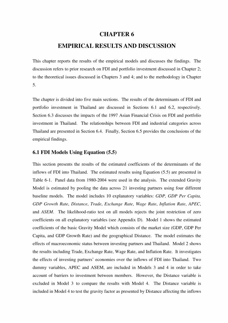
CHAPTER 6
EMPIRICAL RESULTS AND DISCUSSION
This chapter reports the results of the empirical models and discusses the findings. The
discussion refers to prior research on FDI and portfolio investment discussed in Chapter 2;
to the theoretical issues discussed in Chapters 3 and 4; and to the methodology in Chapter
5.
The chapter is divided into five main sections. The results of the determinants of FDI and
portfolio investment in Thailand are discussed in Sections 6.1 and 6.2, respectively.
Section 6.3 discusses the impacts of the 1997 Asian Financial Crisis on FDI and portfolio
investment in Thailand. The relationships between FDI and industrial categories across
Thailand are presented in Section 6.4. Finally, Section 6.5 provides the conclusions of the
empirical findings.
6.1 FDI Models Using Equation (5.5) This section presents the results of the estimated coefficients of the determinants of the
inflows of FDI into Thailand. The estimated results using Equation (5.5) are presented in
Table 6-1. Panel data from 1980-2004 were used in the analysis. The extended Gravity
Model is estimated by pooling the data across 21 investing partners using four different
baseline models. The model includes 10 explanatory variables: GDP, GDP Per Capita,
GDP Growth Rate, Distance, Trade, Exchange Rate, Wage Rate, Inflation Rate, APEC,
and ASEM. The likelihood-ratio test on all models rejects the joint restriction of zero
coefficients on all explanatory variables (see Appendix D). Model 1 shows the estimated
coefficients of the basic Gravity Model which consists of the market size (GDP, GDP Per
Capita, and GDP Growth Rate) and the geographical Distance. The model estimates the
effects of macroeconomic status between investing partners and Thailand. Model 2 shows
the results including Trade, Exchange Rate, Wage Rate, and Inflation Rate. It investigates
the effects of investing partners’ economies over the inflows of FDI into Thailand. Two
dummy variables, APEC and ASEM, are included in Models 3 and 4 in order to take
account of barriers to investment between members. However, the Distance variable is
excluded in Model 3 to compare the results with Model 4. The Distance variable is
included in Model 4 to test the gravity factor as presented by Distance affecting the inflows
101
of FDI into Thailand. Therefore, Model 4 shows the empirical results for all explanatory
variables.
In addition, we also test for stationarity with the Augmented Dickey-Fuller (ADF) test for
all models. The unit root test rejected the null hypotheses for each of the variable. The
result shows the variables are stationary. The FDI models (see Table 6-1) in Thailand are
one-way error component models which are supported by the techniques to estimate panel
data models. The F-test and Breusch-Pagan’s Lagrange multiplier test reject the null
hypothesis of a common intercept (see Chapter 5). When choosing between fixed and
random effects, the Hausman tests fail to accept the null hypothesis (the random effects
model is preferred). The results in Table 6-1 show that the fixed effects models generated
the most reliable results used in this study. All models show that most of the estimated
coefficients have the hypothesised signs and are statistically significant. In addition, the
explanatory powers of all four models (R2) are high, they are between 69%-71%, and the
specification F-statistics are statistically significant at the critical 1% level.
All the variables have the hypothesised signs except Exchange Rate (in Models 2, 3, and
4), Distance (in Models 1, 2, and 4), and APEC (in Models 3 and 4), but Distance and
APEC are insignificant. The Exchange Rate contradicts to hypothesised signs and it is
statistically significant only in Models 3 and 4. The results show the coefficients of GDP,
GDP Per Capita, GDP Growth Rate, Trade, Wage Rate, Inflation Rate, and ASEM
variables are statistically significant with the hypothesised signs in all models. However,
Distance and APEC coefficients are not significantly different from zero at the 10% level
of significance in all models.
GDP is included in estimating Equation (5.5) to capture the effect of the size of economies
between Thailand and the 21 investing partners. GDP is positive and statistically
significant at the 1% level of significance in all models. When the regional integration
variables are included in Models 3 and 4, the coefficient values of GDP are smaller in
Models 3 and 4 than in Models 1 and 2. This suggests that the inflows of FDI into
Thailand are affected by other factors beside GDP. The significant positive sign on GDP
indicates that the FDI flows into Thailand are strongly oriented toward capturing the local
market in Thailand and domestic markets in the investing partners. This finding is
consistent with previous studies (see Nakamura and Oyama, 1998; Portes and Rey, 2005;
102
Table 6-1: Determinants of FDI in Thailand Using Equation (5.5)
Variable Coefficients
Model 1a 2b 3c 4d
GDP 4.6550*** 4.8243*** 4.2077*** 4.2077***
GDP Per Capita -3.8255*** -3.8881*** -3.2523*** -3.2523***
GDP Growth Rate .0164 .0612 .0751** .0751**
Distance .4351 .2538 - .0387
Trade - .0976** .1124** .1124**
Exchange Rate - -.3441 -.4788** -.4788**
Wage Rate - .1176** .1245*** .1245***
Inflation Rate - .0776*** .0869*** .0869***
APEC - - -.3623 -.3623
ASEM - - .6779*** .6779***
No. of observations 525 525 525 525
Mean 2.0851 2.0851 2.0851 2.0851
Std. Dev. 1.7984 1.7621 1.7446 1.7464
Sum of squares 1617.06 1540.07 1506.62 1506.62
R2 69.32% 70.78% 71.41% 71.41%
Adjusted R2 67.84% 69.13% 69.74% 69.68%
F-Statistics 47.06*** 42.90*** 42.64*** 41.13***
Hausman-test 28.13*** 44.05*** 31.37*** 41.55***
FEM FEM FEM FEM
Notes: i. ***, **, and * represent statistical significance at the 1%, 5% and 10% levels, respectively.
ii. FEM is the fixed effects model. iii. 1a Model 1 represents the basic specification of extended Gravity Model which
includes GDP, GDP Per Capita, GDP Growth Rate, and Distance. iv. 2b Model 2 represents the basic specification variables, the macroeconomic
variables of the investing partners (Wage Rate and Inflation Rate) and the economic relationship variables between Thailand and the investing partners (Trade and Exchange Rate).
v. 3c Model 3 includes APEC and ASEM but excludes Distance. vi. 4d Model 4 includes all explanatory variables.
103
Tahir and Larimo, 2005) which confirmed that the GDP of investing partners and Thailand
has a positive effect on FDI. It indicates that a large market size in both investing partners
and Thailand has a significant positive effect on attracting FDI.
Based on results of GDP (Table 6-1), an increase of GDP for both investing partners and
Thailand raises the affiliate activity of FDI in Thailand, this is because the coefficient of
GDP is income-elastic. Thus, a large size of economies in both investing partners and
Thailand increase the FDI in Thailand. One of FDI’s objectives is to have a large market
share and to achieve this objective FDI produces huge quantities to benefit from economies
of scale. Due to this factor, there is huge market potential to attract FDI in Thailand. It
can be argued that investing partners expect to make more profits through mass production
with lower marginal costs of production in Thailand with larger market size to serve their
products.
The coefficients of GDP Per Capita are negative and statistically significant at the 1% level
of significance in all models. Similar to GDP, when the regional integration variables are
included in Models 3 and 4, the coefficient values of GDP Per Capita are slightly smaller
than in Models 1 and 2. Co-linearity may exist among APEC, ASEM, GDP, and GDP Per
Capita in the regressions, while holding the other variables constant (see Appendix D).
However, GDP Per Capita’s elasticities are quite high (3.3-3.8%), thus confirming the
importance of the agglomeration internalities conferred by GDP Per Capita of both
investing partners and Thailand which may be due to the information internalities
concerning the economic environment. GDP Per Capita, as an indicator of potential
market size, may develop the Thai economy relative to FDI production base. Previous
studies found a negative and significant coefficient of GDP Per Capita, for example,
Bergstrand (1989) suggested that GDP per capita is a proxy for the country’s capital-labour
endowment ratio and the negative coefficient for GDP per capita implies a country has
labour-intensive production (in term of production). Based on the estimated coefficients of
GDP Per Capita (see Table 6-1), this means that Thailand is a labour-intensive and,
simultaneously investing partners are capital-intensive in production. This could be due to
other characteristics that make Thailand attractive to investors (such as a relatively stable
economic environment and steady GDP growth rate). Moreover, Dascal et al. (2002)
argued that an increase in foreign investment stimulates production in the host country,
which is exported back to markets in their countries. Hence, this may increase the bilateral
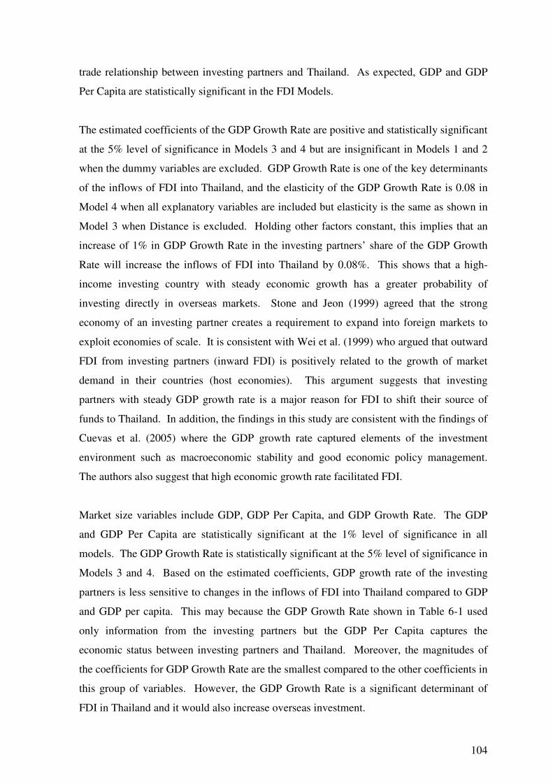
104
trade relationship between investing partners and Thailand. As expected, GDP and GDP
Per Capita are statistically significant in the FDI Models.
The estimated coefficients of the GDP Growth Rate are positive and statistically significant
at the 5% level of significance in Models 3 and 4 but are insignificant in Models 1 and 2
when the dummy variables are excluded. GDP Growth Rate is one of the key determinants
of the inflows of FDI into Thailand, and the elasticity of the GDP Growth Rate is 0.08 in
Model 4 when all explanatory variables are included but elasticity is the same as shown in
Model 3 when Distance is excluded. Holding other factors constant, this implies that an
increase of 1% in GDP Growth Rate in the investing partners’ share of the GDP Growth
Rate will increase the inflows of FDI into Thailand by 0.08%. This shows that a high-
income investing country with steady economic growth has a greater probability of
investing directly in overseas markets. Stone and Jeon (1999) agreed that the strong
economy of an investing partner creates a requirement to expand into foreign markets to
exploit economies of scale. It is consistent with Wei et al. (1999) who argued that outward
FDI from investing partners (inward FDI) is positively related to the growth of market
demand in their countries (host economies). This argument suggests that investing
partners with steady GDP growth rate is a major reason for FDI to shift their source of
funds to Thailand. In addition, the findings in this study are consistent with the findings of
Cuevas et al. (2005) where the GDP growth rate captured elements of the investment
environment such as macroeconomic stability and good economic policy management.
The authors also suggest that high economic growth rate facilitated FDI.
Market size variables include GDP, GDP Per Capita, and GDP Growth Rate. The GDP
and GDP Per Capita are statistically significant at the 1% level of significance in all
models. The GDP Growth Rate is statistically significant at the 5% level of significance in
Models 3 and 4. Based on the estimated coefficients, GDP growth rate of the investing
partners is less sensitive to changes in the inflows of FDI into Thailand compared to GDP
and GDP per capita. This may because the GDP Growth Rate shown in Table 6-1 used
only information from the investing partners but the GDP Per Capita captures the
economic status between investing partners and Thailand. Moreover, the magnitudes of
the coefficients for GDP Growth Rate are the smallest compared to the other coefficients in
this group of variables. However, the GDP Growth Rate is a significant determinant of
FDI in Thailand and it would also increase overseas investment.
105
The coefficients of the Trade variables are positive and statistically significant at the 5%
level of significance in Models 2, 3, and 4. The magnitudes of the coefficients increase
from 0.10 in Model 2 up to 0.11 in Models 3 and 4 when the regional integration variables
are included. That means a 1% increase in Trade will cause FDI to increase by 0.10% in
Model 2 and 0.11% in Models 3 and 4. This implies an increase in Trade is associated
with an increase of the inflows of FDI into Thailand. When Thailand and investing
partners become members of APEC and ASEM, it positively impacts the value of trade
and increases the investment flows into Thailand from overseas.
In order to investigate the plausible impact of FDI on Trade, under the hypothesis of
substitutability following Brenton et al. (1999), the Trade coefficient in Equation (5.5)
should be negative. The results in Table 6-1 suggest that FDI and Trade are
complementary, rather than supplementary. This finding reinforces those of Bevan and
Estrin (2004) and Stone and Jeon (1999) who found a complementary relationship between
FDI and Trade. The positive relationship between Trade and FDI supports the hypothesis
that high levels of trade have a positive effect on the inflows of FDI into Thailand.
For all models (see Table 6-1), GDP, GDP Per Capita, GDP Growth Rate, and Trade are
significant determinants of FDI. Inflows of FDI increases as the GDP, GDP Growth Rate,
and Trade increase. However, the GDP and GDP Per Capita are more sensitive to changes
in FDI compared to Trade. This suggests that economic indicators such as GDP, GDP per
capita, and GDP growth rate, are preferred over the inflows of FDI into Thailand. This
implies that FDI in Thailand is driven more by the income of investing partners than by
Thailand. Ismail and Yussof (2003) and Stone and Jeon (1999) argued that the FDI
activity in Thailand is supply-side driven and represents an important marketing channel
for FDI to export most of their products. This is consistent with the BOI objectives where
the majority of promoted foreign investment in Thailand is export-oriented (BOI, 2005).
However, this result contradicts Guerin’s (2006) findings that showed that trade is more
sensitive and preferred to FDI in the developing counties. In contrast, developed countries
preferred FDI to trade when it is motivated by larger markets.
The estimated coefficients of Exchange Rate are negative and statistically significant at the
5% level of significance in Models 3 and 4 when the dummy variables are included. FDI
is highly sensitive to the exchange rate. This suggests that a depreciation of investing
106
partners’ currencies against the Thai Baht encourages the inflows of FDI into Thailand.
For example, a 1% depreciation of the exchange rate decreases FDI from investing partners
by 0.5% (see Models 3 and 4), other factors being constant. The result contradicts Tahir
and Larimo (2005) who argued that a country can attract FDI by devaluing its currency
because FDI will benefit from currency weakness in the host country. The appreciation of
the Thai Baht actually increases the inflows of FDI into Thailand for three reasons. First,
the investing partners are seeking advantage by exporting new/used production facilities
into Thailand as part of their FDI to Thailand. Thailand is labour-intensive and it lacks
advanced technologies and equipment which are necessary to set up plants in Thailand.
Similarly, Seo and Suh (2006) showed that the flow of Korean investment into Thailand is
accompanied by Thailand imports of components, intermediate products, or machinery
from Korea. Therefore, the foreign investors take benefit from the appreciation of the Thai
Baht. Bergstrand (1985; 1989) and Dascal et al. (2002) suggested that appreciation of a
country’s currency against other currencies increased imports, whereas depreciation
stimulated the country’s exports. The exchange rate is one of the most significant factors
affecting trade between countries. If the exchange rate rises, trade is relatively more
profitable to exporters, so exporters will be sensitive to changes in the exchange rate.
Second, it may reflect a special feature of FDI from investing partners into Thailand, which
is occupied by non-industry sectors such as trade, services, and financial institutions (see
Table 2-3). This implies that there is a relationship within the investing partners in the
establishment of the supporting industries in Thailand. The FDI from some of the
investing partners would increase the need for supporting industries in Thailand that
consequently would support and attract other FDI into Thailand. For example, in the
1960s, the Japanese automobile assembly plant, Toyota, was established in Thailand. The
plant installed the auto loading system with advanced technologies in the 1980s. It
generated a remarkable spillover of technology and human resource development in
Thailand. In addition, the spillover accelerated the government’s policy to allow
exemptions on import duties for inputs and regulations allowing similar conditions for
related other firms (BOI, 2005). These conditions attracted other FDIs such as General
Motors (from the US) to establish its plant in Thailand in 1997 in order to take advantage
of a highly efficient and advanced technological production process which the Japanese
firms had arranged earlier (Julian, 2001). The findings are consistent with Nakamura and
Oyama (1998) who found the exchange rate is negatively significant in the FDI from Japan

107
and US to the East Asian countries such as Malaysia, Singapore, and Thailand. They also
suggested that this may indicate the improved profitability of export industries to Japan
which attracts US investment to this region. Moreover, Chang and Alexandra (2001)
found the evidence of appreciation of the host countries’ currencies is accompanied by an
increase in the foreign investment of non-manufactured production.
Finally, it may improve the confidence of foreign investors because of the stable and
strong Thai economy in the long-term. Foreign investors will not encounter the exchange
rate risk since the Thai Baht appreciated and this increased FDI into Thailand. Foreign
investors benefit when converting the earnings to their home currencies. This results in
higher profits for foreign investors.
The coefficient of Wage Rate is positive and statistically significant at the 1% level of
significance in Models 3 and 4 and is positively significant at the 5% level of significance
in Model 2 when the APEC and ASEM are excluded. Foreign investors evaluate
alternative production locations in Thailand to ensure that the wage rate will be lower than
in their countries. Therefore, it can imply that higher wage rates in the investing partners
increase the FDI into Thailand. The results support Ismail and Yussof’s (2003) hypothesis
that an increase in the wage rate will increase the cost of production, therefore, the wage
rate has a positive impact on the inflows of FDI into Thailand. It can be argued that with
the increase in market share, it also becomes relatively more profitable to increase the
degree of product specialisation and operate within specific product niches. As a result,
reduced labour costs and further market growth rate are reasons to open up new investment
opportunities for investing partners in Thailand with a relatively lower wage rate. This
finding reinforces the conclusions of Julian (2001) and Tiwari et al. (2003) who found that
the main reason Japanese investors invest in Thailand is to reduce the cost of
manufacturing through using Thai local labour. Tahir and Larimo (2005) further argued
that low wage rates may increase opportunities to approach economies of scale, higher
production efficiency, and lower marginal costs of production, which in turn can lead to
larger market share.
The coefficients for Inflation Rate are positive and statistically significant at the 1% level
of significance in all three models (Models 2, 3 and 4), indicating that high inflation rate in
investing partners increases the FDI into Thailand. This also shows that an increase of the

108
price index in investing partners and the increase of demand for substitute products, which
are cheaper, for the consumers in their countries. This implies that investors may increase
investment overseas with lower inflation rates to keep price competitiveness in both the
global market and their domestic markets. It can be argued that the inflation rate indicates
the macroeconomic stability of the investing partners and also captures uncertainties in
their economies, and therefore high inflation rates in their countries can encourage outward
FDI. For example, in the mid 1980s, Japan had a high inflation rate with the appreciation
of the Yen, therefore, most Japanese firms established production bases overseas with low
wage and inflation rate in order to maintain price competitiveness in the global market.
Thailand, which acts as a host country, offered location advantages to the Japanese firms
that depended on factor endowments of the host country such as low labour cost or large
markets (Dunning, 1988).
The dummy variables for APEC and ASEM are included in Equation (5.5) to capture the
significance of becoming APEC and ASEM member countries. The coefficients of the
ASEM dummy are positive and statistically significant at the 1% level of significance in
Models 3 and 4. The ASEM hypothesised sign is positive since FDI may take advantage
of ASEM to increase its opportunity for investment and/or trade between ASEM members
by reducing the information cost and increasing the potential market. The results suggest
that investing partners’ memberships in ASEM significantly influence FDI into Thailand.
Thailand has been an ASEM member since 1996, so investing partners might prefer
Thailand because Thailand offers free access to ASEAN and APEC markets. Investing
partners may prefer a country to be an ASEM member because it offers free access to the
EU, EFTA, and some Asian markets. Most of the investing partners from Europe (such as
UK, France, and Germany) use Thailand as a gateway to access ASEAN and APEC
markets. Siamwalla et al. (1999) agreed that some foreign investors recognised Thailand
as a key linkage between Asia and Europe, comprising abundant raw materials and a large
market, reasonable wages, and stable government policies.
This result also supports the fact that the inflows of FDI into Thailand and bilateral trade
are complementary because Thailand receives more FDI and trade from ASEM member
countries. When investing partners are ASEM members, both FDI and trade may benefit
from the reduced investment and trade barriers. The positive and significant coefficients of
the size of economy variables (GDP, GDP Growth Rate), Trade, and ASEM suggest that
109
most FDI in Thailand is principally vertical FDI. Markusen and Maskus’s (2002) study
showed that trade and FDI are either substitutes or complements, which are consistent with
horizontal and vertical investment, respectively. Vertical investment separates production
by stages in different countries. Moreover, Aizenman and Marion (2004) argued that
horizontal investment arises between similar country size of source and host countries.
This is consistent with the findings of Milner et al. (2004) that showed most FDI in
Thailand is vertical investment. Furthermore, Thailand has higher trading shares with
ASEM nations, which also receives significantly more FDI. It suggests that the inflows of
FDI into Thailand are enhanced by bilateral trade flows in ASEM nations.
The coefficients APEC are negative and statistically insignificant in Models 3 and 4. This
suggests that if there is any significant effect from APEC agreements, Thailand and
investing partners’ memberships of APEC do not significantly influence the inflows of FDI
into Thailand. The Brenton et al. (1999) study showed a negative sign on integration
variables which suggests that membership in regional integration does not significantly
affect FDI.
However, if Thailand is an attractive location for FDI mainly for ASEM rather than APEC
members, this means ASEAN members such as Malaysia and Indonesia or other ASEAN
member nations may attract FDI with sufficient confidence. Table 6-1 shows that
members of ASEM have a significant influence on the inflows of FDI into Thailand but the
members of APEC are insignificant. The results also show that 16 of the 21 investing
partners are members of ASEM, which accounts for almost the whole sample size in this
study, but only nine APEC members are included in this study. Since countries such as
India and Switzerland are not members of APEC or ASEM, the regional integration
dummy variables are likely to be correlated with the other explanatory variables. It is
obvious that the coefficient of the ASEM dummy variable provides a significant measure
of the inflows of FDI into Thailand.
The results also show that Distance is not a significant factor in determining FDI. It is
evident that geographical distance between investing partners and Thailand is an
insignificant resistance factor for the inflows of FDI into Thailand. This is due to the
patterns of FDI being dominated by the U.S and Japan (see Chapter 2) (see Stone and Jeon,
1999). Distance in our models reflects information cost. To check for robustness,
110
Distance is excluded in Model 3, but the results from Model 4 are not different from Model
3. Distance is positive when APEC and ASEM are excluded (see Model 1 and Model 2)
but is negative when APEC and ASEM are included (see Model 4). Distance and APEC
are insignificant in all models. Their exclusion does not affect the overall significance of
the inflows of FDI into Thailand. Based on the results, Distance and APEC have not
contributed much to the inflows of FDI into Thailand during 1980 to 2004.
In summary, Equation (5.5) examines the determinants of FDI in Thailand with the
specifications of the extended Gravity Model. The GDP, GDP Per Capita, GDP Growth
Rate, Trade, Exchange Rate, Wage Rate, Inflation Rate, and ASEM have significant
impacts on the inflows of FDI into Thailand. The removal of the Distance and APEC
variables from Equation (5.5) did not result in a loss of the explanatory power of the
models. These variables do not have a significant impact on the inflows of FDI into
Thailand.
The empirical results suggest that FDI in Thailand is more focused on export-oriented
investment which is both market-seeking and efficiency-seeking FDI (see Chapter 1). It
shows that FDI in Thailand is significantly influenced by investing partners, thus FDI in
Thailand is supply-side driven by investing partners. The transferring of the investing
country’s technology and the participation of Thailand in training courses encourages
closer investment links in both the investing partners and Thailand. Because Thailand is a
labour-intensive country, FDI can take advantage of cost reductions such as lower labour
cost. The results of this study showed the vertical form of FDI in Thailand and different
stages of production are developed in the country by the investors. Foreign investors try to
avoid higher labour costs in their home countries by producing parts of their production in
Thailand and shipping the products back home or exporting them to the same regions. In
addition, the relationship between FDI and the trade of investing partners and Thailand is
complementary rather than supplementary. Therefore, the market size and the economic
environment in the investing partners determine their decisions to invest in Thailand. The
most important reason for FDI locating in Thailand is to produce and export both
intermediate and final goods to other countries in the same region or to be resold in their
respective home countries. Furthermore, Thailand offers promotion investment policies to
attract FDI and Thailand is strategically located in Indo-China and is a member of many
agglomeration economies.
111
6.2 Portfolio Investment Models Using Equation (5.6)
This section examines foreign portfolio investment (FPI) in Thailand by employing the
gravity specifications based on Equation (5.6). The estimated results of the determinants
of portfolio investment in Thailand by 21 major investing partners are presented in Table
6-2. The panel data for 1980-2004 were used in the estimates. Models 1 and 2, which
examine only the economic variables, are based on the extended Gravity Model. The fixed
effects models (FEM) are theoretically appropriate for these two models based on the
Hausman test statistics. The inclusion of the regional integration variables into the
extended Gravity Model is presented in Models 3 and 4. The random effects model (REM)
has some application in Models 3 and 4, and is appropriate due to the large value of the
Breusch and Pagan statistics in the presence of small Hausman statistics (Greene, 2003).
The F-statistics on all models are highly significant thereby rejecting the null hypothesis
that all explanatory variable coefficients are jointly zero. The overall performance of the
panel estimates in all models is satisfactory (see Table 6-2). The R2 values for all
estimates are high, particularly for Model 4 at 68%. Similar to Table 6-1, Model 1 shows
the estimated coefficients of the basic Gravity Model that contains variables such as the
size of the economy in both investing partners and in Thailand (GDP and GDP Per Capita)
and GDP Growth Rate (for in the investing partners only) and geographical Distance.
Model 1 tests the effects of the market size and distance between investing partners and
Thailand as important determinants of portfolio investment in Thailand. Model 2 is an
extension of Model 1 with additional economic variables such as Trade, Exchange Rate,
Wage Rate, and Inflation Rate. Model 2 examines the effects of investing partners’
economies on portfolio investment in Thailand. APEC and ASEM are included in Models
3 and 4 to capture the effects of APEC and ASEM membership on portfolio investment
among members. However, the Distance variable is excluded in Model 3 but included in
Model 4 in order to examine the effect of the gravity factor on the determinants of foreign
portfolio investment in Thailand. Finally, the estimated coefficients for all explanatory
variables are presented in Model 4.
The results in Table 6-2 show that the coefficients of the GDP Per Capita, GDP Growth
Rate, Distance, Trade, Exchange Rate, and Inflation Rate variables support the
hypothesised signs. The GDP variables from all four models show mixed signs. The
112
coefficients in both Models 1 and 2 are negative but positive in Models 3 and 4. However,
the GDP values are statistically significant in all models. The estimated coefficients of
Distance, Wage Rate, APEC, and ASEM are negatively correlated with the inflows of
portfolio investment into Thailand in all models. In fact, Wage Rate, APEC, and ASEM
have the opposite signs from those hypothesised signs. When the ASEM variable is
included in Models 3 and 4, it yields a significant relationship with the inflows of portfolio
investment into Thailand. The GDP Growth Rate, Wage Rate, and Inflation Rate variables
in all models do not yield significant statistics because their values are close to zero and lie
below the 10% level of significance.
The estimated coefficients of GDP are negative in Models 1 and 2, which implies that an
increase (decrease) in GDP for both investing partners and Thailand will cause a decrease
(increase) in portfolio investment in Thailand. Conversely, the estimated coefficients of
GDP are positive in Models 3 and 4, which means that an increase (decrease) in GDP in
both investing partners and Thailand will result in an increase (decrease) of portfolio
investment in Thailand. The estimated values in all models are significant at the 1% level
of significance. The estimates of GDP in all models alternate in signs depending on
whether it is FEM (Models 1 and 2) or REM (Models 3 and 4) models. When APEC and
ASEM are included in the models, the estimated coefficients’ sign of GDP changed from
negative (see Models 1 and 2) to positive (see Models 3 and 4). The highly significant
estimates of GDP in all models confirm that the GDP in both investing partners and
Thailand could significantly affect portfolio investment in Thailand. In comparison, for
the GDP estimates in the FDI models (see Table 6-1), the estimated coefficient signs of
GDP are positive under FEM in all models. However, the GDP signs under FEM (Table 6-
2) are negative (see Models 1 and 2). This might be due to problems arising from the
estimation technique where variables are under identified in Models 1 and 2.
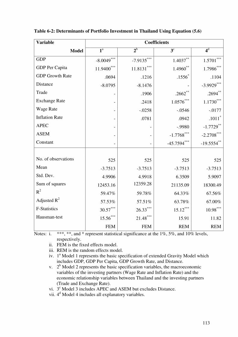
113
Table 6-2: Determinants of Portfolio Investment in Thailand Using Equation (5.6)
Variable Coefficients
Model 1a 2b 3c 4d
GDP -8.0049*** -7.9135*** 1.4037** 1.5701***
GDP Per Capita 11.9400*** 11.8131*** 1.4960** 1.7986***
GDP Growth Rate .0694 .1216 .1556* .1104
Distance -8.0795 -8.1476 - -3.9929***
Trade - .1906 .2662** .2694**
Exchange Rate - .2418 1.0576*** 1.1730***
Wage Rate - -.0258 -.0546 -.0177
Inflation Rate - .0781 .0942 .1011*
APEC - - -.9980 -1.7729**
ASEM - - -1.7768*** -2.2708***
Constant - - -45.7594*** -19.5554**
No. of observations 525 525 525 525
Mean -3.7513 -3.7513 -3.7513 -3.7513
Std. Dev. 4.9906 4.9918 6.3509 5.9097
Sum of squares 12453.16 12359.28 21135.09 18300.49
R2 59.47% 59.78% 64.33% 67.56%
Adjusted R2 57.53% 57.51% 63.78% 67.00%
F-Statistics 30.57*** 26.33*** 15.12*** 10.98***
Hausman-test 15.56*** 21.48*** 15.91 11.82
FEM FEM REM REM
Notes: i. ***, **, and * represent statistical significance at the 1%, 5%, and 10% levels, respectively.
ii. FEM is the fixed effects model. iii. REM is the random effects model.
iv. 1a Model 1 represents the basic specification of extended Gravity Model which includes GDP, GDP Per Capita, GDP Growth Rate, and Distance.
v. 2b Model 2 represents the basic specification variables, the macroeconomic variables of the investing partners (Wage Rate and Inflation Rate) and the economic relationship variables between Thailand and the investing partners (Trade and Exchange Rate).
vi. 3c Model 3 includes APEC and ASEM but excludes Distance. vii. 4d Model 4 includes all explanatory variables.
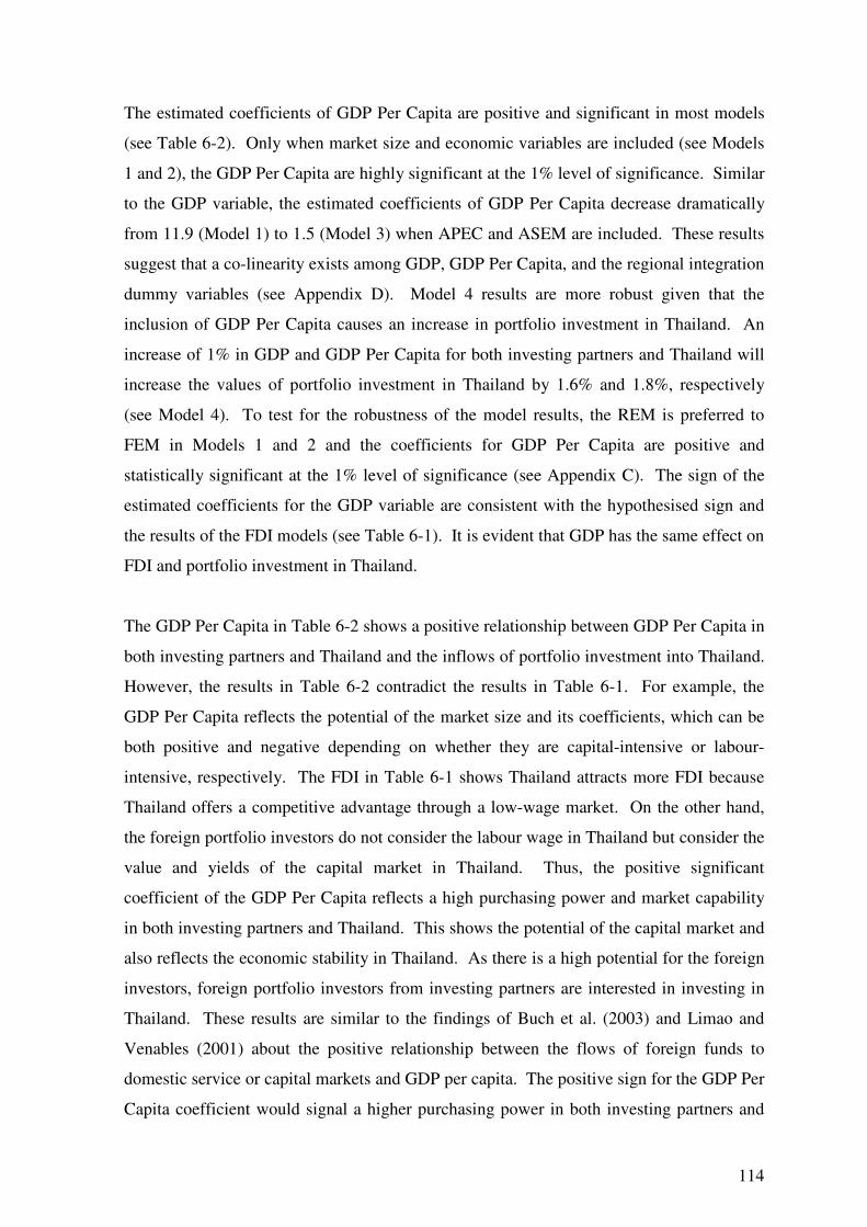
114
The estimated coefficients of GDP Per Capita are positive and significant in most models
(see Table 6-2). Only when market size and economic variables are included (see Models
1 and 2), the GDP Per Capita are highly significant at the 1% level of significance. Similar
to the GDP variable, the estimated coefficients of GDP Per Capita decrease dramatically
from 11.9 (Model 1) to 1.5 (Model 3) when APEC and ASEM are included. These results
suggest that a co-linearity exists among GDP, GDP Per Capita, and the regional integration
dummy variables (see Appendix D). Model 4 results are more robust given that the
inclusion of GDP Per Capita causes an increase in portfolio investment in Thailand. An
increase of 1% in GDP and GDP Per Capita for both investing partners and Thailand will
increase the values of portfolio investment in Thailand by 1.6% and 1.8%, respectively
(see Model 4). To test for the robustness of the model results, the REM is preferred to
FEM in Models 1 and 2 and the coefficients for GDP Per Capita are positive and
statistically significant at the 1% level of significance (see Appendix C). The sign of the
estimated coefficients for the GDP variable are consistent with the hypothesised sign and
the results of the FDI models (see Table 6-1). It is evident that GDP has the same effect on
FDI and portfolio investment in Thailand.
The GDP Per Capita in Table 6-2 shows a positive relationship between GDP Per Capita in
both investing partners and Thailand and the inflows of portfolio investment into Thailand.
However, the results in Table 6-2 contradict the results in Table 6-1. For example, the
GDP Per Capita reflects the potential of the market size and its coefficients, which can be
both positive and negative depending on whether they are capital-intensive or labour-
intensive, respectively. The FDI in Table 6-1 shows Thailand attracts more FDI because
Thailand offers a competitive advantage through a low-wage market. On the other hand,
the foreign portfolio investors do not consider the labour wage in Thailand but consider the
value and yields of the capital market in Thailand. Thus, the positive significant
coefficient of the GDP Per Capita reflects a high purchasing power and market capability
in both investing partners and Thailand. This shows the potential of the capital market and
also reflects the economic stability in Thailand. As there is a high potential for the foreign
investors, foreign portfolio investors from investing partners are interested in investing in
Thailand. These results are similar to the findings of Buch et al. (2003) and Limao and
Venables (2001) about the positive relationship between the flows of foreign funds to
domestic service or capital markets and GDP per capita. The positive sign for the GDP Per
Capita coefficient would signal a higher purchasing power in both investing partners and
115
Thailand. This implies the existence of wealth effects. The rising in purchasing power in
investing partners and Thailand accelerates the expansion of the portfolio investment into
Thailand. Hence, GDP per capita in the investing partners and Thailand has a positive
effect on portfolio investment in Thailand. In comparison, if foreign funds are encouraged
in order to produce overseas exports, the sign of GDP Per Capita coefficient should be
negative due to the relatively low cost of labour in Thailand, which is consistent with the
result in Table 6-1.
GDP Growth Rate is positive in all models and significant at the 10% level of significance
only in Model 3 when Distance is excluded. However, the GDP Growth Rate is not
significantly different from zero in Models 1, 2, and 4. These results imply that GDP
Growth Rates of the investing partners has no influence on portfolio investment in
Thailand (see Model 4). These results are slightly different from the FDI models (see
Table 6-1). This could be due to the indirect effect of the economic environment of the
investing partners, whereas portfolio investment depends only on the strength of Thai
economy and not on external conditions.
The estimated geographical Distance coefficient is negative and statistically significant at
the 1% level of significance in Model 4. Holding other factors constant, an increase in
Distance by 1% would decrease the inflows of portfolio investment in Thailand by 4.0%.
Based on the definition of geographical Distance by Bevan and Estrin (2004), Guerin
(2006), and Portes and Rey (2005), distance may be a proxy for information costs in FDI
and portfolio investment models rather than transport costs in the trade models. Therefore,
information costs of portfolio investment between the investing partners and Thailand are
large and have negative effects on portfolio investment in Thailand. Furthermore, portfolio
investment decreases as the distance from Thailand increases. A significant decrease in
information costs has a positive impact on portfolio investment. On the other hand,
distance has a negative correlation with the flows of portfolio investment. For example,
Singapore and China (including Hong Kong) had the highest percentage of the inflow of
portfolio investment into Thailand during 1980-2004 (see Table 2-5 in Chapter 2). Both
countries are familiar with Thailand’s culture and language although they do not
communicate in the Thai language. This familiarity reduces the information costs between
Singapore, China, and Thailand. The results are consistent with Portes and Rey’s (2005)
116
findings, that foreign investors prefer to invest in markets close to them. This suggests that
the distance is a significant factor in determining portfolio investment in Thailand.
In addition to the information cost, Distance can be a proxy for financial and infrastructure
systems. The negative effects of distance on portfolio investment are also expected to be
due to the differences in the respective countries’ regulations and financial systems and
Thailand’s inferior qualities of infrastructure and communications. The results in Table 6-
2 reveal strong evidence that portfolio investment does not follow the same pattern as FDI.
However, Guerin (2006) suggested that portfolio investment follows the same pattern as
FDI and that the Distance variable in FDI is more significant than in portfolio investment.
Based on the Distance coefficients from Tables 6-1 and 6-2, portfolio investment is more
sensitive to distance than FDI in Thailand.
Trade coefficient is consistent with a priori hypothesised sign but is insignificant in Model
2. The Trade variable is somewhat unstable but it influences the portfolio investment with
the regional integration variables in Models 3 and 4. The Trade coefficients are positive
and significant in Models 3 and 4 at the 5% level of significance. Higher trade volume
brings higher value of portfolio investment from investing partners into Thailand. This
result is similar to the FDI models (see Table 6-1) with a priori hypothesised signs. This
also suggests that portfolio investment flows are to some extent enhanced by trade.
The estimated coefficients of the Exchange Rate variable have a positive effect on
portfolio investment in Thailand, as priori hypothesised, and are statistically significant at
the 1% level of significance in Models 3 and 4. However, the coefficient of Exchange
Rate is statistically insignificant in Model 2. The positive coefficient of the Exchange Rate
indicates that an appreciation of 1% in the exchange rate of the investing partners against
the Thai Baht will increase portfolio investment in Thailand by 1.2% (see Model 4). The
results show that portfolio investment is sensitive to changes in the exchange rate. As the
investing partners’ currencies appreciate, the cost of capital investment in Thailand
becomes cheaper, thus increasing portfolio investment.
The results also show that depreciation of the Thai Baht has a strong positive effect on
portfolio investment. Some investing partners such as Austria, Denmark, France, Italy,
117
Malaysia, Indonesia, Sweden, and South Korea (see Table 2-5, Chapter 2) are not
interested in investing in the Thailand capital market due to the exchange rate instability.
The Thai government initiated liberalisation of financial institutions under WTO
commitments through the Bangkok International Banking Facilities (BIBF) in 1993. The
BIBF enjoys several distinct tax privileges such as a 10% reduction on corporate income
tax (from 30% previously), a 0% rate for specific business tax, interest income withholding
tax, and no duties for investors who invest in Thailand (Siamwalla et al., 1999). In effect,
the BIBF has become a financial intermediary to the manufacturing sector, commerce, and
banking and finance between foreign investors and Thai investors. The volume of net
capital inflows into Thailand surged from approximately US$ 2,400 million (US$ 1,294
million on FDI and US$ 1,100 million on portfolio investment) in 1988 to US$ 21,888
million (US$ 5,142 million on FDI and US$ 21,376 million on portfolio investment) in
1997 (see Chapter 2). In contrast, net inflows plunged to US$ 13,742 million (US$ 6,981
million on FDI and US$ 6,761 million on portfolio investment) in 1998 (see Chapter 2)
after the 1997 Asian Financial Crisis.
The Wage Rate and Inflation Rate of the investing partners are included in Equation (5.6)
to examine the relative impact of macroeconomic factors in investing partners over
Thailand. The Wage Rate estimates for portfolio investment in all models are negative, but
their values are not significantly different from zero. The results in Table 6-2 show that
Wage Rate has no significant impact on portfolio investment in Thailand. This may
suggest that the wage rate of the investing partners did not affect capital outflows to
Thailand during the years 1980-2004.
The Inflation Rate is statistically significant at the 10% level of significance in Model 4, as
priori hypothesised. A high inflation rate in the investing partners indicates the presence
of economic risk in their countries in the long-term (see Chapter 5). A higher inflation rate
may lead to an inducement in outward FDI from investing partners to consider investing in
Thailand. In addition, when foreign investors transfer profits back to their countries they
would benefit if the inflation rate in their countries is high because the currency would
have more value when converted to domestic currencies. In this case, foreign investors’
profits are higher as a result of the appreciated exchange rates. Therefore, the estimated
coefficient of Inflation Rate shows that the inflation rate in investing partners has a
118
significant impact on the determinants of portfolio investment in Thailand during the years
1980-2004 (see Model 4).
Table 6-2 shows that the dummy variables, the membership in APEC and ASEM for
investing partners and Thailand, are both negative and statistically significant. APEC is
negative and significant in Model 4 at the 5% level of significance, but it is insignificant in
Model 3. ASEM is negative and statistically significant at the 1 % level of significance in
Models 3 and 4. When investing partners and Thailand are members of APEC, there is a
less significant impact on portfolio investment than when they are members of ASEM.
APEC and ASEM coefficients were hypothesised as positive (see Chapter 5), but the
results show negative signs. The negative signs for the regional integration dummy
variables are consistent with the results of Biessen (1991), Brenton et al. (1999), and Portes
and Rey (2005). The negative results arise from the fact that investing partners depend on
their own financial resources and their domestic capital markets. In addition, the investing
partners may delay their investment in Thailand until they achieve their objectives such as
tax deduction or tax exemption from the government. Hence, APEC and ASEM members
have undoubtedly affected the investment of the capital markets in Thailand. This
indicates that the co-operation of APEC and ASEM membership as an integrated scheme
determines the portfolio investment in Thailand. This is consistent with the results of
Cuevas et al. (2005), that the negative significant regional integration variables means an
investing country would delay investment until the host country provides exceptional
investment incentives. The result may reflect that foreign investors may change their
investment plan while making their investment decisions. That is, depending on the
investment environment, foreign investors may decide to invest in the manufacturing
sectors instead of capital investment. Investors in general preferred to invest in countries
who are members of APEC and ASEM. This may be because APEC and ASEM believe
that direct investment can increase countries’ welfare and sustain economic growth to the
host countries through the increase of job opportunities, skill improvement, technology
transfer, and poverty reduction.
The regional integration variables are negatively significant in the portfolio investment
model (see Table 6-2), but positive in the FDI model (see Table 6-1). The significant
119
negative signs of APEC and ASEM variables in Table 6-2 indicate negative impacts on the
flows of portfolio investment into Thailand. Foreign investors may shift their funds to
direct investment such as the manufacturing sector because they can gain benefits from the
APEC and ASEM agreements (see Table 6-1). APEC and ASEM members focus more
efficiently on reducing production and transaction costs, improving trade information and
business policies in order to increase trade and to provide cheaper goods and services with
more employment opportunities. The APEC and ASEM achievement stem from the
expanded economies and facilitates economic growth among members (Chadee and
Schlichting, 1997).
The overall results in Table 6-2 show that GDP, GDP Per Capita, Distance, Trade,
Exchange Rate, APEC, and ASEM variables are important factors affecting the size of
portfolio investment in Thailand (see Model 4). The significant positive estimate of GDP
is a basic specification of the economic determinant in the portfolio investment model.
The coefficients of GDP Growth Rate and Wage Rate are not significantly different from
zero in all models and do not have significant impacts on the amount of portfolio
investment. However, the negative significant coefficient of Distance indicates that
portfolio investment is determined by the gravity factor.
The Wage Rate variable is not significantly different from zero in all models. The GDP
Growth Rate is significant only in Model 3 at the 10% level of significance. The Inflation
Rate is significant only in Model 4 at the 10% level of significance. The estimated
coefficients of these three variables are small. This shows that the economic status of
investing partners does not appear to influence portfolio investment, and suggests that
portfolio investment into Thailand is mainly driven by the internal economic status. For
example, there is a wealth effect due to the devaluation of the Thai Baht driving up the
inflows of portfolio investment into Thailand. Moreover, from the empirical results in
Table 6-2, it is evident that portfolio investment in Thailand does not follow the FDI
pattern.
6.3 The Effects of the 1997 Asian Financial Crisis on FDI and Portfolio Investment in Thailand
Before 1997, the strong economic growth and attractive stock returns in Thailand attracted
foreign investors to relocate their funds to the financial and capital markets in Thailand.
120
Thailand was one of the countries in Asia which benefited from strong economic growth as
the results of globalisation, international financial linkages, and expansion of production
bases overseas from investing countries. For example, the aggregate volume of net capital
inflows into Thailand surged from US$ 6.4 billion in 1990 to US$ 26.4 billion in 1997.
However, these net inflows fell to US$ 13.6 billion in 1998 after Thailand was badly
affected by the Asian Financial Crisis in mid 1997.
The financial sector was already weak before the floating of the Thai Baht on 2 July, 1997,
and 58 finance companies were suspended in the second half of 1997 (Sussangkarn, 1999).
The Asian Financial Crisis almost crippled Thailand economy. The exchange rate
depreciated from 25 Baht per US Dollar in December, 1996 to 52 Baht per US Dollar in
December, 1997. In addition, the gross domestic investment (GDI) decreased dramatically
from US$ 76.2 billion, to US$ 50.7 billion and US$ 22.9 billion in 1996, 1997 and 1998,
respectively (see Table 2-1). However, the current account balance turned into a
substantial surplus in 1998 after decades of negative. The depreciation of the Baht has
caused the export of manufactured products to increase dramatically while the level of
import capital goods and materials dropped. This led to the current account surplus.
Consequently, the 1997 Asian Financial Crisis might cause substantial changes in the FDI
and portfolio investment in Thailand.
In the second half of 1997, financial chaos erupted in the Thai economy. Large amounts of
short-term foreign debt was repaid which affected Thailand. However, FDI and portfolio
inflows remained positive; inflows in 1997 and 1998 to Thailand were similar to those of
1996. In 1998, however, they fell by 31.6% (see Table 2-1); inflows became low or
negative because of the political instability and economic adjustment problems. To test
for the effects of the 1997 Asian Financial Crisis, this study includes dummy variables to
represent the years of Asian Financial Crisis. Following Perron (1989) and Zhou and
Lall’s (2005) studies, we extended estimating Equations (5.5) and (5.6) by including Dt
equal to one for 1997 and 1998, the years when the Asian Financial Crisis was at its peak
(1997 and 1998). Equation (5.10) captures the structural break for FDI models in
Thailand. Finally, the break for portfolio flows in Thailand can be captured by Equation
(5.11).
121
6.3.1 Structural Break in FDI Models in Thailand
Model 1 in Table 3 shows the estimated coefficients of the extended Gravity Models which
consist of the size of the market (GDP, GDP Per Capita, and GDP Growth Rate), the
geographical Distance and the Asian Financial Crisis dummy variables (1997 and 1998).
Model 2 expands the regression shown in Model 1 with additional economic environment
variables such as Trade, Exchange Rate, Wage Rate, and Inflation Rate. It examines the
effects of investing partners’ economies on the inflows of FDI into Thailand. The APEC
and ASEM variables are included in Models 3 and 4 to determine whether externalities
generated by the regional integrations provide an additional impetus to the inflows of FDI
into Thailand. However, Model 3 differs from Model 4 by excluding the Distance variable
to examine the gravity specification in the determinants of FDI into Thailand. Hence,
Model 4 shows the empirical results for all explanatory variables including the Asian
Financial Crisis dummy variables.
In general, the coefficients for all the variables (except the Asian Financial Crisis dummy
variables) are consistent with the results in Table 6-1 (see Table 6-3). When the Asian
Financial Crisis dummy variables are added the results of the F-statistics and Breusch and
Pagan tests fail to accept the null hypotheses of common intercept. The Hausman test is
used to test whether the FEM or REM is preferred. The results of the Hausman test fail to
accept the null hypothesis. Therefore, all models that accept the FEM are significant at the
1% level of significance. The results show the FEMs are preferred to the random effects
models (REM) as suggested by the Hausman tests. However, Model 2 could not be tested
using the Hausman tests because the data could not invert the Variance-Covariance matrix
for the Hausman test. This is because the variances are not constant and the covariances
are not equal to zero under the assumptions of the random effects structure (Wooldridge,
2002). There might be concerns about multicollinearity between the Asian Financial Crisis
dummy variables. The correlation between the two Asian Financial Crisis dummy
variables is not disturbingly high (see Appendix D). The fact that the Asian Financial
Crisis dummy variables are jointly significant suggests that each of the variables detected
the existence of financial crisis asymmetries across countries. Therefore, these regressions
have to accept the fixed effects models which contain higher R2 values than the OLS
regressions and show statistically significant group (country) effects. The explanatory
powers of all four models (R2) are very high, between 70%-72%, especially in Models 3
and 4 which contain 72%.

122
Table 6-3: Determinants of FDI in Thailand Using Equation (5.10)
Variable Coefficients
Model 1a 2 b 3 c 4 d
GDP 4.4548*** 4.5761*** 4.0982*** 4.0982***
GDP Per Capita -3.6163*** -3.6130*** -3.1036** -3.1036**
GDP Growth Rate .0263 .0702** .0822** .0822**
Distance .3582 .1503 - -.0391
Trade - .0985** .1139** .1139**
Exchange Rate - -.4043* -.5223** -.5223**
Wage Rate - .1102** .1194** .1194**
Inflation Rate - .0765*** .0860*** .0860***
APEC - - -.3924 -.3924
ASEM - - .6265** .6265**
Dummy 1997 .1019 .0620 -.1792 -.1792
Dummy 1998 .8090** .8556** .6706 .6706
Constant - - -
-
No. of observations 525 525 525 525
Mean 2.0851 2.0851 2.0851 2.0851
Std. Dev. 1.7950 1.7578 1.7429 1.7446
Sum of squares 1604.58 1526.41 1497.49 1497.49
R2 69.55% 71.04% 71.58% 71.58%
Adjusted R2 67.96% 69.28% 69.80% 69.74%
F-Statistics 43.75*** 40.38*** 40.06*** 38.73***
Hausman-test 29.43*** -e 35.63*** 40.31***
FEM FEM FEM FEM
Notes: i. ***, **, and * represent statistical significance at the 1%, 5% and 10% levels, respectively.
ii. FEM is the fixed effects model. iii. 1a Model 1 represents the basic specification of extended Gravity Model which
includes GDP, GDP Per Capita, GDP Growth Rate, and Distance. iv. 2b Model 2 represents the basic specification variables, the macroeconomic
variables of the investing partners (Wage Rate and Inflation Rate) and the economic relationship variables between Thailand and investing partners (Trade and Exchange Rate).
v. 3c Model 3 includes APEC and ASEM but excludes Distance. vi. 4d Model 4 includes all explanatory variables.
vii. e Model 2 shows the regression which could not invert the Variance-Covariance matrix for the Hausman test.
123
All variables in Table 6-3 have the hypothesised signs except Exchange Rate (Models 2, 3,
and 4), Distance (Model 1), and APEC (Models 3 and 4). However, Distance and APEC
coefficients are not significantly different from zero at the 10% level of significance. The
coefficients of GDP, GDP Per Capita, GDP Growth Rate, Trade, Wage Rate, Inflation
Rate, and ASEM have the hypothesised signs and are statistically significant. Exchange
Rate contradicts prior hypothesised sign but is statistically significant at the 10% level of
significance in Model 2 and at the 5% level of significance in Models 3 and 4. There are
three reasons for this contradictive hypothesised signs (see Section 6.1): (1) investors take
advantage of importing components, parts, and raw material from overseas; (2) most FDIs
go to non-industry sectors; and (3) increase the confidence of the Thai economic status in
the lone term. Therefore, the results for Exchange Rate show an opposite of the prior
hypothesised sign.
The Asian Financial Crisis dummy variables are statistically insignificant in Models 3 and
4. Thus, the dummy variables of Asian Financial Crisis do not have a significant effect on
FDI inflows into Thailand. This suggests that the inflows of FDI into Thailand were not
affected by the 1997 Asian Financial Crisis and the economic depression during 1997-
1998. Table 2-2 (Chapter 2) shows evidence that FDI inflows into Thailand grew steadily
in 1997-1998 after the Baht was floated (US$ 3.9 billion in 1996, US$ 5.1 billion in 1997,
and US$ 6.9 billion in 1998). This could have been attributed to a large number of
ongoing projects approved by BOI, which are long-term commitments. The inflows of
FDI into Thailand were stable during the 1997 Asian Financial Crisis. In order for the FDI
to exit Thailand, the MNCs must either be sold or shut down, which would likely occur in
time of severe recession and if foreign investors intend to leave Thailand permanently. To
check the robustness of the effects of the Asian Financial Crisis, the 1999 dummy variable
was included into the FDI models. The result shows that the 1999 dummy variable has no
impact on FDI. However, if the Asian Financial Crisis has an effect on the FDI inflows
then the FDI was withdrawn or deposited by foreign investors in Thailand in 1997 and
1998 but these funds have been restored by 1999.
The Asian Financial Crisis dummy variables are included in the models (see Table 6-3)
and the results are similar to the results in Table 6-1 without significant changes of the
coefficients’ magnitudes in all variables (except the 1997 and 1998 dummy variables
which are presented in Table 6-3 only). This may be because the Asian Financial Crisis
124
dummy variables have no significant effect on the FDI models. The GDP and GDP Per
Capita variables are highly significant to the inflows of FDI into Thailand in both a
positive and negative direction, respectively, in all models (see Table 6-3). Trade and
Wage Rate are positive and significant at the 5% level of significance in all models.
Inflation Rate has a positive effect on the flows of FDI into Thailand at the 1% level of
significance in all models. The estimated coefficients of Exchange Rate are negative and
significant at the 10%, 5%, and 5% level of significance in Models 2, 3, and 4,
respectively. The findings show that the ASEM agreement positively affects the
determinants of FDI in Thailand at the 5% level of significance in Models 3 and 4. The
Asian Financial Crisis dummy variables are not significantly different from zero in Models
3 and 4. The results in Table 6-3 are consistent with those in Table 6-1. This suggests that
the Asian Financial Crisis dummy variables do not significantly affect the inflows of FDI
into Thailand (see Models 3 and 4). However, the significant Exchange Rate variable
shows that the determinants of FDI in Thailand are sensitive to changes in the economic
depression and the depreciation of Thai Baht during the 1997 Asian Financial Crisis.
The estimated coefficients of GDP are positive and statistically significant at the 1% level
of significance in all models. This highlights the importance of investing partners’ and
Thailand’s production capacities in encouraging the inflows of FDI into Thailand. In
addition, the positive sign on the GDP Growth Rate variable in Models 2, 3 and 4 shows
the strength of investing partners’ economies positively affecting the inflows of FDI into
Thailand. As expected, the inflows of FDI into Thailand increase with GDP and GDP
Growth Rate. However, the negative coefficient on GDP Per Capita is consistent with the
result in Table 6-1 and the hypothesis that Thailand is a labour-intensive country rather
than a capital-intensive country. This implies that when FDI invest in Thailand, they
prefer a reduction in production costs through labour costs. This implies that Thailand had
shifted resources from traditional agriculture to labour-intensive manufacturing in the
1990s (see Table 2-3).
As more economic environment variables such as Trade, Exchange Rate, Wage Rate, and
Inflation Rate are included in Model 2, the estimated results show all variables are
statistically significant. Thus, holding other variables constant, the inflows of FDI into
Thailand are very responsive to the economic environment with respect to investing
partners’ economies. The results indicate that the financial crisis that burst in mid-1997 in
125
Thailand had ended by 1999. The positive coefficient sign of 1998 dummy variable
suggests that the crisis had encouraged the inflows of FDI into Thailand and perhaps had
contributed to Thailand’s rapid recovery from economic depression. The estimated signs
for Distance contradict the hypothesised sign, but the coefficient is not significantly
different from zero. The results from Model 1 show that GDP Growth Rate and Distance
have no significant impact on the inflows of FDI into Thailand and the years 1997 dummy
variable yields an insignificant relationship to the inflows of FDI into Thailand.
The Distance variable, which is a part of the extended Gravity Model, is included in Model
4 to test the effect of information or transaction costs on the inflows of FDI into Thailand.
The results of Model 3 (without Distance variable) and Model 4 (with Distance variable)
show similar results. This indicates that the Distance in Table 6-3 has no impact on the
inflows of FDI into Thailand. It is evident that distance does not play an important role in
FDI decisions by foreign investors even when the Asian Financial Crisis dummy variables
are included in the model. The investing partners and Thailand have different legal
systems, culture, and infrastructure which do not significantly determine the inflows of
FDI into Thailand. As discussed earlier, distance is a proxy for information or transaction
costs, therefore, either the information or transaction costs do not significantly affect to the
FDI or FDI is not sensitive to the distance.
The coefficients of the Trade variable are positive and statistically significant at the 5%
level of significance in Models 2, 3, and 4. This shows that trade between investing
partners and Thailand has a positive effect on the inflows of FDI into Thailand. The
results are consistent with the results in Table 6-1 and confirm that FDI and Trade between
the investing partners and Thailand are complementary even when the Asian Financial
Crisis dummy variables are included in the models.
The estimated coefficients of Exchange Rate are negative and statistically significant at the
10%, 5%, and 5% level of significance in Models 2, 3, and 4, respectively. Compared to
the Exchange Rate estimates in Model 2 in Table 6-1, the estimated coefficient of
Exchange Rate is significant in Table 6-3 only when the Asian Financial Crisis dummy
variables are included. The negative sign of Exchange Rate is discussed in Section 6.1 and
it shows that a depreciation of investing partners’ currencies against the Thai Baht,
encourages the inflow of FDI into Thailand. In Model 1 (see Table 6-3), the 1998 dummy
126
variable has a positive effect on the inflows of FDI into Thailand. This coincides with the
Asian Financial Crisis in mid-1997. In addition, both Exchange Rate and 1998 dummy
variables are statistically significant, hence, suggesting a strong correlation between the
exchange rate and the Asian Financial Crisis in Thailand. Thailand floated the Baht in July
1997; the surplus in the balance of current account generated an additional net foreign
exchange inflow into Thailand of about US$ 2 billion per month (Sussangkarn, 1999). The
current account continued to be in surplus throughout 1998, with the accumulated surplus
totalling about US$ 14.3 billion (see Table 2-1). As the current account surplus
accumulated, Thailand began to strengthen its exports and received US$ 7 billion of FDI in
1998 (see Table 2-1). Furthermore, the depreciation of the Thai Baht and the current
account surplus regained market share for Thai products in the global market and reassured
foreign investors of Thailand’s position to meet its world competitiveness. Consequently,
the massive amounts of FDI especially in 1998 helped the country to recover from the
1997 Asian Financial Crisis.
The coefficients of Wage Rate are positive and statistically significant at the 5% level of
significance in Models 2, 3, and 4. The coefficients of Inflation Rate are positive and
statistically significant at the 1% level of significance in Models 2, 3, and 4. This is
consistent with the results in Table 6-1, suggesting the 1997 Asian Financial Crisis in
Thailand had no significant effect on the investing partners’ decisions to invest in
Thailand. Wage Rate and Inflation Rate in Table 6-3 indicate the macroeconomic climate
of the investing partners. Therefore, the results show that high labour wage and high
inflation rate in investing partners can encourage outward FDI and increase FDI into
Thailand. In 1996-8, the minimum wage rate in Thailand was 157 Baht per day (TDRI,
2003), which became cheaper after the depreciation of the Thai Baht in mid 1997. This
caused the wage rate in investing partners to become more expensive compared to
Thailand’s minimum wage rate. Therefore, the investing partners take advantage of this by
increasing the outward FDI to other countries, such as Thailand and Indonesia, which were
hit by the Asian Financial Crisis. The findings support the hypothesis that wage rate has
positive effects on FDI into Thailand. This is consistent with Yilmaz’s (2001) findings and
the results in Model 2 (see Table 6-1) that the determinants of FDI into Thailand are
mainly driven by the economic status in the investing partners.
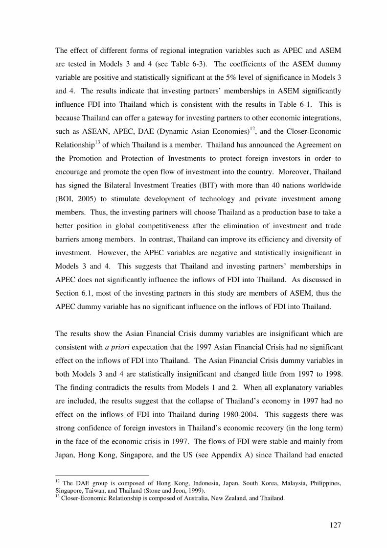
127
The effect of different forms of regional integration variables such as APEC and ASEM
are tested in Models 3 and 4 (see Table 6-3). The coefficients of the ASEM dummy
variable are positive and statistically significant at the 5% level of significance in Models 3
and 4. The results indicate that investing partners’ memberships in ASEM significantly
influence FDI into Thailand which is consistent with the results in Table 6-1. This is
because Thailand can offer a gateway for investing partners to other economic integrations,
such as ASEAN, APEC, DAE (Dynamic Asian Economies)12, and the Closer-Economic
Relationship13 of which Thailand is a member. Thailand has announced the Agreement on
the Promotion and Protection of Investments to protect foreign investors in order to
encourage and promote the open flow of investment into the country. Moreover, Thailand
has signed the Bilateral Investment Treaties (BIT) with more than 40 nations worldwide
(BOI, 2005) to stimulate development of technology and private investment among
members. Thus, the investing partners will choose Thailand as a production base to take a
better position in global competitiveness after the elimination of investment and trade
barriers among members. In contrast, Thailand can improve its efficiency and diversity of
investment. However, the APEC variables are negative and statistically insignificant in
Models 3 and 4. This suggests that Thailand and investing partners’ memberships in
APEC does not significantly influence the inflows of FDI into Thailand. As discussed in
Section 6.1, most of the investing partners in this study are members of ASEM, thus the
APEC dummy variable has no significant influence on the inflows of FDI into Thailand.
The results show the Asian Financial Crisis dummy variables are insignificant which are
consistent with a priori expectation that the 1997 Asian Financial Crisis had no significant
effect on the inflows of FDI into Thailand. The Asian Financial Crisis dummy variables in
both Models 3 and 4 are statistically insignificant and changed little from 1997 to 1998.
The finding contradicts the results from Models 1 and 2. When all explanatory variables
are included, the results suggest that the collapse of Thailand’s economy in 1997 had no
effect on the inflows of FDI into Thailand during 1980-2004. This suggests there was
strong confidence of foreign investors in Thailand’s economic recovery (in the long term)
in the face of the economic crisis in 1997. The flows of FDI were stable and mainly from
Japan, Hong Kong, Singapore, and the US (see Appendix A) since Thailand had enacted
12 The DAE group is composed of Hong Kong, Indonesia, Japan, South Korea, Malaysia, Philippines, Singapore, Taiwan, and Thailand (Stone and Jeon, 1999). 13 Closer-Economic Relationship is composed of Australia, New Zealand, and Thailand.
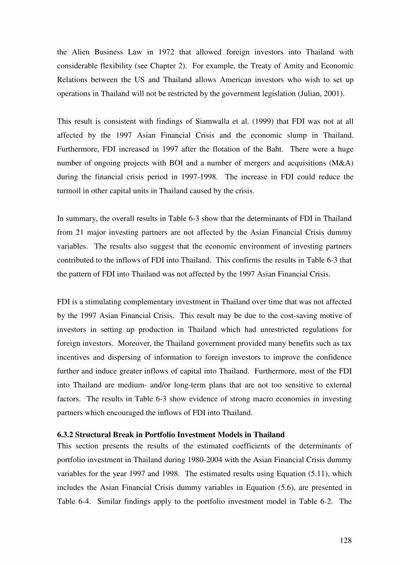
128
the Alien Business Law in 1972 that allowed foreign investors into Thailand with
considerable flexibility (see Chapter 2). For example, the Treaty of Amity and Economic
Relations between the US and Thailand allows American investors who wish to set up
operations in Thailand will not be restricted by the government legislation (Julian, 2001).
This result is consistent with findings of Siamwalla et al. (1999) that FDI was not at all
affected by the 1997 Asian Financial Crisis and the economic slump in Thailand.
Furthermore, FDI increased in 1997 after the flotation of the Baht. There were a huge
number of ongoing projects with BOI and a number of mergers and acquisitions (M&A)
during the financial crisis period in 1997-1998. The increase in FDI could reduce the
turmoil in other capital units in Thailand caused by the crisis.
In summary, the overall results in Table 6-3 show that the determinants of FDI in Thailand
from 21 major investing partners are not affected by the Asian Financial Crisis dummy
variables. The results also suggest that the economic environment of investing partners
contributed to the inflows of FDI into Thailand. This confirms the results in Table 6-3 that
the pattern of FDI into Thailand was not affected by the 1997 Asian Financial Crisis.
FDI is a stimulating complementary investment in Thailand over time that was not affected
by the 1997 Asian Financial Crisis. This result may be due to the cost-saving motive of
investors in setting up production in Thailand which had unrestricted regulations for
foreign investors. Moreover, the Thailand government provided many benefits such as tax
incentives and dispersing of information to foreign investors to improve the confidence
further and induce greater inflows of capital into Thailand. Furthermore, most of the FDI
into Thailand are medium- and/or long-term plans that are not too sensitive to external
factors. The results in Table 6-3 show evidence of strong macro economies in investing
partners which encouraged the inflows of FDI into Thailand.
6.3.2 Structural Break in Portfolio Investment Models in Thailand
This section presents the results of the estimated coefficients of the determinants of
portfolio investment in Thailand during 1980-2004 with the Asian Financial Crisis dummy
variables for the year 1997 and 1998. The estimated results using Equation (5.11), which
includes the Asian Financial Crisis dummy variables in Equation (5.6), are presented in
Table 6-4. Similar findings apply to the portfolio investment model in Table 6-2. The
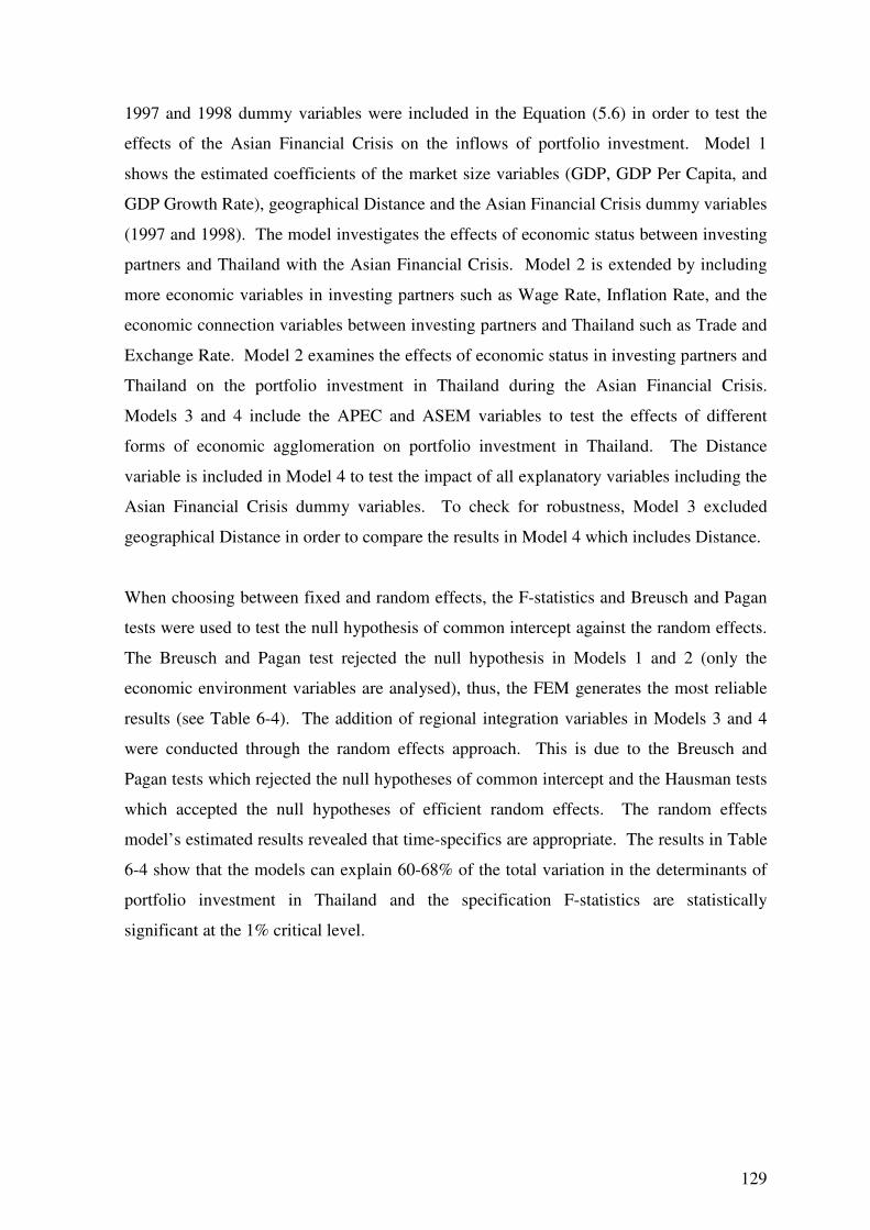
129
1997 and 1998 dummy variables were included in the Equation (5.6) in order to test the
effects of the Asian Financial Crisis on the inflows of portfolio investment. Model 1
shows the estimated coefficients of the market size variables (GDP, GDP Per Capita, and
GDP Growth Rate), geographical Distance and the Asian Financial Crisis dummy variables
(1997 and 1998). The model investigates the effects of economic status between investing
partners and Thailand with the Asian Financial Crisis. Model 2 is extended by including
more economic variables in investing partners such as Wage Rate, Inflation Rate, and the
economic connection variables between investing partners and Thailand such as Trade and
Exchange Rate. Model 2 examines the effects of economic status in investing partners and
Thailand on the portfolio investment in Thailand during the Asian Financial Crisis.
Models 3 and 4 include the APEC and ASEM variables to test the effects of different
forms of economic agglomeration on portfolio investment in Thailand. The Distance
variable is included in Model 4 to test the impact of all explanatory variables including the
Asian Financial Crisis dummy variables. To check for robustness, Model 3 excluded
geographical Distance in order to compare the results in Model 4 which includes Distance.
When choosing between fixed and random effects, the F-statistics and Breusch and Pagan
tests were used to test the null hypothesis of common intercept against the random effects.
The Breusch and Pagan test rejected the null hypothesis in Models 1 and 2 (only the
economic environment variables are analysed), thus, the FEM generates the most reliable
results (see Table 6-4). The addition of regional integration variables in Models 3 and 4
were conducted through the random effects approach. This is due to the Breusch and
Pagan tests which rejected the null hypotheses of common intercept and the Hausman tests
which accepted the null hypotheses of efficient random effects. The random effects
model’s estimated results revealed that time-specifics are appropriate. The results in Table
6-4 show that the models can explain 60-68% of the total variation in the determinants of
portfolio investment in Thailand and the specification F-statistics are statistically
significant at the 1% critical level.
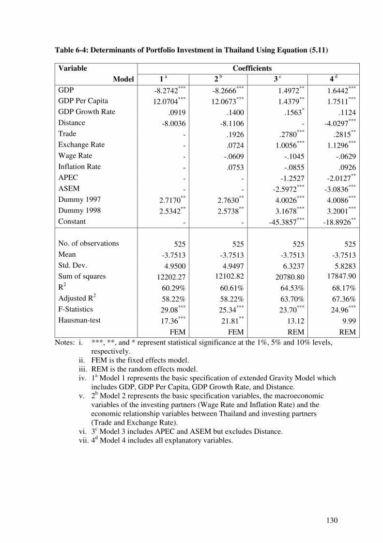
130
Table 6-4: Determinants of Portfolio Investment in Thailand Using Equation (5.11)
Variable Coefficients
Model 1 a 2 b 3 c 4 d
GDP -8.2742*** -8.2666*** 1.4972** 1.6442***
GDP Per Capita 12.0704*** 12.0673*** 1.4379** 1.7511***
GDP Growth Rate .0919 .1400 .1563* .1124
Distance -8.0036 -8.1106 - -4.0297***
Trade - .1926 .2780*** .2815**
Exchange Rate - .0724 1.0056*** 1.1296***
Wage Rate - -.0609 -.1045 -.0629
Inflation Rate - .0753 -.0855 .0926
APEC - - -1.2527 -2.0127**
ASEM - - -2.5972*** -3.0836***
Dummy 1997 2.7170** 2.7630** 4.0026*** 4.0086***
Dummy 1998 2.5342** 2.5738** 3.1678*** 3.2001***
Constant - - -45.3857*** -18.8926**
No. of observations 525 525 525 525
Mean -3.7513 -3.7513 -3.7513 -3.7513
Std. Dev. 4.9500 4.9497 6.3237 5.8283
Sum of squares 12202.27 12102.82 20780.80 17847.90 . R2
60.29% 60.61% 64.53% 68.17%
Adjusted R2 58.22% 58.22% 63.70% 67.36%
F-Statistics 29.08*** 25.34*** 23.70*** 24.96***
Hausman-test 17.36*** 21.81** 13.12 9.99
FEM FEM REM REM
Notes: i. ***, **, and * represent statistical significance at the 1%, 5% and 10% levels, respectively.
ii. FEM is the fixed effects model. iii. REM is the random effects model. iv. 1a Model 1 represents the basic specification of extended Gravity Model which
includes GDP, GDP Per Capita, GDP Growth Rate, and Distance. v. 2b Model 2 represents the basic specification variables, the macroeconomic
variables of the investing partners (Wage Rate and Inflation Rate) and the economic relationship variables between Thailand and investing partners (Trade and Exchange Rate).
vi. 3c Model 3 includes APEC and ASEM but excludes Distance. vii. 4d Model 4 includes all explanatory variables.
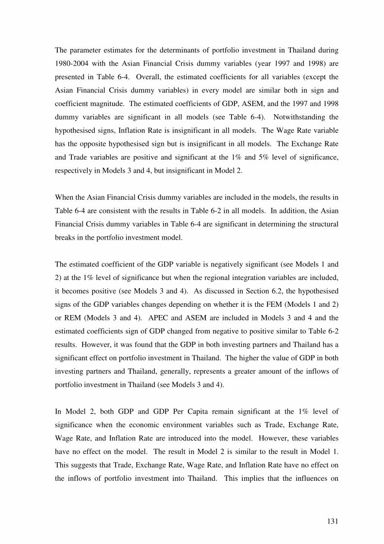
131
The parameter estimates for the determinants of portfolio investment in Thailand during
1980-2004 with the Asian Financial Crisis dummy variables (year 1997 and 1998) are
presented in Table 6-4. Overall, the estimated coefficients for all variables (except the
Asian Financial Crisis dummy variables) in every model are similar both in sign and
coefficient magnitude. The estimated coefficients of GDP, ASEM, and the 1997 and 1998
dummy variables are significant in all models (see Table 6-4). Notwithstanding the
hypothesised signs, Inflation Rate is insignificant in all models. The Wage Rate variable
has the opposite hypothesised sign but is insignificant in all models. The Exchange Rate
and Trade variables are positive and significant at the 1% and 5% level of significance,
respectively in Models 3 and 4, but insignificant in Model 2.
When the Asian Financial Crisis dummy variables are included in the models, the results in
Table 6-4 are consistent with the results in Table 6-2 in all models. In addition, the Asian
Financial Crisis dummy variables in Table 6-4 are significant in determining the structural
breaks in the portfolio investment model.
The estimated coefficient of the GDP variable is negatively significant (see Models 1 and
2) at the 1% level of significance but when the regional integration variables are included,
it becomes positive (see Models 3 and 4). As discussed in Section 6.2, the hypothesised
signs of the GDP variables changes depending on whether it is the FEM (Models 1 and 2)
or REM (Models 3 and 4). APEC and ASEM are included in Models 3 and 4 and the
estimated coefficients sign of GDP changed from negative to positive similar to Table 6-2
results. However, it was found that the GDP in both investing partners and Thailand has a
significant effect on portfolio investment in Thailand. The higher the value of GDP in both
investing partners and Thailand, generally, represents a greater amount of the inflows of
portfolio investment in Thailand (see Models 3 and 4).
In Model 2, both GDP and GDP Per Capita remain significant at the 1% level of
significance when the economic environment variables such as Trade, Exchange Rate,
Wage Rate, and Inflation Rate are introduced into the model. However, these variables
have no effect on the model. The result in Model 2 is similar to the result in Model 1.
This suggests that Trade, Exchange Rate, Wage Rate, and Inflation Rate have no effect on
the inflows of portfolio investment into Thailand. This implies that the influences on
132
portfolio investment in Thailand could not be determined by the economic environment in
investing partners.
The inflows of portfolio investment into Thailand displayed a positive relationship
between GDP, GDP Per Capita, Trade, and Exchange Rate (see Model 4). These results
are consistent with the results in Model 4 in Table 6-2. For example, an increase in
Exchange Rate by 1% will increase the portfolio investment in Thailand by 1.1%,
assuming other factors are held constant. The positive estimated coefficient sign on
Exchange Rate is consistent with Model 4 in Table 6-2. This suggests that the exchange
rate has a positive effect on portfolio investment in Thailand, whereby the appreciation of
investing partner’s currencies against Thai Baht will increase inflow of portfolio
investment into Thailand.
Distance has negative signs in all models but is significant only in Model 4. As shown in
Model 4, the distance between investing partners and Thailand seems to have a negative
significance in foreign portfolio investors’ decision-making about Thailand. Moreover,
Distance also significantly affects the GDP Growth Rate and APEC (see Model 4). It is
evident that geographical distance between investing partners and Thailand is a significant
resistance factor for portfolio investment into Thailand. The inclusion of Distance in
Model 4 increases the magnitude of most coefficients compared to the results in Model 3.
The results confirm that APEC and ASEM are negative and statistically significant at the
5% and 1% level of significance, respectively (see Model 4) which is a similar to Model 4
results (see Table 6-2). The negative sign on APEC and ASEM may be due to the main
objectives of these regional integrations, which are focused on direct investment, but the
results show that regional integrations significantly affect portfolio inflow patterns into
Thailand. Hence, APEC and ASEM will reconsider its members’ interests such as
exchanging views on the global economic outlook and improving the principles and
regulations in the financial sector to enhance investment opportunities amongst members.
The 1997 and 1998 dummy variables are positive and statistically significant at the 5%
level of significance in Models 1 and 2 and the 1% level of significance in Models 3 and 4.
The result supports the hypothesis that the Asian Financial Crisis affected the inflows of
portfolio investment into Thailand. The Asian Financial Crisis dummy variables (1997
133
and 1998 dummy variables) displayed positive impacts on the inflows of portfolio
investment into Thailand. The 1997 and 1998 dummy variables are positive and
significant in all regressions that coincide with the Asian Financial Crisis. This shows the
break in the portfolio investment models which coincides with the Asian Financial Crisis
on the 2nd of July, 1997. The results indicate the positive effect of the Asian Financial
Crisis on portfolio investment in 1997 that was sustained in 1998. The 1997 dummy
variable shows a positive impact of the Asian Financial Crisis on the portfolio investment
in Thailand which means the inflows of portfolio investment into Thailand increased in
1997. Table 2-2 (Chapter 2) shows the dramatic increase in the inflows of portfolio
investment into Thailand from US$ 7,261 million in 1996 to US$ 21,376 million in 1997.
Furthermore, the 1998 dummy variable is positive and significant in the portfolio
investment model (see Model 4). This positive impact is also extended into 1998, by
which time the crisis is highly correlated with the depreciation of Thai Baht. The inflows
of portfolio investment into Thailand in 1998 dropped from 150% from 1997 but the
average inflows of portfolio investment in pre- and post-crisis (1980-1996 and 1999-2004,
respectively) are less than the amount of inflow in 1998, which is US$ 6,761 million. For
example, Table 2-2 (see Chapter 2) shows the average inflows of portfolio investment into
Thailand per year from 1980-1996 (pre-crisis) was US$ 2,418.53 million compared to US$
4,027 million in the post-crisis period (1999-2004). The results in all models (see Table 6-
4) demonstrate that the effect of the Asian Financial Crisis had significant impact on the
inflows of foreign portfolio investment in Thailand in 1997 and 1998. The results indicate
that the occurrence of the financial crisis that burst in mid 1997 in Thailand had significant
impacts on the portfolio investment into Thailand.
The coefficients of Wage Rate and Inflation Rate are not significant in any model (see
Table 6-4). However, the coefficients of the GDP, GDP Per Capita, Distance, Trade,
Exchange Rate, APEC, and ASEM variables are statistically significant but vary in sign
and magnitude in most models. This implies that the inflows of portfolio investment into
Thailand are not driven by the market size and income in the investing partners any more
than by those in Thailand. It suggests that the portfolio investment activity is different
from FDI activity in Thailand. The 1997 and 1998 Asian Financial Crisis dummy
variables are positively significant in the portfolio investment model. Between 1996 and
1997 (pre and post the 1997 Asian Financial Crisis), the flows of portfolio investment into
Thailand increased from US$ 7.3 billion to US$ 21.4 billion in 1997, an increase of more
134
than US$ 14 billion. Conversely, FDI inflows to Thailand increased only US$ 1.2 billion
from 1996 to 1997 (see Table 2-2). Portfolio investment into Thailand responds
significantly to distance and was affected by the Asian Financial Crisis in 1997. The
speculative assault on the Thai currency in July 1997 had a deteriorating impact on the
economy and currency.
6.4 Relationship between FDI and Industrial Categories across Thailand during 1980-2004
This section discusses the industry-level and inward FDI from the 21 Thailand investing
partners between 1980 and 2004. Table 6-5 shows the results of FDI by industrial category
for Thailand using Equation (5.16). The coefficients of the GDP, Capital Stock, Inflation
Rate, Exchange Rate, International Reserves, Wage Rate, Unemployment Rate, Current
Account Balance, National Saving, ASEM and APEC variables for the nine industrial
categories (industry, financial institutions, trade, mining and quarrying, agricultural
products, services, investment, real estate, and others) are estimated using panel data for
Thailand.
The Durbin-Watson tests show no presence of autocorrelation (Greene, 2003). All the
industrial categories have relatively high explanatory power (R2). The F-test failed to
accept the null hypothesis that the estimated parameters for all categories are equal to zero
(see Table 6-5).
The estimated results of the inflows of FDI into Thailand in the industry category perform
satisfactorily; there was a high R2 (95.21%) for all estimates (see Table 6-5). GDP and
Capital Stock are positive and significant at the 1% level of significance. This shows that
the inflows of FDI into the industry category are significant and positively affected by
GDP and Capital Stock. In addition, the Unemployment Rate is positive and statistically
significant at the 5% level of significance. That means a high unemployment rate in
Thailand exerts a positive influence on the inflows of FDI because it reflects availability of
labour (labour quantity). This is consistent with the findings of Roberto (2004) who shows
that the labour market has a significant impact on FDI where high unemployment
provinces in the Southern part of Italy have a greater attraction to FDIs than the Northern
part. Thus, foreign investors avoid scarcity of workers and the high number of
unemployed makes Thailand potentially more attractive.
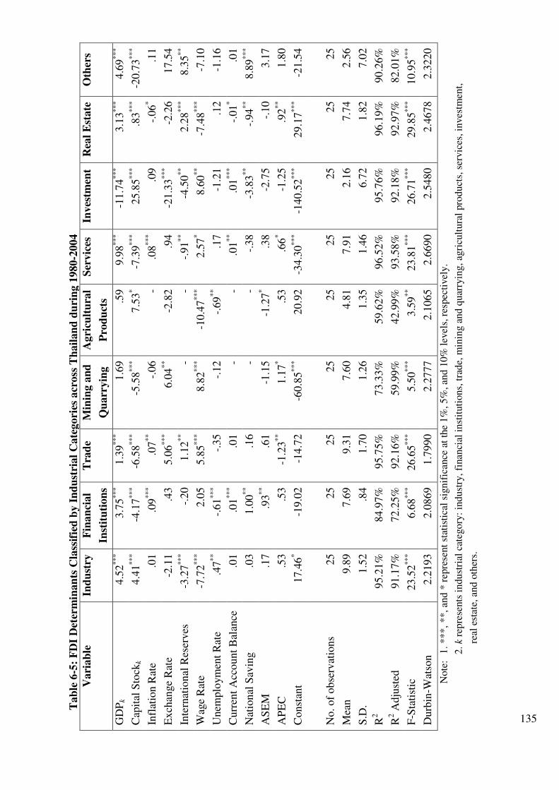
135
Tab
le 6
-5:
FD
I D
eter
min
an
ts C
lass
ifie
d b
y I
nd
ust
rial
Cate
gori
es a
cross
Th
ail
an
d d
uri
ng 1
980-2
004
V
ari
ab
le
Ind
ust
ry
Fin
an
cial
Inst
itu
tion
s
Tra
de
Min
ing a
nd
Qu
arr
yin
g
Agri
cult
ura
l
Pro
du
cts
Ser
vic
es
Inves
tmen
t R
eal
Est
ate
O
ther
s
GD
Pk
4.5
2***
3.7
5***
1.3
9***
1.6
9
.59
9.9
8***
-11.7
4***
3.1
3***
4.6
9***
Cap
ital
Sto
ckk
4.4
1***
-4.1
7***
-6.5
8***
-5.5
8***
7.5
3*
-7.3
9***
25.8
5***
.83
***
-20.7
3***
Infl
atio
n R
ate
.01
.09
***
.07
**
-.06
- .0
8***
.09
-.06
*
.11
Ex
chan
ge
Rat
e -2
.11
.43
5.0
6***
6.0
4**
-2.8
2
.94
-21.3
3***
-2.2
6
17.5
4
Inte
rnat
ional
Res
erves
-3
.27
***
-.20
1.1
2**
- -
-.91
**
-4.5
0**
2.2
8***
8.3
5**
Wag
e R
ate
-7.7
2***
2.0
5
5.8
5***
8.8
2***
-10.4
7***
2.5
7*
8.6
0**
-7.4
8***
-7.1
0
Unem
plo
ym
ent
Rat
e .4
7**
-.61
***
-.35
-.12
-.69
**
.17
-1.2
1
.12
-1.1
6
Curr
ent
Acc
ount
Bal
ance
.0
1
.01
***
.01
- -
.01
**
.01
***
-.01
*
.01
Nat
ional
Sav
ing
.03
1.0
0**
.16
- -
-.38
-3.8
3**
-.94
**
8.8
9***
AS
EM
.1
7
.93
**
.61
-1.1
5
-1.2
7*
.38
-2.7
5
-.10
3.1
7
AP
EC
.5
3
.53
-1.2
3**
1.1
7*
.53
.66
*
-1.2
5
.92
**
1.8
0
Const
ant
17.4
6*
-19.0
2
-14.7
2
-60.8
5***
20.9
2
-34.3
0***
-140.5
2***
29.1
7***
-21.5
4
No. of
obse
rvat
ions
25
25
25
25
25
25
25
25
25
Mea
n
9.8
9
7.6
9
9.3
1
7.6
0
4.8
1
7.9
1
2.1
6
7.7
4
2.5
6
S.D
. 1.5
2
.84
1.7
0
1.2
6
1.3
5
1.4
6
6.7
2
1.8
2
7.0
2
R2
95.2
1%
84.9
7%
95.7
5%
73.3
3%
59.6
2%
96.5
2%
95.7
6%
96.1
9%
90.2
6%
R2 A
dju
sted
91.1
7%
72.2
5%
92.1
6%
59.9
9%
42.9
9%
93.5
8%
92.1
8%
92.9
7%
82.0
1%
F-S
tati
stic
23.5
2***
6.6
8***
26.6
5***
5.5
0***
3.5
9**
23.8
1***
26.7
1***
29.8
5***
10.9
5***
Durb
in-W
atso
n
2.2
193
2.0
869
1.7
990
2.2
777
2.1
065
2.6
690
2.5
480
2.4
678
2.3
220
Note
: 1
. ***, **, an
d *
rep
rese
nt
stat
isti
cal
signif
ican
ce a
t th
e 1%
, 5%
, an
d 1
0%
lev
els,
res
pec
tivel
y.
2. k
repre
sents
indust
rial
cat
egory
: in
dust
ry, fi
nan
cial
inst
ituti
ons,
tra
de,
min
ing a
nd q
uar
ryin
g, ag
ricu
ltura
l pro
duct
s, s
ervic
es, in
ves
tmen
t,
r
eal
esta
te, an
d o
ther
s.
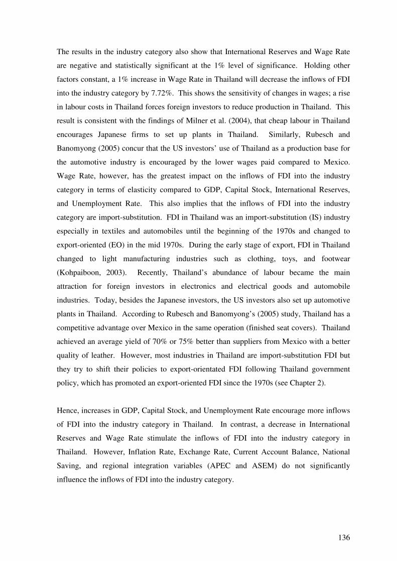
136
The results in the industry category also show that International Reserves and Wage Rate
are negative and statistically significant at the 1% level of significance. Holding other
factors constant, a 1% increase in Wage Rate in Thailand will decrease the inflows of FDI
into the industry category by 7.72%. This shows the sensitivity of changes in wages; a rise
in labour costs in Thailand forces foreign investors to reduce production in Thailand. This
result is consistent with the findings of Milner et al. (2004), that cheap labour in Thailand
encourages Japanese firms to set up plants in Thailand. Similarly, Rubesch and
Banomyong (2005) concur that the US investors’ use of Thailand as a production base for
the automotive industry is encouraged by the lower wages paid compared to Mexico.
Wage Rate, however, has the greatest impact on the inflows of FDI into the industry
category in terms of elasticity compared to GDP, Capital Stock, International Reserves,
and Unemployment Rate. This also implies that the inflows of FDI into the industry
category are import-substitution. FDI in Thailand was an import-substitution (IS) industry
especially in textiles and automobiles until the beginning of the 1970s and changed to
export-oriented (EO) in the mid 1970s. During the early stage of export, FDI in Thailand
changed to light manufacturing industries such as clothing, toys, and footwear
(Kohpaiboon, 2003). Recently, Thailand’s abundance of labour became the main
attraction for foreign investors in electronics and electrical goods and automobile
industries. Today, besides the Japanese investors, the US investors also set up automotive
plants in Thailand. According to Rubesch and Banomyong’s (2005) study, Thailand has a
competitive advantage over Mexico in the same operation (finished seat covers). Thailand
achieved an average yield of 70% or 75% better than suppliers from Mexico with a better
quality of leather. However, most industries in Thailand are import-substitution FDI but
they try to shift their policies to export-orientated FDI following Thailand government
policy, which has promoted an export-oriented FDI since the 1970s (see Chapter 2).
Hence, increases in GDP, Capital Stock, and Unemployment Rate encourage more inflows
of FDI into the industry category in Thailand. In contrast, a decrease in International
Reserves and Wage Rate stimulate the inflows of FDI into the industry category in
Thailand. However, Inflation Rate, Exchange Rate, Current Account Balance, National
Saving, and regional integration variables (APEC and ASEM) do not significantly
influence the inflows of FDI into the industry category.
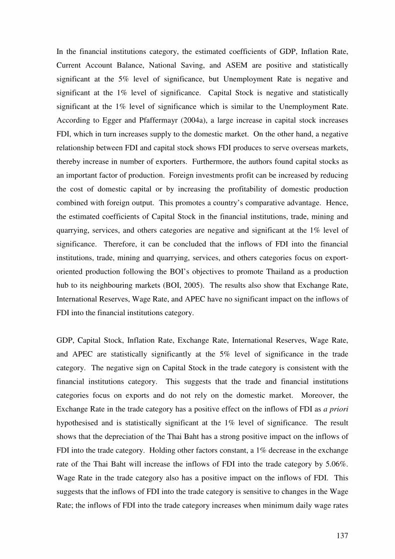
137
In the financial institutions category, the estimated coefficients of GDP, Inflation Rate,
Current Account Balance, National Saving, and ASEM are positive and statistically
significant at the 5% level of significance, but Unemployment Rate is negative and
significant at the 1% level of significance. Capital Stock is negative and statistically
significant at the 1% level of significance which is similar to the Unemployment Rate.
According to Egger and Pfaffermayr (2004a), a large increase in capital stock increases
FDI, which in turn increases supply to the domestic market. On the other hand, a negative
relationship between FDI and capital stock shows FDI produces to serve overseas markets,
thereby increase in number of exporters. Furthermore, the authors found capital stocks as
an important factor of production. Foreign investments profit can be increased by reducing
the cost of domestic capital or by increasing the profitability of domestic production
combined with foreign output. This promotes a country’s comparative advantage. Hence,
the estimated coefficients of Capital Stock in the financial institutions, trade, mining and
quarrying, services, and others categories are negative and significant at the 1% level of
significance. Therefore, it can be concluded that the inflows of FDI into the financial
institutions, trade, mining and quarrying, services, and others categories focus on export-
oriented production following the BOI’s objectives to promote Thailand as a production
hub to its neighbouring markets (BOI, 2005). The results also show that Exchange Rate,
International Reserves, Wage Rate, and APEC have no significant impact on the inflows of
FDI into the financial institutions category.
GDP, Capital Stock, Inflation Rate, Exchange Rate, International Reserves, Wage Rate,
and APEC are statistically significantly at the 5% level of significance in the trade
category. The negative sign on Capital Stock in the trade category is consistent with the
financial institutions category. This suggests that the trade and financial institutions
categories focus on exports and do not rely on the domestic market. Moreover, the
Exchange Rate in the trade category has a positive effect on the inflows of FDI as a priori
hypothesised and is statistically significant at the 1% level of significance. The result
shows that the depreciation of the Thai Baht has a strong positive impact on the inflows of
FDI into the trade category. Holding other factors constant, a 1% decrease in the exchange
rate of the Thai Baht will increase the inflows of FDI into the trade category by 5.06%.
Wage Rate in the trade category also has a positive impact on the inflows of FDI. This
suggests that the inflows of FDI into the trade category is sensitive to changes in the Wage
Rate; the inflows of FDI into the trade category increases when minimum daily wage rates
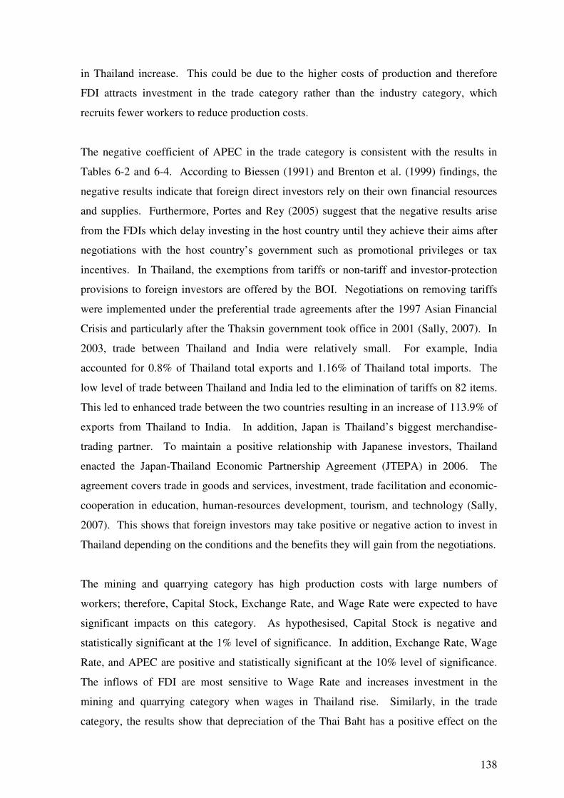
138
in Thailand increase. This could be due to the higher costs of production and therefore
FDI attracts investment in the trade category rather than the industry category, which
recruits fewer workers to reduce production costs.
The negative coefficient of APEC in the trade category is consistent with the results in
Tables 6-2 and 6-4. According to Biessen (1991) and Brenton et al. (1999) findings, the
negative results indicate that foreign direct investors rely on their own financial resources
and supplies. Furthermore, Portes and Rey (2005) suggest that the negative results arise
from the FDIs which delay investing in the host country until they achieve their aims after
negotiations with the host country’s government such as promotional privileges or tax
incentives. In Thailand, the exemptions from tariffs or non-tariff and investor-protection
provisions to foreign investors are offered by the BOI. Negotiations on removing tariffs
were implemented under the preferential trade agreements after the 1997 Asian Financial
Crisis and particularly after the Thaksin government took office in 2001 (Sally, 2007). In
2003, trade between Thailand and India were relatively small. For example, India
accounted for 0.8% of Thailand total exports and 1.16% of Thailand total imports. The
low level of trade between Thailand and India led to the elimination of tariffs on 82 items.
This led to enhanced trade between the two countries resulting in an increase of 113.9% of
exports from Thailand to India. In addition, Japan is Thailand’s biggest merchandise-
trading partner. To maintain a positive relationship with Japanese investors, Thailand
enacted the Japan-Thailand Economic Partnership Agreement (JTEPA) in 2006. The
agreement covers trade in goods and services, investment, trade facilitation and economic-
cooperation in education, human-resources development, tourism, and technology (Sally,
2007). This shows that foreign investors may take positive or negative action to invest in
Thailand depending on the conditions and the benefits they will gain from the negotiations.
The mining and quarrying category has high production costs with large numbers of
workers; therefore, Capital Stock, Exchange Rate, and Wage Rate were expected to have
significant impacts on this category. As hypothesised, Capital Stock is negative and
statistically significant at the 1% level of significance. In addition, Exchange Rate, Wage
Rate, and APEC are positive and statistically significant at the 10% level of significance.
The inflows of FDI are most sensitive to Wage Rate and increases investment in the
mining and quarrying category when wages in Thailand rise. Similarly, in the trade
category, the results show that depreciation of the Thai Baht has a positive effect on the

139
inflows of FDI into the mining and quarrying category. The Exchange Rate is important in
determining FDI in the mining and quarrying category due to the costs of labour. The FDI
in the mining and quarrying category needs to hire skilled labour, which is more expensive
than unskilled labour. This increases the cost of production to the FDI. To reduce the
production cost, the FDI prefers a depreciation of the Thai Baht which decreases the
production costs in Thailand and increases profits from the low prices for exports to the
global market. Thus FDI is sensitive to the Exchange Rate changes. The coefficient of
APEC is positive and statistically significant at the 10% level of significance. This occurs
for three reasons. First, the result implies that FDIs invest in APEC member countries to
export to APEC members’ markets through improved market access (Elek, 1992). Second,
FDIs can improve Thailand’s domestic markets in Thailand with their investment
resources, such as offering skill training programmes, transferring useful know-how,
enhancing job opportunities, and improving national revenues. In addition, FDIs with their
technology and advanced R&D are able to use the natural resources more efficiently
compared to domestic investors. Third, FDIs gain advantages from trade exemptions such
as the elimination of tariff or non-tariff under the APEC agreement amongst members.
Therefore, most FDIs in this category come from APEC members such as the US or Japan.
Thailand is an agricultural-based country with up to 40% of the total labour force involved
in agriculture in 2003 (BOT, 2004). However, foreign investors have never focused on
this category as shown by the small number of applications for promotional privileges
from the BOI. For example, 0.5% of the total FDI received promotional privileges from
BOI during 1980-2004 (see Table 2-3). There may be two reasons for this. First,
agricultural-based industrial production has never attracted investors due to the unreliable
price of agricultural products in the global market and the high risk of unpredictable and
uncontrollable factors such as weather. Second, it may be because the Thai government
has set up a policy to control price and quantity in some agricultural products such as rice
and sugar to export to the global market. If the investors would like to export, they need
government authorisation before exporting to importers under the government list. In
Thailand, there are very few successes in agriculture that are not involved with or
subsidised by the government. For example, Thailand used the Rice Office to keep the
price of rice as low as politically possible (Rock, 2002). The price of rice in Thailand is
guaranteed by the Thai government to be as low and stable. In addition, the government
intervenes by implementing a variety of taxes on the price of rice that increase when there
140
is a shortage of rice in the markets, and decrease when there is an excess of rice supply.
Table 6-5 shows Capital Stock on the inflows of FDI into the agricultural products
category is positive and statistically significant at the 10% level of significance. The Wage
Rate, Unemployment Rate, and ASEM are negative and statistically significant at the 10%
level of significance. A negative and significant Wage Rate variable in the agricultural
products category indicates that the inflows of FDI are greater in locations with relatively
low labour costs. This result suggests that Wage Rate has the greatest impact on the
inflows of FDI in terms of elasticity compared to other categories. Holding other factors
constant, a 1% increase in the Wage Rate in Thailand will decrease the inflows of FDI into
the agricultural products category by 10.47%. Even the FDI in the agricultural products
category does not produce goods to export, but wage rate is one of the production costs. If
the cost is high then the price will be raised and cannot compete in the domestic market. In
addition, the positive coefficient sign on Capital Stock in the agricultural products category
suggests that foreign investors prefer to invest in agricultural products in Thailand to serve
the domestic market rather than for export. GDP, Exchange Rate, and APEC have no
impact on the inflows of FDI in the agricultural products category (see Table 6-5).
The services category shows that GDP and Inflation Rate are positive and statistically
significant at the 1% level of significance (see Table 6-5). In addition, the Current
Account Balance is positive and statistically significant at the 5% level of significance and
Wage Rate and APEC are positive and statistically significant at the 10% level of
significance. The results in the services category demonstrate that GDP is the most
important factor for inflow of FDI in terms of elasticity. The GDP elasticity on the inflows
of FDI in the services category is 9.98 compared to Capital Stock (-7.39), Inflation Rate
(0.08), International Reserves (-.91), Wage Rate (2.57), Current Account Balance (.01),
and APEC (.66). The Capital Stock coefficient is negative and statistically significant at
the 1% level of significance. This is consistent with Egger and Pfaffermayr’s (2004a)
findings that the negative sign on Capital Stock reveals an export-oriented strategy for FDI
and it is an important factor in production that fosters a country’s comparative advantage.
This suggests that the inflows of FDI into the services category are serving the external
markets. Sally (2007) also reports that the FDI from the US is the main investor to invest
in the services category in Thailand. The FDIs from the US are making very ambitious
demands in negotiations and investment in this category since Thailand announced the
Master plan for Telecommunications Development in 1997 to arrange the liberalisation of
141
basic telecommunications services by 2006 (Sally, 1999). This increased the inflows of
FDI in the services category from less than 3% of the total of FDI per year to 7% and 12%
in 1997 and 2002, respectively (see Table 2-3). Moreover, the Thai government has
attracted more inward FDI by improving transportation and infrastructure systems under
the Eastern Seaboard Programme to build a new deep sea port, rail way, and cargo airport
in the Eastern part of Thailand in the 1990s. This may attract more inflows of FDI into the
services category, more than in the late 1990s to the 2000s, which allow foreign investors
to fully own buildings and land in the industrial estate. This estate provides advanced
technologies and superior infrastructure to foreign investors to service or ship overseas.
The coefficient of APEC in the services category is positive and statistically significant at
the 10% level of significance. This is related to the fact that most foreign investors in this
category come from the US, which is a member of APEC, as is Thailand. Therefore, the
US takes advantage of the APEC membership by investing in Thailand. The Exchange
Rate, Unemployment Rate, National Saving, and ASEM do not have a significant effect on
the inflows of FDI into the services category.
In the investment category, GDP, Exchange Rate, International Reserves, and National
Saving are negative, but Capital Stock, Wage Rate, and Current Account Balance are
positive and statistically significantly at the 5% level of significance. The inflows of FDI
into the investment category are sensitive to changes in Capital Stock followed by
Exchange Rate. For example, a 1% increase in Capital Stock in the investment category
will increase the inflows of FDI by 25.85%, and a 1% depreciation of the exchange rate
decreases the inflows of FDI into the investment category by 21.33% (see Table 6-5). The
results suggest that foreign investors investing in the investment category in Thailand
focused on the domestic market. Therefore, FDIs prefer a strong Thai Baht, which reflects
the strength of the Thai economy and the increase in demands and purchasing powers of
consumers in Thailand. Moreover, Wage Rate has a positive and significant effect on the
inflows of FDI into the investment category. A higher wage rate shows a higher income
and implies higher welfare and higher power purchasing power for consumers in the
domestic market. When the quality of life in Thailand increases, the inflows of FDI may
focus on investing in the investment category rather than other categories. However, the
total of the inflows of FDI into the investment category is very small and its total value has
not been greater than US$ 1 million since 1992 (see Table 2-3). Inflation Rate and the
142
regional integration dummy variables (APEC and ASEM) appear to have no significant
effect on the inflows of FDI into the investment category.
The value of the inflows of FDI into the real estate category was very high before the 1997
Asian Financial Crisis. For example, Table 2-3 shows that the inflows of FDI in the real
estate category was 8.27% in 1992 and increased to 28.54% the following year and
remained at this rate until 1996 before decreasing to 2.25% in 1997 and 0.41% in 1998
(BOI, 2005; BOT, 2005). The results show GDP, Capital Stock, International Reserves,
and APEC are positive and statistically significant at the 5% or lower level of significance.
On the other hand, the coefficients of Inflation Rate, Wage Rate, Current Account Balance,
and National Saving are negative and statistically significantly at the 10% level of
significance. Wage Rate is found to be the most important factor in determining the
inflows of FDI with an elasticity of -7.48. Holding other factors constant, a 1% increase in
labour wage in Thailand will decrease the inflows of FDI into the real estate category by
7.48%. This may be due to high demands and the numbers of workers required to build
the buildings. Most foreign investors who invest in the real estate category in Thailand
focused on foreign customers. The foreign investors prefer a short-term investment to a
long-term investment in order to earn higher revenue and avoid the possibility of economic
unpredictability such as exchange rate volatility and political changes. Most foreign
investors in this category are from Hong Kong, Singapore, and Taiwan (see Appendix A).
These foreign investors represent highly influential participants in the real estate category.
However, after the 1997 Asian Financial Crisis, the number of the inflows of FDI into the
real estate category reduced dramatically to 0.41% in 1998 and remained less than 2% of
the total of the inflows of FDI in the following years.
The results for the inflows of FDI into the others category show that GDP, Capital Stock,
International Reserves, and National Saving are important in determining the inflows of
FDI into Thailand. Inflation Rate, Exchange Rate, Wage Rate, Unemployment Rate,
Current Account Balance, ASEM, and APEC do not influence FDI in the others category.
Table 6-5 shows that the inflows of FDI into nine industrial categories: industry, financial
institutions, trade, mining and quarrying, agricultural products, services, investment, real
estate, and others, are sensitive to changes in Capital Stock. Capital Stock has the greatest
impact on the inflows of FDI into the investment category compared to other categories
143
with an elasticity of 25.85. GDP has a positive and significant impact on all categories
except on the mining and quarrying and the agricultural products categories but is negative
in the investment category. The financial institutions category is not sensitive to wages,
while Wage Rate has a negative impact on the inflows of FDI into the industry, agricultural
products, and real estate categories. The rise in labour wages in Thailand would cause the
inflows of FDI to decline. However, Wage Rate has a positive impact on the inflows of
FDI into the trade, mining and quarrying, services and investment categories. Only three
categories, trade, mining and quarrying, and investment, are impacted by the Exchange
Rate. When FDI is export-oriented, the Exchange Rate is found to be positive and
significant, such as in the trade and mining and quarrying categories. On the other hand,
the Exchange Rate has a negative impact on import-substitution FDI such as FDI in the
investment category. Only the inflows of FDI into the financial institutions category are
not impacted by International Reserves. The numbers of workers and unemployment rate
have significant impacts on the inflows of FDI into the industry, financial institutions, and
agricultural products categories. Inflation Rate, Current Account Balance, and National
Saving have no significant impact on the inflows of FDI into some categories such as the
industry and mining and quarrying. However, the financial institutions, trade, mining and
quarrying, services, and others categories are promoted as export-oriented production by
the Thai government. The strategy of the inflows of FDI into this group takes advantage of
the abundance of labour and lower wages in Thailand in order to reduce production costs.
This is considered an efficiency-seeking FDI, whereas the inflows of FDI into the industry,
agricultural products, investment, and real estate categories complement the import-
substitution FDI focusing on the domestic market. Even some industries in Thailand are
promoted to be export-oriented such as electronics/electrical products and textile, but the
overall image of the industry category is one of import-substitution.
From the results, it can be concluded that the financial institutions, trade, mining and
quarrying, services, and others categories are vertical FDI and the others are horizontal
FDI. In integration networks, FDI in Thailand may offer attractive operating
environments for export-oriented FDI in an efficiency-seeking strategy: low wage rates
and the number of workers. Thus, FDI builds production networks in Thailand in response
to such factors to gain overall efficiency. Import-substitution FDI is determined by market
size, growth and attractiveness of the domestic market (Thai economy), such as GDP and
capital stock and the investment climate. Import-substitution FDI does not enter into
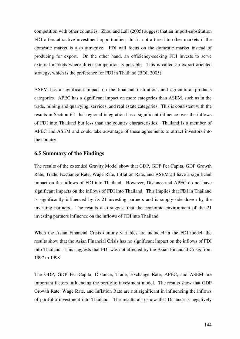
144
competition with other countries. Zhou and Lall (2005) suggest that an import-substitution
FDI offers attractive investment opportunities; this is not a threat to other markets if the
domestic market is also attractive. FDI will focus on the domestic market instead of
producing for export. On the other hand, an efficiency-seeking FDI invests to serve
external markets where direct competition is possible. This is called an export-oriented
strategy, which is the preference for FDI in Thailand (BOI, 2005)
ASEM has a significant impact on the financial institutions and agricultural products
categories. APEC has a significant impact on more categories than ASEM, such as in the
trade, mining and quarrying, services, and real estate categories. This is consistent with the
results in Section 6.1 that regional integration has a significant influence over the inflows
of FDI into Thailand but less than the country characteristics. Thailand is a member of
APEC and ASEM and could take advantage of these agreements to attract investors into
the country.
6.5 Summary of the Findings
The results of the extended Gravity Model show that GDP, GDP Per Capita, GDP Growth
Rate, Trade, Exchange Rate, Wage Rate, Inflation Rate, and ASEM all have a significant
impact on the inflows of FDI into Thailand. However, Distance and APEC do not have
significant impacts on the inflows of FDI into Thailand. This implies that FDI in Thailand
is significantly influenced by its 21 investing partners and is supply-side driven by the
investing partners. The results also suggest that the economic environment of the 21
investing partners influence on the inflows of FDI into Thailand.
When the Asian Financial Crisis dummy variables are included in the FDI model, the
results show that the Asian Financial Crisis has no significant impact on the inflows of FDI
into Thailand. This suggests that FDI was not affected by the Asian Financial Crisis from
1997 to 1998.
The GDP, GDP Per Capita, Distance, Trade, Exchange Rate, APEC, and ASEM are
important factors influencing the portfolio investment model. The results show that GDP
Growth Rate, Wage Rate, and Inflation Rate are not significant in influencing the inflows
of portfolio investment into Thailand. The results also show that Distance is negatively
145
and significantly related to the size of portfolio investments. This indicates that
information costs have a greater influence on portfolio investment than on the FDI model.
APEC and ASEM negatively affect the determinants of portfolio investment in Thailand,
while APEC and ASEM have positive impacts on the FDI model. This means foreign
investors readily shift their funds to Thailand’s capital markets immediately after they
receive their negotiated exemption incentives from the Thai government. The results also
suggest that the inflows of portfolio investment into Thailand are mainly driven by the
Thai economy and are not influenced by the economic status of the 21 investing partners.
The Asian Financial Crisis dummy variables positively impact the inflows of portfolio
investment into Thailand during 1997-1998. The results indicate that the Asian Financial
Crisis in mid-1997 increased total foreign portfolio investment in Thailand. The results
suggest that the activity of foreign portfolio investors is different from the activity of
foreign direct investors. The inflows of FDI into Thailand were more stable than the other
form (such as portfolio investment) of foreign investment flows during the 1997 Asian
Financial Crisis. This indicates that portfolio investment in Thailand does not follow the
FDI pattern.
In terms of industrial category, the results suggest that the inflows of FDI into Thailand are
both an export-oriented investment and import-substitution investment, which is both a
market-seeking and efficiency-seeking FDI respectively. The export-oriented FDI are in
the financial institutions, trade, mining and quarrying, services, and others categories. The
industry, agricultural products, investment, and real estate categories act as import-
substitution FDI in Thailand.
The results show that Capital Stock is an important factor for all the FDI categories:
industry, financial institutions, trade, mining and quarrying, agricultural products, services,
investment, real estate, and others. However, in the case of investment and others
categories, the Capital Stock is found to have a greater impact on the inflows of FDI in
terms of elasticity. The Exchange Rate has positive effects on an export-oriented FDI but
negative effects on an import-substitution FDI. However, only three categories: trade,
mining and quarrying, and investment, are affected by Exchange Rate. For the industry,
agricultural products, real estate, and others categories, Wage Rate has a negative impact
when the amount of labour wage is decreased with an increase in the total of the inflows of
146
FDI in these categories. In the industry, financial institutions, and agricultural products
categories, Unemployment Rate has a significant impact on the inflows of FDI. The
Current Account Balance has a positive effect on all industrial categories but a significant
impact on the financial institutions, services, investment, and real estate categories. The
Inflation Rate has a negative impact on the real estate category, which is an import-
substitution FDI, but a positive impact on the financial institutions, trade, and services
categories, which are export-oriented FDI. ASEM has a significant impact on the financial
institutions and agricultural propducts categories. APEC has a significant impact on the
trade, mining and quarrying, services, and real estate categories. This shows that the
regional integration has a significant influence on the inflows of FDI into Thailand.

CHAPTER 7
CONCLUSIONS AND IMPLICATIONS This chapter presents a summary of the study, including the empirical results and the study
issues that emerged. Section 7.1 discusses the conclusions drawn from the empirical
models. Section 7.2 discusses the policy implications of the research findings. Section 7.3
identifies the limitations of the study. Section 7.4 discusses the contribution of the thesis
results and findings and Section 7.5 provides suggestions for future research.
7.1 Summary and Empirical Findings
Thailand has been a significant recipient of FDI among developing countries over the last
30 years, and has recorded rapid and sustained growth rates in a number of different
industrial categories. Thailand has shown a clear policy transition for foreign investment
over time from an import-substitution regime to an export-oriented regime. Before the
1997 Asian Financial Crisis (1985-1996), Thailand had the fastest growing level of exports
in manufactured goods among Asian economies. Therefore, FDI plays a significant role in
the Thai economy. Thailand has been pursuing different foreign investment policies at
different times depending on the development objectives and economic situation in the
country. Thus, an understanding of the determinants of FDI is an important element for
motivating and attracting more FDI into Thailand. In addition, it is important for the Thai
government to promote and develop programmes to attract FDI into Thailand.
The objectives of this study are to compare and contrast the Eclectic Paradigm, Resourced-
Based Theory, and Business Network Theory concepts relating to the determinants of FDI;
to evaluate the determinants of FDI and foreign portfolio investment flows into Thailand;
and to study the effects of the 1997 Asian Financial Crisis on the pattern of FDI and
foreign portfolio investment inflows in Thailand. In addition, this study also investigates
the relationship of FDI inflow, as classified by industrial category in Thailand.
The literature on Eclectic Paradigm, Resourced-based Theory, and Business Network
Theory is reviewed thoroughly in Chapter 3. The Eclectic Paradigm provides the
analytical basis for an international production and foreign investments. Its concept is
148
based on three factors: ownership, location, and internalisation. This is expected to assist
researchers and businesses to identify the nature of FDI through global competitiveness; to
investigate the effects of FDI on the host country and its competitive advantages; to
develop the FDI policies for governments (host and home countries); to sustain economic
prosperity; and to respond to the changes to competitive conditions in the industrial
sectors.
The Resource-Based Theory explains the knowledge and performance indicators in the
FDI model. The theory is applied at the firm-level, which possesses resources and
capabilities such as financial, physical, human, and organisational resources. FDI develops
the Resource-Based Theory as an effective strategy to achieve sustainable competitive
advantages and to develop its capabilities and resources to attain a better performance.
The Resource-Based Theory suggests FDI successfully makes the transition from resource-
based industries to high technology industries.
The Business Network Theory in FDI maintains the relationships between firms such as
strategic alliances, joint ventures, and buyer-supplier partnerships. This theory has
promoted the framework of relationships between firms or countries for FDI to analyse the
resources in foreign markets and to sustain the competitive advantage (i.e., technological
know-how and management expertise). FDI gains economies of scale and scope, improves
operational efficiency, reduces numbers of competitors and barriers, and increases growth
over the long term.
To answer to research objectives two and three, an extended form of the Gravity Model
derived from the conventional Gravity Model is utilised to examine the determinants of
FDI and portfolio flows in Thailand with the panel data covering the time period of 1980-
2004 and 21 major investing partners. In addition, this study has investigated the impact of
the 1997 Asian Financial Crisis on FDI and portfolio investment in Thailand.
The explanatory variables in the FDI and portfolio investment models include GDP, GDP
Per Capita, GDP Growth Rate, Distance, Trade, Exchange Rate, Wage Rate, Inflation
Rate, regional integration dummy variables (APEC and ASEM), and the Asian Financial
Crisis dummy variables (1997 and 1998). The regression results support the claim that the
extended Gravity Model specification can be used to determine the inflows of FDI and
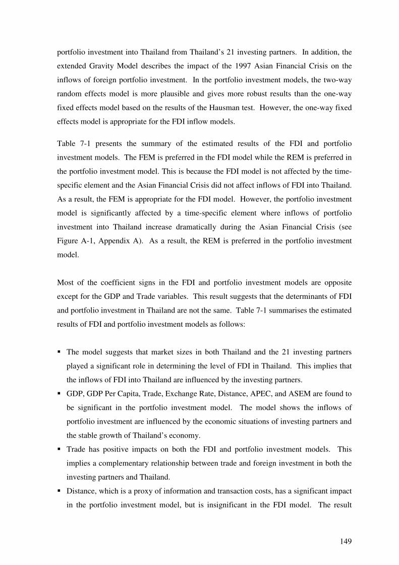
149
portfolio investment into Thailand from Thailand’s 21 investing partners. In addition, the
extended Gravity Model describes the impact of the 1997 Asian Financial Crisis on the
inflows of foreign portfolio investment. In the portfolio investment models, the two-way
random effects model is more plausible and gives more robust results than the one-way
fixed effects model based on the results of the Hausman test. However, the one-way fixed
effects model is appropriate for the FDI inflow models.
Table 7-1 presents the summary of the estimated results of the FDI and portfolio
investment models. The FEM is preferred in the FDI model while the REM is preferred in
the portfolio investment model. This is because the FDI model is not affected by the time-
specific element and the Asian Financial Crisis did not affect inflows of FDI into Thailand.
As a result, the FEM is appropriate for the FDI model. However, the portfolio investment
model is significantly affected by a time-specific element where inflows of portfolio
investment into Thailand increase dramatically during the Asian Financial Crisis (see
Figure A-1, Appendix A). As a result, the REM is preferred in the portfolio investment
model.
Most of the coefficient signs in the FDI and portfolio investment models are opposite
except for the GDP and Trade variables. This result suggests that the determinants of FDI
and portfolio investment in Thailand are not the same. Table 7-1 summarises the estimated
results of FDI and portfolio investment models as follows:
� The model suggests that market sizes in both Thailand and the 21 investing partners
played a significant role in determining the level of FDI in Thailand. This implies that
the inflows of FDI into Thailand are influenced by the investing partners.
� GDP, GDP Per Capita, Trade, Exchange Rate, Distance, APEC, and ASEM are found to
be significant in the portfolio investment model. The model shows the inflows of
portfolio investment are influenced by the economic situations of investing partners and
the stable growth of Thailand’s economy.
� Trade has positive impacts on both the FDI and portfolio investment models. This
implies a complementary relationship between trade and foreign investment in both the
investing partners and Thailand.
� Distance, which is a proxy of information and transaction costs, has a significant impact
in the portfolio investment model, but is insignificant in the FDI model. The result
150
indicates that a decrease in information and transaction costs will increase the inflows of
foreign portfolio investment into Thailand. This shows that distance impacts the FDI
and portfolio investment models differently.
Table 7-1: Variables Affecting the Determinants of FDI and Portfolio Investment in Thailand
Variables FDI Portfolio Investment
GDP (+) (+)
GDP Per Capita (-) (+)
GDP Growth Rate (+) (0)
Distance (0) (-)
Trade (+) (+)
Exchange Rate (-) (+)
Wage Rate (+) (0)
Inflation Rate (+) (0)
APEC (0) (-)
ASEM (+) (-)
1997 (0) (+)
1998 (0) (+)
FEM REM
Note: 1. (+), (-) and (0) represent positive, negative, and no significant effect, respectively.
2. FEM and REM represent fixed and random effects model, respectively. 3. The summary of FDI model is based on Model 4 (see Table 6-3).
4. The summary of portfolio investment model is based on Model 4 (see Table 6-4).
151
� The exchange rate in the orthodox context of the Gravity Model is expected to produce
either positive or negative effects depending on export/import or inflow/outflow of
investment (Cortes Rodriguez, 2002; Dascal et al., 2002). For example, the
appreciation of a country’s currency against other currencies reduces the countries’
exports (in terms of trade) and/or inflows of FDI, and depreciation of the currency
stimulates the country’s exports and/or inflows of FDI (Bersgtrand, 1985; 1989). In this
study, the exchange rates in FDI and portfolio investment models yield an opposite sign.
As shown in the FDI model, the inflows of FDI have been negatively affected by the
exchange rate due to the appreciation of the Thai Baht, therefore, investors import parts,
components, and raw materials for their production processes in Thailand. This
suggests that FDI relies on overseas parts, to be available for production to commence.
Thus, an appreciation of Thai Baht raises the inflows of FDI into Thailand. In contrast,
exchange rate has a positive impact on the inflows of foreign portfolio investment. The
results show that a depreciation of the Thai Baht tends to increase foreign portfolio
investment in Thailand.
� The variables capturing the investing partners’ economies such as GDP growth rate,
wage rate, and inflation rate are significantly and positively related to FDI. This implies
that the inflows of FDI into Thailand are driven by the economic status of the investing
partners. The state of the investing partners’ economies can be understood to stimulate
much of the inflows of FDI into Thailand. Furthermore, the results show that the
investing partners with stronger economies tend to invest in larger amounts.
� ASEM has a positive and a negative influence on FDI and portfolio investment models,
respectively. However, APEC has no impact on the FDI model but it has a negative
impact on the portfolio investment model. In addition, it should be noted that most of
the regional integration dummy variables are negatively related to the FDI and portfolio
investment in Thailand. This indicates the existence of delays in the inflows of foreign
funds into Thailand until the Thai government offers promotional privileges demanded
by the foreign investors. This indirectly shows the co-operation of Thailand’s investing
partners have an influence on government policies in Thailand. In addition, foreign
investors will invest in Thailand if the perceived profitability of their capital is secured
with protection from the Thai government.
� The portfolio investment model shows that the Asian Financial Crisis had a strong
influence on foreign investment decisions. The Asian Financial Crisis dummy variables
show positive impacts on the portfolio investment model in 1997 and 1998. However,
152
the crisis has no impact on the FDI model. This shows the importance of a healthy and
stable economy in Thailand to attract and sustain the inflows of foreign portfolio
investment into the country.
� FDI inflows into Thailand during 1980-2004 are supply-side driven by the investing
partners’ economies. In contrast, the portfolio investment in Thailand during the same
period is driven by both Thai and the investing partners’ economic situations.
The determinants of the inflows of FDI in nine different industrial categories in Thailand
during 1980-2004 are summarized as follows (see Table 7-2):
� The results suggest that the industry, agricultural products, investment, and real estate
categories are promoted as import-substitution FDI. On the other hand, the financial
institutions, trade, mining and quarrying, services, and others categories are promoted as
export-oriented FDI.
� Exchange rate is an important determinant of the inflows of FDI in different industrial
categories. Exchange rate has a negative impact on import-substitution FDI, but a
positive impact on export-oriented FDI. The negative impact on import-substitution
FDI indicates that import-substitution FDI focuses on production to cater to the
domestic market rather than external markets. In contrast, the positive impact on
export-oriented FDI suggests that FDI takes advantage of the low price of goods in the
global market generated from the depreciation of the Thai Baht.
� Capital stock has a positive impact on import-substitution FDI, but a negative impact on
export-oriented FDI. This shows that foreign investors in the industry, agricultural
products, investment, and real estate categories are influenced by the numbers of capital
stocks in Thailand, such as land, building, and fixed assets.
� Inflation rate in Thailand has no impact on the inflows of import-substitution FDI, with
the exception of the real estate category. Inflation rate affects exchange rates
negatively. For example, inflation rate negatively impacts foreign investors who wish
to transfer profits back to their countries. Conversely, the risk of exchange rate changes
does not significantly influence import-substitution FDI. This may be because foreign
investors only wish to supply their products to Thailand and reinvest their production in
Thailand. Export-oriented FDI such as the financial institutions, trade, and services
categories, are strongly influenced by the inflation rate.
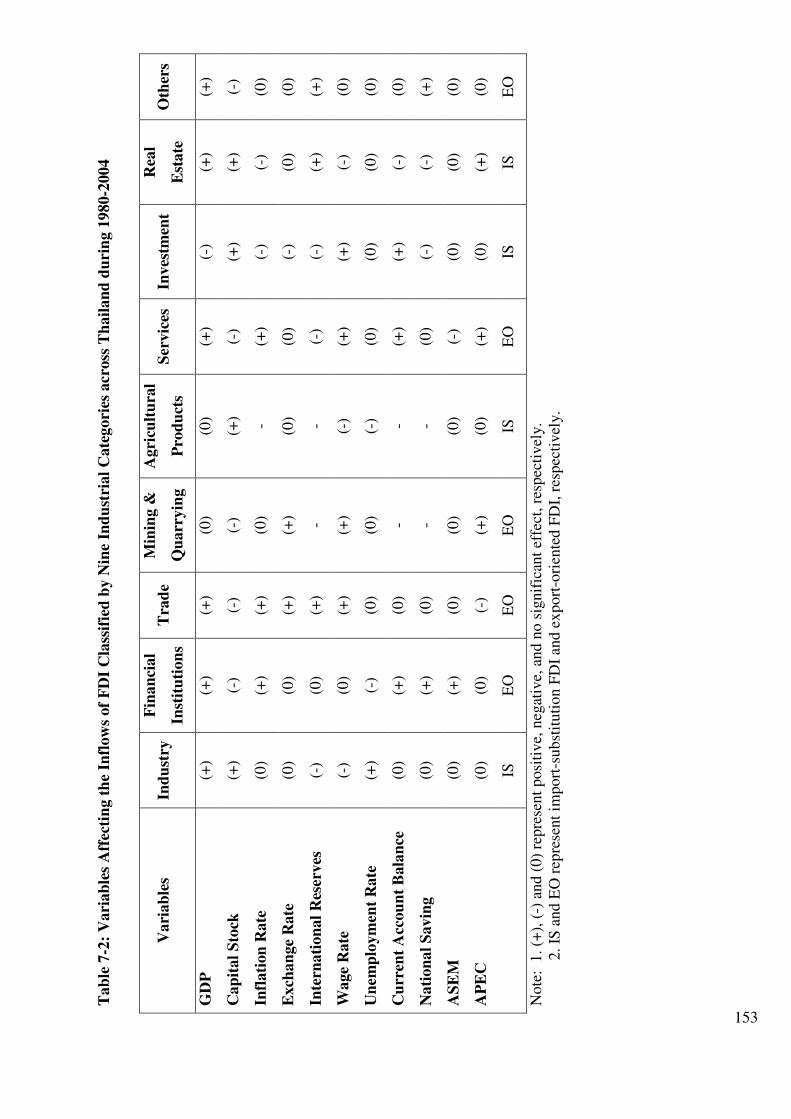
153
Tab
le 7
-2:
Vari
ab
les
Aff
ecti
ng t
he
Infl
ow
s of
FD
I C
lass
ifie
d b
y N
ine
Ind
ust
rial
Cate
gori
es a
cross
Th
ail
an
d d
uri
ng 1
980-2
004
Vari
ab
les
Ind
ust
ry
Fin
an
cial
Inst
itu
tion
s T
rad
e M
inin
g &
Qu
arr
yin
g
Agri
cult
ura
l
Pro
du
cts
Ser
vic
es
Inves
tmen
t R
eal
Est
ate
O
ther
s
GD
P
(+)
(+)
(+)
(0)
(0)
(+)
(-)
(+)
(+)
Cap
ital
Sto
ck
(+)
(-)
(-)
(-)
(+)
(-)
(+)
(+)
(-)
Infl
ati
on
Rate
(0
) (+
) (+
) (0
) -
(+)
(-)
(-)
(0)
Exch
an
ge
Rate
(0
) (0
) (+
) (+
) (0
) (0
) (-
) (0
) (0
)
Inte
rnati
on
al
Res
erves
(-
) (0
) (+
) -
- (-
) (-
) (+
) (+
)
Wage
Rate
(-
) (0
) (+
) (+
) (-
) (+
) (+
) (-
) (0
)
Un
emp
loym
ent
Rate
(+
) (-
) (0
) (0
) (-
) (0
) (0
) (0
) (0
)
Cu
rren
t A
ccou
nt
Bala
nce
(0
) (+
) (0
) -
- (+
) (+
) (-
) (0
)
Nati
on
al
Savin
g
(0)
(+)
(0)
- -
(0)
(-)
(-)
(+)
AS
EM
(0
) (+
) (0
) (0
) (0
) (-
) (0
) (0
) (0
)
AP
EC
(0
) (0
) (-
) (+
) (0
) (+
) (0
) (+
) (0
)
IS
E
O
EO
E
O
IS
EO
IS
IS
E
O
Note
: 1
. (+
), (
-) a
nd (
0)
repre
sent
posi
tive,
neg
ativ
e, a
nd n
o s
ignif
ican
t ef
fect
, re
spec
tivel
y.
2.
IS a
nd E
O r
epre
sent
import
-subst
ituti
on F
DI
and e
xport
-ori
ente
d F
DI,
res
pec
tivel
y.
154
� Wage rate has a negative impact on import-substitution FDI. A low domestic labour
wage can reduce the production costs and the prices of goods in the domestic market.
The Thai government attracts the inflows of FDI into the industry, agricultural products,
investment, and real estate categories, to increase the income for people in the country.
On the other hand, a positive impact of wage rate is found in the trade, services, and
investment categories, which recruits fewer workers than the industry and agricultural
products categories. This shows that FDI in trade, services, and investment categories
benefit workers and derive higher value-added activities or productivities from their
workers.
7.2 Policy Implications of the Study Findings
The findings of this study have important implications for policy makers in Thailand,
foreign investors and domestic investors. The findings yield some suggestions for policy
makers to enhance the attractiveness of a host country, promote and develop programmes
in order to attract more foreign investors and to sustain economic development.
With respect to regional integration and the inflows of foreign investment into Thailand,
the empirical findings can help the government to identify structural differences and how
to satisfy the needs of foreign investors. However, Thailand had faced political instability
with coups d’état, which occurred three times during the study period: 1981, 1985, 1991,
and the latest in 2006. This can be an impediment to attract more FDI. The Thai
government should make a concerted effort to reduce the political negative impact on
potential foreign investors. Governmental agencies such as BOI, BOT, the Ministry of
Commerce, and the Ministry of Industry should design and implement “friendly”
investment policies to promote both foreign and domestic industries in Thailand and to
improve the investment climate to sustain FDI and stimulate economic growth.
Thailand had enjoyed remarkable capital flows in the 1980s until the first half of the 1990s
but signs of economic instability appeared thereafter. Since the establishment of BIBF in
1993, FDI in the real estate category got into trouble in 1994 after the collapse of the FDI
financial institutions category in 1992 (see Table 2-3). At the beginning of 1996, the
Thailand economy was heading towards a crisis with speculative attacks from hedge-funds
speculators in November and again in February and May of 1997 (see Siamvalla et al.,
155
1999). The main turning point came with a significant drop in export growth rate. This
drop was due to the lack of technical, managerial, and organisational understanding in
attracting and sustaining foreign investments. In September 1996, this situation became
worse due to stagnate real estate and the external funds used to repay foreign financial
institutions. According to the empirical results, the inflows of foreign portfolio investment
depended on the health of Thai economy. The Thai government and BOT should reduce
the information and transaction costs, negotiate with investors’ governments, increase the
number of trades, and minimise the Thai Baht volatility. Stable monetary policy and
financial stability in Thailand would increase the numbers of foreign portfolio investors
into the country. The results suggest that the relative economic performances in GDP per
capita and trade of the 21 investing partners determines the levels of capital inflows into
Thailand. The booming economic activity in the economies of the investing partners
changes the flows of FDI into Thailand. Therefore, the Thai government must be prudent
and proactive in attracting more FDI into Thailand by improving investor confidence and
investment climate.
The results also show that the 1997 Asian Financial Crisis positively affected the amount
of capital inflows, but did not affect FDI. For example, portfolio investments were
positively affected by the depreciation of the Thai Baht during the financial crisis because
portfolio investors enjoyed lower transaction, information, and capital costs. Foreign
investors who engaged in exporting finished goods and components into the global market
enjoyed improved price competitiveness as a result of the depreciated Thai Baht. The
results suggest that most FDI production is export-oriented, especially in the trade
category.
In contrast, the empirical results show that an appreciation of the Thai Baht increases the
inflows of FDI into Thailand. This shows fixed investment such as machinery, installation,
raw materials, and components which are imported from overseas, is the major area of
investment for foreign direct investors. Consequently, Thailand is faced with a choice of
either strengthening or weakening against all investing partners’ currencies. Policy makers
should consider more carefully whether FDI or portfolio investment, is the more suitable to
the Thai economy at the time. However, the FDI theory suggests that FDI can reduce the
unemployment rate, transfer new and advanced technology and increase the GDP of the
country.
156
Table 7-2 shows the effects of the inflows of FDI classified by nine industrial categories
across Thailand during 1980-2004. Import-substitution is Thailand’s main strategy for
stimulating economic development, which encourages industrial growth within the country
by reducing import of goods and services. In contrast, an export-oriented strategy is an
economic policy to accelerate the industrialisation process of Thailand through exporting
to improve national income and productivity. Separating FDI strategy into two parts such
as import-substitution and export-oriented is a better way for the Thai government to
improve the production growth rate and to examine the direction of FDI in the future. The
role of FDI differs in terms of the investment strategies of the Thai government compared
to foreign investors. The global market may need a larger focus on export-oriented FDI to
design and supply products and services, whereas a domestic market focuses on import-
substitution FDI. International customers differ from domestic customers and product
design can be changed to match differences in product expectations and the income level
of customers. Specific FDI for either domestic or international customers can ensure the
highest possible returns on capital resources and profits. At the same time, it is well
understood by the Thai government that by establishing promotional privileges, it can
attract appropriate FDI to either import-substitution or export-oriented production.
There is another way to improve the attractiveness of Thailand and encourage FDI into
Thailand. Improving the investment environment and standard of services is essential to
enhance Thailand’s image. A (more) stable investment environment can be built up via
government agencies such as the Ex-Im Bank, BOI and BOT, and/or private sector
agencies such as commercial banks, transportation, and high-technological companies.
Good governance should be used to manage and supervise FDI to ensure that investments
are sustainable.
According to the empirical results, local suppliers attract more FDI. Therefore, the Thai
government should aim to increase the numbers of local suppliers and hence increase FDI.
Linkages between FDI and domestically owned firms are important to Thailand, because
the skilled, informational, behavioural, and cultural gaps between FDI and local supplier
firms are often referred to as the main impediments to any investment relationship between
the foreign investors and Thailand. FDI in the same industry category may source their
inputs differently. For example, Japanese and American investors show differences in
157
their sourcing behaviour. Thailand and Japan have a closer relationship and similar culture
compared to the US but if Thailand would like to attract American investors, the Thai
government has to assist potential local suppliers to improve their capacities to meet the
US and other investors. The Thai government should set up a national database of
potential local suppliers to match FDI with local suppliers. This is because it is difficult
for local suppliers to arrange procurement networks with foreign investors by themselves.
For example, in the 1990s, Japanese investors were particularly interested in supporting the
autoparts and electrical/electronics parts industry in Thailand. Therefore, the Department
of Industrial Promotion (DIP) in Thailand formed a master plan to support both industries
called the “Study on Industrial Sector Development – Supporting Industries in the
Kingdom of Thailand” (Lauridsen, 2004, p. 576). This plan was conducted in six parts:
policy and legislation, technology upgrading, market development, financial support,
upgrading of management, and investment promotion. As a result of this plan, most of the
Japanese investment that flowed into Thailand was concentrated in the automotive and
electrical/electronics parts industries, which enhanced the trading relationship between the
two countries. Consequently, the success of these industries attracted a large number of
foreign investments, which would have otherwise flowed into Thailand’s neighbouring
competitors. The master plan has continued to support the automotive sector in Thailand
and this has attracted US investors to establish General Motors (automotive industry) in
Thailand in 1997 because of the comprehensive automotive policy of the Thai government.
Without this policy, investors may have invested in other countries instead of Thailand.
During the Asian Financial Crisis, the government tried to integrate macroeconomic
policies and financial sector reforms without addressing the local suppliers’ problems. In
late 1998, foreign investors had increased their stakes in the financial sector, which had a
great influence on the Thai government. This led the Thai government to seek out a new
sector which could strengthen economic growth in Thailand. Therefore, local suppliers are
an important economic resource for Thailand to improve its investment climate. Prime
Minister Thaksin Shinawatra (2001-2005) argued that export-oriented production should
be supported by using local knowledge and technology to promote Thai products. In
addition, promotion of low interest loans to local suppliers through state agencies and
commercial banks was launched to support the local suppliers financially. BOI supported
Thai-owned suppliers with the promotional privileges programme that was offered to only
foreign investors. Japanese agencies such as the Japan International Cooperation Agency
158
(JICA) used their financial leverage with low interest rates to support industries in
Thailand. In addition, the World Bank also supported local suppliers with high interest
rate loans. These examples show a strong relationship between the Thai government and
external organisations which show how the Thai government helped to improve local
production to assist the economy recovery from the 1997 Asian Financial Crisis. Thus, the
supporting industries and investment (both internal and external environment) policy can
increase the investment environment in Thailand and may increase the inflows of FDI into
Thailand. In order to increase and sustain FDI in Thailand, the Thai government and its
related agencies should continue to seek local products and parts and ensure that they are
difficult to duplicate. Improvements in the support for local suppliers such as labour
training, technological assistance and marketing, should also be improved.
The quality and value of FDI needs to be improved. Concerns before, during and after the
1997 Asian Financial Crisis should be addressed. The results show that the determinants
of foreign portfolio investors depend on the health of Thai economy because changes in
Thai financial and political structure can negatively affect the inflows of portfolio
investment. At the beginning of 2006, an increased US current account deficit and the
prospect of a weakening dollar prompted funds to move into Asia including Thailand. In
December 2006, BOT announced that 30% of capital reserves would now require 30% of
foreign exchange reserves for all new foreign currency inflows into Thailand, to manage
what would otherwise be an uncontrollable amount of external funds into the country.
Every investor who wished to invest $100 would be allowed to convert only $70 into Thai
Baht to invest in the Thai market, while the remaining $30 would have to be deposited into
an interest-free account. The purpose of this directive is to tighten restrictions on local
financial institutions. Unfortunately, the BOT actions showed a lack of understanding of
investor sentiments and knowledge of how international investors form expectations and
react to various control measures. This caused a decrease of more than 100 points of the
SET index in one day. This policy not only affected the Thailand stock market but it also
weakened the Thai Baht and shook public and investor confidence. This BOT policy
showed political uncertainty. However, this did not cause all foreign investors to panic and
pull out of Thailand immediately. Since January 2007, all new FDI and portfolio
investments have been excluded from these measures. Recently, BOT has relaxed the
regulation of 30% of capital reserves by allowing FDI to deposit with financial institutions
abroad without the need to seek approval. Furthermore, the results show foreign investors
159
prefer to invest in countries with a high degree of openness, low tariff barriers and
conductive investment climate. Therefore, our findings show foreign investors have more
bargaining power, such as indirectly influencing some of the countries’ trade policy. Our
results also support the findings of Cuevas et al. (2005) that an investing country would
delay investment until the host country provides exceptional investment incentives.
Providing more generous incentives to foreign investors may be the only way to maintain
and attract FDI into Thailand.
The empirical results suggest that the inflows of FDI are driven by investing partners’
economic situations but the Thai government can take the initiative to increase the inflows
of foreign investment. Understanding the behaviour of FDI and impulsive investment in
Thailand are necessary. For example, the results show regional integration dummy
variables positively affect the FDI models. This implies foreign investors would like the
Thai government to reduce the trade and investment barriers and improve the investment
climate amongst members. Thus, investment and trade agreements, whether implemented
unilaterally or bilaterally, will enhance potential investment flows between Thailand,
investing countries and the region. In addition, in terms of investment promotion, it is
important for Thailand to establish trade agreements, such as bilateral investment treaties
(BITs) and free trade agreements (FTA), to extend linkages to other regions to increase
inflows of FDI.
To attract more capital inflows, Thailand needs to stabilise the macroeconomic
environment, facilitate financial development and steadily liberalise the financial sector
with caution. Thailand has abundant labour and resources, which are basic requirements
for FDI. Therefore, increasing the confidence of investors is the most important task for
the Thai government. In addition, trade agreements are important factors in attracting FDI
into Thailand. Export-oriented production is promoted in Thailand with product
distribution as the main objective for investors. Promoting Thailand as a first choice for
FDI includes removing trade and investment barriers to promote the free flow of goods,
services, and capital.
Economic variables such as exchange rate, GDP, capital stock, and wage rate have
significant effects on the level of FDI in our findings. As discussed in Chapter 5, Thailand
is endowed with abundant labour. The results show high wage rates deters FDI while a
160
high unemployment rate attracts FDI, especially in industrial categories such as general
industry, agricultural products, and real estate categories. This suggests that the Thai
government should make sure that labour wages remain competitive and increase training
opportunities to increase workers’ productivity to support a move from an import-
substitution to an export-oriented economy in the near future. A high inflation rate
indicates a weak currency which discourages investors. However, the results show the
inflation rate in Thailand affected export-oriented FDI such as financial institutions, trade,
and service categories. The inflation rate does not show significant results with the inflows
of import-substitution FDI. An increase in the inflation rate implies a decrease in the
purchasing power of domestic customers which redirects FDI to produce products for
overseas where the inflation rate is stable. Excessive inflation may be caused by large
government expenditure. Therefore, policy makers should consider these issues when
implementing and introducing new FDI policies.
7.3 Limitations of the Study
There are limitations in this study pertaining to the data set, the estimation techniques, and
the variables used.
� The sample size used in this study is limited to the number of investing partners on the
information provided by the BOT. Although the data set includes more than 90% of
total FDI inflows from the 21 investing partners, some investing partners such as India
and Taiwan and Thailand’s neighbours such as Laos, Vietnam, Myanmar, and
Cambodia are excluded due to a lack of available information. A comparative study
among Thailand’s neighbours, especially ASEAN members would improve the research
results.
� In addition, 16 out of 21 investing partners in this study are members of ASEM but only
nine are APEC members. This may lead to biased estimates of the impact of regional
integration on the inflows of FDI and portfolio investment.
� The models in this study do not consider political measures, human capital endowment,
government expenditures, and investment risks. This is because this study focused on
the economic relationships between Thailand and its investing partners. However, some
macroeconomic variables such as inflation rate, exchange rate, unemployment rate, and
wage rate can be influenced by government policies and political changes.
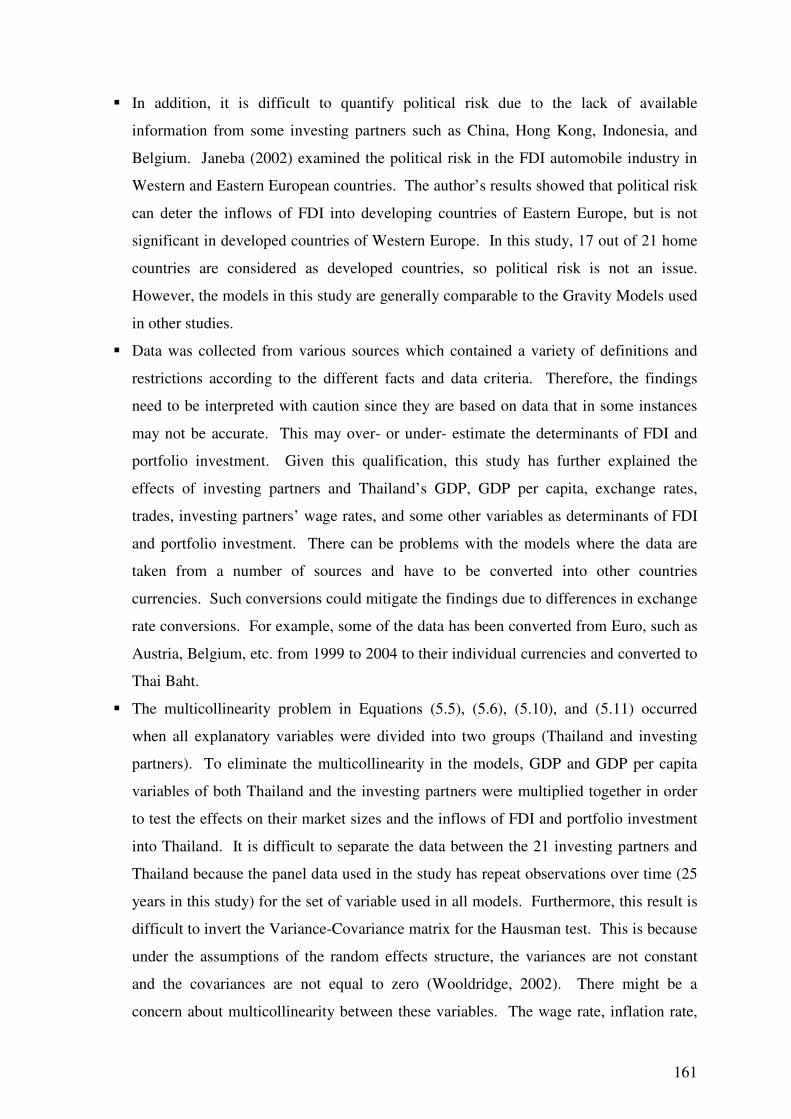
161
� In addition, it is difficult to quantify political risk due to the lack of available
information from some investing partners such as China, Hong Kong, Indonesia, and
Belgium. Janeba (2002) examined the political risk in the FDI automobile industry in
Western and Eastern European countries. The author’s results showed that political risk
can deter the inflows of FDI into developing countries of Eastern Europe, but is not
significant in developed countries of Western Europe. In this study, 17 out of 21 home
countries are considered as developed countries, so political risk is not an issue.
However, the models in this study are generally comparable to the Gravity Models used
in other studies.
� Data was collected from various sources which contained a variety of definitions and
restrictions according to the different facts and data criteria. Therefore, the findings
need to be interpreted with caution since they are based on data that in some instances
may not be accurate. This may over- or under- estimate the determinants of FDI and
portfolio investment. Given this qualification, this study has further explained the
effects of investing partners and Thailand’s GDP, GDP per capita, exchange rates,
trades, investing partners’ wage rates, and some other variables as determinants of FDI
and portfolio investment. There can be problems with the models where the data are
taken from a number of sources and have to be converted into other countries
currencies. Such conversions could mitigate the findings due to differences in exchange
rate conversions. For example, some of the data has been converted from Euro, such as
Austria, Belgium, etc. from 1999 to 2004 to their individual currencies and converted to
Thai Baht.
� The multicollinearity problem in Equations (5.5), (5.6), (5.10), and (5.11) occurred
when all explanatory variables were divided into two groups (Thailand and investing
partners). To eliminate the multicollinearity in the models, GDP and GDP per capita
variables of both Thailand and the investing partners were multiplied together in order
to test the effects on their market sizes and the inflows of FDI and portfolio investment
into Thailand. It is difficult to separate the data between the 21 investing partners and
Thailand because the panel data used in the study has repeat observations over time (25
years in this study) for the set of variable used in all models. Furthermore, this result is
difficult to invert the Variance-Covariance matrix for the Hausman test. This is because
under the assumptions of the random effects structure, the variances are not constant
and the covariances are not equal to zero (Wooldridge, 2002). There might be a
concern about multicollinearity between these variables. The wage rate, inflation rate,
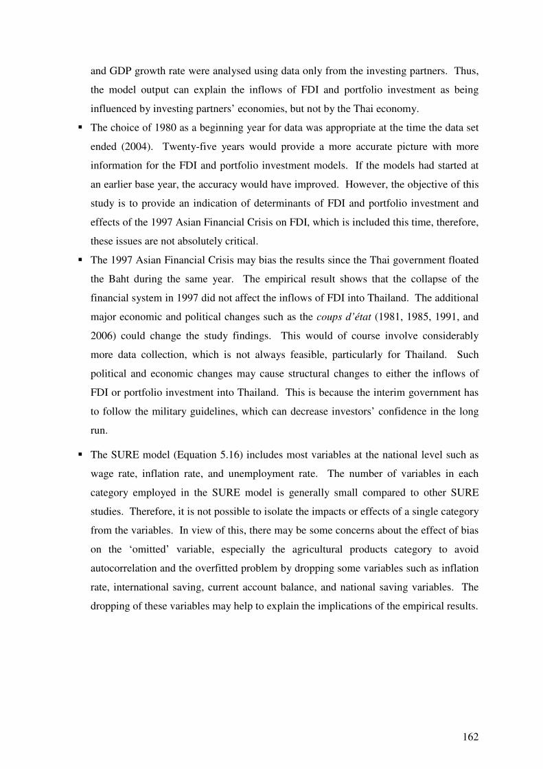
162
and GDP growth rate were analysed using data only from the investing partners. Thus,
the model output can explain the inflows of FDI and portfolio investment as being
influenced by investing partners’ economies, but not by the Thai economy.
� The choice of 1980 as a beginning year for data was appropriate at the time the data set
ended (2004). Twenty-five years would provide a more accurate picture with more
information for the FDI and portfolio investment models. If the models had started at
an earlier base year, the accuracy would have improved. However, the objective of this
study is to provide an indication of determinants of FDI and portfolio investment and
effects of the 1997 Asian Financial Crisis on FDI, which is included this time, therefore,
these issues are not absolutely critical.
� The 1997 Asian Financial Crisis may bias the results since the Thai government floated
the Baht during the same year. The empirical result shows that the collapse of the
financial system in 1997 did not affect the inflows of FDI into Thailand. The additional
major economic and political changes such as the coups d’état (1981, 1985, 1991, and
2006) could change the study findings. This would of course involve considerably
more data collection, which is not always feasible, particularly for Thailand. Such
political and economic changes may cause structural changes to either the inflows of
FDI or portfolio investment into Thailand. This is because the interim government has
to follow the military guidelines, which can decrease investors’ confidence in the long
run.
� The SURE model (Equation 5.16) includes most variables at the national level such as
wage rate, inflation rate, and unemployment rate. The number of variables in each
category employed in the SURE model is generally small compared to other SURE
studies. Therefore, it is not possible to isolate the impacts or effects of a single category
from the variables. In view of this, there may be some concerns about the effect of bias
on the ‘omitted’ variable, especially the agricultural products category to avoid
autocorrelation and the overfitted problem by dropping some variables such as inflation
rate, international saving, current account balance, and national saving variables. The
dropping of these variables may help to explain the implications of the empirical results.
163
7.4 Contribution to the Literature Review
Previous studies on FDI focus on how factors such as exchange rates, trade, and GDP
affect the firm-level decisions (see Chandprapalert, 2000; Deichman, 2004; Gao, 2005).
The aggregate-level in prior FDI studies has been ignored. In addition, there is no
empirical research that systematically compares FDI and portfolio investment and FDI
across industries at the aggregate-level. This study employs the extended Gravity Model to
determine the inflows of FDI and portfolio investment into Thailand. The extended
Gravity Model has been frequently used to examine the movement of FDI across countries
(Buch et al., 2003). However, previous Gravity Model studies have largely ignored some
of the macroeconomic factors such as inflation rate, GDP per capital, GDP growth rate,
and wage rate. This study includes macroeconomic factors such as trade, exchange rate,
national income, wage rate, regional trade and investment associations such as APEC and
ASEM, and the 1997 Asian Financial Crisis. The empirical models in this study present
more robust results in explaining the supply (from the original country) and demand (from
the recipient country) factors affecting the inflows of FDI and portfolio investment into
Thailand.
Previous researches show a positive relationship between regional trade and investment
associations and the inflows of foreign investment. However, the findings of this study
show that regional trade and investment associations have negative impacts on the inflows
of FDI and portfolio investment. This implies that the investing partners would delay their
investment until the host country (Thailand in this case) provides exceptional investment
incentives to meet their investments demand (see Biessen, 1991; Brenton et al., 1999;
Portes and Rey, 2005). The results of this study clearly explain the influence of
international asset flows. The international markets are not frictionless because countries
have different demand and supply characteristics, which heavily influence their
international transactions. This can show a different scheme of the regional associations.
Therefore, the wider range of knowledge may provide worthy guidance to the researchers
dealing with similar problems in the future.
The extended Gravity Model can be successfully implemented to determine the flows of
investment across countries. However, the results of our study show that the extended
Gravity Model does not necessarily perform better in analysing inflow FDI than portfolio
164
investment. The Breusch and Pagan test is used to test the null hypothesis of common
intercept. The results of the Hausman test in our study show that the FEM performs better
than the REM in the FDI model, but the REM is more suitable for the portfolio investment
model. This is because the REM model yields specific effects in each individual investing
partner. Consequently, the portfolio investment model reveals that time-specific are
appropriate but the FDI model is not significant to the specific time.
Finally, this study examines the inflows of FDI across industrial categories using the
SURE methodology. This is the first attempt to incorporate the regional integration such
as APEC and ASEM into the model. The results show APEC and ASEM significantly
impact the inflows of FDI across industrial categories. The inclusion of the regional
integration dummy variables provided another alternative in improving the overall fit of
the model in this study. Moreover, this suggests that other external factors can be viewed
and integrated as a measure of foreign activities. This may yield alternative explanations
of a transaction links between countries.
7.5 Suggestions for Future Study
To improve the study models and results, this section suggests some recommendations for
further studies. There are very few studies that examine FDI and portfolio investment in
Thailand using the Gravity Model. Research on FDI and portfolio investment in Thailand
has increased in recent years but many questions still remain unanswered. In this study,
the extended Gravity Model is used to determine the inflows of FDI and portfolio
investment into Thailand from 21 investing partners during 1980-2004. The following
section provides some areas that could be of interest for future study.
Empirical studies on FDI appear to focus on the developed countries (both host and home
countries). Future studies on the determinants of FDI could focus on home and host of
developing countries in different regions such as FDI flows between Thailand and the
Latin American Countries. This is to investigate the FDI trend in these two regions and to
consider the possible factors affecting the flow of FDI into these countries with similar
economic structures, such as low labour costs, same level of technology, similar natural
resources, but different culture. It may be useful for policy makers in the two regions to
develop their FDI environments to complement each other. In addition, the results may
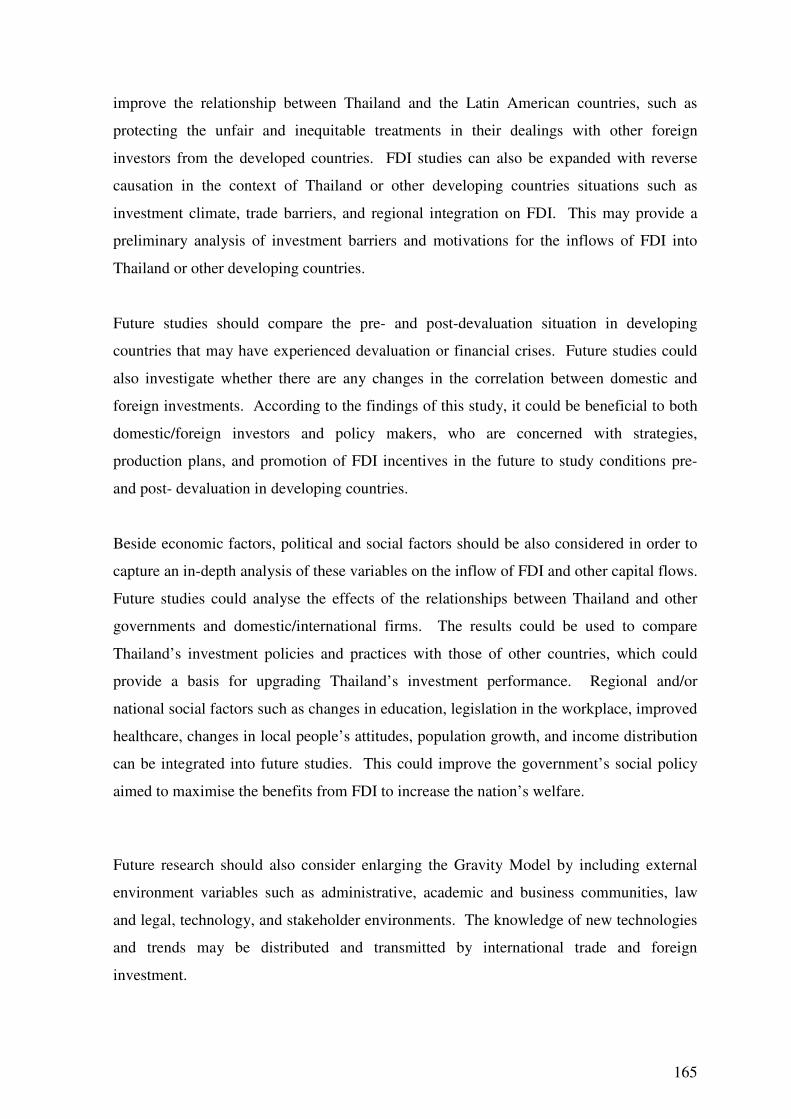
165
improve the relationship between Thailand and the Latin American countries, such as
protecting the unfair and inequitable treatments in their dealings with other foreign
investors from the developed countries. FDI studies can also be expanded with reverse
causation in the context of Thailand or other developing countries situations such as
investment climate, trade barriers, and regional integration on FDI. This may provide a
preliminary analysis of investment barriers and motivations for the inflows of FDI into
Thailand or other developing countries.
Future studies should compare the pre- and post-devaluation situation in developing
countries that may have experienced devaluation or financial crises. Future studies could
also investigate whether there are any changes in the correlation between domestic and
foreign investments. According to the findings of this study, it could be beneficial to both
domestic/foreign investors and policy makers, who are concerned with strategies,
production plans, and promotion of FDI incentives in the future to study conditions pre-
and post- devaluation in developing countries.
Beside economic factors, political and social factors should be also considered in order to
capture an in-depth analysis of these variables on the inflow of FDI and other capital flows.
Future studies could analyse the effects of the relationships between Thailand and other
governments and domestic/international firms. The results could be used to compare
Thailand’s investment policies and practices with those of other countries, which could
provide a basis for upgrading Thailand’s investment performance. Regional and/or
national social factors such as changes in education, legislation in the workplace, improved
healthcare, changes in local people’s attitudes, population growth, and income distribution
can be integrated into future studies. This could improve the government’s social policy
aimed to maximise the benefits from FDI to increase the nation’s welfare.
Future research should also consider enlarging the Gravity Model by including external
environment variables such as administrative, academic and business communities, law
and legal, technology, and stakeholder environments. The knowledge of new technologies
and trends may be distributed and transmitted by international trade and foreign
investment.
166
Apart from the two regional integration dummy variables included in this study, future
research should consider adding other economic integration regions, such as Bilateral
Investment Treaties (BITs) and Free Trade Agreement (FTA), into the models. This
includes investigating the impacts of BITs and FTA on FDI in Thailand or other host
developing countries. In addition, it would be interesting to employ other variables such as
transmission channels like freight rates, transaction fees, or restriction of monetary
transfers. This will be useful for policy purposes.
The extended Gravity Model can be used to estimate the total volume of bilateral trade
between Thailand and the 21 investing partners. Moreover, the extended Gravity Model
can be used to study Thailand’s trade and investment relationships with similar Southeast
Asian countries (Malaysia, Vietnam, Indonesia, and the Philippines) by using a specific
industry framework to develop results. A comparative study between Thailand and its
neighbours may be useful for policy makers and government agencies to develop FDI
strategies and to attract more FDI into the region. In addition, the extended Gravity Model
can be developed by using quarterly or semi-annual data and can be improved with specific
goods and services such as the wine industry and wood products. This is considered useful
for investors and policy makers in specific manufacturing sectors.
It would also be useful to examine the inflows of FDI in different kinds of industry, for
example, automotive and parts, textile, electronics and electrical products, chemical and
pharmaceutical products, and rubber products. Considering these inflows would help
domestic investors, foreign investors, and policy makers to understand the nature of the
industries better, as they would be able to measure the level of resources between each
industry. The studies of specific industries would allow policy makers to develop better
strategies to attract greater inflow of FDI into Thailand. Similar studies in other industries
would enable investors and policy makers to measure the level of resources in order to
extend product lines and increase investment.
Finally, future research should consider modelling, for example, governance of host and
home countries, capital market development, special concessions/privileges for (foreign)
investors, environmental regulations, and factors that may be significant drivers of foreign
investment. This will provide more robust policy inferences.
167
REFERENCES Adam, B., Yim-Yu, W., & Zoe, C. (2003). Traditional Medicine in China Today:
Implications for Indigenous Health Systems in a Modern World. American Journal
of Public Health, 93(7), 1082. Agarwal, S., & Ramaswami, S. (1992). Choice of Foreign Entry Mode: Impact of
Ownership, Location and Internalization Factors. Journal of International Business
Studies, 23(1), 1-27. Ahmad, Y.S, et al. (2004). “Foreign Direct Investment Versus Portfolio Investment: A
Global Games Approach”, Working Paper 05-03, University of Wisconsin- Whitewater.
Aizenman, J., & Marion, N. (2004). The Merits of Horizontal versus Vertical FDI in the
Presence of Uncertainty. Journal of International Economics, 62(1), 125. Anderson, E., & Gatignon, H. (1986). Modes of Foreign Entry: A Transaction Cost
Analysis and Propositions. Journal of International Business Studies, 17(3), 1. Anderson, J. E. (1979). A Theoretical Foundation for the Gravity Equation. The American
Economic Review, 69(1), 106. Anderson, J. E., & Wincoop, E. v. (2003). Gravity with Gravitas: A Solution to the Border
Puzzle. The American Economic Review, 93(1), 170. Annett, A. (2001). Social Fractionalization, Political Instability, and the Size of the
Government. IMF Staff Papers, 48(3/4), 561. Ansoff, H. I. (1984). Implanting Strategic Management. Englewood Cliffs, N.J.:
Prentice/Hall International. Association of Southeast Asian Nations (ASEAN). (2004). ASEAN Statistical Yearbook
2004. Backman, M., & Butler, C. (2003). Big in Asia: 25 strategies for business success.
Houndmills England; New York: Palgrave Macmillan. Bagnai, A., & Manzocchi, S. (1999). Current-Account Reversals in Developing Countries:
The Role of Fundamentals. Open Economies Review, 10(2), 143. Bajo-Rubio, O., & Sosvilla-Rivero, S. (1994). An Econometric Analysis of Foreign Direct
Investment in Spain, 1964-89. Southern Economic Journal, 61(1), 104.
Balasubramanyam, V. N., David, S., & David, G. (2002). Regional Integration Agreements and Foreign Direct Investment: Theory and Preliminary Evidence. The Manchester
School, 70(3), 460. Baltagi, B. H. (2005). Econometric Analysis of Panel Data (3rd ed.). Chichester; Hoboken,
NJ: J. Wiley & Sons.
168
Bank of Thailand. (2004). Retrieved February 19, 2005, from Web Site: http://www.bot.or.th
Bank of Thailand (2004). Quarterly Bulletin. Retrieved February 19, 2005, from http://www.bot.or.th/BOThomepage/databank/ArticlesAndPublications/ quarter_report_e.htm
Barney, J. (1991). Firm Resources and Sustained Competitive Advantage. Journal of
Management, 17(1), 99. Barney, J. (2001). Gaining and Sustaining Competitive Advantage (2nd ed.). Upper Saddle
River, NJ: Prentice Hall. Beamish, P. W. (2000). International Management: Text and Cases (4th ed.). Boston:
Irwin McGraw-Hill. Becker, G. S. (1976). The Economic Approach to Human Behavior. Chicago: University of
Chicago Press. Bergstrand, J. H. (1985). The Gravity Equation in International Trade: Some
Microeconomic Foundations and Empirical Evidence. The Review of Economics
and Statistics, 67(3), 474. Bergstrand, J. H. (1989). The Generalized Gravity Equation, Monopolistic Competition,
and the Factor-Proportions Theory in International Trade. The Review of
Economics and Statistics, 71(1), 143. Bettis, R. A. (1981). Performance Differences in Related and Unrelated Diversified Firms.
Strategic Management Journal (pre-1986), 2(4), 379. Bevan, A. A., & Estrin, S. (2004). The Determinants of Foreign Direct Investment into
European Transition Economies. Journal of Comparative Economics, 32(4), 775. Biessen, G. (1991). Is the Impact of Central Planning on the Level of Foreign Trade Really
Negative? Journal of Comparative Economics, 15(1), 22. Binh, N. N., & Haughton, J. (2002). Trade Liberalization and Foreign Direct Investment in
Vietnam. ASEAN Economic Bulletin, 19(3), 302. Blomström, M. & Kokko, A. (1997). “How Foreign Investment Affects Host Countries”,
Policy Research Working Paper, International Economic Department, The World Bank.
Blonigen, B. A. (1997). Firm-Specific Assets and the Link between Exchange Rates and
Foreign Direct Investment. The American Economic Review, 87(3), 447. Boddewyn, J. J. (1988). Political Aspects of MNE Theory. Journal of International
Business Studies, 19(3), 341.
169
BOI. (2005). Foreign Investment. Retrieve February 20, 2005, from http://www.boi.go.th/english/about/statistics_investment.asp
BOT (2004). Quarterly Bulletin. Retrieved February 19, 2005, from
http://www.bot.or.th/BOThomepage/databank/ArticlesAndPublications/ quarter_report_e.htm
BOT: Bank of Thailand (2005). http://www.bot.or.th/bothomepage/databank/EconData/
EconFinance/Download/Tab89.xls Bougheas, S., Demetriades, P. O., & Morgenroth, E. L. W. (1999). Infrastructure,
Transport Costs and Trade. Journal of International Economics, 47(1), 169-189. Bowman, C., & Asch, D. C. (1987). Strategic Management. Basingstoke: Macmillan. Brenton, P., Mauro, F. D., & Lucke, M. (1999). Economic integration and FDI: An
Empirical Analysis of Foreign Investment in the EU and in Central and Eastern Europe. Empirica, 26(2), 95.
Brewer, T. L. (1993). Government Policies, Market Imperfections, and Foreign Direct
Investment. Journal of International Business Studies, 24(1), 101. Brimble, P., & Sibunruang, A. (2002, 16-17 August). Foreign Direct Investment:
Performance and Attraction; The Case of Thailand. Paper presented at the Workshop on Foreign Direct Investment: Opportunities and Challenges for Cambodia, Laos and Vietnam, Hanoi, Vietnam.
Brooks, D. H., Fan, E. X., & Sumulong, L. R. (2003). Foreign Direct Investment in
Developing Asia: Trends, Effects, and Likely issues for the Forthcoming WTO
Negotiations: Asian Development Bank. Brown, R., & Gutterman, A. S. (2003). A Short Course in International Business Plans :
Charting a Strategy for Success in Global Commerce. Novato, Calif: World Trade Press.
Buch, C. M., Kokta, R. M., & Piazolo, D. (2003). Foreign Direct Investment in Europe: Is
There Redirection from the South to the East? Journal of Comparative Economics,
31(1), 94. Buckley, P. J., & Casson, M. (1981). The Optimal Timing of a Foreign Direct Investment.
The Economic Journal, 91(361), 75. Buckley, P. J., Clegg, J., Forsans, N., & Reilly, K. T. (2003). Evolution of FDI in the
United States in the Context of Trade Liberalization and Regionalization. Journal
of Business Research, 56(10), 853. Caldeira, M. M., & Ward, J. M. (2003). Using Resource-Based Theory to Interpret the
Successful Adoption and Use of Information Systems and Technology in Manufacturing Small and Medium-Sized Enterprises. European Journal of
Information Systems, 12(2), 127.
170
Calvet, A. L. (1981). A Synthesis of Foreign Direct Investment Theories and Theories of the Multinational Firm. Journal of International Business Studies, 12(1), 43.
Carson, C. S. (2003). Foreign Direct Investment Trends and Statistics: International
Monetary Fund. Carstensen, K., & Toubal, F. (2004). Foreign Direct Investment in Central and Eastern
European Countries: A Dynamic Panel Analysis. Journal of Comparative
Economics, 32(1), 3. Casson, M. (1982). The Theory of Foreign Direct Investment. In Buckley, P. J. (Ed).
International Investment. Brookfield, USA: Elgar. Castells, M. (2000). The Rise of the Network Society (2nd ed.). Oxford, UK ; Malden, MA: Blackwell Publishers. Certo, S. C., & Peter, J. P. (1991). Strategic Management: Concepts and Applications
(2nd ed.). New York: McGraw-Hill. Chadee, D. D., & Schlichting, D. A. (1997). Foreign Direct Investment in the Asia-Pacific
Region: Overview of Recent Trends and Patterns. Asia Pacific Journal of
Marketing and Logistics, 9(3), 3. Chandler, A. D. (1977). The Visible Hand: the Managerial Revolution in American
Business. Cambridge, Mass.: Belknap Press. Chandprapalert, A. (2000). The Determinants of U.S. Direct Investment in Thailand:
A Survey on Managerial Perspectives. Multinational Business Review, 8(2), 82. Chang, W. & Alexandra, S. (2001). On the Real Effects of Net Capital Inflows: The
Experiences of Developing Countries. A Thesis Submitted in Partial Fulfilment of the Requirements for the Degree of Doctor of Philosophy at University of California, Los Angeles. Unpublished Thesis Ph D -- University of California 2001.
Chatterjee, S., & Wernerfelt, B. (1991). The Link between Resources and Type of
Diversification: Theory and Evidence. Strategic Management Journal, 12(1), 33. Chen, C.-J., & Chang, L.-S. (2004). Dynamics of Business Network Embeddedness.
Journal of American Academy of Business, Cambridge, 5(1/2), 237. Chen, T.-J., Chen, H., & Ku, Y.-H. (2004). Foreign Direct Investment and Local Linkages.
Journal of International Business Studies, 35(4), 320. Chen, H., & Chen, T.-J. (1998). Network Linkages and Location Choice in Foreign Direct
Investment. Journal of International Business Studies, 29(3), 445. Chen, T.-J., & Ku, Y.-H. (2002). Creating Competitive Advantages out of Market
Imperfections: Taiwanese Firms in China. Asian Business & Management, 1(1), 79.
171
Cheng, L. K., & Kwan, Y. K. (2000). What are the Determinants of the Location of Foreign Direct Investment? The Chinese Experience. Journal of International
Economics, 51(2), 379. Closs, D. J., & Thompson, C. K. (1992). Logistics Physical Resource Management.
Journal of Business Logistics, 13(2), 269. Cooley, P. L. (1994). Business Financial Management (3rd ed.). Fort Worth: Dryden
Press. Cortes Rodriguez, M. V. (2002). Trade between New Zealand and Latin American
Countries: a Modified Gravity Model. A Thesis Submitted in Partial Fulfilment of the Requirements for the Degree of Doctor of Philosophy (Economics) at Lincoln University. Unpublished Thesis Ph D -- Lincoln University 2002.
Courchene, T. J., & Harris, R. G. (2000). North American Monetary Union: Analytical
Principles and Operational Guidelines. North American Journal of Economics and
Finance, 11(1), 3. Cuevas, A., Messmacher, M., & Werner, A. (2005). Foreign Direct Investment in Mexico
since the Approval of NAFTA. The World Bank Economic Review, 19(3), 473. Dascal, D., Mattas, K., & Tzouvelekas, V. (2002). An Analysis of EU Wine Trade: a
Gravity Model Approach.(European Union) (Statistical Data Included). (European
Union)(Statistical Data Included), 8(2), 135(113). Davidow, W. H. (1986). Marketing High Technology: an Insider's View. New York: Free
Press. Deardorff, A.V. (1995). “Determinants of Bilateral Trade: Does Gravity Work in a
Neoclassical World?”, Working Papers Series, National Bureau of Economic Research. DeBresson, C., & Amesse, F. (1991). Networks of Innovators: A Review and Introduction
to the Issue. Research Policy, 20(5), 363-379. Deichmann, J. I. (2004). Origins of Foreign Direct Investment in Poland, 1989-2001. The
Journal of Business and Economic Studies, 10(1), 12. Diao, X., Rattso, J., & Stokke, H. E. (2005). International spillovers, productivity growth
and openness in Thailand: an intertemporal general equilibrium analysis. Journal of
Development Economics, 76(2), 429-450. Dunning, J.H. (1976). Trade, Location of Economic Activity and the MNE: A Search for
an Eclectic Approach. In B. Ohlin et al (Eds.). The International Allocation of
Economic Activity: Proceedings of a Nobel Symposium held at Stockholm, Stockholm, 8-11 June 1976. London: Macmillan Press.
Dunning, J. H. (1980). Toward an Eclectic Theory of International Production: Some
Empirical Tests. Journal of International Business Studies, 11(1), 9.
172
Dunning, J. H. (1988). Explaining International Production. London ; Boston: Unwin Hyman.
Dunning, J. H. (1998). Location and the Multinational Enterprise: A Neglected Factor?
Journal of International Business Studies, 29(1), 45. Dunning, J. H., & Gray, H. P. (2003). Extending the Eclectic Paradigm in International
Business: Essays in Honor of John Dunning. Cheltenham, UK ; Northampton, MA: Edward Elgar.
Dunning, J. H., Kim, Z. K., & Lee, C. (2007). Restructuring the regional distribution of
FDI: The case of Japanese and US FDI. Japan and the World Economy, 19(1),
26-47. Ebers, M., & Jarillo, J. C. (1998). The Construction, Forms, and Consequences of Industry
Networks. International Studies of Management & Organization, 27(4), 3. Eden, L., & Lenway, S. (2001). Introduction to the Symposium Multinationals: The Janus
Face of Globalization. Journal of International Business Studies, 32(3), 383. Egger, P., & Pfaffermayr, M. (2004a). Distance, Trade and FDI: A Hausman-Taylor SUR
Approach. Journal of Applied Econometrics, 19(2), 227-246. Egger, P., & Pfaffermayr, M. (2004b). The Impact of Bilateral Investment Treaties on
Foreign Direct Investment. Journal of Comparative Economics, 32(4), 788-804. Eicher, T., & Kang, J. W. (2005). Trade, Foreign Direct Investment or Acquisition:
Optimal Entry Modes for Multinationals. Journal of Development Economics,
77(1), 207. Elek, A. (1992). Trade Policy Options for the Asia-Pacific Region in the 1990's: The
Potential of Open Regionalism. The American Economic Review, 82(2), 74. Elmawazini, K., Saadi, S., & Ngouhouo, I. (2005). Does FDI Imply Productivity Growth
for the Host Economy? Journal of American Academy of Business, Cambridge,
6(2), 85. Erlander, S. (1980). Optimal Spatial Interaction and the Gravity Model. Berlin ; New
York: Springer-Verlag. Europa Publications Limited. (2004). The Europa World Year Book (Vol. 1-2 ed. 2004).
London, England: Europa Publications Limited Evenett, S. J., & Keller, W. (2002). On Theories Explaining the Success of the Gravity
Equation. The Journal of Political Economy, 110(2), 281. Froot, K. A., & Stein, J. C. (1991). Exchange Rates and Foreign Direct Investment: An
Imperfect Capital Markets Approach. The Quarterly Journal of Economics, 106(4), 1191.
173
Galan, J. I., & Gonzalez-Benito, J. (2001). Determinant Factors of Foreign Direct Investment: Some Empirical Evidence. European Business Review, 13(5), 269.
Gao, T. (2005). Foreign Direct Investment and Growth under Economic Integration.
Journal of International Economics, 67(1), 157. Garson, J.-P. (1998). North America: Migration and economic integration. Organisation
for Economic Cooperation and Development. The OECD Observer (214), 18. Girma, S. (2002). The Process of European Integration and the Determinants of Entry by
Non-EU Multinationals in UK Manufacturing. The Manchester School, 70(3), 315. Girod, S. J. G., & Rugman, A. M. (2005). Regional Business Networks and the
Multinational Retail Sector. Long Range Planning, 38(4), 335. Gopinath, M., & Echeverria, R. (2004). Does Economic Development Impact the Foreign
Direct Investment-Trade Relationship? A Gravity-Model Approach. American
Journal of Agricultural Economics, 86(3), 782. Gowa, J., & Mansfield, E. D. (2004). Alliances, Imperfect Markets, and Major-Power
Trade. International Organization, 58(4), 775. Grant, R. M. (1991). The Resource-Based Theory of Competitive Advantage: Implications
for Strategy Formulation. California Management Review, 33(3), 114. Greene, W. H. (2003). Econometric Analysis (5th ed.). Upper Saddle River, N.J.: Prentice
Hall. Grindley, P. C., & Teece, D. J. (1997). Managing Intellectual Capital: Licensing and
Cross-Licensing in Semiconductors and Electronics. California Management
Review, 39(2), 8. Grosse, R., & Trevino, L. J. (1996). Foreign Direct Investment in the United States: An
Analysis by Country of Origin. Journal of International Business Studies, 27(1), 139.
Guerin, S. S. (2006). The Role of Geography in Financial and Economic Integration: A
Comparative Analysis of Foreign Direct Investment, Trade and Portfolio Investment Flows. The World Economy, 29(2), 189.
Gulati, R. (1999). Network Location and Learning: The Influence of Network Resources
and Firm Capabilities on Alliance Formation. Strategic Management Journal,
20(5), 397. Gulati, R., Nohria, N., & Zaheer, A. (2000). Strategic Networks. Strategic Management
Journal, 21(3), 203. Haddad, M., & Harrison, A. (1993). Are There Positive Spillovers from Direct Foreign
Investment? Evidence from Panel Data for Morocco. Journal of Development
Economics, 42(1), 51.
174
Hakansson, H. & Johanson, J. (1993). The Network as a Governance Structure: Inter- Firm Cooperation beyond Markets and Hierarchies. In Grabher G. (Ed) The
Embedded Firm: On the Socioeconomics of Industrial Networks. London: Routledge.
Hall, R. (1992). The Strategic Analysis of Intangible Resources. Strategic Management
Journal, 13(2), 135. Hartman, D. G. (1984). Tax Policy and Foreign Direct Investment in the United States.
National Tax Journal, 37(4), 475. Harvey, D. F., & Bowin, R. B. (1996). Human resource Management: an Experiential
Approach. Upper Saddle River, N.J.: Prentice Hall. Head, C. K., Ries, J. C., & Swenson, D. L. (1999). Attracting Foreign Manufacturing:
Investment Promotion and Agglomeration. Regional Science and Urban
Economics, 29(2), 197. Helpman, E. (1984). A Simple Theory of International Trade with Multinational
Corporations. The Journal of Political Economy, 92(3), 451. Helpman, E. (1987). Imperfect Competition and International Trade: Opening Remarks.
European Economic Review, 31(1,2), 77. Hill, C., Hwang, P. and Kim, W.C. (1990). An Eclectic Theory of the Choice of
International Entry Mode. Strategic Management Journal, 11, 117-128. Hill, C. W. L., & Jones, G. R. (1992). Strategic Management Theory: an Integrated
Approach (2nd ed.). Boston: Houghton Mifflin. Hymer, S. (1972). The Internationalization of Capital. Journal of Economic Issues
(pre-1986), 6(1), 91. Hongskul, V. (2000). Impact of Foreign Direct Investment on Thailand's Trade and
Domestic Private Investment. A Thesis Presented in Partial Fulfilment of the Requirements for the Degree of Master in Applied and International Economics at Massey University, Palmerston North, New Zealand. Unpublished Thesis Ph D – Massey University 2000.
How far is it. Retrieved February 15, 2005, from http://indo.com/distance/ Hubert, F., & Pain, N. (2002). Fiscal Incentives, European Integration and the Location of
Foreign Direct Investment. The Manchester School, 70(3), 336. Idris, F., Abdullah, M., Idris, M. A., & Hussain, N. (2003). Integrating Resource-Based
View and Stakeholder Theory in Developing the Malaysian Excellence Model: A Conceptual Framework. Singapore Management Review, 25(2), 91.
IMF. (1993). Balance of Payments Manual. Washington: International Monetary Fund.
175
International Monetary Fund (2003). Foreign Direct Investment Trends and Statistics.
Washington, D.C.: International Monetary Fund. International Monetary Fund (2004). International Financial Statistics Yearbook (English
ed. August 2004). Washington, D.C.: International Monetary Fund. Isard, P. (1977). How Far can We Push the "Law of One Price"? The American Economic
Review, 67(5), 942. Ismail, R., & Yussof, I. (2003). Labour Market Competitiveness and Foreign Direct
Investment: The Case of Malaysia, Thailand and the Philippines. Papers in
Regional Science, 82(3), 389. Itaki, M. (1991). A Critical Assessment of the Eclectic Theory of the Multinational
Enterprise. Journal of International Business Studies, 22(3), 445. Janeba, E. (2002). Attracting FDI in a politically risky world. International Economic
Review, 43(4), 1127. Jansen, W. J. (2003). What do Capital Inflows Do? Dissecting the Transmission
Mechanism for Thailand, 1980-1996. Journal of Macroeconomics, 25(4), 457-480. Jansen, W. J., & Stokman, A. C. J. (2004). Foreign Direct Investment and International
Business Cycle Comovement (Working Paper No. 401). Frankfurt, Germany: European Central Bank.
Jarillo, J. C. (1988). On Strategic Networks. Strategic Management Journal (1986-1998),
9(1), 31. Jiang, Z. (2003). Determinants of public listing of Chinese enterprises: Influences of
regional factors. A Thesis Submitted in Partial Fulfilment of the Requirements for the Degree of Doctor of Philosophy at Stanford University, the United States. Unpublished Thesis Ph D – Stanford University 2003.
Julian, C. C. (2001). Japanese Foreign Direct Investment in Thailand. The Mid - Atlantic
Journal of Business, 37(1), 7. Kang, M. (2003). United States Wood Products and Regional Trade: A Gravity Model
Approach. A Thesis Submitted in Partial Fulfilment of the Requirements for the Degree of Doctor of Philosophy at Auburn University, Alabama. Unpublished Thesis Ph D – Auburn University 2003.
Karami, A., Analoui, F., & Cusworth, J. (2004). Strategic Human Resource Management
and Resource-based Approach: The Evidence from the British Manufacturing Industry. Management Research News, 27(6), 50.
176
Kim, Z. (2000). The Comparison of Geographic and Industrial Patterns of Japanese and
United States Foreign Direct Investment (FDI) from the 1970s to the 1990s:
Toward Convergence? A Thesis Submitted in Partial Fulfilment of the Requirements for the Degree of Doctor of Philosophy at Rutgers The State University of New Jersey- Newark. Unpublished Thesis Ph.D. -- Rutgers The State University of New Jersey- Newark (2000).
Kohpaiboon, A. (2003). Foreign Trade Regimes and the FDI-Growth Nexus: A Case Study
of Thailand. The Journal of Development Studies, 40(2), 55. Kontoghiorghes, E. J. (2000). Parallel Strategies for Solving SURE Models with Variance
Inequalities and Positivity of Correlations Constraints. Computational Economics,
15(1-2), 89. Krugman, P. R. (1991). Geography and Trade. Cambridge, Mass.: MIT Press. Krugman, P. R. (1995). Development, Geography, and Economic Theory. Cambridge,
Mass.: MIT Press. Kumar, N. (2003). Investment on the WTO Agenda: A developing Countries Perspective
and the Way Forward for the Cancun Ministerial Conference. Paper presented at the Cancun Ministerial Conference, WTO, Cancun, Mexico.
Kumar, A., & Zajc, K. (2003). Foreign Direct Investment and Changing Trade Patterns:
The Case of Slovenia. Economic and Business Review for Central and South -
Eastern Europe, 5(3), 201. Leamer, E. E. (1993). Factor-Supply Differences as a Source of Comparative Advantage.
The American Economic Review, 83(2), 436. Limao, N., & Venables, A. J. (2001). Infrastructure, Geographical Disadvantage, Transport
Costs, and Trade. The World Bank Economic Review, 15(3), 451. Lindelöf, P., & Löfsten, H. (2004). Proximity as a Resource Base for Competitive
Advantage: University-Industry Links for Technology Transfer. Journal of
Technology Transfer, 29(3-4), 311. Loungani, P., & Razin, A. (2001). How Beneficial Is Foreign Direct. Finance &
Development (June, 2001), 6-9. Lauridsen, L. S. (2004). Foreign Direct Investment, Linkage Formation and Supplier
Development in Thailand during the 1990s: The Role of State Governance. The European Journal of Development Research, 16(3), 561.
Mallampally, P., & Sauvant, K. P. (1999). Foreign Direct Investment in Developing
Countries. Finance & Development, 36(1), 34-37. Mark, N. C., Ogaki, M., & Sul, D. (2005). Dynamic Seemingly Unrelated Cointegrating
Regressions. The Review of Economic Studies, 72(252), 797.
177
Markusen, J. R., & Maskus, K. E. (2002). Discrimination among alternative theories of the multinational enterprise. Review of International Economics, 10(4), 694.
Marr, B., Schiuma, G., & Neely, A. (2004). The Dynamics of Value Creation: Mapping
Your Intellectual Performance Drivers. Journal of Intellectual Capital, 5(2), 312. Martinez-Zarzoso, I. (2003). Gravity Model: An Application to Trade between Regional
Blocs. Atlantic Economic Journal, 31(2), 174. Martínez-Zarzoso, I., & Nowak-Lehmann D, F. (2004). Economic and Geographical
Distance: Explaining MERCOSUR Sectoral Exports to the EU. Open Economies
Review, 15(3), 291. McCallum, J. (1995). National Borders Matter: Canada-U.S. Regional Trade Patterns.
The American Economic Review, 85(3), 615. McGoldrick, J. A., Stewart, J., & Watson, S. (2002). Understanding Human Resource
Development a Research-Based Approach. London: Routledge. Mills, J., Platts, K., & Bourne, M. (2003). Applying Resource-Based Theory: Methods,
Outcomes and Utility for Managers. International Journal of Operations &
Production Management, 23(2), 148. Milner, C., Reed, G., & Talerngsri, P. (2004). Foreign Direct Investment and Vertical
Integration of Production by Japanese Multinationals in Thailand. Journal of
Comparative Economics, 32(4), 805. Mirza, H., & Giroud, A. (2004). Regional Integration and Benefits from Foreign Direct
Investment in ASEAN Economies: The Case of Viet Nam. Asian Development
Review, 21(1), 66. Mueller, T. (2001). Analyzing Modes of Foreign Entry: Greenfield Investment Versus
Acquisition. University of Munich: Mimeo. Nakamura, S. & Oyama, T. (1998). “The Determinants of Foreign Direct Investment from
Japan and the United States to East Asian Countries, and the Linkage between FDI and Trade”. Working Paper 98-11, Research and Statistics Department, The Bank of Japan.
NESDB. (2004). Retrieved March 27, 2005, from http://www.nesdb.go.th NESDB. (2005). Retrieved May 15, 2005, from http://www.nesdb.go.th Newell, S., & Swan, J. (2000). Trust and Inter-Organizational Networking. Human
Relations, 53(10), 1287. Newland, O. (2004). The Day the Bubble Bursts. Auckland, N.Z.: Empower Leaders Pub. Noorbakhsh, F., & Paloni, A. (2001). Human Capital and FDI Inflows to Developing
Countries: New empirical evidence. World Development, 29(9), 1593.
178
Pain, N., & Lansbury, M. (1997). Regional Economic Integration and Foreign Direct Investment: The Case of German Investment in Europe. National Institute
Economic Review (160), 87. Pak, Y. S., & Park, Y.-R. (2005). Characteristics of Japanese FDI in the East and the West:
Understanding the Strategic Motives of Japanese Investment. Journal of World
Business, 40(3), 254. Pedroni, P. (1999). Critical Values for Cointegration Tests in Heterogeneous Panels with
Multiple Regressors. Oxford Bulletin of Economics and Statistics, 61(s1), 653-670. Pelletiere, D., & Reinert, K. A. (2004). Used Automobile Protection and Trade: Gravity
and Ordered Probit Analysis. Empirical Economics, 29(4), 737. Penrose, E. T. (1959). The Theory of the Growth of the Firm. Oxford: B. Blackwell. Perlmutter, H. V. (1969). Some Management Problems in Spaceship Earth: The Megafirm
and the Global Industrial Estate. Academy of Management Journal (pre-1986), 12, 59.
Perron, P. (1989). The Great Cash, the Oil Price Shock, and the Unit Root Hypothesis.
Econometrica (1986-1998), 57(6), 1361. Porras, S. T., Clegg, S., & Crawford, J. (2004). Trust as Networking Knowledge:
Precedents from Australia. Asia Pacific Journal of Management, 21(3), 345. Portes, R., & Rey, H. (2005). The Determinants of Cross-Border Equity Flows. Journal of
International Economics, 65(2), 269. Ragazzi, G. (1973). “Theories of the Determinants of Direct Foreign Investment”,
IMF Staff papers, 20(2), 471. Ratnayake, R., & Townsend, B. (1999). The Geographical Pattern of New Zealand's
International Trade: An Application of the Gravity Model. New Zealand Economic
Papers, 33(2), 27-38. Ray, P. K., Ida, M., Suh, C.-S., & Rhaman, S.-U. (2004). Dynamic Capabilities of
Japanese and Korean Enterprises and the 'Flying Geese' of International Competitiveness. Asia Pacific Business Review, 10(3,4), 463.
Razin, A. (2002). FDI flows: a critical look. (Research Summaries). NBER
Reporter, p.16(3). Retrieved April 19, 2008, from General OneFile via Gale: http://find.galegroup.com/itx/start.do?prodId=ITOF
Reis, A. B. (2001). On the Welfare Effects of Foreign Investment. Journal of International
Economics, 54(2), 411. Roberto, B. (2004). Acquisition Versus Greenfield Investment: the Location of Foreign
Manufacturers in Italy. Regional Science and Urban Economics, 34(1), 3.
179
Roos, J. (1998). Exploring the Concept of Intellectual Capital (IC). Long Range Planning,
31(1), 150. Rose, A. K. (2000). One Money, One Market: The Effect of Common Currencies on
Trade. Economic Policy (30), 7. Rose, A. K., & Spiegel, M. M. (2004). A Gravity Model of Sovereign Lending: Trade,
Default, and Credit. IMF Staff Papers, 51, 50. Rosenberg, M. T. (2004). Gravity Model: Predict The Movement of People and Ideas
Between Two Places. Retrieved February 20, 2005, from Web Site: http://geography.about.com/library/weekly/aa031601a.htm?iam=dpile_1&terms =gravity
Rubesch, E., & Banomyong, R. (2005). Selecting Suppliers in the Automotive Industry: Comparing International Logistics Costs. Asia Pacific Journal of Marketing and
Logistics, 17(1), 61. Rugman, A. M. (1980). A New Theory of the Multinational Enterprise:
Internationalization Versus Internalization. Columbia Journal of World Business,
15(1), 23. Rugman, A. M. (1982). New Theories of the Multinational Enterprise. London:
Croom Helm.
Rugman, A. M. (1986). New Theories of the Multinational Enterprise: An Assessment of Internalization Theory. Bulletin of Economic Research, 38(2), 101.
Rugman, A. M. (1988). The Firm-Specific Advantages of Canadian Multinationals.
International Studies of Management & Organization, 18(1), 67. Sachs, J. D., Warner, A., Aslund, A., & Fischer, S. (1995). Economic Reform and the
Process of Global Integration; Comments. Brookings Papers on Economic Activity
(1), 1. Sally, R. (2007). Thai Trade Policy: From Non-discriminatory Liberalisation to FTAs. The
World Economy, 30(10), 1594. Sanna-Randaccio, F. (2002). The Impact of Foreign Direct Investment on Home and Host
Countries with Endogenous R&D. Review of International Economics, 10(2), 278. Sapir, A. (1997). “Domino Effects in Western European Trade, 1960-92”, Discussion
Papers, Centre of Economic Policy Research, Australian National University. Schroeder, R. G., Bates, K. A., & Junttila, M. A. (2002). A Resource-Based View of
Manufacturing Strategy and the Relationship to Manufacturing Performance. Strategic Management Journal, 23(2), 105.
180
Seo, J. S., & Suh, C.-S. (2006). An Analysis of Home Country Trade Effects of Outward Foreign Direct Investment: The Korean Experience with ASEAN, 1987-2002. ASEAN Economic Bulletin, 23(2), 160.
Shapiro, A. C. (2003). Multinational Financial Management. MA, USA: John
Wiley&Sons. Siamwalla, A., Vajragupta, Y., & Vichyanond, P. (1999). “Foreign Capital Flows to
Thailand: Determinants and Impact”. Thailand Development Research Institute, Bangkok.
Simmons, R. P. (2003). An Empirical Study of the Impact of Corporate Taxation on the
Global Allocation of Foreign Direct Investment: a Broad Tax Attractiveness Index Approach. Journal of International Accounting Auditing & Taxation, 12(2), 105.
Stock, J. H., & Watson, M. W. (2003). Introduction to Econometrics. Boston, MA:
Addison Wesley. Stone, S. F., & Jeon, B. N. (1999). Gravity-Model Specification for Foreign Direct
Investment: A Case of the Asia-Pacific Economies. The Journal of Business and
Economic Studies, 5(1), 33. Summary, R. M. (1989). A Political-Economic Model of U.S. Bilateral Trade. The Review
of Economics and Statistics, 71(1), 179. Sussangkarn, C. (1999). Economic Crisis and Recovery in Thailand: The Role of the IMF.
Thailand Development Research Institute (TDRI), Bangkok. Tangkitvanich, S, et al. (2004). Thailand. In Brooks, A. H. and Hill, H. (Eds.) Managing
FDI in a Globalizing Economy. New York: Palgrave Macmillan. Tahir, R., & Larimo, J. (2005). Understanding the Strategic Motivations of Finnish
Manufacturing FDIs in Emerging Asian Economies. Asian Business &
Management, 4(3), 293. TDRI: Thailand Development Research Institute. (2003). TDRI Quarterly Review.
Bangkok.
Teece, D. J. (1981). The Multinational Enterprise: Market Failure and Market Power Considerations. Sloan Management Review (pre-1986), 22(3), 3.
Thomsen, S. (1999). “Southeast Asia: The Role of Foreign Direct Investment Policies in
Development”, Working Papers on International Investment, OECD. Tiwari, P., Syamwil, I. B., & Doi, M. (2003). Spatial Pattern of Japanese Manufacturing
Industry in Four ASEAN Countries. Papers in Regional Science, 82(3), 403. Tuan, C., & Ng, L. F.-Y. (2004). FDI and Industrial Restructuring in Post-WTO Greater
PRD: Implications on Regional Growth in China. The World Economy, 27(10), 1609.
181
UN (1998). Trends and Determinants. World Investment Report. UNCTAD. (2004, June 15). Investment Instruments: Bilateral Investment Treaties.
Retrieved May 5, 2005, from http://www.unctadxi.org/templates/ DocSearch.aspx?id=779
UNCTAD (2004). Prospects for FDI Flows, Transnational Corporation Strategies and
Promotion Policies: 2004-2007. Retrieved April 22, 2005, from http://www. unctad.org/en/docs/tdxibpd5_en.pdf
UNCTAD. (2004). World Investment Report 2004. Message posted to www.unctad.org/fdistatistics
UNCTAD. (2005). World Investment Report 2005. Message posted to
www.unctad.org/fdistatistics Ussahawanitchakit, W. (2002). Resource-Based Determinants of Export Performance
Effects of ISO 9000 Certification. A Thesis Submitted in Partial Fulfilment of the Requirements for the Degree of Doctor of Philosophy at Washington State University, Washington. Unpublished Thesis Ph D – Washington State University 2002.
Velde, D. W. t., & Morrissey, O. (2002). Foreign Direct Investment: Who Gains? ODI
Briefing Paper, 1-4. Vernon, R. (1966) International Investment and International Trade in the Product Cycle.
Quarterly Journal of Economics, 80(May), 190. Vernon, R. (2001). Big Business and National Governments: Reshaping the Compact in a
Globalizing Economy. Journal of International Business Studies, 32(3), 509. Wei, Y., Liu, X., Parker, D., & Vaidya, K. (1999). The Regional Distribution of Foreign
Direct Investment in China. Regional Studies, 33(9), 857. Wei, S-J. & Wu, Y. (2001). “Negative Alchemy? Corruption, Composition of Capital
Flows, and Currency Crises”, Working Papers Series, National Bureau of Economic Research.
Williamson, O.E. (1975). Markets and Hierarchies. New York: Free Press. Wooldridge, J. M. (2002). Econometric Analysis of Cross Section and Panel Data.
Cambridge, Mass.: MIT Press. Wong, K.-Y. (2001). Housing Market Bubbles and the Currency Crisis: The case of
Thailand. Japanese Economic Review, 52(4), 382. World Factbook, The. (2005, April 21). Retrieved April 25, 2005, from the Central
Intelligence Agency Web site: http://www.cia.gov/cia/publications/factbook/
182
Yilmaz, A. (2001). Essays on Foreign Direct Investment (FDI) and Trade. A Thesis Submitted in Partial Fulfilment of the Requirements for the Degree of Doctor of Philosophy at University of California, Davis. Unpublished Thesis Ph D – University of California (Davis) 2001.
Zellner, A. (1962). An Efficient Method of Estimating Seemingly Unrelated Regression
Equations and Tests for Aggregation Bias. Journal of the American Statistical
Association, 57, 348-368. Zhang, K. H. (2001a). Does Foreign Direct Investment Promote Economic Growth?
Evidence from East Asia and Latin America. Contemporary Economic Policy,
19(2), 175. Zhang, K. H. (2001b). What Attracts Foreign Multinational Corporations to China?
Contemporary Economic Policy, 19(3), 336.
Zhou, Y., & Lall, S. (2005). The Impact of China's FDI Surge on FDI in South-East Asia: Panel Data Analysis for 1986-2001. Transnational Corporations, 14(1), 41.
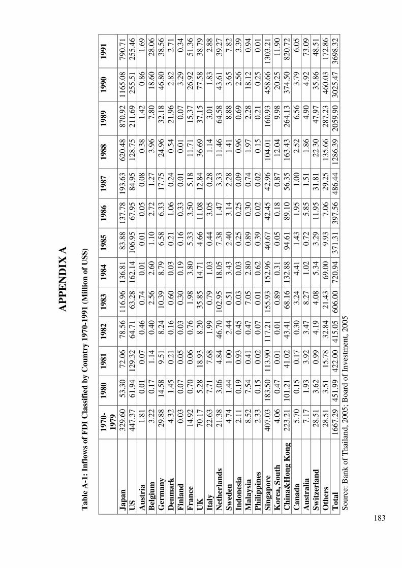
183
AP
PE
ND
IX A
T
ab
le A
-1:
Infl
ow
s of
FD
I C
lass
ifie
d b
y C
ou
ntr
y 1
970-1
991 (
Mil
lion
of
US
$)
1970-
1979
1980
1981
1982
1983
1984
1985
1986
1987
1988
1989
1990
1991
Jap
an
329.6
0
53.3
0
72.0
6
78.5
6
116.9
6
136.8
1
83.8
8
137.7
8
193.6
3
620.4
8
870.9
2
1165.0
8
790.7
1
US
447.3
7
61.9
4
129.3
2
64.7
1
63.2
8
162.1
4
106.9
5
67.9
5
84.9
5
128.7
5
211.6
9
255.5
1
255.4
6
Au
stri
a
1.8
1
0.0
1
0.0
7
0.4
6
0.7
4
0.0
1
0.0
1
0.0
5
0.0
8
0.3
8
1.4
2
0.8
6
1.6
9
Bel
giu
m
3.2
2
0.1
7
1.1
4
0.4
0
2.5
6
2.6
0
1.1
0
2.7
2
1.2
7
3.9
6
7.8
0
18.6
0
28.0
6
Ger
man
y
29.8
8
14.5
8
9.5
1
8.2
4
10.3
9
8.7
9
6.5
8
6.3
3
17.7
5
24.9
6
32.1
8
46.8
0
38.5
6
Den
mark
4.3
2
1.4
5
0.2
1
0.1
6
0.6
0
0.0
3
0.2
1
1.0
6
0.2
4
0.5
4
21.9
6
2.8
2
2.7
1
Fin
lan
d
0.0
3
0.0
7
0.0
5
0.0
3
0.3
0
0.1
9
0.1
6
0.3
3
0.0
1
0.0
1
0.0
7
3.2
9
0.3
4
Fra
nce
14.9
2
0.7
0
0.0
6
0.7
6
1.9
8
3.8
0
5.3
3
3.5
0
5.1
8
11.7
1
15.3
7
26.9
2
51.3
6
UK
70.1
7
5.2
8
18.9
3
8.2
0
35.8
5
14.7
1
4.6
6
11.0
8
12.8
4
36.6
9
37.1
5
77.5
8
38.7
9
Italy
22.6
3
7.7
1
7.6
8
1.9
9
0.7
9
1.0
3
0.4
4
3.0
5
0.2
8
1.1
4
3.0
1
1.8
3
2.8
8
Net
her
lan
ds
21.3
8
3.0
6
4.8
4
46.7
0
102.9
5
18.0
5
7.3
8
1.4
7
3.3
3
11.4
6
64.5
8
43.6
1
39.2
7
Sw
eden
4.7
4
1.4
4
1.0
0
2.4
4
0.5
1
3.4
3
2.4
0
3.1
4
2.2
8
1.4
1
8.8
8
3.6
5
7.8
2
Ind
on
esia
2.1
1
0.1
9
0.9
3
0.4
5
0.0
3
0.0
3
0.2
5
0.2
5
0.0
9
0.9
6
0.6
9
2.5
6
3.3
9
Mala
ysi
a
8.5
2
7.5
4
0.4
1
0.4
7
7.0
5
2.8
0
0.8
9
0.3
0
0.7
4
1.9
7
2.2
8
18.1
2
0.9
4
Ph
ilip
pin
es
2.3
3
0.1
5
0.0
2
0.0
7
0.0
1
0.6
2
0.3
9
0.0
2
0.0
2
0.1
5
0.2
1
0.2
5
0.0
1
Sin
gap
ore
407.0
3
183.5
0
113.9
0
117.2
1
155.9
3
152.9
6
40.6
7
42.4
5
42.9
6
104.0
1
160.9
3
458.6
6
1303.2
1
Kore
a, S
ou
th
4.0
6
0.4
7
0.0
1
0.0
1
0.8
9
0.3
1
0.0
5
0.1
8
0.8
7
12.0
4
9.9
8
20.2
5
11.9
0
Ch
ina&
Hon
g K
on
g
223.2
1
101.2
1
41.0
2
43.4
1
68.1
6
132.8
8
94.6
1
89.1
0
56.3
5
163.4
3
264.1
3
374.5
0
820.7
2
Can
ad
a
5.7
0
0.1
5
0.1
7
0.3
0
3.2
4
4.4
1
1.4
3
1.9
5
1.0
0
2.5
2
6.5
6
3.7
9
6.0
5
Au
stra
lia
7.1
7
1.9
3
3.9
2
3.4
7
8.2
7
1.0
2
0.7
2
5.8
5
1.5
1
1.8
6
4.9
0
4.9
2
73.0
9
Sw
itze
rlan
d
28.5
1
3.6
2
0.9
9
4.1
9
4.0
8
5.3
4
3.2
9
11.9
5
31.8
1
22.3
0
47.9
7
35.8
6
48.5
1
Oth
ers
28.5
1
3.5
1
15.7
8
32.8
4
21.4
3
69.0
0
9.9
3
7.0
6
29.2
5
135.6
6
287.2
3
460.0
3
172.8
6
Tota
l 1667.2
9
451.9
9
422.0
0
415.0
5
606.0
0
720.9
4
371.3
1
397.5
6
486.4
4
1286.3
9
2059.9
0
3025.4
7
3698.3
2
Sourc
e: B
ank o
f T
hai
lan
d, 2005;
Boar
d o
f In
ves
tmen
t, 2
005
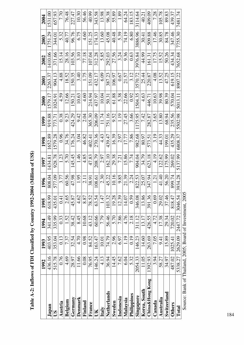
184
Tab
le A
-2:
Infl
ow
s of
FD
I C
lass
ifie
d b
y C
ou
ntr
y 1
992-2
004 (
Mil
lion
of
US
$)
1992
1993
1994
1995
1996
1997
1998
1999
2000
2001
2002
2003
2004
Jap
an
436.1
6
403.9
5
341.4
9
618.9
9
808.0
4
1434.8
1
1652.8
9
919.8
8
1579.1
7
2263.3
7
1410.0
6
1751.2
9
1531.0
0
US
515.7
8
353.0
4
335.9
9
435.0
1
577.0
9
928.7
8
1579.2
8
773.7
1
1024.9
1
904.1
3
371.6
6
344.0
1
657.9
3
Au
stri
a
0.7
6
0.1
3
0.3
3
0.4
1
3.7
7
1.2
3
0.9
6
0.3
8
4.5
9
4.8
8
15.1
4
5.3
2
7.7
0
Bel
giu
m
4.6
9
7.3
7
1.5
2
2.6
5
60.5
6
5.7
0
34.7
6
9.2
3
12.6
6
18.5
2
28.1
6
40.7
7
76.4
8
Ger
man
y
28.9
7
32.5
4
38.4
2
45.8
7
47.9
8
145.4
5
176.2
4
424.2
9
150.2
1
150.3
5
103.5
6
96.7
6
227.4
7
Den
mark
11.6
6
4.7
0
8.4
5
4.6
2
1.9
5
1.4
6
3.0
4
9.4
2
10.6
3
3.4
0
3.1
0
6.7
5
10.3
0
Fin
lan
d
0.0
8
0.9
8
10.6
8
8.8
7
2.1
1
4.8
5
46.8
2
2.0
4
4.6
0
1.7
5
77.1
8
4.6
0
56.4
6
Fra
nce
76.9
5
84.5
2
43.1
2
78.5
2
38.9
1
47.8
3
402.4
1
365.3
0
214.9
4
151.0
9
107.0
4
151.2
5
40.9
9
UK
146.2
4
163.4
7
60.6
6
63.5
4
108.6
1
208.7
9
270.3
6
206.0
9
437.9
7
432.1
7
312.2
8
174.3
3
343.5
8
Italy
4.1
3
10.0
1
7.7
9
1.4
7
2.3
0
2.9
7
4.4
3
11.7
4
10.0
4
6.0
9
5.8
5
13.6
0
13.9
8
Net
her
lan
ds
36.9
4
74.7
9
56.4
6
103.3
2
45.2
2
162.1
0
439.4
7
751.1
6
50.3
1
387.2
3
292.0
3
45.0
8
96.3
8
Sw
eden
14.4
5
2.9
6
5.7
0
19.2
8
10.1
6
29.3
8
16.3
9
9.5
2
61.8
8
106.9
7
27.5
6
40.4
8
55.8
9
Ind
on
esia
7.6
2
6.9
7
7.8
6
12.3
9
9.8
5
7.2
1
2.9
7
1.1
9
5.3
8
0.6
7
3.2
4
5.3
9
1.8
9
Mala
ysi
a
6.0
4
1.1
9
4.7
6
14.0
7
21.3
9
15.8
6
17.7
7
27.4
5
22.6
6
21.5
7
9.3
6
74.1
9
64.2
4
Ph
ilip
pin
es
5.3
2
0.1
9
2.1
8
0.5
9
2.2
4
7.7
4
7.8
6
3.6
6
0.9
2
3.1
2
0.6
3
6.8
0
183.1
5
Sin
gap
ore
2054.3
3
146.2
3
311.1
2
346.0
8
822.5
3
904.0
4
982.6
8
1175.9
5
1504.3
5
3570.7
2
3976.8
4
3886.9
6
3114.6
4
Kore
a, S
ou
th
11.0
5
14.6
0
13.1
7
13.8
6
25.0
7
34.7
9
80.9
7
7.4
2
4.6
3
25.4
4
44.9
9
30.4
1
40.2
1
Ch
ina&
Hon
g K
on
g
1392.9
3
263.6
9
426.5
5
391.3
6
347.9
4
623.1
8
573.5
1
282.8
7
446.7
1
220.8
7
161.3
1
509.8
8
409.0
9
Can
ad
a
3.9
4
7.0
5
4.7
2
0.6
9
1.2
1
4.1
9
3.1
9
3.6
5
10.6
3
4.0
8
17.7
5
17.4
6
7.2
8
Au
stra
lia
58.2
7
9.4
1
17.3
8
29.0
2
41.4
0
122.6
2
44.3
3
13.8
0
39.9
8
13.5
2
15.5
2
30.8
5
105.7
8
Sw
itze
rlan
d
34.9
7
15.8
9
29.3
4
37.4
6
56.2
0
175.9
9
199.0
1
68.9
4
80.3
9
47.2
5
50.2
6
84.7
8
89.8
3
Oth
ers
487.0
2
1025.4
1
720.0
2
818.4
7
899.7
4
269.0
2
435.2
9
235.5
6
570.0
4
619.1
5
434.3
4
347.4
6
439.3
7
Tota
l 5338.2
7
2629.0
9
2447.7
2
3046.5
4
3934.2
8
5137.9
9
6808.3
7
5502.9
8
5013.1
1
8907.2
2
7652.6
8
7755.3
0
7481.7
4
Sourc
e: B
ank o
f T
hai
lan
d, 2005;
Boar
d o
f In
ves
tmen
t, 2
005
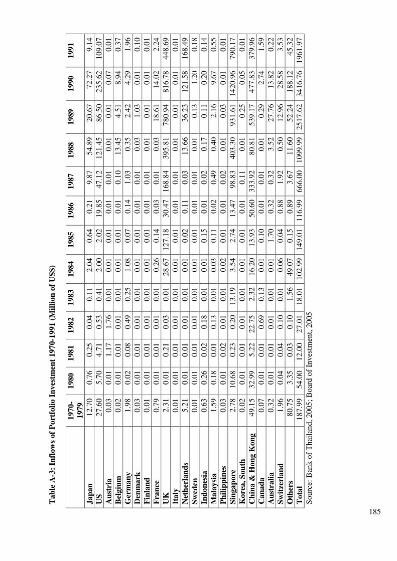
185
Tab
le A
-3:
Infl
ow
s of
Port
foli
o I
nves
tmen
t 197
0-1
991 (
Mil
lion
of
US
$)
1970-
1979
1980
1981
1982
1983
1984
1985
1986
1987
1988
1989
1990
1991
Jap
an
12.7
0
0.7
6
0.2
5
0.0
4
0.1
1
2.0
4
0.6
4
0.2
1
9.8
7
54.8
9
20.6
7
72.2
7
9.1
4
US
27.6
0
5.7
0
4.7
1
0.5
3
0.4
1
2.0
0
2.0
2
19.8
5
47.1
2
121.4
5
86.5
0
235.6
2
109.0
7
Au
stri
a
0.0
3
0.0
1
1.1
7
1.7
6
0.0
1
0.0
1
0.0
1
0.0
1
0.0
1
0.0
1
0.0
1
0.0
7
0.0
1
Bel
giu
m
0.0
2
0.0
1
0.0
1
0.0
1
0.0
1
0.0
1
0.0
1
0.0
1
0.1
0
13.4
5
4.5
1
8.9
4
0.3
7
Ger
man
y
1.9
8
0.0
2
0.0
8
0.4
9
0.2
5
1.0
8
0.0
7
0.1
4
1.0
3
0.3
5
2.4
2
4.2
9
1.9
6
Den
mark
0.0
3
0.0
1
0.0
1
0.0
1
0.0
1
0.0
1
0.0
1
0.0
1
0.0
1
0.0
3
1.0
3
0.0
1
0.1
0
Fin
lan
d
0.0
1
0.0
1
0.0
1
0.0
1
0.0
1
0.0
1
0.0
1
0.0
1
0.0
1
0.0
1
0.0
1
0.0
1
0.0
1
Fra
nce
0.7
9
0.0
1
0.0
1
0.0
1
0.0
1
0.2
6
0.1
4
0.0
3
0.0
1
0.0
3
18.6
1
14.0
2
2.2
4
UK
2.3
1
0.0
1
0.2
1
0.0
3
0.0
1
28.6
7
127.1
8
30.4
7
168.8
4
395.8
1
780.9
4
816.7
8
448.6
9
Italy
0.0
1
0.0
1
0.0
1
0.0
1
0.0
1
0.0
1
0.0
1
0.0
1
0.0
1
0.0
1
0.0
1
0.0
1
0.0
1
Net
her
lan
ds
5.2
1
0.0
1
0.0
1
0.0
1
0.0
1
0.0
1
0.0
2
0.1
1
0.0
3
13.6
6
36.2
3
121.5
8
168.4
9
Sw
eden
0.0
1
0.0
1
0.0
1
0.0
1
0.0
1
0.0
1
0.0
1
0.0
1
0.0
1
0.0
1
0.1
3
1.2
0
0.1
8
Ind
on
esia
0.6
3
0.2
6
0.0
2
0.1
8
0.0
1
0.0
1
0.1
5
0.0
1
0.0
2
0.1
7
0.1
1
0.2
0
0.1
4
Mala
ysi
a
1.5
9
0.1
8
0.0
1
0.1
3
0.0
1
0.0
3
0.1
1
0.0
2
0.4
9
0.4
0
2.1
6
9.6
7
0.5
5
Ph
ilip
pin
es
0.0
3
0.0
1
0.0
2
0.0
1
0.0
1
0.0
2
0.0
1
0.0
1
0.0
2
0.0
1
0.0
3
0.0
1
0.0
1
Sin
gap
ore
2.7
8
10.6
8
0.2
3
0.2
0
13.1
9
3.5
4
2.7
4
13.4
7
98.8
3
403.3
0
931.6
1
1420.9
6
790.1
7
Kore
a, S
ou
th
0.0
2
0.0
1
0.0
1
0.0
1
0.0
1
0.0
1
0.0
1
0.0
1
0.1
1
0.0
1
0.2
5
0.0
5
0.0
1
Ch
ina &
Hon
g K
on
g
49.1
5
32.9
9
5.2
2
22.7
5
2.3
2
16.2
0
13.9
3
50.6
0
333.9
2
80.8
1
539.1
7
477.8
3
379.9
6
Can
ad
a
0.0
7
0.0
1
0.0
1
0.6
9
0.1
3
0.0
1
0.1
0
0.0
1
0.0
1
0.0
1
0.2
9
2.7
4
1.5
9
Au
stra
lia
0.3
2
0.0
1
0.0
1
0.0
1
0.0
1
0.0
1
1.7
0
0.3
2
0.3
2
3.5
2
27.7
6
13.8
2
0.2
2
Sw
itze
rlan
d
1.9
6
0.0
4
0.0
4
0.1
0
0.0
1
0.0
6
0.0
4
0.8
8
1.9
2
0.5
0
12.9
6
28.5
8
3.5
3
Oth
ers
80.7
5
3.3
5
0.0
3
0.1
0
1.5
6
49.0
7
0.1
5
0.8
9
3.6
7
11.6
0
52.2
4
188.1
2
45.3
2
Tota
l 187.9
9
54.0
0
12.0
0
27.0
1
18.0
1
102.9
9
149.0
1
116.9
9
666.0
0
1099.9
9
2517.6
2
3416.7
6
1961.9
7
Sourc
e: B
ank o
f T
hai
lan
d, 2005;
Boar
d o
f In
ves
tmen
t, 2
005
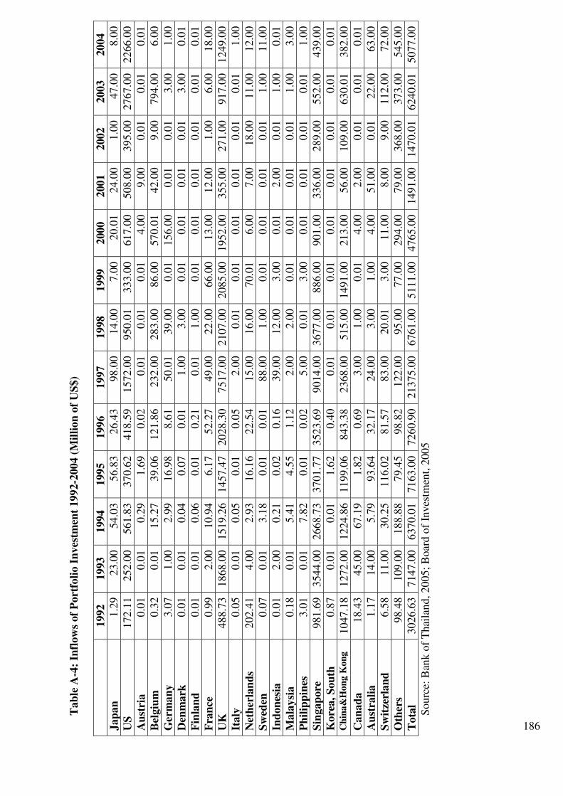
186
Tab
le A
-4:
Infl
ow
s of
Port
foli
o I
nves
tmen
t 199
2-2
004 (
Mil
lion
of
US
$)
1992
1993
1994
1995
1996
1997
1998
1999
2000
2001
2002
2003
2004
Jap
an
1.2
9
23.0
0
54.0
3
56.8
3
26.4
3
98.0
0
14.0
0
7.0
0
20.0
1
24.0
0
1.0
0
47.0
0
8.0
0
US
172.1
1
252.0
0
561.8
3
370.6
2
418.5
9
1572.0
0
950.0
1
333.0
0
617.0
0
508.0
0
395.0
0
2767.0
0
2266.0
0
Au
stri
a
0.0
1
0.0
1
0.2
9
1.6
9
0.0
2
0.0
1
0.0
1
0.0
1
4.0
0
9.0
0
0.0
1
0.0
1
0.0
1
Bel
giu
m
0.3
2
0.0
1
15.2
7
39.0
6
121.8
6
232.0
0
283.0
0
86.0
0
570.0
1
42.0
0
9.0
0
794.0
0
6.0
0
Ger
man
y
3.0
7
1.0
0
2.9
9
16.9
8
8.6
1
50.0
1
39.0
0
0.0
1
156.0
0
0.0
1
0.0
1
3.0
0
1.0
0
Den
mark
0.0
1
0.0
1
0.0
4
0.0
7
0.0
1
1.0
0
3.0
0
0.0
1
0.0
1
0.0
1
0.0
1
3.0
0
0.0
1
Fin
lan
d
0.0
1
0.0
1
0.0
6
0.0
1
0.2
1
0.0
1
1.0
0
0.0
1
0.0
1
0.0
1
0.0
1
0.0
1
0.0
1
Fra
nce
0.9
9
2.0
0
10.9
4
6.1
7
52.2
7
49.0
0
22.0
0
66.0
0
13.0
0
12.0
0
1.0
0
6.0
0
18.0
0
UK
488.7
3
1868.0
0
1519.2
6
1457.4
7
2028.3
0
7517.0
0
2107.0
0
2085.0
0
1952.0
0
355.0
0
271.0
0
917.0
0
1249.0
0
Italy
0.0
5
0.0
1
0.0
5
0.0
1
0.0
5
2.0
0
0.0
1
0.0
1
0.0
1
0.0
1
0.0
1
0.0
1
1.0
0
Net
her
lan
ds
202.4
1
4.0
0
2.9
3
16.1
6
22.5
4
15.0
0
16.0
0
70.0
1
6.0
0
7.0
0
18.0
0
11.0
0
12.0
0
Sw
eden
0.0
7
0.0
1
3.1
8
0.0
1
0.0
1
88.0
0
1.0
0
0.0
1
0.0
1
0.0
1
0.0
1
1.0
0
11.0
0
Ind
on
esia
0.0
1
2.0
0
0.2
1
0.0
2
0.1
6
39.0
0
12.0
0
3.0
0
0.0
1
2.0
0
0.0
1
1.0
0
0.0
1
Mala
ysi
a
0.1
8
0.0
1
5.4
1
4.5
5
1.1
2
2.0
0
2.0
0
0.0
1
0.0
1
0.0
1
0.0
1
1.0
0
3.0
0
Ph
ilip
pin
es
3.0
1
0.0
1
7.8
2
0.0
1
0.0
2
5.0
0
0.0
1
3.0
0
0.0
1
0.0
1
0.0
1
0.0
1
1.0
0
Sin
gap
ore
981.6
9
3544.0
0
2668.7
3
3701.7
7
3523.6
9
9014.0
0
3677.0
0
886.0
0
901.0
0
336.0
0
289.0
0
552.0
0
439.0
0
Kore
a, S
ou
th
0.8
7
0.0
1
0.0
1
1.6
2
0.4
0
0.0
1
0.0
1
0.0
1
0.0
1
0.0
1
0.0
1
0.0
1
0.0
1
Ch
ina
&H
on
g K
on
g
1047.1
8
1272.0
0
1224.8
6
1199.0
6
843.3
8
2368.0
0
515.0
0
1491.0
0
213.0
0
56.0
0
109.0
0
630.0
1
382.0
0
Can
ad
a
18.4
3
45.0
0
67.1
9
1.8
2
0.6
9
3.0
0
1.0
0
0.0
1
4.0
0
2.0
0
0.0
1
0.0
1
0.0
1
Au
stra
lia
1.1
7
14.0
0
5.7
9
93.6
4
32.1
7
24.0
0
3.0
0
1.0
0
4.0
0
51.0
0
0.0
1
22.0
0
63.0
0
Sw
itze
rlan
d
6.5
8
11.0
0
30.2
5
116.0
2
81.5
7
83.0
0
20.0
1
3.0
0
11.0
0
8.0
0
9.0
0
112.0
0
72.0
0
Oth
ers
98.4
8
109.0
0
188.8
8
79.4
5
98.8
2
122.0
0
95.0
0
77.0
0
294.0
0
79.0
0
368.0
0
373.0
0
545.0
0
Tota
l 3026.6
3
7147.0
0
6370.0
1
7163.0
0
7260.9
0
21375.0
0
6761.0
0
5111.0
0
4765.0
0
1491.0
0
1470.0
1
6240.0
1
5077.0
0
Sourc
e: B
ank o
f T
hai
lan
d, 2005;
Boar
d o
f In
ves
tmen
t, 2
005
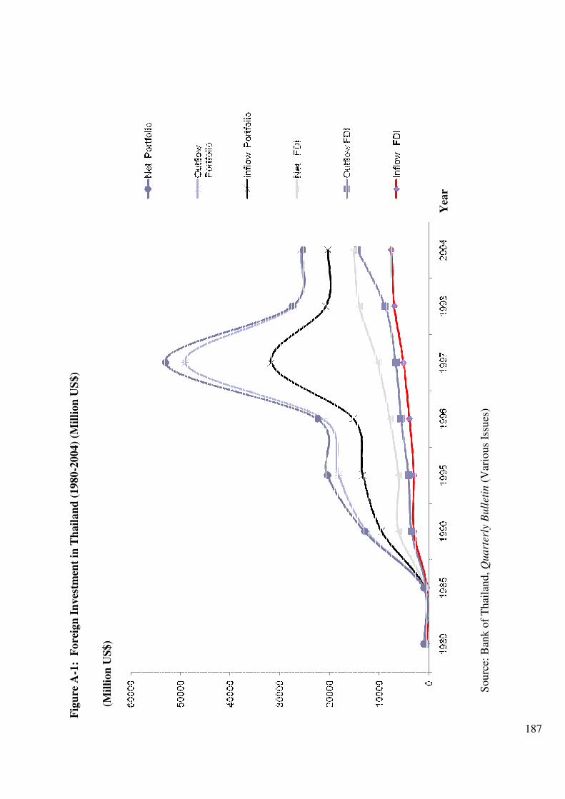
187
Fig
ure
A-1
: F
ore
ign
In
ves
tmen
t in
Th
ail
an
d (
1980-2
004)
(Mil
lion
US
$)
(M
illi
on
US
$)
Sourc
e: B
ank o
f T
hai
lan
d, Q
uart
erly
Bull
etin
(V
ario
us
Issu
es)
Yea
r
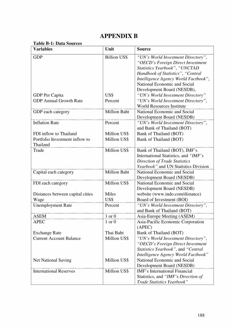
188
APPENDIX B Table B-1: Data Sources
Variables Unit Source
GDP Billion US$ “UN’s World Investment Directory”, “OECD’s Foreign Direct Investment
Statistics Yearbook”, “UNCTAD
Handbook of Statistics”, “Central
Intelligence Agency World Factbook”, National Economic and Social Development Board (NESDB),
GDP Per Capita US$ “UN’s World Investment Directory”
GDP Annual Growth Rate Percent “UN’s World Investment Directory”, World Resources Institute
GDP each category Million Baht National Economic and Social Development Board (NESDB)
Inflation Rate Percent “UN’s World Investment Directory”, and Bank of Thailand (BOT)
FDI inflow to Thailand Million US$ Bank of Thailand (BOT)
Portfolio Investment inflow to Thailand
Million US$ Bank of Thailand (BOT)
Trade Million US$ Bank of Thailand (BOT), IMF’s International Statistics, and “IMF’s
Direction of Trade Statistics
Yearbook” and UN Statistics Division
Capital each category Million Baht National Economic and Social Development Board (NESDB)
FDI each category Million US$ National Economic and Social Development Board (NESDB)
Distances between capital cities Miles website (www.indo.com/distance)
Wage US$ Board of Investment (BOI)
Unemployment Rate Percent “UN’s World Investment Directory”, and Bank of Thailand (BOT)
ASEM 1 or 0 Asia-Europe Meeting (ASEM)
APEC 1 or 0 Asia-Pacific Economic Corporation (APEC)
Exchange Rate Thai Baht Bank of Thailand (BOT)
Current Account Balance Million US$ “UN’s World Investment Directory”, “OECD’s Foreign Direct Investment
Statistics Yearbook”, and “Central
Intelligence Agency World Factbook”
Net National Saving Million US$ National Economic and Social Development Board (NESDB)
International Reserves Million US$ IMF’s International Financial Statistics, and “IMF’s Direction of
Trade Statistics Yearbook”
189
Table B-2: Data Description
Variable Descriptive GDP based on GDP in national currency and the exchange
rate projections provided by the country
GDP Per Capita converting GDP in local currencies to US Dollars and then dividing GDP by the total population
GDP Annual Growth Rate a different between a current year of GDP and the GDP previous year in percentage
GDP each category GDP in each industrial category
Inflation Rate annual percentage change averages for the year, not end-of-period
FDI Inflow to Thailand total amount of inflows from 21 investing partners into Thailand
Portfolio Investment inflow to Thailand
total of transaction involving in equity securities, debt securities in the forms of bonds, notes, money market instrument and financial derivatives from 21 investing partners to Thailand
Trade total amount of imports and exports between investing partner i and Thailand in US Dollar
Capital each category net capital stock in each industrial category
FDI each category FDI in each industrial category
Distances between capital cities geographic distance between capitals of investing partner i and Bangkok, Thailand
Wage (in Equations (5.5), (5.6), (5.10), and (5.11))
the minimum wage rate per day in each investing partner
Wage (in Equation (5.16)) the minimum wage rate per day in Thailand
Unemployment Rate age 15 years and over but do not work or have no permanent job
ASEM and APEC memberships of both investing partner i and Thailand
Exchange Rate (in Equations (5.5), (5.6), (5.10), and (5.11))
a ratio of Thai Baht and investing partner i’s currency
Exchange Rate Thai Baht per US Dollar
Current Account Balance sum of trade balance, service and transfer account, and current transfer
Net National Saving total national saving of Thailand
International Reserves foreign assets held or controlled by the BOT which consists of monetary gold, special drawing rights, reserve positions in the Fund, and foreign exchange assets
190
Table B-3: Descriptive Statistics for Variables Used in the Extended Gravity Models
Variable Mean Std.dev. Minimum Maximum
Endowment variables
Log of FDI Inflow LnFDIit 2.09 3.17 -13.82 8.29
Log of Portfolio
Investment Inflow
LnPRTit -3.75 7.66 -13.82 9.11
Log of Exchange Rate LnXit 1.31 2.10 -4.27 6.16
Log of GDP Ln(GDPit*GDPt) 10.17 1.66 5.95 14.47
Log of GDP Per Capita Ln(CAPit*CAPt) 16.53 1.51 12.24 18.68
GDP Growth Rate GDPGRit 3.39 3.31 -13.10 15.20
Log of Trade LnTRADEit 7.09 2.43 1.14 22.51
Inflation Rate INFLit 4.56 5.15 -1.00 58.00
Log of Wage Rate LnWGEit 6.26 3.10 0.20 16.60
Log of Distance LnDISit 8.21 0.70 6.61 9.08
Dummy variables
APEC APECit 0.33 0.47 0.00 1.00
ASEM ASEMit 0.31 0.46 0.00 1.00
Note: The number of observations is 525.
191
Table B-4: Descriptive Statistics for Variables Used in the Determinants of FDI into Thailand by Categories
Variable Mean Std.dev. Minimum Maximum
Endowment variables Log of FDI in Industry 8.41 1.18 6.13 11.18 Log of FDI in Financial Institutions 9.89 1.52 7.04 12.08 Log of FDI in Trade 9.31 1.70 6.67 12.00 Log of FDI in Construction 7.69 0.84 6.36 9.60 Log of FDI in Mining and Quarrying 7.60 1.26 5.61 11.34 Log of FDI in Agricultural Products 4.81 1.35 2.01 6.98 Log of FDI in Services 7.91 1.46 5.79 10.54 Log of FDI in Investment 2.16 6.72 -4.61 10.12 Log of FDI in Real Estate 7.74 1.82 4.67 10.00 Log of FDI in Others 2.56 7.02 -6.91 10.37 Log of GDP in Industry 13.40 0.91 11.87 14.62 Log of GDP in Financial Institutions 11.54 0.94 9.93 12.76 Log of GDP in Trade 12.90 0.70 11.67 13.80 Log of GDP in Construction 11.66 0.74 10.29 12.74 Log of GDP in Mining and Quarrying 10.66 0.84 9.32 12.07 Log of GDP in Agricultural Products 12.57 0.41 11.94 13.21 Log of GDP in Services 12.69 0.72 11.44 13.63 Log of GDP in Investment 11.35 0.78 10.03 12.60 Log of GDP in Real Estate 11.40 0.61 10.33 12.15 Log of GDP in Others 12.00 0.79 10.46 13.00 Log of Capital in Industry 13.71 1.12 11.90 15.13 Log of Capital in Financial Institutions 11.60 0.62 10.64 12.47 Log of Capital in Trade 13.38 0.62 12.44 14.23 Log of Capital in Construction 12.01 1.20 10.05 13.49 Log of Capital in Mining and Quarrying 11.26 1.01 9.40 12.56 Log of Capital in Agricultural Products 13.12 0.65 12.15 14.12 Log of Capital in Services 13.47 0.81 12.15 14.53 Log of Capital in Investment 14.26 0.96 12.70 15.60 Log of Capital in Real Estate 14.18 0.94 12.44 15.27 Log of Capital in Others 11.50 0.95 9.83 12.75 Inflation Rate 4.63 4.14 0.30 19.70 Log of Exchange Rate 3.36 .25 3.03 3.80 Log of International Reserves 12.85 1.29 10.98 14.51 Current Account Balance (Baht) 32184.89 245664.78 -364320.00 591606.00 Log of Net National Saving 12.96 0.92 10.80 13.94 Log of Wage 10.57 0.41 9.89 11.06 Unemployment Rate 2.88 0.76 1.55 4.50 Dummy variables APEC 0.64 0.49 0 1 ASEM 0.36 0.49 0 1
Note: The number of observations is 25.
192
APPENDIX C Table C-1: Comparison of FEM and REM for Models 1 and 2 of the Determinants of
Portfolio Investment in Thailand Using Equation (5.6)
Variable Coefficients
Model 1 a 1 b 2 c 2 d
GDP -8.0049*** .6114 -7.9135*** .7706
GDP Per Capita 11.9400*** 1.9179*** 11.8131*** 1.6535***
GDP Growth Rate .0694 .1021 .1216 .1743*
Distance -8.0795 -2.2991 -8.1476 -2.3023*
Trade - - .1906 .2132
Exchange Rate - - .2418 1.1070***
Wage Rate - - -.0258 .0126
Inflation Rate - - .0781 .1104*
APEC - - - -
ASEM - - - -
Constant - -23.1334* - -21.1535**
No. of observations 525 525 525 525
Mean -3.7513 -3.7513 -3.7513 -3.7513
Std. Dev. 4.9906 7.6612 4.9918 7.6613
Sum of squares 12453.16 14260.51 12359.28 12673.72
R2 59.47% 52.27% 59.78% 57.58%
Adjusted R2 57.53% 51.89% 57.51% 56.90%
F-Statistics 30.57*** 12.80*** 26.33*** 10.17***
Hausman-test 15.56*** 15.56 21.48*** 21.48
FEM REM FEM REM
Notes: i. ***, **, and * represent statistical significance at the 1%, 5% and 10% levels, respectively.
ii. FEM is the fixed effects model. iii. REM is the random effects model. iv. 1a and 1b Models represent the basic specification of extended Gravity Model
which include GDP, GDP Per Capita, GDP Growth Rate, and Distance. v. 2c and 2d Models represent the basic specification variables, the
macroeconomic variables of the investing partners (Wage Rate and Inflation Rate) and the economic relationship variables between Thailand and investing partners (Trade and Exchange Rate).
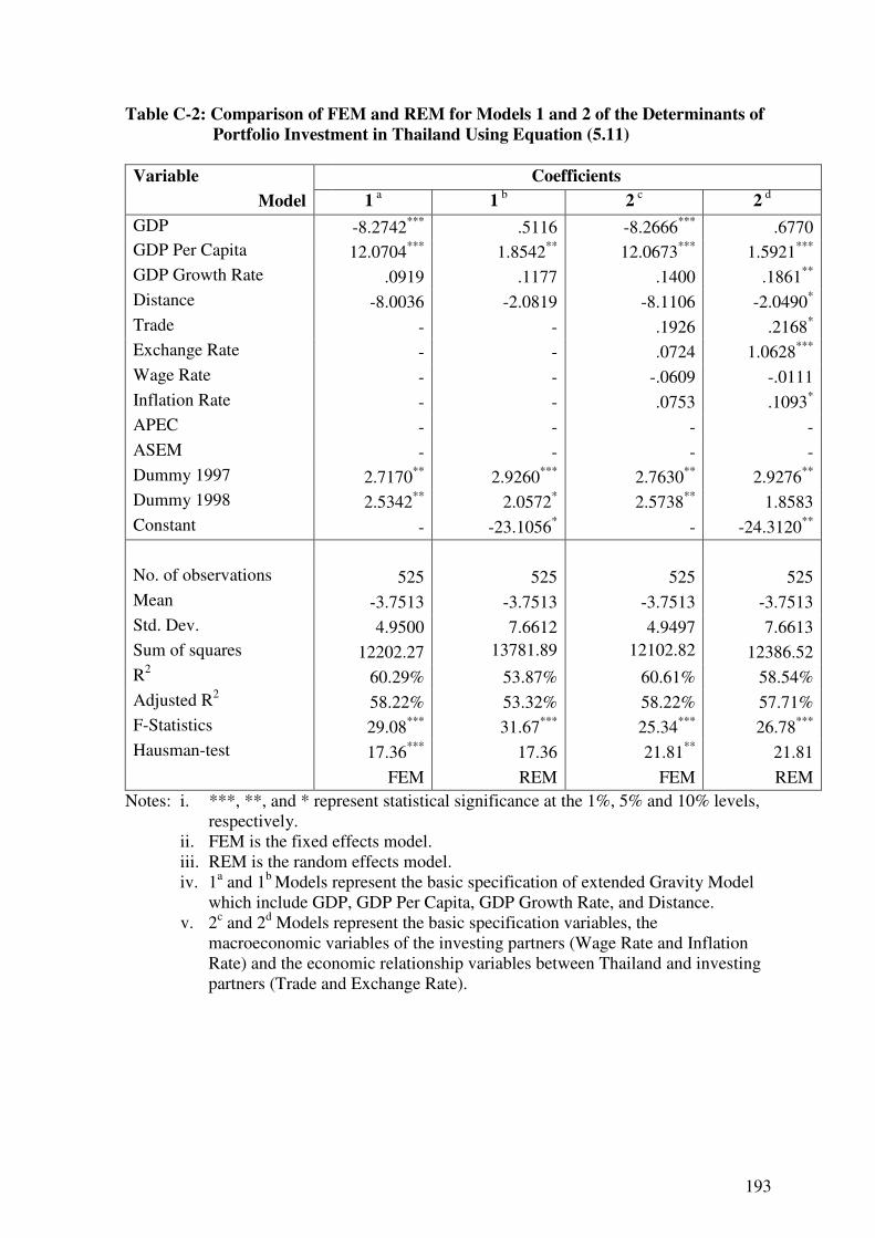
193
Table C-2: Comparison of FEM and REM for Models 1 and 2 of the Determinants of Portfolio Investment in Thailand Using Equation (5.11)
Variable Coefficients
Model 1 a 1 b 2 c 2 d
GDP -8.2742*** .5116 -8.2666*** .6770
GDP Per Capita 12.0704*** 1.8542** 12.0673*** 1.5921***
GDP Growth Rate .0919 .1177 .1400 .1861**
Distance -8.0036 -2.0819 -8.1106 -2.0490*
Trade - - .1926 .2168*
Exchange Rate - - .0724 1.0628***
Wage Rate - - -.0609 -.0111
Inflation Rate - - .0753 .1093*
APEC - - - -
ASEM - - - -
Dummy 1997 2.7170** 2.9260*** 2.7630** 2.9276**
Dummy 1998 2.5342** 2.0572* 2.5738** 1.8583
Constant - -23.1056* - -24.3120**
No. of observations 525 525 525 525
Mean -3.7513 -3.7513 -3.7513 -3.7513
Std. Dev. 4.9500 7.6612 4.9497 7.6613
Sum of squares 12202.27 13781.89 12102.82 12386.52
R2 60.29% 53.87% 60.61% 58.54%
Adjusted R2 58.22% 53.32% 58.22% 57.71%
F-Statistics 29.08*** 31.67*** 25.34*** 26.78***
Hausman-test 17.36*** 17.36 21.81** 21.81
FEM REM FEM REM
Notes: i. ***, **, and * represent statistical significance at the 1%, 5% and 10% levels, respectively.
ii. FEM is the fixed effects model. iii. REM is the random effects model. iv. 1a and 1b Models represent the basic specification of extended Gravity Model
which include GDP, GDP Per Capita, GDP Growth Rate, and Distance. v. 2c and 2d Models represent the basic specification variables, the
macroeconomic variables of the investing partners (Wage Rate and Inflation Rate) and the economic relationship variables between Thailand and investing partners (Trade and Exchange Rate).
194
APPENDIX D Table D-1: List of Variables
Variable Definition
LFDI Log of FDI
LPRT Log of Portfolio Investment
LGG Log of GDP
LCC Log of GDP Per Capita
GDPGR GDP Growth Rate
LDIS Log of Distance
LTRA Log of Trade
LX Log of Exchange Rate
WAGE Wage Rate
INFL Inflation Rate
ASEM ASEM
APEC APEC
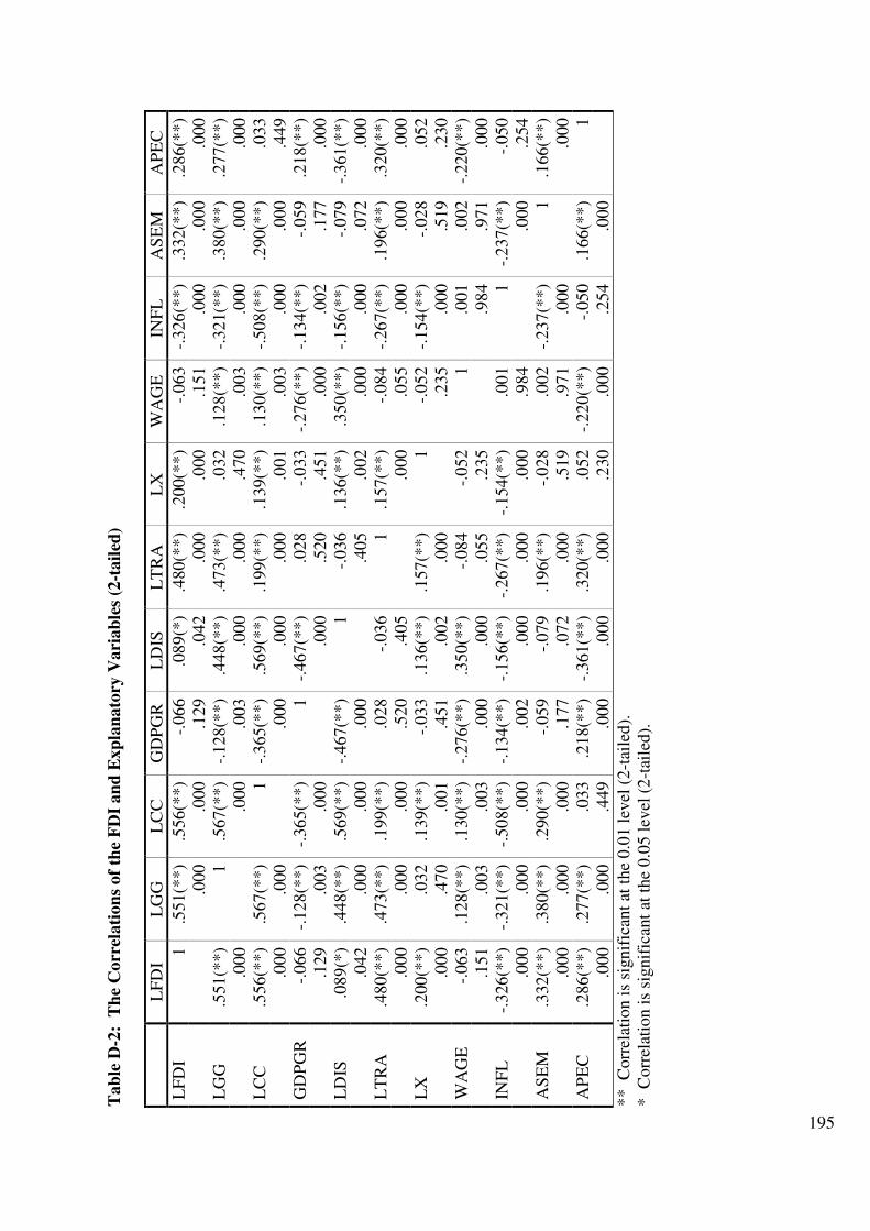
195
Tab
le D
-2:
Th
e C
orr
elati
on
s of
the
FD
I an
d E
xp
lan
ato
ry V
ari
ab
les
(2-t
ail
ed)
L
FD
I L
GG
L
CC
G
DP
GR
L
DIS
L
TR
A
LX
W
AG
E
INF
L
AS
EM
A
PE
C
LF
DI
1
.551(*
*)
.556(*
*)
-.066
.089(*
) .4
80(*
*)
.200(*
*)
-.063
-.326(*
*)
.332(*
*)
.286(*
*)
.000
.000
.129
.042
.000
.000
.151
.000
.000
.000
LG
G
.551(*
*)
1
.567(*
*)
-.128(*
*)
.448(*
*)
.473(*
*)
.032
.128(*
*)
-.321(*
*)
.380(*
*)
.277(*
*)
.0
00
.0
00
.003
.000
.000
.470
.003
.000
.000
.000
LC
C
.556(*
*)
.567(*
*)
1
-.365(*
*)
.569(*
*)
.199(*
*)
.139(*
*)
.130(*
*)
-.508(*
*)
.290(*
*)
.033
.0
00
.000
.0
00
.000
.000
.001
.003
.000
.000
.449
GD
PG
R
-.066
-.128(*
*)
-.365(*
*)
1
-.467(*
*)
.028
-.033
-.276(*
*)
-.134(*
*)
-.059
.218(*
*)
.1
29
.003
.000
.0
00
.520
.451
.000
.002
.177
.000
LD
IS
.089(*
) .4
48(*
*)
.569(*
*)
-.467(*
*)
1
-.036
.136(*
*)
.350(*
*)
-.156(*
*)
-.079
-.361(*
*)
.0
42
.000
.000
.000
.4
05
.002
.000
.000
.072
.000
LT
RA
.4
80(*
*)
.473(*
*)
.199(*
*)
.028
-.036
1
.157(*
*)
-.084
-.267(*
*)
.196(*
*)
.320(*
*)
.0
00
.000
.000
.520
.405
.0
00
.055
.000
.000
.000
LX
.2
00(*
*)
.032
.139(*
*)
-.033
.136(*
*)
.157(*
*)
1
-.052
-.154(*
*)
-.028
.052
.0
00
.470
.001
.451
.002
.000
.2
35
.000
.519
.230
WA
GE
-.
063
.128(*
*)
.130(*
*)
-.276(*
*)
.350(*
*)
-.084
-.052
1
.001
.002
-.220(*
*)
.1
51
.003
.003
.000
.000
.055
.235
.9
84
.971
.000
INF
L
-.326(*
*)
-.321(*
*)
-.508(*
*)
-.134(*
*)
-.156(*
*)
-.267(*
*)
-.154(*
*)
.001
1
-.237(*
*)
-.050
.0
00
.000
.000
.002
.000
.000
.000
.984
.0
00
.254
AS
EM
.3
32(*
*)
.380(*
*)
.290(*
*)
-.059
-.079
.196(*
*)
-.028
.002
-.237(*
*)
1
.166(*
*)
.0
00
.000
.000
.177
.072
.000
.519
.971
.000
.0
00
AP
EC
.2
86(*
*)
.277(*
*)
.033
.218(*
*)
-.361(*
*)
.320(*
*)
.052
-.220(*
*)
-.050
.166(*
*)
1
.0
00
.000
.449
.000
.000
.000
.230
.000
.254
.000
** C
orr
elat
ion i
s si
gnif
ican
t at
the
0.0
1 l
evel
(2
-tai
led).
* C
orr
elat
ion i
s si
gnif
ican
t at
the
0.0
5 l
evel
(2-t
aile
d).

196
Tab
le D
-3:
Th
e C
orr
elati
on
s of
the
Fore
ign
Po
rtfo
lio I
nves
tmen
t an
d E
xp
lan
ato
ry V
ari
ab
les
(2-t
ail
ed)
L
PR
T
LG
G
LC
C
GD
PG
R
LD
IS
LT
RA
L
X
WA
GE
IN
FL
A
SE
M
AP
EC
LP
RT
1
.389(*
*)
.355(*
*)
-.019
.042
.382(*
*)
.383(*
*)
-.070
-.232(*
*)
.080
.224(*
*)
.000
.000
.663
.334
.000
.000
.111
.000
.066
.000
LG
G
.389(*
*)
1
.567(*
*)
-.128(*
*)
.448(*
*)
.473(*
*)
.032
.128(*
*)
-.321(*
*)
.380(*
*)
.277(*
*)
.0
00
.0
00
.003
.000
.000
.470
.003
.000
.000
.000
LC
C
.355(*
*)
.567(*
*)
1
-.365(*
*)
.569(*
*)
.199(*
*)
.139(*
*)
.130(*
*)
-.508(*
*)
.290(*
*)
.033
.0
00
.000
.0
00
.000
.000
.001
.003
.000
.000
.449
GD
PG
R
-.019
-.128(*
*)
-.365(*
*)
1
-.467(*
*)
.028
-.033
-.276(*
*)
-.134(*
*)
-.059
.218(*
*)
.6
63
.003
.000
.0
00
.520
.451
.000
.002
.177
.000
LD
IS
.042
.448(*
*)
.569(*
*)
-.467(*
*)
1
-.036
.136(*
*)
.350(*
*)
-.156(*
*)
-.079
-.361(*
*)
.3
34
.000
.000
.000
.4
05
.002
.000
.000
.072
.000
LT
RA
.3
82(*
*)
.473(*
*)
.199(*
*)
.028
-.036
1
.157(*
*)
-.084
-.267(*
*)
.196(*
*)
.320(*
*)
.0
00
.000
.000
.520
.405
.0
00
.055
.000
.000
.000
LX
.3
83(*
*)
.032
.139(*
*)
-.033
.136(*
*)
.157(*
*)
1
-.052
-.154(*
*)
-.028
.052
.0
00
.470
.001
.451
.002
.000
.2
35
.000
.519
.230
WA
GE
-.
070
.128(*
*)
.130(*
*)
-.276(*
*)
.350(*
*)
-.084
-.052
1
.001
.002
-.220(*
*)
.1
11
.003
.003
.000
.000
.055
.235
.9
84
.971
.000
INF
L
-.232(*
*)
-.321(*
*)
-.508(*
*)
-.134(*
*)
-.156(*
*)
-.267(*
*)
-.154(*
*)
.001
1
-.237(*
*)
-.050
.0
00
.000
.000
.002
.000
.000
.000
.984
.0
00
.254
AS
EM
.0
80
.380(*
*)
.290(*
*)
-.059
-.079
.196(*
*)
-.028
.002
-.237(*
*)
1
.166(*
*)
.0
66
.000
.000
.177
.072
.000
.519
.971
.000
.0
00
AP
EC
.2
24(*
*)
.277(*
*)
.033
.218(*
*)
-.361(*
*)
.320(*
*)
.052
-.220(*
*)
-.050
.166(*
*)
1
.0
00
.000
.449
.000
.000
.000
.230
.000
.254
.000
** C
orr
elat
ion i
s si
gnif
ican
t at
the
0.0
1 l
evel
(2
-tai
led).
197
AP
PE
ND
IX E
T
ab
le E
-1:
Au
stra
lia
Yea
r F
DI1
P
RT
2
TR
D3
X4
CA
P5
GD
PG
R6
GD
P
INF
L7
DIS
8
AS
EM
A
PE
C
D97
9
D98
10
Note
1980
1.9
3
0.0
1
243.1
2
24.8
2
10628.8
8
3.3
0
156.2
4
9.0
0
4647
0
0
0
0
1 =
FD
I
1981
3.9
2
0.0
1
274.3
9
25.2
9
12072.1
0
3.1
0
180.1
2
9.5
0
4647
0
0
0
0
outf
low
to
1982
3.4
7
0.0
1
262.8
7
23.6
2
11758.2
7
-2.4
0
178.4
9
10.4
0
4647
0
0
0
0
Thai
land
1983
8.2
7
0.0
1
279.4
4
20.9
6
11117.8
7
4.8
0
171.1
0
8.6
0
4647
0
0
0
0
2 =
Port
foli
o
1984
1.0
2
0.0
1
319.6
0
20.9
5
12115.5
0
5.3
0
188.5
2
5.9
0
4647
0
0
0
0
Outf
low
to
1985
0.7
2
1.7
0
277.0
0
19.2
3
10588.9
0
4.3
0
167.2
0
7.0
0
4647
0
0
0
0
Thai
land
1986
5.8
5
0.3
2
318.8
4
17.8
0
10818.4
1
2.3
0
173.3
1
9.7
0
4647
0
0
0
0
3 =
Tra
de
1987
1.5
1
0.3
2
442.7
1
18.1
8
12547.5
8
5.4
0
204.0
2
8.5
0
4647
0
0
0
0
wit
h
1988
1.8
6
3.5
2
645.2
5
19.9
7
15660.6
2
4.0
0
259.5
9
4.6
0
4647
0
0
0
0
Thai
land
1989
4.9
0
27.7
6
888.9
5
20.5
0
17425.0
3
3.7
0
293.5
6
7.5
0
4647
0
1
0
0
4 =
Ex
chan
ge
1990
4.9
2
13.8
2
933.2
8
20.1
2
18011.3
1
-0.1
0
307.8
2
7.3
0
4647
0
1
0
0
Rat
e
1991
73.0
9
0.2
2
1124.8
0
20.0
1
18016.3
6
0.3
0
311.9
1
3.2
0
4647
0
1
0
0
5 =
GD
P
1992
58.2
7
1.1
7
1438.1
3
18.4
0
17413.9
6
3.7
0
305.0
6
1.0
0
4647
0
1
0
0
Per
cap
ita
1993
9.4
1
14.0
0
1463.8
2
17.3
5
16747.3
6
3.9
0
296.3
7
1.8
0
4647
0
1
0
0
6 =
GD
P
1994
17.3
8
5.7
9
1721.5
0
18.5
3
18815.0
3
4.2
0
336.4
9
1.9
0
4647
0
1
0
0
Gro
wth
rat
e
1995
29.0
2
93.6
4
2099.9
1
18.6
0
19814.5
3
4.2
0
358.7
2
4.6
0
4647
0
1
0
0
7 =
Infl
atio
n
1996
41.4
0
32.1
7
2244.0
7
19.9
7
22001.4
4
3.8
0
403.4
9
2.6
0
4647
0
1
0
0
Rat
e
1997
122.6
2
24.0
0
2243.2
3
23.3
0
21816.2
2
4.5
0
404.5
5
0.3
0
4647
0
1
1
0
8 =
Dis
tance
1998
44.3
3
3.0
0
1865.9
3
26.3
9
19324.7
3
5.3
0
362.1
6
0.9
0
4647
0
1
0
1
to T
hai
land
1999
13.8
0
1.0
0
2286.1
5
24.6
6
20546.8
9
4.0
0
389.5
2
1.5
0
4647
0
1
0
0
9 =
1997
2000
39.9
8
4.0
0
2800.4
3
23.5
4
19669.2
9
1.8
0
377.4
0
4.5
0
4647
0
1
0
0
10 =
1998
2001
13.5
2
51.0
0
2708.5
1
23.2
5
18389.9
1
3.9
0
357.5
6
4.4
0
4647
0
1
0
0
2002
15.5
2
0.0
1
3135.6
2
23.3
5
20355.9
3
2.7
0
400.4
5
3.0
0
4647
0
1
0
0
2003
30.8
5
22.0
0
3727.9
7
27.0
0
25683.0
5
2.4
0
511.2
8
2.8
0
4647
0
1
0
0
2004
105.7
8
63.0
0
4665.6
0
29.6
0
30681.7
9
3.4
0
618.0
2
2.3
0
4647
0
1
0
0
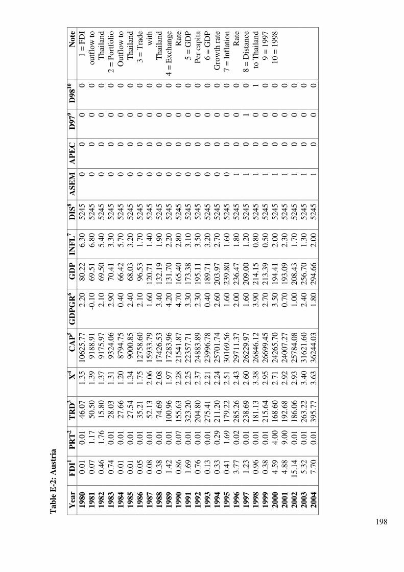
198
Tab
le E
-2:
Au
stri
a
Yea
r F
DI1
P
RT
2
TR
D3
X4
CA
P5
GD
PG
R6
GD
P
INF
L7
DIS
8
AS
EM
A
PE
C
D97
9
D98
10
Note
1980
0.0
1
0.0
1
46.0
7
1.3
5
10625.7
7
2.2
0
80.2
2
6.3
0
5245
0
0
0
0
1 =
FD
I
1981
0.0
7
1.1
7
50.5
0
1.3
9
9188.9
1
-0.1
0
69.5
1
6.8
0
5245
0
0
0
0
outf
low
to
1982
0.4
6
1.7
6
15.8
0
1.3
7
9175.9
7
2.1
0
69.5
0
5.4
0
5245
0
0
0
0
Thai
land
1983
0.7
4
0.0
1
28.0
3
1.3
1
9324.0
6
2.9
0
70.4
1
3.3
0
5245
0
0
0
0
2 =
Port
foli
o
1984
0.0
1
0.0
1
27.6
6
1.2
0
8794.7
5
0.4
0
66.4
2
5.7
0
5245
0
0
0
0
Outf
low
to
1985
0.0
1
0.0
1
27.5
4
1.3
4
9000.8
5
2.4
0
68.0
3
3.2
0
5245
0
0
0
0
Thai
land
1986
0.0
5
0.0
1
35.2
1
1.7
5
12758.6
0
2.1
0
96.5
3
1.7
0
5245
0
0
0
0
3 =
Tra
de
1987
0.0
8
0.0
1
52.1
3
2.0
6
15933.7
9
1.6
0
120.7
1
1.4
0
5245
0
0
0
0
wit
h
1988
0.3
8
0.0
1
74.6
9
2.0
8
17426.5
3
3.4
0
132.1
9
1.9
0
5245
0
0
0
0
Thai
land
1989
1.4
2
0.0
1
100.9
6
1.9
7
17283.9
6
4.2
0
131.7
0
2.2
0
5245
0
0
0
0
4 =
Ex
chan
ge
1990
0.8
6
0.0
7
155.6
3
2.2
8
21541.8
7
4.7
0
165.4
0
2.8
0
5245
0
0
0
0
Rat
e
1991
1.6
9
0.0
1
323.2
0
2.2
5
22357.7
1
3.3
0
173.3
8
3.1
0
5245
0
0
0
0
5 =
GD
P
1992
0.7
6
0.0
1
204.8
0
2.3
7
24883.8
9
2.3
0
195.1
1
3.5
0
5245
0
0
0
0
Per
cap
ita
1993
0.1
3
0.0
1
275.4
1
2.2
1
23996.7
8
0.4
0
189.7
1
3.2
0
5245
0
0
0
0
6 =
GD
P
1994
0.3
3
0.2
9
211.2
0
2.2
4
25701.7
4
2.6
0
203.9
7
2.7
0
5245
0
0
0
0
Gro
wth
rat
e
1995
0.4
1
1.6
9
179.2
2
2.5
1
30169.5
6
1.6
0
239.8
0
1.6
0
5245
0
0
0
0
7 =
Infl
atio
n
1996
3.7
7
0.0
2
285.2
6
2.4
3
29711.3
7
2.0
0
236.4
7
1.8
0
5245
1
0
0
0
Rat
e
1997
1.2
3
0.0
1
238.6
9
2.6
0
26229.9
7
1.6
0
209.0
0
1.2
0
5245
1
0
1
0
8 =
Dis
tance
1998
0.9
6
0.0
1
181.1
3
3.3
8
26846.1
2
3.9
0
214.1
5
0.8
0
5245
1
0
0
1
to T
hai
land
1999
0.3
8
0.0
1
215.6
4
2.9
5
26699.4
5
2.7
0
213.3
9
0.5
0
5245
1
0
0
0
9 =
1997
2000
4.5
9
4.0
0
168.6
0
2.7
1
24265.7
0
3.5
0
194.4
1
2.0
0
5245
1
0
0
0
10 =
1998
2001
4.8
8
9.0
0
192.6
8
2.9
2
24007.2
7
0.7
0
193.0
9
2.3
0
5245
1
0
0
0
2002
15.1
4
0.0
1
186.0
6
2.9
3
25784.0
8
1.0
0
208.4
3
1.7
0
5245
1
0
0
0
2003
5.3
2
0.0
1
263.2
2
3.4
0
31621.6
0
2.4
0
256.7
0
1.3
0
5245
1
0
0
0
2004
7.7
0
0.0
1
395.7
7
3.6
3
36244.0
3
1.8
0
294.6
6
2.0
0
5245
1
0
0
0

199
Tab
le E
-3:
Bel
giu
m
Yea
r F
DI1
P
RT
2
TR
D3
X4
CA
P5
GD
PG
R6
GD
P
INF
L7
DIS
8
AS
EM
A
PE
C
D97
9
D98
10
Note
1980
0.1
7
0.0
1
213.3
5
0.5
6
12332.2
0
4.5
0
121.5
6
6.7
0
5479
0
0
0
0
1 =
FD
I
1981
1.1
4
0.0
1
164.2
9
0.5
9
10248.7
8
-0.3
0
101.0
8
7.6
0
5479
0
0
0
0
outf
low
to
1982
0.4
0
0.0
1
138.9
2
0.5
1
9013.9
2
0.6
0
88.9
3
8.7
0
5479
0
0
0
0
Thai
land
1983
2.5
6
0.0
1
184.8
4
0.4
6
8528.1
8
0.3
0
84.1
3
7.7
0
5479
0
0
0
0
2 =
Port
foli
o
1984
2.6
0
0.0
1
174.6
9
0.4
2
8121.2
4
2.5
0
80.1
2
6.4
0
5479
0
0
0
0
Outf
low
to
1985
1.1
0
0.0
1
165.4
0
0.4
7
8454.4
2
1.7
0
83.4
3
4.9
0
5479
0
0
0
0
Thai
land
1986
2.7
2
0.0
1
198.4
3
0.5
9
11715.2
5
1.8
0
115.6
5
1.3
0
5479
0
0
0
0
3 =
Tra
de
1987
1.2
7
0.1
0
331.8
3
0.6
9
14552.2
3
2.3
0
143.7
7
1.5
0
5479
0
0
0
0
wit
h
1988
3.9
6
13.4
5
539.2
5
0.6
9
15718.6
9
4.7
0
156.1
0
1.2
0
5479
0
0
0
0
Thai
land
1989
7.8
0
4.5
1
624.2
6
0.6
6
15886.3
1
3.5
0
158.0
4
3.1
0
5479
0
0
0
0
4 =
Ex
chan
ge
1990
18.6
0
8.9
4
853.7
3
0.7
8
19823.8
2
3.1
0
197.7
8
3.5
0
5479
0
0
0
0
Rat
e
1991
28.0
6
0.3
7
941.0
2
0.7
6
20255.2
8
1.8
0
202.8
6
3.2
0
5479
0
0
0
0
5 =
GD
P
1992
4.6
9
0.3
2
823.8
5
0.7
9
22425.3
7
1.5
0
225.4
9
2.4
0
5479
0
0
0
0
Per
cap
ita
1993
7.3
7
0.0
1
1105.9
3
0.7
4
21419.7
1
-1.0
0
216.2
1
2.8
0
5479
0
0
0
0
6 =
GD
P
1994
1.5
2
15.2
7
1121.7
2
0.7
6
23308.3
9
3.2
0
236.0
2
2.4
0
5479
0
0
0
0
Gro
wth
rat
e
1995
2.6
5
39.0
6
1378.6
4
0.8
5
27313.6
2
2.4
0
277.0
4
1.4
0
5479
0
0
0
0
7 =
Infl
atio
n
1996
60.5
6
121.8
6
1417.5
1
0.8
3
26431.1
8
1.2
0
268.8
1
1.8
0
5479
1
0
0
0
Rat
e
1997
5.7
0
323.0
0
1357.3
5
0.8
9
24066.4
4
3.6
0
245.2
9
1.5
0
5479
1
0
1
0
8 =
Dis
tance
1998
34.7
6
283.0
0
1044.4
3
1.1
6
24561.8
0
2.0
0
250.8
7
0.9
0
5479
1
0
0
1
to T
hai
land
1999
9.2
3
86.0
0
1211.7
9
1.0
1
24576.9
7
3.2
0
251.6
4
1.1
0
5479
1
0
0
0
9 =
1997
2000
12.6
6
570.0
0
1573.6
3
0.9
3
22296.5
4
3.7
0
228.8
3
2.7
0
5479
1
0
0
0
10 =
1998
2001
18.5
2
42.0
0
1877.6
3
0.9
9
22080.6
3
0.8
0
227.6
5
2.4
0
5479
1
0
0
0
2002
28.1
6
9.0
0
1841.5
3
1.0
0
23816.5
1
0.7
0
246.6
2
1.6
0
5479
1
0
0
0
2003
40.7
7
794.0
0
1590.9
2
1.1
6
29329.5
1
1.1
0
304.9
1
1.5
0
5479
1
0
0
0
2004
76.4
8
6.0
0
1898.5
4
1.2
4
33865.6
4
2.7
0
352.2
7
1.9
0
5479
1
0
0
0
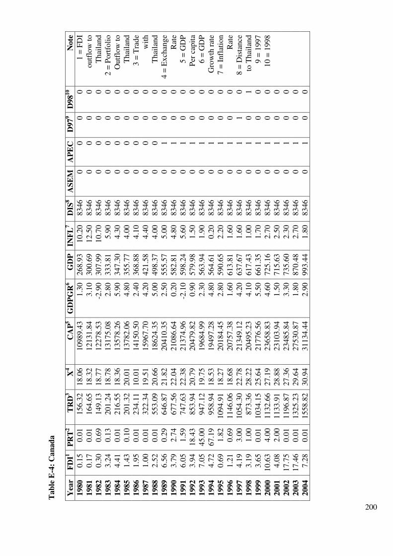
200
Tab
le E
-4:
Can
ad
a
Yea
r F
DI1
P
RT
2
TR
D3
X4
CA
P5
GD
PG
R6
GD
P
INF
L7
DIS
8
AS
EM
A
PE
C
D97
9
D98
10
Note
1980
0.1
5
0.0
1
156.3
2
18.0
6
10989.4
3
1.3
0
268.9
3
10.2
0
8346
0
0
0
0
1 =
FD
I
1981
0.1
7
0.0
1
164.6
5
18.3
2
12131.8
4
3.1
0
300.6
9
12.5
0
8346
0
0
0
0
outf
low
to
1982
0.3
0
0.6
9
149.1
3
18.7
7
12278.5
3
-2.9
0
307.9
9
10.7
0
8346
0
0
0
0
Thai
land
1983
3.2
4
0.1
3
201.2
4
18.7
8
13175.0
8
2.8
0
333.8
1
5.9
0
8346
0
0
0
0
2 =
Port
foli
o
1984
4.4
1
0.0
1
216.5
5
18.3
6
13578.2
6
5.9
0
347.3
0
4.3
0
8346
0
0
0
0
Outf
low
to
1985
1.4
3
0.1
0
201.3
2
20.0
1
13782.0
6
4.8
0
355.7
7
4.0
0
8346
0
0
0
0
Thai
land
1986
1.9
5
0.0
1
234.1
1
10.0
1
14150.5
0
2.4
0
368.8
8
4.1
0
8346
0
0
0
0
3 =
Tra
de
1987
1.0
0
0.0
1
322.3
4
19.5
1
15967.7
0
4.2
0
421.5
8
4.4
0
8346
0
0
0
0
wit
h
1988
2.5
2
0.0
1
553.0
9
20.6
6
18624.3
5
5.0
0
498.3
7
4.0
0
8346
0
0
0
0
Thai
land
1989
6.5
6
0.2
9
646.8
7
21.8
2
20410.3
5
2.5
0
555.5
7
5.0
0
8346
0
1
0
0
4 =
Ex
chan
ge
1990
3.7
9
2.7
4
677.5
6
22.0
4
21086.6
4
0.2
0
582.8
1
4.8
0
8346
0
1
0
0
Rat
e
1991
6.0
5
1.5
9
747.6
3
22.3
8
21374.9
6
-2.1
0
598.2
4
5.6
0
8346
0
1
0
0
5 =
GD
P
1992
3.9
4
18.4
3
853.9
4
20.7
9
20479.8
2
0.9
0
579.9
8
1.5
0
8346
0
1
0
0
Per
cap
ita
1993
7.0
5
45.0
0
947.1
2
19.7
5
19684.9
9
2.3
0
563.9
4
1.9
0
8346
0
1
0
0
6 =
GD
P
1994
4.7
2
67.1
9
958.9
4
18.5
3
19497.2
8
4.8
0
564.6
1
0.2
0
8346
0
1
0
0
Gro
wth
rat
e
1995
0.6
9
1.8
2
1094.9
1
18.2
7
20184.4
5
2.8
0
590.6
5
2.2
0
8346
0
1
0
0
7 =
Infl
atio
n
1996
1.2
1
0.6
9
1146.0
6
18.6
8
20757.3
8
1.6
0
613.8
1
1.6
0
8346
0
1
0
0
Rat
e
1997
4.1
9
3.0
0
1054.3
0
22.7
8
21349.1
2
4.2
0
637.6
7
1.6
0
8346
0
1
1
0
8 =
Dis
tance
1998
3.1
9
1.0
0
873.3
6
28.2
2
20495.2
3
4.1
0
617.4
3
1.0
0
8346
0
1
0
1
to T
hai
land
1999
3.6
5
0.0
1
1034.1
5
25.6
4
21776.5
6
5.5
0
661.3
5
1.7
0
8346
0
1
0
0
9 =
1997
2000
10.6
3
4.0
0
1132.6
6
27.1
9
23658.8
3
4.6
0
725.1
6
2.7
0
8346
0
1
0
0
10 =
1998
2001
4.0
8
2.0
0
1133.9
1
28.8
8
23103.9
4
1.5
0
715.6
3
2.5
0
8346
0
1
0
0
2002
17.7
5
0.0
1
1196.8
7
27.3
6
23485.8
4
3.3
0
735.6
0
2.3
0
8346
0
1
0
0
2003
17.4
6
0.0
1
1325.2
3
29.6
4
27530.8
7
1.8
0
870.4
8
2.7
0
8346
0
1
0
0
2004
7.2
8
0.0
1
1558.8
2
30.9
4
31134.4
4
2.9
0
993.4
4
1.8
0
8346
0
1
0
0
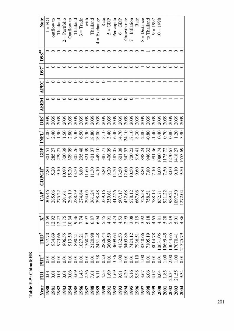
201
Tab
le E
-5:
Ch
ina&
HK
Y
ear
FD
I1
PR
T2
TR
D3
X4
CA
P5
GD
PG
R6
GD
P
INF
L7
DIS
8
AS
EM
A
PE
C
D97
9
D98
10
Note
1980
0.0
1
0.0
1
957.7
0
12.6
9
305.4
6
7.8
0
301.5
1
6.0
0
2039
0
0
0
0
1 =
FD
I
1981
0.0
1
0.0
1
934.6
9
12.9
2
285.0
6
5.2
0
285.2
7
2.4
0
2039
0
0
0
0
outf
low
to
1982
0.0
1
0.0
1
973.6
6
12.2
7
275.2
2
9.1
0
279.7
7
1.9
0
2039
0
0
0
0
Thai
land
1983
0.0
1
0.0
1
806.5
5
11.7
5
291.6
1
10.9
0
300.3
8
1.5
0
2039
0
0
0
0
2 =
Port
foli
o
1984
0.0
6
0.0
1
913.5
9
10.3
4
296.1
9
15.2
0
309.0
9
2.8
0
2039
0
0
0
0
Outf
low
to
1985
3.6
9
0.0
1
890.2
1
9.3
6
288.3
9
13.5
0
305.2
6
9.3
0
2039
0
0
0
0
Thai
land
1986
1.4
3
0.0
1
1027.2
1
7.7
4
274.8
4
8.8
0
295.4
8
6.5
0
2039
0
0
0
0
3 =
Tra
de
1987
2.5
6
0.0
1
1568.2
9
6.9
7
294.0
5
11.6
0
321.3
9
7.3
0
2039
0
0
0
0
wit
h
1988
7.6
1
0.0
1
2120.9
8
6.8
7
361.2
4
11.3
0
401.0
7
18.8
0
2039
0
0
0
0
Thai
land
1989
6.1
1
0.3
8
2431.4
8
6.9
4
398.4
8
4.1
0
449.1
0
18.0
0
2039
0
0
0
0
4 =
Ex
chan
ge
1990
4.5
3
0.2
3
2826.4
4
5.4
5
339.1
6
3.8
0
387.7
7
3.1
0
2039
0
0
0
0
Rat
e
1991
1.6
9
0.0
1
3609.5
9
4.9
1
350.6
1
9.2
0
406.0
9
3.4
0
2039
0
1
0
0
5 =
GD
P
1992
1.6
9
3.3
6
3609.6
4
4.7
4
412.2
6
14.2
0
483.0
5
6.4
0
2039
0
1
0
0
Per
cap
ita
1993
9.9
1
1.0
0
4132.5
3
4.5
3
507.1
7
13.5
0
601.0
8
14.7
0
2039
0
1
0
0
6 =
GD
P
1994
4.2
9
0.0
1
5403.8
6
2.9
5
452.6
8
12.6
0
542.5
3
24.1
0
2039
0
1
0
0
Gro
wth
rat
e
1995
5.1
6
0.0
1
7424.1
2
3.0
8
578.1
2
10.5
0
700.2
2
17.1
0
2039
0
1
0
0
7 =
Infl
atio
n
1996
5.9
8
0.1
0
7936.5
1
3.1
9
667.0
6
9.6
0
816.4
1
8.3
0
2039
1
1
0
0
Rat
e
1997
3.6
7
1.0
0
8348.6
6
3.9
2
726.5
8
8.8
0
898.2
4
2.8
0
2039
1
1
1
0
8 =
Dis
tance
1998
6.0
6
0.0
1
7105.1
9
5.1
8
758.5
1
7.8
0
946.3
2
-0.8
0
2039
1
1
0
1
to T
hai
land
1999
4.0
7
0.0
1
8014.7
8
4.6
5
788.1
3
7.1
0
991.3
6
-1.4
0
2039
1
1
0
0
9 =
1997
2000
8.0
4
0.0
1
10631.0
5
4.8
1
852.7
1
8.0
0
1080.7
4
0.4
0
2039
1
1
0
0
10 =
1998
2001
1.8
5
1.0
0
10699.4
5
5.2
8
921.2
2
7.5
0
1175.7
2
0.7
0
2039
1
1
0
0
2002
20.3
4
2.0
0
13044.6
5
5.1
9
989.2
1
8.0
0
1270.6
7
-0.8
0
2039
1
1
0
0
2003
21.5
5
1.0
0
17070.4
1
5.0
1
1097.5
0
9.1
0
1418.2
7
1.2
0
2039
1
1
0
0
2004
9.3
4
0.0
1
21525.7
9
4.8
6
1272.0
4
9.5
0
1653.6
9
3.9
0
2039
1
1
0
0
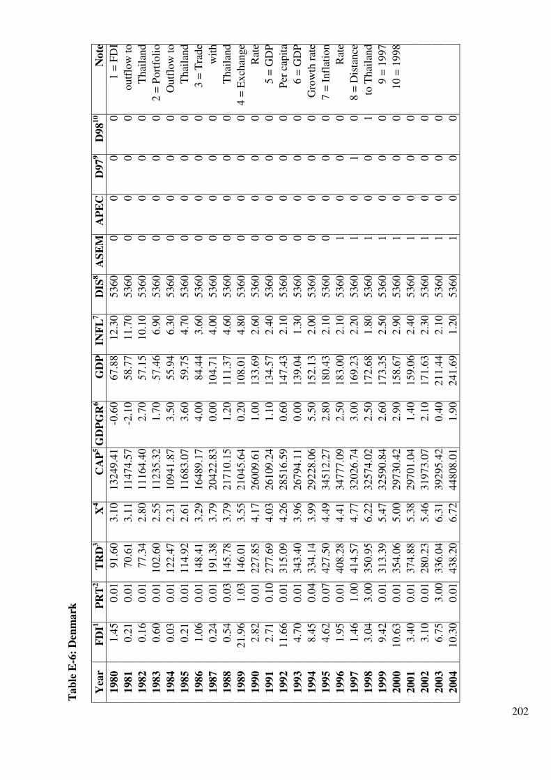
202
Tab
le E
-6:
Den
ma
rk
Yea
r F
DI1
P
RT
2
TR
D3
X4
CA
P5 G
DP
GR
6
GD
P
INF
L7
DIS
8
AS
EM
A
PE
C
D97
9
D98
10
Note
1980
1.4
5
0.0
1
91.6
0
3.1
0
13249.4
1
-0.6
0
67.8
8
12.3
0
5360
0
0
0
0
1 =
FD
I
1981
0.2
1
0.0
1
70.6
1
3.1
1
11474.5
7
-2.1
0
58.7
7
11.7
0
5360
0
0
0
0
outf
low
to
1982
0.1
6
0.0
1
77.3
4
2.8
0
11164.4
0
2.7
0
57.1
5
10.1
0
5360
0
0
0
0
Thai
land
1983
0.6
0
0.0
1
102.6
0
2.5
5
11235.3
2
1.7
0
57.4
6
6.9
0
5360
0
0
0
0
2 =
Port
foli
o
1984
0.0
3
0.0
1
122.4
7
2.3
1
10941.8
7
3.5
0
55.9
4
6.3
0
5360
0
0
0
0
Outf
low
to
1985
0.2
1
0.0
1
114.9
2
2.6
1
11683.0
7
3.6
0
59.7
5
4.7
0
5360
0
0
0
0
Thai
land
1986
1.0
6
0.0
1
148.4
1
3.2
9
16489.1
7
4.0
0
84.4
4
3.6
0
5360
0
0
0
0
3 =
Tra
de
1987
0.2
4
0.0
1
191.3
8
3.7
9
20422.8
3
0.0
0
104.7
1
4.0
0
5360
0
0
0
0
wit
h
1988
0.5
4
0.0
3
145.7
8
3.7
9
21710.1
5
1.2
0
111.3
7
4.6
0
5360
0
0
0
0
Thai
land
1989
21.9
6
1.0
3
146.0
1
3.5
5
21045.6
4
0.2
0
108.0
1
4.8
0
5360
0
0
0
0
4 =
Ex
chan
ge
1990
2.8
2
0.0
1
227.8
5
4.1
7
26009.6
1
1.0
0
133.6
9
2.6
0
5360
0
0
0
0
Rat
e
1991
2.7
1
0.1
0
277.6
9
4.0
3
26109.2
4
1.1
0
134.5
7
2.4
0
5360
0
0
0
0
5 =
GD
P
1992
11.6
6
0.0
1
315.0
9
4.2
6
28516.5
9
0.6
0
147.4
3
2.1
0
5360
0
0
0
0
Per
cap
ita
1993
4.7
0
0.0
1
343.4
0
3.9
6
26794.1
1
0.0
0
139.0
4
1.3
0
5360
0
0
0
0
6 =
GD
P
1994
8.4
5
0.0
4
334.1
4
3.9
9
29228.0
6
5.5
0
152.1
3
2.0
0
5360
0
0
0
0
Gro
wth
rat
e
1995
4.6
2
0.0
7
427.5
0
4.4
9
34512.2
7
2.8
0
180.4
3
2.1
0
5360
0
0
0
0
7 =
Infl
atio
n
1996
1.9
5
0.0
1
408.2
8
4.4
1
34777.0
9
2.5
0
183.0
0
2.1
0
5360
1
0
0
0
Rat
e
1997
1.4
6
1.0
0
414.5
7
4.7
7
32026.7
4
3.0
0
169.2
3
2.2
0
5360
1
0
1
0
8 =
Dis
tance
1998
3.0
4
3.0
0
350.9
5
6.2
2
32574.0
2
2.5
0
172.6
8
1.8
0
5360
1
0
0
1
to T
hai
land
1999
9.4
2
0.0
1
313.3
9
5.4
7
32590.8
4
2.6
0
173.3
5
2.5
0
5360
1
0
0
0
9 =
1997
2000
10.6
3
0.0
1
354.0
6
5.0
0
29730.4
2
2.9
0
158.6
7
2.9
0
5360
1
0
0
0
10 =
1998
2001
3.4
0
0.0
1
374.8
8
5.3
8
29701.0
4
1.4
0
159.0
6
2.4
0
5360
1
0
0
0
2002
3.1
0
0.0
1
280.2
3
5.4
6
31973.0
7
2.1
0
171.6
3
2.3
0
5360
1
0
0
0
2003
6.7
5
3.0
0
336.0
4
6.3
1
39295.4
2
0.4
0
211.4
4
2.1
0
5360
1
0
0
0
2004
10.3
0
0.0
1
438.2
0
6.7
2
44808.0
1
1.9
0
241.6
9
1.2
0
5360
1
0
0
0
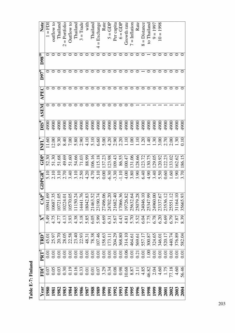
203
Tab
le E
-7:
Fin
lan
d
Yea
r F
DI1
P
RT
2
TR
D3
X4
CA
P5
GD
PG
R6
GD
P
INF
L7
DIS
8
AS
EM
A
PE
C
D97
9
D98
10
Note
1980
0.0
7
0.0
1
45.0
1
5.4
9
10941.6
9
5.1
0
52.3
0
11.6
0
4900
0
0
0
0
1 =
FD
I
1981
0.0
5
0.0
1
25.9
7
4.7
5
10687.3
5
2.1
0
51.3
0
12.0
0
4900
0
0
0
0
outf
low
to
1982
0.0
3
0.0
1
20.7
0
4.7
7
10721.0
5
3.1
0
51.6
8
9.3
0
4900
0
0
0
0
Thai
land
1983
0.3
0
0.0
1
28.0
5
4.1
3
10224.0
1
2.7
0
49.6
9
8.4
0
4900
0
0
0
0
2 =
Port
foli
o
1984
0.1
9
0.0
1
22.5
8
3.9
3
10570.0
5
3.4
0
51.6
0
7.0
0
4900
0
0
0
0
Outf
low
to
1985
0.1
6
0.0
1
23.4
0
4.3
8
11150.2
4
3.1
0
54.6
6
5.8
0
4900
0
0
0
0
Thai
land
1986
0.3
3
0.0
1
22.9
3
5.1
8
14441.7
6
2.5
0
71.0
3
2.9
0
4900
0
0
0
0
3 =
Tra
de
1987
0.0
1
0.0
1
48.3
1
5.8
5
18042.8
3
4.2
0
88.9
9
4.1
0
4900
0
0
0
0
wit
h
1988
0.0
1
0.0
1
78.3
8
6.0
5
21463.5
2
4.7
0
106.1
6
5.1
0
4900
0
0
0
0
Thai
land
1989
0.0
7
0.0
1
107.4
6
5.9
9
23190.7
4
5.1
0
115.1
8
6.6
0
4900
0
0
0
0
4 =
Ex
chan
ge
1990
3.2
9
0.0
1
158.6
3
6.6
9
27496.0
6
0.0
0
137.2
3
5.0
0
4900
0
0
0
0
Rat
e
1991
0.3
4
0.0
1
173.1
1
6.3
1
24702.2
0
-6.3
0
123.9
8
4.2
0
4900
0
0
0
0
5 =
GD
P
1992
0.0
8
0.0
1
204.2
9
5.6
7
21682.4
0
-3.3
0
109.4
3
2.9
0
4900
0
0
0
0
Per
cap
ita
1993
0.9
8
0.0
1
368.8
0
4.4
3
17066.3
6
-1.1
0
86.5
5
2.2
0
4900
0
0
0
0
6 =
GD
P
1994
10.6
8
0.0
6
314.1
0
4.8
1
19726.8
2
4.0
0
100.4
7
1.1
0
4900
0
0
0
0
Gro
wth
rat
e
1995
8.8
7
0.0
1
464.6
1
5.7
0
25632.6
4
3.8
0
131.0
6
1.0
0
4900
0
0
0
0
7 =
Infl
atio
n
1996
2.1
1
0.2
1
569.6
1
5.5
2
25079.2
8
3.9
0
128.6
6
1.1
0
4900
1
0
0
0
Rat
e
1997
4.8
5
0.0
1
557.1
7
6.0
4
24046.1
0
6.4
0
123.7
2
1.2
0
4900
1
0
1
0
8 =
Dis
tance
1998
46.8
2
1.0
0
300.8
7
7.7
5
25347.9
9
4.9
0
130.7
5
1.4
0
4900
1
0
0
1
to T
hai
land
1999
2.0
4
0.0
1
324.6
5
6.7
8
24960.0
0
3.4
0
129.0
5
1.3
0
4900
1
0
0
0
9 =
1997
2000
4.6
0
0.0
1
346.0
1
6.2
0
23337.6
7
5.5
0
120.9
2
3.0
0
4900
1
0
0
0
10 =
1998
2001
1.7
5
0.0
1
520.1
7
6.6
9
23536.1
2
0.6
0
122.2
3
2.7
0
4900
1
0
0
0
2002
77.1
8
0.0
1
440.7
4
6.7
9
25551.1
2
1.6
0
133.0
2
2.0
0
4900
1
0
0
0
2003
4.6
0
0.0
1
376.8
9
7.8
7
31164.1
0
1.9
0
162.6
2
1.3
0
4900
1
0
0
0
2004
56.4
6
0.0
1
582.0
4
8.3
9
35665.9
3
3.7
0
186.1
5
0.1
0
4900
1
0
0
0
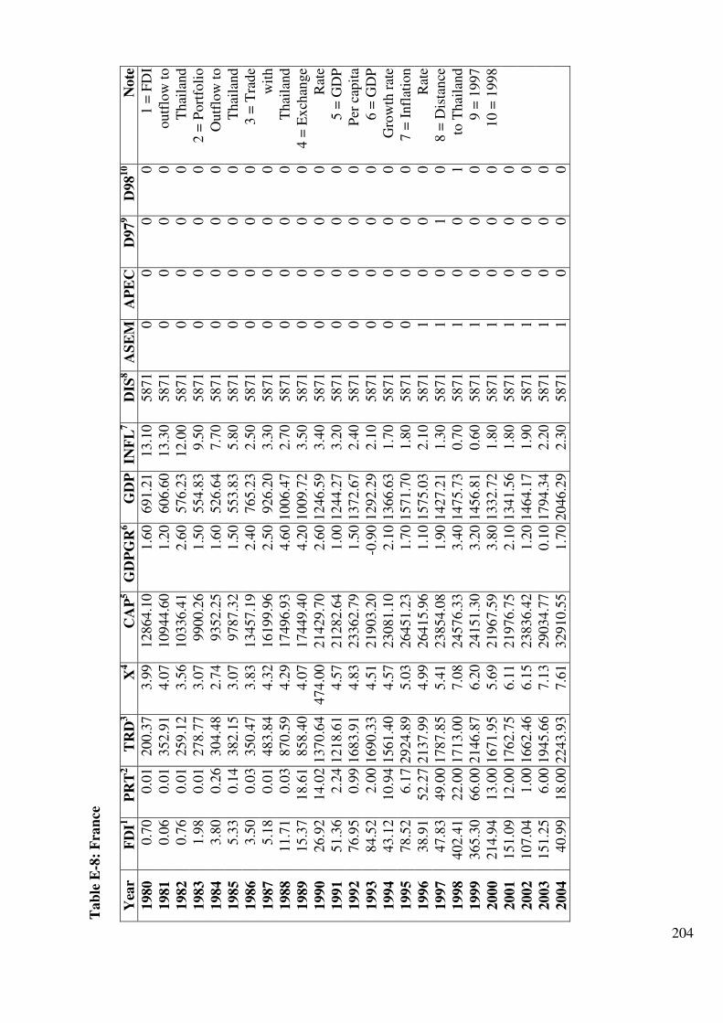
204
Tab
le E
-8:
Fra
nce
Yea
r F
DI1
P
RT
2
TR
D3
X4
CA
P5
GD
PG
R6
GD
P
INF
L7
DIS
8
AS
EM
A
PE
C
D97
9
D98
10
Note
1980
0.7
0
0.0
1
200.3
7
3.9
9
12864.1
0
1.6
0
691.2
1
13.1
0
5871
0
0
0
0
1 =
FD
I
1981
0.0
6
0.0
1
352.9
1
4.0
7
10944.6
0
1.2
0
606.6
0
13.3
0
5871
0
0
0
0
outf
low
to
1982
0.7
6
0.0
1
259.1
2
3.5
6
10336.4
1
2.6
0
576.2
3
12.0
0
5871
0
0
0
0
Thai
land
1983
1.9
8
0.0
1
278.7
7
3.0
7
9900.2
6
1.5
0
554.8
3
9.5
0
5871
0
0
0
0
2 =
Port
foli
o
1984
3.8
0
0.2
6
304.4
8
2.7
4
9352.2
5
1.6
0
526.6
4
7.7
0
5871
0
0
0
0
Outf
low
to
1985
5.3
3
0.1
4
382.1
5
3.0
7
9787.3
2
1.5
0
553.8
3
5.8
0
5871
0
0
0
0
Thai
land
1986
3.5
0
0.0
3
350.4
7
3.8
3
13457.1
9
2.4
0
765.2
3
2.5
0
5871
0
0
0
0
3 =
Tra
de
1987
5.1
8
0.0
1
483.8
4
4.3
2
16199.9
6
2.5
0
926.2
0
3.3
0
5871
0
0
0
0
wit
h
1988
11.7
1
0.0
3
870.5
9
4.2
9
17496.9
3
4.6
0 1
006.4
7
2.7
0
5871
0
0
0
0
Thai
land
1989
15.3
7
18.6
1
858.4
0
4.0
7
17449.4
0
4.2
0 1
009.7
2
3.5
0
5871
0
0
0
0
4 =
Ex
chan
ge
1990
26.9
2
14.0
2 1
370.6
4
474.0
0
21429.7
0
2.6
0 1
246.5
9
3.4
0
5871
0
0
0
0
Rat
e
1991
51.3
6
2.2
4 1
218.6
1
4.5
7
21282.6
4
1.0
0 1
244.2
7
3.2
0
5871
0
0
0
0
5 =
GD
P
1992
76.9
5
0.9
9 1
683.9
1
4.8
3
23362.7
9
1.5
0 1
372.6
7
2.4
0
5871
0
0
0
0
Per
cap
ita
1993
84.5
2
2.0
0 1
690.3
3
4.5
1
21903.2
0
-0.9
0 1
292.2
9
2.1
0
5871
0
0
0
0
6 =
GD
P
1994
43.1
2
10.9
4 1
561.4
0
4.5
7
23081.1
0
2.1
0 1
366.6
3
1.7
0
5871
0
0
0
0
Gro
wth
rat
e
1995
78.5
2
6.1
7 2
924.8
9
5.0
3
26451.2
3
1.7
0 1
571.7
0
1.8
0
5871
0
0
0
0
7 =
Infl
atio
n
1996
38.9
1
52.2
7 2
137.9
9
4.9
9
26415.9
6
1.1
0 1
575.0
3
2.1
0
5871
1
0
0
0
Rat
e
1997
47.8
3
49.0
0 1
787.8
5
5.4
1
23854.0
8
1.9
0 1
427.2
1
1.3
0
5871
1
0
1
0
8 =
Dis
tance
1998
402.4
1
22.0
0 1
713.0
0
7.0
8
24576.3
3
3.4
0 1
475.7
3
0.7
0
5871
1
0
0
1
to T
hai
land
1999
365.3
0
66.0
0 2
146.8
7
6.2
0
24151.3
0
3.2
0 1
456.8
1
0.6
0
5871
1
0
0
0
9 =
1997
2000
214.9
4
13.0
0 1
671.9
5
5.6
9
21967.5
9
3.8
0 1
332.7
2
1.8
0
5871
1
0
0
0
10 =
1998
2001
151.0
9
12.0
0 1
762.7
5
6.1
1
21976.7
5
2.1
0 1
341.5
6
1.8
0
5871
1
0
0
0
2002
107.0
4
1.0
0 1
662.4
6
6.1
5
23836.4
2
1.2
0 1
464.1
7
1.9
0
5871
1
0
0
0
2003
151.2
5
6.0
0 1
945.6
6
7.1
3
29034.7
7
0.1
0 1
794.3
4
2.2
0
5871
1
0
0
0
2004
40.9
9
18.0
0 2
243.9
3
7.6
1
32910.5
5
1.7
0 2
046.2
9
2.3
0
5871
1
0
0
0
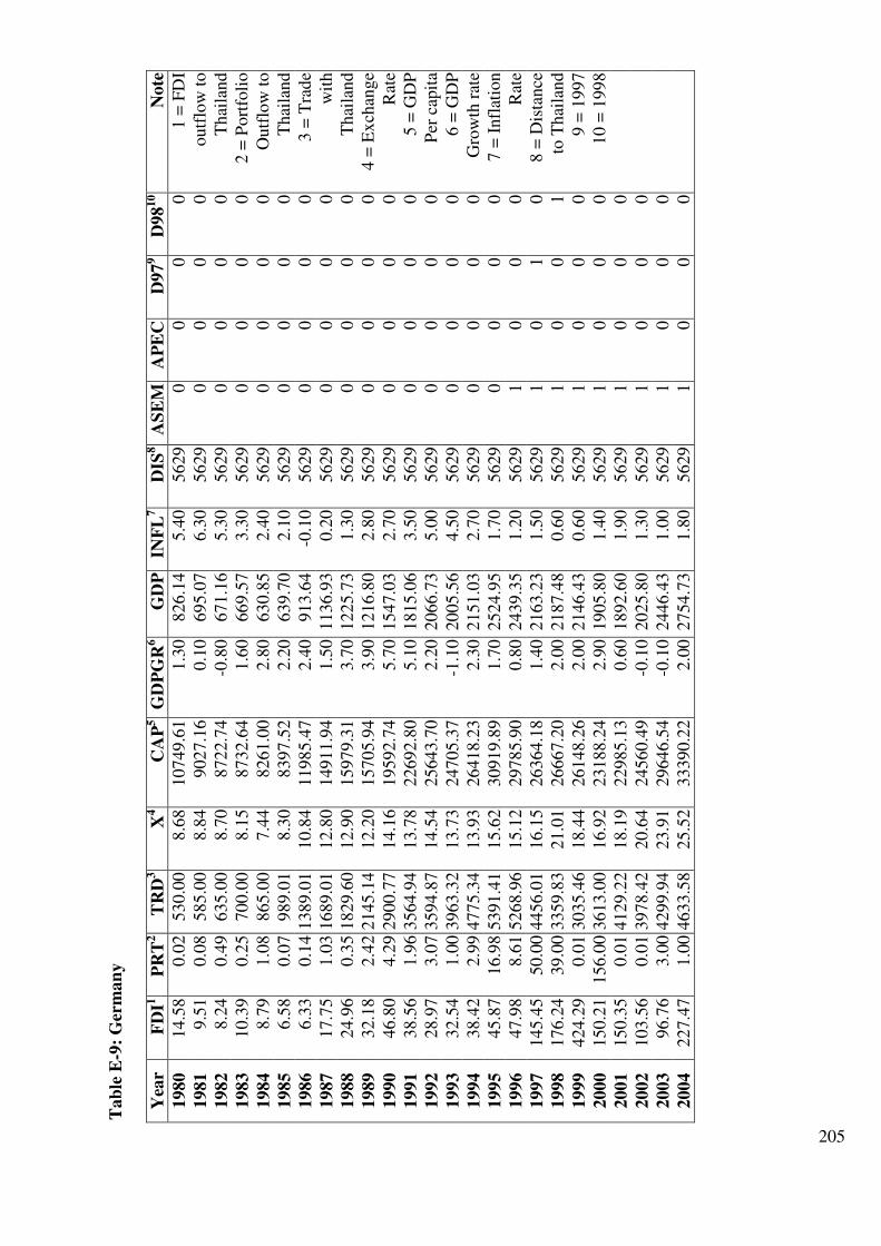
205
Tab
le E
-9:
Ger
man
y
Yea
r F
DI1
P
RT
2
TR
D3
X4
CA
P5
GD
PG
R6
GD
P
INF
L7
DIS
8
AS
EM
A
PE
C
D97
9
D98
10
Note
1980
14.5
8
0.0
2
530.0
0
8.6
8
10749.6
1
1.3
0
826.1
4
5.4
0
5629
0
0
0
0
1 =
FD
I
1981
9.5
1
0.0
8
585.0
0
8.8
4
9027.1
6
0.1
0
695.0
7
6.3
0
5629
0
0
0
0
outf
low
to
1982
8.2
4
0.4
9
635.0
0
8.7
0
8722.7
4
-0.8
0
671.1
6
5.3
0
5629
0
0
0
0
Thai
land
1983
10.3
9
0.2
5
700.0
0
8.1
5
8732.6
4
1.6
0
669.5
7
3.3
0
5629
0
0
0
0
2 =
Port
foli
o
1984
8.7
9
1.0
8
865.0
0
7.4
4
8261.0
0
2.8
0
630.8
5
2.4
0
5629
0
0
0
0
Outf
low
to
1985
6.5
8
0.0
7
989.0
1
8.3
0
8397.5
2
2.2
0
639.7
0
2.1
0
5629
0
0
0
0
Thai
land
1986
6.3
3
0.1
4 1
389.0
1
10.8
4
11985.4
7
2.4
0
913.6
4
-0.1
0
5629
0
0
0
0
3 =
Tra
de
1987
17.7
5
1.0
3 1
689.0
1
12.8
0
14911.9
4
1.5
0 1136.9
3
0.2
0
5629
0
0
0
0
wit
h
1988
24.9
6
0.3
5 1
829.6
0
12.9
0
15979.3
1
3.7
0 1225.7
3
1.3
0
5629
0
0
0
0
Thai
land
1989
32.1
8
2.4
2 2
145.1
4
12.2
0
15705.9
4
3.9
0 1216.8
0
2.8
0
5629
0
0
0
0
4 =
Ex
chan
ge
1990
46.8
0
4.2
9 2
900.7
7
14.1
6
19592.7
4
5.7
0 1547.0
3
2.7
0
5629
0
0
0
0
Rat
e
1991
38.5
6
1.9
6 3
564.9
4
13.7
8
22692.8
0
5.1
0 1815.0
6
3.5
0
5629
0
0
0
0
5 =
GD
P
1992
28.9
7
3.0
7 3
594.8
7
14.5
4
25643.7
0
2.2
0 2066.7
3
5.0
0
5629
0
0
0
0
Per
cap
ita
1993
32.5
4
1.0
0 3
963.3
2
13.7
3
24705.3
7
-1.1
0 2005.5
6
4.5
0
5629
0
0
0
0
6 =
GD
P
1994
38.4
2
2.9
9 4
775.3
4
13.9
3
26418.2
3
2.3
0 2151.0
3
2.7
0
5629
0
0
0
0
Gro
wth
rat
e
1995
45.8
7
16.9
8 5
391.4
1
15.6
2
30919.8
9
1.7
0 2524.9
5
1.7
0
5629
0
0
0
0
7 =
Infl
atio
n
1996
47.9
8
8.6
1 5
268.9
6
15.1
2
29785.9
0
0.8
0 2439.3
5
1.2
0
5629
1
0
0
0
Rat
e
1997
145.4
5
50.0
0 4
456.0
1
16.1
5
26364.1
8
1.4
0 2163.2
3
1.5
0
5629
1
0
1
0
8 =
Dis
tance
1998
176.2
4
39.0
0 3
359.8
3
21.0
1
26667.2
0
2.0
0 2187.4
8
0.6
0
5629
1
0
0
1
to T
hai
land
1999
424.2
9
0.0
1 3
035.4
6
18.4
4
26148.2
6
2.0
0 2146.4
3
0.6
0
5629
1
0
0
0
9 =
1997
2000
150.2
1
156.0
0 3
613.0
0
16.9
2
23188.2
4
2.9
0 1905.8
0
1.4
0
5629
1
0
0
0
10 =
1998
2001
150.3
5
0.0
1 4
129.2
2
18.1
9
22985.1
3
0.6
0 1892.6
0
1.9
0
5629
1
0
0
0
2002
103.5
6
0.0
1 3
978.4
2
20.6
4
24560.4
9
-0.1
0 2025.8
0
1.3
0
5629
1
0
0
0
2003
96.7
6
3.0
0 4
299.9
4
23.9
1
29646.5
4
-0.1
0 2446.4
3
1.0
0
5629
1
0
0
0
2004
227.4
7
1.0
0 4
633.5
8
25.5
2
33390.2
2
2.0
0 2754.7
3
1.8
0
5629
1
0
0
0
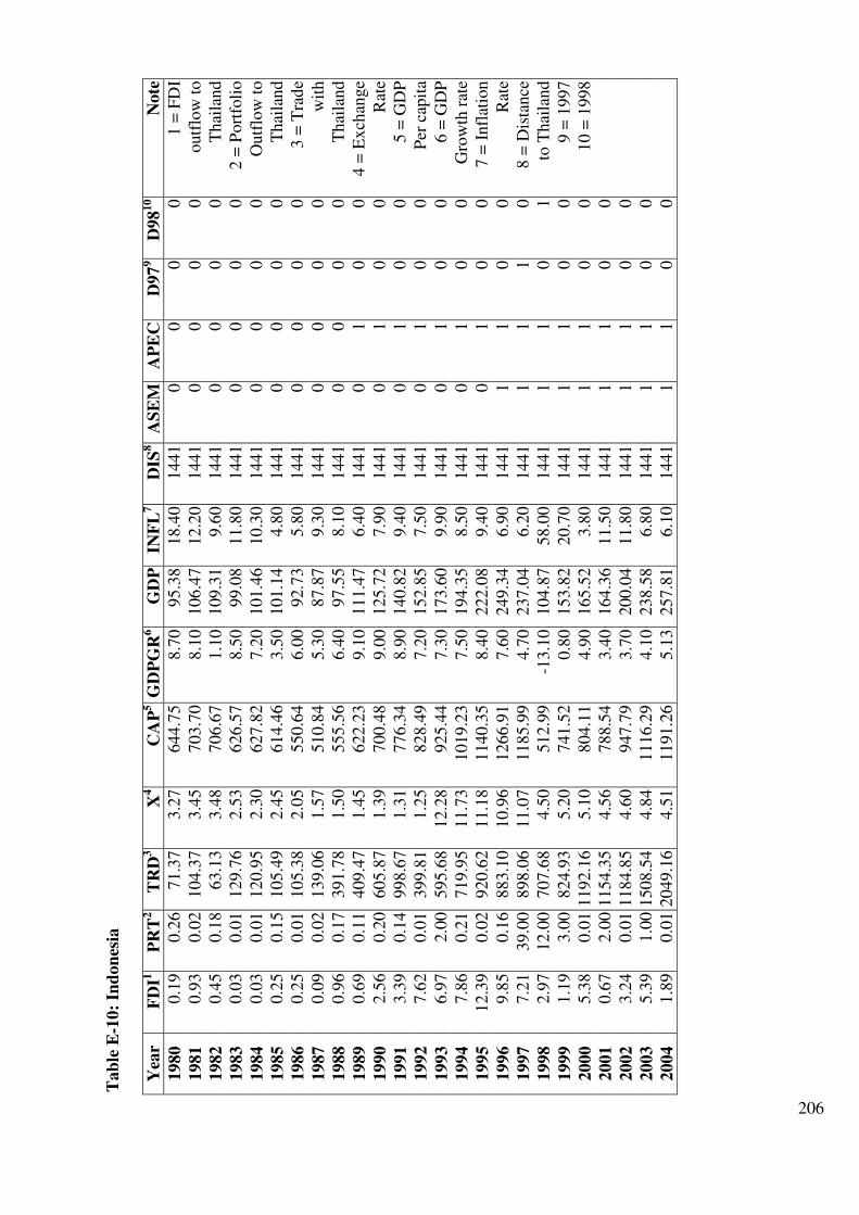
206
Tab
le E
-10:
Ind
on
esia
Yea
r F
DI1
P
RT
2
TR
D3
X4
CA
P5 G
DP
GR
6
GD
P
INF
L7
DIS
8
AS
EM
A
PE
C
D97
9
D98
10
Note
1980
0.1
9
0.2
6
71.3
7
3.2
7
644.7
5
8.7
0
95.3
8
18.4
0
1441
0
0
0
0
1 =
FD
I
1981
0.9
3
0.0
2
104.3
7
3.4
5
703.7
0
8.1
0
106.4
7
12.2
0
1441
0
0
0
0
outf
low
to
1982
0.4
5
0.1
8
63.1
3
3.4
8
706.6
7
1.1
0
109.3
1
9.6
0
1441
0
0
0
0
Thai
land
1983
0.0
3
0.0
1
129.7
6
2.5
3
626.5
7
8.5
0
99.0
8
11.8
0
1441
0
0
0
0
2 =
Port
foli
o
1984
0.0
3
0.0
1
120.9
5
2.3
0
627.8
2
7.2
0
101.4
6
10.3
0
1441
0
0
0
0
Outf
low
to
1985
0.2
5
0.1
5
105.4
9
2.4
5
614.4
6
3.5
0
101.1
4
4.8
0
1441
0
0
0
0
Thai
land
1986
0.2
5
0.0
1
105.3
8
2.0
5
550.6
4
6.0
0
92.7
3
5.8
0
1441
0
0
0
0
3 =
Tra
de
1987
0.0
9
0.0
2
139.0
6
1.5
7
510.8
4
5.3
0
87.8
7
9.3
0
1441
0
0
0
0
wit
h
1988
0.9
6
0.1
7
391.7
8
1.5
0
555.5
6
6.4
0
97.5
5
8.1
0
1441
0
0
0
0
Thai
land
1989
0.6
9
0.1
1
409.4
7
1.4
5
622.2
3
9.1
0
111.4
7
6.4
0
1441
0
1
0
0
4 =
Ex
chan
ge
1990
2.5
6
0.2
0
605.8
7
1.3
9
700.4
8
9.0
0
125.7
2
7.9
0
1441
0
1
0
0
Rat
e
1991
3.3
9
0.1
4
998.6
7
1.3
1
776.3
4
8.9
0
140.8
2
9.4
0
1441
0
1
0
0
5 =
GD
P
1992
7.6
2
0.0
1
399.8
1
1.2
5
828.4
9
7.2
0
152.8
5
7.5
0
1441
0
1
0
0
Per
cap
ita
1993
6.9
7
2.0
0
595.6
8
12.2
8
925.4
4
7.3
0
173.6
0
9.9
0
1441
0
1
0
0
6 =
GD
P
1994
7.8
6
0.2
1
719.9
5
11.7
3
1019.2
3
7.5
0
194.3
5
8.5
0
1441
0
1
0
0
Gro
wth
rat
e
1995
12.3
9
0.0
2
920.6
2
11.1
8
1140.3
5
8.4
0
222.0
8
9.4
0
1441
0
1
0
0
7 =
Infl
atio
n
1996
9.8
5
0.1
6
883.1
0
10.9
6
1266.9
1
7.6
0
249.3
4
6.9
0
1441
1
1
0
0
Rat
e
1997
7.2
1
39.0
0
898.0
6
11.0
7
1185.9
9
4.7
0
237.0
4
6.2
0
1441
1
1
1
0
8 =
Dis
tance
1998
2.9
7
12.0
0
707.6
8
4.5
0
512.9
9
-13.1
0
104.8
7
58.0
0
1441
1
1
0
1
to T
hai
land
1999
1.1
9
3.0
0
824.9
3
5.2
0
741.5
2
0.8
0
153.8
2
20.7
0
1441
1
1
0
0
9 =
1997
2000
5.3
8
0.0
1 1
192.1
6
5.1
0
804.1
1
4.9
0
165.5
2
3.8
0
1441
1
1
0
0
10 =
1998
2001
0.6
7
2.0
0 1
154.3
5
4.5
6
788.5
4
3.4
0
164.3
6
11.5
0
1441
1
1
0
0
2002
3.2
4
0.0
1 1
184.8
5
4.6
0
947.7
9
3.7
0
200.0
4
11.8
0
1441
1
1
0
0
2003
5.3
9
1.0
0 1
508.5
4
4.8
4
1116.2
9
4.1
0
238.5
8
6.8
0
1441
1
1
0
0
2004
1.8
9
0.0
1 2
049.1
6
4.5
1
1191.2
6
5.1
3
257.8
1
6.1
0
1441
1
1
0
0
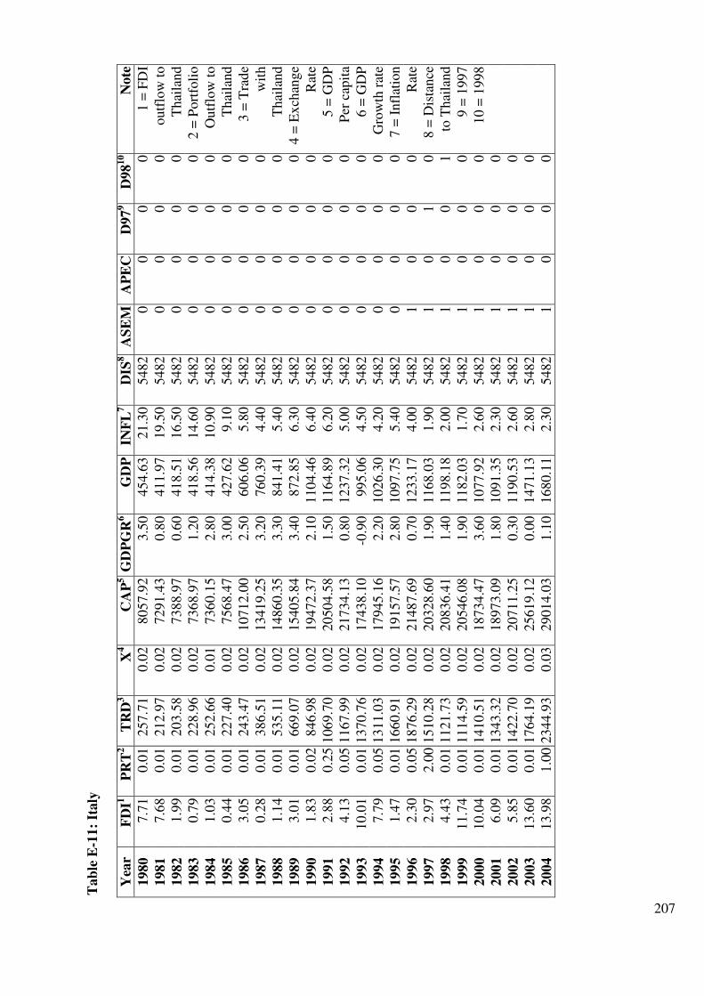
207
Tab
le E
-11:
Italy
Yea
r F
DI1
P
RT
2
TR
D3
X4
CA
P5 G
DP
GR
6
GD
P
INF
L7
DIS
8
AS
EM
A
PE
C
D97
9
D98
10
Note
1980
7.7
1
0.0
1
257.7
1
0.0
2
8057.9
2
3.5
0
454.6
3
21.3
0
5482
0
0
0
0
1 =
FD
I
1981
7.6
8
0.0
1
212.9
7
0.0
2
7291.4
3
0.8
0
411.9
7
19.5
0
5482
0
0
0
0
outf
low
to
1982
1.9
9
0.0
1
203.5
8
0.0
2
7388.9
7
0.6
0
418.5
1
16.5
0
5482
0
0
0
0
Thai
land
1983
0.7
9
0.0
1
228.9
6
0.0
2
7368.9
7
1.2
0
418.5
6
14.6
0
5482
0
0
0
0
2 =
Port
foli
o
1984
1.0
3
0.0
1
252.6
6
0.0
1
7360.1
5
2.8
0
414.3
8
10.9
0
5482
0
0
0
0
Outf
low
to
1985
0.4
4
0.0
1
227.4
0
0.0
2
7568.4
7
3.0
0
427.6
2
9.1
0
5482
0
0
0
0
Thai
land
1986
3.0
5
0.0
1
243.4
7
0.0
2
10712.0
0
2.5
0
606.0
6
5.8
0
5482
0
0
0
0
3 =
Tra
de
1987
0.2
8
0.0
1
386.5
1
0.0
2
13419.2
5
3.2
0
760.3
9
4.4
0
5482
0
0
0
0
wit
h
1988
1.1
4
0.0
1
535.1
1
0.0
2
14860.3
5
3.3
0
841.4
1
5.4
0
5482
0
0
0
0
Thai
land
1989
3.0
1
0.0
1
669.0
7
0.0
2
15405.8
4
3.4
0
872.8
5
6.3
0
5482
0
0
0
0
4 =
Ex
chan
ge
1990
1.8
3
0.0
2
846.9
8
0.0
2
19472.3
7
2.1
0
1104.4
6
6.4
0
5482
0
0
0
0
Rat
e
1991
2.8
8
0.2
5 1
069.7
0
0.0
2
20504.5
8
1.5
0
1164.8
9
6.2
0
5482
0
0
0
0
5 =
GD
P
1992
4.1
3
0.0
5 1
167.9
9
0.0
2
21734.1
3
0.8
0
1237.3
2
5.0
0
5482
0
0
0
0
Per
cap
ita
1993
10.0
1
0.0
1 1
370.7
6
0.0
2
17438.1
0
-0.9
0
995.0
6
4.5
0
5482
0
0
0
0
6 =
GD
P
1994
7.7
9
0.0
5 1
311.0
3
0.0
2
17945.1
6
2.2
0
1026.3
0
4.2
0
5482
0
0
0
0
Gro
wth
rat
e
1995
1.4
7
0.0
1 1
660.9
1
0.0
2
19157.5
7
2.8
0
1097.7
5
5.4
0
5482
0
0
0
0
7 =
Infl
atio
n
1996
2.3
0
0.0
5 1
876.2
9
0.0
2
21487.6
9
0.7
0
1233.1
7
4.0
0
5482
1
0
0
0
Rat
e
1997
2.9
7
2.0
0 1
510.2
8
0.0
2
20328.6
0
1.9
0
1168.0
3
1.9
0
5482
1
0
1
0
8 =
Dis
tance
1998
4.4
3
0.0
1 1
121.7
3
0.0
2
20836.4
1
1.4
0
1198.1
8
2.0
0
5482
1
0
0
1
to T
hai
land
1999
11.7
4
0.0
1 1
114.5
9
0.0
2
20546.0
8
1.9
0
1182.0
3
1.7
0
5482
1
0
0
0
9 =
1997
2000
10.0
4
0.0
1 1
410.5
1
0.0
2
18734.4
7
3.6
0
1077.9
2
2.6
0
5482
1
0
0
0
10 =
1998
2001
6.0
9
0.0
1 1
343.3
2
0.0
2
18973.0
9
1.8
0
1091.3
5
2.3
0
5482
1
0
0
0
2002
5.8
5
0.0
1 1
422.7
0
0.0
2
20711.2
5
0.3
0
1190.5
3
2.6
0
5482
1
0
0
0
2003
13.6
0
0.0
1 1
764.1
9
0.0
2
25619.1
2
0.0
0
1471.1
3
2.8
0
5482
1
0
0
0
2004
13.9
8
1.0
0 2
344.9
3
0.0
3
29014.0
3
1.1
0
1680.1
1
2.3
0
5482
1
0
0
0
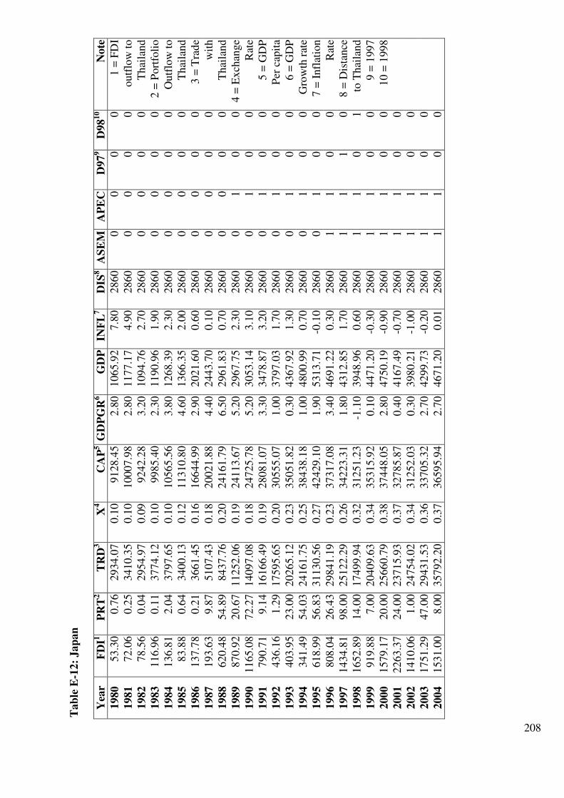
208
Tab
le E
-12:
Jap
an
Yea
r F
DI1
P
RT
2
TR
D3
X4
CA
P5 G
DP
GR
6
GD
P
INF
L7
DIS
8
AS
EM
A
PE
C
D97
9
D98
10
Note
1980
53.3
0
0.7
6
2934.0
7
0.1
0
9128.4
5
2.8
0
1065.9
2
7.8
0
2860
0
0
0
0
1 =
FD
I
1981
72.0
6
0.2
5
3410.3
5
0.1
0
10007.9
8
2.8
0
1177.1
7
4.9
0
2860
0
0
0
0
outf
low
to
1982
78.5
6
0.0
4
2954.9
7
0.0
9
9242.2
8
3.2
0
1094.7
6
2.7
0
2860
0
0
0
0
Thai
land
1983
116.9
6
0.1
1
3774.1
2
0.1
0
9985.4
0
2.3
0
1190.9
6
1.9
0
2860
0
0
0
0
2 =
Port
foli
o
1984
136.8
1
2.0
4
3797.6
5
0.1
0
10565.5
6
3.8
0
1268.3
9
2.3
0
2860
0
0
0
0
Outf
low
to
1985
83.8
8
0.6
4
3400.1
3
0.1
2
11310.8
0
4.6
0
1366.3
5
2.0
0
2860
0
0
0
0
Thai
land
1986
137.7
8
0.2
1
3661.4
5
0.1
6
16644.9
9
2.9
0
2021.6
0
0.6
0
2860
0
0
0
0
3 =
Tra
de
1987
193.6
3
9.8
7
5107.4
3
0.1
8
20021.8
8
4.4
0
2443.7
0
0.1
0
2860
0
0
0
0
wit
h
1988
620.4
8
54.8
9
8437.7
6
0.2
0
24161.7
9
6.5
0
2961.8
3
0.7
0
2860
0
0
0
0
Thai
land
1989
870.9
2
20.6
7
11252.0
6
0.1
9
24113.6
7
5.2
0
2967.7
5
2.3
0
2860
0
1
0
0
4 =
Ex
chan
ge
1990
1165.0
8
72.2
7
14097.0
8
0.1
8
24725.7
8
5.2
0
3053.1
4
3.1
0
2860
0
1
0
0
Rat
e
1991
790.7
1
9.1
4
16166.4
9
0.1
9
28081.0
7
3.3
0
3478.8
7
3.2
0
2860
0
1
0
0
5 =
GD
P
1992
436.1
6
1.2
9
17595.6
5
0.2
0
30555.0
7
1.0
0
3797.0
3
1.7
0
2860
0
1
0
0
Per
cap
ita
1993
403.9
5
23.0
0
20265.1
2
0.2
3
35051.8
2
0.3
0
4367.9
2
1.3
0
2860
0
1
0
0
6 =
GD
P
1994
341.4
9
54.0
3
24161.7
5
0.2
5
38438.1
8
1.0
0
4800.9
9
0.7
0
2860
0
1
0
0
Gro
wth
rat
e
1995
618.9
9
56.8
3
31130.5
6
0.2
7
42429.1
0
1.9
0
5313.7
1
-0.1
0
2860
0
1
0
0
7 =
Infl
atio
n
1996
808.0
4
26.4
3
29841.1
9
0.2
3
37317.0
8
3.4
0
4691.2
2
0.3
0
2860
1
1
0
0
Rat
e
1997
1434.8
1
98.0
0
25122.2
9
0.2
6
34223.3
1
1.8
0
4312.8
5
1.7
0
2860
1
1
1
0
8 =
Dis
tance
1998
1652.8
9
14.0
0
17499.9
4
0.3
2
31251.2
3
-1.1
0
3948.9
6
0.6
0
2860
1
1
0
1
to T
hai
land
1999
919.8
8
7.0
0
20409.6
3
0.3
4
35315.9
2
0.1
0
4471.2
0
-0.3
0
2860
1
1
0
0
9 =
1997
2000
1579.1
7
20.0
0
25660.7
9
0.3
8
37448.0
5
2.8
0
4750.1
9
-0.9
0
2860
1
1
0
0
10 =
1998
2001
2263.3
7
24.0
0
23715.9
3
0.3
7
32785.8
7
0.4
0
4167.4
9
-0.7
0
2860
1
1
0
0
2002
1410.0
6
1.0
0
24754.0
2
0.3
4
31252.0
3
0.3
0
3980.2
1
-1.0
0
2860
1
1
0
0
2003
1751.2
9
47.0
0
29431.5
3
0.3
6
33705.3
2
2.7
0
4299.7
3
-0.2
0
2860
1
1
0
0
2004
1531.0
0
8.0
0
35792.2
0
0.3
7
36595.9
4
2.7
0
4671.2
0
0.0
1
2860
1
1
0
0
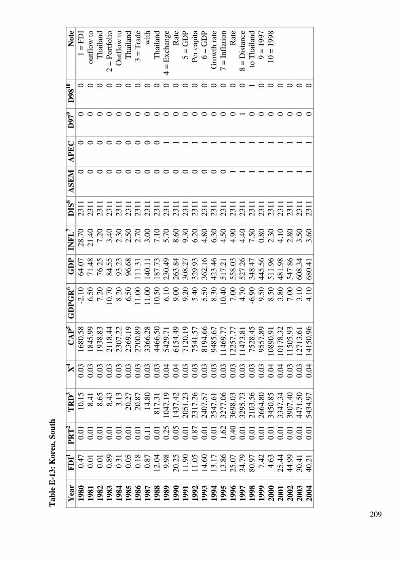
209
Tab
le E
-13:
Kore
a, S
ou
th
Yea
r F
DI1
P
RT
2
TR
D3
X4
CA
P5
GD
PG
R6
GD
P
INF
L7
DIS
8
AS
EM
A
PE
C
D97
9
D98
10
Note
1980
0.4
7
0.0
1
10.1
5
0.0
3
1680.5
8
-2.1
0
64.0
7
28.7
0
2311
0
0
0
0
1 =
FD
I
1981
0.0
1
0.0
1
8.4
1
0.0
3
1845.9
9
6.5
0
71.4
8
21.4
0
2311
0
0
0
0
outf
low
to
1982
0.0
1
0.0
1
8.6
5
0.0
3
1938.8
3
7.2
0
76.2
5
7.2
0
2311
0
0
0
0
Thai
land
1983
0.8
9
0.0
1
8.4
3
0.0
3
2118.4
4
10.7
0
84.5
5
3.4
0
2311
0
0
0
0
2 =
Port
foli
o
1984
0.3
1
0.0
1
3.1
3
0.0
3
2307.2
2
8.2
0
93.2
3
2.3
0
2311
0
0
0
0
Outf
low
to
1985
0.0
5
0.0
1
20.2
7
0.0
3
2369.1
9
6.5
0
96.6
8
2.5
0
2311
0
0
0
0
Thai
land
1986
0.1
8
0.0
1
20.8
7
0.0
3
2700.8
9
11.0
0
111.3
1
2.7
0
2311
0
0
0
0
3 =
Tra
de
1987
0.8
7
0.1
1
14.8
0
0.0
3
3366.2
8
11.0
0
140.1
1
3.0
0
2311
0
0
0
0
wit
h
1988
12.0
4
0.0
1
817.3
1
0.0
3
4466.5
0
10.5
0
187.7
3
7.1
0
2311
0
0
0
0
Thai
land
1989
9.9
8
0.2
5
1047.1
9
0.0
4
5429.7
1
6.1
0
230.4
9
5.7
0
2311
0
1
0
0
4 =
Ex
chan
ge
1990
20.2
5
0.0
5
1437.4
2
0.0
4
6154.4
9
9.0
0
263.8
4
8.6
0
2311
0
1
0
0
Rat
e
1991
11.9
0
0.0
1
2051.2
3
0.0
3
7120.1
9
9.2
0
308.2
7
9.3
0
2311
0
1
0
0
5 =
GD
P
1992
11.0
5
0.8
7
2317.2
6
0.0
3
7541.5
7
5.4
0
329.9
3
6.2
0
2311
0
1
0
0
Per
cap
ita
1993
14.6
0
0.0
1
2407.5
7
0.0
3
8194.6
6
5.5
0
362.1
6
4.8
0
2311
0
1
0
0
6 =
GD
P
1994
13.1
7
0.0
1
2547.6
1
0.0
3
9485.6
7
8.3
0
423.4
6
6.3
0
2311
0
1
0
0
Gro
wth
rat
e
1995
13.8
6
1.6
2
3277.0
6
0.0
3
11469.7
7
10.4
0
517.2
1
4.5
0
2311
0
1
0
0
7 =
Infl
atio
n
1996
25.0
7
0.4
0
3698.0
3
0.0
3
12257.7
7
7.0
0
558.0
3
4.9
0
2311
1
1
0
0
Rat
e
1997
34.7
9
0.0
1
3295.7
3
0.0
3
11473.8
1
4.7
0
527.2
6
4.4
0
2311
1
1
1
0
8 =
Dis
tance
1998
80.9
7
0.0
1
2103.5
6
0.0
3
7528.4
5
-6.9
0
348.4
7
7.5
0
2311
1
1
0
1
to T
hai
land
1999
7.4
2
0.0
1
2664.8
0
0.0
3
9557.8
9
9.5
0
445.5
6
0.8
0
2311
1
1
0
0
9 =
1997
2000
4.6
3
0.0
1
3450.8
5
0.0
4
10890.9
1
8.5
0
511.9
6
2.3
0
2311
1
1
0
0
10 =
1998
2001
25.4
4
0.0
1
3347.3
4
0.0
4
10178.3
2
3.8
0
481.9
8
4.1
0
2311
1
1
0
0
2002
44.9
9
0.0
1
3907.4
0
0.0
3
11505.9
3
7.0
0
547.8
6
2.8
0
2311
1
1
0
0
2003
30.4
1
0.0
1
4471.5
0
0.0
3
12713.6
1
3.1
0
608.3
4
3.5
0
2311
1
1
0
0
2004
40.2
1
0.0
1
5434.9
7
0.0
4
14150.9
6
4.1
0
680.4
1
3.6
0
2311
1
1
0
0
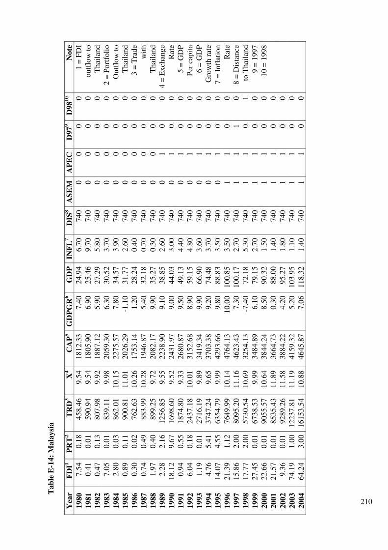
210
Tab
le E
-14:
Mala
ysi
a
Yea
r F
DI1
P
RT
2
TR
D3
X4
CA
P5
GD
PG
R6
GD
P
INF
L7
DIS
8
AS
EM
A
PE
C
D97
9
D98
10
Note
1980
7.5
4
0.1
8
458.4
6
9.5
4
1812.3
3
7.4
0
24.9
4
6.7
0
740
0
0
0
0
1 =
FD
I
1981
0.4
1
0.0
1
590.9
4
9.5
4
1805.9
0
6.9
0
25.4
6
9.7
0
740
0
0
0
0
outf
low
to
1982
0.4
7
0.1
3
807.9
8
9.9
2
1887.1
2
5.9
0
27.2
9
5.8
0
740
0
0
0
0
Thai
land
1983
7.0
5
0.0
1
839.1
1
9.9
8
2059.3
0
6.3
0
30.5
2
3.7
0
740
0
0
0
0
2 =
Port
foli
o
1984
2.8
0
0.0
3
862.0
1
10.1
5
2275.5
7
7.8
0
34.5
7
3.9
0
740
0
0
0
0
Outf
low
to
1985
0.8
9
0.1
1
900.8
1
11.0
1
2026.2
9
-1.1
0
31.7
7
2.6
0
740
0
0
0
0
Thai
land
1986
0.3
0
0.0
2
762.6
3
10.2
6
1753.1
4
1.2
0
28.2
4
0.4
0
740
0
0
0
0
3 =
Tra
de
1987
0.7
4
0.4
9
883.9
9
10.2
8
1946.8
7
5.4
0
32.1
8
0.7
0
740
0
0
0
0
wit
h
1988
1.9
7
0.4
0
899.2
5
9.7
2
2082.1
7
9.9
0
35.2
7
0.3
0
740
0
0
0
0
Thai
land
1989
2.2
8
2.1
6
1256.8
5
9.5
5
2238.9
0
9.1
0
38.8
5
2.6
0
740
0
1
0
0
4 =
Ex
chan
ge
1990
18.1
2
9.6
7
1698.6
0
9.5
2
2431.9
7
9.0
0
44.0
3
3.0
0
740
0
1
0
0
Rat
e
1991
0.9
4
0.5
5
1874.8
0
9.3
3
2680.8
7
9.5
0
49.1
3
4.4
0
740
0
1
0
0
5 =
GD
P
1992
6.0
4
0.1
8
2437.1
8
10.0
1
3152.6
8
8.9
0
59.1
5
4.8
0
740
0
1
0
0
Per
cap
ita
1993
1.1
9
0.0
1
2716.1
9
9.8
9
3419.3
4
9.9
0
66.9
0
3.6
0
740
0
1
0
0
6 =
GD
P
1994
4.7
6
5.4
1
3747.2
4
9.6
5
3703.3
8
9.2
0
74.4
8
3.7
0
740
0
1
0
0
Gro
wth
rat
e
1995
14.0
7
4.5
5
6354.7
9
9.9
9
4293.6
6
9.8
0
88.8
3
3.5
0
740
0
1
0
0
7 =
Infl
atio
n
1996
21.3
9
1.1
2
7649.9
9
10.1
4
4764.1
3
10.0
0
100.8
5
3.5
0
740
1
1
0
0
Rat
e
1997
15.8
6
2.0
0
8095.2
0
11.1
6
4623.4
3
7.3
0
100.1
7
2.7
0
740
1
1
1
0
8 =
Dis
tance
1998
17.7
7
2.0
0
5730.5
4
10.6
9
3254.1
3
-7.4
0
72.1
8
5.3
0
740
1
1
0
1
to T
hai
land
1999
27.4
5
0.0
1
6738.5
3
9.9
9
3484.8
9
6.1
0
79.1
5
2.7
0
740
1
1
0
0
9 =
1997
2000
22.6
6
0.0
1
9055.5
7
10.6
4
3844.2
4
8.5
0
90.3
2
1.5
0
740
1
1
0
0
10 =
1998
2001
21.5
7
0.0
1
8535.4
3
11.8
9
3664.7
3
0.3
0
88.0
0
1.4
0
740
1
1
0
0
2002
9.3
6
0.0
1
9289.2
6
11.5
8
3884.2
2
4.2
0
95.2
7
1.8
0
740
1
1
0
0
2003
74.1
9
1.0
0
12237.8
1
11.1
9
4159.3
2
5.2
0
103.9
5
1.1
0
740
1
1
0
0
2004
64.2
4
3.0
0
16153.5
4
10.8
8
4645.8
7
7.0
6
118.3
2
1.4
0
740
1
1
0
0
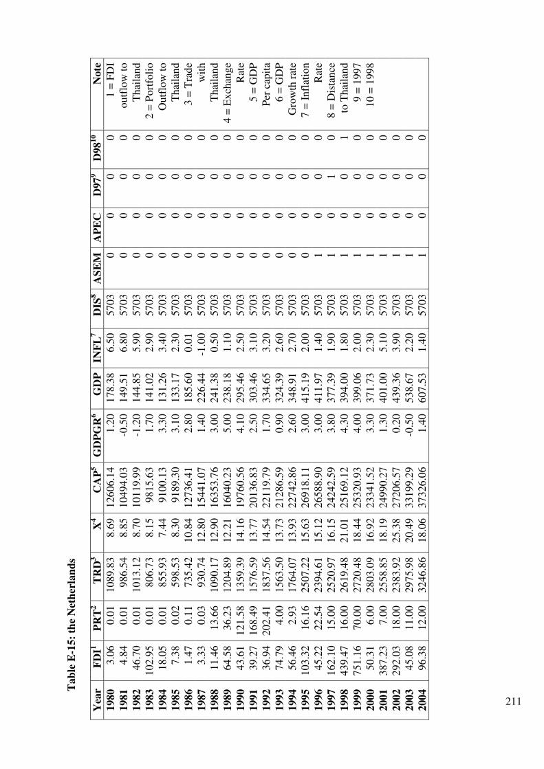
211
Tab
le E
-15:
the
Net
her
lan
ds
Yea
r F
DI1
P
RT
2
TR
D3
X4
CA
P5
GD
PG
R6
GD
P
INF
L7
DIS
8
AS
EM
A
PE
C
D97
9
D98
10
Note
1980
3.0
6
0.0
1
1089.8
3
8.6
9
12606.1
4
1.2
0
178.3
8
6.5
0
5703
0
0
0
0
1 =
FD
I
1981
4.8
4
0.0
1
986.5
4
8.8
5
10494.0
3
-0.5
0
149.5
1
6.8
0
5703
0
0
0
0
outf
low
to
1982
46.7
0
0.0
1
1013.1
2
8.7
0
10119.9
9
-1.2
0
144.8
5
5.9
0
5703
0
0
0
0
Thai
land
1983
102.9
5
0.0
1
806.7
3
8.1
5
9815.6
3
1.7
0
141.0
2
2.9
0
5703
0
0
0
0
2 =
Port
foli
o
1984
18.0
5
0.0
1
855.9
3
7.4
4
9100.1
3
3.3
0
131.2
6
3.4
0
5703
0
0
0
0
Outf
low
to
1985
7.3
8
0.0
2
598.5
3
8.3
0
9189.3
0
3.1
0
133.1
7
2.3
0
5703
0
0
0
0
Thai
land
1986
1.4
7
0.1
1
735.4
2
10.8
4
12736.4
1
2.8
0
185.6
0
0.0
1
5703
0
0
0
0
3 =
Tra
de
1987
3.3
3
0.0
3
930.7
4
12.8
0
15441.0
7
1.4
0
226.4
4
-1.0
0
5703
0
0
0
0
wit
h
1988
11.4
6
13.6
6
1090.1
7
12.9
0
16353.7
6
3.0
0
241.3
8
0.5
0
5703
0
0
0
0
Thai
land
1989
64.5
8
36.2
3
1204.8
9
12.2
1
16040.2
3
5.0
0
238.1
8
1.1
0
5703
0
0
0
0
4 =
Ex
chan
ge
1990
43.6
1
121.5
8
1359.3
9
14.1
6
19760.5
6
4.1
0
295.4
6
2.5
0
5703
0
0
0
0
Rat
e
1991
39.2
7
168.4
9
1576.5
9
13.7
7
20136.8
3
2.5
0
303.4
6
3.1
0
5703
0
0
0
0
5 =
GD
P
1992
36.9
4
202.4
1
1837.5
6
14.5
4
22119.7
9
1.7
0
334.6
5
3.2
0
5703
0
0
0
0
Per
cap
ita
1993
74.7
9
4.0
0
1563.5
0
13.7
3
21286.5
9
0.9
0
324.3
9
2.6
0
5703
0
0
0
0
6 =
GD
P
1994
56.4
6
2.9
3
1764.0
7
13.9
3
22742.8
6
2.6
0
348.9
1
2.7
0
5703
0
0
0
0
Gro
wth
rat
e
1995
103.3
2
16.1
6
2507.2
2
15.6
3
26918.1
1
3.0
0
415.1
9
2.0
0
5703
0
0
0
0
7 =
Infl
atio
n
1996
45.2
2
22.5
4
2394.6
1
15.1
2
26588.9
0
3.0
0
411.9
7
1.4
0
5703
1
0
0
0
Rat
e
1997
162.1
0
15.0
0
2520.9
7
16.1
5
24242.5
9
3.8
0
377.3
9
1.9
0
5703
1
0
1
0
8 =
Dis
tance
1998
439.4
7
16.0
0
2619.4
8
21.0
1
25169.1
2
4.3
0
394.0
0
1.8
0
5703
1
0
0
1
to T
hai
land
1999
751.1
6
70.0
0
2720.4
8
18.4
4
25320.9
3
4.0
0
399.0
6
2.0
0
5703
1
0
0
0
9 =
1997
2000
50.3
1
6.0
0
2803.0
9
16.9
2
23341.5
2
3.3
0
371.7
3
2.3
0
5703
1
0
0
0
10 =
1998
2001
387.2
3
7.0
0
2558.8
5
18.1
9
24990.2
7
1.3
0
401.0
0
5.1
0
5703
1
0
0
0
2002
292.0
3
18.0
0
2383.9
2
25.3
8
27206.5
7
0.2
0
439.3
6
3.9
0
5703
1
0
0
0
2003
45.0
8
11.0
0
2975.9
8
20.4
9
33199.2
9
-0.5
0
538.6
7
2.2
0
5703
1
0
0
0
2004
96.3
8
12.0
0
3246.8
6
18.0
6
37326.0
6
1.4
0
607.5
3
1.4
0
5703
1
0
0
0
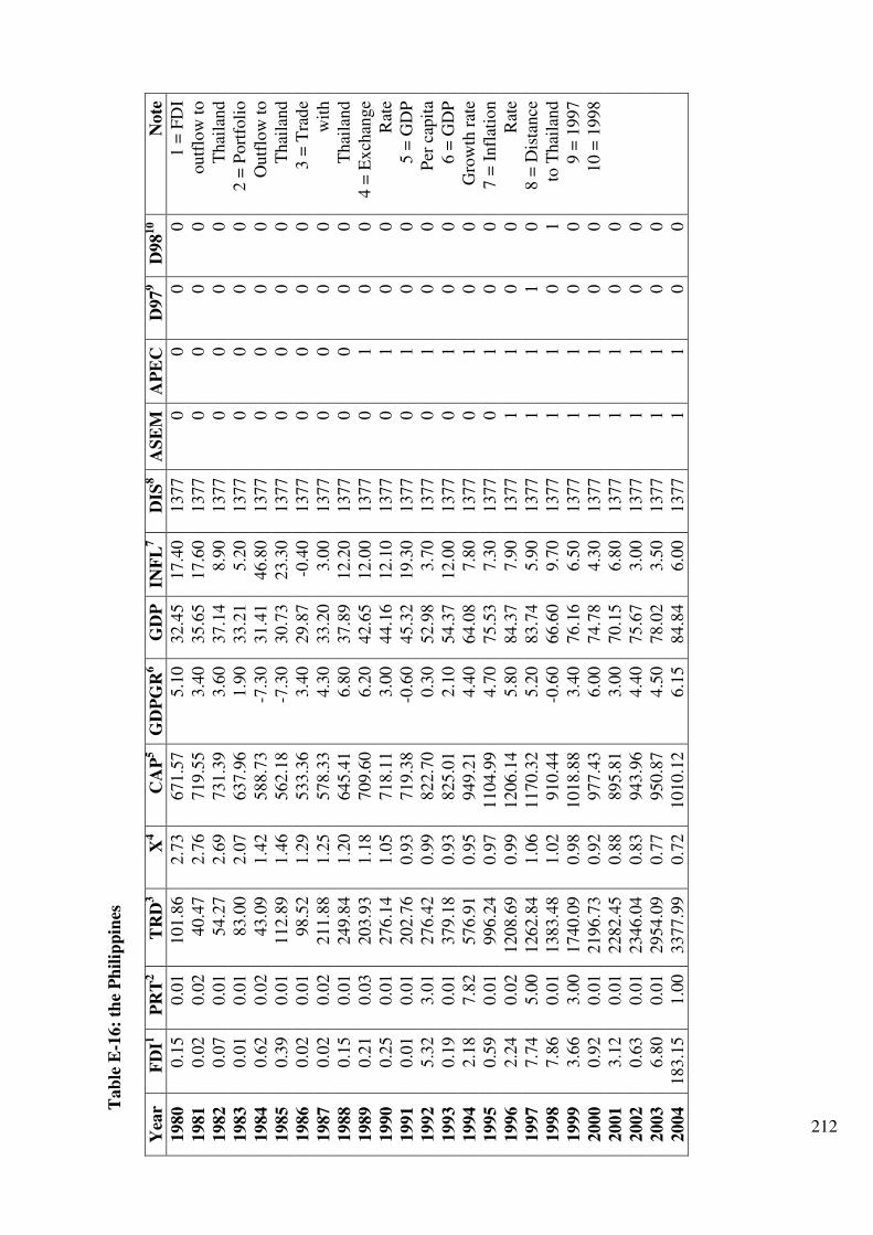
212
Tab
le E
-16:
the
Ph
ilip
pin
es
Yea
r F
DI1
P
RT
2
TR
D3
X4
CA
P5
GD
PG
R6
GD
P
INF
L7
DIS
8
AS
EM
A
PE
C
D97
9
D98
10
Note
1980
0.1
5
0.0
1
101.8
6
2.7
3
671.5
7
5.1
0
32.4
5
17.4
0
1377
0
0
0
0
1 =
FD
I
1981
0.0
2
0.0
2
40.4
7
2.7
6
719.5
5
3.4
0
35.6
5
17.6
0
1377
0
0
0
0
outf
low
to
1982
0.0
7
0.0
1
54.2
7
2.6
9
731.3
9
3.6
0
37.1
4
8.9
0
1377
0
0
0
0
Thai
land
1983
0.0
1
0.0
1
83.0
0
2.0
7
637.9
6
1.9
0
33.2
1
5.2
0
1377
0
0
0
0
2 =
Port
foli
o
1984
0.6
2
0.0
2
43.0
9
1.4
2
588.7
3
-7.3
0
31.4
1
46.8
0
1377
0
0
0
0
Outf
low
to
1985
0.3
9
0.0
1
112.8
9
1.4
6
562.1
8
-7.3
0
30.7
3
23.3
0
1377
0
0
0
0
Thai
land
1986
0.0
2
0.0
1
98.5
2
1.2
9
533.3
6
3.4
0
29.8
7
-0.4
0
1377
0
0
0
0
3 =
Tra
de
1987
0.0
2
0.0
2
211.8
8
1.2
5
578.3
3
4.3
0
33.2
0
3.0
0
1377
0
0
0
0
wit
h
1988
0.1
5
0.0
1
249.8
4
1.2
0
645.4
1
6.8
0
37.8
9
12.2
0
1377
0
0
0
0
Thai
land
1989
0.2
1
0.0
3
203.9
3
1.1
8
709.6
0
6.2
0
42.6
5
12.0
0
1377
0
1
0
0
4 =
Ex
chan
ge
1990
0.2
5
0.0
1
276.1
4
1.0
5
718.1
1
3.0
0
44.1
6
12.1
0
1377
0
1
0
0
Rat
e
1991
0.0
1
0.0
1
202.7
6
0.9
3
719.3
8
-0.6
0
45.3
2
19.3
0
1377
0
1
0
0
5 =
GD
P
1992
5.3
2
3.0
1
276.4
2
0.9
9
822.7
0
0.3
0
52.9
8
3.7
0
1377
0
1
0
0
Per
cap
ita
1993
0.1
9
0.0
1
379.1
8
0.9
3
825.0
1
2.1
0
54.3
7
12.0
0
1377
0
1
0
0
6 =
GD
P
1994
2.1
8
7.8
2
576.9
1
0.9
5
949.2
1
4.4
0
64.0
8
7.8
0
1377
0
1
0
0
Gro
wth
rat
e
1995
0.5
9
0.0
1
996.2
4
0.9
7
1104.9
9
4.7
0
75.5
3
7.3
0
1377
0
1
0
0
7 =
Infl
atio
n
1996
2.2
4
0.0
2
1208.6
9
0.9
9
1206.1
4
5.8
0
84.3
7
7.9
0
1377
1
1
0
0
Rat
e
1997
7.7
4
5.0
0
1262.8
4
1.0
6
1170.3
2
5.2
0
83.7
4
5.9
0
1377
1
1
1
0
8 =
Dis
tance
1998
7.8
6
0.0
1
1383.4
8
1.0
2
910.4
4
-0.6
0
66.6
0
9.7
0
1377
1
1
0
1
to T
hai
land
1999
3.6
6
3.0
0
1740.0
9
0.9
8
1018.8
8
3.4
0
76.1
6
6.5
0
1377
1
1
0
0
9 =
1997
2000
0.9
2
0.0
1
2196.7
3
0.9
2
977.4
3
6.0
0
74.7
8
4.3
0
1377
1
1
0
0
10 =
1998
2001
3.1
2
0.0
1
2282.4
5
0.8
8
895.8
1
3.0
0
70.1
5
6.8
0
1377
1
1
0
0
2002
0.6
3
0.0
1
2346.0
4
0.8
3
943.9
6
4.4
0
75.6
7
3.0
0
1377
1
1
0
0
2003
6.8
0
0.0
1
2954.0
9
0.7
7
950.8
7
4.5
0
78.0
2
3.5
0
1377
1
1
0
0
2004
183.1
5
1.0
0
3377.9
9
0.7
2
1010.1
2
6.1
5
84.8
4
6.0
0
1377
1
1
0
0
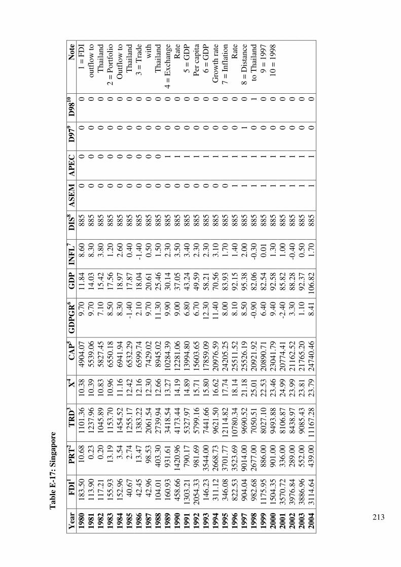
213
Tab
le E
-17:
Sin
gap
ore
Yea
r F
DI1
P
RT
2
TR
D3
X4
CA
P5
GD
PG
R6
GD
P
INF
L7
DIS
8
AS
EM
A
PE
C
D97
9
D98
10
Note
1980
183.5
0
10.6
8
1101.3
6
10.3
8
4904.0
7
9.7
0
11.8
4
8.6
0
885
0
0
0
0
1 =
FD
I
1981
113.9
0
0.2
3
1237.9
6
10.3
9
5539.0
6
9.7
0
14.0
3
8.3
0
885
0
0
0
0
outf
low
to
1982
117.2
1
0.2
0
1045.8
9
10.8
3
5827.4
5
7.1
0
15.4
2
3.8
0
885
0
0
0
0
Thai
land
1983
155.9
3
13.1
9
1153.7
0
10.9
6
6550.1
8
8.5
0
17.5
6
1.2
0
885
0
0
0
0
2 =
Port
foli
o
1984
152.9
6
3.5
4
1454.5
2
11.1
6
6941.9
4
8.3
0
18.9
7
2.6
0
885
0
0
0
0
Outf
low
to
1985
40.6
7
2.7
4
1255.1
7
12.4
2
6532.2
9
-1.4
0
17.8
7
0.4
0
885
0
0
0
0
Thai
land
1986
42.4
5
13.4
7
1383.2
2
12.1
6
6599.7
4
2.1
0
18.0
4
-1.4
0
885
0
0
0
0
3 =
Tra
de
1987
42.9
6
98.5
3
2061.5
4
12.3
0
7429.0
2
9.7
0
20.6
1
0.5
0
885
0
0
0
0
wit
h
1988
104.0
1
403.3
0
2739.9
4
12.6
6
8945.0
2
11.3
0
25.4
6
1.5
0
885
0
0
0
0
Thai
land
1989
160.9
3
931.6
1
3418.5
4
13.2
7
10284.3
9
9.9
0
30.1
4
2.3
0
885
0
1
0
0
4 =
Ex
chan
ge
1990
458.6
6
1420.9
6
4173.4
4
14.1
9
12281.0
6
9.0
0
37.0
5
3.5
0
885
0
1
0
0
Rat
e
1991
1303.2
1
790.1
7
5327.9
7
14.8
9
13994.8
0
6.8
0
43.2
4
3.4
0
885
0
1
0
0
5 =
GD
P
1992
2054.3
3
981.6
9
5799.1
6
15.7
1
15603.6
5
6.7
0
49.5
9
2.3
0
885
0
1
0
0
Per
cap
ita
1993
146.2
3
3544.0
0
7441.6
6
15.8
0
17859.0
9
12.3
0
58.2
1
2.3
0
885
0
1
0
0
6 =
GD
P
1994
311.1
2
2668.7
3
9621.5
0
16.6
2
20976.5
9
11.4
0
70.5
6
3.1
0
885
0
1
0
0
Gro
wth
rat
e
1995
346.0
8
3701.7
7
12114.8
2
17.7
4
24205.2
5
8.0
0
83.9
3
1.7
0
885
0
1
0
0
7 =
Infl
atio
n
1996
822.5
3
3523.6
9
10780.3
4
18.1
4
25511.5
2
8.1
0
92.1
5
1.4
0
885
1
1
0
0
Rat
e
1997
904.0
4
9014.0
0
9690.5
2
21.1
8
25526.1
9
8.5
0
95.3
8
2.0
0
885
1
1
1
0
8 =
Dis
tance
1998
982.6
8
2677.0
0
7050.5
1
25.0
1
20921.9
2
-0.9
0
82.0
6
-0.3
0
885
1
1
0
1
to T
hai
land
1999
1175.9
5
886.0
0
8027.1
0
22.5
3
20890.7
1
6.4
0
82.5
4
0.0
1
885
1
1
0
0
9 =
1997
2000
1504.3
5
901.0
0
9493.8
8
23.4
6
23041.7
9
9.4
0
92.5
8
1.3
0
885
1
1
0
0
10 =
1998
2001
3570.7
2
336.0
0
8106.8
7
24.9
9
20774.4
1
-2.4
0
85.8
2
1.0
0
885
1
1
0
0
2002
3976.8
4
289.0
0
8438.9
7
23.9
9
21162.5
2
3.3
0
88.2
8
-0.4
0
885
1
1
0
0
2003
3886.9
6
552.0
0
9085.4
3
23.8
1
21765.2
0
1.1
0
92.3
7
0.5
0
885
1
1
0
0
2004
3114.6
4
439.0
0
11167.2
8
23.7
9
24740.4
6
8.4
1
106.8
2
1.7
0
885
1
1
0
0
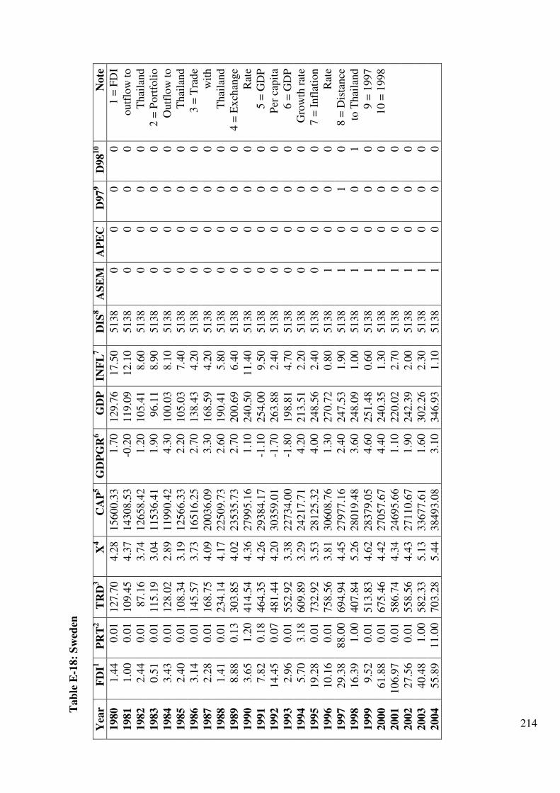
214
Tab
le E
-18:
Sw
eden
Yea
r F
DI1
P
RT
2
TR
D3
X4
CA
P5
GD
PG
R6
GD
P
INF
L7
DIS
8
AS
EM
A
PE
C
D97
9
D98
10
Note
1980
1.4
4
0.0
1
127.7
0
4.2
8
15600.3
3
1.7
0
129.7
6
17.5
0
5138
0
0
0
0
1 =
FD
I
1981
1.0
0
0.0
1
109.4
5
4.3
7
14308.5
3
-0.2
0
119.0
9
12.1
0
5138
0
0
0
0
outf
low
to
1982
2.4
4
0.0
1
87.1
6
3.7
4
12658.4
2
1.2
0
105.4
1
8.6
0
5138
0
0
0
0
Thai
land
1983
0.5
1
0.0
1
115.1
9
3.0
4
11536.4
1
1.9
0
96.1
1
8.9
0
5138
0
0
0
0
2 =
Port
foli
o
1984
3.4
3
0.0
1
128.0
2
2.8
9
11990.4
2
4.3
0
100.0
3
8.1
0
5138
0
0
0
0
Outf
low
to
1985
2.4
0
0.0
1
108.3
4
3.1
9
12566.3
3
2.2
0
105.0
3
7.4
0
5138
0
0
0
0
Thai
land
1986
3.1
4
0.0
1
145.5
7
3.7
3
16516.2
5
2.7
0
138.4
3
4.2
0
5138
0
0
0
0
3 =
Tra
de
1987
2.2
8
0.0
1
168.7
5
4.0
9
20036.0
9
3.3
0
168.5
9
4.2
0
5138
0
0
0
0
wit
h
1988
1.4
1
0.0
1
234.1
4
4.1
7
22509.7
3
2.6
0
190.4
1
5.8
0
5138
0
0
0
0
Thai
land
1989
8.8
8
0.1
3
303.8
5
4.0
2
23535.7
3
2.7
0
200.6
9
6.4
0
5138
0
0
0
0
4 =
Ex
chan
ge
1990
3.6
5
1.2
0
414.5
4
4.3
6
27995.1
6
1.1
0
240.5
0
11.4
0
5138
0
0
0
0
Rat
e
1991
7.8
2
0.1
8
464.3
5
4.2
6
29384.1
7
-1.1
0
254.0
0
9.5
0
5138
0
0
0
0
5 =
GD
P
1992
14.4
5
0.0
7
481.4
4
4.2
0
30359.0
1
-1.7
0
263.8
8
2.4
0
5138
0
0
0
0
Per
cap
ita
1993
2.9
6
0.0
1
552.9
2
3.3
8
22734.0
0
-1.8
0
198.8
1
4.7
0
5138
0
0
0
0
6 =
GD
P
1994
5.7
0
3.1
8
609.8
9
3.2
9
24217.7
1
4.2
0
213.5
1
2.2
0
5138
0
0
0
0
Gro
wth
rat
e
1995
19.2
8
0.0
1
732.9
2
3.5
3
28125.3
2
4.0
0
248.5
6
2.4
0
5138
0
0
0
0
7 =
Infl
atio
n
1996
10.1
6
0.0
1
758.5
6
3.8
1
30608.7
6
1.3
0
270.7
2
0.8
0
5138
1
0
0
0
Rat
e
1997
29.3
8
88.0
0
694.9
4
4.4
5
27977.1
6
2.4
0
247.5
3
1.9
0
5138
1
0
1
0
8 =
Dis
tance
1998
16.3
9
1.0
0
407.8
4
5.2
6
28019.4
8
3.6
0
248.0
9
1.0
0
5138
1
0
0
1
to T
hai
land
1999
9.5
2
0.0
1
513.8
3
4.6
2
28379.0
5
4.6
0
251.4
8
0.6
0
5138
1
0
0
0
9 =
1997
2000
61.8
8
0.0
1
675.4
6
4.4
2
27057.6
7
4.4
0
240.3
5
1.3
0
5138
1
0
0
0
10 =
1998
2001
106.9
7
0.0
1
586.7
4
4.3
4
24695.6
6
1.1
0
220.0
2
2.7
0
5138
1
0
0
0
2002
27.5
6
0.0
1
558.5
6
4.4
3
27110.6
7
1.9
0
242.3
9
2.0
0
5138
1
0
0
0
2003
40.4
8
1.0
0
582.3
3
5.1
3
33677.6
1
1.6
0
302.2
6
2.3
0
5138
1
0
0
0
2004
55.8
9
11.0
0
703.2
8
5.4
4
38493.0
8
3.1
0
346.9
3
1.1
0
5138
1
0
0
0
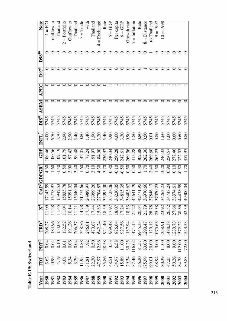
215
Tab
le E
-19:
Sw
itze
rlan
d
Yea
r F
DI1
P
RT
2
TR
D3
X4
CA
P5 G
DP
GR
6
GD
P
INF
L7
DIS
8
AS
EM
A
PE
C
D97
9
D98
10
Note
1980
3.6
2
0.0
4
208.2
7
11.0
9
17143.5
9
4.6
0
109.4
6
4.0
0
5745
0
0
0
0
1 =
FD
I
1981
0.9
9
0.0
4
184.9
6
11.2
8
15778.9
7
1.6
0
100.5
6
6.5
0
5745
0
0
0
0
outf
low
to
1982
4.1
9
0.1
0
154.0
8
11.4
5
15942.5
3
-1.4
0
102.1
9
5.7
0
5745
0
0
0
0
Thai
land
1983
4.0
8
0.0
1
182.5
2
11.0
4
15835.7
8
0.5
0
101.7
9
2.9
0
5745
0
0
0
0
2 =
Port
foli
o
1984
5.3
4
0.0
6
191.2
6
10.1
4
15091.0
2
3.0
0
97.4
3
2.9
0
5745
0
0
0
0
Outf
low
to
1985
3.2
9
0.0
4
206.3
7
11.2
1
15340.0
4
3.4
0
99.4
8
3.4
0
5745
0
0
0
0
Thai
land
1986
11.9
5
0.8
8
248.7
6
14.7
8
21774.6
6
1.6
0
142.0
5
0.8
0
5745
0
0
0
0
3 =
Tra
de
1987
31.8
1
1.9
2
286.0
1
17.3
9
26989.9
7
0.7
0
177.2
4
1.4
0
5745
0
0
0
0
wit
h
1988
22.3
0
0.5
0
470.6
7
17.4
4
28999.2
6
3.1
0
191.9
7
1.9
0
5745
0
0
0
0
Thai
land
1989
47.9
7
12.9
6
642.2
4
15.8
3
27704.8
7
4.3
0
184.9
0
3.2
0
5745
0
0
0
0
4 =
Ex
chan
ge
1990
35.8
6
28.5
8
921.4
0
18.5
9
35095.0
0
3.7
0
236.9
2
5.4
0
5745
0
0
0
0
Rat
e
1991
48.5
1
3.5
3
969.4
8
17.9
7
35123.0
6
-0.8
0
240.3
4
5.9
0
5745
0
1
0
0
5 =
GD
P
1992
34.9
7
6.5
8
876.0
4
18.0
7
36230.0
5
-0.1
0
250.2
8
4.0
0
5745
0
1
0
0
Per
cap
ita
1993
15.8
9
11.0
0
927.5
6
17.2
4
34815.3
5
-0.5
0
242.6
1
3.3
0
5745
0
1
0
0
6 =
GD
P
1994
29.3
4
30.2
5
1137.9
4
18.5
3
38403.6
2
0.5
0
269.5
6
0.9
0
5745
0
1
0
0
Gro
wth
rat
e
1995
37.4
6
116.0
2
1471.1
5
21.2
2
44641.7
9
0.5
0
315.2
8
1.8
0
5745
0
1
0
0
7 =
Infl
atio
n
1996
56.2
0
81.5
7
5945.3
3
20.6
4
42771.9
5
0.3
0
302.8
8
0.8
0
5745
0
1
0
0
Rat
e
1997
175.9
9
83.0
0
1290.4
7
21.7
9
36970.6
6
1.7
0
262.3
6
0.5
0
5745
0
1
1
0
8 =
Dis
tance
1998
199.0
1
20.0
0
1120.1
2
28.7
8
37846.1
7
2.4
0
269.6
0
0.0
1
5745
0
1
0
1
to T
hai
land
1999
68.9
4
3.0
0
1075.6
3
25.3
8
37020.2
5
1.5
0
265.2
3
0.8
0
5745
0
1
0
0
9 =
1997
2000
80.3
9
11.0
0
1258.9
1
23.9
2
34263.2
3
3.2
0
246.3
2
1.6
0
5745
0
1
0
0
10 =
1998
2001
47.2
5
8.0
0
1488.3
8
26.5
2
34748.2
4
0.9
0
250.5
7
1.0
0
5745
0
1
0
0
2002
50.2
6
9.0
0
1230.7
3
27.6
6
38374.6
1
0.1
0
277.4
6
0.6
0
5745
0
1
0
0
2003
84.7
8
112.0
0
1572.2
2
30.8
6
44438.5
9
-0.5
0
322.0
3
0.6
0
5745
0
1
0
0
2004
89.8
3
72.0
0
1543.5
3
32.3
9
49300.0
4
1.7
0
357.9
7
0.8
0
5745
0
1
0
0
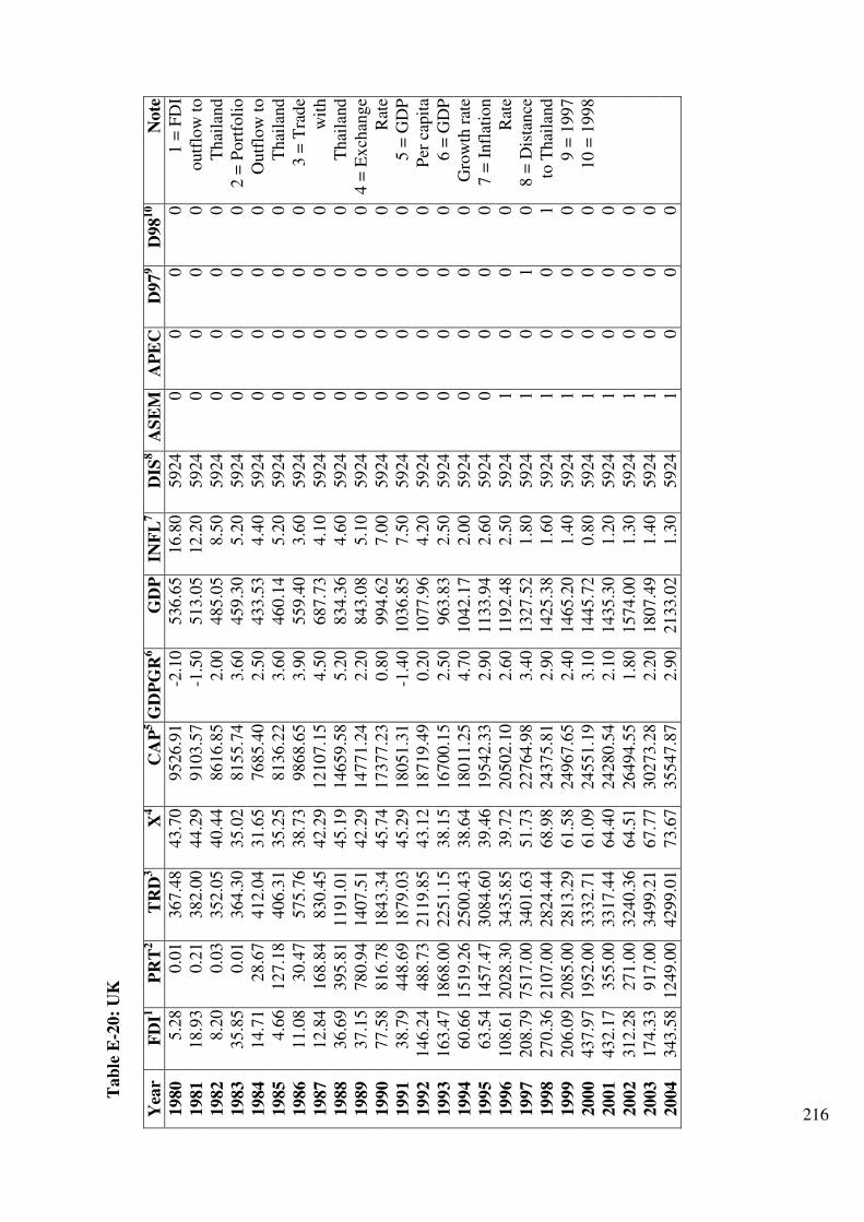
216
Tab
le E
-20:
UK
Yea
r F
DI1
P
RT
2
TR
D3
X4
CA
P5 G
DP
GR
6
GD
P
INF
L7
DIS
8
AS
EM
A
PE
C
D97
9
D98
10
Note
1980
5.2
8
0.0
1
367.4
8
43.7
0
9526.9
1
-2.1
0
536.6
5
16.8
0
5924
0
0
0
0
1 =
FD
I
1981
18.9
3
0.2
1
382.0
0
44.2
9
9103.5
7
-1.5
0
513.0
5
12.2
0
5924
0
0
0
0
outf
low
to
1982
8.2
0
0.0
3
352.0
5
40.4
4
8616.8
5
2.0
0
485.0
5
8.5
0
5924
0
0
0
0
Thai
land
1983
35.8
5
0.0
1
364.3
0
35.0
2
8155.7
4
3.6
0
459.3
0
5.2
0
5924
0
0
0
0
2 =
Port
foli
o
1984
14.7
1
28.6
7
412.0
4
31.6
5
7685.4
0
2.5
0
433.5
3
4.4
0
5924
0
0
0
0
Outf
low
to
1985
4.6
6
127.1
8
406.3
1
35.2
5
8136.2
2
3.6
0
460.1
4
5.2
0
5924
0
0
0
0
Thai
land
1986
11.0
8
30.4
7
575.7
6
38.7
3
9868.6
5
3.9
0
559.4
0
3.6
0
5924
0
0
0
0
3 =
Tra
de
1987
12.8
4
168.8
4
830.4
5
42.2
9
12107.1
5
4.5
0
687.7
3
4.1
0
5924
0
0
0
0
wit
h
1988
36.6
9
395.8
1
1191.0
1
45.1
9
14659.5
8
5.2
0
834.3
6
4.6
0
5924
0
0
0
0
Thai
land
1989
37.1
5
780.9
4
1407.5
1
42.2
9
14771.2
4
2.2
0
843.0
8
5.1
0
5924
0
0
0
0
4 =
Ex
chan
ge
1990
77.5
8
816.7
8
1843.3
4
45.7
4
17377.2
3
0.8
0
994.6
2
7.0
0
5924
0
0
0
0
Rat
e
1991
38.7
9
448.6
9
1879.0
3
45.2
9
18051.3
1
-1.4
0
1036.8
5
7.5
0
5924
0
0
0
0
5 =
GD
P
1992
146.2
4
488.7
3
2119.8
5
43.1
2
18719.4
9
0.2
0
1077.9
6
4.2
0
5924
0
0
0
0
Per
cap
ita
1993
163.4
7
1868.0
0
2251.1
5
38.1
5
16700.1
5
2.5
0
963.8
3
2.5
0
5924
0
0
0
0
6 =
GD
P
1994
60.6
6
1519.2
6
2500.4
3
38.6
4
18011.2
5
4.7
0
1042.1
7
2.0
0
5924
0
0
0
0
Gro
wth
rat
e
1995
63.5
4
1457.4
7
3084.6
0
39.4
6
19542.3
3
2.9
0
1133.9
4
2.6
0
5924
0
0
0
0
7 =
Infl
atio
n
1996
108.6
1
2028.3
0
3435.8
5
39.7
2
20502.1
0
2.6
0
1192.4
8
2.5
0
5924
1
0
0
0
Rat
e
1997
208.7
9
7517.0
0
3401.6
3
51.7
3
22764.9
8
3.4
0
1327.5
2
1.8
0
5924
1
0
1
0
8 =
Dis
tance
1998
270.3
6
2107.0
0
2824.4
4
68.9
8
24375.8
1
2.9
0
1425.3
8
1.6
0
5924
1
0
0
1
to T
hai
land
1999
206.0
9
2085.0
0
2813.2
9
61.5
8
24967.6
5
2.4
0
1465.2
0
1.4
0
5924
1
0
0
0
9 =
1997
2000
437.9
7
1952.0
0
3332.7
1
61.0
9
24551.1
9
3.1
0
1445.7
2
0.8
0
5924
1
0
0
0
10 =
1998
2001
432.1
7
355.0
0
3317.4
4
64.4
0
24280.5
4
2.1
0
1435.3
0
1.2
0
5924
1
0
0
0
2002
312.2
8
271.0
0
3240.3
6
64.5
1
26494.5
5
1.8
0
1574.0
0
1.3
0
5924
1
0
0
0
2003
174.3
3
917.0
0
3499.2
1
67.7
7
30273.2
8
2.2
0
1807.4
9
1.4
0
5924
1
0
0
0
2004
343.5
8
1249.0
0
4299.0
1
73.6
7
35547.8
7
2.9
0
2133.0
2
1.3
0
5924
1
0
0
0
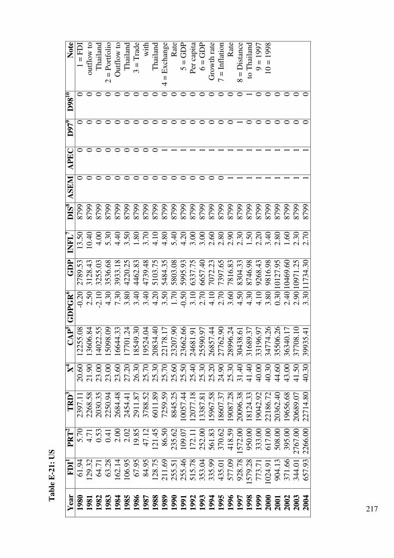
217
Tab
le E
-21:
US
Yea
r F
DI1
P
RT
2
TR
D3
X4
CA
P5 G
DP
GR
6
GD
P
INF
L7
DIS
8
AS
EM
A
PE
C
D97
9
D98
10
Note
1980
61.9
4
5.7
0
2397.1
1
20.6
0
12255.0
8
-0.2
0
2789.5
3
13.5
0
8799
0
0
0
0
1 =
FD
I
1981
129.3
2
4.7
1
2268.5
8
21.9
0
13606.8
4
2.5
0
3128.4
3
10.4
0
8799
0
0
0
0
outf
low
to
1982
64.7
1
0.5
3
2030.3
5
23.0
0
14022.5
5
-2.1
0
3255.0
3
4.0
0
8799
0
0
0
0
Thai
land
1983
63.2
8
0.4
1
2250.9
4
23.0
0
15098.0
9
4.3
0
3536.6
8
5.3
0
8799
0
0
0
0
2 =
Port
foli
o
1984
162.1
4
2.0
0
2684.4
8
23.6
0
16644.3
3
7.3
0
3933.1
8
4.4
0
8799
0
0
0
0
Outf
low
to
1985
106.9
5
2.0
2
2454.4
1
27.2
0
17701.2
4
3.8
0
4220.2
5
3.5
0
8799
0
0
0
0
Thai
land
1986
67.9
5
19.8
5
2911.8
7
26.3
0
18549.3
0
3.4
0
4462.8
3
1.8
0
8799
0
0
0
0
3 =
Tra
de
1987
84.9
5
47.1
2
3788.5
2
25.7
0
19524.0
4
3.4
0
4739.4
8
3.7
0
8799
0
0
0
0
wit
h
1988
128.7
5
121.4
5
6011.8
9
25.3
0
20834.4
0
4.2
0
5103.7
5
4.1
0
8799
0
0
0
0
Thai
land
1989
211.6
9
86.5
0
7259.5
9
25.7
0
22178.1
7
3.5
0
5484.3
5
4.8
0
8799
0
1
0
0
4 =
Ex
chan
ge
1990
255.5
1
235.6
2
8845.2
5
25.6
0
23207.9
0
1.7
0
5803.0
8
5.4
0
8799
0
1
0
0
Rat
e
1991
255.4
6
109.0
7
10057.4
4
25.5
0
23662.6
6
-0.5
0
5995.9
3
4.2
0
8799
0
1
0
0
5 =
GD
P
1992
515.7
8
172.1
1
12077.1
8
25.4
0
24681.9
1
3.1
0
6337.7
5
3.0
0
8799
0
1
0
0
Per
cap
ita
1993
353.0
4
252.0
0
13387.8
1
25.3
0
25590.9
7
2.7
0
6657.4
0
3.0
0
8799
0
1
0
0
6 =
GD
P
1994
335.9
9
561.8
3
15967.5
8
25.2
0
26857.4
4
4.1
0
7072.2
3
2.6
0
8799
0
1
0
0
Gro
wth
rat
e
1995
435.0
1
370.6
2
18607.3
7
24.9
0
27762.9
0
2.7
0
7397.6
5
2.8
0
8799
0
1
0
0
7 =
Infl
atio
n
1996
577.0
9
418.5
9
19087.2
8
25.3
0
28996.2
4
3.6
0
7816.8
3
2.9
0
8799
1
1
0
0
Rat
e
1997
928.7
8
1572.0
0
20096.3
8
31.4
0
30438.6
1
4.5
0
8304.3
3
2.3
0
8799
1
1
1
0
8 =
Dis
tance
1998
1579.2
8
950.0
0
18124.3
3
41.4
0
31689.3
7
4.3
0
8746.9
8
1.5
0
8799
1
1
0
1
to T
hai
land
1999
773.7
1
333.0
0
19042.9
2
40.0
0
33196.9
7
4.1
0
9268.4
3
2.2
0
8799
1
1
0
0
9 =
1997
2000
1024.9
1
617.0
0
22186.7
2
40.3
0
34774.2
6
3.8
0
9816.9
8
3.4
0
8799
1
1
0
0
10 =
1998
2001
904.1
3
508.0
0
20362.4
0
44.6
0
35506.2
6
0.3
0 1
0127.9
5
2.8
0
8799
1
1
0
0
2002
371.6
6
395.0
0
19656.6
8
43.0
0
36340.1
7
2.4
0 1
0469.6
0
1.6
0
8799
1
1
0
0
2003
344.0
1
2767.0
0
20689.0
7
41.5
0
37708.1
0
2.9
0 1
0971.2
5
2.3
0
8799
1
1
0
0
2004
657.9
3
2266.0
0
22714.8
0
40.3
0
39935.4
1
3.3
0 1
1734.3
0
2.7
0
8799
1
1
0
0