determinants of inflation in india: an econometric analysis

WorldWide Indexing, Abstracting and Readership. Peer Reviewed- Refereed International Publication available at http://thescholedge.org ©Scholedge R&D Center

1

SCHOLEDGE INTERNATIONAL JOURNAL OF MANAGEMENT & DEVELOPMENT Vol.2, Issue 8 ISSN 2394-3378 Archives available at http://thescholedge.org

DETERMINANTS OF INFLATION IN INDIA: AN ECONOMETRIC ANALYSIS

Dr. SWAMI P SAXENA1

Ms. ARCHANA SINGH2

1Professor, Department of Applied Business Economics, Dayalbagh Educational Institute (Deemed University)

Agra, India

2Research Scholar, Department of Applied Business Economics, Dayalbagh Educational Institute (Deemed

University) Agra, India

ABSTRACT

Inflation is a continual increase in general price level of goods and services in an economy over a period of

time. It is caused by many factors, important among them are excess of demand of goods and services over

supply, macroeconomic performance, money supply, economic policies implications, environmental factors

etc. A number of researchers in the past made attempts to identify determinants of inflation and to investigate

the impact of identified variables on inflation in European and also in some Asian economies. But, in context of

India, not many studies can be traced in the literature. The purpose of this paper is to shed some light on the

impact of selected variables on inflation in India. The paper considers CPI (Consumer Price Index) inflation as

dependent variable and a set of independent macroeconomic variables, which includes Gross Domestic

Product, Money Supply, Deposit Rate, Prime Lending Rate, Exchange Rate, Trade Volume (Value of Imports

and Exports) and Crude Oil Prices. The empirical analysis covers the quarterly data series for ten financial years

from 2002Q1 to 2012Q1. The collected data is analyzed using ADF Unit root test, Granger Causality test, and the

Ordinary Least Square (OLS) technique.

KEYWORDS: Inflation, Economic Growth, Trade Volume, Investment, OLS

JEL Classification Codes: E31, E32, E51

INTRODUCTION

Inflation is one is of the most dreaded and misunderstood economic phenomena. It is a persistent increase in

general price level of goods and services in an economy over a period of time, thus reflects a decrease in the

purchasing power or a loss in real value per unit of money within an economy. The most well known measures

of inflation are the CPI, which measures consumer prices; and the GDP deflator, which measures inflation in the

http://thescholedge.org/

http://en.wikipedia.org/wiki/Purchasing_power


2

whole domestic economy. Macroeconomists believes that high rates of inflation are caused by an excessive

growth of money supply and the price rise. But, in this era of globalization, effects of economic inflation cross

borders and percolate both developed and developing countries. Whether it is due to increased money

supply, or increasing fuel prices, or increase in demand, it is needless to emphasize, that the causes of today's

inflation are complicated.

The level of inflation is an aspect of major concerns to government, businesses, and especially to individual

consumers. Inflation management is one of the most difficult jobs an economic policymaker has to carry out.

The goal of each and every Government is to maintain relatively stable and low levels of inflation. In India, the

average inflation rate from 1969 to 2013 is measured at 7.73 percent with historical high of 34.68 Percent

(September 1974) and a record low of -11.31 Percent (May 1976). The inflation rate in India measured by the

Ministry of Commerce and Industry in August 2013 was 6.10 percent.

REVIEW OF LITERATURE

Liu and Adedeji (2000) studied the determinants of inflation in the Islamic Republic of Iran for data covering the

period from 1989 to 1999. By applying Johansen co-integration test and vector error correction model, they

concluded that lag value of money supply, monetary growth, four years previous expected rate of inflation

are positively contributed towards inflation while two years previous value of exchange premium is negatively

correlated with inflation. Mallik and Chowdhury (2001) examined the short-run and long-run dynamics of the

relationship between inflation and economic growth for four South Asian economies: Bangladesh, India,

Pakistan, and Sri Lanka. By applying co-integration and error correction models to the annual data retrieved

from IMF, they found two motivating results, viz., the relationship between inflation and economic growth is

positive and statistically significant for all four countries, and the sensitivity of growth to changes in inflation

rates is smaller than that of inflation to changes in growth rates.

Faria and Carneiro (2001) examined the relationship between inflation and economic growth in Brazil. Using

bivariate time series model on annual data for the period 1980 – 1995, they observed a short-run negative

association between inflation and economic growth, but no association in long run. Nachane and Lakshmi

(2002) in their study employed P-Star model of dynamics of inflation in India. The authors found that velocity

in India is trend stationary. Using cointegration techniques, the paper explored possibilities to develop a model

to gauge inflationary pressures in the economy. The model developed by authors’ significantly

outperformed seasonal ARMA benchmark model. John (2003) used post liberalisation data to study the

causality between monetary aggregates and exchange rates. The paper employed VAR framework to find out

as to which monetary aggregate explains the inflation in a better way. The authors observed that the

explanatory power of selected variables in explaining inflation is not significantly high.


3

Srinivasan, Mahambare and Ramachandran (2006), estimated an augmented Phillips curve to examine the

effect of supply shocks on inflation in India. In an OLS framework the authors found that supply shocks have

only a transitory effect on both headline inflation and core inflation. Jan, Kalonji, and Miyajima (2008) used

annual data to examine the determinants of inflation in Sierra Leone. They used a structural VAR approach to

help forecast inflation for operational purposes. Andersson et al. (2009) analyzed the determinants of inflation

differentials and price levels in the euro countries. Using dynamical panel analysis the researchers concluded

that inflation differentials are primarily determined by cyclical positions and the inflation persistence. Kandil

and Morsy (2009) also studied determinants of inflation with special reference to Gulf Cooperation Council

(GCC) since 2003. Using an empirical model that included domestic and external factors, the authors found that

inflation in major trading partners of GCC appears the most relevant to domestic inflation in GCC.

Kishor (2009) studied the role of real money gap and the deviation of real money balance from its long-run

equilibrium level for predicting inflation in India. He found real money gap a significant predictor of inflation in

India. Greenidge and DaCosta (2009) used unrestricted error-correction model and bounds test for co

integrating analysis to capture new developments in the inflationary process in selected Caribbean economies

(Jamaica, Guyana, Barbados and Trinidad and Tobago). The findings indicate that the determinants for inflation

in the Caribbean are both cost-push and demand-pull. Dua and Gaur (2009) investigated determination of

inflation in the framework of an open economy forward-looking as well as conventional backward-looking

Phillips curve for eight Asian countries. Using quarterly data from 1990 to 2005 and applying the instrumental

variables estimation technique, they found that the output gap, and at least one measure of international

competitiveness to be significant in explaining the inflation rate in almost all the countries.

Xufang (2010) examined the association between China stock market and macroeconomic indicators like

interest rate, GDP and inflation. They used (EGARCH) model for each variable, to estimate volatility, and then

take second step to examine the causal relationship between the volatility of stock market returns and

macroeconomic variables using LA-VAR model. Dlamini and Nxumalo (2011) used annual data from 1974 to

2000 and analyzed the determinants of inflation in Swaziland by employing the econometric technique of

cointegration and error correction model (ECM). More recently, Francis and Godfried (2013) used annual data

covering period from 1990 to 2009 to analyse determinants of inflation in Ghana by employing various

diagnostic, evaluation tests. The findings show that real output and money supply were the strongest forces

exerting pressure on the price level.

RESEARCH OBJECTIVES AND METHODOLOGY

This paper intends to develop an econometric model of the determinants of inflation in India. Accordingly, it

focuses on (i) understanding of the dynamics of inflation, (ii) identification of major macroeconomic


4

determinants of inflation, and (iii) econometric modelling of inflation in India. The paper is based on statistical

database of selected variables for the period of ten years from 2002-Q1 to 2012-Q1.

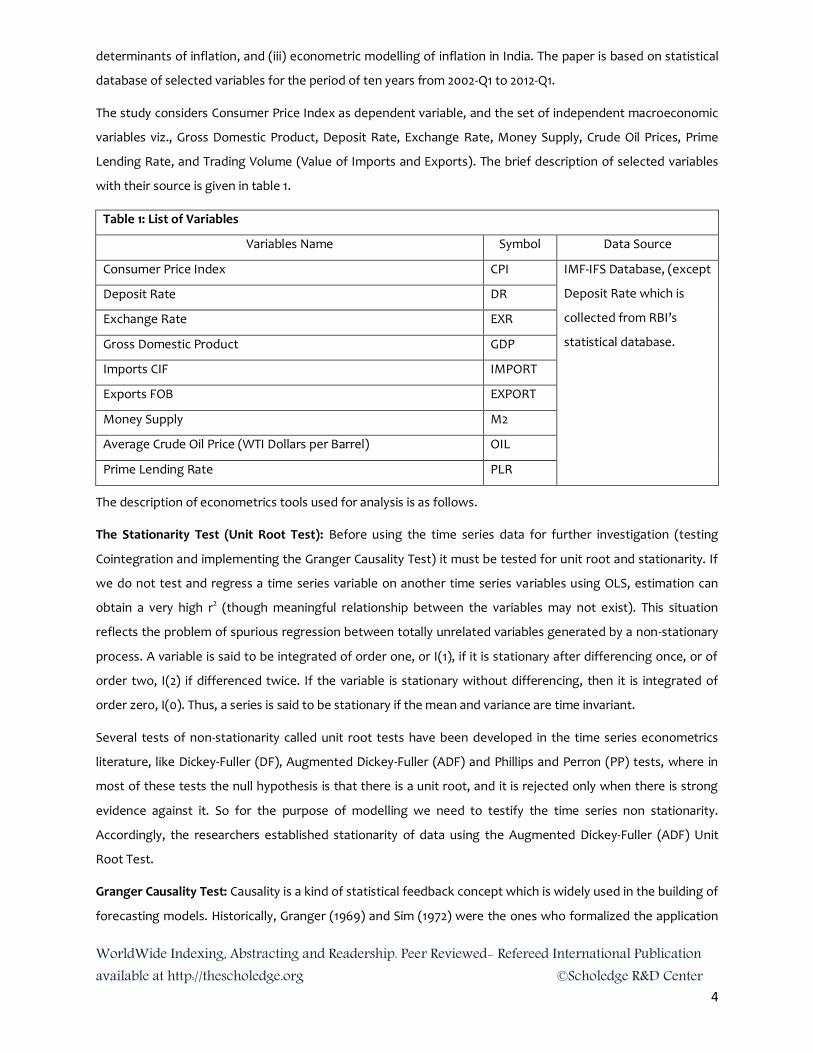
The study considers Consumer Price Index as dependent variable, and the set of independent macroeconomic

variables viz., Gross Domestic Product, Deposit Rate, Exchange Rate, Money Supply, Crude Oil Prices, Prime

Lending Rate, and Trading Volume (Value of Imports and Exports). The brief description of selected variables

with their source is given in table 1.

Table 1: List of Variables

Variables Name Symbol Data Source

Consumer Price Index CPI IMF-IFS Database, (except

Deposit Rate which is

collected from RBI’s

statistical database.

Deposit Rate DR

Exchange Rate EXR

Gross Domestic Product GDP

Imports CIF IMPORT

Exports FOB EXPORT

Money Supply M2

Average Crude Oil Price (WTI Dollars per Barrel) OIL

Prime Lending Rate PLR

The description of econometrics tools used for analysis is as follows.

The Stationarity Test (Unit Root Test): Before using the time series data for further investigation (testing

Cointegration and implementing the Granger Causality Test) it must be tested for unit root and stationarity. If

we do not test and regress a time series variable on another time series variables using OLS, estimation can

obtain a very high r2 (though meaningful relationship between the variables may not exist). This situation

reflects the problem of spurious regression between totally unrelated variables generated by a non-stationary

process. A variable is said to be integrated of order one, or I(1), if it is stationary after differencing once, or of

order two, I(2) if differenced twice. If the variable is stationary without differencing, then it is integrated of

order zero, I(0). Thus, a series is said to be stationary if the mean and variance are time invariant.

Several tests of non-stationarity called unit root tests have been developed in the time series econometrics

literature, like Dickey-Fuller (DF), Augmented Dickey-Fuller (ADF) and Phillips and Perron (PP) tests, where in

most of these tests the null hypothesis is that there is a unit root, and it is rejected only when there is strong

evidence against it. So for the purpose of modelling we need to testify the time series non stationarity.

Accordingly, the researchers established stationarity of data using the Augmented Dickey-Fuller (ADF) Unit

Root Test.

Granger Causality Test: Causality is a kind of statistical feedback concept which is widely used in the building of

forecasting models. Historically, Granger (1969) and Sim (1972) were the ones who formalized the application


5

of causality in economics. Granger causality test is a technique for determining whether one time series is

significant in forecasting another (Granger, 1969). The standard Granger causality test (Granger, 1988) seeks to

determine whether past values of a variable helps to predict changes in another variable. The definition states

that in the conditional distribution, lagged values of Yt add no information to explanation of movements of Xt

beyond that provided by lagged values of Xt itself (Green, 2003). We should take note of the fact that the

Granger causality technique measures the information given by one variable in explaining the latest value of

another variable. In addition, it also says that variable Y is Granger caused by variable X if variable X assists in

predicting the value of variable Y. If this is the case, it means that the lagged values of variable X are statistically

significant in explaining variable Y. The null hypothesis (H0) that we test in this case is that the X variable does

not Granger cause variable Y, and variable Y does not Granger cause variable X. In nutshell, one variable (Xt) is

said to granger cause another variable (Yt) if the lagged values of Xt can predict Yt and vice-versa. The spirit of

Engle and Granger (1987) lies in the idea that if the two variables are integrated as order one, I(1), and both

residuals are I(0), this indicates that the two variables are co integrated. The following model has been

estimated in order to determine the direction of causality.

Let y and x be stationary time series. To test the null hypothesis that x does not Granger cause y, one first finds

the proper lagged values of y to include in a univariate auto regression of y:

Next, the auto regression is augmented by including lagged values of x:

One retains in this regression all lagged values of x that are individually significant according to their t-statistics,

provided that collectively they add explanatory power to the regression according to an F-test (whose null

hypothesis is no explanatory power jointly added by the x's). In the notation of the above augmented

regression, p is the shortest, and q is the longest lag length for which the lagged value of x is significant.

The null hypothesis that x does not Granger-cause y is not rejected if and only if no lagged values of x are

retained in the regression. Granger causality is not necessarily true causality. If both X and Y is driven by a

common third process with different lags, one might still accept the alternative hypothesis of Granger

causality. Yet, manipulation of one of the variables would not change the other. Indeed, the Granger test is

designed to handle pairs of variables, and may produce misleading results when the true relationship involves

three or more variables. A similar test involving more variables can be applied with vector auto regression.

ANALYSIS AND EMPIRICAL RESULTS

TRENDS OF INFLATION: Following figure reflects the changes in inflation in India from the year 2002 Q1 to

2012 Q1.

http://en.wikipedia.org/wiki/Autoregression

http://en.wikipedia.org/wiki/Alternative_hypothesis

http://en.wikipedia.org/wiki/Vector_autoregression


6

Figure 1: Inflation in India: (Consumer Prices Index % Change)

The above graph indicates that the inflation rate in the first quarter of 2001 was 5.10% which decreased up to

quarter two of 2004 (except in 2003 quarter two) and after that severe fluctuations have been seen up to

quarter four of 2009. In 2010 quarter one, inflation rate was at its highest peak of 15.32% and then decreased

continuously up to quarter one of 2012.

BASIC DESCRIPTIVES: Basic descriptives of selected dependent and independent variables presented in (table-

2) indicates that out of all variables only PLR has negative growth rate during the period of study. The value of

standard deviation is very high in case of M2 which indicates very high degree dispersion in data. When we see

the values of skewness, the variables that have positively skewed distribution are DR, EXR and M2, while

negatively skewed distribution is observed in case of remaining variables.

A peaked curve is called leptokurtic, if kurtosis value is greater than 3, Mesokurtic, if kurtosis value is equals to

3, and Platykurtic, if the value of kurtosis is lesser than 3. The values of kurtosis indicates that EXPORT is the

only variable which is platykurtic, while the distribution of variables CPI, DR, EXR, GDP, IMPORT, M2, PLR and

OIL is leptokurtic.

Jarque Bera (JB) test for normality states that the distribution is normal if JB probability is more than 0.05,

otherwise the distribution is considered non-normal. Among the variables under consideration DR, IMPORT,

M2, PLR, and OIL have the non-normal distribution, while CPI, EXR, GDP and EXPORT are normally distributed.

CORRELATIONS: The correlation matrix of selected variables in (table-3) indicates that CPI has negative low

degree correlation with M2, OIL and DR while with other variables has low degree positive correlation and only

PLR is the variable with which it has moderate degree positive correlation.


7

RESULTS OF UNIT ROOT TEST: Before applying causality analysis on the selected variables, it is must to apply a

formal test to confirm whether time series is stationary or not. For this purpose researchers applied

Augmented Dickey Fuller (ADF) test of unit root. The lag length based on the Akaike Information Criterion

(AIC) selected is four. In ADF test, the null hypothesis is that a variable contains a unit root/ are generated by a

non-stationary process, and alternative hypothesis is that the variables are generated by a stationary process/

does not contains unit root. The results of ADF test contained in table 4 show that ‘t’ value of all the variables is

less than critical value. It rejects the null hypotheses at 1 percent level of significance. Hence, it can be said that

all the variables are stationary at level except, CPI which has been made stationary after differencing once.

Thus, researchers made all variables stationary after taking first differences with lag order four (selected on

basis of Akaike Information Criteria).

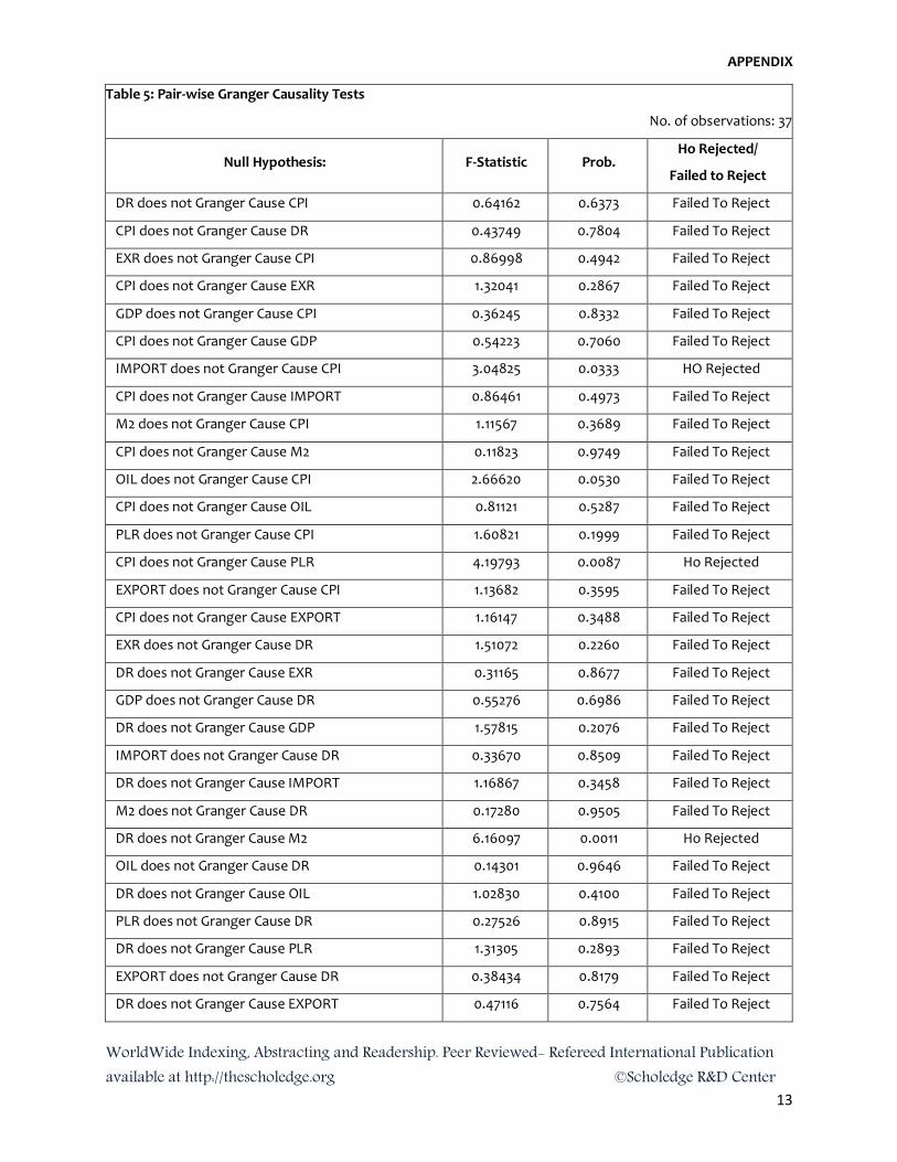
RESULTS OF GRANGER CAUSALITY TEST: The results of causality analysis reported in table 5 (see appendix)

indicate that there exists bidirectional causality between EXPORT and EXR, unidirectional causality between

CPI and IMPORT, CPI and PLR, M2 and DR, IMPORT and EXR, OIL and EXR, M2 and IMPORT, OIL and IMPORT,

EXPORT and IMPORT, OIL and M2, and EXPORT and OIL at 5 percent level of significance. There exists no

causality among remaining variables.


8

Table 2: Descriptive Statistics No. of Observations: 41

CPI DR EXR GDP IMPORT M2 OIL PLR EXPORT

Mean 0.050419 1.993894 0.220222 7.704634 6.434824 5.107312 4.891005 -0.028780 5.582195

Median -0.027850 0.000000 -0.357063 7.770000 4.779797 4.493310 7.915228 0.000000 7.300000

Maximum 2.880400 73.07692 9.403623 10.66000 37.94399 82.16756 38.51173 9.320000 24.65000

Minimum -3.354000 -29.24528 -6.514509 2.310000 -26.02865 -45.97093 -50.57462 -33.33000 -17.96000

Std. Dev. 1.148350 15.64637 3.928849 1.855790 11.00897 16.87482 14.99225 6.423656 9.709562

Skewness -0.146100 2.207755 0.720696 -0.443936 -0.260997 1.727259 -1.197214 -3.263028 -0.336989

Kurtosis 3.868410 11.73688 3.256961 3.143136 5.063734 13.45983 6.426419 18.97672 2.666061

Jarque-Bera 1.434176 163.7093 3.662054 1.381707 7.741271 207.2920 29.85079 508.8185 0.966510

Probability 0.488172 0.000000 0.160249 0.501148 0.020845 0.000000 0.000000 0.000000 0.616772

Table 3: Correlations No. of Observations: 41

CPI DR EXR GDP IMPORT M2 OIL PLR EXPORT

CPI 1.000000 -0.078949 0.123434 0.165080 0.125257 -0.151435 -0.221118 0.364416 0.122834

DR -0.078949 1.000000 0.006381 0.179771 0.046373 0.073219 -0.029340 0.108390 0.155385

EXR 0.123434 0.006381 1.000000 -0.337535 -0.153273 -0.053175 -0.234526 0.190861 0.005732

GDP 0.165080 0.179771 -0.337535 1.000000 0.057451 -0.063941 0.110770 -0.018520 -0.022236

IMPORT 0.125257 0.046373 -0.153273 0.057451 1.000000 -0.026827 -0.206503 0.190160 0.332053

M2 -0.151435 0.073219 -0.053175 -0.063941 -0.026827 1.000000 0.002629 -0.022135 0.233241

OIL -0.221118 -0.029340 -0.234526 0.110770 -0.206503 0.002629 1.000000 -0.238348 0.123434

PLR 0.364416 0.108390 0.190861 -0.018520 0.190160 -0.022135 -0.238348 1.000000 0.112143

EXPORT 0.122834 0.155385 0.005732 -0.022236 0.332053 0.233241 0.123434 0.112143 1.000000

5% Critical value (two-tailed) = 0.3120

VH = Very High (r ≥ 0.75); H = High (0.75 > R ≥ 0.50); M = Moderate (0.50 > R ≥ 0.25); L = Low (r < 0.25); 0 = No Correlation (r = 0)


9

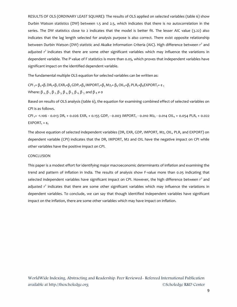
RESULTS OF OLS (ORDINARY LEAST SQUARE): The results of OLS applied on selected variables (table 6) show

Durbin Watson statistics (DW) between 1.5 and 2.5, which indicates that there is no autocorrelation in the

series. The DW statistics close to 2 indicates that the model is better fit. The lesser AIC value (3.22) also

indicates that the lag length selected for analysis purpose is also correct. There exist opposite relationship

between Durbin Watson (DW) statistic and Akaike Information Criteria (AIC). High difference between r2 and

adjusted r2 indicates that there are some other significant variables which may influence the variations in

dependent variable. The P value of F statistics is more than 0.05, which proves that independent variables have

significant impact on the identified dependent variable.

The fundamental multiple OLS equation for selected variables can be written as:

CPI t= βo+β1 DRt+β2 EXRt+β3 GDPt+β4 IMPORTt+β5 M2t+ β6 OILt+β7 PLRt+β8EXPORTt+ ε t

Where: β o, β 1, β 2, β 3, β 4, β 5, β 6, β 7, and β 8 ≠ 0

Based on results of OLS analysis (table 6), the equation for examining combined effect of selected variables on

CPI is as follows.

CPI t= -1.106 - 0.013 DRt + 0.026 EXRt + 0.155 GDPt - 0.003 IMPORTt - 0.010 M2t - 0.014 OILt + 0.054 PLRt + 0.022

EXPORTt + εt

The above equation of selected independent variables (DR, EXR, GDP, IMPORT, M2, OIL, PLR, and EXPORT) on

dependent variable (CPI) indicates that the DR, IMPORT, M2 and OIL have the negative impact on CPI while

other variables have the positive impact on CPI.

CONCLUSION

This paper is a modest effort for identifying major macroeconomic determinants of inflation and examining the

trend and pattern of inflation in India. The results of analysis show F-value more than 0.05 indicating that

selected independent variables have significant impact on CPI. However, the high difference between r2 and

adjusted r2 indicates that there are some other significant variables which may influence the variations in

dependent variables. To conclude, we can say that though identified independent variables have significant

impact on the inflation, there are some other variables which may have impact on inflation.


10

Table 4: Results of Unit Root Test

No. of Observations 41

S. No. Variables ADF t-Value (Level) Prob. Value Order of Integration Remark

1 DCPI* -4.873001 0.0003 I(1) Stationary

2 DR -7.222632 0.0000 I(0) Stationary

3 EXR -4.847617 0.0003 I(0) Stationary

4 GDP -3.051838 0.0386 I(0) Stationary

5 IMPORT -6.268033 0.0000 I(0) Stationary

6 M2 -9.522015 0.0000 I(0) Stationary

7 OIL -5.707853 0.0000 I(0) Stationary

8 PLR -6.334555 0.0000 I(0) Stationary

9 EXPORT -7.475092 0.0000 I(0) Stationary

Note: 1%, 5 % and 10% critical values are -3.505, -2.889 and -2.579 respectively. * D denotes differencing of variable.

Table 6: Results of OLS

Dependent Variable: CPI Number of observations: 41

Variables Coefficient Std. Error t-Stat. (P-Value) F-Ratio

(P-Value) SE Est.

R2&

Adj. R2 AIC SWC DW

C -1.107 0.826 -1.340 (0.190) 1.435

(0.22)

1.101 0.264

0.080

3.222 3.598 1.659

DR -0.013 0.0116 -1.145 (0.261)

EXR 0.027 0.051 0.532 (0.598)

GDP 0.156 0.1021 1.519 (0.139)

IMPORT -0.003 0.0181 -0.183 (0.856)

M2 -0.011 0.011 -0.979 (0.335)

OIL -0.015 0.013 -1.118 (0.272)

PLR 0.055 0.029 1.897 (0.067)

EXPORT 0.023 0.021 1.098 (0.280)


11

REFERENCES

Abidemi, OI and Malik, SAA. 2010. “Analysis of Inflation and its Determinant in Nigeria”, Pakistan

Journal of Social Sciences, 7(2).

Acharya Shankar. 2012. “India: After the Global Crisis”, Orient BlackSwan Private Limited, Hyderabad.

Andersson M, Masuch K and Schiffbauer M. 2009. “Determinants of Inflation and Price Level Differentials

across the Euro Area Countries”, European Central Bank, Working Paper No. 1129.

Batura, N. 2008. “Understanding Recent Trends in Inflation”, Economic & Political Weekly, Vol. XLIII(24),

June 14-20.

Bishnoi, TR and TP Koirala. 2006. “Stability and Robustness of Inflation Model”, Journal of Quantitative

Economics, Volume 4(2), June.

Cheng Hoon Lim and Laura Papi. 1997. “An Econometric Analysis of the Determinants of Inflation in Turkey”,

IMF Working Paper No. 97/170.

Dua Pami and Upasna Gaur. 2009. “Determination of Inflation in an Open Economy Phillips Curve

Framework: The Case of Developed and Developing Asian Countries”, Working Paper No. 178, Centre for

Development Economics, Delhi School of Economics, Delhi, April.

Experts and Scholars from BRICS Countries. 2012. “The BRICS Report”, First Edition, Oxford University

Press, New Delhi.

Gary G Moser. 1995. “The Main Determinants of Inflation in Nigeria”, IMF Staff Papers, Vol. 42(2).

Government of India. 2012. Economic Survey, Ministry of Finance, New Delhi.

Greenidge Kevin and Dianna DaCosta. 2009. “Determinants of Inflation in Selected Caribbean Countries”,

Business, Finance & Economics in Emerging Economies, Vol. 4(2).

Ilker Domaç. 1998. “The Main Determinants of inflation in Albania”, World Bank Policy Research

Working Paper No. 1930.

Jan Gottschalk, Kadima Kalonji, and Ken Miyajima. 2008. “Analyzing Determinants of Inflation When There

Are Data Limitations: The Case of Sierra Leone”, IMF Working Paper.

John, RM. 2003. “Inflation in India: An Analysis Using Post Liberalized Data”, IGIDR Working Paper.

Kandil M and Morsy H. 2009. “Determinants of Inflation in GCC”, IMF Working Paper No. 09/82.

Kishor N Kundan. 2009. “Modeling Inflation in India: The Role of Money”, MPRA Paper No. 16098.

Kuijs, L. 1998. “Determinants of Inflation, Exchange Rate and Output in Nigeria”. IMF working Paper

No. 160.

Lakshmi R. 2002. “Dynamics of Inflation in India: A P-Star Approach”, Applied Economics, 34(1).


12

Lim, CH, and Papi, L. 1997. “An Econometric Analysis of the Determinants of Inflation in Turkey”, IMF Working

Paper No. 170.

Liu, O, and Adedeji, OS. 2000. “Determinants of Inflation in the Islamic Republic of Iran: A Macroeconomic

Analysis”, IMF Working Paper No. 127.

Maddala GS. 2001. “Introduction to Econometrics”, Third Edition, John Wiley and Sons, Singapore.

Mallik G and Chowdhury A. 2001. “Inflation and Economic Growth: Evidence from South Asian Countries”,

Asian Pacific Development Journal, Vol. 8(1).

Srinivasan, NV, Mahambare, and M Ramachandran. 2006. “Modelling Inflation in India: A Critique of the

Structural Approach”, Journal of Quantitative Economics, Vol. 4(2), June.

Wang X. 2010. “The Relationship between Stock Market Volatility and Macroeconomic Volatility: Evidence

from China”, International Research Journal of Finance, 7396 African Journal of Business Management

Economics, 49.


13

APPENDIX

Table 5: Pair-wise Granger Causality Tests

No. of observations: 37

Null Hypothesis: F-Statistic Prob. Ho Rejected/

Failed to Reject

DR does not Granger Cause CPI 0.64162 0.6373 Failed To Reject

CPI does not Granger Cause DR 0.43749 0.7804 Failed To Reject

EXR does not Granger Cause CPI 0.86998 0.4942 Failed To Reject

CPI does not Granger Cause EXR 1.32041 0.2867 Failed To Reject

GDP does not Granger Cause CPI 0.36245 0.8332 Failed To Reject

CPI does not Granger Cause GDP 0.54223 0.7060 Failed To Reject

IMPORT does not Granger Cause CPI 3.04825 0.0333 HO Rejected

CPI does not Granger Cause IMPORT 0.86461 0.4973 Failed To Reject

M2 does not Granger Cause CPI 1.11567 0.3689 Failed To Reject

CPI does not Granger Cause M2 0.11823 0.9749 Failed To Reject

OIL does not Granger Cause CPI 2.66620 0.0530 Failed To Reject

CPI does not Granger Cause OIL 0.81121 0.5287 Failed To Reject

PLR does not Granger Cause CPI 1.60821 0.1999 Failed To Reject

CPI does not Granger Cause PLR 4.19793 0.0087 Ho Rejected

EXPORT does not Granger Cause CPI 1.13682 0.3595 Failed To Reject

CPI does not Granger Cause EXPORT 1.16147 0.3488 Failed To Reject

EXR does not Granger Cause DR 1.51072 0.2260 Failed To Reject

DR does not Granger Cause EXR 0.31165 0.8677 Failed To Reject

GDP does not Granger Cause DR 0.55276 0.6986 Failed To Reject

DR does not Granger Cause GDP 1.57815 0.2076 Failed To Reject

IMPORT does not Granger Cause DR 0.33670 0.8509 Failed To Reject

DR does not Granger Cause IMPORT 1.16867 0.3458 Failed To Reject

M2 does not Granger Cause DR 0.17280 0.9505 Failed To Reject

DR does not Granger Cause M2 6.16097 0.0011 Ho Rejected

OIL does not Granger Cause DR 0.14301 0.9646 Failed To Reject

DR does not Granger Cause OIL 1.02830 0.4100 Failed To Reject

PLR does not Granger Cause DR 0.27526 0.8915 Failed To Reject

DR does not Granger Cause PLR 1.31305 0.2893 Failed To Reject

EXPORT does not Granger Cause DR 0.38434 0.8179 Failed To Reject

DR does not Granger Cause EXPORT 0.47116 0.7564 Failed To Reject


14

GDP does not Granger Cause EXR 0.40364 0.8044 Failed To Reject

EXR does not Granger Cause GDP 0.37721 0.8229 Failed To Reject

IMPORT does not Granger Cause EXR 1.24900 0.3132 Failed To Reject

EXR does not Granger Cause IMPORT 3.00471 0.0351 HO Rejected

M2 does not Granger Cause EXR 1.02970 0.4093 Failed To Reject

EXR does not Granger Cause M2 0.82428 0.5208 Failed To Reject

OIL does not Granger Cause EXR 0.64521 0.6349 Failed To Reject

EXR does not Granger Cause OIL 2.88304 0.0407 HO Rejected

PLR does not Granger Cause EXR 0.34404 0.8459 Failed To Reject

EXR does not Granger Cause PLR 0.35436 0.8388 Failed To Reject

EXPORT does not Granger Cause EXR 2.95941 0.0370 HO Rejected

EXR does not Granger Cause EXPORT 4.59309 0.0056 HO Rejected

IMPORT does not Granger Cause GDP 0.82077 0.5229 Failed To Reject

GDP does not Granger Cause IMPORT 1.36593 0.2709 Failed To Reject

M2 does not Granger Cause GDP 0.91030 0.4715 Failed To Reject

GDP does not Granger Cause M2 0.30640 0.8712 Failed To Reject

OIL does not Granger Cause GDP 0.37156 0.8269 Failed To Reject

GDP does not Granger Cause OIL 0.45802 0.7658 Failed To Reject

PLR does not Granger Cause GDP 0.16543 0.9541 Failed To Reject

GDP does not Granger Cause PLR 0.94106 0.4548 Failed To Reject

EXPORT does not Granger Cause GDP 0.78496 0.5446 Failed To Reject

GDP does not Granger Cause EXPORT 0.31321 0.8667 Failed To Reject

M2 does not Granger Cause IMPORT 2.99049 0.0357 HO Rejected

IMPORT does not Granger Cause M2 0.40110 0.8062 Failed To Reject

OIL does not Granger Cause IMPORT 5.55288 0.0020 Ho Rejected

IMPORT does not Granger Cause OIL 2.04360 0.1154 Failed To Reject

PLR does not Granger Cause IMPORT 0.17404 0.9499 Failed To Reject

IMPORT does not Granger Cause PLR 0.38982 0.8141 Failed To Reject

EXPORT does not Granger Cause IMPORT 4.39980 0.0069 Ho Rejected

IMPORT does not Granger Cause EXPORT 0.30950 0.8692 Failed To Reject

OIL does not Granger Cause M2 1.52050 0.2232 Failed To Reject

M2 does not Granger Cause OIL 6.32416 0.0009 Ho Rejected

PLR does not Granger Cause M2 0.65737 0.6267 Failed To Reject

M2 does not Granger Cause PLR 0.47279 0.7553 Failed To Reject

EXPORT does not Granger Cause M2 0.27419 0.8921 Failed To Reject


15

M2 does not Granger Cause EXPORT 1.45312 0.2429 Failed To Reject

PLR does not Granger Cause OIL 0.32410 0.8594 Failed To Reject

OIL does not Granger Cause PLR 0.22597 0.9216 Failed To Reject

EXPORT does not Granger Cause OIL 1.75826 0.1654 Failed To Reject

OIL does not Granger Cause EXPORT 3.87619 0.0125 HO Rejected

EXPORT does not Granger Cause PLR 0.10946 0.9782 Failed To Reject

PLR does not Granger Cause EXPORT 0.82587 0.5199 Failed To Reject

Note: (i) Significant at 5% confidence level. (ii) AIC is used to determine appropriate lag lengths.

determinants of inflation in india: an econometric analysis

Economy & Finance