DETERMINANTS OF FOOD PRICE INFLATION IN

PAKISTAN

MUHAMMAD ABDULLAH

National College of Business Administration and Economics, Lahore

PROF. DR. RUKHSANA KALIM

University of Management and Technology, Lahore

This study focuses on the identification of main determinants of food price

inflation in Pakistan. Using the data from 1972 to 2008, Johansen’s co-

integration technique is utilized to find out the long run relationships among

food price inflation and its determinants like inflation expectations, money

supply, per capita GDP, support prices, food imports and food exports.

Empirical findings prove the long run relationships among food price

inflation and its determinants. All the determinants affect food price

inflation positively and significantly except money supply which is

insignificant with correct positive sign. Vector Error Correction Model

(VECM) has been used for the analysis of short run dynamics. In the short

run, only inflation expectations, support prices and food exports affect the

food price inflation. The results reveal that both demand and supply side

factors are the determinants food price inflation in Pakistan. However, our

study supports the structuralist point of view of inflation as money supply

shows insignificant results.

1. INTRODUCTION

In the recent years, food price inflation has risen very sharply at global level.

According to Commodity Research Bureau (2009), the overall and food

inflation rates at global level stand at 16.5 and 30.2 percent respectively by

November 06, 2007. This high food inflation persists in most of the

countries in the world. Reduced level of poverty, increase in per capita

income and urbanization are main reasons of sharp increase in demand and

prices of some basic food items. When income increases, dietary habits also

change, people expand their expenditures to have more food and meat. For

example, in China per capita consumption of meat at 20 Kg in 1985

increased to 50 Kg in 2007(Abhayaratne and Kasturi, 2008). There is 17 per

cent boost in grain consumption from 2000 to 2005 among the oil producing

and exporting countries (OPEC) because of their huge export earnings

(World Bank, 2007). Demand for bio fuels in rich countries is also an

important contributor towards higher prices of some basic food items. There

seems a link between food and energy prices as since 2000, prices of oil and

wheat have become triple and prices of corn and rice are double now (IFPRI,

2007).

Food inflation has increased the living cost of households

especially in developing countries like Pakistan. Because of higher food

inflation, households have to make reductions in some areas of food

consumption leading to malnutrition. Malnutrition results in productivity

losses of up to 10 percent of lifetime earnings and GDP losses of 2-3 percent

in the worst affected countries (Alderman, 2005). High inflation erodes the

benefits of growth and leaves the poor worse off (Esterly and Ficsher, 2001).

It hurts the poor more, since more than half of the budget of low wage

earners goes toward food. It redistributes income from fixed income groups

to the owners of assets and businessmen and increases the gap between rich

and poor (Khan et al, 2007).

There are many factors contributing towards food inflation in

Pakistan. Our domestic consumption is increasing because of growth in

population and per capita income. There is lack of cold storages and proper

marketing of perishable goods, therefore, if there is increase in demand or

shortage in supply, prices will increase. A variety of agricultural and non-

agricultural commodities is traded illegally at Pak-Afghan and Pak-Iran

borders which creates substantial monetary loss to the Government of

Pakistan in terms of public revenues which might be collected in the form of

duties and taxes (Sharif et al. 2000).

In Pakistan, food inflation remained 9.9 % on average during the

study period (1972-2008) and below 10 % during 1997-08 to 2003-04. It

started to accelerate after 2003-04 and increased up to 12.5% in 2004-05. It

was 17.5 % and 26.6 % in 2007-08 and 2008-09 respectively. This sudden

rise in food inflation was because of shortages of wheat, increase in the

support price of wheat, increase in prices of some food items such as rice,

edible oil, meat, pulses, tea, milk, fresh vegetables and fruit and a rise in

international prices of food items along with the oil prices(Government of

Pakistan, 2007, 2009). This high food inflation is a matter of great concern

for policy makers. This study tries to find out the main determinants of food

price inflation in Pakistan.

The rest of study is designed as follows: The relevant literature on

food price inflation is discussed in section 2. Section 3 is devoted to the

theoretical framework, methodology and econometric techniques used in this

study. Empirical results are discussed in section 4. Section five concludes

the major findings of the study and suggests some policy implications.

2. LITERATURE REVIEW

The economic literature reveals that demand-side factors and supply-

side factors are two major sources of inflation. These factors are discussed

under two schools of thoughts, the monetarist and the structuralist.

The monetarist model has its theoretical foundations on the quantity

theory of money which is part of the classical economic theory. It was

presented by Friedman (1968, 1970 and 1971). ‘Inflation is always and

everywhere a monetary phenomenon’ is the famous statement of this theory.

Schwartz (1973) tested it empirically. Monetarists are in the view that

increase in the money supply results in proportionate increases in the prices,

assuming economic agents rational and output and real money balances

constant.

The structuralist models of inflation emerged in the 1950s. These

were supported by Streeten (1962), Olivera (1964), Baumol (1967) and

Maynard and Rijckeghem (1976). According to these models, supply-side

factors like food prices, administered prices, wages and import prices are the

determinants of inflation.

Bhattacharia and Lodh (1990) supported the superiority of strcturalists

model in the case of India. Balkrishnan (1992) applied structuralist approach

through error correction specification for modeling inflation in India. He

concluded that labour and raw material costs were significant determinants

of inflation in industrial sector. In agriculture sector, prices of food grains

were determined by per capita output, per capita income in agriculture sector

and government procurement of food grains. Balkrishnan (1994) found that

structulists model was better than monetarist’s model.

Khan and Qasim (1996) studied general inflation and food price

inflation separately. They found that inflation is co integrated with money

supply (M2), import price and real GDP. Money supply (M2) and import

prices affect inflation positively while GDP has negative relation with

inflation. According to their findings, food inflation has also long run

relationship with money supply, value added in agriculture and wheat

support prices. Money supply and wheat support prices showed positive

relation with food price inflation and agriculture output was negatively

cointegrated with food price inflation.

Hasan et al. (2005) estimated the disaggregated inflation model with

respect to different sectors (of Wholesale Price Index) according to their

weights in aggregated inflation model. They studied three elements of

Wholesale Price Index (WPI) out five. These were food, raw material and

manufacturing assuming that remaining two sectors energy and building

material were exogenously determined. They concluded that supply shocks

(production of agricultural goods) have negative impact on food price

inflation. Impacts of support prices of wheat and expectations about future

inflation were positive and highly significant on food price inflation. Money

supply or monetary policy showed an insignificant impact on agriculture

food prices while its impact on raw material and manufacturing was

significant.

Khan and Schimimelpfenning (2006) found that monetary factors

determined the inflation in Pakistan. Broad money growth and private sector

credit growth were the key variables of inflation. They included money

supply and credit to private sector as standard monetary variables, exchange

rate and wheat support prices as supply side factors. Support prices

influenced inflation only in short run.

Tweeten (1980) argued that the monetary shocks had little effect on

the agricultural prices. Devadoss and Meyers (1987) were of the view that

agricultural prices had faster response, as compared to the prices of

manufacturing products, to a change in money supply in the U.S.A.

Saghaian et al. (2002) claimed money neutrality did not hold in the

determination of agricultural prices in U.S.A. Xuehua et al. (2004) and

Bruno et al. (2005) rejected the non neutrality of money supply in the

determination of food prices.

Lorie and Khan (2006) concluded that there was only a weak evidence

of the existence of long run co integration between domestic prices,

international prices and support prices for key agricultural goods in Pakistan.

Only in the case of wheat, the evidence was strong. The elasticity of

domestic prices to a change in the exchange rate was close to unity for all

commodities.

The increase in demand for globally traded food crops is the basic

reason of increase in food prices. Furthermore, increasing interest of global

investors in hording commodity for future contracts has a contribution to the

rise in food prices recently (Johnson, 2008),

According to the Asian Development Bank Report (2008), there were

different structural and cyclical factors determining the food prices in

developing Asian countries. Production growth had fallen below the

consumption growth for several years. There was 43% decline in rice and

wheat stocks during 2000 and 2007. International rice markets were

extremely thin because of large number of consuming countries and small

number of producing countries (USDA, 2008).

Loening et al (2009) studied inflation dynamics and food prices in

Ethopia. They found that international food commodity prices and producer

prices determine the domestic food and non-food prices in Ethopia. Inflation

expectations (inertia) affected food price inflation more as compared to non-

food inflation. In the short and medium run, agriculture supply shocks and

inertia affect the inflation in the country. They found no evidence of direct

impact of excess money supply and world energy price inflation on both

food and non-food inflation.

On the basis of the discussion held above it is evident that researchers

mad an effort to identify the major causes of inflation from one or the other

perspective. In the present paper both the monetarist and structuralist point

of view has been considered together to explore the factors affecting food

inflation in Pakistan.

3. METHODOLOGY AND DATA SOURCES Economic literature on inflation provides some models that

incorporate the demand and supply side factors (Hassan et al., 1995; Khan

and Qasim, 1996; Callen and Chang, 1999; Bokil and Schimmelfennig, 2005

and Khan and Schimmelfennig, 2006). Following Khan and Schimmelfennig

(2006), the stylized hybrid monetarists-structulists model given below is

formulated to capture the effect of certain demand and supply side factors of

food price inflation in Pakistan.

t t-1 t t t t tFPI f (FPI ,M2G ,PGDP ,ASP ,FX ,FM )

(1)

where

t= 1, 2, 3, …., 37. (time period ranging from 1972-2008)

tFPI = Food Price Inflation (CPI food as proxy of Food Price

Inflation) in time t

t 1FPI = One year lag of tFPI (as proxy of inflation expectations)

tM2G = Growth Rate of Money Supply (M2) in time t

tPGDP = Per Capita GDP (in Pak rupees) in time t

tASP = Agriculture Support Price (rupees/40kg of wheat) in time t

tFX = Food Export (as percentage of merchandise export) in time t

tFM = Food Import (as percentage of merchandise imports) in time t.

Equation (1) can be rewritten for estimation purposes as follows:

t 0 1 t-1 2 t 3 t 4 t

5 t 6 t t

FPI FPI M2G PGDP ASP

FX FM (2)

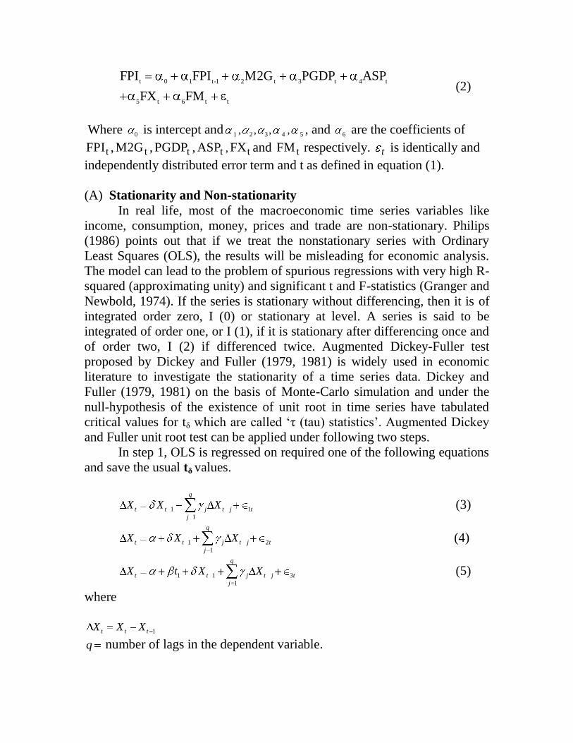
Where 0 is intercept and 1 2 3 4 5, , , , , and 6 are the coefficients of

tFPI , tM2G , tPGDP , tASP , tFX and tFM respectively. t is identically and

independently distributed error term and t as defined in equation (1).

(A) Stationarity and Non-stationarity

In real life, most of the macroeconomic time series variables like

income, consumption, money, prices and trade are non-stationary. Philips

(1986) points out that if we treat the nonstationary series with Ordinary

Least Squares (OLS), the results will be misleading for economic analysis.

The model can lead to the problem of spurious regressions with very high R-

squared (approximating unity) and significant t and F-statistics (Granger and

Newbold, 1974). If the series is stationary without differencing, then it is of

integrated order zero, I (0) or stationary at level. A series is said to be

integrated of order one, or I (1), if it is stationary after differencing once and

of order two, I (2) if differenced twice. Augmented Dickey-Fuller test

proposed by Dickey and Fuller (1979, 1981) is widely used in economic

literature to investigate the stationarity of a time series data. Dickey and

Fuller (1979, 1981) on the basis of Monte-Carlo simulation and under the

null-hypothesis of the existence of unit root in time series have tabulated

critical values for tδ which are called ‘τ (tau) statistics’. Augmented Dickey

and Fuller unit root test can be applied under following two steps.

In step 1, OLS is regressed on required one of the following equations

and save the usual tδ values.

1 1

1

q

t t j t j t

j

X X X (3)

1 2

1

q

t t j t j t

j

X X X (4)

1 1 3

1

q

t t j t j t

j

X t X X (5)

where

1t t tX X X

q number of lags in the dependent variable.

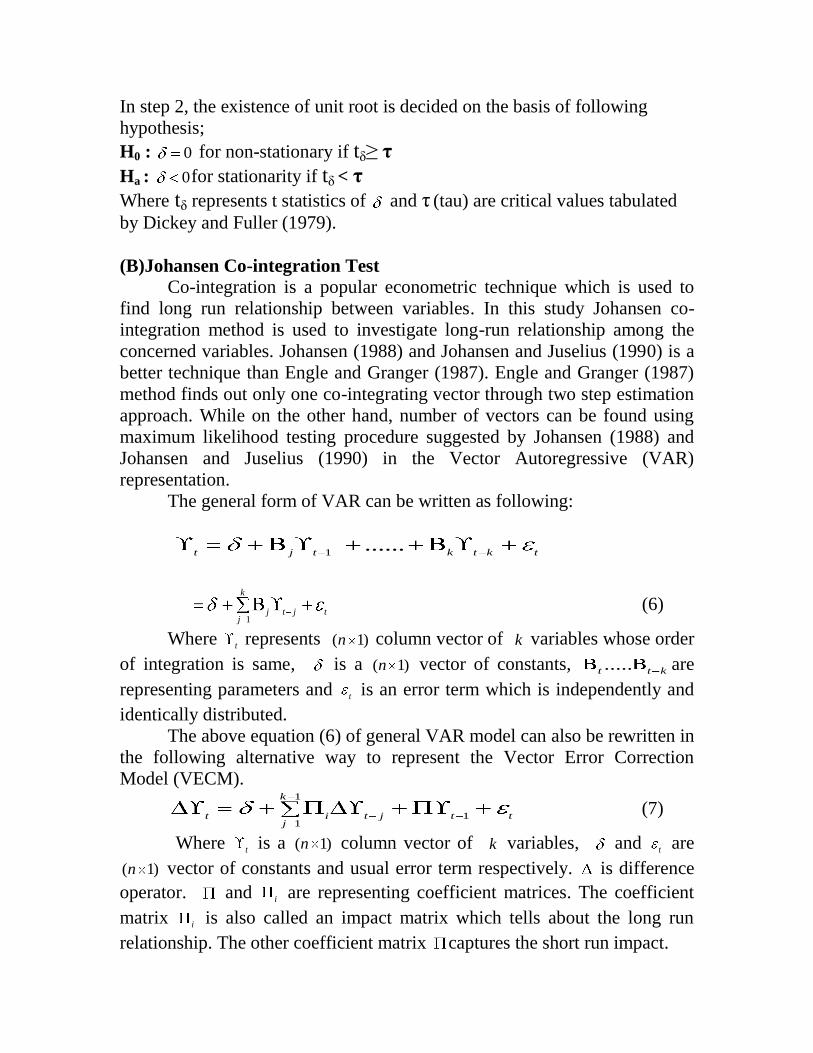
In step 2, the existence of unit root is decided on the basis of following

hypothesis;

H0 : 0 for non-stationary if tδ≥ τ

Ha : 0for stationarity if tδ < τ

Where tδ represents t statistics of and τ (tau) are critical values tabulated

by Dickey and Fuller (1979).

(B)Johansen Co-integration Test

Co-integration is a popular econometric technique which is used to

find long run relationship between variables. In this study Johansen co-

integration method is used to investigate long-run relationship among the

concerned variables. Johansen (1988) and Johansen and Juselius (1990) is a

better technique than Engle and Granger (1987). Engle and Granger (1987)

method finds out only one co-integrating vector through two step estimation

approach. While on the other hand, number of vectors can be found using

maximum likelihood testing procedure suggested by Johansen (1988) and

Johansen and Juselius (1990) in the Vector Autoregressive (VAR)

representation.

The general form of VAR can be written as following:

1......

t j t k t k t

1

k

j t j tj

(6)

Where t represents ( 1)n column vector of k variables whose order

of integration is same, is a ( 1)n vector of constants, .....t t k are

representing parameters and t is an error term which is independently and

identically distributed.

The above equation (6) of general VAR model can also be rewritten in

the following alternative way to represent the Vector Error Correction

Model (VECM). 1

11

k

t i t j t tj

(7)

Where t is a ( 1)n column vector of k variables, and t are

( 1)n vector of constants and usual error term respectively. is difference

operator. and i are representing coefficient matrices. The coefficient

matrix i is also called an impact matrix which tells about the long run

relationship. The other coefficient matrix captures the short run impact.

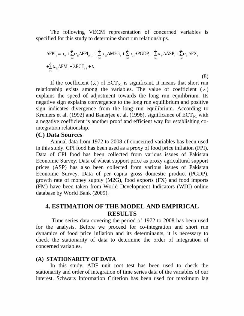
The following VECM representation of concerned variables is

specified for this study to determine short run relationships.

n n n n n

t 0 1j ( t 1) 2 j t 3 j t 4 j t 5 j tj 1 j 1 j 1 j 1 j 1

n

6 j t t 1 tj 1

FPI FPI M2G PGDP ASP FX

FM ECT

(8)

If the coefficient ( ) of ECTt-1 is significant, it means that short run

relationship exists among the variables. The value of coefficient ( )

explains the speed of adjustment towards the long run equilibrium. Its

negative sign explains convergence to the long run equilibrium and positive

sign indicates divergence from the long run equilibrium. According to

Kremers et al. (1992) and Banerjee et al. (1998), significance of ECTt-1 with

a negative coefficient is another proof and efficient way for establishing co-

integration relationship.

(C) Data Sources Annual data from 1972 to 2008 of concerned variables has been used

in this study. CPI food has been used as a proxy of food price inflation (FPI).

Data of CPI food has been collected from various issues of Pakistan

Economic Survey. Data of wheat support price as proxy agricultural support

prices (ASP) has also been collected from various issues of Pakistan

Economic Survey. Data of per capita gross domestic product (PGDP),

growth rate of money supply (M2G), food exports (FX) and food imports

(FM) have been taken from World Development Indicators (WDI) online

database by World Bank (2009).

4. ESTIMATION OF THE MODEL AND EMPIRICAL

RESULTS Time series data covering the period of 1972 to 2008 has been used

for the analysis. Before we proceed for co-integration and short run

dynamics of food price inflation and its determinants, it is necessary to

check the stationarity of data to determine the order of integration of

concerned variables.

(A) STATIONARITY OF DATA

In this study, ADF unit root test has been used to check the

stationarity and order of integration of time series data of the variables of our

interest. Schwarz Information Criterion has been used for maximum lag

selection for applying ADF unit root test. The results of ADF test are

presented in table-1.

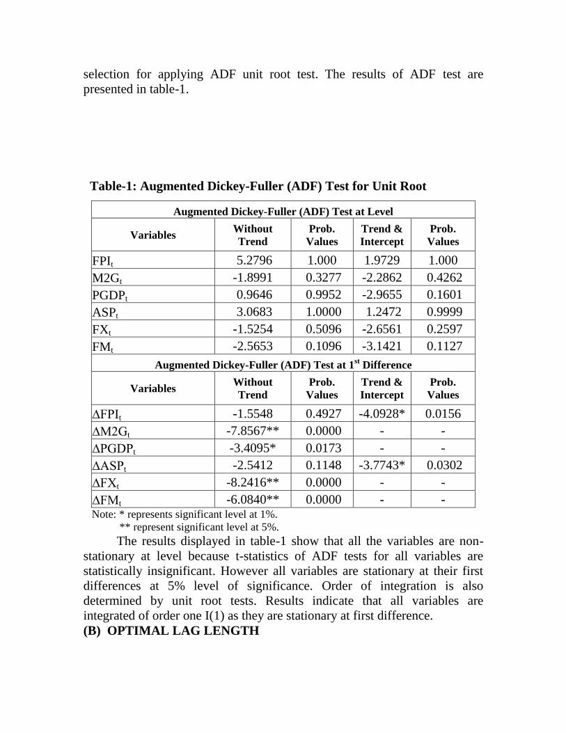
Table-1: Augmented Dickey-Fuller (ADF) Test for Unit Root

Augmented Dickey-Fuller (ADF) Test at Level

Variables Without

Trend

Prob.

Values

Trend &

Intercept

Prob.

Values

FPIt 5.2796 1.000 1.9729 1.000

M2Gt -1.8991 0.3277 -2.2862 0.4262

PGDPt 0.9646 0.9952 -2.9655 0.1601

ASPt 3.0683 1.0000 1.2472 0.9999

FXt -1.5254 0.5096 -2.6561 0.2597

FMt -2.5653 0.1096 -3.1421 0.1127

Augmented Dickey-Fuller (ADF) Test at 1st Difference

Variables Without

Trend

Prob.

Values

Trend &

Intercept

Prob.

Values

∆FPIt -1.5548 0.4927 -4.0928* 0.0156

∆M2Gt -7.8567** 0.0000 - -

∆PGDPt -3.4095* 0.0173 - -

∆ASPt -2.5412 0.1148 -3.7743* 0.0302

∆FXt -8.2416** 0.0000 - -

∆FMt -6.0840** 0.0000 - - Note: * represents significant level at 1%.

** represent significant level at 5%.

The results displayed in table-1 show that all the variables are non-

stationary at level because t-statistics of ADF tests for all variables are

statistically insignificant. However all variables are stationary at their first

differences at 5% level of significance. Order of integration is also

determined by unit root tests. Results indicate that all variables are

integrated of order one I(1) as they are stationary at first difference.

(B) OPTIMAL LAG LENGTH

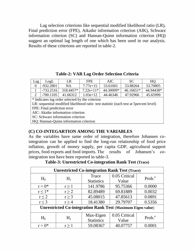
Lag selection criterions like sequential modified likelihood ratio (LR),

Final prediction error (FPE), Aikaike information criterion (AIK), Schwarz

information criterion (SC) and Hannan-Quinn information criterion (HQ)

suggest an optimal lag length of one which has been used in our analysis.

Results of these criterions are reported in table-2.

Table-2: VAR Lag Order Selection Criteria

Lag LogL LR FPE AIC SC HQ

0 -932.2801 NA 7.77e+15 53.61601 53.88264 53.70805

1 -733.2516 318.4457* 7.22e+11* 44.30009* 46.16651* 44.94438*

2 -700.1105 41.66312 1.03e+12 44.46346 47.92966 45.65999

* Indicates lag order selected by the criterion

LR: sequential modified likelihood ratio test statistic (each test at 5percent level)

FPE: Final prediction error

AIC: Akaike information criterion

SC: Schwarz information criterion

HQ: Hannan-Quinn information criterion

(C) CO-INTEGARTION AMONG THE VARIABLES

As the variables have same order of integration, therefore Johansen co-

integration can be applied to find the long-run relationship of food price

inflation, growth of money supply, per capita GDP, agricultural support

prices, food exports and food imports. The results of Johansen’s co-

integration test have been reported in table-3.

Table-3: Unrestricted Co-integration Rank Test (Trace)

Unrestricted Co-integration Rank Test (Trace)

H0 H1 Trace

Statistics

0.05 Critical

Value Prob.

a

r = 0* r ≥ 1 141.9786 95.75366 0.0000

r ≤ 1* r ≥ 2 82.89489 69.81889 0.0032

r ≤ 2 r ≥ 3 45.08015 47.85613 0.0891

r ≤ 3 r ≥ 4 18.41380 29.79707 0.5356

Unrestricted Co-integration Rank Test (Maximum Eigen value)

H0 H1 Max-Eigen

Statistics

0.05 Critical

Value Prob.

a

r = 0* r ≥ 1 59.08367 40.07757 0.0001

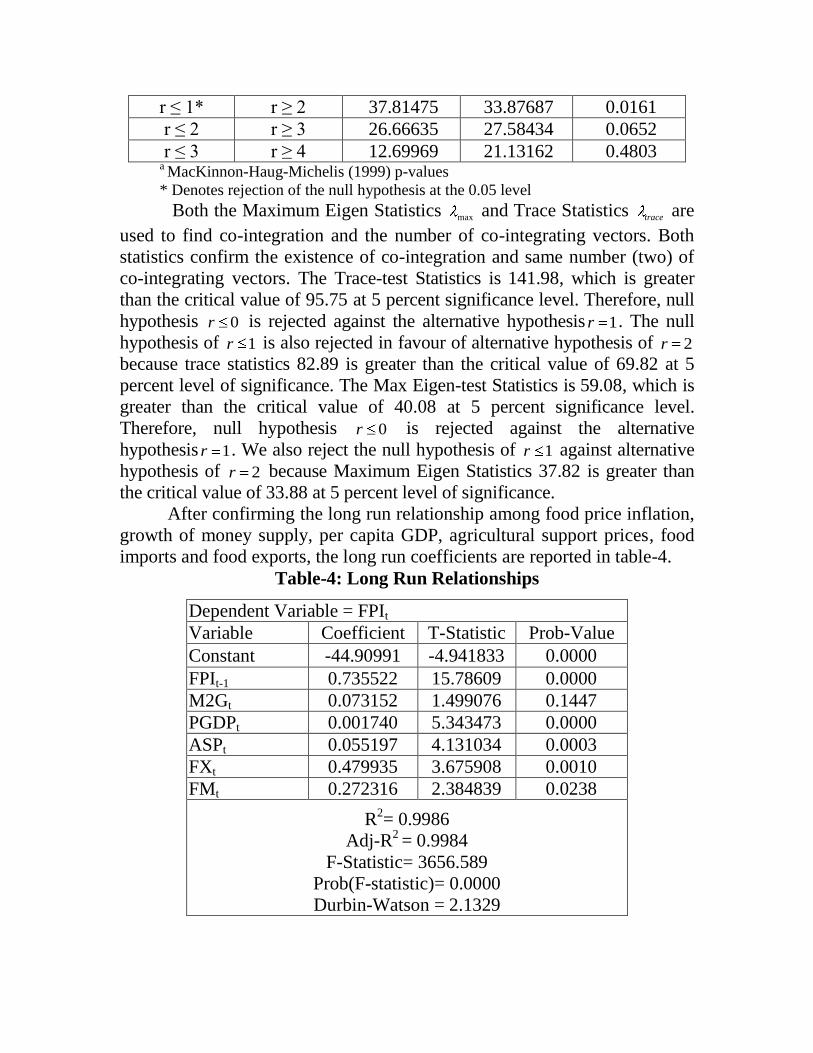
r ≤ 1* r ≥ 2 37.81475 33.87687 0.0161

r ≤ 2 r ≥ 3 26.66635 27.58434 0.0652

r ≤ 3 r ≥ 4 12.69969 21.13162 0.4803

a MacKinnon-Haug-Michelis (1999) p-values

* Denotes rejection of the null hypothesis at the 0.05 level

Both the Maximum Eigen Statistics max and Trace Statistics trace are

used to find co-integration and the number of co-integrating vectors. Both

statistics confirm the existence of co-integration and same number (two) of

co-integrating vectors. The Trace-test Statistics is 141.98, which is greater

than the critical value of 95.75 at 5 percent significance level. Therefore, null

hypothesis 0r is rejected against the alternative hypothesis 1r . The null

hypothesis of 1r is also rejected in favour of alternative hypothesis of 2r

because trace statistics 82.89 is greater than the critical value of 69.82 at 5

percent level of significance. The Max Eigen-test Statistics is 59.08, which is

greater than the critical value of 40.08 at 5 percent significance level.

Therefore, null hypothesis 0r is rejected against the alternative

hypothesis 1r . We also reject the null hypothesis of 1r against alternative

hypothesis of 2r because Maximum Eigen Statistics 37.82 is greater than

the critical value of 33.88 at 5 percent level of significance.

After confirming the long run relationship among food price inflation,

growth of money supply, per capita GDP, agricultural support prices, food

imports and food exports, the long run coefficients are reported in table-4.

Table-4: Long Run Relationships

Dependent Variable = FPIt

Variable Coefficient T-Statistic Prob-Value

Constant -44.90991 -4.941833 0.0000

FPIt-1 0.735522 15.78609 0.0000

M2Gt 0.073152 1.499076 0.1447

PGDPt 0.001740 5.343473 0.0000

ASPt 0.055197 4.131034 0.0003

FXt 0.479935 3.675908 0.0010

FMt 0.272316 2.384839 0.0238

R2= 0.9986

Adj-R2 = 0.9984

F-Statistic= 3656.589

Prob(F-statistic)= 0.0000

Durbin-Watson = 2.1329

The results reported in table-4 show that impact of all dependent

variables, except money supply growth, on food price inflation is positive

and statistically significant. All the coefficients have expected positive signs.

According to results, on average one unit change in FPI t-1, which represents

inflation expectations or inertia, will increase CPI food by 0.7 units.

Although money supply growth is not impacting food price inflation

significantly but its coefficient bears the correct positive sign. Per capita

GDP has significant and positive impact on food price inflation. One unit

(one rupee) average increase in per capita GDP increases food price inflation

by 0.0017 units. Wheat support price also has inflationary and significant

impact on food price inflation. One unit (one rupee) average increase in this

variable results in 0.05 unit increase in food CPI. Food exports and food

imports are also impacting food CPI significantly and positively. One

percentage point increase in food exports and food imports cause 0.48 and

0.27 unit increase in food CPI respectively.

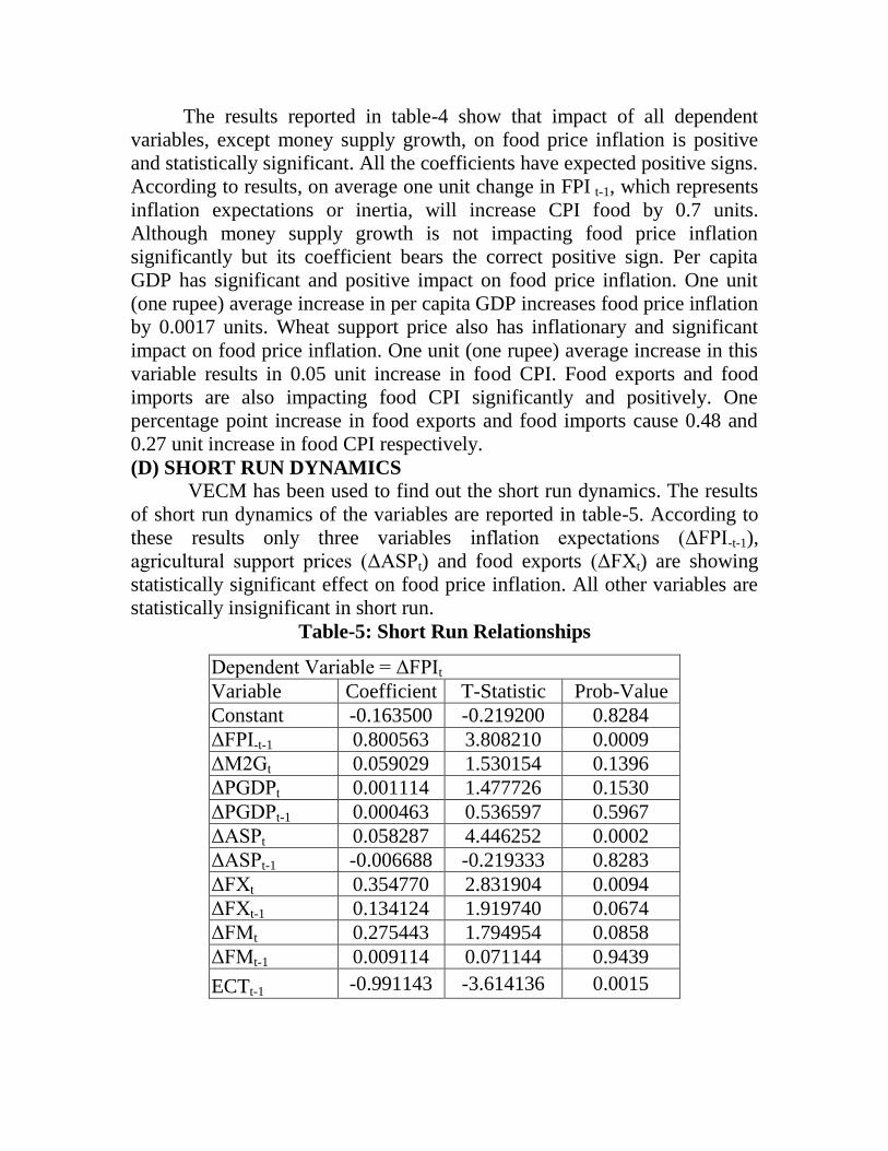
(D) SHORT RUN DYNAMICS

VECM has been used to find out the short run dynamics. The results

of short run dynamics of the variables are reported in table-5. According to

these results only three variables inflation expectations (ΔFPI-t-1),

agricultural support prices (ΔASPt) and food exports (ΔFXt) are showing

statistically significant effect on food price inflation. All other variables are

statistically insignificant in short run.

Table-5: Short Run Relationships

Dependent Variable = ΔFPIt

Variable Coefficient T-Statistic Prob-Value

Constant -0.163500 -0.219200 0.8284

ΔFPI-t-1 0.800563 3.808210 0.0009

ΔM2Gt 0.059029 1.530154 0.1396

ΔPGDPt 0.001114 1.477726 0.1530

ΔPGDPt-1 0.000463 0.536597 0.5967

ΔASPt 0.058287 4.446252 0.0002

ΔASPt-1 -0.006688 -0.219333 0.8283

ΔFXt 0.354770 2.831904 0.0094

ΔFXt-1 0.134124 1.919740 0.0674

ΔFMt 0.275443 1.794954 0.0858

ΔFMt-1 0.009114 0.071144 0.9439

ECTt-1 -0.991143 -3.614136 0.0015

R2= 0.915113

Adj-R2 = 0.874

F-Statistic= 22.54085

Prob(F-statistic)= 0.000

Durbin-Watson = 2.092

The error correction term of our short run model is also statistically

significant with a negative sign. It is another proof that long run relationship

exists among the variables we used in this study. The negative value of

coefficient of ECTt-1, which is (-0.9), indicates the very high speed of

convergence towards equilibrium. It may be justified because food price

inflation, even more than general inflation, is very sensitive to policy shocks

like administered prices (support prices), trade policy (export of food) and

inertia (inflation expectations). Empirical results of this study reveal that all

explanatory variables have positive relation with food price inflation. The

entire variables showed correct sign and are statistically significant except

money supply. Money supply affects food price inflation positively but its

impact is not significant. It shows food price inflation in Pakistan is not a

‘monetary phenomenon’. A number of empirical studies for Pakistan as well

as for other countries support the results about money supply (Tweeten,

1980; Bhattacharia and Lodh, 1990; Balkrishnan 1992, 1994; Hasan et al.

2005; Loaning et al. 2008). One year lag of food CPI is used to check the

impact of expectations about food price inflation. It is highly significant with

positive sign both in long run and short run. As food is the basic need of

human beings, people are very conscious about its future prices. They

develop their expectations on basis of current food prices and the past

experiences. Inflationary expectations are basic reasons of price-wage spiral

which creates inflationary effects for the economy. These findings are in line

with the studies of Hasan et al. 2005, Bernanke 2007, Loaning et al. 2008

and Ueda, 2009. Agriculture support prices are also affecting food price

inflation positively and significantly both in long run and short run. It is

generally considered that increase in support prices of wheat is responsible

for food price inflation in Pakistan. The results are in conformity with some

earlier studies (Balkrishnan, 1992; Khan and Qasim, 1996; Lorie and Khan

2006; Khan and Schimimelpfenning, 2006). Increase in per capita GDP as

proxy of growth has positive and significant impact on food price inflation.

In Pakistan services and manufacturing sectors are growing more rapidly as

compared to agriculture sector. Percentage share of these sectors in GDP is

increasing with the passage of time. Share of services sector in GDP was

41.9% in 1972 which increased to 53% in 2008. Percentage share of

manufacturing sector in GDP also improved from 15.8% to 19.1% during

1972 to 2008. The percentage share of agriculture in GDP is decreasing

gradually. It was 35.5% in 1972 which has decreased to 20.4% in 2008

(WDI, 2008). In this situation, per capita GDP has fairly positive relation

with food price inflation. Food imports and food exports also exert positive

and significant impact on food price inflation because prices and demand for

food items have been increasing at global level. Exchange rate depreciation

is also increasing the prices of food imports. Results of our study show that

food imports are inflationary in the long run only. In the short run food

imports do not affect food price inflation significantly. Khan and Qasim

(1996) also found the similar impact of import prices on inflation. Food

exports disturb supply situation in national markets resulting in inflation.

Food exports also increase food price inflation through inflation expectation

and hoarding channel.

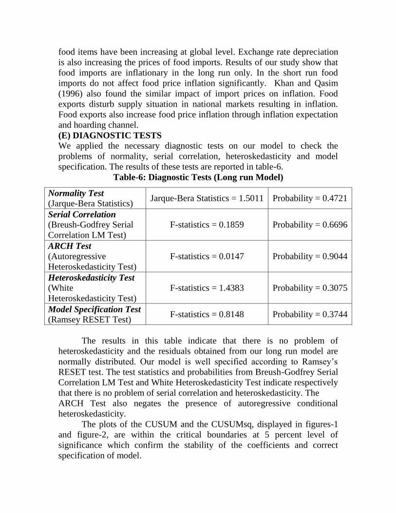
(E) DIAGNOSTIC TESTS We applied the necessary diagnostic tests on our model to check the

problems of normality, serial correlation, heteroskedasticity and model

specification. The results of these tests are reported in table-6.

Table-6: Diagnostic Tests (Long run Model)

Normality Test

(Jarque-Bera Statistics) Jarque-Bera Statistics = 1.5011 Probability = 0.4721

Serial Correlation

(Breush-Godfrey Serial

Correlation LM Test)

F-statistics = 0.1859 Probability = 0.6696

ARCH Test

(Autoregressive

Heteroskedasticity Test)

F-statistics = 0.0147 Probability = 0.9044

Heteroskedasticity Test

(White

Heteroskedasticity Test)

F-statistics = 1.4383 Probability = 0.3075

Model Specification Test

(Ramsey RESET Test) F-statistics = 0.8148 Probability = 0.3744

The results in this table indicate that there is no problem of

heteroskedasticity and the residuals obtained from our long run model are

normally distributed. Our model is well specified according to Ramsey’s

RESET test. The test statistics and probabilities from Breush-Godfrey Serial

Correlation LM Test and White Heteroskedasticity Test indicate respectively

that there is no problem of serial correlation and heteroskedasticity. The

ARCH Test also negates the presence of autoregressive conditional

heteroskedasticity.

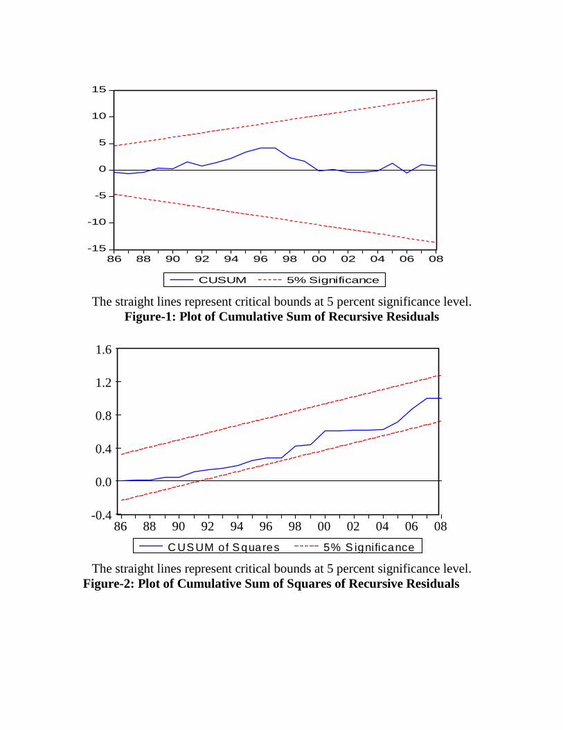
The plots of the CUSUM and the CUSUMsq, displayed in figures-1

and figure-2, are within the critical boundaries at 5 percent level of

significance which confirm the stability of the coefficients and correct

specification of model.

-15

-10

-5

0

5

10

15

86 88 90 92 94 96 98 00 02 04 06 08

CUSUM 5% Significance

The straight lines represent critical bounds at 5 percent significance level.

Figure-1: Plot of Cumulative Sum of Recursive Residuals

The straight lines represent critical bounds at 5 percent significance level.

Figure-2: Plot of Cumulative Sum of Squares of Recursive Residuals

-0.4

0.0

0.4

0.8

1.2

1.6

86 88 90 92 94 96 98 00 02 04 06 08

C U S U M o f S q u a r e s 5 % S i g n i f i c a n c e

5. CONCLUSION AND POLICY IMPLICATIONS

In the recent years, food price inflation has risen very sharply at

global level. It has increased the living cost of households especially in

developing countries like Pakistan which results in malnutrition and,

therefore, productivity losses. It hurts the poor more because they spend

more than half of their budget on food. In Pakistan, food inflation remained

9.9 % on average during the study period (1972-2008), some time as high as

34.7 % in 1974 and 26.6 % in 2008-09.

Time series data from 1972 to 2008 of relevant variables was used for

empirical analysis. First of all, stationarity of time series was checked by

using Augmented Dickey-Fuller (ADF) unit root test. All variables were

integrated of order one I(1) as they became stationary at their first

differences at 5% level of significance. As the variables had same order of

integration, therefore Johansen co-integration was applied to find the long-

run relationships. Maximum Eigen Statistics max and Trace Statistics trace

were used. Both statistics confirmed the existence of co-integration and

same number (two) of co-integrating vectors.

The impact of all dependent variables on food price inflation was positive

and statistically significant except money supply growth. All the coefficients

had expected positive signs.

The results revealed that both demand and supply side factors

determined food price inflation in Pakistan. However, on the basis of

empirical results we may conclude that food price inflation is not a monetary

phenomenon in Pakistan (money supply growth is statistically insignificant).

While the supply side factor or structural factors have dominant role in

determining the food prices.

Vector Error Correction Model (VECM) had been used for the

analysis of short run dynamics. In the short run, only inflation expectations,

support prices and food exports affected the food price inflation. The

negative value of coefficient of ECTt-1, which is (-0.9), indicated the very

high speed of convergence towards equilibrium.

Findings of the study show that ‘inflation inertia’ has dominant role in

determining food price inflation both in long run and short run in Pakistan.

There are various factors behind the inertia. These are: inflation

expectations, administered prices of energy (petroleum products, gas and

electricity) and agricultural products, government’s monetary policy and

fiscal policy. Therefore, there should be continuity and consistency in

government’s economic policies.

Support prices are the second major source of food price inflation in

Pakistan. Government should pursue a moderate policy in raising support

prices. Alternative to support price policy, government may provide

subsidies on inputs as on fertilizers, pesticides, diesel and electricity.

Government should also encourage and support farmers to adopt modern

technology for higher production with lower production cost.

Economic growth (increase in per capita GDP) is also contributing

towards food price inflation according to this study. It is because the

percentage share of services and manufacturing sectors to GDP is growing

rapidly as compared to agricultural sector in Pakistan. Government should

formulate proper policy for agriculture sector to fill the output gap.

Sufficient credit facilities should be provided through formal and informal

channel. Government should take measures to improve infrastructure,

agriculture markets and land ownership system. Modern technology should

be introduced to improve the production of food grains, meat, poultry and

dairy products.

According to our analysis, imports of food items are also inflationary

because of higher prices of food item at global level and exchange rate

depreciation. As a policy measure, we need to exploit our unrealized yield

potential in production of food items as God has gifted us with all necessary

resources.

This study reveals that food exports affect food price inflation

positively not only in the long run but also in the short run. Government

should ban the exports of food items until they are over and above the

domestic needs. For price stability in the country, buffer stocks of essential

food items like wheat, sugar and pulses should be maintained. There should

be maximum control on smuggling of wheat, rice and live stock to

neighboring countries.

Empirical results of this study prove that growth in money supply or

expansionary monetary policy does not affect food price inflation

significantly in Pakistan. In this situation it is suggested that government

should encourage the expansion in private sector credit, especially towards

the agricultural and its related sectors. There should be the availability and

easy access of loans for all farmers for all types of their needs such as

expenditure on the use of modern technology, inputs, marketing and storage

facilities. Increase in public expenditures on the provision of infrastructure

for rural areas will also be helpful for optimal utilization of the potential of

agriculture sector.

REFERENCES 1. Abhayartne, A. and Kasturi, K. M. (2008). Rising Food Prices: Are there

Solutions? Ground View, November 20, 2008.

2. Alderman, H. (2005). Linkages between Poverty Reduction Strategies and Child

Nutrition: An Asian Perspective. Economic and Political Weekly, 40(46), 4837-

4842.

3. Asian Development Bank (2008). Food Prices and Inflation in Developing

Asia: Is Poverty Reduction Coming to an End. Manila, Philippines: Asian

Development Bank.

4. Balkrishnan, P. (1992). Industrial Price Behavior in India: An Error-Correction

Model. Journal of Development Economics, 37(2), 309-326.

5. Balkrishnan, P. (1994). How Best to Model Inflation in India. Journal of Policy

Modeling, 16(6), 677-683.

6. Banerjee, A., Dolado, J. and Mestre, R. (1998). Error-correction Mechanism Test

for Co-integration in Single Equation Framework. Journal of Time Series

Analysis, 19(3), 267-283.

7. Baumol, W. (1967). Macroeconomics of Unbalanced Growth: The Anatomy of

Urban Crisis. American Economic Review, 57(3), 415-426.

8. Bernanke, B.S. (2007). Inflation Expectations and Inflation Forecasting. Remarks

at the NBER Monetary Economics Workshop.

9. Bhattacharya, B.B. and Lodh, M. (1990). Inflation in India: An Analytical Survey.

Artha Vijnana, 32(1), 25-68.

10. Bruno,G. S. and Babula (2005). Evolving Dynamic Relationships between the

Money Supply and Food-Based Prices in Canada and the United States. Canadian

Journal of Agricultural Economic, 42(2), 159-176.

11. Callen, T. and Chang, D. (1999). Modeling and Forecasting Inflation in India.

IMF Working Paper No. 99/119. Washington, D.C., USA: International Monetary

Fund.

12. Commodity Research Bureau (2009). Commodity Index Report. Volume 30, No.

27, Chicago, USA: Commodity Research Bureau.

13. Devadoss, S. and Meyers, W. H. (1987). Relative Prices and Money: Further

Results for United States. American Journal of Agricultural Economics, 69(4),

838-842.

14. Dickey, D.A. and Fuller, W.A. (1979). Distribution of the Estimation for

Autoregressive Time Series with Unit Root. Journal of the American Statistical

Association, 74(366), 427-431.

15. Dickey, D.A. and Fuller, W.A. (1981). Likelihood Ratio Statistics for

Autoregressive Time Series with a Unit Root. Econometrica, 49(4), 1057-1072..

16. Easterly, W. and Fischer, S.(2001). Inflation and Poor. Journal of Money, Credit

and Banking 33(2), 160-78.

17. Engle, R., and Granger, C. (1987). Co-integration and Error Correction:

Representation, Estimation, and Testing. Econometrica, 55(2), 251-276..

18. Friedman, M. (1968). The Role of Monetary Policy. American Economic Review,

58(1), 1-17.

19. Friedman, M. (1970). A Theoretical Framework of Monetary Analysis. Journal of

Political Economy, 78(2), 193-238.

20. Friedman, M. (1971). A Monetary Theory of Nominal Income. Journal of

Political Economy, 79(2), 323-337.

21. Government of Pakistan (2007). Pakistan Economic Survey 2006-07. Islamabad,

Pakistan: Finance Division, Government of Pakistan.

22. Government of Pakistan (2009). Pakistan Economic Survey 2008-09. Islamabad,

Pakistan: Finance Division, Government of Pakistan.

23. Granger, C. and Newbold, P. (1974). Spurious Regressions in Econometrics.

Journal of Econometrics, 2(2), 111-120.

24. Hasan, M. A., Khan, A. H., Pasha, H.A. and Rasheed, M.A. (1995). What

Explains the Current High Rate of Inflation in Pakistan. The Pakistan

Development Review, 34(4), 927 – 943.

25. International Food Policy Research Institute (2008). High Food Prices: The What,

Who and How of Proposed Policy Actions. (Annual Report) Washington, DC,

United States: International Food Policy Research Institute (IFPRI).

26. Johansen, S. (1988). Statistical Analysis of Co-integrating Vectors. Journal of

Economic Dynamics and Control, 12(3), 231-254.

27. Johansen, S. and Juselius, K. (1990). Maximum Likelihood Estimation and

Inference on Co-integration - with Applications to the Demand for Money.

Oxford Bulletin of Economics and Statistics, 52(2), 169-210.

28. Johson, H. K. (2008). Food Price Inflation Explanation and Policy Implications.

(Report for Bernard and Irene Foundation).

29. Khan, A. A., Bukhari, S. K. and Ahmad, Q. M. (2007). Determinants of Recent

Inflation in Pakistan. (Research Report No. 66). Karachi, Pakistan: Social Policy

and Development Center.

30. Khan, A. H. and Qasim, M.A. (1996). Inflation in Pakistan Revisited. The

Pakistan Development Review, 35(4), 747–59.

31. Khan, M. S. and Schimimelpfenning, A. (2006). Inflation in Pakistan. The

Pakistan Development Review, 45, 185–202.

32. Kremers, J.J.M., Ericson, N.R. and Dolado, J.J. (1992). The Power of

Cointegration Tests. Oxford Bulletin of Economics and Statistics, 54(3), 325-348.

33. Loening, L.J., Durevall, D., Birru, Y.A. (2009). Inflation Dynamics and Food

Prices in an Agricultural Economy: The Case of Ethiopia. University of

Gothenburg Working Paper No.347. Gothenburg, Sweden: University of

Gothenburg.

34. Lorie, H. and Khan, K.Y. (2006). What Determines the Domestic Prices of

Agricultural Commodities in Pakistan? The Pakistan Development Review, 45(4),

667–687.

35. Maynard, G. and Willy R. (1976). A World of Inflation. New York, USA:

Batsford.

36. Olivera, J. (1964). On Structural Inflation and Latin-American Structuralism.

Oxford Economic Papers, 16(3), 321-332.

37. Xuehua, P. Merchant, M. A., and Reed, M. R. (2004). Identifying Monetary

Impacts on Food Prices in China: AVEC Model Approach. Available at

http://ageconoresearch.umn.edu/bitstream/20315/1/sp04pe06.pdf.

38. Philips, P.C.B. (1986). Understanding Spurious Regressions in Econometrics.

Journal of Econometrics, 33(3), 311-340.

39. Saghaian, S. H., Reed, M.R. and Merchant, M.A. (2002). Monetary Impacts and

Over Shooting of Agricultural Prices in an Open Economy. American Journal of

Agricultural Economics, 84(1), 90-103

40. Schwartz, A. (1973). Secular Price Change in Historical Perspective. Journal of

Money, Credit and Banking, 5(1), 243-269.

41. Sharif, M., Farooq, U. and Bashir, A. (2000). Illegal Trade of Pakistan with

Afghanistan and Iran through Balochistan: Size, Balance and Loss to the Public

Exchequer. International Journal of Agriculture and Biology, 2(3), 199-203.

42. Streeten, P. (1962). Wages, Prices and Productivity. Kyklos, 15(4), 723-333.

43. Tweeten, L. G. (1980). Macroeconomics in Crises: Agriculture in an

Underachieving Economy. American Journal of Agricultural Economics, 62(5),

853-865.

44. Ueda, K. (2009). Determinants of Households’ Inflation Expectations. Discussion

Paper No. 2009-E-8. Tokyo,Japan: Institute for Monetary and Economic Studies

(IMES).

45. World Bank (2007). Quarterly Update. Beijing, China: Word Bank Office.