determinants of inflation in bangladesh: an econometric...
TRANSCRIPT
Journal of World Economic Research 2014; 3(6): 83-94
Published online November 20, 2014 (http://www.sciencepublishinggroup.com/j/jwer)
doi: 10.11648/j.jwer.20140306.13
ISSN: 2328-773X (Print); ISSN: 2328-7748 (Online)
Determinants of inflation in Bangladesh: An econometric investigation
Samim Uddin2, Md. Niaz Murshed Chowdhury
1, Dr. Mohammad Abul Hossain
3
1Department of Economics, University of Chittagong, Chittagong, Bangladesh 2Research Assistant, Department of Economics, South Dakota State University, Brookings, USA 3Professor, Department of Economics, University of Chittagong, Chittagong, Bangladesh
Email address: [email protected] (S. Uddin), [email protected] (Md. N. M. Chowdhury), [email protected] (Md. M. Uddin)
To cite this article: Samim Uddin, Md. Niaz Murshed Chowdhury, Dr. Mohammad Abul Hossain. Determinants of Inflation in Bangladesh: An Econometric
Investigation. Journal of World Economic Research. Vol. 3, No. 6, 2014, pp. 83-94. doi: 10.11648/j.jwer.20140306.13
Abstract: Both the increase and the decrease of inflation rate (General Price level) are like a two side sharpened razor in an
economy like Bangladesh. They both are harmful for an economy. Therefore, it has been attempted here to know about some
experimented determinants of inflation. Moreover, in this respect a well-known econometric technique, namely, Autoregressive
Distributed Lagged (ARDL) Model has been applied. By employing data series for 1972 to 2012, it has been indicated that the
gross domestic product (GDPt), money supply (M2t), and interest rate (IRt) of current year of Bangladesh as well as previous
year’s real exchange rate (RERt-1) and interest rate (IRt-1) have contributed to increase inflation in Bangladesh. It has also been
noticed that current year’s real exchange rate (RERt) in Dollar and previous year’s money supply (M2t) have contributed to
decrease the inflation rate. In our study, we emphasized on the significance of variables and availability of data because of
which some important determinants like unemployment rate (Ut), remittance (REMt) and oil price (PPt) have been ignored in
main model.
Keywords: ARDL Model, Diagnostic Test, Inflation Rate, Money Supply, Interest Rate, Real Exchange Rate
1. Introduction
Bangladesh, officially The People’s Republic of
Bangladesh, is a country in South Asia. It is bordered by
India on all sides except for a small border with Myanmar to
the far southeast and by the Bay of Bengal to the south.
Different types of natural disasters have visited Bangladesh
fluently. By some man created disasters like environment
pollution, unemployment, lack of effective investment,
inauspicious position of foreign trade and gradual increase of
food and non-food goods and service prices people are
awkward with their life. Inflation has materialized as a global
phenomenon in recent months largely reflecting the impact
of higher food and fuel prices and strapping demand
conditions especially in the emerging economies. In line with
global trends, Bangladesh also experienced rising inflation
with the 12-month average CPI inflation touching 10.96
percent in February 2012 (Bangladesh bank, 2012). The
present cycle of rising inflation is the longest in the history of
Bangladesh persisting for seven consecutive years, which in
earlier episodes, usually showed fluctuating movements with
the rising trend continuing for 2/3 years.
The economy of Bangladesh has been suffering from a
double-digit inflation. A shortage of oil production or energy
crisis world-wide, increase in energy prices and cost-of
production in combination with a demand-pull inflation from
expansionary economic policies have caused persistent
inflation. Altogether, these have created a supply-side
problem by decreasing the productivity. The situation of
Bangladesh has been aggravated due to political problems
and efforts for minimizing corruption and a lack of
confidence in business and manufacturing. It is hard to
assume that we can ever get back to the single digit inflation.
It is almost clear that we have to live with this double-digit
inflation. We must find out the avenue how to increase output
and income, aggregate production and supply of goods and
services in an effort to fight the inflation. The natural rate of
inflation from four to five per cent is accepted in almost any
developing country. Nevertheless, a double-digit inflation of
more than ten percent must have some reasons. Consumers
are worried about higher or increasing prices of their
consumer goods as their real income, purchasing power and

84 Samim Uddin et al.: Determinants of Inflation in Bangladesh: An Econometric Investigation
their standard of living is going down. Producers,
manufactures, businessmen and traders are overly concerned
about increasing prices of raw materials, energies including
electricity, gas and oil and the higher cost of production.
High rates of inflation distort economic performance,
making it mandatory to identify the causing factors. Several
internal and external factors, such as the printing of money
by the government, a rise in production and labor costs, high
lending rates, a drop in the exchange rate, increased taxes or
wars, can cause inflation. This study aims at ascertaining the
determinants of inflation of Bangladesh by applying the
Autoregressive Distributive Lagged Model (ARDL).
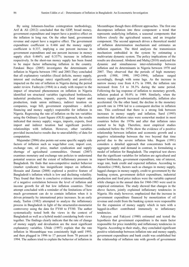
Figure 1.1. Fluctuation of Inflation Rate of Bangladesh (Jan’95-Jan’13)
Data Source: Bangladesh Bureau of Statistics.
The inflation rate in Bangladesh was recorded at 7.86
percent in May of 2013. The Bangladesh Bureau of Statistics
reports the inflation rates in Bangladesh. Historically, from
1994 till 2013, Bangladesh’s inflation rate averaged 6.60
Percent reaching an all time high of 12.71 Percent in
December of 1998 and a record low of -0.02 Percent in
December of 1996. In Bangladesh, the inflation rate
measures a broad rise or fall in prices that consumers pay for
a standard basket of goods.
The market intermediaries are the last agents to charge
higher prices. Recently most of our economists think that
devaluation or depreciation of the exchange rate of Taka is
another cause of inflation, with whom the Governor of
Bangladesh Bank (BB) disagreed. It matters little how the
devaluation is related to inflation rate. We are in an economic
stage of recession with lower output and income, higher
unemployment and an unacceptably high instability in prices
and inflation. We simply cannot afford to have a
contractionary monetary policy to increase the exchange rate
or value of Taka. On the other hand, contractionary monetary
policy will further lower the output and income, increase
unemployment and lower purchasing power and further
aggravate the situation, and may not be able to decrease the
cost-push inflation. Since independence, Bangladesh has
been under a persistent inflationary pressure caused mainly
by excess money supply as (Hossain, 2002). The popular
judgment about the costs of inflation is that inflation makes
everyone worse off by trading off the purchasing power of
incomes, eroding living standards and adding, in many ways,
to life’s uncertainties (Lipsey et al. 1982). Broadly speaking,
the primary effects of inflation are the redistribution of
income and wealth associated with unanticipated inflation,
which is likely to affect economic activities and resource
allocation of the country (Taslim, 1980).
Different schools of thought provide different views on
what actually causes inflation. However, there is a general
agreement amongst economists that economic inflation may
be caused by either an increase in the money supply or a
decrease in the quantity of goods being supplied. The
proponents of the Demand Pull theory attribute a rise in
prices to an increase in demand in excess of the supplies
available. An increase in the quantity of money in circulation
relative to the ability of the economy to supply leads to
increased demand-fuelling prices. The case is of too much
money chasing too few goods. An increase in demand could
also be a result of declining l interest rates, a cut in tax rates
or increased consumer confidence. The Cost Push theory, on
the other hand, states that inflation occurs when the cost of
producing rises and the increase is passed on to the
consumers. The cost of production can rise because of rising
labor costs or when the producing firm is a monopoly or
oligopoly and raises prices; cost of imported raw material
rises due to exchange rate changes, and external factors, such
as natural calamities or an increase in the economic power of
a certain country. An increase in indirect taxes can also lead
to increased production costs. A classic example of cost-push
or supply-shock inflation is the oil crisis that occurred in the
1970s, after the OPEC raised oil prices. Now a days due to
oil price being increased by importers of petroleum and
reducing subsidy on imported oil Bangladesh economy
experienced double-digit inflation in previous few years.
Since oil is used in every industry and increasing demand of
oil in Quick Rental Power plant of Bangladesh accelerate the
oil price in domestic market, a sharp rise in the price of oil
leads to an increase in the prices of all commodities.
The main purpose of the study is to identify the causes of
inflation of developing countries like Bangladesh. Like other
monetary authorities of developing countries, the central
bank of Bangladesh and Bangladesh govt. are anxious with
the policy types that may control the hyperinflation1. As a
result, the determinants of inflation play a vital rule to policy
makers. A list of examined determinants may make easy to
control inflation.
More specifically, the study hubs of the following
objective
� To have more clear knowledge about the techniques,
rules and standards of measurement of inflation;
� To assess out the current situation of Inflation in
Bangladesh;
� To compare the inflation fluctuation and its impact on
economy periodically;
� To compare the inflation fluctuation among neighbor
countries;
1 A very rapidly accelerating inflation is also known as runaway inflation or
galloping inflation. This usually leads to the breakdown of the country's monetary
system as the existing currency may have to be withdrawn and a new one
introduced.
Journal of World Economic Research 2014; 3(6): 83-94 85
� To explore the implication of forecasting techniques in
inflation of Bangladesh;
� To detect the causes relevant to inflation and fluctuation;
2. Literature Review
Numerous studies attempted to estimate short run and long
run relationships between inflation rate and its determinants
in different countries applying different theoretical and
methodological constructs. In this section, some of these
studies are summarized in terms of their methodologies and
findings in the basis of publishing year. There have been very
few studies on forecasting inflation in Bangladesh and other
developing countries using time series techniques. A review
of the selected empirical studies on the determinants of
inflation in Bangladesh reveals varied results. Most studies
are based on qualitative analysis of the inflationary trends in
Bangladesh. Thus, factors related to short-run and long-run
inflation elasticities have not been adequately explored.
Mortaza and Rahman (2008) dissected the relationship
between import and domestic prices in Bangladesh during
2000-2008. Using monthly data, they investigated the
relationship between domestic supplies, pass through
elasticity, and alleged that commodities with higher share of
domestic supply face a lower pass-through elasticity of
import prices on domestic prices. The results suggest that it is
important for policies in Bangladesh to correctly align the
exchange rate and trade related policies in the short run to
domestic realities coupled with the long run policy of
increasing domestic production as the most effective strategy
to ensure domestic price stability. Ahmed and Mortaza (2005)
attempt an assessment of empirical evidence through the co-
integration and error correction models using annual data set
of Bangladesh on real GDP and CPI for the period of 1980 to
2005. The empirical evidence demonstrated that there existed
a statistically significant long-run negative relationship
between inflation and economic growth for the country as
indicated by a statistically significant long-run negative
relationship between CPI and real GDP. In Thailand Tao Sun
(2004) developed an approach for forecasting core inflation
using monthly data from May 1995 to October 2003. The
seasonally adjusted, monthly percent changes in Thailand’s
consumer price index after removing its raw food and energy
components is used as the dependent variable. Hafer and
Hein (2005) compared the relative efficiency of the widely
used interest rate based forecasting model and univariate
time series model based on monthly data from the United
States, Belgium, Canada, England, France and Germany for
the sample period from 1978 to 1986. Using monthly data on
the Euro rates and the consumer price index (CPI) their
results indicate that time series forecast of inflation model
produces equal or lower forecast errors and has unbiased
predictions than the interest rate based forecasts. Gavin and
Kevin (2006) using Stock Dynamic Factor Models (DFM)
forecast inflation and output with three alternative processes:
a benchmark autoregressive model; a random walk; and a
constant that presumes a fixed rate of growth of prices and
output over the forecast horizon 3, 12 and 24 months with the
monthly data from January 1978 to December 1996.
Faisal (2012) suggests that the long-time lag between
monetary policy announcement and policy action, it is
difficult for policymakers to coordinate properly their
strategies. Under such situation, forecasting future inflation
can assist policymakers in formulating their strategies. Along
with the time lag, in reality inflation is often multi causal and
prime cause of inflation can vary from year to year. Raihan
and Fatema (2007) reviewed a number of hypotheses put
forward by the economists, policy makers and donor
agencies, like IMF, World Bank and ADB, with regard to the
causes of inflation in Bangladesh. They found that both
demand-side and supply-side factors such as price hike of
food and non-food items have significant influence on the
rising trend of inflation in Bangladesh. Kabundi (2011) tried
to identify the main features underlying inflation in Uganda,
both in the long -run and short-run, using monthly data from
January 1999 to October 2010. The author ran a single-
equation Error Correction Model (ECM) based on the
quantity theory of money including both external and
domestic variables. Finally, they concluded that evidence of
inflation inertia which can be attributed to expectations of
agents and/or inflation persistence. Totonchi (2011)
attempted to review and analyze the competing theories of
inflation. The theoretical survey in this research work yielded
a six-blocked schematization of origins of inflation;
monetary shocks, Demand side, supply-side (or real) shocks,
structural and political factors (or the role of institutions). It
appeared that inflation is the net result of sophisticated
dynamic interactions of these six groups of explanatory
factors. That is to say, inflation is always and everywhere a
macroeconomic and institutional phenomenon.
Kozo & Ueda (2009) tried to investigate the determinants
of households’ inflation expectations in Japan and the United
States. They estimated a vector auto-regression model in
which the four endogenous variables are inflation
expectations, inflation, the short-term nominal interest rate
and the output gap, with energy prices and (fresh) food prices
being exogenous. Short-term nonrecursive restrictions are
imposed taking account of simultaneous codependence
between realized inflation and expected inflation. They find,
first, that responding not only to changes in energy prices and
food prices but also to monetary policy shocks, inflation
expectations adjust more quickly than does realized inflation.
Ratnasiri (2006) attempted to examine the determinants of
inflation for Sri Lanka over the period 1980 – 2005 using VAR
based co-integration approach. The findings indicate money
supply growth and the increases in rice price are the most
important determinants of inflation in Sri Lanka in the short
run and long run. The effect of GDP growth and exchange rate
depreciation on inflation has been found to be negligible and
statistically not significant. The short-run effect of money
growth, rice price and exchange rate effect on inflation is
statistically significant. However GDP growth is not
significant in short run too. It is obvious that the supply side
effect on inflation in Sri Lanka is reflected through rice prices.
86 Samim Uddin et al.: Determinants of Inflation in Bangladesh: An Econometric Investigation
By using Johansen-Juselius cointegration methodology,
Arif & Ali (2012) concluded that the GDP, broad money,
government expenditure and import have a positive effect on
the inflation in long run. On the other hand, government
revenue and export have a negative effect. The government
expenditure coefficient is 0.466 and the money supply
coefficient is 0.337, implying a one percent increase in
government expenditure and one percent increase in money
supply elicit 0.466% and 0.337% increase in inflation
respectively. In the short-run money supply has been found
to be major factor influencing inflation in the country.
Fatukasi Bayo (2005) investigates the determinants of
inflation in Nigeria between 1981 and 2003.They concluded
that all explanatory variables (fiscal deficits, money supply,
interest and exchange rates) significantly and positively
impacted on the rate of inflation in Nigeria during the period
under review. Fashoyin (1984) in a study with respect to the
impact of structural phenomenon on inflation in Nigeria
identified ten structural variables (agricultural bottlenecks,
industrial production, imports, exports, food import and
production, trade union militancy, indirect taxation on
companies, wage bill, government expenditure – deficit
financing and money supply) responsible for inflation in
Nigeria. Regressing the rate of inflation on the ten variables
using the Ordinary Least Square (OLS) approach, the results
indicated that money supply; wages, imports, exports, food
import and indirect taxation had significant positive
relationships with inflation. However, other variables
provided inconclusive results due to unavailability of data for
computation.
Majumdar (2006) also points out some specific supply side
factors of inflation such as wage/labor cost, import cost,
exchange rate, oil price, market syndication and supply
shortage of agricultural commodities. Osmani (2007)
examines monetary and exchange rate policies to understand
potential sources and the extent of inflationary pressure in
Bangladesh. He finds that non-competitive market behavior
(market syndicate) has insignificant impact on inflation.
Hossain and Zaman (2008) explored a positive feature of
Bangladesh‘s inflation which is low and declining volatility.
They found that there is conclusive evidence internationally
of a negative correlation between the level of inflation and
income growth for all but low inflation countries. Their
attempt concluded with a reminder of the limitations of how
much government can do to contain inflation when it is
driven primarily by international price increases. In an early
study, Taslim (1982) attempted to analyze the inflationary
process in Bangladesh in light of the structuralist-monetarist
controversy using the data for FY60 to FY80. The author
systematically tested both the views in the context of
Bangladesh as well as a hybrid model considering both views
together. The findings clearly indicate that the rate of change
of money supply and devaluation are the most significant
explanatory variables. Ubide (1997) explain that the rate
inflation in Mozambique was consistently high until 1995,
and then plugged in 1996 to 17 percent from 70 percent in
1994. The authors tried to explain the behavior of inflation in
Mozambique though there different approaches. The first one
decomposes inflation into three component: a trend that
represents underlying inflation, a seasonal components that
follows closely the agricultural season, and an irregular
component. The second approach drives a theoretical model
of inflation determination mechanism and estimates an
inflation equation. The third analyzes the transmission
mechanism embedded in the system by estimating a
multivariate dynamic system. The policy implications of the
results are discussed. Abidemi and Maliq (2010) analyzed the
dynamic and simultaneous inter-relationship between
inflation and its determinants in Nigeria between 1970 and
2007. They observed that the periods of high monetary
growth (1988, 1990, 1992-1994), inflation surged
accordingly, though with some lags. As the increase in
narrow money rose from 4.1% in 1988, the inflation rate
increased from 5.4 to 38.3% during the same period.
Following the lag response of inflation to monetary growth,
inflation peaked at 50.0% in 1989. Similarly, when the
money supply growth increased substantially, inflation also
accelerated. On the other hand, the decline in the monetary
growth rate in 1994 led to a consequent decline in inflation
rate. This confirmed that there is a strong link between
increases in money supply and inflation. Sarel (1995)
mentions that inflation rates were somewhat modest in most
countries before the 1970s and after that inflation rates
started to be high. Therefore, most empirical studies
conducted before the 1970s show the evidence of a positive
relationship between inflation and economic growth and a
negative relationship between the two beyond that time
period due to the severe inflation hike. Begum (1991)
considers a detailed approach that concentrates both on
aggregate supply and demand in contrast, in formulating a
model of inflation for Bangladesh. The empirical test shows
that the significant variables for inflation are agricultural and
import bottlenecks, government expenditure, rate of interest,
wage rate, bank credit and expected inflation. According to
Akinnifesi (1984), factors such as changes in money supply,
lagged changes in money supply, credit to government by the
banking system, government deficit expenditure, industrial
production and food price indices were the variable captured
while changes in the annual data for 1960-1983 were used in
empirical estimation. The study showed that changes in the
above factors, jointly explained inflationary tendencies in
Nigeria. His study however, emphasized that the increase in
government expenditure financed by monetization of oil
revenue and credit from the banking system were responsible
for the expansion of money supply which in turn with a
lagged-in-effect contributed immensely to inflationary
tendencies.
Adeyeye and Fakiyesi (1980) estimated and tested the
hypothesis that government expenditure is the main factor
responsible for price instability and inflationary tendencies in
Nigeria. According to their study,, they concluded significant
positive relationship between inflation rate and money supply,
government expenditure and bank credit was established but
the relationship of inflation rate with growth of government
Journal of World Economic Research 2014; 3(6): 83-94 87
revenue was unclear. Ahmed (2009) examines the sources of
inflation in Bangladesh taking into account both demand-side
and supply-side factors to explain the inflationary trend. He
finds that inward remittances, government debt, inflation
inertia, non-competitive market behavior, food and oil prices
affect inflation to a large extent. Mallik and Chowdhury
(2001) have examined the short-run and long-run dynamics
of the relationship between inflation and economic growth
for four South Asian economies: Bangladesh, India, Pakistan,
and Sri Lanka. Applying co-integration and error correction
models to the annual data retrieved from the International
Monetary Fund (IMF) and International Financial Statistics
(IFS). They found two motivating results. First, the
relationship between inflation and economic growth is
positive and statistically significant for all four countries.
Second, the sensitivity of growth to changes in inflation rates
is smaller than that of inflation to changes in growth rates.
Judson and Orphanides (1999) have estimated a non-linear
relationship and discovered structural breaks for many
developing countries including Bangladesh. These varied
findings, therefore, deserve further investigation for policy
implications. Besides, it is argued that an individual country
study should provide more reliable estimates than cross-
country studies as country-specific relevant variables can be
controlled properly and homogeneity can also be maintained.
Different demand and supply responses for policy changes in
different countries might result in different economic
outcomes and provide misleading results under cross-
sectional data. Temple (2000) pointed out that in cross-
country studies comprising relatively dissimilar developing
countries, inflationary impacts might differ and therefore,
extrapolation requires more caution. He further argued, citing
findings of several studies that the detection and significance
of some relationships change when cross-section instead of
annual panel data is used or if the time-horizon is altered.
Bangladesh is under pressure from the international lending
agencies (IMF, the World Bank and ADB) to reduce its
inflation rates in order to boost economic growth.
3. Data
This analysis is mainly based on secondary information. It
is suggested that combining secondary data from various
sources may increase the validity of the information.
Secondary data have been collected mainly from official
sources. Suitable data have been extracted, organized,
analyzed, illustrated and interpreted in the study with proper
reasoning, analytical judgment, clarification and explanation.
Research has been conducted on the basis of 1972-2012
inflation data frame in the context of Bangladesh. A time
series model is useful in examining the dynamic
determinants of economic series. The basic underlying
assumption in time series forecasting is that the set of casual
factors (Macroeconomic fundamentals) that operated on the
dependent variable in the past will exhibit similar influence
in some repetitive fashion in the future. In this research
historical yearly national consumer price indices (general)
data from (1972-2012) of Bangladesh will be analyzed. In
some previous studies of inflation forecasting of Bangladesh,
emphasis has been given on testing economic theory and on
empirical analysis. Even though some of these studies have
been used as an input into the forecasting process, they have
not been subject to rigorous forecast evaluation techniques.
This paper set out to redress this deficiency and explicitly use
time series techniques solely for forecasting purposes. All the
figures that were used in this study were collected from the
following publications. Bangladesh Bank Annual Report,
published by Bangladesh Bank. Bangladesh Economic
Survey, various issues, published by the Ministry of Finance.
Economic Trends (monthly), published by the Statistics
Department of the Central Bank of Bangladesh, official
website of the Central Bank, Ministry of Finance and Export
Promotion Bureau of Bangladesh. The World Economic
Outlook 2012, published by The International Monetary
Fund. Asian Development Bank (ADB) database. World
Bank databank (World Development Indicator, WDI).
Official website of World Bank. I have also checked
published books on economic issues, working papers, reports,
research monographs, journals and research works that are
relevant to the study.
The central objective of the ARDL approach to modeling
is to assess the inflationary potential of an economy through
evaluating the characteristics of its monetary conditions. The
ARDL type of models is based on the combination of long-
term determinants of the price level with short-term changes
in inflation in the economy.
In time series models, a substantial period of time may
pass between the economic decision-making period and the
final impact of a change in a policy variable. One can say
that it is the nature of economic relationships that the
adjustment of Y to changes in X is distributed widely through
time. If the appropriate decision and response period is
sufficiently long, lagged explanatory variables should be
included explicitly in the model.
One way to model the dynamic responses is to include
lagged values of X on the right hand side of the regression
equation; this is the basis of the distributed lag model, in
which a series of lagged explanatory variables account for
the time adjustment process. The (finite) distributed-lag
model takes the form:
�� = ���� + ����� + ��� +⋯+ ����� + ���� + �� Given the above model, if the explanatory (input) variable
x undergoes a one unit change (impulse) in some period t;
then the immediate impact on y is given by β0; β1 is the
impact on y after one period, β2 is the impact after two
periods, and so on. The final impact on y is βk and it occurs
after k periods. So speaking, it takes k periods for the full
effects of the impulse to be realized. The sequence of
coefficients {β0;β1; β2; …; βk} constitutes the impulse
response function of the mapping from Xt to Yt. Furthermore,
the dynamic behavior of an economy can reveal itself
through a dependence of the current value of an economic
variable on its own past values. Specifically, models of how
88 Samim Uddin et al.: Determinants of Inflation in Bangladesh: An Econometric Investigation
decision makers’ expectations are formed, and how they react
to changes in the economy, result in the value of yt depending
on lagged Y’s. Therefore, an alternative way to capture the
dynamic component of economic behavior is to include
lagged values of the dependent variable on the right-hand
side of the regression together with the exogenous variable.
In time-series econometric modeling, a dynamic
regression will usually include both lagged dependent and
independent variables as regressors:
�� = �� + ���� + ���� + ���� +⋯+ ����� + ���� + �� The above model is called the autoregressive distributed-
lag model, abbreviated as ARDL(p,k). ARDL of order 1 in
autoregression and order 1 in distributed lags:
ARDL(1,1) model is defined as M1. The values of p and k
(i.e how many lags of Y and X will be used) are chosen (i) on
the basis of the statistical significance of the lagged variables,
and (ii) that the resulting model is well specified (e.g. it does
not suffer from serial correlation).
As mentioned earlier, the motive is to find out the
determinants of inflation in Bangladesh. For this purpose,
several steps have been undertaken in the model specification.
We have completed the Stationary Test of all data series and
the results are presented below. However, many factors have
effect on inflation. Due to failure in stationary test and
insufficient data series, we have to ignore some important
factors like unemployment etc. In addition to this, we have
considered some proxy variables that are highly correlated
with considered variables. A brief is mentioned before those
are being considered as tested determinants of inflation.
4. Empirical Result
4.1. Testing for Stationarity in Data
A random time series is said to be stationary if its mean
and variance constant over time and the value of covariance
between two time periods depends only the distance between
the two time periods and not on the actual time at which the
variance is computed (Gujarti,1995). In order to check for
the time series properties stationary of the variables, the
widely applied unit root test such as Augmented Dccky –
Fuller (1981) and Philips-Perrron (1988) tests have been used.
One way of removing non-stationarity is through the method
of differencing. Unit Root test has been conducted to find out
the stationarity of the considered series like GDP, interest
rate, real exchange rate etc. The Augmented Dickey Fuller
Test (ADF) and Philips-Perron have been used to check the
existence of unit root of GDP series of Bangladesh the
method. The null and the alternatives are:
Ho: Consumer Price Index series have unit root;
Ha: Consumer Price index series do not follow unit root
Here, if and only if the P-value from ADF test is greater
than 0.05 or 5%, the null hypothesis (Ho) is accepted.
Otherwise, the null hypothesis will be rejected.
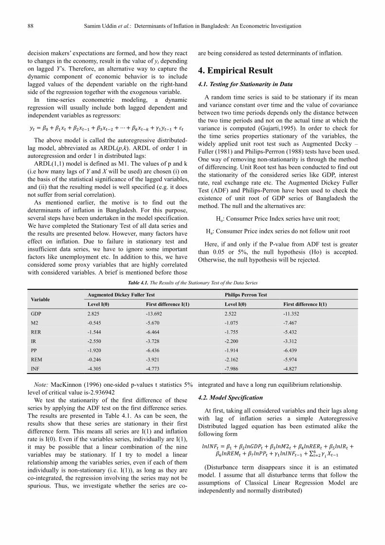
Table 4.1. The Results of the Stationary Test of the Data Series
Variable Augmented Dickey Fuller Test Philips Perron Test
Level I(0) First difference I(1) Level I(0) First difference I(1)
GDP 2.825 -13.692 2.522 -11.352
M2 -0.545 -5.670 -1.075 -7.467
RER -1.544 -6.464 -1.755 -5.432
IR -2.550 -3.728 -2.200 -3.312
PP -1.920 -6.436 -1.914 -6.439
REM -0.246 -3.921 -2.162 -5.974
INF -4.305 -4.773 -7.986 -4.827
Note: MacKinnon (1996) one-sided p-values t statistics 5%
level of critical value is-2.936942
We test the stationarity of the first difference of these
series by applying the ADF test on the first difference series.
The results are presented in Table 4.1. As can be seen, the
results show that these series are stationary in their first
difference form. This means all series are I(1) and inflation
rate is I(0). Even if the variables series, individually are I(1),
it may be possible that a linear combination of the nine
variables may be stationary. If I try to model a linear
relationship among the variables series, even if each of them
individually is non-stationary (i.e. I(1)), as long as they are
co-integrated, the regression involving the series may not be
spurious. Thus, we investigate whether the series are co-
integrated and have a long run equilibrium relationship.
4.2. Model Specification
At first, taking all considered variables and their lags along
with lag of inflation series a simple Autoregressive
Distributed lagged equation has been estimated alike the
following form
������ = �� + ������� + �����2� + �������� + ������� +�������� + ������� + �������� +∑ �!" ! #��
(Disturbance term disappears since it is an estimated
model. I assume that all disturbance terms that follow the
assumptions of Classical Linear Regression Model are
independently and normally distributed)
Journal of World Economic Research 2014; 3(6): 83-94 89
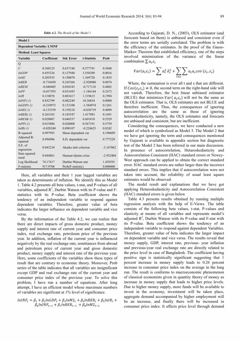
Table 4.2. The Result of the Model 1
Model 1
Dependent Variable: LNINF
Method: Least Squares
Variable Coefficient Std. Error t-Statistic Prob
Q
C 0.368125 0.637180 0.577741 0.5688
lnGDP 0.455236 0.127940 3.558209 0.0016
lnM2 0.205555 0.150070 1.369728 0.1835
lnRER -0.718450 0.245366 -2.928080 0.0074
lnREM -0.040405 0.056343 -0.717118 0.4802
lnPP -0.037593 0.031693 -1.186144 0.2472
lnIR 0.110078 0.083417 1.319615 0.1994
lnINF(-1) 0.852799 0.082249 10.36854 0.0000
lnGDP(-1) -0.210973 0.133108 -1.584974 0.1261
lnM2(-1) -0.133539 0.159218 -0.838719 0.4099
lnRER(-1) 0.263103 0.185547 1.417983 0.1691
lnREM(-1) 0.028007 0.046537 0.601818 0.5529
lnPP(-1) 0.015886 0.028008 0.567191 0.5759
lnIR(-1) -0.020240 0.090107 -0.224623 0.8242
R-squared 0.997993 Mean dependent var 4.190609
Adjusted R-
squared 0.996906 S.D. dependent var 0.777228
S.E. of
regression 0.043234 Akaike info criterion -3.167062
Sum squared
resid 0.044861 Hannan-Quinn criter. -2.952404
Log likelihood 74.17417 Durbin-Watson stat 1.429291
F-statistic 917.9708 Prob(F-statistic) 0.000000
Here, all variables and their 1 year lagged variables are
taken as determinants of inflation. We identify this as Model
1. Table 4.2 presents all beta values, t-stat, and P-values of all
variables, adjusted R2, Durbin Watson with its P-value and F-
statistics with its P-value. Beta coefficient shows the
tendency of an independent variable to respond against
dependent variables. Therefore, greater value of beta
indicates the larger influence on dependent variable and vice
versa.
By the information of the Table 4.2, we can realize that
there are direct impacts of gross domestic product, money
supply and interest rate of current year and consumer price
index, real exchange rate, petroleum price of the previous
year. In addition, inflation of the current year is influenced
negatively by the real exchange rate, remittances from abroad
and petroleum price of current year and gross domestic
product, money supply and interest rate of the previous year.
Here, some coefficients of the variables show these types of
result that are contrary to economic theory. Moreover, Prob
series of the table indicates that all variables are insignificant
except GDP and real exchange rate of the current year and
consumer price index of the previous year. To solve this
problem, I have run a number of equations. After long
attempt, I have an efficient model whose maximum numbers
of variables are significant at 1% level of significance.
������ = �� + ������� + �����2� + �������� + ������� +��������� + ��������� + �%���2��
According to Gujarati, D. N., (2003), OLS estimator (and
forecasts based on them) is unbiased and consistent even if
the error terms are serially correlated. The problem is with
the efficiency of the estimates. In the proof of the Gauss-
Markov Theorem that established efficiency, one of the steps
involved minimization of the variance of the linear
combination ∑&���
'&()&���* =+&� ,- +++&�&-./0�1-
)��, �-*
Where, the summation is over all t and s that are different.
If3/0)���-* ≠ 0, the second term on the right-hand side will
not vanish. Therefore, the best linear unbiased estimator
(BLUE) that minimizes '&()&���* will not be the same as
the OLS estimator. That is, OLS estimates are not BLUE and
therefore inefficient. Thus, the consequences of ignoring
autocorrelation are the same as those of ignoring
heteroskedasticity, namely, the OLS estimates and forecasts
are unbiased and consistent, but are inefficient.
Considering the consequences, we have conducted a new
model of which is symbolized as Model 3. The Model 2 that
we have got ignoring the term and consequences mentioned
by Gujarati is available in appendix section but diagnostic
test of the Model 2 has been referred in our main discussion.
In presence of autocorrelation, Hetaroskedasticity and
Autocorrelation Consistent (HAC) standard errors or Newey-
West approach can be applied to obtain the correct standard
error. HAC standard errors are rather larger than the incorrect
standard errors. This implies that if autocorrelation were not
taken into account, the reliability of usual least square
estimates would be observed.
The model result and explanations that we have got
applying Hetaroskedasticity and Autocorrelation Consistent
(HAC) standard errors is given below
Table 4.3 presents results obtained by running multiple
regression analysis with the help of E-Views. The table
consists of the following beta values, t-stat, P-values and
elasticity at means of all variables and represents model’s
adjusted R2, Durbin Watson with its P-value and F-stat with
its P-value. Beta coefficient shows the tendency of an
independent variable to respond against dependent Variables.
Therefore, greater value of beta indicates the larger impact
on dependent variable and vice versa. The results reveal that
money supply, GDP, interest rate, previous- year inflation
and previous-year real exchange rate are directly related to
the price level in case of Bangladesh. The coefficient having
positive sign is statistically significant suggesting that 1
percent increase in money supply leads to 0.26 percent
increase in consumer price index on the average in the long
run. The result is conforms to macroeconomic phenomenon
of classical economists given in quantity theory of money as
increase in money supply that leads to higher price levels.
Due to higher money supply, more funds will be available to
invest in the economy, investment will be taken place,
aggregate demand accompanied by higher employment will
be an increase, and finally there will be increased in
consumer price index. It affects price level through demand
90 Samim Uddin et al.: Determinants of Inflation in Bangladesh: An Econometric Investigation
side. GDP is inducing consumer price index at 1 percent
level of significance implying that consumer price index will
increase by 0.23 percent due to 1 percent increase in gross
domestic product on the average in the long run. In the same
manner, if interest rate rises by 1 percent, price level will
increase by 0.09 percent on the average in the long run. The
results show that real exchange rate and previous year’s
money supply is found to be inversely related to the price
level in case of Bangladesh. The coefficient having negative
sign is statistically significant suggesting that 1 percent
decrease in the previous-year money supply and real
exchange rate leads to 0.25 percent and 0.89 percent increase
respectively in consumer price index on the average in the
long run.
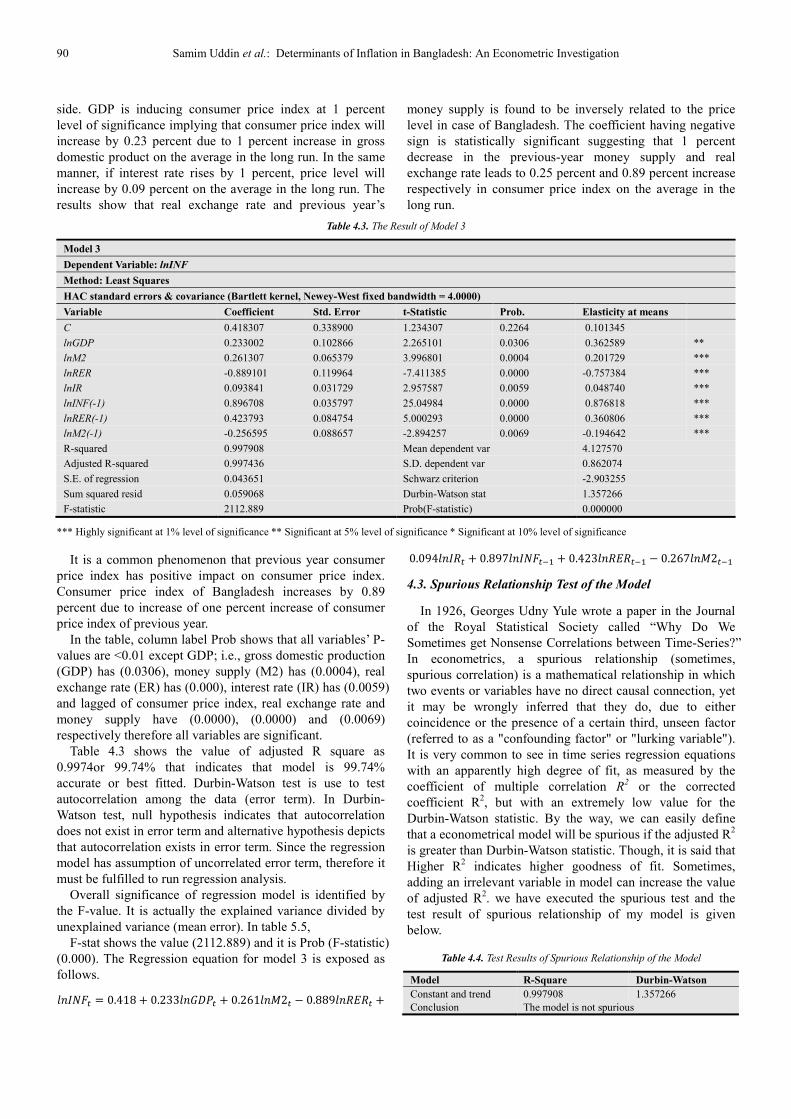
Table 4.3. The Result of Model 3
Model 3
Dependent Variable: lnINF
Method: Least Squares
HAC standard errors & covariance (Bartlett kernel, Newey-West fixed bandwidth = 4.0000)
Variable Coefficient Std. Error t-Statistic Prob. Elasticity at means
C 0.418307 0.338900 1.234307 0.2264 0.101345
lnGDP 0.233002 0.102866 2.265101 0.0306 0.362589 **
lnM2 0.261307 0.065379 3.996801 0.0004 0.201729 ***
lnRER -0.889101 0.119964 -7.411385 0.0000 -0.757384 ***
lnIR 0.093841 0.031729 2.957587 0.0059 0.048740 ***
lnINF(-1) 0.896708 0.035797 25.04984 0.0000 0.876818 ***
lnRER(-1) 0.423793 0.084754 5.000293 0.0000 0.360806 ***
lnM2(-1) -0.256595 0.088657 -2.894257 0.0069 -0.194642 ***
R-squared 0.997908 Mean dependent var 4.127570
Adjusted R-squared 0.997436 S.D. dependent var 0.862074
S.E. of regression 0.043651 Schwarz criterion -2.903255
Sum squared resid 0.059068 Durbin-Watson stat 1.357266
F-statistic 2112.889 Prob(F-statistic) 0.000000
*** Highly significant at 1% level of significance ** Significant at 5% level of significance * Significant at 10% level of significance
It is a common phenomenon that previous year consumer
price index has positive impact on consumer price index.
Consumer price index of Bangladesh increases by 0.89
percent due to increase of one percent increase of consumer
price index of previous year.
In the table, column label Prob shows that all variables’ P-
values are <0.01 except GDP; i.e., gross domestic production
(GDP) has (0.0306), money supply (M2) has (0.0004), real
exchange rate (ER) has (0.000), interest rate (IR) has (0.0059)
and lagged of consumer price index, real exchange rate and
money supply have (0.0000), (0.0000) and (0.0069)
respectively therefore all variables are significant.
Table 4.3 shows the value of adjusted R square as
0.9974or 99.74% that indicates that model is 99.74%
accurate or best fitted. Durbin-Watson test is use to test
autocorrelation among the data (error term). In Durbin-
Watson test, null hypothesis indicates that autocorrelation
does not exist in error term and alternative hypothesis depicts
that autocorrelation exists in error term. Since the regression
model has assumption of uncorrelated error term, therefore it
must be fulfilled to run regression analysis.
Overall significance of regression model is identified by
the F-value. It is actually the explained variance divided by
unexplained variance (mean error). In table 5.5,
F-stat shows the value (2112.889) and it is Prob (F-statistic)
(0.000). The Regression equation for model 3 is exposed as
follows.
������ = 0.418 + 0.233������ + 0.261���2� − 0.889������ +
0.094����� + 0.897������� + 0.423������� − 0.267���2��
4.3. Spurious Relationship Test of the Model
In 1926, Georges Udny Yule wrote a paper in the Journal
of the Royal Statistical Society called “Why Do We
Sometimes get Nonsense Correlations between Time-Series?”
In econometrics, a spurious relationship (sometimes,
spurious correlation) is a mathematical relationship in which
two events or variables have no direct causal connection, yet
it may be wrongly inferred that they do, due to either
coincidence or the presence of a certain third, unseen factor
(referred to as a "confounding factor" or "lurking variable").
It is very common to see in time series regression equations
with an apparently high degree of fit, as measured by the
coefficient of multiple correlation R2 or the corrected
coefficient R2, but with an extremely low value for the
Durbin-Watson statistic. By the way, we can easily define
that a econometrical model will be spurious if the adjusted R2
is greater than Durbin-Watson statistic. Though, it is said that
Higher R2 indicates higher goodness of fit. Sometimes,
adding an irrelevant variable in model can increase the value
of adjusted R2. we have executed the spurious test and the
test result of spurious relationship of my model is given
below.
Table 4.4. Test Results of Spurious Relationship of the Model
Model R-Square Durbin-Watson
Constant and trend 0.997908 1.357266
Conclusion The model is not spurious

Journal of World Economic Research 2014; 3(6): 83-94 91
The results reveal that the regression model is free from
spuriousness that indicates the considered variables have
direct casual connection and there is no third unseen factor.
4.4. Test for Co-Integration
To be sure, whether the non-stationary times series
produce a spurious regression with another non-stationary
time series, a co-integration test is necessary to check in this
regard. Here, it is used the Engle- Granger (EG) or
Augmented Engle-Granger (AEG) test to see the relationship.
Granger causality test is appropriate to see the bilateral
causality among the variables and VAR model is used for the
multivariate model. To perform this test one should first find
out the residual of model and then check the Augmented
Dickey-Fuller (ADF) unit root test to see whether the
residual contains unit root or not. In this analysis, the
variables are co-integrated if and only if the calculated value
of the residual (Ui) is greater than the critical value at 5%
level of significance. As the variables are co-integrated, OLS
technique can be used to estimate the model.
Therefore, the null and alternative hypotheses in this
regard are:
H0: The residual series has a unit root.
H0: The residual series has no a unit root.
Table 4.5. Test Results of Co-integration of all Considered Variables’ Series
Model Residuals Data based value of the test statistic Critical value at 5% level Results
Constant and trend -5.2383 -2.943427 Reject ?� Conclusion The residuals series does not have a unit root. Hence, considered variables are co-integrated.
Rejection of the null hypothesis would mean that the
considered variables are co-integrated with consumer price
index.
We have considered the White test including White Cross
Terms and Null and Alternative Hypothesis are given below
H0: There is no heteroskedasticty
H1: There is heteroskedasticity
Table 4.6. Test Results of Heteroskedasticity
Model Obtained @A (n*BA) Critical value at 5% significant level. Decision
Constant and trend 38.91611 48.6024 Accept Ho
Conclusion Obtained C< Critical value ofC. So, our model is free from at 10%, 5%, 2.5% and 1% level of significance.
Finally, we can conclude that there is no Heteroskedasticity.
Table 4.7. The Result of Lagrange Multiplier Test for Autocorrelation
Model F-Calculated value Critical value at 5% level , D)E.FG* Results
Constant and trend 3.3640 4.17088 Accept ?�
Conclusion
Therefore, F-critical > F-calculated. Evidence does not support to reject the null hypothesis, thus we can say that
null hypothesis of “there is no serial autocorrelation” is accepted. That is there is no serial autocorrelation in our
model.
4.5. Histogram for the Normality Test
Figure 4.1. E-Views output residuals histogram and summary statistic.
The sample size in my work is rather small. Hence, strictly speaking one should not use the JB statistic. By adopting E-
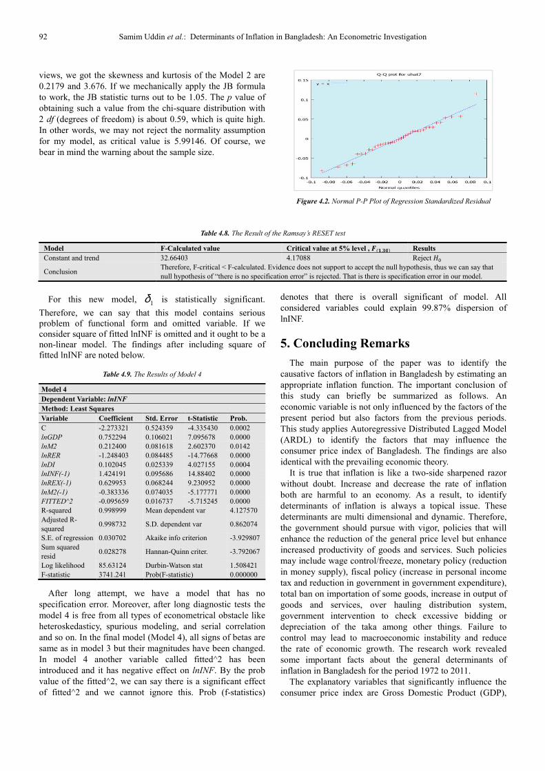
92 Samim Uddin et al.: Determinants of Inflation in Bangladesh: An Econometric Investigation
views, we got the skewness and kurtosis of the Model 2 are
0.2179 and 3.676. If we mechanically apply the JB formula
to work, the JB statistic turns out to be 1.05. The p value of
obtaining such a value from the chi-square distribution with
2 df (degrees of freedom) is about 0.59, which is quite high.
In other words, we may not reject the normality assumption
for my model, as critical value is 5.99146. Of course, we
bear in mind the warning about the sample size.
Figure 4.2. Normal P-P Plot of Regression Standardized Residual
Table 4.8. The Result of the Ramsay’s RESET test
Model F-Calculated value Critical value at 5% level , D)E.FG* Results
Constant and trend 32.66403 4.17088 Reject ?� Conclusion
Therefore, F-critical < F-calculated. Evidence does not support to accept the null hypothesis, thus we can say that
null hypothesis of “there is no specification error” is rejected. That is there is specification error in our model.
For this new model, is statistically significant.
Therefore, we can say that this model contains serious
problem of functional form and omitted variable. If we
consider square of fitted lnINF is omitted and it ought to be a
non-linear model. The findings after including square of
fitted lnINF are noted below.
Table 4.9. The Results of Model 4
Model 4
Dependent Variable: lnINF
Method: Least Squares
Variable Coefficient Std. Error t-Statistic Prob.
C -2.273321 0.524359 -4.335430 0.0002
lnGDP 0.752294 0.106021 7.095678 0.0000
lnM2 0.212400 0.081618 2.602370 0.0142
lnRER -1.248403 0.084485 -14.77668 0.0000
lnDI 0.102045 0.025339 4.027155 0.0004
lnINF(-1) 1.424191 0.095686 14.88402 0.0000
lnREX(-1) 0.629953 0.068244 9.230952 0.0000
lnM2(-1) -0.383336 0.074035 -5.177771 0.0000
FITTED^2 -0.095659 0.016737 -5.715245 0.0000
R-squared 0.998999 Mean dependent var 4.127570
Adjusted R-
squared 0.998732 S.D. dependent var 0.862074
S.E. of regression 0.030702 Akaike info criterion -3.929807
Sum squared
resid 0.028278 Hannan-Quinn criter. -3.792067
Log likelihood 85.63124 Durbin-Watson stat 1.508421
F-statistic 3741.241 Prob(F-statistic) 0.000000
After long attempt, we have a model that has no
specification error. Moreover, after long diagnostic tests the
model 4 is free from all types of econometrical obstacle like
heteroskedasticy, spurious modeling, and serial correlation
and so on. In the final model (Model 4), all signs of betas are
same as in model 3 but their magnitudes have been changed.
In model 4 another variable called fitted^2 has been
introduced and it has negative effect on lnINF. By the prob
value of the fitted^2, we can say there is a significant effect
of fitted^2 and we cannot ignore this. Prob (f-statistics)
denotes that there is overall significant of model. All
considered variables could explain 99.87% dispersion of
lnINF.
5. Concluding Remarks
The main purpose of the paper was to identify the
causative factors of inflation in Bangladesh by estimating an
appropriate inflation function. The important conclusion of
this study can briefly be summarized as follows. An
economic variable is not only influenced by the factors of the
present period but also factors from the previous periods.
This study applies Autoregressive Distributed Lagged Model
(ARDL) to identify the factors that may influence the
consumer price index of Bangladesh. The findings are also
identical with the prevailing economic theory.
It is true that inflation is like a two-side sharpened razor
without doubt. Increase and decrease the rate of inflation
both are harmful to an economy. As a result, to identify
determinants of inflation is always a topical issue. These
determinants are multi dimensional and dynamic. Therefore,
the government should pursue with vigor, policies that will
enhance the reduction of the general price level but enhance
increased productivity of goods and services. Such policies
may include wage control/freeze, monetary policy (reduction
in money supply), fiscal policy (increase in personal income
tax and reduction in government in government expenditure),
total ban on importation of some goods, increase in output of
goods and services, over hauling distribution system,
government intervention to check excessive bidding or
depreciation of the taka among other things. Failure to
control may lead to macroeconomic instability and reduce
the rate of economic growth. The research work revealed
some important facts about the general determinants of
inflation in Bangladesh for the period 1972 to 2011.
The explanatory variables that significantly influence the
consumer price index are Gross Domestic Product (GDP),
1δ
Journal of World Economic Research 2014; 3(6): 83-94 93
Money Supply (M2), Real Exchange Rate (RER) and Interest
Rate (IR) of the current year and Inflation Rate, Real
Exchange Rate and Money Supply of the previous year. Due
to lack of data and insignificance in Model, I had to ignore
some important variables as determinants of inflation like
Unemployment rate (necessary to explain the nature of
Phillip’s Curve in Bangladesh) remittance and Petroleum
Price (proxy of oil price). All considered variables except
real exchange rate help to increase inflation positively. These
explanatory variables combined to influence significantly the
rate of inflation in Bangladesh as much as 99% while the
stochastic error term (U1) captures 1%. At 5 percent level of
significance, they all influenced the rate of inflation during
the period.
Here sample size is only 39. Moreover, a specific
estimation method has been used. Lack of time prevented me
from taking other estimate methods. So the results obtain
hare could be improved in many ways. There is thus a scope
for further research on the topic.
6. Acknowledgements
We owe a great deal of gratitude to our honorable teacher
and research supervisor Professor Dr. Mohammad Abul
Hossain, Economics Department, University of Chittagong.
He offered us constant guidance and many insightful and
constructive observations throughout the study. His support,
encouragement and availability to discuss ideas and
problems have contributed much in completing this work. He
always kept us on task and pointing out us back to our
research paper objectives. We really appreciate for his
patience and high efficiency in guiding us in a proper way in
conducting this research. His friendly guidance and cooperation which is very rare inspired us to successfully
complete the whole work.
References
[1] Abidemi, O. I. and Maliq, A. A. A. (2010), “Analysis of Inflation and its Determinants in Nigeria”, Pakistan Journal of Social Sciences, Pakistan
[2] Adeyeye E. A. and Fakiyesi, T. O. (1980),“Productivity Prices and Incomes Board and Anti-inflationary Policy in Nigeria” The Nigerian Economy Under the Military, Nigerian Economic Society, Ibadan, Proceedings at the 1980 Annual Conference
[3] Ahmed N. (2009),“ Sources of inflation in Bangladesh”. Bangladesh Economic Association Conference Article No. 27.
[4] Akinnifesi (1984), “The deterministic scenario of Inflation in Nigeria”,Nigeria Journal of economics,Naigeria.
[5] Beckerman,P (1992)," The Economics of High Inflation", New York, NY: St. Martin’s Press.
[6] Begum,N (1991). “A Model of Inflation for Bangladesh,” Philippines Review of Economics and Business, Vol. 28, No. 1, pp. 100-117.
[7] Bera, A.K and Jarque, C,M (1981) “An Efficient Large-
Sample Test for Normality of Observations and Regression Residuals,” Australian National University Working Papers in Econometrics, Vol. 40 (1981), Canberra
[8] Bruno,M and Easterly, M (1995) “Inflation Crises and Long-Run Growth,” World Bank Policy Research Working Paper No. 1517 (1995)
[9] Dickey, D.A and Fuller,W.A (1979) “Distribution of the Estimators for Autoregressive Time Series with a Unit Root,” Journal of the American Statistical Association, Vol. 74 (1979), pp. 427-431.
[10] Dickey,D.A and Fuller,W.A (1981) “Likelihood Ratio Statistics for Autoregressive Time Series with a Unit Root”, Econometrica, Vol. 49 (1981), pp. 1057-1072.
[11] Engle,R and Granger, C(1987)“Co-integration and Error Correction: Representation, Estimation and Testing,” Econometrica, Vol. 55 (1987), pp. 1-87
[12] Engle,R and Yoo,B(1991) “Co-integrated Economic Time Series: An Overview with New Results,” in R. F. Engle and C. W. J. Granger, eds., Long-Run Economic Relationships, Oxford: Oxford University Press (1991), pp. 237-266.
[13] Faisal,F (2012), “Forecasting Bangladesh's Inflation Using Time Series ARIMA Models”, ; World Review of Business Research Vol. 2. No. 3. May. Pp. 100 – 117.
[14] Fashoyin,T. (1986) “Incomes and Inflation in Nigeria” Longman Publishers Ltd, New York
[15] Fatukasi,B (2005), “Determinants of Inflation in Nigeria: An Empirical Analysis International” Journal of Humanities and Social Science Vol. 1 No. 18 www.ijhssnet.com 262.
[16] Friedman,M and Schwartz,J (1963) "A Monetary History of the United States, 1867-1960", Princeton, The Princeton University Press, 1963.
[17] Gavin,T & Kevin,K.L. (September 2006), “Forecasting Inflation and Output: Comparing Data-Rich Models with Simple Rules”, Research Division, Federal Reserve Bank of St. Louis, Working Paper Series
[18] Godfrey,G (1978) “Testing Against General Autoregressive and Moving Average Error Models When the Regressors Include Lagged Dependent Variables,” Econometrica, Vol. 46 (1978), pp. 1293-1301.
[19] Godfrey,G. (1978) “Testing for Higher Order Serial Correlation in Regression Equations When the Regressors Include Lagged Dependent Variables”, Econometrica, Vol. 46 (1978), pp.1303-1310.
[20] Greene,H (2003) “Econometric Analysis”. 5th
Ed. New Jersey: Prentice-Hall (2003).
[21] Gujarati,N (2003), “Basic Econometrics”, 4th ed., McGraw-Hill. Chapter 11.
[22] Hafer,W and Hein,S (January 1990), “Forecasting Inflation Using Interest Rate and Time-Series Models: Some International Evidence”, The Journal of Business, Vol.63, No.1, 1-17.
[23] Hendry,F (1990) Productive Failure Econometric Modeling in Macroeconomics: The Transmission Demand for Money,” in Economic Modeling: Current Issues and Problems in Macroeconomic Modeling in the UK and the USA, (ed.), London:
94 Samim Uddin et al.: Determinants of Inflation in Bangladesh: An Econometric Investigation
[24] Hendry,F. (1995), “Dynamic Econometrics”, London: Oxford University Press pp. 577
[25] Hossain,A (2002), “Exchange Rate Response of Inflation in Bangladesh”,
[26] Humphrey,T (1998), "Historical Origins of the Cost-Push Fallacy", Richmond, Federal Reserve Bank of Richmond Economic Quarterly, 84 (3), P 53–74,
[27] Jarque,M and Bera.A (1980) “Efficient Tests for Normality, Homoscedasticity and Serial Independence of Regression Residuals,” Economics Letters, Vol. 6, pp. 255-259.
[28] Johansen,S. (1988), “Statistical Analysis of Co-integration Vectors,” Journal of Economic Dynamics and Control, Vol. 12 (1988), pp. 231-254.
[29] Johansen,S. and Juselius,K. (1990) “Maximum Likelihood Estimation and Inference on Co-integration with the Application to the Demand for Money,” Oxford Bulletin of Economics and Statistics, Vol. 52, (pp. 169-210.
[30] Judson and Orphanides (1999) “Non-linear Effects of Inflation on Economic Growth‟, IMF Working Staff Papers, Vol. 43(1), pp.199–215
[31] Kabundi,A (2012), “Dynamics of Inflation in Uganda”, African Development Bank Group, Working Paper No. 152
[32] Kazi,M, Arif1,M & Munshi,A (2012), “ Determinants of Inflation in Bangladesh: An Empirical Investigation”, Journal of Economics and Sustainable Development Vol.3, No.12, 2012. www.iiste.org ISSN 2222-1700 (Paper) ISSN 2222-2855 (Online).
[33] Kirkpatrick,C and Nixon,F (1976) " The Origins of Inflation in Less Developed Countries": A Selective Survey, Manchester, The Manchester University Press, 1976.
[34] Kozo & Ueda (2009) “Determinants of Households’ Inflation Expectations”, Institution for Monetary and Economic Studies Bank of Japan, Discussion Paper No. 2009-E-8
[35] Kwiatkowski,D et.al (1992), “Testing the Null Hypothesis of Stationarity Against the Alternative of a Unit Root,” Journal of Econometrics, Vol. 54 (1992), pp. 159-178.
[36] Lipsey, R. ,Steiner,P and Purvis,D. (1982). “Economics”, 7th Edition, New York: Harper Collins Pub. Inc.
[37] MacKinnon,J. (1991) “Critical Values for Co-integration Tests,” In R. F. Engel and C. W. J. Granger, eds., Long Run Economic Relationships: Readings in Co-integration, Oxford: Oxford University Press
[38] Majumdar,M (2006) “Inflation in Bangladesh: Supply Side Perspectives”. Bangladesh Bank Policy, Note Series: PN 0705.
[39] Mallik,G and Chowdhury,A (2001), “Inflation and Economic Growth: Evidence from South Asian Countries,” Asian Pacific Development Journal, Vol. 8, No.1), pp. 123-135.
[40] McCallum,T (1987) “Inflation: Theory and Evidence", New York, TheAmerican National Bureau of Economic Research, Working Paper No. 2312, 1987.
[41] Mortaza,G and Rahman,H (2008), “Transmission of International Commodity Prices to Domestic Prices in Bangladesh”, Working Paper Series: WP 0807 ; Policy Analysis Unit (PAU), Bangladesh Bank.
[42] Osmani,S (2007). “Interpreting Recent Inflationary Trends in Bangladesh and Policy Options”, Presented at a dialogue, Centre for Policy Dialogue (CPD), September 2007.
[43] Patterson,K (2002) “ An Introduction to Applied Econometrics: A Time Series Approach”, New York: Palgrave (2002).
[44] Phillips,C and Perron, P (1998) “Testing for a Unit Root in Time Series Regression,” Biometrika, Vol. 32, pp. 301-318.
[45] Raihan,S and Fatema,K. (2007) “A review of the current hypotheses on inflation In Bangladesh”. Working Paper (02-07), Bangladesh.
[46] Ramakrishnan,U.andVamvakidis,A (June 2002),“Forecasting Inflation in Indonesia”, IMF Working Paper No. 02/111.
[47] Ramsey,J (1969) “Test for Specification Errors in Classical Linear Least Square Regression Analysis,” Journal of the Royal Statistical Society B (1969), pp. 350-371.
[48] Ramsey,J (1970)“Models, Specification Error and Inference: A Discussion of Some Problems in Econometric Methodology”, Bulletin of the Oxford Institute of Economics and Statistics, Vol. 32 (1970), pp. 301-318.
[49] Ratnasiri, H (2006), “The Main Determinants of Inflation in Sri Lanka :A VAR based Analysis”, Central Bank of Sri Lanka, Staff Studies – Volume 39 N0 1 & 2.
[50] Ricardo,D (1817) “Principles of Political Economy and Taxation, London”, Murrary Publication, 1817
[51] Sarel,M (1995) “Nonlinear Effects of Inflation on Economic Growth,” IMF Working Paper WP/95/56, Washington (May 1995).
[52] Shamim,A and Mortaza,G. (2005) “Inflation and Economic Growth in Bangladesh: 1981-2005” Working Paper Series: WP 0604 Policy Analysis Unit (PAU) Research Department, Bangladesh Bank
[53] Sun,T (May 2004), “Forecasting Thailand’s Core Inflation”, IMF Working Paper, WP/04/90
[54] Taslim,A (1980) Inflation in Bangladesh : A Re examination of the Structuralist Monetarist controversy. The Bangladesh development studies vol X No 1
[55] Temple,J (2000), “Inflation and Growth: Stories Short and Tall‟, Journal of Economic Surveys, Vol. 14, No. 4, pp. 395–426.
[56] Totonchi,J (2011) “Macroeconomic Theories of Inflation”, International Conference on Economics and Finance Research, IPEDR vol.4 (2011) © (2011) IACSIT Press, Singapore
[57] Ubide,A (1997), “Determinants of inflation in Mozambique”, International Monetary Fund, African Department