Forecasting

Including an Introduction to Forecasting using the SAP R/3 System

by

James D. Blocher

Vincent A. Mabert Ashok K. Soni

Munirpallam A. Venkataramanan

Indiana University Kelley School of Business

February 2004

Introduction and Overview ...................................................................... 2 Forecasting and Supply Chain Planning................................................. 2

Forecasting Practice .................................................................................................... 3 Supply Chain Improvements for Better Forecasts ...................................................... 4 Forecasting Methods................................................................................................... 5

Qualitative Input ..................................................................................................... 5 Quantitative Input ................................................................................................... 6

Simple Time Series Models....................................................................... 7 Projection .................................................................................................................... 7 Simple Moving Average (MA)................................................................................... 7 Weighted Moving Average (WMA)........................................................................... 8 Basic Exponential Smoothing (BES).......................................................................... 8 Simple Time Series Example...................................................................................... 9

Forecast Accuracy ................................................................................... 10 Average Error and Bias............................................................................................. 11 Mean Absolute Deviation ......................................................................................... 12 Mean Absolute Percentage Error .............................................................................. 12 Mean Squared Error.................................................................................................. 12 Tracking Signal......................................................................................................... 12 Forecast Error Example ............................................................................................ 13 Smoothed Error Measures......................................................................................... 13 Errors as an Estimate of Forecast Uncertainty.......................................................... 14 A “Reaction-to-Error” Interpretation of Exponential Smoothing............................. 15

Multi-Factor Time Series Methods........................................................ 15 Trend-Enhanced Forecasting Models ....................................................................... 16

Exponential Smoothing Updates – Holt’s Model ................................................. 16 Trend- and Seasonality-Enhanced Forecast Models................................................. 17

Exponential Smoothing Updates – Winters’ Model ............................................. 17 Model Initiation and Forecasting .............................................................................. 17

Holt’s Additive Trend Model Example ................................................................ 18 Winters’ Additive Trend, Multiplicative Seasonality Model Example ................ 20

Deseasonalizing Demand.................................................................................. 20 Determining the Initial Forecasting Factors ..................................................... 22 Forecasting with Winters’ Model ..................................................................... 23

Forecasting References ........................................................................... 26 Time Series Forecasting Problems......................................................... 27 Forecasting with SAP R/3....................................................................... 29

Loading Historical Data............................................................................................ 29 Forecasting With SAP R/3: Steps and Input Requirements...................................... 33

User Selection Approach to Forecasting............................................................... 33 System Selection Approach to Forecasting .......................................................... 36

Summary…………………………………………………………………………40 Creating Part Numbers…… ……………………………………… ……………...41 Glow-Bright Corporation Case.............................................................. 44

1

Introduction and Overview A key part of supply chain planning involves demand planning and the associated demand forecasting process. The focus here is on the various issues involved in forecasting and their use in the SAP R/3 system. The objectives of this document are to

• highlight the need for forecasting to manage the supply chain, • provide statistical time series models for short-term forecasting, • review forecasting performance metrics and tracking procedures, and • illustrate how forecasting is done in the SAP R/3 system.

To help develop an understanding of the statistical methods, some example problems are included. It should be noted that this module does not cover regression methods as this topic is covered in depth in many other places.

Forecasting and Supply Chain Planning Supply chain planning, to a large degree, starts with forecasting. Matching supply and demand is an important goal for most firms and is at the heart of operational planning. It is also of significant importance as the overly optimistic Cisco found in 2001 when it took a $2.2 Billion inventory write-down because of their ability to “forecast demand with near-scientific precision” 1. Since most production systems can’t respond to consumer demand instantaneously, some estimate, or forecast, of future demand is required so that the efficient and effective operational plans can be made. Plant, process, and labor capacity are all set based on the forecasts of future demand. Capacity planning and facility decisions would be based primarily on longer term, aggregate forecasts. However, forecasts are also needed to plan proper inventory levels, which in general, tend to require shorter-term forecasts at a disaggregated level since specific components, parts, and end-items must be stocked for immediate consumer demand. Forecasts affect most functional areas of the firm and are the starting point for resource allocation decisions. For example, manufacturing must plan production on a day to day basis to meet customer orders, while purchasing needs to know how to align supplier deliveries with the production schedules. Finance needs to understand the forecasts so that the proper levels of investment can be made in plant, equipment, and inventory and so that budgets can be constructed to better manage the business. The marketing function needs to know how to allocate resources for various product groups and marketing campaigns. Forecasts also determine the labor requirements required by the firm so that the human resources function can make proper hiring and training decisions when demand is expected to grow. 1 “Cisco’s Comeback”, Business Week Online, November 24, 2003

2

Forecasting Practice Forecasts are always wrong, but some are “more wrong” than others. Forecasting the demand for innovative products, fashion goods, and the like is generally more difficult than forecasting demand for more “commodity-like” products that are sold on a daily basis. Aggregate forecasts of a group of similar products are generally more accurate than individual forecasts of the individual products that make up the group. Finally, the longer the forecast into the future, the less reliable the forecast will be. Forecasting practice is based on a mix of qualitative and quantitative methods. When planning occurs for innovative products, little demand data are available for the product of interest and the degree to which like product demand data are similar is unknown. Thus a large amount of judgment is needed by experts who can use their industry expertise to predict demand. These experts, though, will undoubtedly use historical demand data, even if not directly, in their judgment. Commodity-like products that are sold everyday, on the other hand, are much more suitable for quantitative models and need very little judgment to forecast demand. Still, when knowledge of certain events leads one to believe that future demand might not track historical trends, some judgment may be warranted to make adjustments in the models which use past data. In this case, a heavy reliance on past data with adjustments based on expert judgment should be the method used for forecasting. Forecasting should be done primarily for end-item demand. In manufacturing situations, this means there is no real need for forecasting component parts which make up the final item. When production quantities for the end item have been determined, component demand can be computed based on the production plan of the end item and knowledge of the bill of materials (BOM). Aggregating forecasts across multiple items reduces forecasting errors. A clothing store, for instance, might be able to estimate within a pretty narrow range what the demand will be for men’s dress shirts. But when that store tries to estimate the demand for individual styles, colors, and sizes of shirts, the accuracy of their forecasts will be considerably worse. Firms handle this kind of forecasting problem usually in one of three ways; they either forecast from the bottom up, from the top down, or they start in the middle and work both up and down. The “top down” forecast essentially estimates total sales demand and then divides those sales dollars level by level until the stock keeping unit (SKU) is reached. The “bottom up” method, as one might expect, starts with forecasts at the SKU level and then aggregates those demand estimates level by level to reach a company–level forecast. Another method, one might call the “in-between” method, starts forecasts at the category level (like men’s dress shirts), and then works up to determine store sales and works down to divide up the forecast into styles, colors and SKUs. The use of management time to make forecasts is relatively expensive when compared to the cost of using statistical forecasting models, and the difference between the costs of these two methods has been increasing in recent years due to the automated acquisition of data from point of sale systems and computer power in general. There can be no

3

substitute for human input in the forecasting process; however, human input can be expensive. In addition, research indicates that for some everyday commodity-type items, simple statistical models work well and in fact work better when not massaged by managers. Still, some managers believe that spending time to make forecasts perfect will solve most of their supply chain problems. There are times when managerial input is needed, but there comes a point where it is better to understand the inaccuracy in the forecast and plan accordingly. Once a good forecasting process (procedures, techniques, models and management oversight) has been put in place, continual refinement has little value and can even hurt the forecasting process.

Supply Chain Improvements for Better Forecasts Since forecasts are never accurate, two common solutions are often proposed to “fix” forecast errors. The first is to reduce the lead time to react sooner to changes. This is a good partial solution, but reducing lead times is not always easy to do and is often expensive. In addition, shortening the lead time, in many cases, just moves the problems from one part of the supply chain to another. The second is to “make to order” so that inventory doesn’t need to be produced in advance of demand. This solution is also good, but like shortening the lead time, tends to shift demand to the next level of the supply chain. Furthermore, producing to order still requires forecasts, to be able to keep the right quantities of raw material on hand. So while these ideas help improve certain aspects of the forecasting problem, they do not eliminate the need for some kind of forecasting methods. A more recent proposal to fix forecast errors is to use collaboration. The idea is that if different parts of the supply chain collaborate on a common forecast and everyone plans based on that single forecast; then there is little need for one part of the chain to hedge based on the uncertainty of what is done in other parts of the chain. Intra-firm collaboration, you would think, would be common place – seems that a little common sense would dictate that everyone in a firm come together with a common set of forecast figures. But this is rarely the case. Marketing has a set of forecasts, so too does operations. Sales has their forecast and it’s possible that for budgeting purposes Finance uses still another. The advancement of enterprise resource planning (ERP) systems is helping ensure that there is only one forecast, based upon the principles of a single data repository used by all areas of the enterprise. Once functional areas within a firm agree on a common forecast, the next step is for inter-firm agreement. This type of collaboration is tougher, but many believe it is an essential step in the continual improvement of the supply chain. The collaborative planning, forecasting, and replenishment (CPFR) multi-industry initiative is aimed at providing this kind of integrative forecast between so-called “trading partners” – different levels in the supply chain. Supply chain advanced planning system (APS) models and software packages are designed to connect the various supply chain players so that this collaboration can be completed successfully. But there is much to do in this area to end the second guessing that is so prevalent today.

4

Forecasting Methods Forecasting is based on a mix of qualitative and quantitative inputs. The type of product and that product’s impact on supply chain costs determine how much human input is used and how sophisticated the forecasting model should be.

Qualitative Input Human judgment can be captured in a number of ways. Three common approaches include an Individual Market Expert, Group Consensus, and the Delphi Method. All of these are sometimes referred to as Expert Opinion methodologies since they require people with some knowledge of the products and markets developing forecast estimates for planning needs. Individual Market Experts can be hired to watch for industry trends, perhaps even by geographic area, and might even work with sales people to estimate future demand for products. Individuals, though, have biases that they may not be aware of and there is a limit to how much information one person can obtain. To overcome this, even though it can be considerably more expensive, is to use groups of experts. Group Consensus involves bringing together a team of experts, hopefully from different functional areas, to reach consensus on future forecasts for a product or a group of products. Group Consensus forecasts tend to bring together different factions of the company so that everyone tends to “buy-in” the final numbers. The group gets to make sure that over-zealous managers don’t over-forecast just to try to meet firm expectations for growth. The group also gets to make sure someone doesn’t play conservative and under-forecast because that person thinks it is less risky to “low-ball” the forecast. But, building consensus has its pitfalls as well. When people from different ranks in the firm come together, there can be a tendency for low-ranking personnel to at some point acquiesce to the higher-ranking managers in the group. This defeats the point of coming to a consensus agreement and can be a real problem with certain personalities. One way to overcome this issue is to come to an anonymous consensus by using something known as the Delphi Method. The Delphi Method requires one person to administer and coordinate the process and poll the team members (respondents) through a series of sequential questionnaires. While the team members need to be people who have some expertise in the area of interest to the forecast, the administrator only needs to have some knowledge of how to coordinate the effort without unduly influencing the results. The questionnaires that are sent to the members involve not only estimates of demand, but they are aimed at determining how the member is reaching that estimate. Once everyone has returned the questionnaires, the administrator must summarize the results and send a summary report to all of the members, but, with the identity of who made which forecast hidden from the team. Along with the summary is another questionnaire which in some ways builds off of the previous forecasts and assumptions used in those forecasts. This process of questionnaire, summary, questionnaire, summary continues until the participants reach some consensus on the forecast. Obviously this method can be both time consuming and

5

rather expensive to administer but it can lead to good forecasts and in addition, it establishes over time the important inputs to the process. Three rounds seems to be a good compromise between forecast quality and the cost and effort involved.

Quantitative Input Quantitative analysis typically involves two approaches: causal models and time-series methods. Causal models establish a quantitative link between some observable or known variable (like advertising expenditures) with the demand for some product. Time series analysis involves looking at historical demand for a product to forecast future demand. The most common types of Causal Models are regression analysis and econometric models. While regression models can be quite involved, simple linear regression is often used, whereby a straight line of the form Y = mX + b is used to describe the relationship between the dependent variable Y and the independent variable X. The line is fit through a set of points such that the squared distance from the line is minimized, thus a “least square” fit. Econometric models are usually some form of multivariate regression model where the independent variables (many Xs) represent factors like disposable income and industrial output from the economy. The mathematical details of regression are not covered here. There are a number of different kinds of Time Series Models, most of which work on the assumption that historical demand can be “smoothed” by averaging and that past demand “patterns” will continue to occur in the future. Simple time series analysis includes models such as the Weighted Moving Average and Basic Exponential Smoothing. More complex time series methods include factors for trends, seasonal patterns, and economic cycles. The remainder of this reading focuses on these time series models.

6

Simple Time Series Models Some of the most popular forecasting methods, especially in software packages, are commonly referred to as time series models. These models make use of past data to predict future demand. This type of forecasting method is especially relevant for items which are continuously ordered as these methods can be “automated” in computer information systems to a large degree. The models assume that each observed demand data point is comprised of some systematic component and some random component. The time series model is designed to predict the systematic component but not the random component. The idea is similar to the logic of quality control charts in that you don’t try to react to the process variability as long as it is within the control limits. Reacting (or changing the forecast model) because of errors that are random is only likely to increase the error in future forecasts. What is needed is to try to predict the range or variation of this random error. Models can be designed for just about any type of systematic change in demand, but there is real danger in trying to predict the random component.

Projection The easiest time series method simply projects future demand based on the last period’s demand. The forecast for the next period t+1, Ft+1, is simply a projection of this period t demand, Dt tt DF =+1 (1) This method, although easy to use, doesn’t make use of data that is easily available to most managers; thus, using more of the historical data should improve the forecast. Averages of past demand might be more useful and are discussed next.

Simple Moving Average (MA) The simple moving average forecast makes use of more of the historical demand data than just the last period’s demand. An n-period moving average uses the last n periods of demand as a forecast for next periods demand:

n

DDDDF ntttt

t121

1... +−−−

+

++++= (2)

This forecast model is most useful where the demand level is fairly constant over time. The model then makes simple adjustments to this average level rather than assuming that the level is forever constant. Its advantage over the projection model is that by averaging, the forecast won’t tend to fluctuate as much. The average of the previous n periods can be viewed as the estimate of the average “level” of demand as of period t. Thus, one could define the level, Lt, as

7

n

DDDDL ntttt

t121 ... +−−− ++++

= (3)

and thus the forecast, Ft+1, is just the last estimate of the level of demand. tt LF =+1 (4) This forecast is no different than the direct forecast given above in Equation 2, but the interpretation allows for an easier presentation of the more advanced forecasting models to come.

Weighted Moving Average (WMA) One shortcoming of the simple moving average is the equal weighting of data. For instance, a 5-period moving average weights each of the past 5 demand observations the same – each has a 20% impact on the forecast. This runs counter to ones intuition that the most recent data is the most relevant. Thus, the weighted moving average allows for more emphasis to be placed on the most recent data. This forecast is:

121

1122111 ...

...

+−−−

+−+−−−−−+ ++++

++++==

ntttt

ntnttttttttt wwww

DwDwDwDwLF (5)

where wt is the weight applied to the demand incurred in period t, wt-1 is the weight given to that of period t-1, and so on

Intuitively, the expectation would be that the more recent demand data should be weighted more heavily than older data; so, generally, one would expect the weights to follow the relationship wt ≥ wt-1 ≥ wt-2 ≥ … .

Basic Exponential Smoothing (BES) Nice properties of a weighted moving average would be one where the weights not only decrease as older and older data are used, but one where the differences between the weights are “smooth”. Obviously the desire would be for the weight on the most recent data to be the largest. The weights should then get progressively smaller the more periods one considers into the past. The exponentially decreasing weights of the basic exponential smoothing forecast fit this bill nicely. The forecast equation is given by:

tttt FDLF )1(1 αα −+==+ (6)

where α is a smoothing parameter between 0 and 1. To show that this forecast is in fact a weighted average forecast, it is instructive to look at the algebraic expansion of this model. Since 11 )1( −− −+= ttt FDF αα

8

])1()[1( 111 −−+ −+−+= tttt FDDF αααα

12

11 )1()1( −−+ −+−+= tttt FDDF αααα

This too can be expanded since 221 )1( −−− −+= ttt FDF αα

])1([)1()1( 222

11 −−−+ −+−+−+= ttttt FDDDF αααααα

23

22

11 )1()1()1( −−−+ −+−+−+= ttttt FDDDF αααααα Continuing this expansion, the model can be written as:

...)1()1()1( 33

22

11 +−+−+−+= −−−+ ttttt DDDDF ααααααα (7) Thus, the exponential smoothing model is actually a weighted moving average model with special weights. These weights get continuously smaller as they are applied to periods farther away from the current period. With some algebra, it can be shown that these weights sum to one (8) 1...)1()1()1( 32 =+−+−+−+ ααααααα

Even though these weights have nice properties, it is not necessary to keep track of each of the weights. In addition, a system running the model does not need to store the historical data or does it need to compute anything based on old data. The only thing that is needed is the smoothing factor α, last period’s demand, and last period’s forecast. The nice thing about the model is that all past demand data is effectively “stored” in the last period’s forecast.

0

0.05

0.1

0.15

0.2

0.25

0.3

0.35

t t-3 t-7

Time Period

Wei

ght

t-5 t-9t-1 t-6t-4 t-10t-8t-2

Weights vs. Time Period: α=0.3

0

0.05

0.1

0.15

0.2

0.25

0.3

0.35

t t-3 t-7

Time Period

Wei

ght

t-5 t-9t-1 t-6t-4 t-10t-8t-2

Weights vs. Time Period: α=0.3

Figure 1: Effective Weights for BES

Simple Time Series Example The models presented above are now illustrated using a simple data set. Eight periods of demand data for a product are given for January through August in Table 1. The period designation in the table is the same as referred to in the models.

Table 1: Seasonal Estimates and Initial Seasonal Factors

9

The firm wishes to forecast demand for September (period t+1). These calculations are presented below. Simple Projection

Ft+1 = Dt ; Ft+1 = 48.

Simple Moving Average (using 4 periods)

474

55474148... 1211 =

+++=

++++= +−−−

+ nDDDD

F nttttt

Weighted Moving Average (using 4 periods with wt =0.4, wt-1 =0.3 wt-2 = 0.2, wt-3 = 0.1)

1.461

)55(1.0)47(2.0)41(3.0)48(4.0...

...

121

1122111

=+++

=

++++++++

=+−−−

+−+−−−−−+

ntttt

ntntttttttt wwww

DwDwDwDwF

Basic Exponential Smoothing (with α=0.2) To employ BES, the firm uses the past demand data to train the model. To do this training, forecasts need to be computed for each period for which there is demand data. Table 2 shows the forecast for September of 46.4 and the computations needed to obtain that forecast using the exponential model. By letting the forecasting model run through past data, a sort of smoothing takes place so that future forecasts are based on good weights. This training with past data also allows the forecaster to measure the forecast errors based on the model assuming that it was actually used in the past to make forecasts.

Table 2: BES Calculations

Forecast Accuracy Since forecasts are always wrong, an estimate of the inaccuracy of the forecast can be just as helpful as the forecast of the expected demand. So a good forecast needs to include a mean and an estimate of how the forecast will vary around the mean. This measure helps us understand the risk of the forecast and allows us to make decisions allowing for

10

variability that is present. Forecasting involves estimating more than the expected demand – it involves trying to estimate the uncertainty as well. To ascertain how well a forecast model is working, actual past demand information is compared to the forecast for that period. These forecast errors, not only tell a firm how well their forecast system is working, they also provide information about how much risk there is in the forecast by helping a manager understand the inherent variation in the demand. An estimate of the future forecast variation is based, at least in part, on the variation of past forecasts. Many times this estimate of the accuracy of a forecast is consistent over time and can be used to establish upper and lower estimates of expected demand. The forecast error for period t is defined as2 ttt DFE −= (9) Several different error metrics are used in practice, with different strengths. They are based on various functional sums of these individual period-t forecast errors as explained below.

Average Error and Bias The simple average error over n periods is

∑=

=n

iin E

nAE

1

1 (10)

but one would expect that a good forecast would be such that the expected value of AEn is zero since positive and negative deviations should cancel each other out. In fact, it would be good to know the value of AEn, since it indicates how good the forecast is tracking the actual demand. A similar more common measure, known as the bias, is usually used to track this “systematic” error and is given as:

(11) ∑=

=n

iin Ebias

1

Managers are interested in forecasts with no bias. When a bias exists, it is likely that the wrong functional forecast model is being used. Systematic bias should, theoretically, be something that can be eliminated by introducing some factor in the model to remove it from the forecast. Thus, this simple error measure can be one of the most important in determining if the correct forecasting model is being used.

2 Some authors define error as Et = Dt – Ft. This definition requires the user to be aware of how to interpret the positive or negative sign of the errors.

11

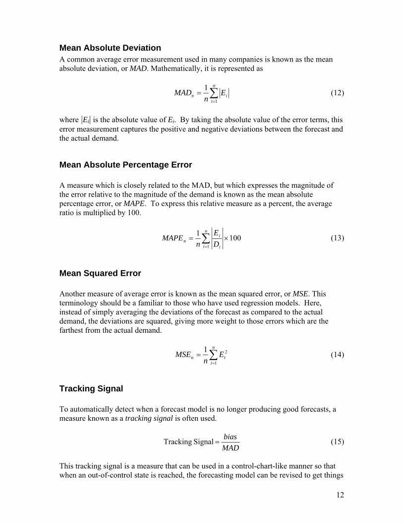
Mean Absolute Deviation A common average error measurement used in many companies is known as the mean absolute deviation, or MAD. Mathematically, it is represented as

∑=

=n

iin E

nMAD

1

1 (12)

where |Ei| is the absolute value of Ei. By taking the absolute value of the error terms, this error measurement captures the positive and negative deviations between the forecast and the actual demand.

Mean Absolute Percentage Error A measure which is closely related to the MAD, but which expresses the magnitude of the error relative to the magnitude of the demand is known as the mean absolute percentage error, or MAPE. To express this relative measure as a percent, the average ratio is multiplied by 100.

10011

×= ∑=

n

i i

in D

En

MAPE (13)

Mean Squared Error Another measure of average error is known as the mean squared error, or MSE. This terminology should be a familiar to those who have used regression models. Here, instead of simply averaging the deviations of the forecast as compared to the actual demand, the deviations are squared, giving more weight to those errors which are the farthest from the actual demand.

∑=

=n

itn E

nMSE

1

21 (14)

Tracking Signal To automatically detect when a forecast model is no longer producing good forecasts, a measure known as a tracking signal is often used.

MADbias Signal Tracking = (15)

This tracking signal is a measure that can be used in a control-chart-like manner so that when an out-of-control state is reached, the forecasting model can be revised to get things

12

back in control. By dividing the bias by the MAD, the control limits for this “unit-less” measure are the same for every product being forecast and therefore separate control limits need not be kept for each product. Instead, a common rule of thumb is when the tracking signal reaches a value of positive or negative “6”, it is time to investigate the forecasting model.

Forecast Error Example To illustrate some of these error measures, the demand data and forecasts from the example problem presented in Table 2 will be used. The demand is compared to the forecast for each period with the resulting errors give in Table 3. This provides values for the error, Ei, for each period t from January through August. The last two columns of this table show the forecast error and the squared forecast error for each of the periods of interest. Table 3: Seasonal Factors

9.20.23.63.08.52.03.54.30.2 =−++−++−== ∑=

−

Aug

JaniiAugJan Ebias

2.38

3.258

0.23.63.08.52.03.54.30.21==

+++++++== ∑

=−

Aug

JaniiAugJan E

nMAD

1.158

8.1208

0.23.63.08.52.03.54.30.21 222222222 ==

+++++++== ∑

=−

Aug

JanitAugJan E

nMSE

9.02.39.2 Aug) of (as Signal Tracking ===

MADbias

Smoothed Error Measures Since errors are sometimes used to estimate demand variation, it is useful to think about an exponentially smoothed MAD so that recent errors are weighted more heavily. Smoothing the error is very similar to the basic exponential forecasting technique. Thus, each period a new MAD is computed as ( ) 11 −−+= ttt MADEMAD δδ (16)

where δ is a smoothing parameter between 0 and 1.

13

Errors as an Estimate of Forecast Uncertainty Forecasts usually consist of just a mean; but, an estimate of the standard deviation of the uncertainty of future forecasts can be just as important. The firm needs to know how much risk is in the forecast. For example, good inventory models need some measure of demand uncertainty, or more accurately, forecast uncertainty, to determine the proper levels of safety stock inventory. Inventory models which use past demand variation are likely calling for too much safety stock; a good forecast may be able to predict some of this uncertainty and the safety stock is only needed for the unpredictable part. Two common measures of the standard deviation of the forecast errors are presented next. One of these is based on the absolute deviation. When forecast errors are normally distributed and have no bias, the MAD can be used to estimate the standard deviation, MAD25.1=σ . (17) The other measure is based on the direct estimate of mean squared deviation statistic and is given as

1

)(1

2

−

−=∑=

n

EEn

tt

σ . (18)

14

A “Reaction-to-Error” Interpretation of Exponential Smoothing Since , the forecast using the exponential smoothing model can be rewritten as

ttt DEF +=

tttt FEFF )1()(1 αα −+−=+ (19)

which, with a little algebra, can be rewritten as ttt EFF α−=+1 (20) Thus, each new forecast can be interpreted as the past forecast adjusted by some percentage of the last forecast’s error. When the forecast error is positive, the forecast overestimated the demand; therefore, the next forecast needs to be reduced. The smoothing parameter α determines by how much the forecast should be modified.

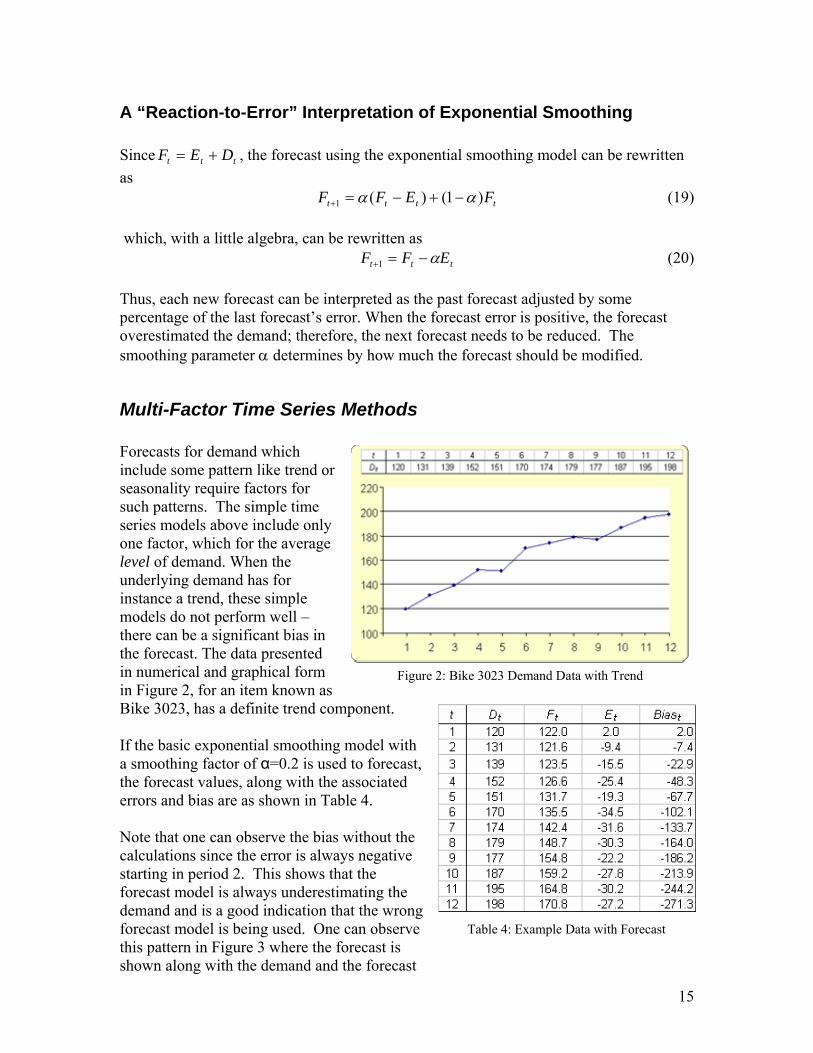
Multi-Factor Time Series Methods Forecasts for demand which include some pattern like trend or seasonality require factors for such patterns. The simple time series models above include only one factor, which for the average level of demand. When the underlying demand has for instance a trend, these simple models do not perform well – there can be a significant bias in the forecast. The data presented in numerical and graphical form in Figure 2, for an item known as Bike 3023, has a definite trend component.

Figure 2: Bike 3023 Demand Data with Trend

If the basic exponential smoothing model with a smoothing factor of α=0.2 is used to forecast, the forecast values, along with the associated errors and bias are as shown in Table 4. Note that one can observe the bias without the calculations since the error is always negative starting in period 2. This shows that the forecast model is always underestimating the demand and is a good indication that the wrong forecast model is being used. One can observe this pattern in Figure 3 where the forecast is shown along with the demand and the forecast

Table 4: Example Data with Forecast

15

is always under forecasting or lagging the demand. Therefore, demand that has some pattern like a trend or seasonality should be forecast with a model that contains the adjustment factor for the pattern.

Trend-Enhanced Forecasting Models

Figure 3: Demand and Forecast Information

The functional form of a model which forecasts demand with a trend parameter requires two components, a level component, L, and a trend component, T. When Tt is used to represent an estimate of the trend as of period t, the model for forecasting one period into the future is ttt TLF +=+1 (21) The additive trend adjustment is one of the most commonly used and is sometimes referred to as Holt’s Model. To forecast the ‘rth’ period into the future, the model is ttrt rTLF +=+ (22)

Exponential Smoothing Updates – Holt’s Model Each period when more information becomes available, the level and trend factors can be updated. This is done with equations very similar to the equations for the basic exponential smoothing model presented earlier. For the basic exponential smoothing model, a smoothing parameter α was used to determine how much of the new demand information should be included in the level factor. Since there are now two factors, level and trend, a second smoothing parameter β is needed for determining the amount of smoothing to be done on the trend factor. Values for β are between 0 and 1. The updating equations for each factor for the case of additive trend (Holt’s model) are ))(1( 11 −− +−+= tttt TLDL αα (23) 11 )1()( −− −+−= tttt TLLT ββ (24)

16

Trend- and Seasonality-Enhanced Forecast Models When both trend and seasonal factors are present, along with the average level factor, the forecast equation is a combination of the three factors. The most common model and one known as Winters’ Model, assumes an additive trend factor and a multiplicative seasonality factor. This model for forecasting one period into the future is 11 )( ++ ×+= tttt STLF (25) The factor for seasonality, St+r , is the seasonal factor for the period t+r, r periods in the future. Note that there is a seasonal factor for every “season”. If the forecast is quarterly, then there are four seasonal factors. If the forecast is done monthly or weekly, then there are twelve or 52 seasonal factors respectively. In some short-term forecasting situations, where demand varies by the day of the week, there could be a seasonal factor for each day of the week, or seven factors. For forecasting r periods into the future, the form is rtttrt SrTLF ++ ×+= )( (26)

Exponential Smoothing Updates – Winters’ Model Just as was done for the additive trend model (Holt’s model), the factors for additive trend and multiplicative seasonality (Winters’ model) can be updated as new information becomes available. In addition, since there are now three factors, a third smoothing parameter γ is needed for seasonality. The updating equations are then

))(1( 11 −− +−+= ttt

tt TL

SD

L αα (27)

11 )1()( −− −+−= tttt TLLT ββ (28)

tt

tpt S

LDS )1( γγ −+=+ (29)

where p is the number of “seasons” (e.g., p=12 for monthly data with a yearly cycle).

Model Initiation and Forecasting Just as was the case for the basic exponential smoothing model, it is important to find good initial starting factors and then “train” the model. But for the multi-factor models, this is a little more involved. Two sets of example data are used below to illustrate this initiation on Holt’s and Winters’ models.

17

Holt’s Additive Trend Model Example Managers at Dynostasio want to set up forecasting models for their most popular products. The demand for one of their products which has seen phenomenal growth since its introduction is shown in Table 5. This product has been on the market since January o2003 and thus the there is demand data for this product for eleven periods through November of 2003. An analyst for the firm has decided to use Holt’s Model to forecast future demand and in particular come up with an estimate of demand for December of 2003.

f

Since the model assumes an additive trend, a straight line can be fit to the data to estimate the initial level factor (the intercept) and the initial trend factor (the slope of the line). A linear regression yields the following

Table 5: Dynostasio Monthly Demand

Intercept: 1297 Slope: 87.9

These two terms then become the estimates of L and T as of period 0 (demand was regressed against the period numbers 1 through 11) so that

L0 = 1297 T0 = 87.9 Using the forecast equation, the forecast for period 1 becomes

9.13849.8712970011 =+=+=⇒+=+ TLFTLF ttt To continue, the firm now observes the first period of demand, D1=1404. With this information, the level and trend factors can now be updated so that they are current as of period 1. The analyst has chosen a smoothing parameter of α=0.2 for the level factor.

))(1( 11 −− +−+= tttt TLDL αα 7.1388)9.871297)(2.01()1404(2.0))(1( 0011 =+−+=+−+= TLDL αα

Similarly, with a smoothing parameter of β=0.3 for the trend factor

11 )1()( −− −+−= tttt TLLT ββ 0.899.87)3.01()12977.1388(3.0)1()( 0011 =−+−=−+−= TLLT ββ

A forecast for period 2 can now be made

8.14770.897.13881121 =+=+=⇒+=+ TLFTLF ttt * (* Note that some calculations will be slightly affected by rounding.)

18

The rest of the calculations are shown in Table 6, including the forecast for period 12, December of 2003. Note that the period 0 numbers are the initial values of the level and trend obtained from the regression.

Table 6: Forecasts and Level and Trend Factor Updates

Also in Table 6 are the errors calculated by using the model to forecast the past data. Most importantly, it can be observed that there is not a pattern to these errors. Thus, there is no systematic bias that would indicate the use of a wrong model.

19

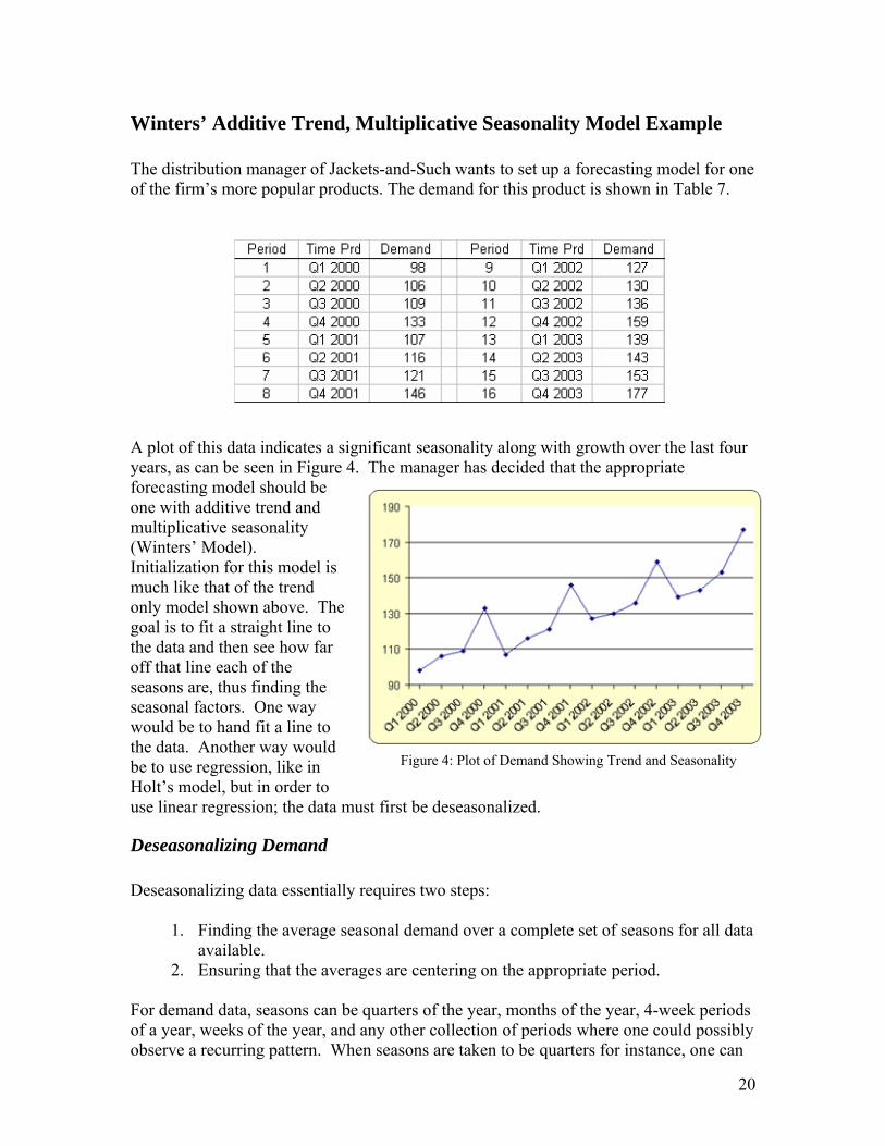
Winters’ Additive Trend, Multiplicative Seasonality Model Example The distribution manager of Jackets-and-Such wants to set up a forecasting model for one of the firm’s more popular products. The demand for this product is shown in Table 7.

plot of this data indicates a significant seasonality along with growth over the last four

nality

the data and then see how far

asons are, thus finding the way

e data. Another way would be to Holt’s model, but in order to use linear m

Deseaso

ires two steps:

. Finding the average seasonal demand over a complete set of seasons for all data

he averages ar

Figure 4: Plot of Demand Showing Trend and Seasonality

Ayears, as can be seen in Figure 4. The manager has decided that the appropriate forecasting model should be one with additive trend and multiplicative seaso(Winters’ Model). Initialization for this model is much like that of the trend only model shown above. The goal is to fit a straight line to

off that line each of the seseasonal factors. One would be to hand fit a line to th

use regression, like in

regression; the data

nalizing Demand

ust first be deseasonalized.

Deseasonalizing data essentially requ

1available.

2. Ensuring that t

For demand data, seasons can be quarters of the year, months of the year, 4-week periods of a year, weeks of the year, and any other collection of periods where one could possibly observe a recurring pattern. When seasons are taken to be quarters for instance, one can

e centering on the appropriate period.

20

find the average deseasonalized quarterly demand by taking averages over any four consecutive quarters. Using the data from Jackets-and-Such, the average quarterly

emand over the first year is d

5.1114

133109106985.2 =

+++=D

Since this is the average over thfirst four periods, this demand average is centered on period 2.5, which is the subscript on the average demand. This can be seen in Table 8where the first set of dark diagonal lines show the 111.5 as the averagover the demand data from 98 to 133. In similar fashion, the average value of 113.5 is found by takinaverage over four consecutive

e

e

g the

uarters starting with period 2.

Table 8: Deseasonalized Calculations

q

8.1134

1071331091065.3 =

+++=D

So that the deseasonalized demand is centered on each period and not between them, each pair of the deseasonalized averages above and below each period must be averaged to get the deseasonalized estimate is as of a certain period, and not between the periods.

6.1122

8.1135.1112

5.25.23 =

+=

+=

DDD

This centered, deseasonalized demand average is shown in the last column of Table 8 where the set of light lines indicate the result of the average of the two numbers, 111and 113.8.

.5 The rest of the centered, deseasonalized averages are also shown in this

olumn.

period of the data being averaged) and there would be no reason to center the average.

c It should be noted that this procedure to deseasonalize the demand is appropriate for seasonal situations where the number of seasons is even. An even number of seasons requires the deseasonalized data be centered. If the number of seasons is odd, as would be the case if the data were broken into say thirteen four-week seasons, then when all of the seasons are averaged, the resulting average would occur on the middle period (in the case of thirteen periods, the seventh

21

Determining the Initial Forecasting Factors

e as d averages can be regressed on the

eriod number with the result fo

sonal factors must be determined to complete the model. This equires three steps.

emand,

period.

tep 1 can be done by finding the straight line estimate of deseasonalized demand

+= (30)

or instance, for period 4 the estimate is

=×+=D

nality from Step 4 for any period is the ratio of the actual demand to e demand forecast

Once the data has been deseasonalized, finding the level and trend factors is the samwith Holt’s trend only model. The deseasonalizep r this data that

L0 = 100.8 T0 = 3.5 Finally, the initial sear

tD̂ 1. Finding an estimate of the straight line fit of deseasonalized d2. Determining an estimate of the seasonality for each 3. Averaging the estimates across all similar seasons.

S

00ˆ tTLD t

F

8.1145.348.100ˆ 4

The estimate of seasoth

t

tt D

DS ˆ~= (31)

gain, using period 4, this estimate is A

16.1 8.114ˆ

44 ≅==

DS

This number indicates that the actual dema

133~ 4D

nd for period 4 is approximately 16% higher than the straight-line deseasonalized fit.

22

Once an estimate has been calculated for each demand observation (as shown in Figure 5 – with arrows indicating all quarter 4 differences), Step 3 is used to find the initial seasonal factors. For any given “season”, all estimates for that season are averaged for an

Figure 5: Seasonal Factor for Q4

overall initial seasonal factor for the given season. Thus, one seasonal factor is obtained for each of the p seasons by averaging over k observations of that season.

k

SSSSS ptptptt

pt

KK

++++= +++

∈32

},,2,1{

~~~~ (32)

For the 4th quarter, this would be

13.14

13.111.113.116.14

~~~161284

4 ≅+++

=+++

=SSSS

S

Doing this for each season, the four seasonal factors are found as

13.1;98.0;96.0;94.0 4111 ≅≅≅≅ SSSS These calculations are summarized in Table 9.

Forecasting with Winters’ Model Now that the initial level, trend, and seasonal factors have been obtained for Winters’ model, the model can be trained and then used to forecast the desired future periods.

23

Table 9: Seasonal Estimates and Initial Seasonal Factors

To train the model, the initial factors are used to forecast for the first period. In this case, the first forecast is for Quarter 1 of 2000. This forecast is obtained using Equation (27) and 0.9894.0)5.38.100()()( 100111 ≅+=+=⇒+= ++ STLFSTLF tttt Once this forecast has been made, the assumption is that time moves forward and the period 1 demand is observed to be 98. With the observation of more demand, the level, trend and seasonal factors can be updated as was the case with the previous trend only model. To do this, Equations (32)-(34) are used. First, the level factor is updated with the assumption that α=0.25 as

3.104)5.38.100(75.094.0

9825.0

))(1(

))(1(

001

11

11

=++=

+−+=

⇒+−+= −−

TLSD

L

TLSD

L ttt

tt

αα

αα

Next, the trend factor is updated with the assumption that β=0.20 as

5.35.38.0)8.1003.104(2.0

)1()()1()(

0011

11

=×+−=−+−=

⇒−+−= −−

TLLTTLLT tttt

ββββ

24

Finally, the seasonal factor for period 1, which happens to be the one used for any first quarter forecasts, is updated. The smoothing parameter is γ=0.15.

94.094.0)15.01(3.104

9815.0

)1(

)1(

11

15

=−+=

−+=

⇒−+=+

SLD

S

SLD

S tt

tpt

γγ

γγ

Note that this update didn’t change any of the factors and this is because the forecast was very accurate for the first period. Once the parameters have been updated, Equation 27 can be used once again to forecast the next period, period 2. The rest of the computations for this forecasting and updating are shown in Table 10.

Table 10: Forecasting and Updating for Jackets-And-Such

Summary The prior sections have provided the reader with an introduction to a number of fundamental approaches and models to time series forecasting and illustrated their computational process. Some forecast models like Winters’ are complicated, involving numerous mathematical equations with the inherent required notation to manage the needed computations. But as complicated as they might be, using these statistical models can help reduce forecast errors to manageable levels without significant levels of every-

25

day human interaction. These models are designed to remove systematic error and can be helpful in doing just that when implemented correctly. While more elaborate models like ARIMA and X11 have been proposed3, the set described above have proved to be the primary forecasting tools used in practice. Practice has also shown that forecasts, no matter how sophisticated a model employed, will still have forecast errors. Perfect forecasts, while a laudable goal, can’t be attained because random behavior and dynamic change is always present. The solution? Human input is a critical component to test for reasonableness and handle unforeseeable events. Therefore, the forecast system design needs to combine human oversight management with statistical forecasting models on computer-based systems like SAP’s R/3 system, so that management time can be spent most productively on the numerous tasks within the supply chain.

Forecasting References

Armstrong, J. S. (2001c), “Extrapolation for time-series and cross-sectional data,” in J. S. Armstrong (ed.), Principles of Forecasting. Norwell, MA: Kluwer Academic Press.

Box, G. E. P., Jenkins, G. M., and Reinsel, G. C. (1994). Time Series Analysis, Forecasting and Control, 3rd ed. Prentice Hall, Englewood Clifs, NJ.

Chatfield, C. (1996). The Analysis of Time Series, 5th ed., Chapman & Hall, New York, NY.

Gardner, E. S. Jr. (1985), “Exponential smoothing: The state of the art,” Journal of Forecasting, 4, 1-28.

C. C Holt (1957) Forecasting seasonals and trends by exponentially weighted moving averages, ONR Research Memorandum, Carnegie Institute 52.

Nelson, C. R. (1973). Applied Time Series Analysis for Managerial Forecasting, Holden-Day, Boca-Raton, FL.

Makradakis, S., Wheelwright, S. C. and McGhee, V. E. (1983). Forecasting: Methods and Applications, 2nd ed., Wiley, New York, NY.

P. R. Winters (1960) Forecasting sales by exponentially weighted moving averages, Management Science 6, 324–342.

3 The interested reader can use the citations listed in the references to explore their features.

26

Time Series Forecasting Problems 1. Using the data above in Table 4 for Bike 3023, forecast demand using the BES

model, but with an α=0.4. Compare this forecast to the example with an α=0.2. 2. Using the data above in Table 4 for Bike 3023, forecast demand using a five-period

moving average and a five period weighted moving average for periods 7 through 13. For the weighted moving average, use the weights 0.5, 0.4, 0.3, 0.2, and 0.1. Compare these two forecasts to the two BES models for Bike 3023, especially with respect to the MAD, MSE, Bias, and TS for periods 7 through 12.

3. Using the data above in Table 4 for Bike 3023, fit an additive trend model to the data

and forecast periods 7 through 15. Compare this forecast model to the two BES models and the two MA models in problems 1 and 2 by commenting on the errors.

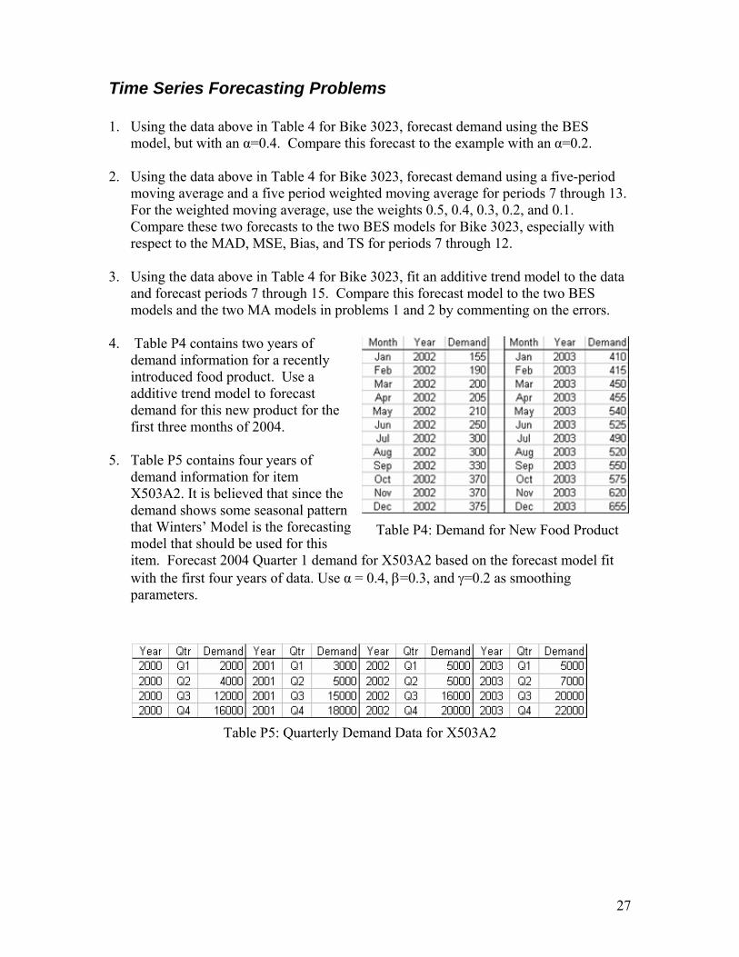
4. Table P4 contains two years of

demand information for a recently introduced food product. Use a additive trend model to forecast demand for this new product for the first three months of 2004.

5. Table P5 contains four years of

demand information for item X503A2. It is believed that since the demand shows some seasonal pattern that Winters’ Model is the fmodel that should be used for thisitem. Forecast 2004 Quarter 1 demand for X503A2 based on the forecast modewith the first four years of data. Use α = 0.4, β=0.3, and γ=0.2 as smoothing parameters.

orecasting

l fit

Table P4: Demand for New Food Product

Table P5: Quarterly Demand Data for X503A2

27

Table P6: Monthly Demand Data for Rain Jacket6. Table P6 contains three years of monthly demand information for a popular classic

rain jacket. Forecast the first six months of demand for this jacket based on forecast model fit with the first four years of data. Use α = 0.4, β=0.3, and γ=0.2 as smoothing parameters.

28

Forecasting with SAP R/3

Introduction and Background The prior section presented a tutorial on basic time series forecasting logic, procedures and performance measures. While we could program these procedures using tools like Visual Basic or Excel spreadsheets, there are several commercial packages available to support business planning. This section illustrates how to employ the SAP R/3 system to conduct forecasting. It shows how to load data, define forecast parameters, obtain forecasts, and review the results from R/3’s forecasting process. The Glow-Bright Corporation case (included in a later section) provides an opportunity to demonstrate the forecasting system within the SAP R/3 system. Below is an example plot of sales in R/3 for part number 40-100C of Glow-Bright. Note that the data exhibits seasonality and an upward trend in historical sales. The R/3 forecasting system employs a time series analysis approach to forecasting, and as such, attempts to find a pattern over time in the historical database, and then extends this pattern into the future. As discussed above, there are a number of models that users may chose to attempt to match historical patterns. Therefore, the system must first have historical data to do the time series analysis for the forecasts.

Loading Historical Data The first step to using the forecast feature of R/3 requires populating the ‘Material Master’ with historical sales data. Since the system used in a learning environment is not an active system with “real” sales data, this historical data must be entered before any forecasting can be done. To enter this data, navigate through the Dynamic Menu within

29

R/3 down to the plant level by making the appropriate entries, as shown below. This will eventually lead to the ‘Forecasting’ tab within the ‘Material Master’ which allows one to use the Forecast Module.

Next, open the ‘Forecasting’ tab of the record for part 40-100C and click on the Consumption Vals button. This opens the table of historical data, as shown below. Note that the first time this table is opened the record will be empty.

30

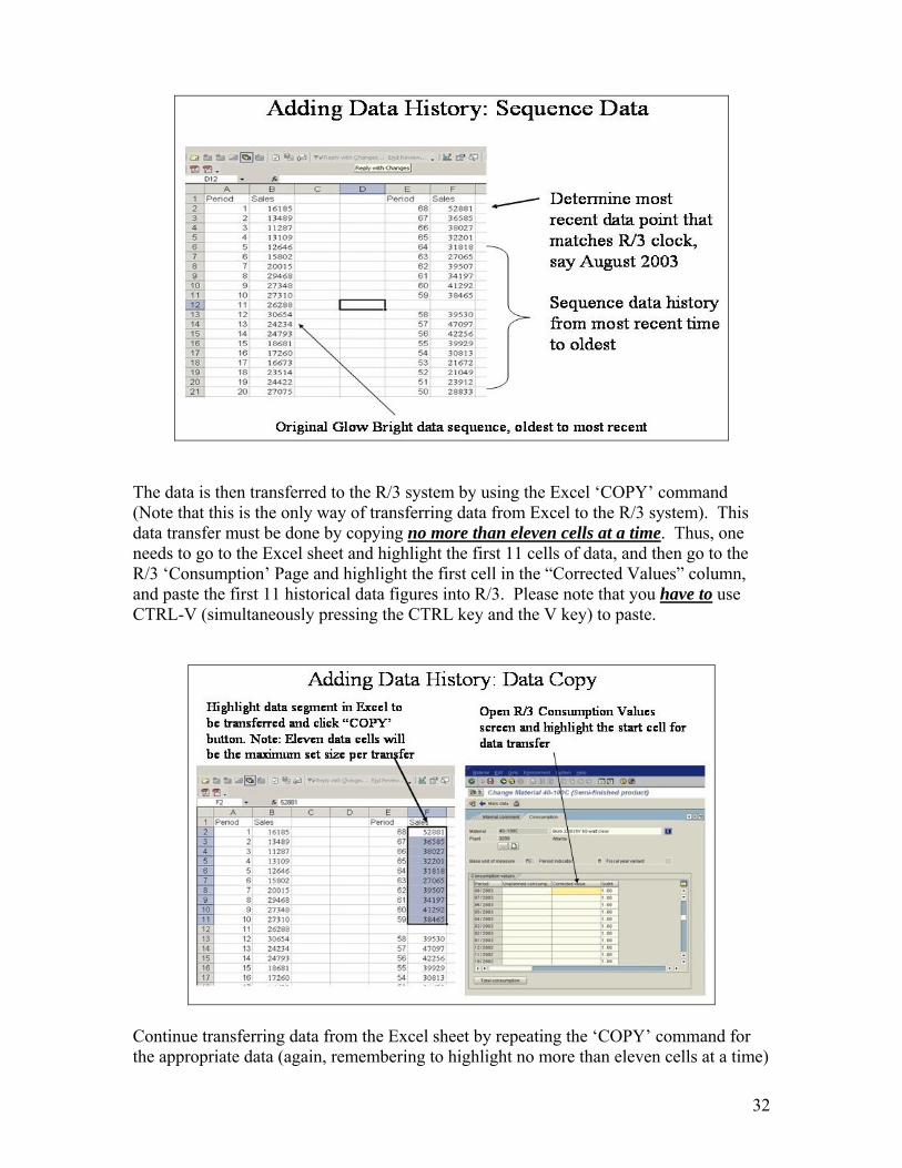
One of the most important issues in using the R/3 forecasting module is the time orientation of the data. This arises because the R/3 system is an operational system with a running clock. Any time you use the system, the system clock will be the current time and date. Thus, the first thing that has to be determined is the current R/3 system time clock date. This will be the time origin reference for forecasting. Another important issue is that the historical data needs to be sequenced from most recent to oldest. The Glow Bright historical sales data is organized in an oldest-to-most recent format – as shown below – and this is the opposite of what is needed.

Assume that the current R/3 system time is August of 2003. This will be assumed to be the time origin point for the sales history. That is, the last month of the sales data should be August of 2003. Next, the data needs to be re-sequenced from most recent to oldest. This can be done very easily in Excel, starting with the data from August 2003 (Period 68 with a demand of 52,881).

31

The data is then transferred to the R/3 system by using the Excel ‘COPY’ command (Note that this is the only way of transferring data from Excel to the R/3 system). This data transfer must be done by copying no more than eleven cells at a time. Thus, one needs to go to the Excel sheet and highlight the first 11 cells of data, and then go to the R/3 ‘Consumption’ Page and highlight the first cell in the “Corrected Values” column, and paste the first 11 historical data figures into R/3. Please note that you have to use CTRL-V (simultaneously pressing the CTRL key and the V key) to paste.

Continue transferring data from the Excel sheet by repeating the ‘COPY’ command for the appropriate data (again, remembering to highlight no more than eleven cells at a time)

32

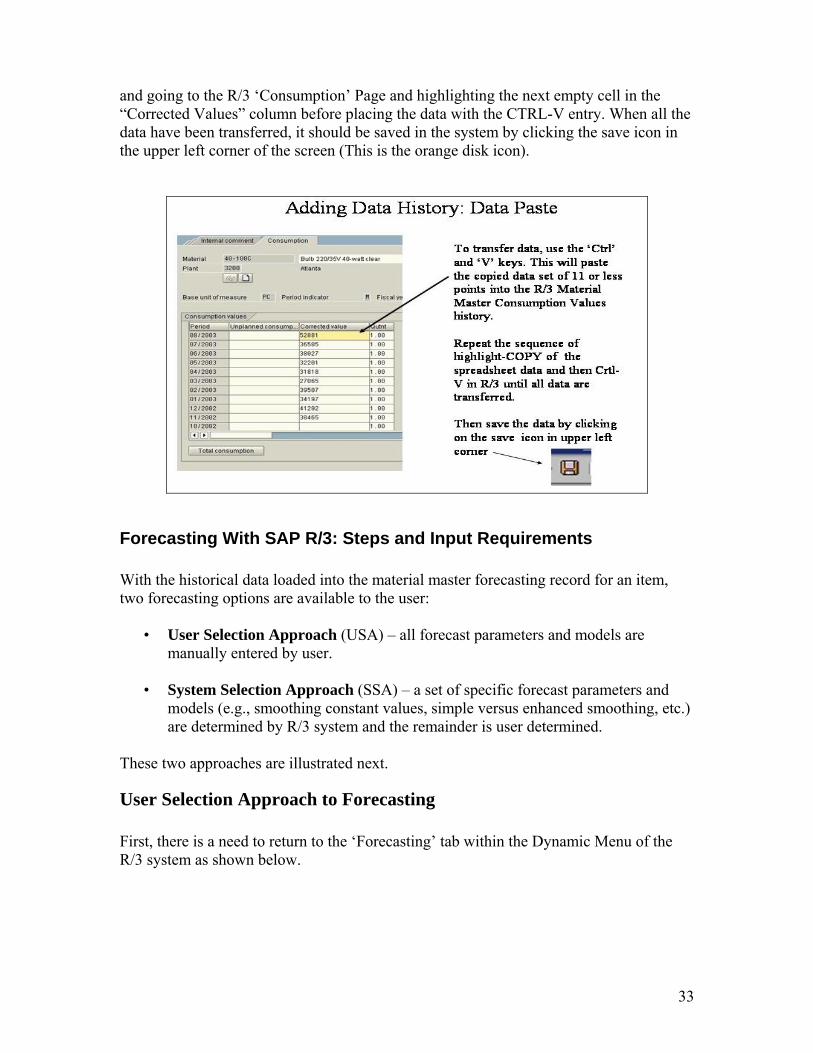
and going to the R/3 ‘Consumption’ Page and highlighting the next empty cell in the “Corrected Values” column before placing the data with the CTRL-V entry. When all the data have been transferred, it should be saved in the system by clicking the save icon in the upper left corner of the screen (This is the orange disk icon).

Forecasting With SAP R/3: Steps and Input Requirements With the historical data loaded into the material master forecasting record for an item, two forecasting options are available to the user:

• User Selection Approach (USA) – all forecast parameters and models are manually entered by user.

• System Selection Approach (SSA) – a set of specific forecast parameters and

models (e.g., smoothing constant values, simple versus enhanced smoothing, etc.) are determined by R/3 system and the remainder is user determined.

These two approaches are illustrated next.

User Selection Approach to Forecasting First, there is a need to return to the ‘Forecasting’ tab within the Dynamic Menu of the R/3 system as shown below.

33

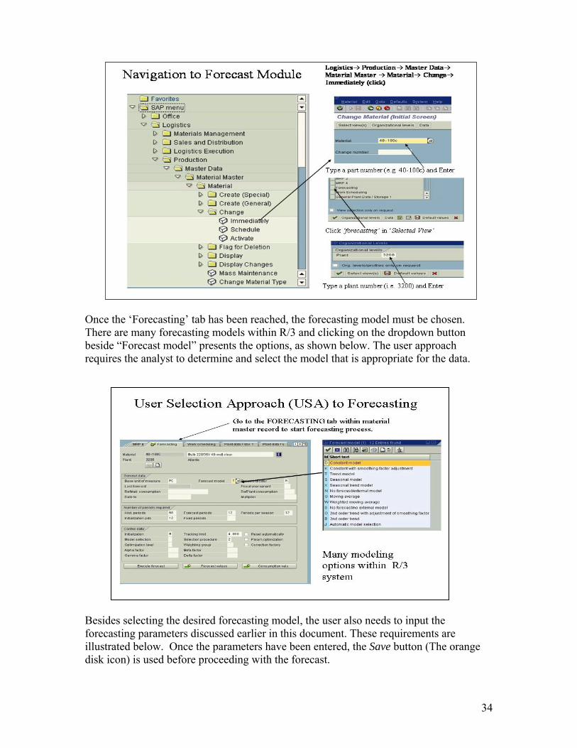
Once the ‘Forecasting’ tab has been reached, the forecasting model must be chosen. There are many forecasting models within R/3 and clicking on the dropdown button beside “Forecast model” presents the options, as shown below. The user approach requires the analyst to determine and select the model that is appropriate for the data.

Besides selecting the desired forecasting model, the user also needs to input the forecasting parameters discussed earlier in this document. These requirements are illustrated below. Once the parameters have been entered, the Save button (The orange disk icon) is used before proceeding with the forecast.

34

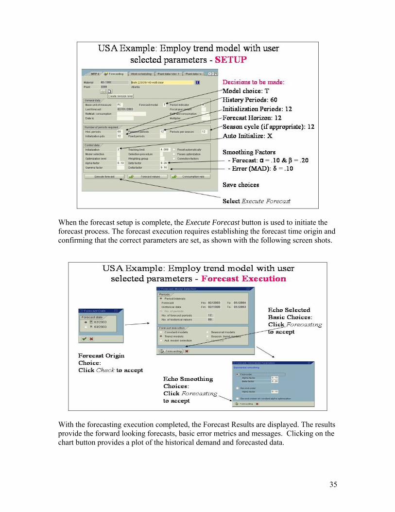
When the forecast setup is complete, the Execute Forecast button is used to initiate the forecast process. The forecast execution requires establishing the forecast time origin and confirming that the correct parameters are set, as shown with the following screen shots.

With the forecasting execution completed, the Forecast Results are displayed. The results provide the forward looking forecasts, basic error metrics and messages. Clicking on the chart button provides a plot of the historical demand and forecasted data.

35

System Selection Approach to Forecasting First, as with the last approach, there is a need to return to the ‘Forecasting’ tab in the Dynamic Menu. This is done through the ‘Material Master’ as highlighted below.

Within the R/3 system, there are a set of features that allow the system to determine the appropriate forecast model (e.g., inclusion of seasonal factors) and the associated

36

smoothing values. As shown below, the user determines which potential model options are available and what level of refinement is desired.

To invoke SSA, the user selects the option the system will use to determine the forecast model and parameter values. The figure below identifies the appropriate entries in the ‘Forecasting’ tab page. For model selection, the options are:

Procedure 1 -The system uses a significance test to determine whether a trend or a seasonal pattern is present, and then selects the forecast model on the basis of the results.

Procedure 2 - The system carries out the forecast using all the models, optimizes

the parameters, and then selects the model with the smallest mean absolute deviation.

For Parameter Optimization, the set indicator (check mark) causes the system to determine the best smoothing factors needed by the given forecast model to minimize errors. The system calculates a number of different parameter combinations and selects the one that produces the lowest mean absolute deviation.

37

While the R/3 system will determine a set of forecast parameter components, the user still must provide a number of inputs, as shown below, to complete the forecast preparation process. With the required user input supplied, click the Execute Forecast button to proceed. The time origin and echo check will take place as illustrated in the previous procedure. If satisfied with the input, click the Forecast button for forecast execution.

38

The Forecast Results report follows the structure as described earlier, with the same features. Check the ‘Forecast message’ tab to determine what has occurred during forecast execution. To see the optimal parameter values, click the check button.

For the Glow-Bright data example, the model included trend and determined the best alpha and beta values, shown below. If satisfied with results, click the save button to save the forecast values and all forecast parameter settings for future use.

39

Summary

This section has demonstrated the steps required to conduct time series forecasting using the SAP R/3 system. It illustrated how to load data into the material master record, highlighted the required forecast parameter options that are available to the user and showed the forecast execution steps.

For more information about the SAP R/3 forecast module, the interested reader can use the online help system. It provides more extensive documentation of system features and requirements.

40

Creating Part Numbers

While the SAP R/3 system has about 20 blank part numbers that can be used for forecasting, it can be advantageous to create unique part numbers for use. The exhibits below illustrate the required steps: Navigate to Create Screen to initiate creation process.

Enter initial required data of unique part number. Using drop down menus for industry sector and material type, select appropriate options and click check mark.

41

Assign part number to Forecasting and Plant master data set.

Complete minimal data requirements for master.

42

With entries complete, save new part master for future use.

43

Glow-Bright Corporation Case4

John Hartness, plant manager for Glow-Bright Corporation's Atlanta plant, sat at his desk reviewing recent production reports for the last accounting period. According to the reports, the plant had been operating near the highest output level in its history for their model 40-100C, a 40 watt clear incandescent light bulb. Glow-Bright's other product lines were also experiencing strong sales. As John sat there feeling proud of the increased output that the plant had attained, the phone rang and broke into his thoughts. It was Dan Martin, vice president of manufacturing, calling for his weekly check-in with John to discuss operations at the plant. Looking over his production reports, John turned to the warehouse reports to refresh some points in his mind. "Dan, the warehouse reports have shown excessive costs. The Atlanta warehouse has had to purchase another forklift and hire an operator for it. Thompson, at the Chicago facility, has indicated that they have had to rent temporary space at the public warehouse around the corner. We may have to expand or lease more space." A few seconds of silence occurred at the other end of the phone. Then Martin responded, "Before we consider investing for expansion or committing ourselves to a lease, we must be certain that the increased demand is genuine. In the next week, discuss with marketing what demand we can anticipate for the 40-100C bulb in the future. Keep in mind when you talk to them that those marketing forecasts are never right. It sounds like we need to act on this issue quickly, so let me know your opinion as soon as possible." After hanging up the phone, Hartness looked at his watch. It was almost noon. He got up, pulled his coat off the hook, and headed out of his office door for a luncheon meeting with the local Kiwanis Club planning committee. As he went through the outer office, he stopped to talk to his secretary, Emma Castaro. "Emma, will you please go through our past sales records and list the units sold in each period for the last six years for the 40-100C bulb. Also, bring me the forecast reports supplied by marketing for those same months. Please have them on my desk this afternoon, so that I can review what has been happening." Later that afternoon, Emma came into Hartness' office with the sales and forecast data. As John looked over the sheets, shown in Tables 1 and 2, Emma said, "I called marketing and asked for the forecasts, which production planning uses. They sent over this report." She handed John the forecasts (Table 2) for the same period, as compiled by the marketing department. Attached to the forecast report was a copy of the standard form letter (Exhibit 1) from Harold Wilson, vice-president of marketing, to the district sales managers. He was requesting the annual sales force forecasts for the coming year. Emma indicated it was sent to give Hartness background on how the annual forecast was developed. 4 Case developed by Vincent A. Mabert, Indiana University. Revised 8/23/2003

44

Basically, the sales force is polled as to their expectations for the coming year. These forecasts are made at the end of each year. The district and home office managers then make adjustments to remove any bias that the salesmen have. The forecasts are then given to the production department to use in laying out the manufacturing schedule. John looked at the actual and forecast sales volume, Tables 1 and 2. He pulled his new Cross pencil from his shirt pocket and started checking the errors between what was forecasted and the actual sales. Then the telephone rang. It was Roger Steel, director of production planning. He called to find out where John was. Hartness was already half an hour late for the weekly plant meeting of department heads. John hung up the phone and headed for the conference room. As he went down the hall, he knew it would be a long night. He needed to get the new laptop PC from the Industrial Engineering Department to assist in analyzing the forecast and actual sales volume. Company Background Glow-Bright manufactures multiple lighting product lines at the Atlanta plant: both incandescent (25, 40, 60, 75 watts, etc.) and florescent light (10, bulbs - 10, 20, and 40 watts) in various wattage levels and frosting finishes for residential applications. The Atlanta twelve-acre site has two plants, employing about 850 employees. Plant 3200 produces incandescent bulbs, while Plant 3400 assembles florescent lights. Glow-Bright distributes its light bulbs through regional warehouses to wholesalers, major box retailers like Lowes and Home Depot, and discount chains. The wholesalers then sell directly to retail outlets like hardware stores. The National Lighting Institute (NLI) has estimated that sales of lights are broken into three categories: residential lighting, commercial lighting and specialty applications. The sales seem to be linked to the general economic conditions of the country. NLI routinely reports the sales level for the lighting industry. Table 3 lists the industry experience for the last six years. Study Guide Questions

1. Evaluate the current forecasting procedures at Glow-Bright. Are they adequate for manufacturing needs?

2. How would you design and implement a forecasting system at Glow-Bright?

45

GLOW-BRIGHT CORPORATION Atlanta, GA (Exhibit 1)

October 20, 2002 To: District Managers C.B. Ernst - Tulsa R.E. Edmunster Beach Associates Haffer & Allison - Portland Haffer & Allison - Seattle Bill Tellson Alloy Products Company Subject: Unit Sales Product Forecast for Next Year This is the time of year that we are making plans for next year's production. So that we can meet your customer requirements and, at the same time, operate our facilities at the most efficient level, we need your very best efforts in estimating sales by product line. Please complete the attached forms and return to us by December 10. You should take as positive an attitude as possible to get the most meaningful information. While it is true that in many cases customers will tell you that they do not know what their requirements will be, there may be other individuals within the company who can give you better information. Keep in mind that the firm itself must make its own plans in advance and conduct its own surveys. Among the things that you might want to consider in addition to asking key individuals within the company are:

a. The general forecast of economic conditions in your territory b. The projected housing starts and commercial construction for the area. c. Whether or not you feel Glow-Bright will be getting increases, decreases, or the

same share of the business from specific customers. d. Whether or not you will "break in" with new customers. e. Whether or not you will lose customers because of problems.

For the last couple of years, we have been caught short, with resulting loss of business because of poor deliveries. In all cases, we would have been current on deliveries had the forecast been accurate. It is to our benefit to consider this a major assignment. Harold Wilson: mrm

46

Table 1: 40-100C Unit Sales (Cartons)

Month 1998 1999 2000 2001 2002 20031 16,185 24,234 31,768 30,117 28,228 34,197 2 13,489 24,793 24,894 26,885 28,833 39,507 3 11,287 18,681 18,070 19,686 23,912 27,065 4 13,109 17,260 21,138 15,607 21,049 31,818 5 12,646 16,673 19,750 16,795 21,672 32,201 6 15,802 23,514 32,474 25,172 30,813 38,027 7 20,015 24,422 32,053 27,731 39,929 36,585 8 29,468 27,075 35,923 27,951 42,256 52,881 9 27,348 26,793 35,248 23,729 47,097 41,933

10 27,310 30,279 23,315 28,034 39,530 41,701 11 26,288 26,118 28,252 26,363 38,465 46,017 12 30,654 30,986 28,879 27,675 41,292 45,027

Table 2: 40-100C Forecast Units (Cartons) Month 1998 1999 2000 2001 2002 2003

1 27,000 31,000 32,000 34,000 35,000 35,000 2 27,000 31,200 32,000 34,000 35,000 35,000 3 29,000 31,800 33,000 34,000 35,000 36,000 4 29,000 31,400 34,000 34,000 35,000 38,500 5 29,000 31,200 34,000 35,500 36,000 38,500 6 30,000 31,000 33,000 35,400 36,000 38,500 7 31,000 30,800 32,500 36,000 35,000 38,000 8 32,000 30,600 32,500 33,000 35,000 37,000 9 29,000 30,400 32,500 33,000 35,000 36,000

10 29,000 30,000 32,500 32,400 35,000 37,000 11 28,600 30,000 32,000 32,000 34,000 36,000 12 28,000 30,000 32,000 32,000 34,000 36,000

Table 3: Lighting Sales Estimates for NLI ($ 000)

Month 1998 1999 2000 2001 2002 20031 67,477 90,462 110,862 102,738 136,985 172,154 2 65,815 91,846 118,708 83,354 124,892 168,369 3 69,623 97,177 111,008 90,208 121,169 176,662 4 96,200 132,123 148,692 126,062 176,985 223,954 5 117,508 165,669 174,092 149,862 216,254 241,777 6 135,662 161,877 176,985 148,985 222,769 252,185 7 138,885 153,331 172,031 152,754 222,323 256,238 8 135,138 152,954 158,815 160,985 222,231 245,769 9 136,469 154,192 149,062 160,062 227,062 244,954

10 138,554 153,323 152,431 155,846 226,708 249,969 11 138,000 153,831 155,700 161,215 210,900 236,146 12 144,292 157,877 147,662 163,985 210,169 242,400

47