1

Chapter 15

Demand Management & Forecasting

Demand Management

Qualitative Forecasting Methods

Simple & Weighted Moving Average Forecasts

Exponential Smoothing

Simple Linear Regression

2

Demand Management

A

Independent Demand:Finished Goods

B(4) C(2)

D(2) E(1) D(3) F(2)

Dependent Demand:Raw Materials, Component parts,Sub-assemblies, etc.

3

Independent Demand: What a firm can do to manage it.

Can take an active role to influence demand

Can take a passive role and simply respond to demand

4

What Is Forecasting?

Process of predicting a future event

Underlying basis of all business decisions– Production– Inventory– Personnel– Facilities

Sales will be $200 Million!

5

Types of Forecasts by Time Horizon

Short-range forecast– – Job scheduling, worker assignments

Medium-range forecast– – Sales & production planning, budgeting

Long-range forecast– – New product planning, facility location

6

Types of Forecastsby Item Forecast

Economic forecasts– Address business cycle– e.g., inflation rate, money supply etc.

Technological forecasts– Predict technological change– Predict new product sales

Demand forecasts– Predict existing product sales

7

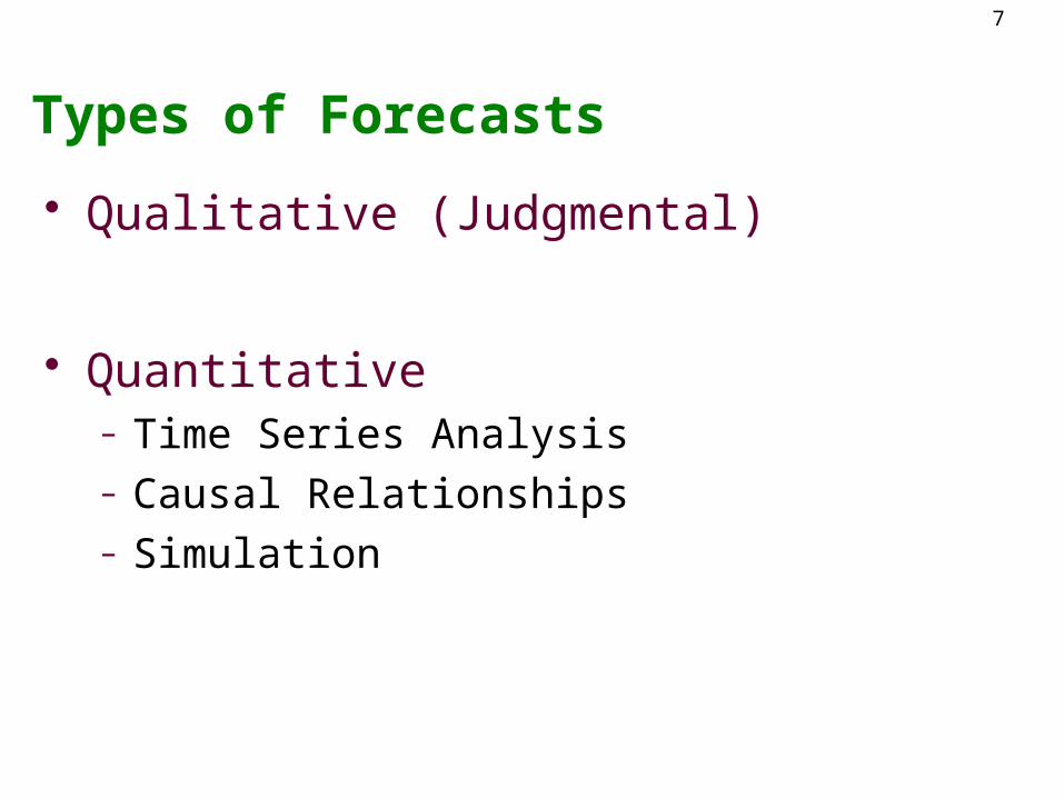
Types of Forecasts

Qualitative (Judgmental)

Quantitative– Time Series Analysis– Causal Relationships– Simulation

8

Components of Demand

Average demand for a period of time Trend Seasonal element Cyclical elements Random variation Autocorrelation

9

Finding Components of Demand

1 2 3 4

x

x xx

xx

x xx

xx x x x

xxxxxx x x

xx

x x xx

xx

xx

x

xx

xx

xx

xx

xx

xx

x

x

Year

Sal

es

Seasonal variation

Linear

Trend

10

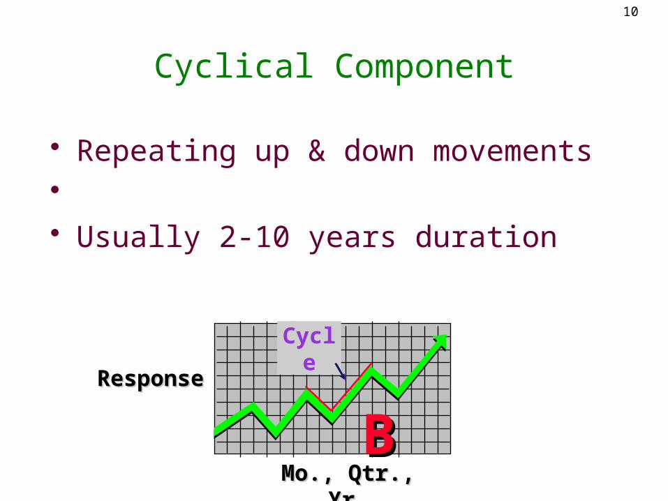
Cyclical Component

Repeating up & down movements Usually 2-10 years duration

Mo., Qtr., Yr.Mo., Qtr., Yr.

ResponseResponseCycle

BB

11

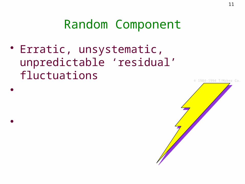
Random Component

Erratic, unsystematic, unpredictable ‘residual’ fluctuations

© 1984-1994 T/Maker Co.

12

Qualitative Methods

Grass Roots

Market Research

Panel Consensus

Executive Judgment

Historical analogy

Delphi Method

Qualitative

Methods

13

Delphi Methodl. Choose the experts to participate. There should be

a variety of knowledgeable people in different areas.

2. Through a questionnaire (or E-mail), obtain forecasts (and any premises or qualifications for the forecasts) from all participants.

3. Summarize the results and redistribute them to the participants along with appropriate new questions.

4. Summarize again, refining forecasts and conditions, and again develop new questions.

5. Repeat Step 4 if necessary. Distribute the final results to all participants.

14

CausalModels

Quantitative Forecasting Methods

QuantitativeForecasting

Time SeriesModels

LinearRegression

ExponentialSmoothing

TrendProjection

MovingAverage

15

Time Series Analysis

Time series forecasting models try to predict the future based on past data.

You can pick models based on:

1. Time horizon to forecast

2. Data availability

3. Accuracy required

4. Size of forecasting budget

5. Availability of qualified personnel

16

Simple Moving Average Formula

F = A + A + A +...+A

ntt-1 t-2 t-3 t-n

The simple moving average model assumes an average is a good estimator of future behavior.

The formula for the simple moving average is:

Ft = Forecast for the coming period N = Number of periods to be averagedA t-1 = Actual occurrence in the past period for up to “n” periods

17

Forecasting Example # 1

Weekly Video RentalsWeek Video Rentals

1 6542 6583 6654 6725 6736 6717 6938 6949 70110 70311 70212 710

Weekly Video Rentals

620630640650660670680690700710720

1 2 3 4 5 6 7 8 9 10 11

Week

Vide

os R

ente

d

18

Forecasting Video Rentals With Moving Averages

WeekVideo

Rentals1 6542 6583 6654 6725 6736 6717 6938 6949 70110 70311 70212 710

F = A + A + A +...+A

ntt-1 t-2 t-3 t-n

Question: What are the 2-week and 4-week moving average forecasts for video rentals?

Which forecast would you prefer?

Week Demand 2-Week 4-Week1 6542 6583 665 6564 672 661.55 673 668.5 662.256 671 672.5 667.007 693 672 670.258 694 682 677.259 701 693.5 682.75

10 703 697.5 689.7511 702 702 697.7512 710 702.5 700.00

Calculating the moving averages gives us:

©The McGraw-Hill Companies, Inc., 2000

19

20

2 Period Moving Average( Weekly Video Rentals)

650

660

670

680

690

700

710

720

3 4 5 6 7 8 9 10 11 12 13

Week

Vid

eo

Ren

tals

Forecast

Actual

Which Forecast Would You Prefer?

4 Period Moving Average(Weekly Video Rentals)

650

660

670

680

690

700

710

720

5 6 7 8 9 10 11 12 13

Week

Vid

eo

Ren

tals

Forecast

Actual

21

Forecasting Example # 2Quarterly Sales Data (Acme Tool Company)

Quarter Sales

1 550

2 400

3 350

4 600

5 750

6 500

7 400

8 650

9 850

10 600

11 450

12 700

Quarterly Sales Data(Acme Tool Company)

0

100

200

300

400

500

600

700

800

900

3 4 5 6 7 8 9 10 11 12

Quarter

Qu

arte

rly

Sal

es

22

Forecasting Quarterly Sales With Moving Averages

Quarter Demand1 5502 4003 3504 6005 7506 5007 4008 6509 85010 60011 45012 700

F = A + A + A +...+A

ntt-1 t-2 t-3 t-n

Question: What are the 2-week and 4-week moving average forecasts for Quarterly Sales

Which forecast would you prefer?

23

Quarter Demand 2-Week 4-Week1 5502 4003 350 4754 600 3755 750 475 4756 500 675 5257 400 625 5508 650 450 562.59 850 525 575

10 600 750 60011 450 725 62512 700 525 637.5

Calculating the moving averages gives us:

24

2 Period Moving Average(Acme Tool Company)

0

100

200

300

400

500

600

700

800

900

3 4 5 6 7 8 9 10 11 12 13

Quarter

Qu

art

erl

y S

ale

s

Forecast

Actual

Which Forecast Would You Prefer?

4 Period Moving Average(Acme Tool Company)

0

100

200

300

400

500

600

700

800

900

5 6 7 8 9 10 11 12 13

Quarter

Qu

arte

rly

Sal

es

Forecast

Actual

25

Weighted Moving Average Formula

F = w A + w A + w A +...+w At 1 t-1 2 t-2 3 t-3 n t-n

w = 1ii=1

n

While the moving average formula implies an equal weight being placed on each value that is being averaged, the weighted moving average permits an unequal weighting on prior time periods.

wt = weight given to time period “t” occurrence. (Weights must add to one.)

The formula for the weighted average is:

26

Weighted Moving Average Problem (1) Data

Weights: t-1 .5t-2 .3t-3 .2

Week Demand1 6502 6783 7204

Question: Given the weekly demand and weights, what is the forecast for the 4th period or Week 4?

27

Weighted Moving Average Problem (1) Solution

Week Demand Forecast1 6502 6783 7204 693.4

28

Weighted Moving Average Problem (2) Data

Weights: t-1 .7t-2 .2t-3 .1

Week Demand1 8202 7753 6804 655

Question: Given the weekly demand information and weights, what is the weighted moving average forecast of the 5th period or week?

29

Weighted Moving Average Problem (2) Solution

Week Demand Forecast1 8202 7753 6804 6555 672

30

Exponential Smoothing Model

Ft = Ft-1 + (At-1 - Ft-1)

Ft = At-1 +(1- )Ft-1

Or, Equivalently

= smoothing constantWhere,

Ft = Forecast for period tAt = Actual value in period t

Note:

31

Ft = At - 1 + (1-)At - 2 + (1- )2·At - 3

+ (1- )3At - 4 + ... + (1- )t-1·A0

– Ft = Forecast value

– At = Actual value

= Smoothing constant

Exponential Smoothing Expansion

32

Forecasting Weekly Video Rentals With Exponential Smoothing

Question: Given the weekly video rental data, what are the exponential smoothing forecasts for periods 2-13 using =0.10 and =0.60?

Assume F1=A1

WeekVideo

Rentals1 6542 6583 6654 6725 6736 6717 6938 6949 70110 70311 70212 710

33

WeekVideo

Rentals =.1 =.61 654 654.00 654.002 658 654.00 654.003 665 654.40 656.404 672 655.46 661.565 673 657.11 667.826 671 658.70 670.937 693 659.93 670.978 694 663.24 684.199 701 666.32 690.08

10 703 669.78 696.6311 702 673.11 700.4512 710 675.99 701.3813 679.40 706.55

Forecasts

Calculating the Exponential smoothing forecasts gives us:

34

Which Forecast Would You Prefer?Exponential Smoothing (Weekly Video Rentals)

=.1

620

630

640

650

660

670

680

690

700

710

720

2 3 4 5 6 7 8 9 10 11 12 13

Week

Vid

eo R

enta

ls

Forecast

Actual

Exponential Smoothing (Weekly Video Rentals)=.6

620

630

640

650

660

670

680

690

700

710

720

2 3 4 5 6 7 8 9 10 11 12 13

Week

Vid

eo R

enta

ls

Forecast

Actual

35

Forecasting Quarterly Sales for the Acme Tool Company With Exponential Smoothing

Question: Given the quarterly sales data, what are the exponential smoothing forecasts for periods 2-13 using =0.10 and =0.60?

Assume F1=A1

Quarter Sales1 5502 4003 3504 6005 7506 5007 4008 6509 85010 60011 45012 700

36

WeekQuarterly

Sales =.1 =.61 550.00 550.00 550.002 400.00 550.00 550.003 350.00 535.00 460.004 600.00 516.50 394.005 750.00 524.85 517.606 500.00 547.37 657.047 400.00 542.63 562.828 650.00 528.37 465.139 850.00 540.53 576.05

10 600.00 571.48 740.4211 450.00 574.33 656.1712 700.00 561.90 532.4713 575.71 632.99

Forecasts

Calculating the Exponential smoothing forecasts gives us:

37

Exponential Smoothing (Acme Tool Company)=.1

200

300

400

500

600

700

800

900

2 3 4 5 6 7 8 9 10 11 12 13

Quarter

Qu

arte

rly

Sal

esActual

Forecasted

Which Forecast Would You Prefer?

Exponential Smoothing (Acme Tool Company)=.6

200

300

400

500

600

700

800

900

2 3 4 5 6 7 8 9 10 11 12 13

Quarter

Qu

arte

rly

Sal

es

Actual

Forecasted

38

Ft = At - 1 + (1- )At - 2 + (1- )2At - 3 + ...

Forecast Effects of Smoothing Constant

Weights

Prior Period

2 periods ago

(1 - )

3 periods ago

(1 - )2

=

= 0.10

= 0.90

39

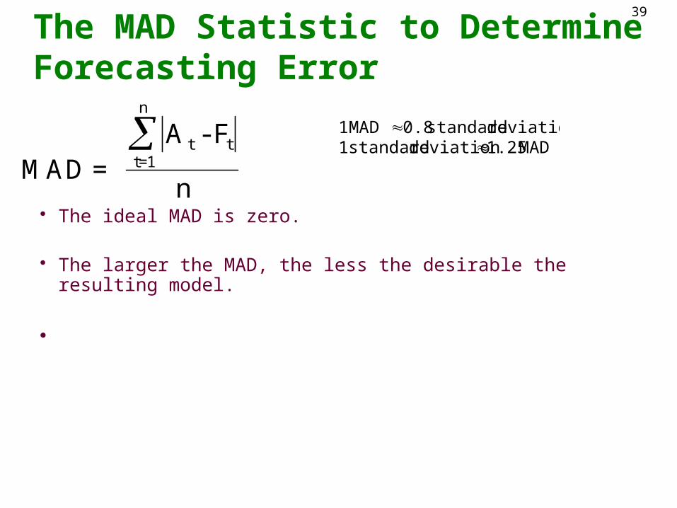
The MAD Statistic to Determine Forecasting Error

MAD = A - F

n

t tt=1

n

MAD 1.25 deviation standard 1deviation standard 0.8 MAD 1

The ideal MAD is zero.

The larger the MAD, the less the desirable the resulting model.

40

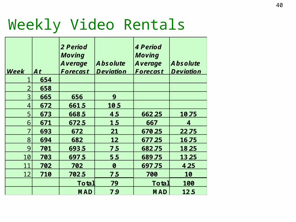
Weekly Video Rentals

Week At

2 Period Moving Average Forecast

Absolute Deviation

4 Period Moving Average Forecast

Absolute Deviation

1 6542 6583 665 656 94 672 661.5 10.55 673 668.5 4.5 662.25 10.756 671 672.5 1.5 667 47 693 672 21 670.25 22.758 694 682 12 677.25 16.759 701 693.5 7.5 682.75 18.25

10 703 697.5 5.5 689.75 13.2511 702 702 0 697.75 4.2512 710 702.5 7.5 700 10

Total 79 Total 100MAD 7.9 MAD 12.5

41

Quarterly Sales (Acme Tool Company)

Quarter At

2 Period Moving Average Forecast

Absolute Deviation

4 Period Moving Average Forecast

Absolute Deviation

1 5502 4003 350 475 1254 600 375 2255 750 475 275 475 2756 500 675 175 525 257 400 625 225 550 1508 650 450 200 562.5 87.59 850 525 325 575 275

10 600 750 150 600 011 450 725 275 625 17512 700 525 175 637.5 62.5

Total 2150 Total 1050MAD 215 MAD 131.25

42

WeekVideo

Rentals =.1Absolute Deviation =.6

Absolute Deviation

1 654 654.00 654.002 658 654.00 4.00 654.00 4.003 665 654.40 10.60 656.40 8.604 672 655.46 16.54 661.56 10.445 673 657.11 15.89 667.82 5.186 671 658.70 12.30 670.93 0.077 693 659.93 33.07 670.97 22.038 694 663.24 30.76 684.19 9.819 701 666.32 34.68 690.08 10.92

10 703 669.78 33.22 696.63 6.3711 702 673.11 28.89 700.45 1.5512 710 675.99 34.01 701.38 8.62

MAD 23.09 MAD 7.96

A Comparison of Exponential Smoothing Forecasts (Video Rentals)

43

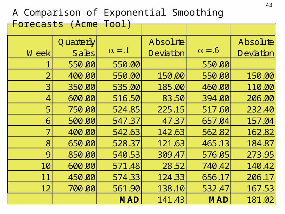
WeekQuarterly

Sales =.1Absolute Deviation =.6

Absolute Deviation

1 550.00 550.00 550.002 400.00 550.00 150.00 550.00 150.003 350.00 535.00 185.00 460.00 110.004 600.00 516.50 83.50 394.00 206.005 750.00 524.85 225.15 517.60 232.406 500.00 547.37 47.37 657.04 157.047 400.00 542.63 142.63 562.82 162.828 650.00 528.37 121.63 465.13 184.879 850.00 540.53 309.47 576.05 273.95

10 600.00 571.48 28.52 740.42 140.4211 450.00 574.33 124.33 656.17 206.1712 700.00 561.90 138.10 532.47 167.53

MAD 141.43 MAD 181.02

A Comparison of Exponential Smoothing Forecasts (Acme Tool)

44

Tracking Signal Formula The TS is a measure that indicates whether the

forecast average is keeping pace with any genuine upward or downward changes in demand.

Depending on the number of MAD’s selected, the TS can be used like a quality control chart indicating when the model is generating too much error in its forecasts.

The TS formula is:

TS =RSFE

MAD=

Running sum of forecast errors

Mean absolute deviation

45

= 0.1

Actual (At)

Forecast (Ft)

Forecast Error

Running Sum of Forecast Errors

Absolute Deviation

Sum of Abs. Dev. MAD

Tracking Signal

1 550.00 550.002 400.00 550.00 -150.00 -150.00 150.00 150.00 150.00 -1.003 350.00 535.00 -185.00 -335.00 185.00 335.00 167.50 -2.004 600.00 516.50 83.50 -251.50 83.50 418.50 139.50 -1.805 750.00 524.85 225.15 -26.35 225.15 643.65 160.91 -0.166 500.00 547.37 -47.37 -73.72 47.37 691.02 138.20 -0.537 400.00 542.63 -142.63 -216.34 142.63 833.64 138.94 -1.568 650.00 528.37 121.63 -94.71 121.63 955.28 136.47 -0.699 850.00 540.53 309.47 214.76 309.47 1264.75 158.09 1.36

10 600.00 571.48 28.52 243.29 28.52 1293.27 143.70 1.6911 450.00 574.33 -124.33 118.96 124.33 1417.60 141.76 0.8412 700.00 561.90 138.10 257.06 138.10 1555.71 141.43 1.82

Quarterly Sales Data - Acme Tool Company

Calculating Tracking Signals for the Exponential Smoothing Forecasts From the Acme Tool Company Example

46

Tracking Signal (Weekly Video Rentals)=0.1

0

2

4

6

8

10

12

2 3 4 5 6 7 8 9 10 11 12

Forecast Period

Tra

ckin

g S

ign

al

Tracking Signal

Tracking Signal (Acme Tool Company)=0.1

-2.5

-2

-1.5

-1

-0.5

0

0.5

1

1.5

2

2.5

2 3 4 5 6 7 8 9 10 11 12

Forecast Period

Tra

ckin

g S

ign

al

Tracking Signal

Tracking Signal Charts

47

Linear Trend Projection

Used for forecasting linear trend line Assumes relationship between response

variable Y & time X is a linear function

Estimated by least squares method– Minimizes sum of squared errors

49

Correlation

Answers ‘how strong is the linear relationship between 2 variables?’

Coefficient of correlation used– Sample correlation coefficient denoted r– Values range from -1 to +1– Measures degree of association

Used mainly for understanding

51

Web-Based Forecasting: CPFR Defined

Collaborative Planning, Forecasting, and Replenishment (CPFR) a Web-based tool used to coordinate demand forecasting, production and purchase planning, and inventory replenishment between supply chain trading partners.

Used to integrate the multi-tier or n-Tier supply chain, including manufacturers, distributors and retailers.

CPFR’s objective is to exchange selected internal information to provide for a reliable, longer term future views of demand in the supply chain.

CPFR uses a cyclic and iterative approach to derive consensus forecasts.

52

Web-Based Forecasting: Steps in CPFR

1. Creation of a front-end partnership

agreement

2. Joint business planning

3. Development of demand forecasts

4. Sharing forecasts

5. Inventory replenishment