Delineating GroundwaterSources and Protection Zones

April 2002

This booklet is part of a series of educational brochures and slide sets that focuses on various aspects ofwater source protection. The series has been prepared jointly by the University of California AgriculturalExtension Service and the California Department of Health Services.

For further information about this and other documents in the series, contact the project team leader (seebelow) or visit the following website:www.dhs.ca.gov/ps/ddwem/dwsap/DWSAPindex.htm

Author: Thomas Harter, Department of Land, Air, and Water Resources, University of California at Davis

Editor: Larry Rollins, Davis, Calif.

Layout crew: Larry Rollins and Pat Suyama

Cover illustration: Groundwater protection zones for five city-owned water supply wells in Sebastopol, Calif.Zones were delineated by applying the Modified Calculated Fixed Radius (Modified CFR) method. Innermostcircles represent Zone A. Larger, composite circles (intermediate areas enclosed by solid lines) representZones B5 and B10. Outermost envelopes (dashed lines) represent optional Buffer Zones 20 and 50. Excerptedfrom City of Sebastopol Demonstration Project report by Leah G. Walker, California Dept. of Health Services,Division of Drinking Water and Environmental Management, Santa Rosa, Calif. (November 1998).

Project Team leader: Thomas Harter, Department of Land, Air, and Water Resources, University of California atDavis

Funding Agency: California Department of Health Services

This document is the result of tax-supported government projects and, therefore, is not copyrighted. Re-printed material, mainly figures, is used with permission, and sources are indicated. Statements, findings,conclusions, and recommendations are solely those of the author(s).

Reasonable efforts have been made to publish reliable information; however, the author and publishingagencies cannot assume responsibility for the validity of information contained herein, nor for the conse-quences of using such information.

1

The portion of land that contributeswater to a particular well by seepageor other means is called the wellrecharge area (Figure 1). Delineatinga water well’s recharge area is the firststep in the water source protectionprocess outlined by the CaliforniaDrinking Water Source Assessmentand Protection (DWSAP) Program(California Department of HealthServices, 1999).

This booklet provides an overview ofthe methods available for delineatingthe recharge area of a groundwaterwell. It begins by introducing severalsimple, easy-to-learn geometric andanalytical methods that can serve aspreliminary delineation tools. It thenoutlines briefly the more elaborateapproaches typically implemented byprofessional hydrogeologists:hydrogeologic mapping and computermodeling.

Source Areas and Protection Zones

Knowing a well’s recharge area alone may not sufficeto protect water in the well. For example, if significantrecharge occurs from lakes and rivers, the watershedsupstream from those lakes and rivers should beconsidered in a protection plan, too. The DWSAPprogram therefore uses the term source area rather thanrecharge area. The source area is at least as large as the(estimated) recharge area. It may be much larger thanthe recharge area if upstream watersheds have asignificant effect on the water quality of rivers andstreams that recharge the aquifer (Figure 1).

The federal Safe Drinking Water Act defines a wellheadprotection area within the recharge area of a well as“the surface and subsurface area surrounding a waterwell or well field, supplying a public water system,through which contaminants are reasonably likely tomove toward and reach such a water well or well field.”The wellhead protection area can be identical to thewell’s recharge area, or smaller than the recharge area.The wellhead protection area is sometimes intentionallychosen to be smaller than the recharge area, becausenot all contamination introduced in the source area ofa well will necessarily reach the well. Natural processessuch as chemical transformation, biological degradation,or adsorption onto aquifer materials may reduce theconcentrations of contaminants to acceptable levelsbefore the water reaches the well. In addition, manybacteria and viruses have a limited life span; suchorganisms may therefore travel only short distancestoward a well before they are inactivated. Figure 1

illustrates the relationship between wellhead protectionarea (also called protection zone in DWSAP), rechargearea, and source area of a drinking water well.

For purposes of assessment and protection planning,three major goals can be identified:

• The well must be protected from directcontamination in the immediate vicinity of the well.

• The well water must be protected from microbialcontamination.

• The well water must be protected from chemicalcontamination.

Each of these goals is associated with a differentprotection area. The first goal typically requires arelatively small protection area. The third goal(protection against chemical contamination) oftenrequires a relatively large protection area.

The farther away from a well a potentially contaminatingactivity (PCA) takes place, the more opportunity theremay be for inactivation of the contaminant (also referredto as natural attenuation).Even for persistentcontaminants that are not subject to attenuation, moredistance means more time until contamination reachesthe well. That gives time to manage a contaminationproblem. Each of the above protection goals mayrequire a different set of assessment and protectionmeasures. It is therefore useful to subdivide the sourcearea into several zones based on whether the impact ofa PCA results in a high, medium, or low risk of wellcontamination and whether the impact is immediate,short-term, or long-term. Each such zone wouldrequire a different level of protection and managementmeasures.

Figure 1: Conceptual illustration showing the relationship of wellheadprotection area, recharge area, and source area of a well.

2

Several criteria can be used to delineate the wellheadprotection area (WHPA) or the protection zones withinthe source area. These have been outlined in the originalEPA guidance document on delineation of WHPAs(EPA, 1987):

• Distance: Specify an arbitrary distance based onpast experience, regardless of hydrogeologicconditions.

• Drawdown: Specify the cone of depression createdas a result of well pumping (also called “zone ofinfluence”) as the protection zone. (Note,however, that in most California aquifers the coneof depression and the recharge area only partiallyoverlap with each other.)

• Time of travel (TOT): Utilize the time ofcontaminant travel to the well to delineateprotection zones.

• Flow boundaries: Utilize obvious hydrogeologicand geomorphic features (water divide, watershedboundaries, hydrogeologic boundaries) todelineate the protection zone (also called “zoneof contribution”).

• Assimilative capacity: Most soils and mostgroundwater aquifers have a natural capacity toreduce the concentrations of dangerous microbesand chemicals. Therefore, a protection zonesometimes can be designed to assure that theprotection zone itself provides enough aquifercapacity to assimilate or attenuate specificcontaminants entering the aquifer from outsidethe zone. A zone designated by this criterion issometimes referred to as the “zone ofattenuation.”

The risk of a contaminant reaching the well withoutbeing detected or mitigated prior to arrival dependsprimarily on its time of travel. The time of travel of acontaminant from its source to the well increases, ofcourse, with travel distance to the well. But time oftravel is not only a function of distance, it is alsodependent on the type of geologic material present,the thickness and extent of the aquifer (or multipleaquifers), the depth of the water table, the thickness ofthe aquifer, and whether the aquifer in question isunconfined, partially confined (semi-confined), orconfined. (For definitions of the latter terms, consultthe accompanying booklets on hydrogeology andcontaminant transport.)

In California, different protection zones serve differentpurposes. For the immediate vicinity of the wellhead,DWSAP defines a Well Site Control Zone: a circulararea with minimum radius of 50 feet. DWSAP alsodefines a Zone A, a Zone B5, a Zone B10, and a BufferZone. Zone A, which is intended to protect againstmicrobial and direct chemical contamination,

encompasses all area for which the contaminant traveltime is two years or less. Zone B5, intended to protectagainst chemical contamination, encircles orencompasses the area for which contaminant travel timeis five years or less. Zone B10, also for protection againstchemical contamination, encompasses the area forwhich travel time is 10 years or less. (For more details,see DWSAP guidance document, section 6.2.5.)

DWSAP has chosen distance, time of travel (TOT),and flow boundaries as the main criteria for delineationof the various zones. For a well site control zone, themain criterion is distance. For zones A, B5, and B10,the criterion is time of travel. The buffer zone and thewell recharge area or source area are delineated by flowboundaries.

Zone A is defined based on the general recognitionthat most microbiological contaminants becomeineffective after being submerged in groundwater formore than two years. Chemical contaminants, on theother hand, can travel over long distances for manyyears. Just one example is the widespread DBCPpesticide contamination found in Californiagroundwaters now, more than 20 years after thechemical was last used by farmers. The further awayfrom a well such contamination occurs, the more time(and space) there is for site assessment and remedialaction (e.g., soil cleanup, pumping and treating ofgroundwater, installation of filters, etc.). Hence, thedefinitions for B5, the intermediate (5 year) time-of-travel zone, and B10, the long-term (10 year) time-of-travel zone.

Classification of Delineation Methods

Methods for delineating recharge areas and the variousprotection zones range from very simple to verycomplex. In this booklet, we distinguish four majorgroups of delineation methods. The four groups arelisted below by increasing complexity:

1. Geometric or graphical methods involve the useof a pre-determined fixed radius and aquifergeometry without any special consideration ofthe flow system, or they involve the use ofsimplified shapes that have been pre-calculatedfor a range of pumping and aquifer conditions.

2. Analytical methods allow calculation of distancesfor protection zones using equations that can besolved on a hand calculator or in amicrocomputer spreadsheet program. Analyticalmethods are available both for time-of-travelcalculations and for drawdown calculations.

3. Hydrogeologic mapping involves identifying therecharge zone and the source zone based ongeomorphic, geologic, hydrologic, and

3

hydrochemical characteristics of an aquifer. Thismethod is used in combination with simpleanalytical methods. In addition, it is often anecessary first step when using more complexanalytical methods or when constructing anumerical computer flow-and-transport model.

4. Computer modeling methods involve devising,calibrating, and applying complex analytical ornumerical models that simulate groundwaterflow and contaminant transport processes. Thesemethods can be broadly grouped into simple andcomplex models.

The above classification scheme is similar to that usedin U.S. EPA (1987), except that:

1. The arbitrary fixed radius, volumetric flowequation, and simplified shapes methods are allplaced in the geometric category.

2. Calculated fixed radius is excluded as a categorybecause the two examples given in the EPAdocument fall into separate categories (thevolumetric equation method is geometric, andthe Vermont Department of Water Resourcesmethod is a simple analytical method using adrawdown criterion).

3. The numerical flow-and-transport modelscategory includes more complex analyticalmodels that require computer programs forsolution.

A brief description of the simple graphical methodsthat meet the minimum requirements set by DWSAPfor delineating the recharge area, the source area, andthe various zones within the source area can be foundin section 6.2 of the DWSAP guidance document. Thefollowing pages provide an overview of all four typesof methods; this overview is essentially an edited versionof Chapters 4 and 5 in the Handbook on Ground Waterand Wellhead Protection (U.S. EPA, 1994).

Selecting a Method

Table 1 summarizes the advantages and disadvantagesof three geometric methods and three other major typesof methods for delineating wellhead protection areas(WHPAs) or protection zones. The various methodsrequire different levels of expertise and work time, asshown in Table 2. The amount of time needed perwell for delineation depends primarily on the amountof data already available and the format in which thedata are available.

Drinking-water wells in California occur in manydifferent hydrogeologic zones. Different methods maybe more accurate in some types of aquifers than in othertypes of aquifers. Therefore, California’s DWSAPprogram does not prescribe a particular delineation

method. The only requirement is that zones must bedelineated based on the time-of-travel criterion.

The choice of method for completing a delineation willdepend on a number of technical, policy, and financialcriteria:

• Availability of data and regional or localhydrogeologic knowledge

• Hydrogeologic setting

• Accuracy desired

• Financial resources available

• Defensibility against potential challenges andlitigation

• Relevance to the protection goal

Generally, the less data available, the simpler the initialdelineation method will have to be. If the lack of basichydrogeologic data severely limits the choice ofdelineation method, it may be of long-term financialadvantage to initiate a data collection program that cangenerate the necessary knowledge for a more accuratedelineation of the protection zones using more complextools. Inaccurate estimation of the protection zone maylead either to a lack of appropriate protection for thedrinking water well (underdesign) or to an unnecessarilylarge investment in maintaining a grossly overdesignedprotection area. These future costs should be consideredwhen deciding which method may be the mosteconomic one to apply. Some examples are given in thesections that follow.

Geometric Methods

Geometric methods for wellhead delineation eitherrequire no mathematical calculations at all (e.g.,arbitrary fixed radius method or simplified variableshapes method) or they require simple volumetriccalculations based on pumping rate and aquifer porosity(e.g., cylinder method). The distinction between thesemethods and “analytical methods” (described later) issomewhat arbitrary: although predefined shapes can beused without much knowledge of the aquifer, someonemust calculate ahead of time the size or shape—andthat requires either an analytical method or complexcomputer modeling.

It is important to understand that the use of predefinedshapes or geometries works only if the hydrogeologicsetting and pumping rate for which these weredeveloped are similar to the well site to which themethod is applied.

Arbitrary Fixed Radius

The arbitrary fixed radius method (Figure 2) requiresonly (1) a base map, (2) a defined distance criterionbased on a generalized application of time-of-travel or

4

Disadvantages

Table 1: Methods for Delineating Wellhead Protection Areas

MethodArbitrary Fixed Radius (distance)

GEOMETRIC METHODS

Advantages

• Low hydrogeologic precision• Large threshold radius required to

compensate for uncertainty willgenerally result in overprotection

• Highly vulnerable aquifers may beunderprotected

• Highly susceptible to legal chal-lenge

• Easily implemented• Inexpensive• Requires minimal technical exper-

tise

Cylinder Method (calculated fixedradius)

• Tends to overprotectdowngradient and underprotectupgradient because does notaccount for ZOC

• Inaccurate in heterogeneous andanisotropic aquifers

• Not appropriate for sloping poten-tiometric surface or unconfinedaquifer

• Easy to use• Relatively inexpensive• Requires limited technical exper-

tise• Based on simple hydrogeologic

principles• Only aquifer parameter required

is porosity• Less susceptible to legal challenge

Simplified Variable Shapes (TOT,flow boundaries)

• Relatively extensive data on aqui-fer parameters required to de-velop the standardized forms fora particular area

• Inaccurate in heterogeneous andanisotropic aquifers

• Easily implemented once shapesof standardized forms are calcu-lated

• Limited fluid data required oncestandardized forms are developed(pumping rate, aquifer materialtype, and direction of ground wa-ter flow)

• Relatively little technical expertiserequired for actual delineation

• Greater accuracy than calculatedfixed radius for only modestadded cost

DisadvantagesMethod

Simple Analytical Methods (TOT,drawdown, flow boundaries)

OTHER METHODSAdvantages

• Relatively extensive data on aqui-fer parameters required for inputto analytical equations

• Most analytical models do nottake hydrologic boundaries,aquifer heterogeneities, and localrecharge effects into account

• More accurate than simplifiedvariable shapes because based onsite-specific parameters

• Technical expertise required, butequations are generally easilyunderstood by mosthydrogeologists and civilengineers

• Various equations have beendeveloped, allowing selection ofsolution that fits local conditions

• Allows accurate characterizationof drawdown in the area closestto a pumping well

Hyrogeologic Mapping (flowboundaries)

• Less suitable for deep, confinedaquifers

• Requires special expertise ingeomorphic and geologicmapping and judgement inhydrogeologic interpretations

• Moderate to high manpower anddata-collection costs

• Well suited for unconfinedaquifers in unconsolidatedformations and to highyanisotropic aquifers, such asfracture bedrock and conduit-flowkarst

• Necessary to define aquiferboundary conditions

Computer Semi-Analytical andNumerical Flow Transport Models(TOT, drawdown, flow boundaries)

• High degree of hydrogeologic andmodeling expertise required

• Less suitable than analytical meth-ods for assessing drawdownsclose to pumping wells

• Extensive aquifer-specific datarequired

• Most expensive method in termsof manpower and costs of datacollection and analysis.

• Most acccurate of all methods andcan be used for most complexhydrogeologic settings, exceptwhere karst conduit flow domi-nates

• Allows assessment of natural andhuman-related effects on theground water system for evaluat-ing management options

from EPA, 1994

5

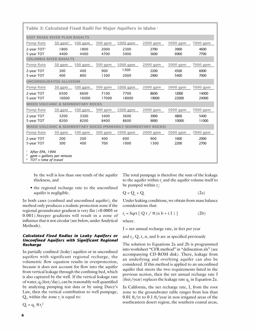
drawdown criteria to aquiferswith similar characteristics tothe aquifer to be protected,and (3) a compass to draw acircle with a radius aroundthe well(s) that equals thedistance criterion. Themethod does not explicitlyaccount for site-specificconditions, except that someassessment of theapplicability of theassumptions used indeveloping the distancecriterion to the site isrequired. Refer to Table 1for advantages anddisadvantages of thismethod.Under California’s DWSAP program, this method canonly be used for non-community water systems. It isthe simplest method, but also the least accurate method.To provide a conservative measure of protection, theprotection area typically ends up being relatively large.In most applications, an arbitrary fixed radius is chosenbased on transmissivity and pumping rate, therebyindirectly accounting for time of travel. Table 3identifies fixed radii for a number of different aquifertypes (in Idaho), where the radius is based on pumpingrate and transmissivity and depends on the time of travelrequired. The method allows identification of an interimprotective radius until more accurate wellheaddelineation methods can be used.

Calculated Fixed Radius (Cylinder Method)

The calculated fixed radius method (CFR) uses avolumetric flow equation to calculate a fixed radiusaround a well from which water will flow at a specifiedtime of travel (Figure 3). Because it involves solving asimple equation, it is also an example of a very simpleanalytical method. In the CFR method, the radius, ineffect, defines a circular time-of-travelisochrone around the well. The circle delimitsa cylinder within the aquifer that holds exactlythe amount of water that is pumped duringthe specified period. In other words, whatcomes out of the well must be equal to whatwas in the aquifer cylinder before (principle ofwater mass balance). Applying the principleof water mass balance, the equation forcalculating the fixed (cylinder) radius, fromwhich water comes within some time of travel,t, is:rt = Sqrt [ Q t / π n b ] (1)

where:Q = pumping capacity of well, in ft3/year

(note: ft3/year = gpm ⋅ 70,257)

t = time of travel, in years (2, 5, or 10 years for ZonesA, B5, and B10, respectively)

π = 3.1416

n = aquifer porosity, usually from 0.1 to 0.3 (10%–30%);where unknown, the California DWSAP specifies touse 20%

b = open interval or length of well screen, in feet; whereunknown, the California DWSAP specifies that b (infeet) is equal to 0.1 times the maximum pumping rate(in gpm)

rt = radius of zone, in feet, for time of travel t

The CFR method ignores the complexity ofgroundwater flow. Equation 1 is therefore only a coarseapproximation. It is most appropriate for a confinedaquifer with little vertical leakage from the overlyingconfining bed. It can also be used in unconfinedaquifers, if:

• the depth of the cone of depression generated

GeometricMethods

METHOD

Table 2: Estimated Work Hours, Expertise, & Overhead Costsfor Delineation 1

WORK HOURS LEVEL OF EXPERTISE 2 OVERHEAD COSTS

1, 21 to 10

AnalyticMethods

Hydrogeologicmapping

Computermodeling

1 After E.P.A., 19872 Key to levels of expertise: 1 = non-technical; 2 = junior hydrogeologist; 3 = mid-

level hydrogeologist/modeler; 4 = senior hydrogeologist/modeler

low

32 to 20 moderate

4 to 40 3 moderate to high

10 to 200 4 high

Figure 2: Delineation of wellhead protection area by fixed radiusmethod. (From EPA, 1994, Figure 4-4)

6

by the well is less than one-tenth of the aquiferthickness, and

• the regional recharge rate to the unconfinedaquifer is negligible.

In both cases (confined and unconfined aquifer), themethod only produces a realistic protection zone if theregional groundwater gradient is very flat (<0.0005 or0.001).Steeper gradients will result in a zone ofinfluence that is not circular (see below, under AnalyticalMethods).

Calculated Fixed Radius in Leaky Aquifers orUnconfined Aquifers with Significant RegionalRecharge

In partially confined (leaky) aquifers or in unconfinedaquifers with significant regional recharge, thevolumetric flow equation results in overprotection,because it does not account for flow into the aquiferfrom vertical leakage through the confining bed, whichis also captured by the well. If the vertical leakage rateof water, ql (feet/day), can be reasonably well quantifiedby analyzing pumping test data or by using Darcy’sLaw, then the vertical contribution to well pumpage,Ql, within the zone rt is equal to:

Ql = q1 π rt2

The total pumpage is therefore the sum of the leakageto the aquifer within rt and the aquifer volume itself tobe pumped within rt:

Q = Qa + Ql (2a)

Under leaking conditions, we obtain from mass balanceconsiderations that:

rt = Sqrt [ Q t / π (n b + t I ) ] (2b)

where:

I = net annual recharge rate, in feet per year

and rt, Q, t, n, and b are as specified previously

The solution to Equations 2a and 2b is programmedinto worksheet “CFR method” in “delineation.xls” (seeaccompanying CD-ROM disk). There, leakage froman underlying and overlying aquifer can also beconsidered. If this method is applied to an unconfinedaquifer that meets the two requirements listed in theprevious section, then the net annual recharge rate I(feet/year) replaces the leakage rate q1 in Equation 2a.

In California, the net recharge rate, I, from the rootzone to the groundwater table ranges from less than0.01 ft/yr to 0.1 ft/year in non-irrigated areas of thesoutheastern desert region, the southern coastal areas,

EAST SNAKE RIVER PLAIN BASALTS

Table 3: Calculated Fixed Radii for Major Aquifers in Idaho 1

Pump Rate 50 gpm2

20001800

1 After EPA, 19942 gpm = gallons per minute3 TOT = time of travel

27002-year TOT3

100 gpm 500 gpm 1000 gpm 2000 gpm 5000 gpm 7000 gpm

1800 2300 3900 460047004400 56005-year TOT 4400 5000 6900 7700

COLUMBIA RIVER BASALTS

Pump Rate 50 gpm

900300 22002-year TOT

100 gpm 500 gpm 1000 gpm 2000 gpm 5000 gpm 7000 gpm

400 4500 60001300400 29005-year TOT 800 2000 5400 7000

UNCONSOLIDATED ALLUVIUM

Pump Rate 50 gpm

71006500 86002-year TOT

100 gpm 500 gpm 1000 gpm 2000 gpm 5000 gpm 7000 gpm

6600 7700 12000 1400017000160005-year TOT 16000 18000 22000 24000

MIXED VOLCANIC & SEDIMENTARY ROCKS

Pump Rate 50 gpm

34003200 39002-year TOT

100 gpm 500 gpm 1000 gpm 2000 gpm 5000 gpm 7000 gpm

3300 3600 4800 540084008200 90005-year TOT 8200 8600 10000 11000

MIXED VOLCANIC & SEDIMENTARY ROCKS (PRIMARILY SEDIMENTARY ROCKS)

Pump Rate 50 gpm

400200 9002-year TOT

100 gpm 500 gpm 1000 gpm 2000 gpm 5000 gpm 7000 gpm

600 1600 2000700300 13005-year TOT 400 1000 2200 2700

1300

19000

200

7

and the Central Valley. In mountainous areas ofNorthern and Central California, recharge rates maybe as high as 1 ft/year. In areas with a large percentageof irrigated agriculture, the percolation of surplusirrigation water is the main source of recharge water;recharge in such areas ranges from 0.25 ft/yr to 1.5ft/yr, depending on the efficiency of the irrigationmethods used.

Computing Leakage Rate in a Leaky ConfinedAquifer

Leakage into a production aquifer (theaquifer from which a particular well drawswater) from an overlying or underlyingaquifer is a common situation. Thefollowing example illustrates how tocompute the leakage rate in such a situation.

Example: Two or more aquifers areseparated by a more or less well definedaquitard, through which flow is primarilyvertical. Determining leakage rate, ql (infeet/year), from one aquifer to another viaa confining aquitard unit can be achievedby using the principle of Darcy’s Law:

ql = Ql /A = 48.79 Kv i

where:

i = (houtside – hproduction) / b1

ql = quantity of leakage, in feet per year

Ql = total leakage, in ft3/year

A = cross-sectional area through whichleakage occurs, in ft2

Kv = vertical hydraulic conductivity ofthe confining unit, in gpd/ft2 (1 gpd/ft2 = 48.79 ft/year)

i = hydraulic gradient across theconfining unit

b1 = thickness of the confining unit, infeet

houtside = average head (water level) inthe overlying or underlying aquifer(above or below the productionaquifer), in feet

hproduction = average head (water level)in the production aquifer, in feet

Figure 4 illustrates two aquifersseparated by a layer of clayey silt. Theclayey-silty confining unit is 10 feetthick and has a hydraulic conductivityof 0.1 gpd/ft2. The difference in waterlevel between wells tapping the upper

and lower aquifers is 15 feet. The leakage rate is:

ql = 48.79 [ft3/gal ⋅ day/year] ⋅ 0.1 gpd/ft2 ⋅ 15 ft /10 ft = 7.33 ft/year

Assuming that, for example, protection zone A turnsout to have an area of 1 square mile (27.8784 millionsquare feet), the annual quantity leaking from thedeeper aquifer to the shallower one is:

Ql = 7.33 ft/year ⋅ (5280 ft)2 =204 million cubic feetper year ( = 2,900 gpm)

Figure 3: Delineation of wellhead protection area by cylinder method. (FromEPA, 1994, Figure 4-4)

Figure 4: Using Darcy’s law to calculate the quantity of leakage from oneaquifer to another. (From EPA, 1994, Figure 4-9)

8

This calculation clearly shows that the quantity ofleakage, either upward or downward, can be significant,even if the hydraulic conductivity of the confining unitis low.

Some authors have proposed using the time of travelacross a confining layer as one of several criteria fordifferentiating semiconfined aquifers from highlyconfined aquifers.Vertical time of travel across aconfining layer is:

tv = h1 ql / b1

where factors not defined above are:

tv = vertical time of travel (years) across theconfining layer

h1 = porosity of the confining unit

The required information comes from welllog interpretation and pumping tests of thewell or well field. Kreitler and Senger (1991)recommend a 40-year time of travel todifferentiate a semiconfined aquifer (TOT <40 years) from a confined aquifer (TOT >40years).

Additional Notes Regarding CFR

In order to prevent a gross underestimationof the radius rt of zones A, B5, and B10 (t =2, 5, or 10, respectively), the lowestreasonable leakage rate, ql, (or net rechargerate, I) should be used in these calculations.If the leakage (or recharge) rate is unknown,the effect of leakage (or recharge) should beneglected or more sophisticated tools shouldbe used for delineation.

In many cases, Q is not a constant value, butvaries with demand, build-out, etc. TheCalifornia DWSAP specifies that the pumpingcapacity, Q, of the well is to be used in theabove equations. The pumping capacity is themaximum rate at which the well can bepumped. Under certain circumstances, awater supplier may instead use the totalannual production of the well in the highestof the previous three to five years (in ft3/year)for calculations. Water suppliers areencouraged to consider future productionlevels if significant growth is expected tooccur in the service area.

Simplified Variable Shapes forSloping Aquifers: Modified CFR

As previously discussed, the assumption thatmost of the aquifer water contributing to awell originates from a cylindrical volume

around the well is only appropriate in the immediatevicinity of a pumping well (up to 50–100 feet from thewell), or if the regional aquifer gradient is negligible. Ifthe potentiometric surface (for confined aquifer) or thewater table (for unconfined aquifer) has a significantregional slope, then most of the contribution to thewell is from the upgradient area and only a small amountcomes from an area of limited size downgradient froma well (Figure 5). California DWSAP protection zonesA, B5, and B10 therefore have an asymmetric shapearound the well. As a preliminary assessment tool in

Figure 5: Groundwater flow paths to a pumping well with a capacityof 1,000 gpm in a 100 ft. thick aquifer with a hydraulic conductivityof 748 gpd/ft2 (100 ft/day). Regional groundwater flow is from rightto left. The ten-year time-of-travel (TOT) zone is demarcated by theouter beginning of the flow paths. The tips of the arrows along theflow paths demarcate the five-year TOT zone. This figure illustratesthe influence of the regional hydraulic gradient on the shape of thefive- and ten-year TOT and compares it to the equivalent shapeobtained from the calculated fixed radius (CFR) method for the 10-year TOT (circle). At very small slopes (< 0.05%), the shape of the twoTOT zones is approximately circular. The greater the regional slopeof the aquifer, the less circular the shape. Clearly, at slopes of 0.1%or larger, the cylinder method (circular protection area) yields a poorestimate of the actual wellhead protection area.

9

porous media aquifers (but not in fractured aquifers),DWSAP allows the use of a modified calculated fixedradius method (modified CFR). In the modified CFR,the sizes of the cylindrical protection zones are exactlythe same as in the CFR methods described above, butthe center of the cylinder is moved upgradient by halfthe length of the radius, Rt, of the cylinder. For example,if the radius of Zone A is determined to be 1000 ft, thecenter of Zone A is 500 ft (half of 1000 ft) upgradientfrom the well (Figure 6). Calculations to determinethe direction of groundwater flow must be submittedto DWSAP together with the computations for the sizeof the protection zones.

Other Simplified Variable Shapes for SlopingAquifers

Another simplified variable shapes approach takesadvantage of the fact that the size and shapeof protection zones will be very similar withinan area of a regional aquifer distinguished bya uniform gradient (similar direction andsimilar slope of the gradient throughout thearea) and similar aquifer properties (porosity,hydraulic conductivity). Once the size andshape of the protection zones has beendetermined for one well (using any numberof sophisticated tools), the same size and shapecan be applied to delineate the protectionzones of other wells in the area (Figure 7).However, the entire protection zone, not justthe well itself, must be inside the area withinwhich the aquifer gradient and aquiferproperties have been determined to beuniform.

If aquifer characteristics vary in the area inwhich the shapes are to be used, then differentcombinations of aquifer parameters andpumping rates are tested to determine a largeset of shapes. Tens or even hundreds ofcalculations may be required to establish“typical” shapes for dif ferent aquifercharacteristics and pumping rates. Thismethod requires that the necessarypreliminary work to define shapes has beencompleted. Delineation of a protection zoneor WHPA then only requires (1) enoughinformation about a well to determine whichshape “fits,” and (2) knowledge of the generaldirection of natural ground water flow toorient the shape if it has any asymmetry(Figure 7). Table 1 identifies relativeadvantages and disadvantages of this method.

In California, no statewide set of “shapes” hasbeen developed, due to the variety ofhydrogeologic settings within the state. Local

districts, communities, or groups of entities sharing aregional aquifer may consider developing a unified setof simplified variable shapes where local aquiferconditions allow (e.g., relatively uniform regionalhydraulic gradient and similar aquifer conditionsthroughout the area of interest). The set of variableshapes must reflect all important regional and localaquifer conditions. It would be applied to individualcommunity and non-community wells as a(recommended) minimum requirement for delineationof protection zones. Safety factors can be built in easily,by increasing the size of the shape by a given factor ordistance. Because the simplified variable shapes reflectactual aquifer conditions (hydraulic conductivity,regional aquifer gradient, etc.), this method generallyyields far more realistic protection zones than the CFRmethod.

Figure 6: Same as Figure 5, but here the circles indicate the protectionzones obtained from the California DWSAP modified CFR method. TheCFR method works best at some low to intermediate groundwater levelgradients (may vary by aquifer properties). At higher gradients it stillprovides a poor approximation of the protection zone actually needed.

10

Analytical Methods: Overview

Arbitrary radius, CFR, modified CFR, and other simpleshape methods represent only the most rudimentary“back-of-the-envelope” methods to delineateprotection zones or WHPAs. Those methods are eitherarbitrary (i.e., without any relation to the well andaquifer characteristics) or based on simple mass balanceconsiderations. Mass balance is indeed the mostimportant tool for protection zone delineation. Butbeyond the definition of simple cylindric shapes, wemust apply mass balance considerations and considerregional aquifer flow around the well. Flow in an aquiferis fundamentally governed by:

• Darcy’s law, which says that the flow rate isproportional to hydraulic conductivity and thehydraulic gradient, and inversely proportionalto porosity,

• the principle of mass conservation: what goes inmust come out or result in a change of waterstorage—much like a bank account,

• aquifer geometry, aquifer boundary conditions,recharge, pumping rates and pumping location,and historic circumstances (initial conditions).

Together, Darcy’s law and the “principle ofmass conservation” (or “principle ofcontinuity”) provide the basis for allgroundwater flow computations. They areexpressed in the groundwater flow equation,which applies to practically all groundwatersituations in porous media aquifers, and tomany situations of fractured rock aquifers. Allanalytical and numerical methods forprotection zone delineation are based on thisequation. Why is there not just one solution tothis equation? Because an important part ofsolving this equation mathematically is thehistorical water level condition. (Inmathematics, this is called the initialcondition.)

Another important part is the particulargeometry of the aquifer (the boundaryconditions), and the many different forms ofrecharge and pumping stresses distributedthroughout the aquifer (internal boundaryconditions). Each set of circumstances requiresa particular solution of the groundwater flowequation.

There are two ways to solve the flow equationwith all these conditions imposed on it: eitherthrough theoretical mathematical analysis,resulting in an analytical model (e.g., the Theisequation, which is commonly used to analyzepumping test results), or by computermodeling.

The many analytical models available in the literaturedescribe solutions to the groundwater flow equationthat were derived for specific idealized hydrogeologicsettings and well configurations, and for specific aquiferboundary conditions and other conditions, such aspartially penetrating wells, fully penetrating wells,confined aquifer, unconfined aquifer, multiple aquifers,leaky aquifer, etc. The mathematical complexity of someof these models challenges even the best mathematician.Regardless of complexity, though, all of the modelssimplify the aquifer into a more or less idealized simplegeometric shape. (See, for example, Figures 2, 8). Insome cases, an analytical model is satisfactory, but oftena computer model is preferred—for example, whenevaluating the effects of a complicated pumping pattern(e.g., Figure 9).

Both analytical and computer models for solving thegroundwater flow equation can be used to determinethe time of travel for delineating a wellhead protectionarea or protection zone. Again, the spectrum ofavailable tools in either category (analytical or computermodeling) ranges from the simple to the difficult,depending on the degree of information available andthe degree of accuracy desired.

Figure 7: Delineation of wellhead protection area by simplified shapesmethod. (From EPA, 1994, Figure 4-4)

11

If representative water level maps are available from adense network of pumping wells or observation wells,those maps, in conjunction with information aboutaquifer properties (hydraulic conductivity and porosity),can be used to estimate and delineate the areas withinwhich the time of travel (TOT) of water to a well is lessthan a given threshold (2 years, 5 years, 10 years).

But, in many cases, water table or potentiometric surfacedistribution are only known with limited accuracy,usually because individual wells are often sparselydistributed through an area, thousands of feet apart.Then, the first step in estimatingTOT is to come up with anestimated map of the water table orpotentiometric surface around thepumping well that reflects the coneof depression created by pumpingaround the well.

While the cone of depression(sometimes called zone of influence)is not the same as the recharge area,a good knowledge of its shape andsize is an important factor indelineating the recharge area andthe various TOT-based protectionareas within the recharge area.Computations of drawdown in thevicinity of the well (by analytical,semi-analytical, or computermethods) is therefore often anintegral part of determining theTOT-based protection zones.

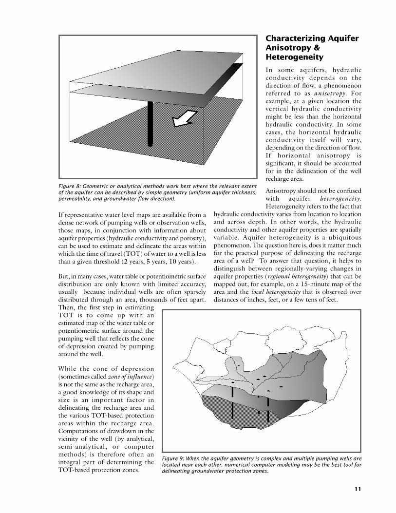
Characterizing AquiferAnisotropy &Heterogeneity

In some aquifers, hydraulicconductivity depends on thedirection of flow, a phenomenonreferred to as anisotropy. Forexample, at a given location thevertical hydraulic conductivitymight be less than the horizontalhydraulic conductivity. In somecases, the horizontal hydraulicconductivity itself will vary,depending on the direction of flow.If horizontal anisotropy issignificant, it should be accountedfor in the delineation of the wellrecharge area.

Anisotropy should not be confusedwith aquifer heterogeneity.Heterogeneity refers to the fact that

hydraulic conductivity varies from location to locationand across depth. In other words, the hydraulicconductivity and other aquifer properties are spatiallyvariable. Aquifer heterogeneity is a ubiquitousphenomenon. The question here is, does it matter muchfor the practical purpose of delineating the rechargearea of a well? To answer that question, it helps todistinguish between regionally-varying changes inaquifer properties (regional heterogeneity) that can bemapped out, for example, on a 15-minute map of thearea and the local heterogeneity that is observed overdistances of inches, feet, or a few tens of feet.

Figure 8: Geometric or analytical methods work best where the relevant extentof the aquifer can be described by simple geometry (uniform aquifer thickness,permeability, and groundwater flow direction).

Figure 9: When the aquifer geometry is complex and multiple pumping wells arelocated near each other, numerical computer modeling may be the best tool fordelineating groundwater protection zones.

12

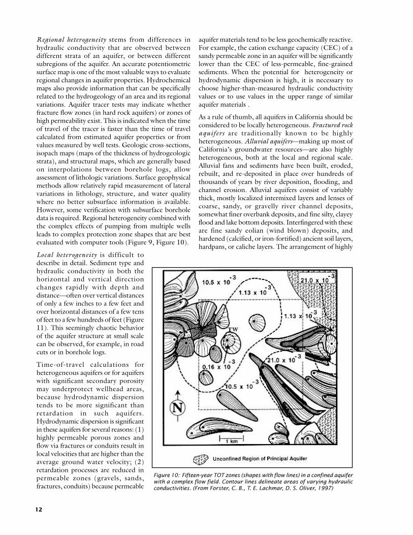
Regional heterogeneity stems from differences inhydraulic conductivity that are observed betweendifferent strata of an aquifer, or between differentsubregions of the aquifer. An accurate potentiometricsurface map is one of the most valuable ways to evaluateregional changes in aquifer properties. Hydrochemicalmaps also provide information that can be specificallyrelated to the hydrogeology of an area and its regionalvariations. Aquifer tracer tests may indicate whetherfracture flow zones (in hard rock aquifers) or zones ofhigh permeability exist. This is indicated when the timeof travel of the tracer is faster than the time of travelcalculated from estimated aquifer properties or fromvalues measured by well tests. Geologic cross-sections,isopach maps (maps of the thickness of hydrogeologicstrata), and structural maps, which are generally basedon interpolations between borehole logs, allowassessment of lithologic variations. Surface geophysicalmethods allow relatively rapid measurement of lateralvariations in lithology, structure, and water qualitywhere no better subsurface information is available.However, some verification with subsurface boreholedata is required. Regional heterogeneity combined withthe complex effects of pumping from multiple wellsleads to complex protection zone shapes that are bestevaluated with computer tools (Figure 9, Figure 10).

Local heterogeneity is difficult todescribe in detail. Sediment type andhydraulic conductivity in both thehorizontal and vertical directionchanges rapidly with depth anddistance—often over vertical distancesof only a few inches to a few feet andover horizontal distances of a few tensof feet to a few hundreds of feet (Figure11). This seemingly chaotic behaviorof the aquifer structure at small scalecan be observed, for example, in roadcuts or in borehole logs.

Time-of-travel calculations forheterogeneous aquifers or for aquiferswith significant secondary porositymay underprotect wellhead areas,because hydrodynamic dispersiontends to be more significant thanretardation in such aquifers.Hydrodynamic dispersion is significantin these aquifers for several reasons: (1)highly permeable porous zones andflow via fractures or conduits result inlocal velocities that are higher than theaverage ground water velocity; (2)retardation processes are reduced inpermeable zones (gravels, sands,fractures, conduits) because permeable

aquifer materials tend to be less geochemically reactive.For example, the cation exchange capacity (CEC) of asandy permeable zone in an aquifer will be significantlylower than the CEC of less-permeable, fine-grainedsediments. When the potential for heterogeneity orhydrodynamic dispersion is high, it is necessary tochoose higher-than-measured hydraulic conductivityvalues or to use values in the upper range of similaraquifer materials .

As a rule of thumb, all aquifers in California should beconsidered to be locally heterogeneous. Fractured rockaquifers are traditionally known to be highlyheterogeneous. Alluvial aquifers—making up most ofCalifornia’s groundwater resources—are also highlyheterogeneous, both at the local and regional scale.Alluvial fans and sediments have been built, eroded,rebuilt, and re-deposited in place over hundreds ofthousands of years by river deposition, flooding, andchannel erosion. Alluvial aquifers consist of variablythick, mostly localized intermixed layers and lenses ofcoarse, sandy, or gravelly river channel deposits,somewhat finer overbank deposits, and fine silty, clayeyflood and lake bottom deposits. Interfingered with theseare fine sandy eolian (wind blown) deposits, andhardened (calcified, or iron-fortified) ancient soil layers,hardpans, or caliche layers. The arrangement of highly

Figure 10: Fifteen-year TOT zones (shapes with flow lines) in a confined aquiferwith a complex flow field. Contour lines delineate areas of varying hydraulicconductivities. (From Forster, C. B., T. E. Lachmar, D. S. Oliver, 1997)

13

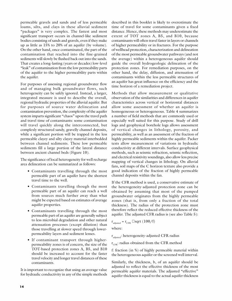
Figure 11: Illustration of aquifer heterogeneity at various scales. The top photo is an aerial photograph of mountain valleyand basin aquifers. The remaining photographs are of vertical (or almost vertical) cross-sections through geologic materialthat can serve as a groundwater reservoir. The width of the cross-sections vary from several kilometers (top) to less thanan inch (bottom), yet all exhibit patterns of heterogeneity.

14

permeable gravels and sands and of less permeableloams, silts, and clays in these alluvial sediment“packages” is very complex. The fastest and mostsignificant transport occurs in channel-like sedimentbodies consisting of sands and gravels, even if they makeup as little as 15% to 20% of an aquifer (by volume).On the other hand, once contaminated, the part of thecontamination that reached into the fine-grainedsediments will slowly be flushed back out into the sands.That creates a long-lasting (years or decades) low-level“leak” of contamination from the low permeability partsof the aquifer to the higher permeability parts withinthe aquifer.

For purposes of assessing regional groundwater flowand of managing bulk groundwater flows, suchheterogeneity can be safely ignored. Instead, a larger,integrated measure is used to describe the overall,regional hydraulic properties of the alluvial aquifer. Butfor purposes of source water delineation andcontamination prevention, the complexity of the aquifersystem imparts significant “chaos” upon the travel pathand travel time of contaminants: some contaminationwill travel quickly along the interconnected, butcomplexly structured sandy, gravelly channel deposits,while a significant portion will be trapped in the lesspermeable clayey and silty clayey material interbeddedbetween channel sediments. These low permeablesediments fill a large portion of the lateral distancebetween ancient channel beds (Figure 10).

The significance of local heterogeneity for well rechargearea delineation can be summarized as follows:

• Contaminants travelling through the mostpermeable part of an aquifer have the shortesttravel time to the well.

• Contaminants travelling though the mostpermeable part of an aquifer can reach a wellfrom sources much further away than whatmight be expected based on estimates of averageaquifer properties.

• Contaminants travelling through the mostpermeable part of an aquifer are generally subjectto less microbial degradation and other naturalattenuation processes (except dilution) thanthose travelling at slower speed through lower-permeability layers and sediment lenses.

• If contaminant transport through higher-permeability zones is of concern, the size of theTOT-based protection zones A, B5, and B10should be increased to account for the fastertravel velocity and longer travel distances of thesecontaminants.

It is important to recognize that using an average valuefor hydraulic conductivity in any of the simple methods

described in this booklet is likely to overestimate thetime of travel for some contaminants given a fixeddistance. Hence, these methods may underestimate theextent of TOT zones A, B5, and B10, becausecontaminants will often travel faster in layers or channelsof higher permeability or in fractures. For the purposeof wellhead protection, characterization and delineationof the most permeable groundwater pathways (and notthe average) within a heterogeneous aquifer shouldguide the overall hydrogeologic delineation of theprotection zones. For remediation purposes, on theother hand, the delay, diffusion, and attenuation ofcontaminants within the less permeable structures ofan aquifer has great influence on the efficiency and thetime horizon of a remediation project.

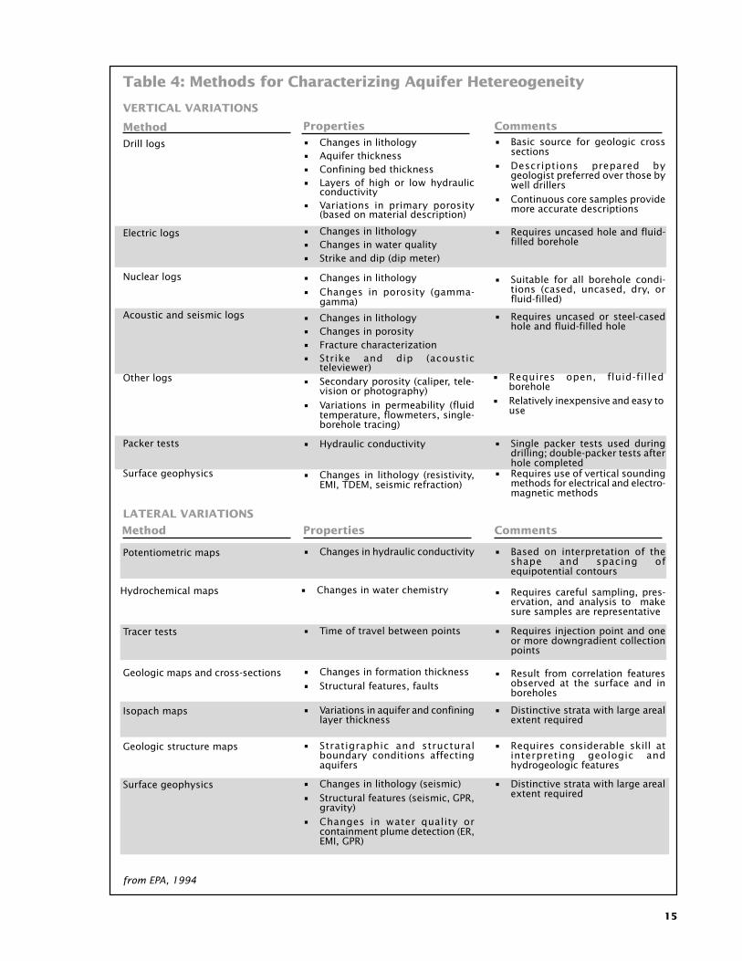
Methods that allow measurement or qualitativeobservation of the similarities and differences in aquifercharacteristics across vertical or horizontal distancesallow some assessment of whether an aquifer ishomogeneous or heterogeneous. Table 4 summarizesa number of field methods that are commonly used orespecially well suited for this purpose. Study of drilllogs and geophysical borehole logs allows assessmentof vertical changes in lithology, porosity, andpermeability, as well as an assessment of the fraction ofhighly permeable sediments within the aquifer. Packertests allow measurement of variations in hydraulicconductivity at different intervals. Surface geophysicalmethods, such as seismic refraction, seismic reflection,and electrical resistivity soundings, also allow less precisemapping of vertical changes in lithology. On alluvialfans, soil maps of the C horizon texture also provide agood indication of the fraction of highly permeablechannel deposits within the fan.

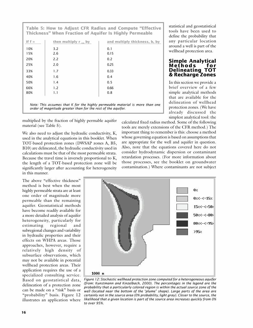
If the CFR method is used, a conservative estimate ofthe heterogeneity-adjusted protection zone can beobtained by assuming that most of the pumpedgroundwater originates from the highly permeablezones (that is, from only a fraction of the totalthickness). The radius of the protection zone musttherefore reflect the reduced effective thickness of theaquifer. The adjusted CFR radius is (see also Table 5):

radjusted = rCFR ⋅ sqrt (100/f)

where:

radjusted: heterogeneity-adjusted CFR radius

rCFR: radius obtained from the CFR method

f: fraction (in %) of highly permeable material withinthe heterogeneous aquifer or the screened well interval.

Similarly, the thickness, b, of an aquifer should beadjusted to reflect the effective thickness of the mostpermeable aquifer materials. The adjusted “effective”aquifer thickness is equal to the actual aquifer thickness

15

Comments

Table 4: Methods for Characterizing Aquifer Hetereogeneity

Method

Drill logs

VERTICAL VARIATIONS

Properties• Basic source for geologic cross

sections• Descriptions prepared by

geologist preferred over those bywell drillers

• Continuous core samples providemore accurate descriptions

• Changes in lithology• Aquifer thickness• Confining bed thickness• Layers of high or low hydraulic

conductivity• Variations in primary porosity

(based on material description)

Electric logs • Requires uncased hole and fluid-filled borehole

• Changes in lithology• Changes in water quality• Strike and dip (dip meter)

Nuclear logs • Suitable for all borehole condi-tions (cased, uncased, dry, orfluid-filled)

• Changes in lithology• Changes in porosity (gamma-

gamma)

CommentsMethod

Potentiometric maps

LATERAL VARIATIONS

Properties

• Based on interpretation of theshape and spacing ofequipotential contours

• Changes in hydraulic conductivity

Hydrochemical maps • Requires careful sampling, pres-ervation, and analysis to makesure samples are representative

• Changes in water chemistry

from EPA, 1994

Acoustic and seismic logs • Requires uncased or steel-casedhole and fluid-filled hole

• Changes in lithology• Changes in porosity• Fracture characterization• Strike and dip (acoustic

televiewer)Other logs • Requires open, fluid-filled

borehole• Relatively inexpensive and easy to

use

• Secondary porosity (caliper, tele-vision or photography)

• Variations in permeability (fluidtemperature, flowmeters, single-borehole tracing)

Packer tests • Single packer tests used duringdrilling; double-packer tests afterhole completed

• Hydraulic conductivity

Surface geophysics • Requires use of vertical soundingmethods for electrical and electro-magnetic methods

• Changes in lithology (resistivity,EMI, TDEM, seismic refraction)

Tracer tests • Requires injection point and oneor more downgradient collectionpoints

• Time of travel between points

Geologic maps and cross-sections • Result from correlation featuresobserved at the surface and inboreholes

• Changes in formation thickness• Structural features, faults

Isopach maps • Distinctive strata with large arealextent required

• Variations in aquifer and confininglayer thickness

Geologic structure maps • Requires considerable skill atinterpreting geologic andhydrogeologic features

• Stratigraphic and structuralboundary conditions affectingaquifers

Surface geophysics • Distinctive strata with large arealextent required

• Changes in lithology (seismic)• Structural features (seismic, GPR,

gravity)• Changes in water quality or

containment plume detection (ER,EMI, GPR)

16

statistical and geostatisticaltools have been used todefine the probability thatany particular locationaround a well is part of thewellhead protection area.

Simple AnalyticalMethods forDelineating TOT& Recharge Zones

In this section we provide abrief overview of a fewsimple analytical methodsthat are available for thedelineation of wellheadprotection zones. (We havealready discussed thesimplest analytical tool: the

calculated fixed radius method. Some of the followingtools are merely extensions of the CFR method.) Theimportant thing to remember is this: choose a methodwhose governing equation is based on assumptions thatare appropriate for the well and aquifer in question.Also, note that the equations covered here do notconsider hydrodynamic dispersion or contaminantretardation processes. (For more information aboutthose processes, see the booklet on groundwatercontamination.) Where contaminants are not subject

multiplied by the fraction of highly permable aquifermaterial (see Table 5).

We also need to adjust the hydraulic conductivity, K,used in the analytical equations in this booklet. WhenTOT-based protection zones (DWSAP zones A, B5,B10) are delineated, the hydraulic conductivity used incalculations must be that of the most permeable strata.Because the travel time is inversely proportional to K,the length of a TOT-based protection zone will besignificantly larger after accounting for heterogeneityin this manner.

The above “effective thickness”method is best when the mosthighly permeable strata are at leastone order of magnitude morepermeable than the remainingaquifer. Geostatistical methodshave become readily available fora more detailed analysis of aquiferheterogeneity, particularly forestimating regional andsubregional changes and variabilityin hydraulic properties and theireffects on WHPA areas. Thoseapproaches, however, require arelatively high density ofsubsurface observations, whichmay not be available in potentialwellhead protection areas. Theirapplication requires the use of aspecialized consulting service.Based on geostatistical data,delineation of a protection zonecan be made on a “risk” basis or“probability” basis. Figure 12illustrates an application where

10%

Table 5: How to Adjust CFR Radius and Compute “EffectiveThickness” When Fraction of Aquifer Is Highly Permeable

then multiply r CFR by and multiply thickness, b, by

3.2

Note: This assumes that K for the highly permeable material is more than oneorder of magnitude greater than for the rest of the aquifer.

0.1

If f =

15% 2.6 0.15

2.2 0.2

25% 2.0 0.25

33% 1.7 0.33

40% 1.6 0.4

50% 1.4 0.5

66% 1.2 0.6680% 1.1 0.8

20%

Figure 12: Stochastic wellhead protection zone computed for a heterogeneous aquifer(from: Kunstmann and Kinzelbach, 2000). The percentages in the legend are theprobability that a particularly colored region is within the actual source zone of thewell (located near the bottom of the “plume” shape). Large parts of the area arecertainly not in the source area (0% probability, light gray). Closer to the source, thelikelihood that a given location is part of the source area increases quickly from 0%to over 95%.

17

to attenuation (for example, salts, chlorides, nitrates,MTBE), calculating the time of travel should provide areasonably accurate delineation of the area at risk.

Delineating Protection Zone for a Well in anAquifer with Uniform Sloping Gradient

The effect of a uniform slope on the shape of the 5-year and 10-year protection zones is demonstrated inFigures 5 and 6. The shape of these protection zonesis almost circular in an aquifer with very lowslopes (< 0.05%), but the shape becomeslonger and narrower at steeper slopes andmost of the time-of-travel (TOT) zone willbe upgradient of the well and not around thewell. When the slope is significant (0.1% orgreater), it should be accounted for in thedelineation of the TOT zones.

The so-called uniform flow equation has beenwidely used for the delineation of wellheadprotection areas and recharge zones where asloping regional hydraulic gradient creates anasymmetrical cone of depression (Figure 13a).The recharge zone (zone of contribution) isdefined using two equations originallydeveloped in 1930 by Forchheimer:

xlimit = 1,440 ⋅ Q / (2π K b i ) (3)

and

ylimit = 1,440 ⋅ Q / K b i (4)

where (see also Figure 13b):

xlimit: furthest point downgradient from thewell within the cone of depression, ft

ylimit: maximum width of the upgradientrecharge zone, ft

Q: average pump discharge, gpm

K: hydraulic conductivity, gpd/ft2

b: thickness of the aquifer, ft (the well isassumed to penetrate the entire aquifer)

i: average regional gradient of thegroundwater level (or potentiometric surface)

These simple equations define thedowngradient flow boundary, xlimit , and themaximum width, ylimit, of the upgradientrecharge zone, respectively (Figure 13b). Buthow would this method be used fordelineation? Equations 3 and 4 provide thewidth of the recharge area and the downslopeextent of the cone of depression. In theupgradient direction, TOT zones and thecomplete recharge area can be determined byother means:

1. TOT estimates can be made (discussed in thesections that follow) to draw an approximateTOT contour within the shape delineated byxlimit and ylimit and the upgradient time-of-travelisochrone (Figure 13b). This alternative wouldused in California for delineating zones A, B5,and B10.

2. The entire recharge area can be delineated byextending the flowlines that mark the

Figure 13: Flow to a well in a uniformly sloping potentiometric surface:(a) cross-section (upper), and (b) plan view (lower). (Modified from EPA,1994, Figure 4-10)

18

boundaries of ylimit all the way back (“uphill”)to a ground water divide or other aquiferboundary.

The uniform flow equation applies, strictlyspeaking, only to confined aquifers. But, as inthe CFR method, the above equations can alsobe used for unconfined aquifers, using thesaturated thickness of the aquifer, provided thatdrawdown is less than 10 percent of thesaturated thickness of the aquifer. The aboveequations do not account for leakage. Byneglecting leakage, this model will define largerTOT protection areas than are necessary.

Delineating TOT Zones within UniformRegional Gradient

The time of travel (TOT) from a distance x to the wellis computed by considering the groundwater velocitywithin that area. Groundwater velocity estimates areobtained by applying Darcy’s law, which describes thegroundwater velocity as a function of the hydraulicconductivity, porosity, and groundwater hydraulicgradient:

v = 48.79 K i / n (5)

where:v = average interstitial (linear) velocity, ft/yrK = horizontal hydraulic conductivity, gpd/ft2

i = approximate horizontal or radial hydraulic gradient,averaged over the area of interest, ft/ftn = aquifer porosity; usually from 0.1 to 0.3 (10%–30%); where unknown, the California DWSAP specifiesto use 20%

If the aquifer is relatively homogeneous and the slopeof the hydraulic gradient is uniform, then the velocity(from Equation 5) is computed after using apotentiometric map of the aquifer to measure thehydraulic gradient. If K and n values are not available,preliminary estimates of K and n can be obtained basedon the type of aquifer material. Once average velocityhas been computed with Equation 5, the distance thatgroundwater travels during a given time (e.g., 2 years,5 years, 10 years) is calculated as follows:

d = t v = 48.79 t K i / n (6)where:d = the distance, in feet, that water travels during tyears

v = average linear (pore) velocity, ft/yr

t = specified time of travel, years

Vice versa, the time, in years, needed for groundwaterto travel a distance d, in feet, between two points wherethe potentiometric slope, i, is uniform can be calculated

by rearranging Equation 6:

t = d / v = d n / (48.79 K i) (7)

Recharge Zone for Negligible RegionalGradient, Uniform Recharge

When the regional gradient is very low (< 0.0005 or0.001) and an aquifer receives either uniform rechargethrough the unsaturated zone (unconfined aquifer),through the upper or lower confining aquitards(confined aquifer), or through overburden (confinedand semi-confined aquifers), the recharge area to thewell is approximately of circular shape. The extent ofthat recharge area can be determined from simple massbalance: in the long term (that is, once the system hasreached steady-state), the discharge Q from theproduction well will equal the average recharge orleakage into the aquifer within that circular rechargearea. In an unconfined aquifer, the total recharge intothe recharge area is equal to the recharge rate, I, timesthe area of the circle delineating the recharge area:

Q = I π r2 (8)

where:

Q = annual pumpage, ft3/yr

r = radius of the recharge area, ft

I = infiltration, ft/yr

In a confined aquifer, the leakage into the aquifer isequal to the vertical hydraulic conductivity of theconfining layer, Kv, multiplied by the average pressuregradient across the confining layer and multiplied bythe recharge area:

Q = 48.79 ⋅ Kv i π r2 (9)

where:Q = annual pumpage, ft3/yrKv = vertical hydraulic conductivity in the confiningunit, gpd/ft2

i = average pressure gradient across the confining unitr = radius of the recharge area, ftSuggested Kv values for silt and clay (in the confininglayer) are on the order of 0.01 gpd/ft2. A spreadsheetfor computing the radius of recharge (delineation.xls)is included on the accompanying CD-ROM.This scenario is essentially identical to the CFR method,except that Equations 8 and 9 establish the entirerecharge area for a well and not just a zone with a fixedtime of travel (Equation 2). Also, note that Equation 2provides the distance from the well, given a specifiedtime of travel. To calculate the time of travel from agiven distance, r, to the well, we rearrange Equation 2and obtain:

t = πr2 b n / [70,258 x Q – π r2 (q1 + q2) (10)

19

where:

t: time of travel, years

r: distance from the well for which time of travel isbeing computed, ft

b: thickness of the aquifer, ft (assumed to be the sameas length of well screen)

n: porosity of the aquifer

Q: pumping rate at the well, gpm

q1: recharge rate from the unsaturated zone or leakagerate from the upper confining layer, ft/yr

q2: recharge rate from the lower confining layer, ft/yr

Like the CFR method, Equation 10 applies to confined,leaky confined, or unconfined aquifers. However, it canbe used for unconfined aquifers only if the totaldrawdown at the pumping well does not exceed 10%of the aquifer thickness. If total drawdown exceeds 10%,vertical flow near the well affects the travel time andEquation 10 does not apply.

Note that instead of using Equation 10, one couldcompute the TOT by (1) dividing the pathway to awell into segments each of which has approximatelyuniform potentiometric slope, (2) applying Equation7 to each segment, and then (3) adding up theindividual travel times.

The following example illlustrates how to calculate thevelocity and time of travel for a chemical contaminantin an aquifer with straight (uniform) slope throughoutthe area of interest (and negligible cone of depression,negligible heterogeneity).

Example: A liquid substance containing chloride spillsand leaks into the ground. The liquid waste infiltratesthrough the unsaturated zone and quickly reaches awater table aquifer that consists of sand and gravel witha hydraulic conductivity of 2,000 gpd/ft2 and aneffective porosity of 20%. The water level in a well atthe spill lies at an altitude of 1,525 feet and, at a wellone mile (5,280 feet) directly downgradient, is at 1,515feet. The potentiometric slope, i, is therefore 10 feetper 5,280 feet. The velocity of the water and thecontaminant, and the time it will take for the chlorideto contaminate the second well, can be determined fromEquations 7 and 9:

v = 48.79 ⋅ (2,000 gpd/ft2) ⋅ (10 ft / 5,280 ft) / 0.20= 924 ft/yr

t = 5,280 ft / (924 ft/year) = 5.7 years

The five year time-of-travel (TOT) zone is at thefollowing distance from the downgradient well(Equation 8):

d = 924 ft/year ⋅ 5 years = 4,620 feet

The spill is therefore outside the 5-year zone.

Note: 1 gpd/ft2 = 48.79 ft/year

Significant Cone of Depression Within aSloping Regional Potentiometric Surface

In most practical scenarios, when computing time oftravel, the regional groundwater table gradient cannotbe neglected (Figure 5). In those cases, the cone ofdepression will be asymmetric, with drawdownextending farther upgradient than downgradient. Anequation that accounts for the actual conical shape ofthe cone of depression within the regional groundwaterflow field is given by Kreitler and Senger (1991). Theequation allows us to compute the travel time from apoint x directly upgradient from the well to the wellitself:

tX = n / K i [ rX – Z ln {1+ rX/Z} (11)

where:

Z = Q / 2 π K b i

tX = time of travel from point x to a pumping well, inyears

n = porosity

rX = distance, in feet, over which groundwater travelsin tX; rX is positive (+) if the point is upgradient, andnegative (–) if downgradient

Q = pumping discharge, ft3/yr; (note: Q in ft3/yr =70,258 ⋅ Q in gpm)

K = hydraulic conductivity, ft/yr; (note: K in ft/yr =48.79 ⋅ K in gpd/ft2)

b = aquifer thickness, feet (complete well penetrationis assumed)

i = hydraulic gradient, ft/ft

The above equation computes travel time to the centerof the well and assumes that the well radius is smallrelative to the distance rx (<5%). Calculation of distancefor a specific time of travel requires trial-and-errorcalculations, using different values for distances, untilthe equation yields the desired time of travel. This canbe done easily using a computer spreadsheet. (Equation11 is implemented in the spreadsheet “delineation.xls”,included on the accompanying CD-ROM disk.)

Equation 11 is used after the recharge area has beendelineated around a well located within a uniformregional hydraulic gradient. The main weaknesses ofthis equation are:

• It only provides distance for time of travel alonga line through the pumping well and parallel to

20

the regional hydraulic gradient (i.e., one pointupgradient). Where equipotential lines on apotentiometric map are not straight lines, thiswould be the shortest flow line upgradient.

• It does not take into account recharge from thesurface in unconfined aquifers or vertical leakageinto semiconfined aquifers.

Kreiger and Senger (1991) recommend pathline tracingmodels such as WHPA and GWPATH as the bestmethod for calculating time of travel for confinedaquifers with regionally sloping potentiometric surfaces,because those models actually are able to define TOTcontours.

Hydrogeologic Mapping & Analysis

Hydrogeologic mapping provides a valuablecomplement to the simpler methods for delineatingprotection zones or wellhead protection areas. Inaddition, it is a necessary precursor to more complexnumerical modeling of ground water flow usingcomputers. Figure 14 illustrates WHPA delineationusing geologic contacts and ground water divides asthe key elements of hydrogeologic mapping.Potentiometric maps and methods for measuringaquifer parameters are also essential parts ofhydrogeologic mapping.

Hydrogeologic mapping and analysis should be doneonly by experienced, professional groundwaterspecialists. The purpose of this booklet is to providegeneral conceptual guidance on this technique for thosepreparing, planning, managing,subcontracting, or reviewing work related todelineation of protection zones. More detailedinformation about the method can be foundin some of the references listed at the end ofthis booklet.

Hydrogeologic mapping requires thesystematic and integrated appraisal of soils,geomorphology, geology, hydrology(including meteorologic aspects),geochemistry, and water chemistry as theyaffect the occurrence, flow, and quality ofground water.

A brief discussion of the significance of theseelements follows.

Soils & Geomorphology

The character and distribution of soils andlandforms are major considerations inhydrogeologic mapping. This is especially truefor lands within and adjacent to California’smountain ranges. Unconfined aquifers

develop in unconsolidated materials and lie relativelynear the land surface. In such settings, the water tablegenerally follows the land surface, although with moresubdued relief. Recharge areas are generally located inupland areas, and ground water divides tend to coincidewith surface watershed boundaries.The narrow valley bottoms and floodplains withinCalifornia’s mountainous regions that feature perennialstreams (primarily in Northern California) representgroundwater discharge areas (i.e., groundwaterdischarges into streams and other surface water bodies).As these streams and rivers enter the larger Californiavalleys and basins, they become a major source ofgroundwater recharge.In California’s rangelands and uplands, soils andtopography determine how much precipitationinfiltrates into the ground to recharge groundwater,and how much runs off to enter surface streams. Highlypermeable soils and flat topography favor infiltration;less permeable soils and steep slopes promote surfacerunoff.In the larger basins and valleys, which havepredominantly flat topography, factors other than soiltype are the primary controls on recharge rates andgroundwater discharge. One such factor is land use.We discuss land use in more detail later in this booklet.

Geology

Geology provides the physical framework for the flowof ground water. Porosity (primary and secondary),storage coefficient, and permeability (hydraulicconductivity) are largely a function of the geologic

Figure 14: Illustration of the concept of recharge area (primaryrecharge area) and source area (secondary recharge area). (FromCalifornia DWSAP, Figure 6-2)

21

materials present. Stratigraphy (the relationshipsbetween layered geologic materials) affects local andregional ground water flow by the distribution of strataof relatively higher and lower permeability. It definesthe sequence of aquifers, aquitards, and aquicludes aswell as their geographic extent, thickness, dip (angle oftilt) and strike (direction perpendicular to direction oftilt). In fractured rocks and consolidated materials,structural features such as folds or fractures—remnantsof ancient or recent tectonic processes—can block orchange the direction of groundwater flowing throughnearby horizontal sediments. Displacement ofsediments by faulting can provide zones of increasedpermeability, as a result of fracturing. It can just as easilycreate aquifer boundaries. These may occur, forexample, where impermeable strata block the flow ofwater through permeable strata. Secondary fractureporosity results primarily from tectonic stresses.

Hydrology

Although the focus of hydrogeologic mapping is ongroundwater, the occurrence and flow of groundwatermust be understood in the context of the largerhydrologic cycle, which includes atmospheric water,water in the vadose (unsaturated) zone, and surfacewater. This is especially true of unconfined aquifers,which are closely connected to the hydrologic cycle.

It is often useful to prepare a regional groundwaterbalance at the onset of a groundwaterproject. The overall groundwater budgetprovides a framework for the conceptualunderstanding of groundwater flowwithin the area of interest.

For a typical California groundwaterbasin, the major components of thehydrologic balance include: effectiveprecipitation, irrigation applications, cropwater demands (evapotranspiration),municipal and industrial water demands,surface water imports and exports, surfacewater inflows and outflows into the areaof interest, pumping demands, averagerecharge from precipitation and irrigationto groundwater, intentional recharge,recharge from rivers and canals, andgroundwater discharge to rivers.Examples of a hydrologic balance areshown in Figure 15 and Figure 16. The“California Water Plan Update” (DWRBulletin 160-98) contains an overallsketch of the water balance within thestate’s major regions.

Mapping of potentiometric surfaces isanother important part of the hydrologiccharacterization. For the purposes of

WHPA delineation, confined aquifers that are distantfrom their areas of surface recharge can be consideredto be semi-isolated from the hydrologic cycle, providedthat they are highly confined. This may greatly simplifythe analysis of the groundwater flow system.

Hydrochemistry

Data on water quality can provide valuable insights intothe hydrogeologic system. A number of hydrochemicalindicators are useful for assessing the presence anddegree of confinement of an aquifer. The geochemicalcharacteristics of the aquifer matrix and factors such aspH and redox potential (Eh) and aquifer microbiologyare especially important if the potential for attenuationof contaminants is being considered in the WHPAdelineation process.

Land use. Land use is a major component indetermining aquifer recharge and groundwaterpumping requirements. The largest pumpers ofgroundwater in California are cities and agriculturalusers. Knowing the urban and agricultural waterrequirements for an area, and the degree to which thoserequirements are met by surface water deliveries versusgroundwater pumping, greatly helps us to understandthe hydrologic balance of a groundwater basin. Mostimportantly, while pumping discharge from aquifers isa critical component of the groundwater budget, fewrecords of actual pumpage typically exist in California.

Figure 15: Water balance for a 550,000 acre groundwater basin on thesoutheast side of the semi-arid San Joaquin Valley, California. Numbersindicate annual fluxes of water in thousand acre-feet.

22

Groundwater pumpage must therefore be inferred frompower records (electricity or fuel consumption of agwell pumps is a significant portion of rural powerconsumption) or by difference between water demands(ag or urban) and surface water deliveries. The latter isthe preferred method when surface water deliveries andconsumptive use (for evapotranspiration) are wellknown.

Cities and agriculture are not only dominant users ofgroundwater, they also can be significant rechargers ofgroundwater. Many cities in central and southernCalifornia recharge their groundwater by dischargingtreated, secondary wastewater effluent into infiltrationbasins. Some cities also have built basins specifically forstoring surface water deliveries or for storing stormwaterrunoff; those basins also recharge groundwater aquifers.

Most of California’s agriculture relies on irrigation.Even the most efficient irrigation system will requiresome water leaching, leading to significant groundwaterrecharge from irrigation.

In municipal areas and in low-elevation, irrigatedagricultural areas throughout California, recharge ofgroundwater by precipitation is almost negligible whencompared to intentional (basin) recharge and to therecharge of groundwater by crop irrigation.

Numerical ComputerModeling

Where the aquifer geometry cannot bedescribed by a simple conceptual model(e.g., Figure 8), it is advantageous toexplicitly account for the complex aquifergeometry and for the complex historyof stresses that have been imposed on anaquifer (e.g., Figure 9). For that,computer models based on numericalmethods have become very popular.They solve the same fundamentalequation(s) as analytical models—andtherefore involve no more and no less“wizardry” than analytical models. Butunlike analytical models, computermodels can deal with very complex, non-ideal boundary conditions, pumping welldistributions, spatially non-uniformaquifer properties, etc. While not aperfect replica of the “real” aquifer, anumerical computer model allows amuch better and more truthfulrepresentation of the complexarchitecture and workings of an aquiferthan does an analytical model. In acomputer model, aquifers can havecomplex shapes, be of variable thickness,be only partially confined, or have aquifer

properties that vary spatially. Complex pumpage orrecharge patterns that vary over time and space canalso be modeled (Figure 17).

As with most other computer software, groundwatermodeling software is advancing at a rapid pace. Manydifferent kinds of groundwater modeling programs areavailable. The strict division between “analyticalmodels” and “computer models” has been blurred withthe introduction of computer software that utilizesanalytical models both to analyze graphically and toillustrate (e.g., wellhead protection areas displayeddirectly on a computer). Another example of ananalytical tool implemented on the computer is thespreadsheet “delineation.xls” (see accompanying CD-ROM disk). Computer software based exclusively onanalytical methods (i.e., mathematical solutions) arecommon for the analysis of aquifer test data, but alsofor the delineation of wellhead protection areas. Becauseof their generally easy-to-use PC Windows® interface,such software programs often are a potentially low-costalternative to more complex computer models.

What has traditionally been referred to as “computermodels” are so-called numerical methods or numericalcomputer models (as opposed to analytical methods oranalytically-based computer models). Numericaltechniques allow the computer modeler to design

Figure 16: Water balance for a groundwater basin on the west side of theSan Joaquin Valley, California. (Modified from Belitz and Phillips, 1995)

23

complex “virtual” copies of a real aquifer by discretizingthe aquifer into small boxes (usually referred to as“cells”) of variable size and shape, depending on theparticular numerical method (Figure 17). The principleis the same as that used for many other computersoftware applications that provide a virtual view of theworld (in two or three dimensions), be it a flight-simulator game, a virtual garden design program forthe home gardener, or professional engineering designsoftware.

The discretization allows the aquifer to have any desiredthree-dimensional shape. Rivers, lakes, streams (all ofwhich are typically linked to groundwater), fields(recharge from irrigation), wells, and contaminantsources can be implemented in arbitrary configurationsby assigning certain cells to represent these sinks orsources of water and contaminants. Because each smallcell can be assigned different aquifer properties, multipleaquifer layers and regional or even local differences(heterogeneities) in aquifer properties within eachaquifer can be implemented by assigning the appropriatenumbers to the individual cells. The accuracy and detailwith which this virtual aquifer represents reality islimited only by the number of cells that the numericalmodel can contain and by the geologic and hydrologicknowledge available to provide the appropriateproperties and sink-source strengths to the individualcells representing the aquifer, aquitards, aquiferboundaries, rivers, wells, fields, etc.

Numerical aquifer models currently developed by thehydrogeologic consulting industry contain from severalthousand to over 1,000,000 cells.

A lower number of cells (1,000 to 100,000) is typicallyused in site studies or in regional applications wherelocal heterogeneity of aquifer properties can be ignored.A relatively small number of cells may also beappropriate if the model is only two-dimensional (i.e.,representing only the horizontal flow processes of anaquifer).

A higher number of cells (> 100,000) is needed if localheterogeneities are modeled in significant detail or ifthe region to be modelled is very large and has acomplex three-dimensional shape. Numerical modelersrefer to these cells either as finite difference cells or finiteelement cells, depending on the particular numericaldiscretization and computing method used. Othermethods (e.g., finite volume method, boundary elementmethod) are used too, and each has its owndiscretization scheme.

Different methods vary in their computational efficiencyand in the accuracy with which the physical processesof groundwater flow and contaminant transport canbe imitated by the computer. Some methods are usedonly for particle or contaminant transport and not forgroundwater flow (e.g., particle tracking method,

random walk method). Groundwater modelingsoftware differ not only by the numerical methods theyemploy, but also by the types of physical and chemicalprocesses that they can simulate. Table 6 contains aclassification of groundwater flow and transportsoftware by the type of processes modeled.

The greater the number of cells and the more complexthe type of processes modeled, the more computerpower is needed to run the model. In many applications,particularly those involving only groundwater flowmodeling (but not contaminant transport modeling),the actual computing time for simulating many monthsor years of groundwater flow has become almostnegligible (measured in seconds or minutes), even ona standard office PC. However, if the computer model

Figure 17: (a) Three-dimensional grid to model groundwaterflow in (b) complex geologic settings with pumping wellsdowngradient from potential contaminant sources. (FromEPA, 1994, Figure 6-1)

24

needs to track complex transport patterns, interactionsbetween different contaminants, and chemical reactions,numerical efficiency is important, as computation timemay quickly be on the order of hours or even days.The main limitation in the design of numericalcomputer models today is not computer power, but

knowledge of the aquifer geometry, aquifer properties,aquifer boundary conditions, sink-source strength, andhydrologic history leading up to today’s water tableconditions. Preparing a computer model therefore takesconsiderable expertise and time and is considered aspecialized field of hydrogeology.

Table 6: Computer Codes for Groundwater Flow & Transport

Type of Code

Saturated

FLOW (POROUS MEDIA)

Description/Uses

• Simulates movement of water in saturated porous media. Used prima-

from EPA, 1991

Variable saturated • Simulates unsaturated flow of water in vadose (unsaturated) zone. Used

Type of Code

Dispersion

SOLUTE TRANSPORT (POROUS MEDIA)

Description/Uses

• Simulates transport of conservative contaminants (not subject to retar-dation) by adding a dispersion factor into the flow calculations. Usedfor non-reactive contaminants, such as chloride, & for worst-case analysis

Retardation/degradation • Simulates transport contaminants that are subject to partitioning or trans-formation by the addition of relatively simple retardation or degrada-tion factors to algorhythms for advection-dispersion flow. Used whereretardation & degradation are linear with respect to time and do not

Chemical-reaction • Combines an advection-dispersion code with a hydrogeochemical codeto simulate chemical speciation & transport. Integrated codes solve allmass momentum, energy-transfer, & chemical reaction equations simul-taneously for each time interval. Two-step codes first solve mass mo-mentum & energy balances for each time step & then re-equilibriate thechemistry using a distribution-of-species code. Used primarily for mod-

Type of Code

Thermodynamic

HYDROGEOCHEMICAL

Description/Uses

• Processes empirical data, so that thermodynamic data at a standardrefernce state can be obtained for individual species. Used to calculatereference state values for input into hydrogeochemical speciation cal-

Distribution-of-species (equilibrium) • Solves a simultaneous set of equations that describe equilibrium reac-

Reaction progress (mass-transfer) • Calculates both the equilibrium distribution of species (as with equilib-rium codes) & the new composition of the water as selected minerals

Type of Code

Fractured rock

SPECIALIZED

Description/Uses

• Simulates flow of water in fractured rock. Available codes cover thespectrum of advective flow, advection-dispersion, heat, & chemical trans-

Heat transport • Simulates flow where density-induced & other flow variations resultingfrom fluid temperatures differences invalidate conventional flow & chemi-cal transport modeling. Used primarily in modeling of radioactive waste

Multi-phase flow • Simulates movement of immiscible fluids (water & non-aqueous phaseliquids) in either the vadose or saturated zones. Used primarily where

25

References

• ASTM, 1995. Standard guide for documenting a groundwater flow model application. D5718-95, AmericanSociety for Testing and Materials, Philadelphia, PA 19103

• Belitz, K. and S. P. Phillips, 1995. Alternative to agricultural drains in California’s San Joaquin Valley: Resultsof a regional-scale hydrogeologic approach. Water Resources Research 31(8), 1845–1862

• California Department of Health Services (DHS), 1999. Drinking Water Source Assessment and Protection(DWSAP) Program. DHS Division of Drinking Water and Environmental Management, Santa Rosa, Calif. (tel.707-576-2295; website www.dhs.cahwnet.gov)

• California Department of Water Resources (DWR), 1998. California Water Plan Update; Bulletin 160-98,California DWR, P.O. Box 942836, Sacramento, CA 94236-0001

• Forster, C. B., T. E. Lachmar, D. S. Oliver, 1997. Comparison of models for delineating wellhead protectionareas in confined to semi-confined aquifers in alluvial basins. Ground Water 35(4), 689–697

• Kreitler, C. W. and R. K. Senger, 1991. Wellhead Protection Strategies for Confined-Aquifer Settings. EPA/570/9-91-008, 168 pp.

• Kunstmann, H., W. Kinzelbach, 2000. Computation of stochastic wellhead protection zones by combiningthe first-order, second-moment method and Kolmogorov backward equation analysis. Journal of Hydrology238, 127-146

• U.S. Environmental Protection Agency (EPA), 1987. Guidelines for Delineation of Wellhead Protection Areas.EPA/440/6-87-010 (NTIS PB88-111430)

• U.S. Environmental Protection Agency (EPA), 1991. Handbook Ground Water, volume II: Methodology. EPA/625/6-90/166, 141 pp.

• U.S. Environmental Protection Agency (EPA), 1994. Handbook, Ground Water and Wellhead Protection, EPA/625/R-94/001, September 1994