WP/14/125

Debt, Growth and Natural Disasters:A Caribbean Trilogy

Sebastian Acevedo

© 2014 International Monetary Fund WP/14/125

IMF Working Paper

Western Hemisphere Department

Debt, Growth and Natural Disasters: A Caribbean Trilogy

Prepared by Sebastian Acevedo

Authorized for distribution by Trevor Alleyne

July 2014

Abstract

This paper seeks to determine the effects that natural disasters have on per capita GDP and on the debt to GDP ratio in the Caribbean. Two types of natural disasters are studied –storms and floods– given their prevalence in the region, while considering the effects ofboth moderate and severe disasters. I use a vector autoregressive model with exogenous natural disasters shocks, in a panel of 12 Caribbean countries over a period of 40 years. The results show that both storms and floods have a negative effect on growth, and that debt increases with floods but not with storms. However, in a subsample I find that storms significantly increase debt in the short and long run. I also find weak evidence that debt relief contributes to ease the negative effects of storms on debt.

JEL Classification Numbers: C32, H63, O11, O40, Q54.

Keywords: Panel VAR with exogenous variables, natural disasters, growth, debt, Caribbean.

Author’s E-Mail Address: sacevedomejia@imf.org

I wish to thank Tara Sinclair, Fred Joutz, George Tsibouris, Roberto Perrelli, Trevor Alleyne, Regina Martinez and participants at the IMF’s Western Hemisphere Department Seminar, and at the 2013 Eastern Economic Association Conference in New York for useful comments and discussions. Any remaining errors are my own. This paper is part of my PhD dissertation at the George Washington University and I am grateful for their financial support from the Kendrick Prize Award.

This Working Paper should not be reported as representing the views of the IMF. The views expressed in this Working Paper are those of the author(s) and do not necessarily represent those of the IMF or IMF policy. Working Papers describe research in progress by the author(s) and are published to elicit comments and to further debate.

2

Contents Page

I. Introduction . . . . . . . . . . . . . . . . . . . . . . . . . . . . . . . . . . . . . . 4

II. Literature Review . . . . . . . . . . . . . . . . . . . . . . . . . . . . . . . . . . . 5

III. Data Description . . . . . . . . . . . . . . . . . . . . . . . . . . . . . . . . . . . 7

IV. The Econometric Model . . . . . . . . . . . . . . . . . . . . . . . . . . . . . . . . 10A. The Fixed Effects and Bootstrap Bias-corrected Estimators . . . . . . . . . . . 10B. Diagnostic Tests . . . . . . . . . . . . . . . . . . . . . . . . . . . . . . . . . 13

V. Results . . . . . . . . . . . . . . . . . . . . . . . . . . . . . . . . . . . . . . . . . 15A. The benchmark model . . . . . . . . . . . . . . . . . . . . . . . . . . . . . . 16B. The role of debt relief and ODA . . . . . . . . . . . . . . . . . . . . . . . . . 18

1. The model with ODA . . . . . . . . . . . . . . . . . . . . . . . . . . . . 192. The model with debt relief . . . . . . . . . . . . . . . . . . . . . . . . . 19

C. Storms in the Eastern Caribbean Currency Union . . . . . . . . . . . . . . . . 201. The role of debt relief . . . . . . . . . . . . . . . . . . . . . . . . . . . . 21

D. Robustness . . . . . . . . . . . . . . . . . . . . . . . . . . . . . . . . . . . . 21

VI. Conclusions . . . . . . . . . . . . . . . . . . . . . . . . . . . . . . . . . . . . . . 22

References . . . . . . . . . . . . . . . . . . . . . . . . . . . . . . . . . . . . . . . . . . 40

Appendix

A. Additional Figures . . . . . . . . . . . . . . . . . . . . . . . . . . . . . . . . . . . 42

Tables

1. Variables and Sources . . . . . . . . . . . . . . . . . . . . . . . . . . . . . . . . . 352. Disasters and Debt Relief by Country . . . . . . . . . . . . . . . . . . . . . . . . . 363. Descriptive Statistics . . . . . . . . . . . . . . . . . . . . . . . . . . . . . . . . . 364. Descriptive Statistics for the ECCU Countries . . . . . . . . . . . . . . . . . . . . 375. VAR Stability Condition . . . . . . . . . . . . . . . . . . . . . . . . . . . . . . . 376. Unit Root Tests . . . . . . . . . . . . . . . . . . . . . . . . . . . . . . . . . . . . 387. Lag Structure Selection . . . . . . . . . . . . . . . . . . . . . . . . . . . . . . . . 388. Granger Causality Test of ODA and Debt Relief Dummy to the Endogenous

Variables . . . . . . . . . . . . . . . . . . . . . . . . . . . . . . . . . . . . . . . . 399. Granger Causality Test of the Debt Relief Dummy to the Exogenous Shocks . . . . 39

Figures

1. Mean Responses of GDP and Debt to Moderate Disasters . . . . . . . . . . . . . . 252. Mean Responses of GDP and Debt to Severe Disasters . . . . . . . . . . . . . . . 26

3

3. Mean Responses of GDP and Debt to Moderate Disasters Including ODA as anExogenous Variable . . . . . . . . . . . . . . . . . . . . . . . . . . . . . . . . . . 27

4. Mean Responses of GDP and Debt to Severe Disasters Including ODA as anExogenous Variable . . . . . . . . . . . . . . . . . . . . . . . . . . . . . . . . . . 28

5. Mean Responses of GDP and Debt to Moderate Disasters Including the DebtRelief Dummy as an Exogenous Variable . . . . . . . . . . . . . . . . . . . . . . . 29

6. Mean Responses of GDP and Debt to Severe Disasters Including the Debt ReliefDummy as an Exogenous Variable . . . . . . . . . . . . . . . . . . . . . . . . . . 30

7. Mean Responses of GDP and Debt to Moderate Disasters (ECCU) . . . . . . . . . 318. Mean Responses of GDP and Debt to Severe Disasters (ECCU) . . . . . . . . . . . 329. Mean Responses of GDP and Debt to Moderate Disasters Including the Debt

Relief Dummy as an Exogenous Variable (ECCU) . . . . . . . . . . . . . . . . . . 3310. Mean Responses of GDP and Debt to Severe Disasters Including the Debt Relief

Dummy as an Exogenous Variable (ECCU) . . . . . . . . . . . . . . . . . . . . . 34A1. Mean Responses of GDP to Moderate Disasters . . . . . . . . . . . . . . . . . . . 42A2. Mean Responses of GDP to Severe Disasters . . . . . . . . . . . . . . . . . . . . . 42A3. Mean Responses of GDP and Debt to Moderate Disasters (Using Total Affected

as an Alternative Measure of Intensity) . . . . . . . . . . . . . . . . . . . . . . . . 43A4. Mean Responses of GDP and Debt to Moderate Disasters Including the Debt

Relief Dummy as an Exogenous Variable (Using Total Affected as an AlternativeMeasure of Intensity) . . . . . . . . . . . . . . . . . . . . . . . . . . . . . . . . . 44

A5. Mean Responses of GDP and Debt to Moderate Disasters (Using Damages as anAlternative Measure of Intensity) . . . . . . . . . . . . . . . . . . . . . . . . . . . 45

A6. Mean Responses of GDP and Debt to Moderate Disasters Including the DebtRelief Dummy as an Exogenous Variable (Using Damages as an AlternativeMeasure of Intensity) . . . . . . . . . . . . . . . . . . . . . . . . . . . . . . . . . 46

4

I. INTRODUCTION

Over the past forty years, the Caribbean has suffered more than 250 natural disasters, mostof which were storms. During this period, natural disasters killed over 12,000 people andaffected over 12 million more. The economic impact of these disasters has also been substantialwith estimated damages of US$19.7 billion in 2010 constant dollars, that is, on average 1percent of the Caribbean GDP is destroyed every year.1 All this has happened in a regionthat is among the most indebted in the world. Hence, the importance of studying the effectsof disasters on growth and debt in a disaster prone region like the Caribbean.

The goal of the paper is to determine the effects that natural disasters have on per capita GDPand on the debt to GDP ratio in the Caribbean. To do so, it is necessary to consider the rolethat official development assistance (ODA) and debt relief play in the aftermath of naturaldisasters given their importance in the region. There is a growing literature on the economicimpact of natural disasters, most of it focused on the effects on output, and the determinantsof its economic costs (Noy, 2009; Raddatz, 2009; Skidmore and Toya, 2002; Strobl, 2012;Toya and Skidmore, 2007; and Fomby, Ikeda and Loayza, 2013). However, the impact onpublic debt has received less attention, and it has not been studied in conjunction with theeffects on output.2

This paper studies the effects that different types of natural disasters (i.e. storms and floods)have in the Caribbean economies. I use a panel vector autoregressive model with exogenousshocks (VARX) to estimate the mean responses of GDP growth and the debt to GDP ratiogrowth to different types of natural disasters. Furthermore, I study the effects of both moderateand severe disasters. The panel is estimated using a bootstrap-bias correction of the fixed-effectsestimator,3 covering 12 Caribbean countries over 40 years, from 1970 to 2009.4 One advantageof using a panel VAR is that it traces the economic response in each year after a natural disaster,while also obtaining the cumulative effect on the economy after a few years, instead of justfocusing on the short or long term consequences. Another benefit is that it controls for other

1The numbers are for storms and floods only, and for the countries included in this study (see list below).2Noy and Nualsri (2011) study the fiscal consequences of natural disasters, but they do not include Caribbean

countries in their sample, and they do not control for other economic variables, which might result in anoverestimation of the effects of disasters on debt.3The fixed effects, or least-squares dummy variables (LSDV), estimator is used to capture the country

heterogeneity, while the bootstrap algorithm corrects for the inconsistency of the LSDV estimator in dynamicpanels when the time dimension is small Nickell (1981).4The countries included in the sample are: Antigua and Barbuda, The Bahamas, Barbados, Dominica,

Dominican Republic, Grenada, Haiti, Jamaica, St. Kitts and Nevis, St. Lucia, St. Vincent and the Grenadines,and Trinidad and Tobago.

5

macroeconomic effects (e.g. inflation, investment, government spending, etc.) on output anddebt while taking care of the possible endogeneity between these variables.

The results show that both storms and floods have a negative effect on growth, with severedisasters generating larger drops in output. In general, I find that including debt in the modelis important because its exclusion overestimates the impact of disasters on output. The resultsfor debt indicate that floods increase debt while storms (in particular severe ones) do not.However, in a subsample of countries, i.e. the Eastern Caribbean Currency Union (ECCU),5 Ialso find that storms significantly increase debt in the short and long run.

There is weak evidence that the drop in the debt ratio after storms is partially explained bythe role that external debt relief and aid flows play in the recovery after the disasters; wherestorms seem to benefit from aid flows while floods do not. Furthermore, there is weak evidencethat debt relief and humanitarian aid seem to make a difference in the impact of storms ondebt. Debt relief appears to attenuate the pressure on debt accumulation to finance the reconstructionactivity after storms, but its effect on growth is negligible. However, debt relief seems to havelittle impact on the effects that floods have on either GDP or debt.

The remainder of the paper is structured as follows; Section II discusses the existing literature,Section III describes the data and sources, Section IV presents the econometric model and thedifferent specifications estimated, and Section V discusses the results of the mean responsesand cumulative responses to the disasters shocks. Finally, Section VI concludes and brieflydiscusses policy implications.

II. LITERATURE REVIEW

There is a growing literature that studies the economic effects of natural disasters. In theCaribbean region there are a few papers that study mainly the effects of hurricanes. Rasmussen(2004) looks at the stylized facts in the region to study the macroeconomic implications ofnatural disasters in the Caribbean. He finds that in the short run disasters generate an immediatecontraction of output, a worsening of external and fiscal balances and an increase in transfersfrom abroad, while in the long run the effects are inconclusive. Cashin and Sosa (2013) developcountry-specific VAR models with block exogeneity restrictions to analyze the effects of

5The ECCU is comprised of Antigua and Barbuda, Dominica, Grenada, St. Kitts and Nevis, St. Lucia, and St.Vincent and the Grenadines.

6

exogenous factors in the ECCU’s business cycle. They find that climatic shocks lead to animmediate and significant fall in output, but the effects do not appear to be persistent.6

More recently, Strobl (2012) examines the effects of hurricanes in the Caribbean basin constructingan innovative measure of potential local destruction by using a wind field model on hurricanetrack data, similar to the destruction index proposed by Emanuel (2005). Strobl finds thatthe average hurricane reduces output by 0.8 percentage points. However, the paper does notcontrol for other economic characteristics such as inflation, investment, government spending,etc., which have an impact on growth. Therefore, it is possible that Strobl is overestimatingthe effects of hurricanes on growth in the region.

On a broader sample of countries Noy (2009) studies the effects of natural disasters on shortterm growth. Additionally, Noy examines the economic characteristics that determine theimpact of natural disasters on growth; finding that developing and smaller countries are morevulnerable to disasters, and that, countries with better human capital, institutions, and largergovernments tend to be less affected by them. Raddatz (2009) estimates the impact of differenttypes of natural disasters on GDP growth. Raddatz also considers the effects of official developmentassistance (ODA) and external debt levels on the impact of natural disasters on output. Hefinds that ODA has only a modest and not significant reduction of the effects of natural disasterson output. He also finds that the initial level of debt of a country does not affect the outputloss from a natural disaster. In the present paper, I also explore the role that ODA and debtrelief play in the aftermath of natural disasters by estimating two alternative specificationsintroducing these two variables. Additionally, I study the effects that natural disasters have ondebt accumulation, but I do not examine the effects that different debt levels have on GDP.

Fomby, Ikeda and Loayza (2013) use a similar methodological approach to Raddatz (2009);they use a VARX to estimate the mean response of growth to natural disasters. However, theybuild upon Raddatz’s model by including additional variables to control for the endogenouseffects of inflation, investment and government expenditure, and the exogenous effects ofworld output. They also study the impact of moderate versus severe disaster in developingcountries, while further disaggregating the types of natural disasters. The authors considerfour categories of disasters; droughts, floods, storms and earthquakes. They find that (i) notall types of natural disasters have the same impact on growth, e.g. droughts have a more negativeeffect than floods, storms, or earthquakes; (ii) that severe disasters often have a more negativemean response than moderate disasters do; and (iii) that the timing and growth response varieswith the type of natural disaster and the sector of economic activity involved.

6The authors do not explicitly define what types of natural disasters are included in the climatic shocks.

7

I closely follow the methodology employed by Fomby et al., but I focus the analysis in theCaribbean countries.7 This paper differs from the work of Fomby et al. by studying the linkagesbetween debt, growth and natural disasters, and considering the effects that debt relief and aidflows have on debt paths in the aftermath of a disaster. I also include an additional measureof natural disasters to test the robustness of the results. While Fomby et al. only focus onmeasuring the intensity of the natural disasters with respect to the number of people killedor affected by them, I also look at the estimated damages to construct a measure of intensity(see data section below).

III. DATA DESCRIPTION

The paper covers 12 Caribbean countries over the 1970 to 2009 period. The economic datafor the 12 Caribbean economies come from the Penn World Tables version 7.0 (Heston, Summers,and Aten, 2011), the International Monetary Fund’s (IMF) World Economic Outlook (WEO,2011), the World Bank’s World Development Indicators (WDI, 2011), the Organization forEconomic Co-operation and Development (OECD), the Paris Club and the Emergency DisasterDatabase (EM-DAT).

In addition to the natural disasters, I include controls for both domestic and external conditionsthat determine economic growth and the debt to GDP ratio. The domestic determinants includeinflation, trade openness, government consumption, investment and financial depth. All thesevariables are treated as endogenous. On the external front, I include world GDP growth whichaffects all countries in the same way, and the change in the terms of trade which have individualcountry effects. The two external variables are considered to be exogenous, which in the caseof the small open economies of the Caribbean is an appropriate assumption.8 Table 1 detailsthe definitions and sources for each of the variables used in the estimations, Table 2 shows thenumber of disasters per country, and Table 3 presents summary statistics for each variable.9

To fully capture the debt dynamics in the Caribbean, I also include two additional variables;official development assistance (ODA), and a debt relief dummy variable to control for events

7Fomby et al.’s sample only included four out of the 12 countries covered in this paper (Barbados, DominicanRepublic, St. Vincent and the Grenadines, and Trinidad and Tobago). Additionally, Raddatz’s finding of ageographic clustering of different types of disasters by region warrants a more in depth study of the effects ofstorms and floods in the Caribbean.8I use the same exogenous and endogenous variables as Fomby et al. with the exception of the debt related

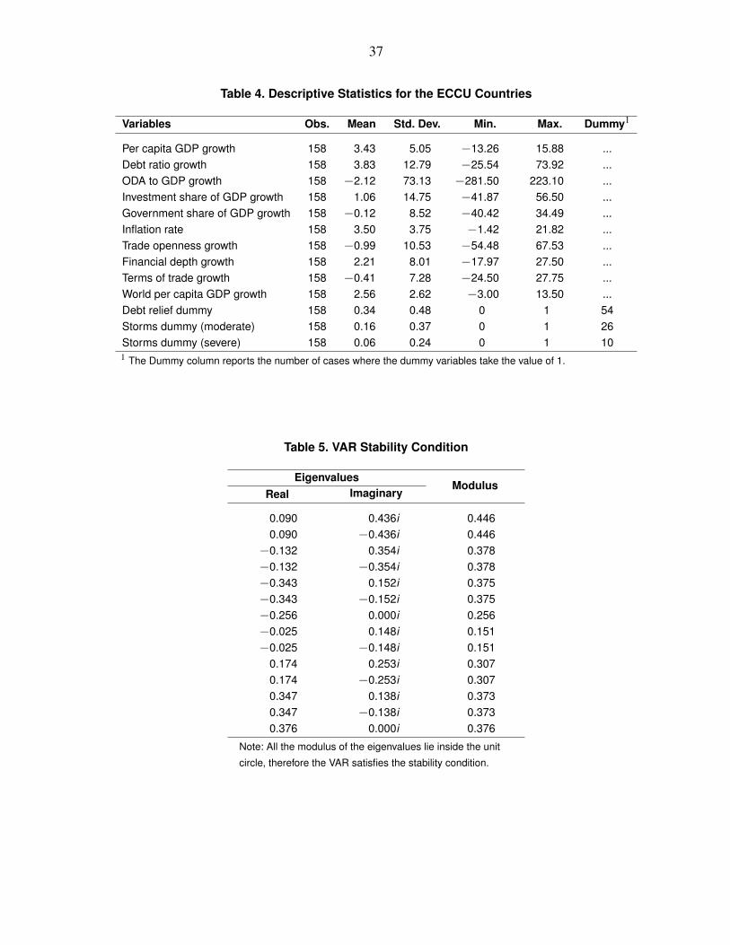
variables which they do not consider.9Table 4 presents summary statistics for the ECCU subsample.

8

of debt forgiveness, debt restructuring and humanitarian aid.10 When a country’s debt is forgivenor a country receives aid in kind (i.e. food, water, blankets, etc.) or cash, these flows immediatlyalleviate pressures to issue new debt to finance the rehabilitation and reconstruction work.Also, restructuring the debt of a country so that its repayment schedule is extended and itsdebt service over the short term is reduced, frees up resources that the government can diverttowards post-disaster needs.

To construct the debt relief dummy I collected data from Paris Club Agreements for the Caribbeancountries included in the sample, as well as data from the World Bank’s Global DevelopmentFinance and the OECD’s OECD.Stat databases.11 The dummy accounts for events in whichCaribbean countries have benefited from a wide array of aid flows covering debt forgiveness,debt restructuring and/or large humanitarian aid flows, but henceforth I will refer to it as the“debt relief” dummy. To make sure that I only capture debt relief events that are economicallymeaningful, I construct the dummy such that it is 1 when the debt relief received surpasses0.01% of GDP.12

The data on natural disasters comes from EM-DAT.13 They collect information on type ofdisaster, number of people killed (fatalities), number of people affected (total affected), and(when available) estimated damages caused by the disaster. I consider two categories of naturaldisasters; storms, and floods and construct the dummy variable for each type of natural disasterby following the measure of intensity proposed by Fomby et al.14 For each type-k natural

10It is important to note that debt forgiveness, debt restructuring, and humanitarian aid are part of ODA flows,that is why the two variables are used in separate specifications.11Given that there are two main sources for the debt relief data, the World Bank and the OECD, I create the debtrelief dummy from both sources adding debt forgiveness, debt restructuring, and humanitarian aid flows. Then, Icombined the two data sets by keeping the data from the source that showed the largest amount in each year foreach recipient country. The Paris Club does not report the amounts of debt relief accorded to countries; hence avalue of 1 was given to the dummy variable whenever there was an agreement with the Paris Club.12I also construct another dummy variable where the debt relief threshold is higher (at least 1% of GDP);however, the results are very similar to the ones for “moderate” debt relief (at least 0.01% of GDP). I choosethe dummy with the lower threshold because it is more relevant in the case of moderate disasters. The results arenot presented in the paper but are available upon request.13For a disaster to be included in EM-DAT at least one of the following criteria must be met: i) at least 10people killed, ii) at least 100 people affected, or iii) a state of emergency was declared or a call for internationalassistance was made. For a detailed explanation of the classification of disaster types see EM-DAT.14Fomby et al. also studied the effects of droughts and earthquakes; however, the small number of these types ofdisasters (one of each) in the usable observations in the sample precluded their analysis in this paper.

9

disaster in country i, in year t, I compute;15

intensityki,t =

1, iff atalitiesk

i,t + 0.3·total affectedki,t

populationi,t> 0.0001

0, otherwise(1)

that is, any natural disaster that affects more than 0.01% of the population of a country isconsidered potentially disruptive enough to have an effect on the economy. The affected populationis a weighted average of the fatalities (with a weight of 1) and the total affected (with a weightof 0.3).16 An alternative to (1) is considered to test the robustness of the results, where theweight of the total affected in the index is 1, instead of the 0.3 in equation (1), that is thefatalities and total affected are given equal weight. Now, to measure the effects of severedisasters a similar index to (1) is constructed where the threshold of the population affectedor killed is increased to 1% of the total population of the country.

Unlike Fomby et al. where they sum all the cases where a type-k natural disaster affects acountry, I simply use the intensity measure as a dummy variable in the estimations. The differenceis that Fomby et al. study the individual effects of an additional disaster in a given year, whereasthis paper studies the effects of having a disastrous year. Fomby et al.’s measure is appropriatefor their analysis. However, in the context of studying the impact on debt which is usuallydecided on an annual basis it is better to analyze the impact of a disastrous year than theimpact of one additional disaster.17 The estimation results using Fomby et al.’s disastersmeasure are similar to those presented in here.18

An alternative measure of the intensity of the disasters can be obtained by using the data onestimated damages as a percent of GDP

intensityki,t =

1, ifdamagesk

i,tGDPi,t

> 0.0001

0, otherwise(2)

This will be used to test the robustness of the results to different measures of the intensity ofthe disasters.

15When more than one type-k natural disaster affects a country in any given year, I aggregate the number offatalities and people affected to construct the intensity index in that year.16The rationale for the weights is that disasters with fatalities are assumed to be more severe than those withoutthem.17For example, when multiple disasters of the same type afflict a country in one year the government is morelikely to respond in a combined manner to the reconstruction needs, rather than to respond on an individualbasis.18The results are not included in the paper but are available upon request.

10

IV. THE ECONOMETRIC MODEL

Following Fomby et al. the econometric model to be used is a fixed effects unbalanced panelvector autoregression with exogenous variables (VARX):

yi,t =α i +Φ1yi,t−1 +Φ2yi,t−2 +Θ0xi,t +Θ1xi,t−1 +Θ2xi,t−2 + ε i,t (3)

where ε i,t is a vector of errors, the countries are indexed by i = 1,2, ...,N, and the time indexfor each country i is t = 1, ...,Ti.

The benchmark model includes seven endogenous variables represented by the yi,t vector, andfour exogenous variables given by the xi,t vector;

yi,t =

Per capita GDP growthi,t

Debt to GDP ratio growthi,t

Investment share of GDP growthi,t

Government share of GDP growthi,t

Inflation ratei,t

Trade openness growthi,t

Financial depth growthi,t

, xi,t =

Stormsi,t

Floodsi,t

Terms of tradei,t

World growthi,t

.

To control for the debt dynamics in the Caribbean, which are influenced by aid flows, debtrelief and debt restructurings I estimate two additional specifications; one where ODA to

GDP growth and another one where a Debt relief dummy are included in xi,t . Below thereis a discussion of why these two variables are treated as exogenous.

A. The Fixed Effects and Bootstrap Bias-corrected Estimators

The fixed effect coefficient for each country is given by α i, which captures the unobserved(time-invariant) heterogeneity of the countries in the Caribbean region. The total number ofusable observations in the panel is denoted by T = ∑

Ni=1 Ti. In equation (3) it is assumed that

the errors are homogeneous, E(ε i,tε′i,t) = Ω for all i and t. The errors are also assumed to be

independent within equations E(ε i,sε′i,t) = 0, for s 6= t, and across equations E(ε i,sε

′j,t) = 0,

for any s and t where i 6= j.

11

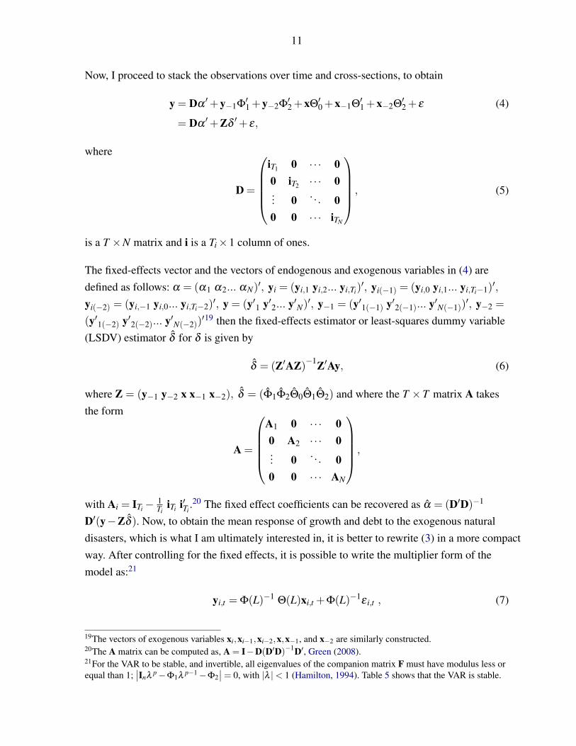
Now, I proceed to stack the observations over time and cross-sections, to obtain

y = Dα′+y−1Φ

′1 +y−2Φ

′2 +xΘ

′0 +x−1Θ

′1 +x−2Θ

′2 + ε (4)

= Dα′+Zδ

′+ ε,

where

D =

iT1 0 · · · 00 iT2 · · · 0... 0 . . . 00 0 · · · iTN

, (5)

is a T ×N matrix and i is a Ti×1 column of ones.

The fixed-effects vector and the vectors of endogenous and exogenous variables in (4) aredefined as follows: α = (α1 α2... αN)

′, yi = (yi,1 yi,2... yi,Ti)′, yi(−1) = (yi,0 yi,1... yi,Ti−1)

′,

yi(−2) = (yi,−1 yi,0... yi,Ti−2)′, y = (y′1 y′2... y′N)′, y−1 = (y′1(−1) y′2(−1)... y′N(−1))

′, y−2 =

(y′1(−2) y′2(−2)... y′N(−2))′19 then the fixed-effects estimator or least-squares dummy variable

(LSDV) estimator δ for δ is given by

δ = (Z′AZ)−1Z′Ay, (6)

where Z = (y−1 y−2 x x−1 x−2), δ = (Φ1Φ2Θ0Θ1Θ2) and where the T ×T matrix A takesthe form

A =

A1 0 · · · 00 A2 · · · 0... 0 . . . 00 0 · · · AN

,

with Ai = ITi− 1Ti

iTi i′Ti.20 The fixed effect coefficients can be recovered as α = (D′D)−1

D′(y−Zδ ). Now, to obtain the mean response of growth and debt to the exogenous naturaldisasters, which is what I am ultimately interested in, it is better to rewrite (3) in a more compactway. After controlling for the fixed effects, it is possible to write the multiplier form of themodel as:21

yi,t = Φ(L)−1Θ(L)xi,t +Φ(L)−1

ε i,t , (7)

19The vectors of exogenous variables xi,xi−1,xi−2,x,x−1, and x−2 are similarly constructed.20The A matrix can be computed as, A = I−D(D′D)−1D′, Green (2008).21For the VAR to be stable, and invertible, all eigenvalues of the companion matrix F must have modulus less orequal than 1;

∣∣Inλ p−Φ1λ p−1−Φ2∣∣= 0, with |λ |< 1 (Hamilton, 1994). Table 5 shows that the VAR is stable.

12

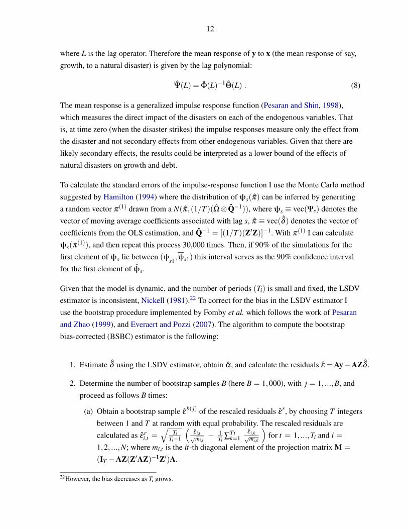
where L is the lag operator. Therefore the mean response of y to x (the mean response of say,growth, to a natural disaster) is given by the lag polynomial:

Ψ(L) = Φ(L)−1Θ(L) . (8)

The mean response is a generalized impulse response function (Pesaran and Shin, 1998),which measures the direct impact of the disasters on each of the endogenous variables. Thatis, at time zero (when the disaster strikes) the impulse responses measure only the effect fromthe disaster and not secondary effects from other endogenous variables. Given that there arelikely secondary effects, the results could be interpreted as a lower bound of the effects ofnatural disasters on growth and debt.

To calculate the standard errors of the impulse-response function I use the Monte Carlo methodsuggested by Hamilton (1994) where the distribution of ψs(π) can be inferred by generatinga random vector π(1) drawn from a N(π,(1/T )(Ω⊗ Q−1)), where ψs ≡ vec(Ψs) denotes thevector of moving average coefficients associated with lag s, π ≡ vec(δ ) denotes the vector ofcoefficients from the OLS estimation, and Q−1 = [(1/T )(Z′Z)]−1. With π(1) I can calculateψs(π

(1)), and then repeat this process 30,000 times. Then, if 90% of the simulations for thefirst element of ψs lie between (ψs1,ψs1) this interval serves as the 90% confidence intervalfor the first element of ψs.

Given that the model is dynamic, and the number of periods (Ti) is small and fixed, the LSDVestimator is inconsistent, Nickell (1981).22 To correct for the bias in the LSDV estimator Iuse the bootstrap procedure implemented by Fomby et al. which follows the work of Pesaranand Zhao (1999), and Everaert and Pozzi (2007). The algorithm to compute the bootstrapbias-corrected (BSBC) estimator is the following:

1. Estimate δ using the LSDV estimator, obtain α , and calculate the residuals ε =Ay−AZδ .

2. Determine the number of bootstrap samples B (here B = 1,000), with j = 1, ...,B, andproceed as follows B times:

(a) Obtain a bootstrap sample εb( j) of the rescaled residuals ε

r, by choosing T integersbetween 1 and T at random with equal probability. The rescaled residuals arecalculated as εr

i,t =√

TiTi−1

(ε i,t√mi,t− 1

Ti∑

Tik=1

ε i,k√mi,k

)for t = 1, ...,Ti and i =

1,2, ...,N; where mi,t is the it-th diagonal element of the projection matrix M =

(IT −AZ(Z′AZ)−1Z′)A.

22However, the bias decreases as Ti grows.

13

(b) Calculate a bootstrap sample yb( j)=Dα′+Zb( j)δ

′+ ε

b( j), where Zb( j)=(yb( j)−1 yb( j)

−2 xx−1 x−2), yb( j)

i,−1 = yi,−1 and with initialization yb( j)i,0 = yi,0 for i = 1, ...,N.

(c) Obtain the LSDV estimator δb( j)

= (Zb( j)′AZb( j))−1Zb( j)′Ayb( j), and the mean

responses Ψb( j)

(L) =[Φ

b( j)(L)]−1

Θb( j)

(L).

3. Then calculate the bootstrap bias-corrected (BSBC) mean response Ψs for the s-lag as

Ψs = 2Ψs−1B

B

∑j=1

Ψb( j)s , for s = 1,2, ...

where Ψs is the LSDV mean response of Ψs.

To calculate the standard errors of the BSBC impulse-responses I follow a procedure similarto the Monte Carlo method used for the LSDV estimator described above. First, I generateB bootstrapped samples for each of the δ

b( j)in the above procedure and calculate the BSBC

mean response Ψ( j) for each of the samples using the BSBC algorithm to obtain ψ(1)

, ...,ψ(B).

And again, if 90% of the simulations for the first element of ψs lie between (ψs1,ψs1) thisinterval serves as the 90% confidence interval for the first element of ψs.23

B. Diagnostic Tests

Before proceeding with the estimations and presenting the results it is important to test forthe stationarity of the time series involved, and choose the lag structure of the model. Forthe former, I perform panel and individual series unit-root tests, and for the latter I use thelikelihood ratio test and the Akaike (AIC) and Schwarz (SBIC) information criteria to selectthe lag length. Additionally, I do Granger causality tests to determine if ODA to GDP growth

and the Debt relief dummy should be included in the model as endogenous or exogenousvariables.

First, I employ the Im, Pesaran, Shin (IPS) panel unit-root tests for each of the series, becausethe IPS test is appropriate for unbalanced panels such as the one in this paper. The resultspresented in column 1 of Table 6 indicate that the null hypothesis that all the panels havea unit-root is rejected in all the cases. Similarly, the individual unit root-tests, AugmentedDickey-Fuller (ADF) and Phillips-Perron (PP), show that the majority of countries do notexhibit signs of unit-roots in the series. Columns 2 and 3 of Table 6 present the percentage of

23The model is estimated in Matlab building on the code developed by Fomby et al.

14

countries that reject the presence of a unit-root for each variable.24 The evidence suggests thatthe variables, in log differences, are appropriate to be used in a VARX model.

The lag structure of the VARX is chosen by using the AIC and SBIC information criteria andperforming likelihood ratio tests. Table 7 shows the information criteria and likelihood ratiostatistics for the benchmark model testing up to three lags for the endogenous and exogenousvariables, represented by p and q, respectively.25 The information criteria point towards amodel with p = q = 1, while the likelihood ratio tests suggests that the model should includethree lags (p = q = 3). As a compromise between the two approaches I choose 2 lags for allthe estimations. The likelihood ratio tests suggests that the dynamics are not well captured bya one-lag VARX, while the information criteria suggest that the information loss with 3 lagsis higher, hence, 2 lags are used to strike a balance between the two objectives.26

Finally, I test the endogeneity/exogeneity of the ODA to GDP growth and the Debt relief

dummy variables by doing Granger causality tests. The tests statistics in Table 8 show thatboth variables are not Granger caused by the endogenous variables in the model, that is, theycan be treated as exogenous.27 Therefore, in all the simulations both variables are treated asexogenous and are included in the xi,t vector.

The exogeneity result for debt relief was expected, as there is an argument to be made aboutits treatment as an exogenous shock. For example the debt initiative for Heavily IndebtedPoor Countries (HIPC) launched by the World Bank and the IMF in 1996 relaxed its eligibilityrequirements in 1999. Hence, countries that benefited after 1999 might have not benefitedbefore. Furthermore, anecdotal evidence suggests that donors are more willing to provideaid for some types of disasters than others. For example, in the case of St. Vincent and theGrenadines that was hit by hurricane Tomas in October 2010, and by floods in April 2011,

24World per capita GDP growth cannot be tested as a panel because it is a variable that is shared by allcountries, so the results presented in Table 6 are the corresponding p-values for the ADF and PP tests.25I use the modified likelihood ratio test suggested by Sims (1980) to take into account the small sample bias,under the null hypothesis that the set of variables was generated from a Gaussian VARX with p0 = q0 lagsagainst the alternative specification of p1 = q1 = p0 + 1 lags. This likelihood ratio test has an asymptoticalχ2 distribution with degrees of freedom equal to the number of restrictions imposed under H0, which in this caseis equal to K2(p1− p0)+KD(q1− q0), where K and D are the number of endogenous and exogenous variablesin the model, respectively.26As an added bonus, choosing two lags makes the comparison with the results of Fomby et al. straightforward,since they also use the same lag structure.27I use a likelihood ratio test with an asymptotic χ2 distribution with degrees of freedom equal to the numberof restrictions (n1n2 p), under the null hypothesis that the n1 variables represented by y1 are exogenous withrespect to the n2 variables represented by y2. In this case y1 is either ODA or debt relief (the variables weretested separately, because they will be used like that in the estimations), and y2 are all the endogenous variablesin the model, p = 2 as discussed above.

15

both with similar estimated damages, the donor response was considerably higher for thehurricane than for the floods (IMF, 2011a,b).28 Also, Eisensee and Strömberg (2007) findthat relief decisions are driven by news coverage of disasters, with disasters that get morecoverage receiving more aid.29

However, the result showing that ODA is exogenous to the economic conditions (growth,inflation, government spending, investment, debt, etc.) of the recipient countries was surprising.ODA includes a wide array of flows, which not only encompass humanitarian aid after adisaster, or debt relief, but also development projects that one would expect to be partiallydependent on the macroeconomic circumstances of the recipient country.

V. RESULTS

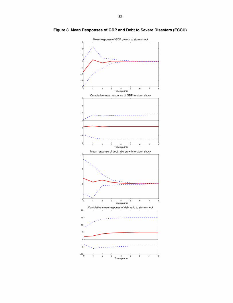
This section presents and discusses the results of the effects of natural disasters (i.e. stormsand floods) on economic growth and debt. The focus is on the dynamic effects and the adjustmentpath after a natural disaster. These effects are studied by using the mean impulse responsefunctions and the mean cumulative response of GDP growth and the debt ratio growth toeach type of disaster. The results are shown in Figures 1 to 10, where I present the mean andcumulative mean responses for years 0 through 8 (where 0 denotes the year of the disaster)and their corresponding confidence intervals depicting the 10% tails of the distribution.30 Thecharts in the figures are organized as follows: the first column shows the effects of storms,while the second column contains the effects of floods; the upper half of the figures depictsthe effects on GDP, and the bottom half the effect on the debt ratio. The results presented inthis section correspond to the BSBC estimator.

28The estimated damages of hurricane Tomas were US$31 million while the ones for the floods were US$26million. However, the grants and humanitarian aid received for the hurricane were almost three times larger thanthe ones received for the floods.29A Granger causality test of the debt relief dummy to the exogenous disaster shocks shows that debt relief isnot Granger caused by the natural disasters dummies. That is, natural disasters are not a good predictor of debtrelief assistance received by affected countries (Table 9). Similarly, Granger causality tests of the debt reliefdummy to each type of disaster individually (floods, and storms) show that neither disaster by itself is a goodpredictor of debt relief (the results are available upon request).30The confidence intervals are constructed using the procedure explained in the previous section.

16

A. The benchmark model

In the immediate aftermath of natural disasters there are several outcomes that can decelerategrowth. Part of the capital stock (including basic infrastructure such as roads, bridges, schools,housing, etc.) is damaged or destroyed, slowing or even halting production activity. Delivery,transportation, and communication systems are disrupted affecting supply chains. And resourcesthat could have been used in the production process need to be devoted to clean-up, rehabilitation,and reconstruction activities.

The results for the benchmark model show that both storms and floods have an immediatenegative effect on output growth, albeit none appear to be statistically significant. The benchmarkmodel’s results are presented in Figure 1 for moderate disasters and in Figure 2 for severedisasters. The effects of storms appear to be larger than those for floods in the case of moderatedisasters; on impact GDP growth falls by more than half a percentage point in the case ofmoderate storms, and it falls by 0.1 percentage points in the case of moderate floods. Asexpected, the effects of severe disasters on output growth are larger than those of moderateones; in particular the immediate effect that severe disasters bring is close to 3 percentagepoints in the case of floods and above 1 percentage point in the case of storms.

The recovery path after a disaster hits shows that the economy enjoys a small rebound ineconomic activity in year 1 after storms and year 2 after floods (year 3 after severe floods).However, this is a short lived effect. This suggests that after a natural disaster there is a concentratedeffort at reconstruction and rehabilitation that lasts about a year after which a relapse to negativegrowth follows. After the fifth or sixth year the effects of the disasters are small and tend todisappear. The rebound in economic activity in the years after a natural disaster is associatedwith higher construction activity to replace or repair basic infrastructure and housing, increasedagricultural activity to rehabilitate and replant crops, and a possible productivity boost fromreplacing low quality capital with high quality one.

In the case of moderate storms the recovery phase is so small that the economy never recoversentirely from the shock and the economy finds itself about 0.5 percent below the level it wouldhave had in the absence of the disaster. But after a moderate flood the economic recovery islarge enough to have a slightly positive cumulative effect on the level of output. However, itis important to note that for both storms and floods the cumulative effects are not statisticallysignificant. Interestingly, the cumulative effects after severe disasters are reversed. That is,after a severe storm the economic recovery in the first few years is sufficient to have the economyslightly above its non-disaster output level. However, in the case of severe floods there seems

17

to be only a small rebound in GDP growth linked to a recovery phase and hence the cumulativeeffect on output is negative.

Different types of government expenditure, and their impact on growth, could explain whymoderate storms have a negative cumulative effect on GDP while severe storms have a positiveeffect. Smaller storms usually have a limited impact on infrastructure, but have large effectson the livelihood of people. In this case the government is expected to increase social assistanceprograms to help people get back on their feet, but the effect on growth is likely to be small.Severe storms on the other hand have larger effects on infrastructure requiring big investmentsfor reconstruction, which in turn help the economic recovery. The length of the recoveryphase also supports this view. Moderate storms have a short recovery of just one year, butsevere storms show a longer recovery phase of almost 5 years; after all large reconstructionprojects take years to complete.

In the case of floods the results show the opposite cumulative effects; moderate floods have apositive impact on growth and severe floods a negative one. This is consistent with Fomby et

al.’s finding that moderate floods have a lasting positive effect on growth, while severe oneshave a negative effect. They argue that moderate floods have a beneficial effect on growththrough higher land productivity. However, I find that moderate floods have an initial negativeeffect, although not statistically significant, which could be the case given that Caribbeancountries have small agricultural sectors and therefore would tend to benefit less from moderatefloods.

Before moving to the effects on debt, I replicate in my Caribbean sample the exact modelused by Fomby et al. by excluding all the debt related variables from the model. The resultsare presented in Figures A1 and A2 in the Appendix. The results show that excluding debtfrom the VARX overestimates the negative effect of natural disasters on GDP. When debt isabsent from the estimations (Figures A1 and A2) the initial drop in GDP is larger for bothtypes of disasters, and for both moderate and severe intensities. What is more, when debt isexcluded, in the case of moderate storms the initial fall in GDP growth is statistically significant(borderline), and there is no recovery phase in the years following the disaster. The recoveryphase is also more subdued in the case of severe storms and floods. Excluding debt biases theestimates of the disasters on growth, which capture part of the negative effect of debt on GDPhence showing a larger drop in economic activity after a disaster strikes. The negative effectof debt on growth after a disaster is caused partly by the high opportunity cost of increasingdebt to replace damaged capital instead of investing in new capital.

18

These results clearly point to the need of including public debt as part of the endogenousvariables in the model. Both the initial decline in economic activity and the reconstructionthat takes place in the aftermath of the disasters have a repercussion in public finances (revenueand expenditure), and create financing needs that increase public debt in the absense of fiscalbuffers. Including this variable in the model is crucial to understand the dynamic effects ofnatural disasters on the economy.

Turning the analysis to debt (bottom half of Figures 1 and 2), the results show that both moderateand severe floods increase the debt ratio growth rate.31 In the case of severe floods the effectis a significant increase in the growth of the debt ratio of about 16 percentage points. However,the large increase in debt to finance rehabilitation and reconstruction activities after severefloods is not reflected in a pickup of economic activity until the third year of the recoveryphase. Given the large opportunity costs involved in increasing debt and mobilizing resourcesto replace the damaged capital stock instead of investing in new capital, it is not entirelysurprising that the increase in government debt is not reflected in a stronger recovery.

Surprisingly, the effect that severe storms have on debt is negative and significant, namely, thedebt ratio seems to decline after a storm hits a Caribbean country. The decline in the growthrate of the debt ratio lasts for two periods after a moderate storm, and for three periods aftera severe storm. In the latter case the initial decline in the growth rate of the debt to GDP ratiois significant and close to 8 percentage points. An explanation of the decline in the debt ratiogrowth rate after severe storms is explored in the next subsection.

B. The role of debt relief and ODA

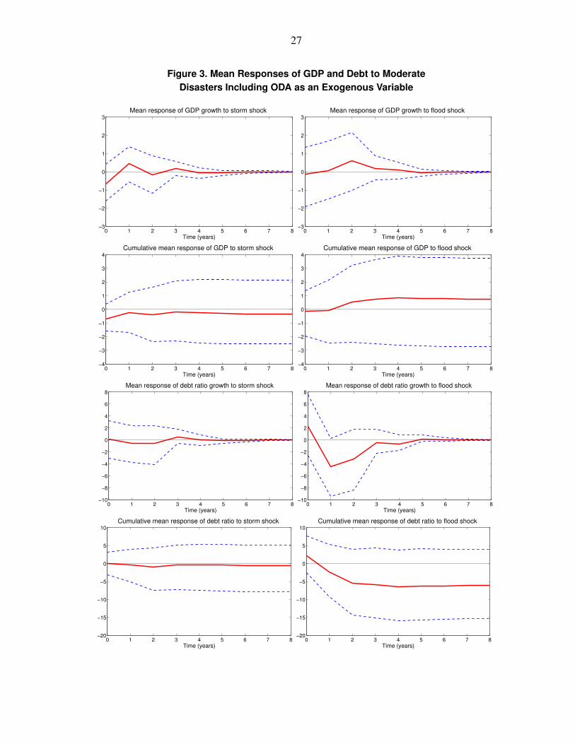
In order to understand the dynamics behind the debt results, I explore the effects that debtforgiveness, debt restructuring, humanitarian aid, and in general ODA play in the aftermathof natural disasters in the Caribbean. To do that, I use two alternative specifications of themodel, one with ODA and another one with debt relief as part of the exogenous variables.32

The results for ODA are presented in Figures 3 and 4, while Figures 5 and 6 cover the casewith the debt relief dummy.

31The increase in the debt ratio is not only a consequence of lower growth but also of an actual increase in thedebt level to finance the recovery and reconstruction activity. The estimations use the debt to GDP ratio becauseit is a more informative measure of indebtedness than debt levels by themselves. However, estimations for thegrowth rate of debt levels show very similar results to the ones in Figures 1 through 10 (available upon request).32The debt relief dummy comprises debt forgiveness, debt restructuring and humanitarian aid flows that arelarger than 0.01% of the recipient’s country GDP.

19

1. The model with ODA

Here, I study the possibility that the growth of ODA as a percent of GDP has an influence ondebt after a natural disaster. Figure 3 presents the results for moderate disasters and Figure 4the results for severe disasters. Although, a priori this alternative seems an interesting avenueof exploration, the results do not show any material difference compared to the benchmarkmodel (Figures 1 and 2). These results are consistent with the findings of Raddatz (2009)where ODA only has a modest and not significant reduction of the effects of natural disasters.The results are not surprising considering that ODA includes a wide array of flows, which notonly encompass humanitarian aid after a disaster, or debt relief, but also long term projectswhich are not influenced by short term considerations, such as natural disasters.

2. The model with debt relief

Now, we study the model including the debt relief dummy. This is probably a more relevantmeasure of the development assistance flows that are more closely related to natural disastersand/or debt issues, and might shed light to the role that debt relief plays in the aftermath ofnatural disasters. However, there is a caveat; the results, although different from what waspresented in Figures 1 and 2, are not statistically significant. Therefore, all the results withexogenous debt relief are treated as weak evidence of the effects of debt relief in the aftermathof natural disasters (Figures 5 and 6).

The results for growth are very similar to those when debt relief was not included. However,on the debt front, after controlling for debt relief flows we see that on the first 3 years after amoderate storm hits a country there is an initial increase in debt, although still not significant.When including the debt relief dummy the cumulative effect shows an increase in the debtratio level of about 3 percent, which contrasts with the case without the dummy where theeffect on the debt ratio was negligible.33 This suggests that debt relief helps countries financethe reconstruction activity after a disaster by ameliorating, with external aid funds, the demandto increase public debt. But the evidence is not conclusive, which might be the case if theimpact of debt relief is small.

After a severe storm, even after controlling for debt relief, the mean response of the debtratio growth still shows a significant decline. However, the decline is smaller (7.6 percentage

33The exclusion of the debt dummy biases the estimates of the disasters on the debt to GDP ratio that capturepart of the negative effect of debt relief on debt; that is, the fact that debt relief is expected to reduce debt.

20

points) when controlling for debt relief than when not (7.9 percentage points). This indicatesthat there still are some effects that exert influence over debt that are not captured by themodel. The debt results after flood shocks remain unaltered when incorporating the debt reliefdummy in the model. The initial mean response, to a severe flood, of the debt to GDP ratiogrowth is still an increase close to 15 percentage points.

So far, we have seen that different types of natural disasters have a negative effect on output,but they have different effects on debt. While severe floods increase debt, severe storms seemto reduce it, even after controlling for the effects of debt relief. But, as will be shown nextthere is a subsample of countries in the Caribbean where the effects of storms on debt arequite different.

C. Storms in the Eastern Caribbean Currency Union

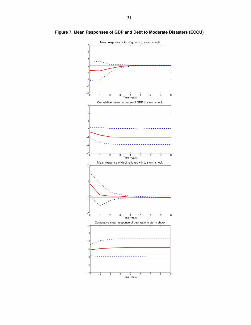
This subsection studies the effects of storms in the 6 countries of the ECCU. I only estimatethe model with storms because the small number of floods in the sample for the sub-region(only three moderate floods but zero severe ones) precludes their analysis in the model. Themodel for the ECCU is estimated with just one lag of the endogenous and exogenous variables(p = q = 1) because with the smaller sample size it is not possible to estimate the model withtwo lags as was done for the broader Caribbean. The results for moderate and severe stormsin the ECCU are presented in Figures 7 to 10.34

In the ECCU, the immediate effect of a moderate storm (Figure 7) is a decline in GDP growthof about 0.7 percentage points (but not statistically significant), in line with the results forthe broader Caribbean. However, unlike the rest of the Caribbean the ECCU countries do notseem to enjoy a strong recovery after moderate storms, instead seeing their economies declinefurther in the following year. The cumulative impact is a borderline significant lower level ofGDP (about 2 percent lower) two years after a storm.

The effect on debt, in this case, is clearly positive and significant. During the year that theECCU countries are hit by a storm the debt to GDP ratio grows faster by almost 5 percentagepoints, with a cumulative effect that shows a debt to GDP level that is more than 5 percenthigher after 8 years.35 A possible explanation to why storms significantly increase debt in

34 The results with ODA as an exogenous variable are not presented because, as shown above, they also havelittle effect on the results for the ECCU. However, they are available upon request.35 Noy and Nualsri (2011) find that a year and a half after a disaster the debt to GDP ratio is higher by morethan 8 percent of GDP. However, their results might be upwardly biased since they do not control for otherdeterminants of output and debt in their estimations.

21

the ECCU but not so in the broader Caribbean could be related to the fact that the ECCUcountries are smaller (in population and land size) and more vulnerable to natural disasters(see Table 7.4 in Rasmussen, 2006) than other Caribbean countries. The smaller size not onlyresults in a larger portion of the country being affected when a disaster strikes, but could alsosuggest limited capacity to respond to the crisis without requiring an increase in debt.

Higher debt and lower growth without a strong recovery phase suggests that the increase indebt is not supporting the economic recovery. These results are consistent with the idea that inthe case of moderate storms the government is borrowing to support the affected populationwith social assistance programs that have little impact on growth.

The results in Figure 8 show that the immediate effect of a severe storm is a decline in growthof close to 2 percentage points, but not significant (borderline), with a negative cumulativeeffect in the long run due to a very small recovery in the year after the storm strikes. Although,severe storms in the ECCU increase the debt ratio growth by almost 2 percentage points onimpact, with a cumulative increase in debt of 5 percent by year 8, the results are not statisticallysignificant. The difference in results with the broader Caribbean where severe storms have apositive cumulative effect on output could be related to the response of debt. While in thebroader Caribbean debt declines, in the ECCU debt increases, reconstruction activity is lower,and the cumulative effect on GDP of severe storms is negative.

1. The role of debt relief

The positive effects of debt relief after a natural disaster are similar in the case of the ECCU(Figures 9 and 10). The effects on growth for both moderate and severe storms appear to besmall. However, after controlling for the effect of debt relief the impact on debt is larger bothin the year of the event and over the long run for moderate and severe storms. Again, we cansee that there is weak evidence that debt relief helps financing the costs associated with anatural disaster, and reducing the impact on debt. Hence, debt relief seems to play a role ineasing the negative consequences of natural disasters in the Caribbean, and in helping thecountries in the reconstruction phase.

D. Robustness

All the results presented so far were obtained from the BSBC estimator. Additionally, all theresults contained in the paper were also estimated using the LSDV estimator as a robustness

22

check. The LSDV results turned out to be very similar to the BSBC ones, suggesting thatgiven the average time sample of 31 years in the data, the LSDV estimator is a good approximation,that is, the LSDV estimator bias is small. Since the results are very similar they are not includedin the paper but are available upon request.

The figures in the Appendix, present robustness checks of the results for the benchmark modeland the alternative specification including the debt relief dummy. Figures A3 and A4 usetotal affected as an alternative measure of disaster intensity.36 Figures A5 and A6 present theresults when the estimated damages in U.S. dollars are used to construct the disaster intensitydummy variable. The robustness estimations show that the qualitative response to a disaster atyear 0 is robust to the different measures of disaster intensity. However, the cumulative effectsseem to depend on the measure used.

VI. CONCLUSIONS

This paper studied the effects of natural disasters in the Caribbean economies by using apanel VAR with exogenous variables. Three models have been estimated; a benchmark modelthat analyzes the effect of moderate and severe storms and floods on debt and growth, andtwo alternative models that look at the effects that debt relief and ODA play in the aftermathof natural disasters.

In general, the results show that both storms and floods have a negative effect on growth, withsevere disasters generating larger drops in output. I find that including debt in the model isimportant because its exclusion overestimates the impact of disasters on output. When debtis excluded the coefficients for disasters capture part of the negative effect of debt on growthbiasing the estimates, and showing a larger drop in economic activity after a disaster strikes.The increase in the debt ratio after a disaster is not only the result of lower GDP, but also anincrease in debt levels to finance the recovery and reconstruction activity.

The results indicate that floods increase debt while storms (in particular severe ones) do not.This is partially explained by the role that external debt relief and aid flows play in the recoveryafter the disasters; where storms seem to benefit from aid flows while floods do not. However,the evidence is weak and far from conclusive. The small effect of debt relief in the responseof debt to floods could suggest that floods do not attract as much attention and hence aid asstorm do. After all, storms in the Caribbean are usually hurricanes that get global coverage

36 This is the case where both fatalities and total affected have a weight of 1 in the intensity measure.

23

and invite more attention and as Eisensee and Strömberg (2007) show that affects the reliefdecision of donors. However, neither floods nor storms (separately or combined) are goodpredictors of a country receiving debt relief, therefore this results should be interpreted carefully.

In the case of the ECCU, the results give a different picture of the effects of storms on debt.Moderate and severe storms increase debt in the short run as in the long run, however, onlythe effect of moderate storms is statistically significant. The effect of storms on growth isnegative; with severe storms initially having a larger negative effect.

Higher debt does not seem to support stronger economic activity during the recovery phase ineither moderate or severe disasters. In the case of moderate disasters this might be explainedby the type of expenditures that governments incur. I suggest the possibility that moderatedisasters likely require more expenditure on social assistance for the affected populationwhile severe ones need a larger component of investment in infrastructure, which is moresupportive of an economic rebound in activity. However, even in the case of infrastructureinvestment, the opportunity cost involved in replacing damaged capital goods instead of investingin new capital results in a weaker recovery than expected a priori, especially when it involvesincreasing debt. More research is needed to fully understand these connections.

The two alternative model specifications considering the effects of aid flows show that generalaid flows (ODA) do not have much of an effect in the aftermath of natural disasters. On theother hand, what could be called “targeted aid flows”37 after a storm, seem to have a rolein lessening the negative effects on debt. Particularly, there is weak evidence that debt reliefhelps to reduce the pressure on debt accumulation to finance the reconstruction activity afterstorms.

The evidence suggests that debt relief flows are exogenously determined, that is, they do notrespond to the economic conditions of the receiving country, and the relief response seems tobe uneven among disasters. If that is the case, it suggests that aid recipient countries cannotalways count on the good will of their donors. And, this has economic policy implicationsfor Caribbean countries. Disaster prone countries should expect debt to rise in the aftermathof disasters (especially if they don’t receive foreign aid), and consequently should attemptto keep sustainable debt levels, and create enough fiscal space to be able to finance their ownrecovery. Other measures such as establishing disaster funds and increasing insurance coveragefor the public and private sector, should also be pursued.38 Additionally, countries should

37These are: debt relief, debt restructuring, and humanitarian aid that are captured in the debt relief dummy.38For an in depth analysis of the different options available to governments in the aftermath of disasters seeCashin and Dyczewski (2006).

24

seek to build resilience by integrating climate and disaster risk into their policy frameworksboth at the macro and micro levels.39

39For a comprehensive analysis of how to build resilience to disasters see World Bank (2013), and for a detaileddescription of macro policy options in response to and preparation for disasters see Laframboise and Loko(2012).

25

Figure 1. Mean Responses of GDP and Debt to Moderate Disasters

0 1 2 3 4 5 6 7 8−3

−2

−1

0

1

2

3

Time (years)

Mean response of GDP growth to storm shock

0 1 2 3 4 5 6 7 8−3

−2

−1

0

1

2

3

Time (years)

Mean response of GDP growth to flood shock

0 1 2 3 4 5 6 7 8−4

−3

−2

−1

0

1

2

3

4

Time (years)

Cumulative mean response of GDP to storm shock

0 1 2 3 4 5 6 7 8−4

−3

−2

−1

0

1

2

3

4

Time (years)

Cumulative mean response of GDP to flood shock

0 1 2 3 4 5 6 7 8−10

−8

−6

−4

−2

0

2

4

6

8

Time (years)

Mean response of debt ratio growth to storm shock

0 1 2 3 4 5 6 7 8−10

−8

−6

−4

−2

0

2

4

6

8

Time (years)

Mean response of debt ratio growth to flood shock

0 1 2 3 4 5 6 7 8−20

−15

−10

−5

0

5

10

Time (years)

Cumulative mean response of debt ratio to storm shock

0 1 2 3 4 5 6 7 8−20

−15

−10

−5

0

5

10

Time (years)

Cumulative mean response of debt ratio to flood shock

26

Figure 2. Mean Responses of GDP and Debt to Severe Disasters

0 1 2 3 4 5 6 7 8−8

−6

−4

−2

0

2

4

Time (years)

Mean response of GDP growth to storm shock

0 1 2 3 4 5 6 7 8−8

−6

−4

−2

0

2

4

Time (years)

Mean response of GDP growth to flood shock

0 1 2 3 4 5 6 7 8−15

−10

−5

0

5

10

Time (years)

Cumulative mean response of GDP to storm shock

0 1 2 3 4 5 6 7 8−15

−10

−5

0

5

10

Time (years)

Cumulative mean response of GDP to flood shock

0 1 2 3 4 5 6 7 8−30

−20

−10

0

10

20

30

Time (years)

Mean response of debt ratio growth to storm shock

0 1 2 3 4 5 6 7 8−30

−20

−10

0

10

20

30

Time (years)

Mean response of debt ratio growth to flood shock

0 1 2 3 4 5 6 7 8−30

−20

−10

0

10

20

30

40

50

Time (years)

Cumulative mean response of debt ratio to storm shock

0 1 2 3 4 5 6 7 8−30

−20

−10

0

10

20

30

40

50

Time (years)

Cumulative mean response of debt ratio to flood shock

27

Figure 3. Mean Responses of GDP and Debt to ModerateDisasters Including ODA as an Exogenous Variable

0 1 2 3 4 5 6 7 8−3

−2

−1

0

1

2

3

Time (years)

Mean response of GDP growth to storm shock

0 1 2 3 4 5 6 7 8−3

−2

−1

0

1

2

3

Time (years)

Mean response of GDP growth to flood shock

0 1 2 3 4 5 6 7 8−4

−3

−2

−1

0

1

2

3

4

Time (years)

Cumulative mean response of GDP to storm shock

0 1 2 3 4 5 6 7 8−4

−3

−2

−1

0

1

2

3

4

Time (years)

Cumulative mean response of GDP to flood shock

0 1 2 3 4 5 6 7 8−10

−8

−6

−4

−2

0

2

4

6

8

Time (years)

Mean response of debt ratio growth to storm shock

0 1 2 3 4 5 6 7 8−10

−8

−6

−4

−2

0

2

4

6

8

Time (years)

Mean response of debt ratio growth to flood shock

0 1 2 3 4 5 6 7 8−20

−15

−10

−5

0

5

10

Time (years)

Cumulative mean response of debt ratio to storm shock

0 1 2 3 4 5 6 7 8−20

−15

−10

−5

0

5

10

Time (years)

Cumulative mean response of debt ratio to flood shock

28

Figure 4. Mean Responses of GDP and Debt to SevereDisasters Including ODA as an Exogenous Variable

0 1 2 3 4 5 6 7 8−8

−6

−4

−2

0

2

4

Time (years)

Mean response of GDP growth to storm shock

0 1 2 3 4 5 6 7 8−8

−6

−4

−2

0

2

4

Time (years)

Mean response of GDP growth to flood shock

0 1 2 3 4 5 6 7 8−15

−10

−5

0

5

10

Time (years)

Cumulative mean response of GDP to storm shock

0 1 2 3 4 5 6 7 8−15

−10

−5

0

5

10

Time (years)

Cumulative mean response of GDP to flood shock

0 1 2 3 4 5 6 7 8−30

−20

−10

0

10

20

30

Time (years)

Mean response of debt ratio growth to storm shock

0 1 2 3 4 5 6 7 8−30

−20

−10

0

10

20

30

Time (years)

Mean response of debt ratio growth to flood shock

0 1 2 3 4 5 6 7 8−30

−20

−10

0

10

20

30

40

50

Time (years)

Cumulative mean response of debt ratio to storm shock

0 1 2 3 4 5 6 7 8−30

−20

−10

0

10

20

30

40

50

Time (years)

Cumulative mean response of debt ratio to flood shock

29

Figure 5. Mean Responses of GDP and Debt to Moderate DisastersIncluding the Debt Relief Dummy as an Exogenous Variable

0 1 2 3 4 5 6 7 8−3

−2

−1

0

1

2

3

Time (years)

Mean response of GDP growth to storm shock

0 1 2 3 4 5 6 7 8−3

−2

−1

0

1

2

3

Time (years)

Mean response of GDP growth to flood shock

0 1 2 3 4 5 6 7 8−4

−3

−2

−1

0

1

2

3

4

Time (years)

Cumulative mean response of GDP to storm shock

0 1 2 3 4 5 6 7 8−4

−3

−2

−1

0

1

2

3

4

Time (years)

Cumulative mean response of GDP to flood shock

0 1 2 3 4 5 6 7 8−10

−8

−6

−4

−2

0

2

4

6

8

Time (years)

Mean response of debt ratio growth to storm shock

0 1 2 3 4 5 6 7 8−10

−8

−6

−4

−2

0

2

4

6

8

Time (years)

Mean response of debt ratio growth to flood shock

0 1 2 3 4 5 6 7 8−20

−15

−10

−5

0

5

10

Time (years)

Cumulative mean response of debt ratio to storm shock

0 1 2 3 4 5 6 7 8−20

−15

−10

−5

0

5

10

Time (years)

Cumulative mean response of debt ratio to flood shock

30

Figure 6. Mean Responses of GDP and Debt to Severe DisastersIncluding the Debt Relief Dummy as an Exogenous Variable

0 1 2 3 4 5 6 7 8−8

−6

−4

−2

0

2

4

Time (years)

Mean response of GDP growth to storm shock

0 1 2 3 4 5 6 7 8−8

−6

−4

−2

0

2

4

Time (years)

Mean response of GDP growth to flood shock

0 1 2 3 4 5 6 7 8−15

−10

−5

0

5

10

Time (years)

Cumulative mean response of GDP to storm shock

0 1 2 3 4 5 6 7 8−15

−10

−5

0

5

10

Time (years)

Cumulative mean response of GDP to flood shock

0 1 2 3 4 5 6 7 8−30

−20

−10

0

10

20

30

Time (years)

Mean response of debt ratio growth to storm shock

0 1 2 3 4 5 6 7 8−30

−20

−10

0

10

20

30

Time (years)

Mean response of debt ratio growth to flood shock

0 1 2 3 4 5 6 7 8−30

−20

−10

0

10

20

30

40

50

Time (years)

Cumulative mean response of debt ratio to storm shock

0 1 2 3 4 5 6 7 8−30

−20

−10

0

10

20

30

40

50

Time (years)

Cumulative mean response of debt ratio to flood shock

31

Figure 7. Mean Responses of GDP and Debt to Moderate Disasters (ECCU)

0 1 2 3 4 5 6 7 8−4

−3

−2

−1

0

1

2

3

Time (years)

Mean response of GDP growth to storm shock

0 1 2 3 4 5 6 7 8−6

−4

−2

0

2

4

6

Time (years)

Cumulative mean response of GDP to storm shock

0 1 2 3 4 5 6 7 8−5

0

5

10

Time (years)

Mean response of debt ratio growth to storm shock

0 1 2 3 4 5 6 7 8−10

−5

0

5

10

15

20

Time (years)

Cumulative mean response of debt ratio to storm shock

32

Figure 8. Mean Responses of GDP and Debt to Severe Disasters (ECCU)

0 1 2 3 4 5 6 7 8−4

−3

−2

−1

0

1

2

3

Time (years)

Mean response of GDP growth to storm shock

0 1 2 3 4 5 6 7 8−6

−4

−2

0

2

4

6

Time (years)

Cumulative mean response of GDP to storm shock

0 1 2 3 4 5 6 7 8−5

0

5

10

Time (years)

Mean response of debt ratio growth to storm shock

0 1 2 3 4 5 6 7 8−10

−5

0

5

10

15

20

Time (years)

Cumulative mean response of debt ratio to storm shock

33

Figure 9. Mean Responses of GDP and Debt to Moderate DisastersIncluding the Debt Relief Dummy as an Exogenous Variable (ECCU)

0 1 2 3 4 5 6 7 8−4

−3

−2

−1

0

1

2

3

Time (years)

Mean response of GDP growth to storm shock

0 1 2 3 4 5 6 7 8−6

−4

−2

0

2

4

6

Time (years)

Cumulative mean response of GDP to storm shock

0 1 2 3 4 5 6 7 8−5

0

5

10

Time (years)

Mean response of debt ratio growth to storm shock

0 1 2 3 4 5 6 7 8−10

−5

0

5

10

15

20

Time (years)

Cumulative mean response of debt ratio to storm shock

34

Figure 10. Mean Responses of GDP and Debt to Severe DisastersIncluding the Debt Relief Dummy as an Exogenous Variable (ECCU)

0 1 2 3 4 5 6 7 8−4

−3

−2

−1

0

1

2

3

Time (years)

Mean response of GDP growth to storm shock

0 1 2 3 4 5 6 7 8−6

−4

−2

0

2

4

6

Time (years)

Cumulative mean response of GDP to storm shock

0 1 2 3 4 5 6 7 8−5

0

5

10

Time (years)

Mean response of debt ratio growth to storm shock

0 1 2 3 4 5 6 7 8−10

−5

0

5

10

15

20

Time (years)

Cumulative mean response of debt ratio to storm shock

35

Table 1. Variables and Sources

Variables Definition Sources

Per capita GDP growth Log difference of real per capita GDP Penn World Tables v.7.0(variable rgdpch)

Debt ratio growth1 Log difference of public debt aspercent of GDP

IMF, World Economic Outlook; andAbbas, Belhocine, ElGanainy andHorton (2010)

ODA to GDP growth Log difference of OfficialDevelopment Assistance as percentof GDP

OECD.Stat

Investment share of GDPgrowth

Log difference of investment as ashare of real GDP

Penn World Tables v.7.0(variable ki)

Government share of GDPgrowth

Log difference of government as ashare of real GDP

Penn World Tables v.7.0(variable kg)

Inflation rate2 Inflation rate World Development Indicators

Trade openness growth Log difference of the sum of exportsand imports as a share of real GDP

Penn World Tables v.7.0(variable openk)

Financial depth growth Log difference of domestic credit toprivate sector as a share of GDP

World Development Indicators

Terms of trade growth Log difference of the terms of trade ofgoods and services index

World Economic Outlook

World per capita GDP growth Log difference of the world’s real percapita GDP

Penn World Tables v.7.0(variable rgdpch)

Debt relief dummy Defined in the text Paris Club; OECD.Stat; and WorldBank, Global Development Finance

Natural disaster variables Defined in the text EM-DAT1 The data comes from the World Economic Outlook when available and is complemented with the data of Abbas, Belhocine,

ElGanainy and Horton (2010). To fill small gaps in the data a linear interpolation method was used.2 The data was complemented with IMF, World Economic Outlook data when it was available and appropriate.

36

Table 2. Disasters and Debt Relief by Country

CountriesModerate Severe

Debt reliefStorms Floods Storms Floods

Antigua and Barbuda 4 0 3 0 5The Bahamas 5 0 0 0 0Barbados 4 1 0 0 6Dominica 6 0 3 0 13Dominican Republic 8 7 2 1 13Grenada 4 0 1 0 13Haiti 7 8 2 0 16Jamaica 8 7 2 2 23St. Kitts and Nevis 4 0 2 0 5St. Lucia 3 0 0 0 6St. Vincent and the Grenadines 5 3 1 0 12Trinidad and Tobago 3 0 1 0 3Total 61 26 17 3 115

Table 3. Descriptive Statistics

Variables Obs. Mean Std. Dev. Min. Max. Dummy1

Per capita GDP growth 359 2.39 5.37 −19.82 18.77 ...Debt ratio growth 359 3.01 16.08 −100.48 77.77 ...ODA to GDP growth 359 −0.57 63.45 −281.50 223.10 ...Investment share of GDP growth 359 0.71 16.34 −65.54 73.97 ...Government share of GDP growth 359 −0.11 10.52 −40.42 59.88 ...Inflation rate 359 7.94 9.70 −1.42 77.30 ...Trade openness growth 359 −0.31 9.81 −54.48 67.53 ...Financial depth growth 359 1.59 10.68 −67.63 42.80 ...Terms of trade growth 359 −0.09 9.56 −35.74 76.44 ...World per capita GDP growth 359 2.57 2.64 −3.00 13.50 ...Debt relief dummy 359 0.32 0.47 0 1 115Storms dummy (moderate) 359 0.17 0.38 0 1 61Floods dummy (moderate) 359 0.07 0.26 0 1 26Storms dummy (severe) 359 0.05 0.21 0 1 17Floods dummy (severe) 359 0.01 0.09 0 1 31 The Dummy column reports the number of cases where the dummy variables take the value of 1.

37

Table 4. Descriptive Statistics for the ECCU Countries

Variables Obs. Mean Std. Dev. Min. Max. Dummy1

Per capita GDP growth 158 3.43 5.05 −13.26 15.88 ...Debt ratio growth 158 3.83 12.79 −25.54 73.92 ...ODA to GDP growth 158 −2.12 73.13 −281.50 223.10 ...Investment share of GDP growth 158 1.06 14.75 −41.87 56.50 ...Government share of GDP growth 158 −0.12 8.52 −40.42 34.49 ...Inflation rate 158 3.50 3.75 −1.42 21.82 ...Trade openness growth 158 −0.99 10.53 −54.48 67.53 ...Financial depth growth 158 2.21 8.01 −17.97 27.50 ...Terms of trade growth 158 −0.41 7.28 −24.50 27.75 ...World per capita GDP growth 158 2.56 2.62 −3.00 13.50 ...Debt relief dummy 158 0.34 0.48 0 1 54Storms dummy (moderate) 158 0.16 0.37 0 1 26Storms dummy (severe) 158 0.06 0.24 0 1 101 The Dummy column reports the number of cases where the dummy variables take the value of 1.

Table 5. VAR Stability Condition

EigenvaluesModulus

Real Imaginary

0.090 0.436i 0.4460.090 −0.436i 0.446−0.132 0.354i 0.378−0.132 −0.354i 0.378−0.343 0.152i 0.375−0.343 −0.152i 0.375−0.256 0.000i 0.256−0.025 0.148i 0.151−0.025 −0.148i 0.151

0.174 0.253i 0.3070.174 −0.253i 0.3070.347 0.138i 0.3730.347 −0.138i 0.3730.376 0.000i 0.376

Note: All the modulus of the eigenvalues lie inside the unit

circle, therefore the VAR satisfies the stability condition.

38

Table 6. Unit Root Tests

VariablesIPS Panel

Unit-root test1Individual Unit-root tests

AugmentedDickey-Fuller

Phillips-Perron

Per capita GDP growth 0.0000 25.0 91.7Debt ratio growth 0.0000 50.0 91.7Investment share of GDP growth 0.0000 83.3 100.0Government share of GDP growth 0.0000 75.0 100.0Inflation rate 0.0000 58.3 58.3Trade openness growth 0.0000 66.7 91.7Financial depth growth 0.0000 66.7 100.0Terms of trade growth 0.0000 83.3 100.0World per capita GDP growth2 0.0092 0.0000ODA to GDP growth 0.0000 91.7 100.0

Note: The panel unit-root tests show the p-values of the unit-root test with 2 lags, under the null hypothesis that all

panels contain a unit root. The individual unit-root tests show the percent of countries that reject the presence of a

unit-root with 2 lags, at the 5% significance level.1 Im-Pesaran-Shin Panel Unit-root test.2 The results for World per capita GDP growth individual unit-root tests (ADF and PP) show the corresponding

p-value.

Table 7. Lag Structure Selection

Number of Lagsp0 = q0 = 1 p0 = q0 = 2 p0 = q0 = 3

Information criteriaAkaike’s information criterion 50.93 51.07 51.15Schwarz bayesian information criterion 52.13 53.14 54.10

Likelihood ratio testLog-likelihood1 99.89 113.13 90.16Chi-square critical value 98.48 98.48 98.48Number of restrictions 11 11 11

Note: For the information criteria the preferred model is the one with the minimum information criteria

value. The likelihood ratio test works under the null hypothesis that the set of variables was generated

from a Gaussian VAR with p0 = q0 lags against the alternative specification of p1 = q1 = p0 +1 lags. If

log-likelihood > critical value, then reject the null hypothesis at the 5% significance level.1 Using the modified likelihood ratio test suggested by Sims (1980) to take into account the small sample

bias.

39

Table 8. Granger Causality Test of ODA and DebtRelief Dummy to the Endogenous Variables

Variable Log-likelihoodChi-square

critical valueNumber ofrestrictions

Debt relief dummy 16.49 23.68 14ODA to GDP growth 16.31 23.68 14

Note: Under the null hypothesis that the debt relief dummy and ODA to GDP growth are exogenous with

respect to the endogenous variables represented by y. If log-likelihood > critical value, then reject the null

hypothesis at the 5% significance level.

Table 9. Granger Causality Test of the Debt Relief Dummy to the Exogenous Shocks

Variable Log-likelihoodChi-square

critical valueNumber ofrestrictions

Debt relief dummy (moderate disasters) 5.91 9.49 4Debt relief dummy (severe disasters) 2.79 9.49 4

Note: Under the null hypothesis that the debt relief dummy is exogenous with respect to the disaster variables.

If log-likelihood > critical value, then reject the null hypothesis at the 5% significance level.

40

REFERENCES

Abbas, Ali; Belhocine, Nazim; ElGanainy, Asmaa; and Horton, Mark, 2010, “A HistoricalPublic Debt Database,” IMF Working Paper 10/245 (Washington: International MonetaryFund).

Cashin, Paul; and Dyczewski, Pawel, 2006, “Government Responses to Natural Disasters inthe Caribbean,” in The Caribbean: From Vulnerability to Sustained Growth, edited by R.Sahay, D. Robinson and P. Cashin (Washington: International Monetary Fund).

Cashin, Paul; and Sosa, Sebastian, 2013, “Macroeconomic Fluctuations in the EasternCaribbean: the Role of Climatic and External Shocks.” Journal of International Trade& Economic Development, Vol. 22, pp. 729-748.

Eisensee, Thomas; and Strömberg, David, 2007, “News droughts, news floods, and U.S.disaster relief.” The Quarterly Journal of Economics, Vol. 122, pp. 693-728.

EM-DAT: The OFDA/CRED International Disaster Database. Université Catholique deLouvain –Brussels– Belgium. Available in: www.emdat.be

Emanuel, Kerry, 2005, “Increasing destructiveness of tropical cyclones over the past 30years.” Nature, Vol. 436, pp. 686-688.

Everaert, Gerdie; and Pozzi, Lorenzo, 2007, “Bootstrap-based bias correction for dynamicpanels,” Journal of Economic Dynamics and Control, Vol. 31 (4), pp. 1160-1184.

Fomby, Thomas; Ikeda, Yuki; and Loayza, Norman, 2013, “The Growth Aftermath of NaturalDisasters,” Journal of Applied Econometrics, Vol. 28 (3), pp. 412-434. Data and codesavailable in: http://qed.econ.queensu.ca/jae/datasets/fomby001/

Global Development Finance, December 2011. World Bank. Available in: http://databank.worldbank.org/ddp/home.do?Step=12&id=4&CNO=2

Green, William, 2008, Econometric Analysis (New Jersey: Pearson Prentice Hall, 6th ed.).

Hamilton, James, 1994, Times Series Analysis (Princeton: Princeton University Press).

Heston, Alan; Summers, Robert; and Aten, Bettina, 2011, Penn World Tables v.7.0. Centerfor International Comparisons of Production, Income and Prices at the University ofPennsylvania.

IMF, 2011a, “St. Vincent and the Grenadines: Request for Disbursement Under the RapidCredit Facility” IMF Country Report No. 11/349 (Washington: International MonetaryFund).

IMF, 2011b, “St. Vincent and the Grenadines: Request for Disbursement Under the RapidCredit Facility” IMF Country Report No. 11/344 (Washington: International MonetaryFund).

Laframboise, Nicole; and Loko, Boileau, 2012, “Natural Disasters: Mitigating Impact,Managing Risks,” IMF Working Paper 12/245 (Washington: International MonetaryFund).

41

Nickell, Stephen, 1981, “Biases in Dynamic Models with Fixed Effects.” Econometrica, Vol.49, pp. 1417-1426.

Noy, Ilan, 2009, “The macroeconomic consequences of disasters.” Journal of DevelopmentEconomics, Vol. 88, pp. 221-231.

Noy, Ilan; and Nualsri, Aekkanush, 2011, “Fiscal Storms: Public spending and revenues inthe aftermath of natural disasters.” Environment and Development Economics, Vol. 16, pp.113-128.

OECD.Stat, March 2012. Organization for Economic Co-operation and Development.Available in: http://www.oecd-ilibrary.org/statistics

Paris Club Agreements, March 2012. Paris Club. Available in: http://www.clubdeparis.org/en/

Pesaran, Hashem; and Shin, Yongcheol, 1998, “Generalized impulse response analysis inlinear multivariate models.” Economics Letters, Vol. 58, pp. 17-29.

Pesaran, Hashem; and Zhao, Zhongyun, 1999, “Bias reduction in estimating long-runrelationships from dynamic heterogeneous panels.” In Analysis of Panels and LimitedDependent Variable Models, Hsiao C, Pesaran MH, Lahiri K, Lee LF (eds). CambridgeUniversity Press: Cambridge, UK; pp. 297-322.

Raddatz, Caludio, 2009, “The Wrath of God: Macroeconomic Costs of Natural Disasters,”Policy Research Working Paper 5039 (Washington: World Bank).

Rasmussen, Tobias, 2004, “Macroeconomic Implications of Natural Disasters in theCaribbean,” IMF Working Paper 04/224 (Washington: International Monetary Fund).

Rasmussen, Tobias, 2006, “Natural Disasters and Their Macroeconomic Implications,” in TheCaribbean: From Vulnerability to Sustained Growth, edited by R. Sahay, D. Robinson andP. Cashin (Washington: International Monetary Fund).

Sims, Christopher, 1980, “Macroeconomics and Reality.” Econometrica, Vol. 48, pp.1-48.

Skidmore, Mark; and Toya, Hideki, 2002, “Do natural disasters promote long-run growth?”Economic Inquiry, Vol. 40, pp. 664-687.

Strobl, Eric, 2012, “The economic growth impact of natural disasters in developing countries:Evidence from hurricane strikes in the Central American and Caribbean regions.” Journalof Development Economics, Vol. 97, pp. 130-141.

Toya, Hideki; and Skidmore, Mark, 2007, “Economic development and the impacts of naturaldisasters.” Economics Letters, Vol. 94, pp. 20-25.

World Bank, 2013, “Building Resilience: Integrating Climate and Disaster Risk intoDevelopment,” Lessons from World Bank Group Experience (Washington: World Bank).

World Development Indicators, December 2011. World Bank. Available in: http://databank.worldbank.org/ddp/home.do?Step=12&id=4&CNO=2

World Economic Outlook Database, September 2011. International Monetary Fund. Availablein: http://www.imf.org/external/pubs/ft/weo/2011/02/weodata/index.aspx

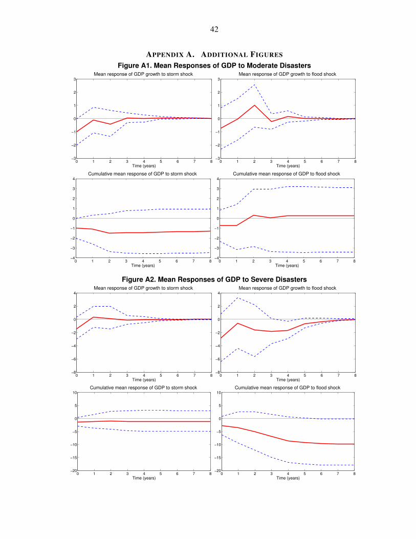
42

APPENDIX A. ADDITIONAL FIGURES

Figure A1. Mean Responses of GDP to Moderate Disasters

0 1 2 3 4 5 6 7 8−3

−2

−1

0

1

2

3

Time (years)

Mean response of GDP growth to storm shock

0 1 2 3 4 5 6 7 8−3

−2

−1

0

1

2

3

Time (years)

Mean response of GDP growth to flood shock

0 1 2 3 4 5 6 7 8−4

−3

−2

−1

0

1

2

3

4

Time (years)

Cumulative mean response of GDP to storm shock

0 1 2 3 4 5 6 7 8−4

−3

−2

−1

0

1

2

3

4

Time (years)

Cumulative mean response of GDP to flood shock

Figure A2. Mean Responses of GDP to Severe Disasters

0 1 2 3 4 5 6 7 8−8

−6

−4

−2

0

2

4

Time (years)

Mean response of GDP growth to storm shock

0 1 2 3 4 5 6 7 8−8

−6

−4

−2

0

2

4

Time (years)

Mean response of GDP growth to flood shock

0 1 2 3 4 5 6 7 8−20

−15

−10

−5

0

5

10

Time (years)

Cumulative mean response of GDP to storm shock

0 1 2 3 4 5 6 7 8−20

−15

−10

−5

0

5

10

Time (years)

Cumulative mean response of GDP to flood shock

43

Figure A3. Mean Responses of GDP and Debt to Moderate Disasters(Using Total Affected as an Alternative Measure of Intensity)

0 1 2 3 4 5 6 7 8−3

−2

−1

0

1

2

3

Time (years)

Mean response of GDP growth to storm shock

0 1 2 3 4 5 6 7 8−3

−2

−1

0

1

2

3

Time (years)

Mean response of GDP growth to flood shock

0 1 2 3 4 5 6 7 8−4

−3

−2

−1

0

1

2

3

4

Time (years)

Cumulative mean response of GDP to storm shock

0 1 2 3 4 5 6 7 8−4

−3

−2

−1

0

1

2

3

4

Time (years)

Cumulative mean response of GDP to flood shock

0 1 2 3 4 5 6 7 8−10

−5

0

5

10

Time (years)

Mean response of debt ratio growth to storm shock

0 1 2 3 4 5 6 7 8−10

−5

0

5

10

Time (years)

Mean response of debt ratio growth to flood shock

0 1 2 3 4 5 6 7 8−10

−5

0

5

10

15

Time (years)

Cumulative mean response of debt ratio to storm shock

0 1 2 3 4 5 6 7 8−10

−5

0

5

10

15

Time (years)

Cumulative mean response of debt ratio to flood shock

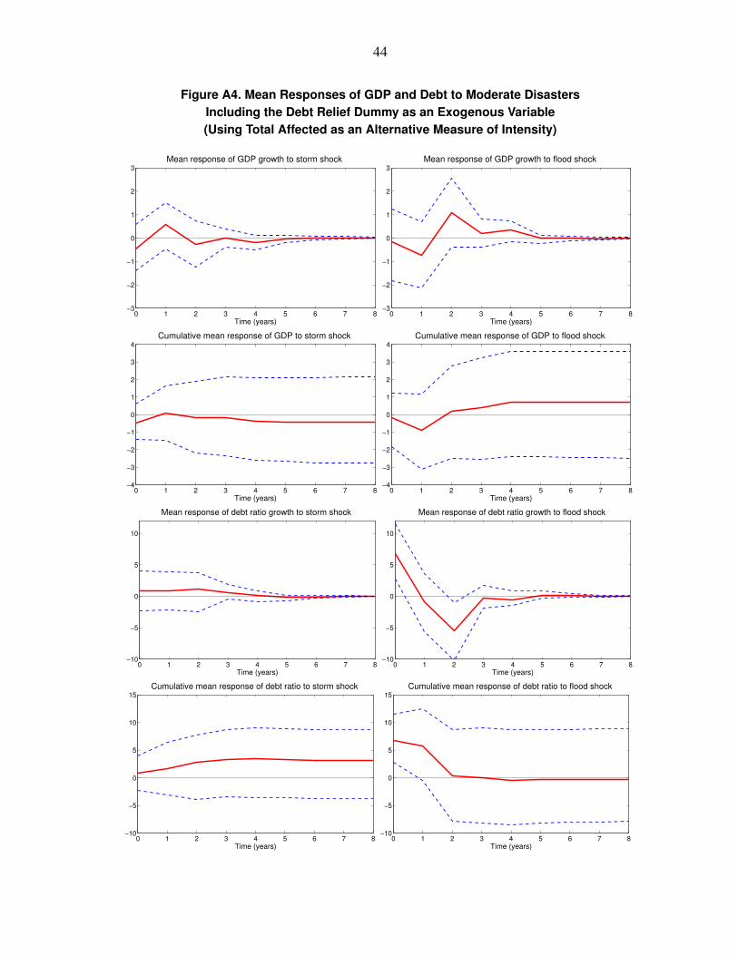
44

Figure A4. Mean Responses of GDP and Debt to Moderate DisastersIncluding the Debt Relief Dummy as an Exogenous Variable(Using Total Affected as an Alternative Measure of Intensity)

0 1 2 3 4 5 6 7 8−3

−2

−1

0

1

2

3

Time (years)

Mean response of GDP growth to storm shock

0 1 2 3 4 5 6 7 8−3

−2

−1

0

1

2

3

Time (years)

Mean response of GDP growth to flood shock

0 1 2 3 4 5 6 7 8−4

−3

−2

−1

0

1

2

3

4

Time (years)

Cumulative mean response of GDP to storm shock

0 1 2 3 4 5 6 7 8−4

−3

−2

−1

0

1

2

3

4

Time (years)

Cumulative mean response of GDP to flood shock

0 1 2 3 4 5 6 7 8−10

−5

0

5

10

Time (years)

Mean response of debt ratio growth to storm shock

0 1 2 3 4 5 6 7 8−10

−5

0

5

10

Time (years)

Mean response of debt ratio growth to flood shock

0 1 2 3 4 5 6 7 8−10

−5

0

5

10

15

Time (years)

Cumulative mean response of debt ratio to storm shock

0 1 2 3 4 5 6 7 8−10

−5

0

5

10

15

Time (years)

Cumulative mean response of debt ratio to flood shock

45

Figure A5. Mean Responses of GDP and Debt to ModerateDisasters (Using Damages as an Alternative Measure of Intensity)

0 1 2 3 4 5 6 7 8−4

−2

0

2

4

6

Time (years)

Mean response of GDP growth to storm shock

0 1 2 3 4 5 6 7 8−4

−2

0

2

4

6

Time (years)

Mean response of GDP growth to flood shock

0 1 2 3 4 5 6 7 8−5

0

5

10

Time (years)

Cumulative mean response of GDP to storm shock

0 1 2 3 4 5 6 7 8−5

0

5

10

Time (years)

Cumulative mean response of GDP to flood shock

0 1 2 3 4 5 6 7 8−25

−20

−15

−10

−5

0

5

10

15

Time (years)

Mean response of debt ratio growth to storm shock

0 1 2 3 4 5 6 7 8−25

−20

−15

−10

−5

0

5

10

15

Time (years)

Mean response of debt ratio growth to flood shock

0 1 2 3 4 5 6 7 8−40

−30

−20

−10

0

10

20

Time (years)

Cumulative mean response of debt ratio to storm shock

0 1 2 3 4 5 6 7 8−40

−30

−20

−10

0

10

20

Time (years)

Cumulative mean response of debt ratio to flood shock

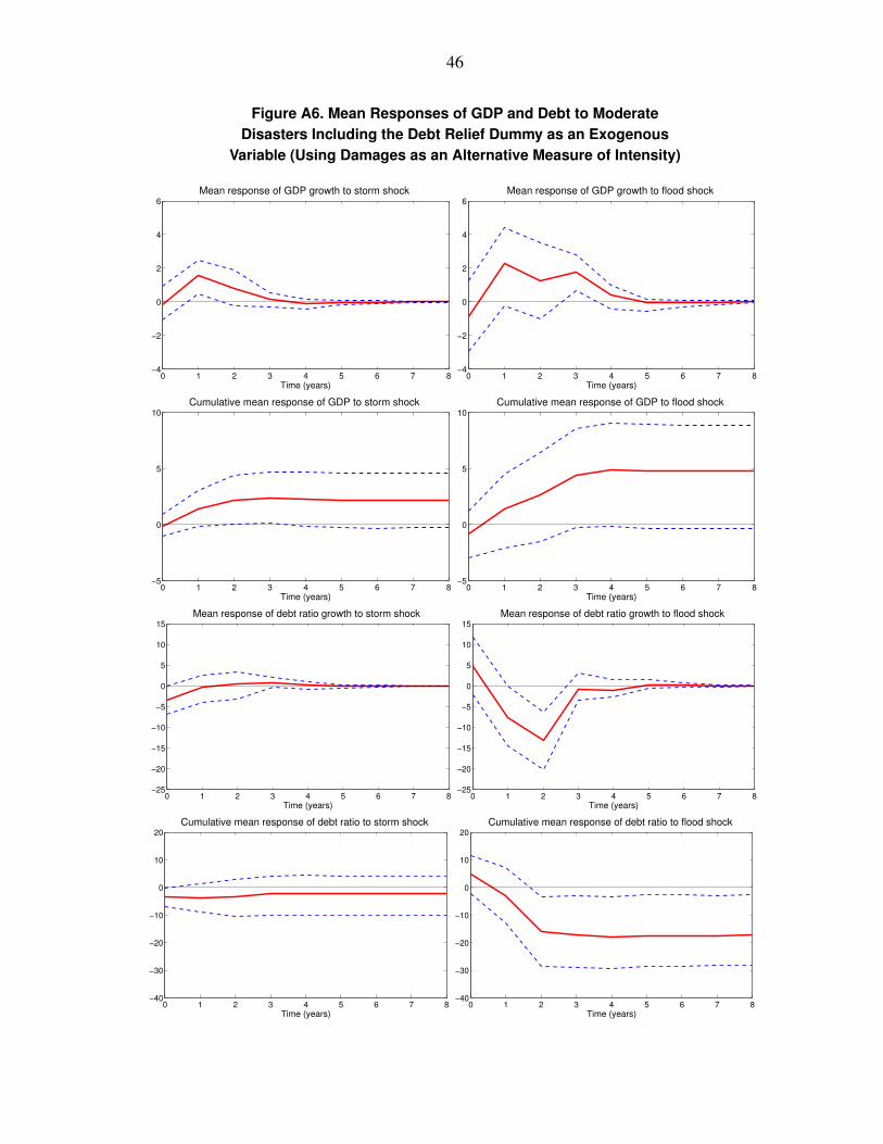
46

Figure A6. Mean Responses of GDP and Debt to ModerateDisasters Including the Debt Relief Dummy as an Exogenous

Variable (Using Damages as an Alternative Measure of Intensity)

0 1 2 3 4 5 6 7 8−4

−2

0

2

4

6

Time (years)

Mean response of GDP growth to storm shock

0 1 2 3 4 5 6 7 8−4

−2

0

2

4

6

Time (years)

Mean response of GDP growth to flood shock

0 1 2 3 4 5 6 7 8−5

0

5

10

Time (years)

Cumulative mean response of GDP to storm shock

0 1 2 3 4 5 6 7 8−5

0

5

10

Time (years)

Cumulative mean response of GDP to flood shock

0 1 2 3 4 5 6 7 8−25

−20

−15

−10

−5

0

5

10

15

Time (years)

Mean response of debt ratio growth to storm shock

0 1 2 3 4 5 6 7 8−25

−20

−15

−10

−5

0

5

10

15

Time (years)

Mean response of debt ratio growth to flood shock

0 1 2 3 4 5 6 7 8−40

−30

−20

−10

0

10

20

Time (years)

Cumulative mean response of debt ratio to storm shock

0 1 2 3 4 5 6 7 8−40

−30

−20

−10

0

10

20

Time (years)

Cumulative mean response of debt ratio to flood shock