Damage Detection with Ambient Vibration Data Using Time Series Modeling

Mustafa Gul 1, F. Necati Catbas 2

Department of Civil, Environmental and Construction Engineering

University of Central Florida, Orlando

1 mgul@mail.ucf.edu 2catbas@mail.ucf.edu

NOMENCLATURE

: Mass matrix B(q): Polynomials in the delay operator q-1

: Damping matrix C(q): Polynomials in the delay operator q-1

: Stiffness matrix q-1: Delay operator

x(t): Output of the system y(t): Output of the ARMAX model

f(t): Excitation force on the system u(t): Input to the ARMAX model A(q): Polynomials in the delay operator q-1 e(t): Error term in the ARMAX model

ABSTRACT

In this study, a novel approach using a modified time series analysis methodology is used to detect, locate, and quantify structural changes by using ambient vibration data. Random Decrement (RD) is used to obtain pseudo free response data from the ambient vibration time histories. ARX models (Auto-Regressive models with eXogenous input) are created for different sensor clusters by using the pseudo free response of the structure. The output of each sensor in a cluster is used as an input to the ARX model to predict the output of the reference channel of that sensor cluster. After the ARX models for the healthy structure for each sensor cluster are created, the same models are used for predicting the data from the damaged structure. The difference between the fit ratios is used as damage indicating feature. The methodology is applied to experimental data obtained from steel grid structure tests and it is shown that the approach is successfully used for identification, localization, and quantification of different damage cases for both impact and ambient tests.

INTRODUCTION

Structural Health Monitoring (SHM) is the research area focusing on condition assessment of different types of structures including aerospace, mechanical and civil structures. Damage detection is arguably one of the most critical components of SHM. A common approach to extract damage sensitive features (or damage features) from SHM data is to use time series analysis [1-11]. AR (Auto Regressive), ARX (Auto Regressive model with eXogenous input) and ARMA (Auto-Regressive Moving Average) models are some of the time series analysis methods employed by different researchers. One of the main advantages of such methodologies is that it requires only the data from the undamaged structure in the training phase (i.e. unsupervised learning) as opposed to supervised learning where data from both undamaged and damaged conditions is required to train the model. These types of methods have been widely studied also since their implementation for an automated SHM system is relatively more feasible compared to other methodologies such as damage detection based on model updating.

Proceedings of the IMAC-XXVIIIFebruary 1–4, 2010, Jacksonville, Florida USA

©2010 Society for Experimental Mechanics Inc.

In a recent study, the authors proposed a time series methodology where ARX models were used to model the free response of different sensor clusters for damage detection [12]. The authors showed that the method was very successful in identifying, locating and quantifying the damage with different numerical and experimental data [13, 14]. In this paper, the methodology is modified and improved for damage detection with ambient vibration data. The details of the methodology, theoretical background and experimental results are given in the following sections.

Objective and Scope

The objective of this study is to present a time series analysis methodology to identify, locate and quantify damage by using ambient vibration data. First, the theoretical background of time series modeling and its relation with structural dynamics is briefly discussed. Then the methodology is applied to different experimental datasets from a large-scale laboratory model for damage detection. Results from impact and ambient tests are presented in a comparative fashion to show the effectiveness of the approach.

THEORETICAL BACKGROUND

The equation of motion for an N Degrees of Freedom (DOF) linear dynamic system can be written as in Eqn. (1).

(1)

where is the mass matrix, is the damping matrix and is the stiffness matrix. The vectors and are acceleration, velocity and displacement, respectively. The external forcing function on the system is denoted with . The same equation can be written in matrix form as shown in Eqn. (2) (t for time is omitted). Furthermore, if the first row of this matrix equation is considered for free response case, the relation is written as shown by Eqn. (3).

(2)

(3)

It is seen from Eqn. (3) that if a model is created to predict the output of the first DOF by using the DOFs connected to it (neighbor DOFs), the change in this model can reveal important information about the change in the properties of that part of the system. Obviously, similar equalities can be written for each row of Eqn. (2) and different models can be created for each equation. Each row of Eqn. (2) can be considered as a sensor cluster with a reference DOF and its neighbor DOFs. The reference DOF for Eqn. (3), for example, is the first DOF and neighbor DOFs are the DOFs that are directly connected to the first DOF. Therefore, it is proposed that different linear time series models can be created to establish different models for each sensor cluster and changes in these models can point the existence, location and severity of the damage. The details of the methodology are explained in the following sections.

A general form of a time series model can be written as in Eqn. (4)-(5) and an ARX model is shown in Eqn. (6).

(4)

(5)

(6)

where, y(t) is the output of the model, u(t) is the input to the model and e(t) is the error term. The unknown parameters of the model are shown with ai, bi, and di and the model orders are shown with na, nb and nd.

As indicated above, Eqn. (3) can be used in the case of free response analysis. Although the free response of a structure can be easily measured for some applications, in most of the civil engineering applications it may not always be practical or easy to collect the free response data. Therefore, the authors implemented the Random Decrement (RD) Technique to obtain the pseudo free response data from the ambient vibration data [15-17].

The basic idea behind the RD is that the random response of a system at the time consists of three

components, which are the step response due to the initial displacements at the time , the impulse response

from initial velocity at time , and a random part due to the load applied to the structure between and . By taking average of time segments, every time the response has an initial displacement bigger than the trigger level given in Eqn. (7), the random part due to random load will eventually die out and become negligible. Additionally, since the sign of the initial velocity can be assumed to vary randomly in time, the resulting initial velocity will be zero.

(7)

After the pseudo-free response data is obtained by using RD, this data is used to create different ARX models for different sensor clusters. Then damage sensitive features are extracted from these models to detect the damage. In these ARX models, the y(t) term in Eqn. (6) is the acceleration response of the reference channel of a sensor cluster, while the u(t) term is defined with the acceleration responses of all the DOFs in the same cluster. Eqn. (8) shows an example ARX model to estimate the 1st DOF’s output by using the other DOFs’ outputs for a sensor cluster with k sensors.

(8)

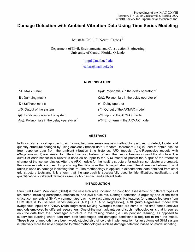
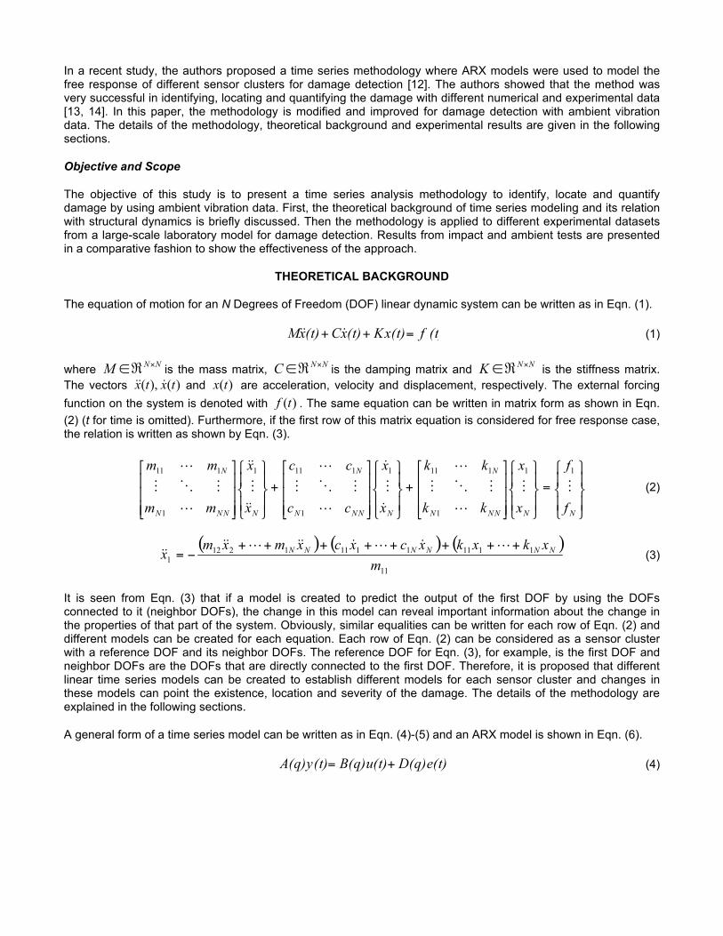
To explain the methodology schematically, a simple 3-DOF model is used as an example. Figure 1 shows the first sensor cluster for the first reference channel. The cluster includes first and second DOFs since the reference channel is connected only to the second DOF. The input vector u of the ARX model contains the acceleration outputs of first and second DOFs. The output of the first DOF is used as the output of the ARX model as shown in the figure. When the second channel is the reference channel, Figure 2, the sensor cluster includes all three DOFs since they are all connected to the second DOF. Sensor clusters for each reference channels are created with the same concept. After creating the ARX models for the baseline condition, the fit ratios of the baseline ARX model when used with new data is employed as a damage sensitive feature. Further details about the methodology and applications are discussed in Gul and Catbas [18].

Figure 1. Creating different ARX models for each sensor cluster (first sensor cluster)

Figure 2. Creating different ARX models for each sensor cluster (second sensor cluster)

After creating the ARX models for the healthy structure, the same models are used to predict the output of the damaged structure for the same sensor clusters. The difference between the fit ratios of the models is used as the DF. The Fit Ratio (FR) of an ARX model is calculated as given in Eqn. (9).

(9)

where is the measured output, is the predicted output, is the mean of and is the norm of

. The DF is calculated by using the difference between the FRs for healthy and damaged cases.

EXPERIMENTAL STUDIES AND ANALYSIS RESULTS

A steel grid structure was used for the experimental demonstration of the methodology. The physical model has two clear spans with continuous beams across the middle supports. It has two 18 ft girders (S3x5.7 steel section) in the longitudinal direction. The 3 ft transverse beam members are used for lateral stability. The grid is supported by 42 in tall columns (W12x26 steel section). The grid is shown in Figure 3 and more information about the specimen can be found in Burkett [19] and Catbas et al. [20]. The grid is instrumented with 12 accelerometers in vertical direction at each node (all the nodes except N7 to.N14). The accelerometers used for the experiments are ICP/seismic type accelerometers with a 1000 mV/g sensitivity, 0.01 to 1200 Hz frequency range and g of measurement range.

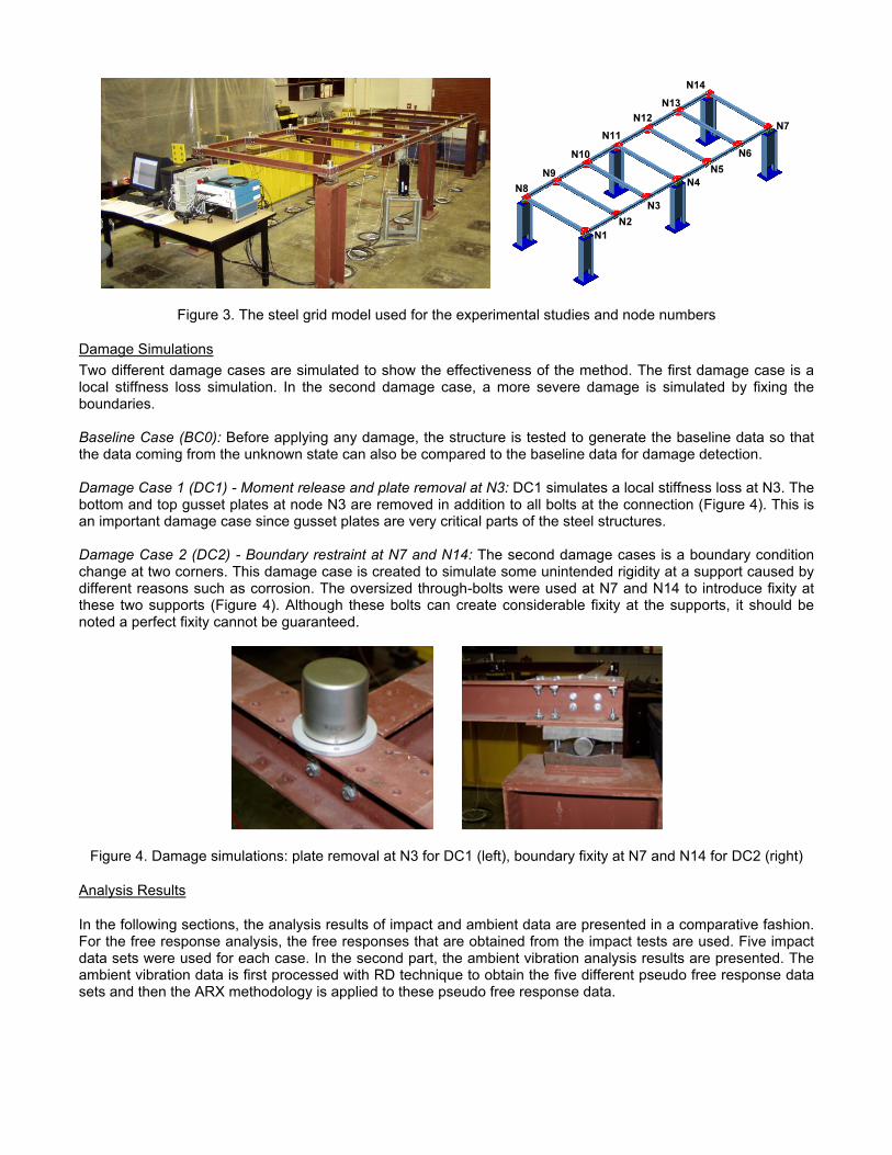
Figure 3. The steel grid model used for the experimental studies and node numbers

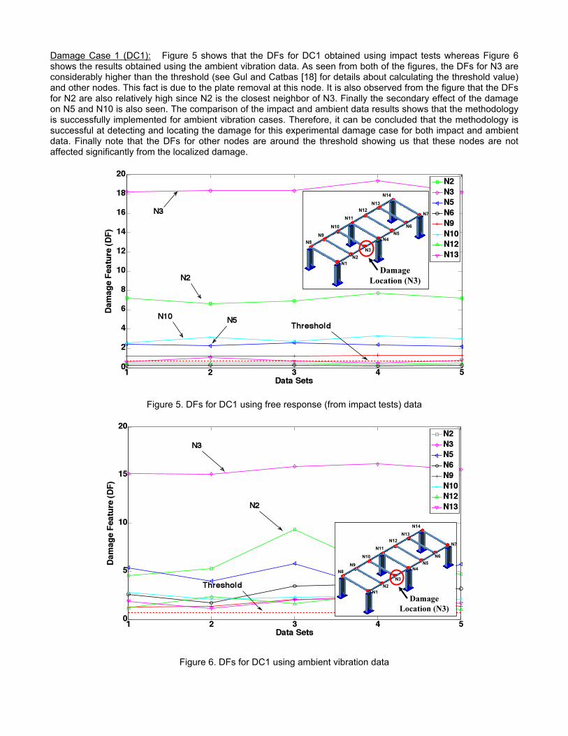
Damage Simulations Two different damage cases are simulated to show the effectiveness of the method. The first damage case is a local stiffness loss simulation. In the second damage case, a more severe damage is simulated by fixing the boundaries. Baseline Case (BC0): Before applying any damage, the structure is tested to generate the baseline data so that the data coming from the unknown state can also be compared to the baseline data for damage detection. Damage Case 1 (DC1) - Moment release and plate removal at N3: DC1 simulates a local stiffness loss at N3. The bottom and top gusset plates at node N3 are removed in addition to all bolts at the connection (Figure 4). This is an important damage case since gusset plates are very critical parts of the steel structures. Damage Case 2 (DC2) - Boundary restraint at N7 and N14: The second damage cases is a boundary condition change at two corners. This damage case is created to simulate some unintended rigidity at a support caused by different reasons such as corrosion. The oversized through-bolts were used at N7 and N14 to introduce fixity at these two supports (Figure 4). Although these bolts can create considerable fixity at the supports, it should be noted a perfect fixity cannot be guaranteed.

Figure 4. Damage simulations: plate removal at N3 for DC1 (left), boundary fixity at N7 and N14 for DC2 (right)

Analysis Results

In the following sections, the analysis results of impact and ambient data are presented in a comparative fashion. For the free response analysis, the free responses that are obtained from the impact tests are used. Five impact data sets were used for each case. In the second part, the ambient vibration analysis results are presented. The ambient vibration data is first processed with RD technique to obtain the five different pseudo free response data sets and then the ARX methodology is applied to these pseudo free response data.

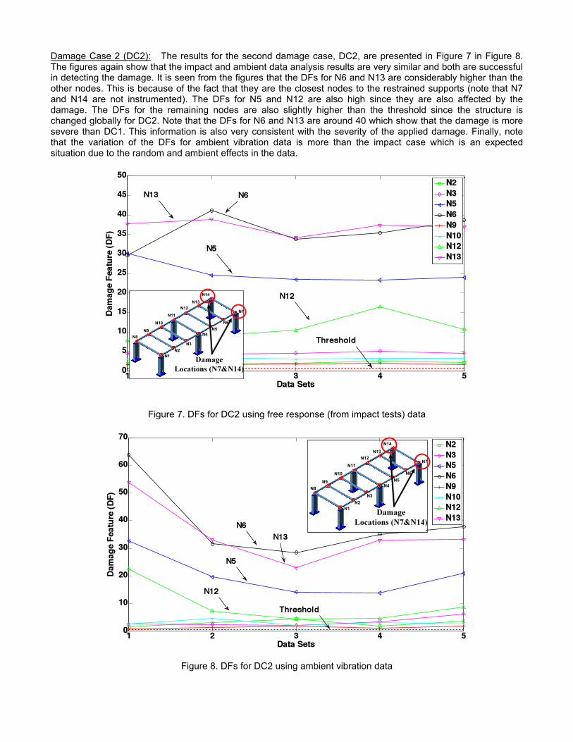
Damage Case 1 (DC1): Figure 5 shows that the DFs for DC1 obtained using impact tests whereas Figure 6 shows the results obtained using the ambient vibration data. As seen from both of the figures, the DFs for N3 are considerably higher than the threshold (see Gul and Catbas [18] for details about calculating the threshold value) and other nodes. This fact is due to the plate removal at this node. It is also observed from the figure that the DFs for N2 are also relatively high since N2 is the closest neighbor of N3. Finally the secondary effect of the damage on N5 and N10 is also seen. The comparison of the impact and ambient data results shows that the methodology is successfully implemented for ambient vibration cases. Therefore, it can be concluded that the methodology is successful at detecting and locating the damage for this experimental damage case for both impact and ambient data. Finally note that the DFs for other nodes are around the threshold showing us that these nodes are not affected significantly from the localized damage.

Figure 5. DFs for DC1 using free response (from impact tests) data

Figure 6. DFs for DC1 using ambient vibration data

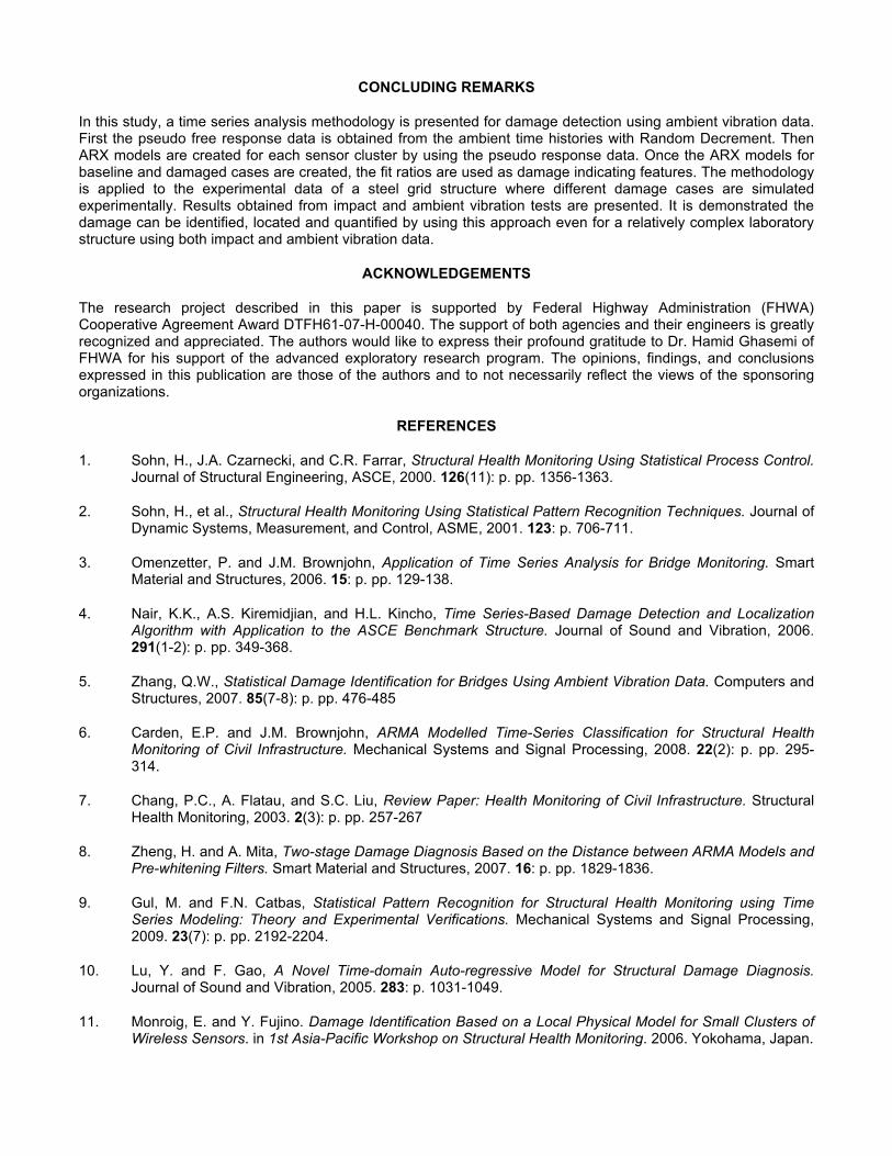
Damage Case 2 (DC2): The results for the second damage case, DC2, are presented in Figure 7 in Figure 8. The figures again show that the impact and ambient data analysis results are very similar and both are successful in detecting the damage. It is seen from the figures that the DFs for N6 and N13 are considerably higher than the other nodes. This is because of the fact that they are the closest nodes to the restrained supports (note that N7 and N14 are not instrumented). The DFs for N5 and N12 are also high since they are also affected by the damage. The DFs for the remaining nodes are also slightly higher than the threshold since the structure is changed globally for DC2. Note that the DFs for N6 and N13 are around 40 which show that the damage is more severe than DC1. This information is also very consistent with the severity of the applied damage. Finally, note that the variation of the DFs for ambient vibration data is more than the impact case which is an expected situation due to the random and ambient effects in the data.

Figure 7. DFs for DC2 using free response (from impact tests) data

Figure 8. DFs for DC2 using ambient vibration data

CONCLUDING REMARKS

In this study, a time series analysis methodology is presented for damage detection using ambient vibration data. First the pseudo free response data is obtained from the ambient time histories with Random Decrement. Then ARX models are created for each sensor cluster by using the pseudo response data. Once the ARX models for baseline and damaged cases are created, the fit ratios are used as damage indicating features. The methodology is applied to the experimental data of a steel grid structure where different damage cases are simulated experimentally. Results obtained from impact and ambient vibration tests are presented. It is demonstrated the damage can be identified, located and quantified by using this approach even for a relatively complex laboratory structure using both impact and ambient vibration data.

ACKNOWLEDGEMENTS

The research project described in this paper is supported by Federal Highway Administration (FHWA) Cooperative Agreement Award DTFH61-07-H-00040. The support of both agencies and their engineers is greatly recognized and appreciated. The authors would like to express their profound gratitude to Dr. Hamid Ghasemi of FHWA for his support of the advanced exploratory research program. The opinions, findings, and conclusions expressed in this publication are those of the authors and to not necessarily reflect the views of the sponsoring organizations.

REFERENCES

1. Sohn, H., J.A. Czarnecki, and C.R. Farrar, Structural Health Monitoring Using Statistical Process Control. Journal of Structural Engineering, ASCE, 2000. 126(11): p. pp. 1356-1363.

2. Sohn, H., et al., Structural Health Monitoring Using Statistical Pattern Recognition Techniques. Journal of Dynamic Systems, Measurement, and Control, ASME, 2001. 123: p. 706-711.

3. Omenzetter, P. and J.M. Brownjohn, Application of Time Series Analysis for Bridge Monitoring. Smart Material and Structures, 2006. 15: p. pp. 129-138.

4. Nair, K.K., A.S. Kiremidjian, and H.L. Kincho, Time Series-Based Damage Detection and Localization Algorithm with Application to the ASCE Benchmark Structure. Journal of Sound and Vibration, 2006. 291(1-2): p. pp. 349-368.

5. Zhang, Q.W., Statistical Damage Identification for Bridges Using Ambient Vibration Data. Computers and Structures, 2007. 85(7-8): p. pp. 476-485

6. Carden, E.P. and J.M. Brownjohn, ARMA Modelled Time-Series Classification for Structural Health Monitoring of Civil Infrastructure. Mechanical Systems and Signal Processing, 2008. 22(2): p. pp. 295-314.

7. Chang, P.C., A. Flatau, and S.C. Liu, Review Paper: Health Monitoring of Civil Infrastructure. Structural Health Monitoring, 2003. 2(3): p. pp. 257-267

8. Zheng, H. and A. Mita, Two-stage Damage Diagnosis Based on the Distance between ARMA Models and Pre-whitening Filters. Smart Material and Structures, 2007. 16: p. pp. 1829-1836.

9. Gul, M. and F.N. Catbas, Statistical Pattern Recognition for Structural Health Monitoring using Time Series Modeling: Theory and Experimental Verifications. Mechanical Systems and Signal Processing, 2009. 23(7): p. pp. 2192-2204.

10. Lu, Y. and F. Gao, A Novel Time-domain Auto-regressive Model for Structural Damage Diagnosis. Journal of Sound and Vibration, 2005. 283: p. 1031-1049.

11. Monroig, E. and Y. Fujino. Damage Identification Based on a Local Physical Model for Small Clusters of Wireless Sensors. in 1st Asia-Pacific Workshop on Structural Health Monitoring. 2006. Yokohama, Japan.

12. Gul, M. and F.N. Catbas. A New Methodology for Identification, Localization and Quantification of Damage by Using Time Series Modeling. in 26th International Modal Analysis Conference (IMAC XXVI). 2008. Orlando, FL.

13. Gul, M. and F.N. Catbas, A Novel Time Series Analysis Methodology for Damage Assessment, in The Fifth International Workshop on Advanced Smart Materials and Smart Structures Technology, ANCRISST 2009. 2009: Boston, MA.

14. Gul, M. and F.N. Catbas. A Modified Time Series Analysis for Identification, Localization, and Quantification of Damage. in 27th International Modal Analysis Conference (IMAC XXVII). 2009. Orlando, FL.

15. Cole, H.A., On-The-Line Analysis of Random Vibrations. American Institute of Aeronautics and Astronautics, 1968. 68(288).

16. Asmussen, J.C., Modal Analysis Based on the Random Decrement Technique-Application to Civil Engineering Structures. 1997, University of Aalborg: Aalborg.

17. Gul, M. and F.N. Catbas, Ambient Vibration Data Analysis for Structural Identification and Global Condition Assessment. Journal of Engineering Mechanics, 2008. 134(8): p. pp. 650-662.

18. Gul, M. and F.N. Catbas, Structural Health Monitoring and Damage Assessment using a Novel Time Series Analysis Methodology with Sensor Clustering. Journal of Sound and Vibration, 2009. (Under Review).

19. Burkett, J.L., Benchmark Studies for Structural Health Monitoring using Analytical and Experimental Models, in Department of Civil and Environmental Engineering. 2005, University of Central Florida: Orlando, FL.

20. Catbas, F.N., M. Gul, and J.L. Burkett, Damage Assessment Using Flexibility and Flexibility-Based Curvature for Structural Health Monitoring. Smart Materials and Structures, 2008. 17(1): p. 015024 (12 pp).