crossflow stability and transition i experiments in a ... · crossflow stabilityand transition _i...
TRANSCRIPT
b f
NASA- TM- I08_50 i,' _/'; ,
/ /f
CROSSFLOW STABILITY AND TRANSITION _iEXPERIMENTS IN A SWEPT-WING FLOW
by
J. Ray Dagenhart
Dissertation submitted to the Faculty
of the Virginia Polytechnic Institute and State University
in partial fulfillment of the requirements for the degree of
Doctor of Philosophy
in
Engineering Mechanics
Dr. W. S. Saric, Co-chairman
Dr. M. Cramer
Dr. D. Frederick
APPROVED:
Dr. W. Devenport
Dr. D. T. Mook
December 1992
Biacksburg, Virginia
(NASA-TM-I08650) CROSSFLOWSTABILITY AND TRANSITION
EXPERIMENTS IN A SWEPT-WING FLOW
Ph.O. Thesis (Virginia Polytechnic
Inst. and State Univ.) 286 p
N93-ZI819
Unclas
G3/34 0150569
https://ntrs.nasa.gov/search.jsp?R=19930012630 2020-03-31T20:03:04+00:00Z
ABSTRACT
CROSSFLOW STABILITY AND TRANSITIONEXPERIMENTS IN A SWEPT-WING FLOW
J. Ray Dagenhart
An experimental examination of crossflow instability and transition on a 45 °
swept wing is conducted in the Arizona State University Unsteady Wind Tun-
nel. The stationary-vortex pattern and transition location are visualized using
both sublimating-chemical and liquid-crystal coatings. Extensive hot-wire mea-
surements are conducted at several measurement stations across a single vortex
track. The mean and travelling-wave disturbances are measured simultaneously.
Stationary-crossflow disturbance profiles are determined by subtracting either a
reference or a span-averaged velocity profile from the mean-velocity data. Mean,
stationary-crossflow, and travelling-wave velocity data are presented as local
boundary-layer profiles and as contour plots across a single stationary-crossflow
vortex track. Disturbance-mode profiles and growth rates are determined. The
experimental data are compared to predictions from linear stability theory.
Comparison of measured and predicted pressure distributions shows that a
good approximation of infinite swept-wing flow is achieved. A fixed-wavelength
vortex pattern is observed throughout the visualization range. The theoretically-
predicted maximum-amplified vortex wavelength is found to be approximately
25% larger than the observed wavelength. Linear-stability computations for the
dominant stationary-crossflow vortices show that the N-factors at transition ranged
from 6.4 to 6.8.
The mean-velocity profiles vary slightly across the stationary-crossflow vor-
tex at the first measurement station. The variation across the vortex increases
with downstream distance until nearly all of the profiles become highly-distorted
S-shaped curves. Local stationary-crossflow disturbance profiles having either
purely excess or deficit values develop at the upstream measurement stations.
Further downstream the profiles take on crossover shapes not anticipated by
the linear theory. The maximum streamwise stationary-crossflow velocity dis-
turbances reach ±20% of the edge velocity just before transition. The travelling-
wave disturbances have single lobes at the upstream measurement stations as
expected, but further downstream double-lobed travelling-wave profiles develop.
The maximum disturbance intensity remains quite low until just ahead of the tran-
sition location where it suddenly peaks at 0.7% of the edge velocity and then drops
sharply. The travelling-wave intensity is always more than an order of magnitude
lower than the stationary crossflow-vortex strength.
The mean streamwise-velocity contours are nearly flat and parallel to the
model surface at the first measurement station. Further downstream, the contours
rise up and begin to roll over like a wave breaking on the beach. The stationary-
crossflow contours show that a plume of low-velocity fluid rises near the center
of the wavelength while high-velocity regions develop near the surface at each
end of the wavelength. There is no distinct pattern to the low-intensity travelling-
wave contours until a short distance upstream of the transition location where the
travelling-wave intensity suddenly peaks near the center of the vortex and then
falls abruptly.
The experimental disturbance-mode profiles agree quite well with the predicted
eigenfunctions for the forward measurement stations. At the later stations, the
experimental mode profiles assume double-lobed shapes with maxima above and
below the single maximum predicted by the linear theory. The experimental growth
rates are found to be less than or equal to the predicted growth rates from the linear
theory. Also, the experimental growth rate curve oscillates over the measurement
range whereas the theoretically-predicted growth rates decrease monotonically.
ACKNOWLEDGMENTS
The author is sincerely grateful to Dr. William S. Saric for his invaluable advice,
support, encouragement, and patience as the dissertation advisor. Special thanks
go to Dr. Helen L. Reed who provided theoretical data for comparison with the
experimental results and Dr. W. Pfenninger who continually provided technical
insight and discussion throughout the project.
The author also thanks Dr. Demetri Telionis for acting as the examining
committee co-chairman and Drs. Daniel Frederick, Dean T. Mook, Mark Cramer,
and William Devenport for acting as members of the examining committee. Mr. W.
D. Harvey and Dr. Stephen K. Robinson, my former and present branch heads at
NASA Langley Research Center, gave necessary support and encouragement.
Messrs. Jon Hoos, Marc Mousseux, Ronald Radeztsky, and Dan Clevenger
provided important assistance and valuable discussion of the research at the
Unsteady Wind Tunnel. Thanks are extended to Messrs. Harry L. Morgan and
J. P. Stack of NASA Langley for assistance in computational and measurement
aspects of the research. Finally, technical discussions with many members of the
Experimental Flow Physics Branch contributed significantly to the work.
I am forever grateful to my parents, John and Anne Dagenhart, for their
continuing support and encouragement throughout my educational career.
I also gratefully acknowledge the understanding, encouragement, and pa-
tience of my good friend, Malinda Knight.
J,¥
PREeEl)ii',iG PIIt',._,CBLAI_.;K i',lOi" FiL_'IED
Contents
ABSTRACT ........................................ ii
ACKNOWLEDGMENTS ................................. iv
List of Tables ........................................ vii
List of Figures ....................................... ix
1 INTRODUCTION .................................. 1
1.1 Background ................................... 1
1.2 Instability Modes ................................ 4
1.3 Goals of the Present Investigation ..................... 4
1.4 Outline ...................................... 5
2 REVIEW OF SWEPT-WING FLOWS ...................... 7
2.1 Stability and Transition Prediction ..................... 7
2.2 Transition Experiments ............................ 10
2.3 Detailed Theory and Simulation ...................... 11
2.4 Stability Experiments ............................. 13
2.5 State of Present Knowledge ......................... 15
3 EXPERIMENTAL FACILITY ............................ 17
3.1 ASU Unsteady Wind Tunnel ......................... 17
3.2 New Test Section ............................... 19
4 MODEL AND LINER DESIGN .......................... 21
4.1 Airfoil Selection ................................. 21
4.1.1 Pressure Gradient Effects ....................... 21
4.1.2 Wind-Tunnel Wall Interference Effects ................ 24
4.2 Stability Calculations ............................. 25
4.2.1
4.2.2
4.2.3
4.2.4
4.3
4.4
4.5
Stationary Crossflow Vortices ..................... 27
Tollmien-Schlichting Waves ...................... 29
Travelling Crossflow Vortices ..................... 30
Crossflow/Tollmien-Schlichting Interaction ............. 32
Selection of the Experimental Test Condition .............. 33
Reynolds Number Variation ......................... 34
Test-Section Liner Shape .......................... 34
5 EXPERIMENTAL RESULTSAND DISCUSSION .............. 395.1 Freestream Flow Quality ........................... 395.2 Pressure Distributions ............................ 405.3 Flow Visualizations .............................. 415.4 Transition Locations .............................. 435.5 Boundary-Layer Spectra ........................... 445.6 Boundary-Layer Hot-Wire Surveys ..................... 45
5.6.1 Streamwise-Velocity Measurements ................. 455.6.2 Spanwise Variation of Streamwise Velocity ............. 485.6.3 Disturbance Profiles ........................... 495.6.4 Streamwise-Velocity Contour Plots .................. 53
5.7 Experimental/TheoreticalComparisons .................. 595.7.1 Theoretical Disturbance Profiles ................... 605.7.2 Disturbance Profile Comparisons ................... 625.7.3 Comparison of Experimental Streamwise Velocity-Contour
Plots and Theoretical Vector Plots ................. 645.7.4 Wavelength Comparison ........................ 665.7.5 Growth Rate Comparison ........................ 67
5.8 Experimental Results Summary ...................... 686 CONCLUSIONS ................................... 77Appendix A Relationships Between Coordinate Systems .......... 247Appendix B Hot-Wire Signal InterpretationProcedure ............ 251Appendix C Error Analysis ............................ 255References ........................................ 261
vi
List of Tables
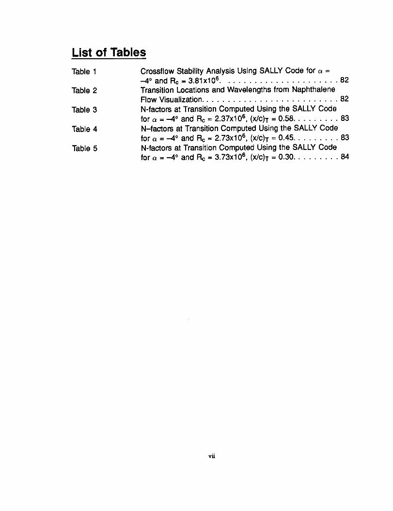
Table 1
Table 2
Table 3
Table 4
Table 5
Crossflow Stability Analysis Using SALLY Code for a =-4 ° and Rc = 3.81x10⁶ ...................... 82Transition Locations and Wavelengths from NaphthaleneFlow Visualization .......................... 82N-factors at Transition Computed Using the SALLY Codefor a = -40 and Rc = 2.37x10⁶, (X/C)T = 0.58 ......... 83N-factors at Transition Computed Using the SALLY Codefor a = -40 and Rc = 2.73x10⁶, (x/C)T = 0.45 ......... 83N-factors at Transition Computed Using the SALLY Codefor a = -40 and Rc = 3.73xl 06, (x/C)T = 0.30 ......... 84
vfi

List of Figures
Figure 1Figure 2Figure 3
Figure 4
Figure 5Figure 6
Figure 7
Figure 8
Figure 9
Figure 10
Figure 11
Figure 12
Figure 13
Figure 14
Figure 15
Figure 16
Figure 17
Figure 18
Figure 19
Figure 20
Figure 21
Curved Streamlines over a Swept Wing ............ 85Boundary-Layer Velocity Profiles on a Swept Wing ..... 86Plan View of Arizona State University Unsteady WindTunnel (Dimensions in meters) ................. 87Photograph of New UWT Test Section With Liner UnderConstruction ............................. 88
NLF(2)-0415 Airfoil ......................... 89NLF(2)-0415 Design Point Pressure Distribution at o_= 0 °and 6f = 0 ° in Free Air. ...................... 90NLF(2)-0415 Pressure Distribution for o_= -40 and @ = 0°in Free Air .............................. 91
NLF(2)°0415 Pressure Distribution for _ = -2 ° and _f = 0°in Free Air .............................. 92NLF(2)-0415 Pressure Distribution for e = 20 and @ = 0°in Free Air .............................. 93NLF(2)-0415 Pressure Distribution for a = 4° and _f = 0°in Free Air .............................. 94NLF(2)-0415 Pressure Distribution for c_= 0 ° and _f =-20 ° in Free Air ........................... 95
NLF(2)-0415 Pressure Distribution for oL= 0 ° and <_f=-10 ° in Free Air ........................... 96
NLF(2)-0415 Pressure Distribution for a -- 0 ° and 6f = 10°_n Free Air .............................. 97NLF(2)-0415 Pressure Distribution for _ = 0 ° and 6f = 20 °in Free Air .............................. 98
NLF(2)-0415 Pressure Distribution for _ = -40 and 6f = 0 °in UWT ................................ 99
NLF(2)-0415 Pressure Distribution for _ = -20 and @ = 0 °in UWT ............................... 100
NLF(2)-0415 Pressure Distribution for e = 0 ° and @ = 0 °m UWT ............................... 101NLF(2)-0415 Pressure Distribution for _ = 20 and <_f= 0 °zn UWT ............................... 102
NLF(2)-0415 Pressure Distribution for o_-- 4 ° and 6f = 0 °in UWT ............................... 103
Local Spatial Growth Rates for Stationary CrossflowVortices at _ = -40 and _f -- 0 ° in UWT, Rc = 3.81 xl0 e. . 104Local Spatial Growth Rates for Stationary CrossflowVortices at _ = -20 and _f -= 0 ° in UWT, Rc = 3.81x10⁶. . 105
ix
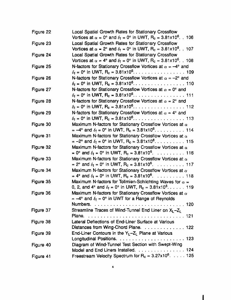
Figure 22
Figure 23
Figure 24
Figure 25
Figure 26
Figure 27
Figure 28
Figure 29
Figure 30
Figure 31
Figure 32
Figure 33
Figure 34
Figure 35
Figure 36
Figure 37
Figure 38
Figure 39
Figure 40
Figure 41
Local Spatial Growth Rates for Stationary Cross/lowVortices at c_= 0 ° and _f -- 0° in UWT, Rc = 3.81xl 06. . 106Local Spatial Growth Rates for Stationary CrossflowVortices at e = 2 ° and &f = 0° in UWT, Rc = 3.81x10⁶. . 107Local Spatial Growth Rates for Stationary Cross/lowVortices at _ = 4 ° and _f = 0° in UVVT, Rc = 3.81x10⁶. . 108N-factors for Stationary Cross/low Vortices at _ = -40 and_f = 0° in UWT, Rc = 3.81x10⁶ ................. 109N-factors for Stationary Cross/low Vortices at o_= -2 ° and6f = 0° in UWT, Rc = 3.81x10 s................. 110N-factors for Stationary Cross/low Vortices at _ = 0° and_f = 0° in UWT, Rc = 3.81x10⁶ ................. 111N-factors for Stationary Cross/low Vortices at _ = 2° and_f = 0° in UWT, Rc = 3.81x10⁶ ................. 112N-factors for Stationary Cross/low Vortices at _ = 4 ° and&f = 0° in UWT, Rc = 3.81 x10⁶ ................. 113
Maximum N-factors for Stationary Crossflow Vortices atxl0 .......... 114= -40 and _f = 0° in UWT, Rc = 3.81 6
Maximum N-factors for Stationary Crossflow Vortices atxl0 .......... 115= -2 ° and _f = 0° in UWT, Rc = 3.81 6
Maximum N-factors for Stationary Crossflow Vortices at o_= 0° and 6f = 0° in UWq', Rc = 3.81x10⁶ .......... 116
Maximum N-factors for Stationary Crossflow Vortices at= 2° and 6f = 0° in UWT, Rc = 3.81x10 s.......... 117Max=mum N-factors for Stationary Crossflow Vortices at o,= 40 and 6f = 0° in UWq', Rc = 3.81 x10⁶ .......... 118Maximum N-factors for Tollmien-Schlichting Waves for _ =0, 2, and 40 and _f = 0 ° in UWT, Rc = 3.81x10⁶ ...... 119Maximum N-factors for Stationary Crossflow Vortices at o,= -40 and _f = 0° in UWT for a Range of ReynoldsNumbers .............................. 120
Streamline Traces of Wind-Tunnel End Liner on XL-Z L
Plane ................................ 121Lateral Deflections of End-Liner Surface at VariousDistances from Wing-Chord Plane .............. 122End-Liner Contours in the YL--ZL Plane at VariousLongitudinal Positions ...................... 123Diagram of Wind-Tunnel Test Section with Swept-WingModel and End Liners Installed ................ 124Freestream Velocity Spectrum for Rc = 3.27x10⁶ ..... 125
Figure 42
Figure 43
Figure 44
Figure 45
Figure 46
Figure 47
Figure 48
Figure 49
Figure 50Figure 51Figure 52
Figure 53
Figure 54
Figure 55
Figure 56
Figure 57
Figure 58
Figure 59
Figure 60
Figure 61
Figure 62
Comparison of Measured and Predicted Model PressureCoefficients at the Upper End of the Model, a = -4 °. . . 126Comparison of Measured and Predicted Model PressureCoefficients at the Lower End of the Model, o_= -40... 127
Naphthalene Flow Visualization, a = -40, Rc =1.93x10 s.............................. 128
Naphthalene Flow Visualization, a = -40, Rc =2.19x10⁶ .............................. 129
Naphthalene Flow Visualization, a = -40, Rc =2.40xl 0s.............................. 130
Naphthalene Flow Visualization, a = -40, Rc =2.73x 10⁶ .............................. 131
Naphthalene Flow Visualization, a - -40, Rc =3.27xl 06.............................. 132
Naphthalene Flow Visualization Showing Vortex Tracks inthe Turbulent Regions ...................... 133Liquid-crystal Flow Visualization ................ 134Transition Location Versus Reynolds Number ....... 135Boundary-Layer Velocity Spectrum, a = -40, Rc =2.62x 10⁶ .............................. 136
Boundary-Layer Velocity Spectrum, ot = -40, Rc =2.82xl 06.............................. 137
Boundary-Layer Velocity Spectrum, a = -40, Rc =2.92x 10⁶ .............................. 138
Boundary-Layer Velocity Spectrum, a -- -40, Rc =3.28x 10⁶ .............................. 139
Comparison of Measured and Predicted Boundary-LayerVelocity Spectra, a = -40, Rc = 2.92xl 0 s.......... 140Streamwise-Velocity Profiles at x/c = 0.20, o_= -4 °, Rc =2.37x 10⁶ .............................. 141
Streamwise-Veiocity Profiles at x/c = 0.25, o_= -40, Rc =2.37x 10⁶ .............................. 142
Streamwise-Velocity Profiles at x/c = 0.30, o_= -40, Rc =2.37x 10⁶ .............................. 143
Streamwise-Velocity Profiles at x/c = 0.35, o_= -40, Rc =2.37xl 06 .............................. 144
Streamwise-Velocity Profiles at x/c = 0.40, a = -40, Rc =2.37xl 06.............................. 145
Streamwlse-Velocity Profiles at x/c = 0.45 a = -40, Rc =2.37xl 06 .............................. 146
xi

Figure 63
Figure 64
Figure 65
Figure 66
Figure 67
Figure 68
Figure 69
Figure 70
Figure 71
Figure 72
Figure 73
Figure 74
Figure 75
Figure 76
Figure 77
Figure 78
Figure 79
Figure 80
Figure 81
Figure 82
Streamwise-Velocity Profiles at x/c = 0.50, _ = -4 °, Rc =2.37x 10⁶ .............................. 147
Streamwise-Velocity Profiles at x/c = 0.55, _ = -40, Rc =2.37x 10s.............................. 148
Stationary Crossflow-Disturbance Velocity Profiles at x/c =0.20 a = -4o, Rc = 2.37x10⁶ Obtained From Us - Us avg. 149Stationary Crossflow-Disturbance Velocity Profiles at x/c =0.25 o_= -4o, Rc = 2.37x10⁶ Obtained From Us - Us avg. 150Stationary Crossflow-Disturbance Velocity Profiles at x/c =0.30 e =-4°, Rc = 2.37x10⁶ Obtained From Us - Us avg. 151Stationary Crossflow-Disturbance Velocity Profiles at x/c =0.35 e = -40, Rc = 2.37x10⁶ Obtained From Us - Us avg. 152Stationary Crossflow-Disturbance Velocity Profiles at x/c =0.40 a = -4o, Rc = 2.37x10⁶ Obtained From Us - Us avg. 153Stationary Crossflow-Disturbance Velocity Profiles at x/c =0.45 a = -40 Rc = 2.37xl 06 Obtained From Us - Us avg. 154Stationary Crossflow-Disturbance Velocity Profiles at x/c =0.50 a = -40, Rc = 2.37x10⁶ Obtained From Us - Us avg. 155Stationary Crossflow-Disturbance Velocity Profiles at x/c =0.55 c_= -4 °, Rc = 2.37x10⁶ Obtained From Us - Us avg. 156Stationary Crossflow-Disturbance Velocity Profiles at x/c =0.20 o_= -40, Rc = 2.37x10⁶ Obtained From Us - Us ref. 157Stationary Crossflow-Disturbance Velocity Profiles at x/c =0.25 c_=-4°, Rc = 2.37x10⁶ Obtained From Us - Us rof. 158Stationary Crossflow-Disturbance Velocity Profiles at x/c =0.30, c==-4°, Rc = 2.37x10⁶ Obtained From Us - Us rof. 159Stationary Crossflow-Disturbance Velocity Profiles at x/c =0.35, _ =-4°, Rc = 2.37x10⁶ Obtained From Us - Us ref. 160Stationary Crossflow-Disturbance Velocity Profiles at x/c =0.40, a =-4°, Rc = 2.37x10⁶ Obtained From Us - Us ref. 161Stationary Crossflow-Disturbance Velocity Profiles at x/c =0.45, _ = -40, Rc = 2.37x10⁶ Obtained From Us - Us rof. 162Stationary Crossflow-Disturbance Velocity Profiles at x/c =0.50, a = -4o, Rc = 2.37x10⁶ Obtained From Us - Us ref. 163Stationary Crossflow-Disturbance Velocity Profiles at x/c =0.55, _ =-4°, Rc = 2.37x10⁶ Obtained From Us - Us ref- 164Travelling Wave Disturbance Velocity Profiles for f = 100Hz at x/c = 0.20, a = -4o, Rc = 2.37x10⁶ .......... 165
Travelling Wave Disturbance Velocity Profiles for f = 100Hz at x/c = 0.25, _ = -4o, Rc = 2.37xl 06.......... 166
xiJ

Figure 83
Figure 84
Figure 85
Figure 86
Figure 87
Figure 88
Figure 89
Figure 90
Figure 91
Figure 92
Figure 93
Figure 94
Figure 95
Figure 96
Figure 97
Figure 98
Figure 99
Figure 1O0
Figure 101
Figure 102
Travelling Wave Disturbance Velocity Profiles for f = 100Hz at x/c = 0.30, a = -4 °, Rc = 2.37x10 s.......... 167Travelling Wave Disturbance Velocity Profiles for f = 100Hz at x/c = 0.35, a = -40, Rc = 2.37xl 06 .......... 168Travelling Wave Disturbance Velocity Profiles for f = 100Hz at x/c = 0.40, a = -4 °, Rc = 2.37x10⁶ .......... 169
Travelling Wave Disturbance Velocity Profiles for f = 100Hz at x/c = 0.45, a = -40, Rc = 2.37xl 06 .......... 170Travelling Wave Disturbance Velocity Profiles for f = 100Hz at x/c = 0.50, e = -40 Rc = 2.37x10 s.......... 171
Travelling Wave Disturbance Velocity Profiles for f = 100Hz at x/c = 0.55, e = -4o, Rc = 2.37x10⁶ .......... 172Mean Streamw=se-Velocity Contours at x/c = 0.20 e =-40, Rc = 2.37x10⁶ ........................ 173Mean Streamw=se-Velocity Contours at x/c = 0.25 ot =-40, Rc = 2.37x10⁶ ........................ 174Mean Streamwise-Velocity Contours at x/c = 0.30 _ =-40, Rc = 2.37x10 s........................ 175
Mean Streamw=se-Velocity Contours at x/c = 0.35 a =-40, Rc = 2.37x10⁶ ........................ 176Mean Streamwise-Velocity Contours at x/c = 0.40 _ =-40 Rc = 2.37x10⁶ ........................ 177Mean Streamwise-Velocity Contours at x/c = 0.45 a =-4o, Rc = 2.37x10⁶ ........................ 178
Mean Streamwtse-Velocity Contours at x/c = 0.50 _ =-40, Rc = 2.37x10⁶ ........................ 179Mean Streamwise-Velocity Contours at x/c = 0.55 _ =-40, Rc = 2.37x10⁶ ........................ 180Stationary Crossflow-Vortex Velocity Contours ObtainedFrom Us - Us avg at x/c = 0.20 _ = -40, Rc = 2.37x10⁸. 181Stationary Crossflow-Vortex Velocity Contours ObtainedFrom Us - Us avgat x/c = 0.25 a = -4 °, Rc = 2.37x10⁶. 182Stationary Crossflow-Vortex Velocity Contours ObtainedFrom Us - Us avgat x/c = 0.30 _ = -4 °, Rc = 2.37x10 s. 183Stationary Crossflow-Vortex Velocity Contours ObtainedFrom Us - Us avgat xJc = 0.35 oz= -4o, Rc = 2.37x10⁶. 184Stationary Crossflow-Vortex Velocity Contours ObtainedFrom Us - Us avgat xJc= 0.40, c_= --4°, Rc = 2.37x10⁶. 185Stationary Crossflow-Vortex Velocity Contours ObtainedFrom Us - Us avgat x/c = 0.45, a, = -4 °, Rc = 2.37x10⁸. 186
,°°X3.U
Figure 103
Figure 104
Figure 105
Figure 106
Figure 107
Figure 108
Figure 109
Figure 110
Figure 111
Figure 112
Figure 113
Figure 114
Figure 115
Figure 116
Figure 117
Figure 118
Figure 119
Figure 120
Figure 121
Figure 122
Stationary Crossflow-Vortex Velocity Contours ObtainedFrom Us - Us avg at x/c = 0.50, a = -4 °, Rc = 2.37xl 06. . 187Stationary Crossflow-Vortex Velocity Contours ObtainedFrom Us - Us avgat x/c = 0.55, o_= -4 °, Rc = 2.37xl 06. . 188Stationary Crossflow-Vortex Velocity Contours ObtainedFrom Us - Us rof at x/c = 0.20, ot = -40, Rc = 2.37x10⁶. . 189Stationary Crossflow-Vortex Velocity Contours ObtainedFrom Us - Us ref at x/c = 0.25, a = -40, Rc = 2.37x10⁶. . 190
Stationary Crossflow-Vortex Velocity Contours ObtainedFrom Us - Us ref at x/c = 0.30 a = -40, Rc = 2.37x10⁶. 191Stationary Crossflow-Vortex Velocity Contours ObtainedFrom Us - Us ref at x/c = 0.35, a = -40, Rc = 2.37x10⁶. 192Stationary Crossflow-Vortex Velocity Contours ObtainedFrom Us - Us rof at x/c -- 0.40 a = -4o, Rc = 2.37x10⁶. 193Stationary Crossflow-Vortex Velocity Contours ObtainedFrom Us - Us ref at xJc = 0.45 _ = -40, Rc = 2.37x10⁶. 194
Stationary Crossflow-Vortex Velocity Contours ObtainedFrom Us - Us rofat x/c = 0.50, ot -- -40, Rc = 2.37x10⁶. 195Stationary Crossflow-Vortex Velocity Contours ObtainedFrom Us - Us ref at x/c -- 0.55, c_= -40, Rc = 2.37x10⁶. 196Travelling-Wave RMS-Velocity Contours for f = 100 Hz atx/c -- 0.20, a = -40, Rc = 2.37x10⁶ .............. 197Travelling-Wave RMS-Velocity Contours for f = 100 Hz atx/c = 0.25, a = -40, Rc = 2.37x10⁶ .............. 198
Travelling-Wave RMS-Velocity Contours for f = 100 Hz atx/c = 0.30, a = -4 ° Rc = 2.37x10⁶ .............. 199
Travelling-Wave RMS-Velocity Contours for f = 100 Hz atx/c = 0.35 o_= -40 Rc = 2.37x10⁶ .............. 200Travelling-Wave RMS-Velocity Contours for f = 100 Hz atx/c = 0.40 a = -40 Rc = 2.37x10⁶ .............. 201
Travelling-Wave RMS-Velocity Contours for f = 100 Hz atx/c = 0.45 a = -40, Rc = 2.37x10⁶ .............. 202
Travelling-Wave RMS-Velocity Contours for f = 100 Hz atx/c = 0.50 a = -4o, Rc = 2.37x10⁶ .............. 203
Travelling-Wave RMS-Velocity Contours for f = 100 Hz atx/c = 0.55, a = -40 Rc = 2.37x10⁶ .............. 204
Theoretical Mean Chordwise-Velocity Profiles, arof = -5 °,Rc = 2.37x10⁶ ........................... 205Theoretical Mean Spanwise-Velocity Profiles, aref = -5°,Rc = 2.37x10⁶ ........................... 206

Figure 123
Figure 124
Figure 125
Figure 126
Figure 127
Figure 128
Figure 129
Figure 130
Figure 131
Figure 132
Figure 133
Figure 134
Figure 135
Figure 136
Theoretical Stationary Crossflow-Disturbance VelocityProfiles (Chordwise Component), _ref = -5°, Rc =2.37xl 06.............................. 207
Theoretical Stationary Crossflow-Disturbance VelocityProfiles (Surface-Normal Component), C_ref = -5 °, Rc =2.37xl 06.............................. 208
Theoretical Stationary Crossflow-Disturbance VelocityProfiles (Spanwise Component), OLref= "5 °, Rc =2.37xl 06.............................. 209
Theoretical Mean Streamwise-Velocity Profiles, C_ref = -5 °,Rc = 2.37x10 e........................... 210
Theoretical Mean Cross-stream Velocity Profiles, arof ---5 °, Rc = 2.37x10⁶ ........................ 211
Theoretical Stationary Crossflow-Disturbance VelocityProfiles (Streamwise Component), _ref = "5°, Rc =2.37x 10⁶ .............................. 212
Theoretical Stationary Crossflow-Disturbance VelocityProfiles (Cross-stream Component), _ref = -5°, ac =2.37x 10⁶ .............................. 213
Theoretical Mean-Velocity Profiles Along the Vortex Axis,eref = -5°, Rc -- 2.37x10⁶ .................... 214
Theoretical Mean-Velocity Profiles Perpendicular to theVortex Axis, (Zref = -5 °, Rc = 2.37x10 e............ 215
Theoretical Stationary Crossflow-Disturbance VelocityProfiles Along the Vortex Axis, arof = -5 °, Rc = 2.37x10⁶. . 216
Theoretical Stationary Crossflow-Disturbance VelocityProfiles Perpendicular to the Vortex Axis, O_ref= -5 °, Rc =2.37x10⁶ .............................. 217
Theoretical Stationary Crossflow-Disturbance VelocityVectors Across a Single Vortex Wavelength, C_ref = -5 °, Rc= 2.37x10⁶ ............................. 218
Theoretical Total Velocity Vectors (Disturbance Plus MeanFlow) Across a Single Vortex Wavelength, aref = -5°, Rc =2.37x 10s.............................. 219
Theoretical Total Velocity Vectors (Disturbance Plus MeanFlow) Across a Single Vortex Wavelength With NormalVelocity Components Scaled by a Factor of 100, O_ref=-5°, Rc = 2.37x10⁶ ........................ 220
X¥
Figure 137
Figure 138
Figure 139
Figure 140
Figure 141
Figure 142
Figure 143
Figure 144
Figure 145
Figure 146
Figure 147
Companson of Experimental Streamwise-DisturbanceVelocity Profile Determined from Us - Us avg withTheoretical Eigenfunction x/c = 0.20, e =-4 °, Rc =2.37x10⁶ .............................. 221Com)anson of Experimental Streamwise-DisturbanceVelocity Profile Determined from Us - Us avg withTheoretical Eigenfunction x/c = 0.25, (_ = -40, Rc =2.37x10 s.............................. 222Com)anson of Experimental Streamwise-DisturbanceVelocity Profile Determined from Us - Us avg withTheoretical Eigenfunction x/c = 0.30, _ = -40, Rc =2.37xl 0 s.............................. 223
Companson of Experimental Streamwise-DisturbanceVelocity Profile Determined from Us - Us avgwithTheoretical Eigenfunction x/c = 0.35, a = -40, Rc =2.37xl 06 .............................. 224
Com _anson of Experimental Streamwise-DisturbanceVelocity Profile Determined from Us - Us avgwithTheoretical Eigenfunction x/c = 0.40, a = -40, Rc =2.37x10⁶ .............................. 225
Com _anson of Experimental Streamwise-DisturbanceVelocity Profile Determined from Us - Us avgwithTheoretical Eigenfunction x/c = 0.45, e = -40 Rc =2.37x10⁶ .............................. 226
Com _anson of Experimental Streamwise-DisturbanceVelocity Profile Determined from Us - Us avg withTheoretical Eigenfunction x/c = 0.50, e = -40, Rc =2.37x10⁶ .............................. 227
Com _anson of Experimental Streamwise-DisturbanceVelocity Profile Determined from Us - Us avg withTheoretical Eigenfunction x/c = 0.55, o_= -40, Rc =2.37xl 06 .............................. 228
Companson of Experimental Mean Streamwise-VelocityContours with Theoretical Vortex Velocity-Vector Field, x/c---0.20, a = -40, Rc = 2.37x10⁶ ................ 229Comparison of Experimental Mean Streamwise-VelocityContours with Theoretical Vortex Velocity-Vector Field, x/c= 0.25, _ = -4 °, Rc = 2.37x10⁶ ................ 230Comparison of Experimental Mean Streamwise-VelocityContours with Theoretical Vortex Velocity-Vector Field, x/c= 0.30, e = -40, Rc -- 2.37x10⁶ ................ 231
xvi
Figure 148
Figure 149
Figure 150
Figure 151
Figure 152
Figure 153
Figure 154
Figure 155
Figure 156
Figure 157
Figure 158
Com _anson of Experimental Mean Streamwise-VelocityContours with Theoretical Vortex Velocity-Vector Field, x/c= 0.35, a = -4 °, Rc = 2.37x10 s................ 232
Com :_anson of Experimental Mean Streamwise-VelocityContours with Theoretical Vortex Velocity-Vector Field, x/c= 0.40, a = -40, Rc = 2.37x10 s................ 233
Corn _anson of Experimental Mean Streamwise-VelocityContours with Theoretical Vortex Velocity-Vector Field, x/c= 0.45, _ -- -40, Rc = 2.37x10 s................ 234
Comparison of Experimental Mean Streamwise-VelocityContours with Theoretical Vortex Velocity-Vector Field, x/c= 0.50, ot = -40, Rc = 2.37x10⁶ ................ 235
Companson of Experimental Mean Streamwise-VelocityContours with Theoretical Vortex Velocity-Vector Field, x/c
0.55, a -40 Rc = 2.37x10⁶ ................ 236
Com3anson of Experimental StationaryCrossflow-Disturbance Velocity Contours with TheoreticalVortex Velocity-Vector Field x/c = 0.20 o_= -40, Rc =2.37x10⁶ .............................. 237
Comparison of Experimental StationaryCrossflow-Disturbance Velocity Contours with TheoreticalVortex Velocity-Vector Field x/c = 0.25 e = -40, Rc =2.37x10⁶ .............................. 238
Comparison of Experimental StationaryCrossflow-Disturbance Velocity Contours with TheoreticalVortex Velocity-Vector Field x/c = 0.30 e = -40, Rc =2.37x10⁸ .............................. 239
Comparison of Experimental StationaryCrossflow-Disturbance Velocity Contours with TheoreticalVortex Velocity-Vector Field x/c = 0.35 a = -4o, Rc =2.37x10⁶ .............................. 240
Comparison of Experimental StationaryCrossflow-Disturbance Velocity Contours with TheoreticalVortex Velocity-Vector Field x/c = 0.40 _ = -40, Rc =2.37xl 06.............................. 241
Comparison of Experimental StationaryCrossflow-Disturbance Velocity Contours with TheoreticalVortex Velocity-Vector Field x/c = 0.45, a = -4o, Rc =2.37x10⁶ .............................. 242
xvii

Figure 159
Figure 160
Figure 161
Figure 162
Figure A1Figure A2.
Comparison of Experimental StationaryCrossfiow-Disturbance Velocity Contours with TheoreticalVortex Velocity-Vector Field, x/c -- 0.50, o_= -4 °, Rc =2.37x10⁶ .............................. 243
Comparison of Experimental StationaryCrossflow-Disturbance Velocity Contours with TheoreticalVortex Velocity-Vector Field, x/c = 0.55, c_= -40, Rc =2.37x10⁶ .............................. 244Comparison of Theoretical and Experimental StationaryCrossflow-Vortex Wavelengths, = = -4o, Rc = 2.37xl 06. . 245Comparison of Theoretical and Experimental StationaryCrossflow-Vortex Growth Rates, _ = -40, Rc =2.37x10⁶ .............................. 246Coordinate System Relationships for a Swept Wing... 249Left-Handed Coordinate Systems for a Swept Wing... 250
xviii

1 INTRODUCTION
1.1 Background
The flow over aircraft surfaces can be either laminar or turbulent. Laminar flow
smoothly follows the airplane contours and produces much lower local skin-friction
drag than the more chaotic turbulent flow. Often both laminar and turbulent flow
regions are found on a given aircraft. The ratio of laminar/turbulent flow areas is
highly dependent on the size, shape, surface finish, speed, and flight environment
of the aircraft. The process of minimizing aircraft drag by maintaining laminar flow
using active means such as suction, heating, or cooling is referred to as Laminar
Flow Control (LFC). LFC technology is being considered for applications on new
large transonic and supersonic transport aircraft. The goal of this effort is to reduce
direct operating costs of new aircraft by reducing the drag and therefore the fuel
consumed. This effort could take on increased significance if political situations
produce fuel shortages as have occurred several times in the past. Adequate
understanding of the boundary-layer transition process from laminar to turbulent
flow lies at the heart of LFC technology. The present research effort is aimed at
investigating an important component of the transition process on swept wings,
namely, the development and growth of crossflow vortices.
The boundary-layer transition problem consists of three important phases
receptivity, linear disturbance amplification, and nonlinear interaction and break-
down (Reed and Saric, 1989). The Navier-Stokes equations are the appropriate
model for all of these phases. However, techniques to solve these equations for
the entire range of the transition problem are only now being developed. Most
experimental and theoretical examinations until recently have focused on the sec-
ond of the phases, namely, linear disturbance growth in a laminar boundary layer.
For two-dimensional flows the experimental and theoretical investigations in this

linear regime are in general agreement and are considered to be conceptually
well understood (Saric, 1992a). However, for three-dimensional flows, several
important phenomena remain unresolved even for the linear stability phase (Reed
and Saric, 1989). The resolution of these uncertainties has broad implications
not only for linear stability analyses but also for the entire transition problem for
three-dimensional flows.
Receptivity is the process by which disturbances in the external environment
enter the boundary layer to begin the transition process (Morkovin, 1969). Exam-
ples of external disturbance mechanisms include freestreamturbulence (with both
vortical and acoustic components),wing surface irregularities and roughness, and
surface vibrations. These small disturbances provide the initial-amplitude condi-
tions for unstable waves.
The sensitivity of the laminar boundary layer to small-amplitude disturbances
can be estimated by solving a set of linear disturbance equations obtained from
the governing nonlinear Navier-Stokes equations (Schlichting, 1968). The best
known example of this is the Orr-Sommerfeld equation for two-dimensional, in-
compressible Tollmien-Schlichting waves (Schlichting, 1968), but similar equations
can be derived for more general three-dimensional, compressible flows. These
linear equations are obtained by assuming that the complete flow field can be di-
vided into a steady base flow and a disturbance or perturbation flow which varies
both spatially and temporally. The base flow is assumed to be a known solu-
tion of the Navier-Stokes equations. By eliminating the known base flow solution
from the complete problem, nonlinear disturbance equations result. The distur-
bance equations can be linearized by assuming that the input disturbances are
small so that products of disturbance components are neglected. Thus, we ob-
tain linear equations whose solutions can be superposed. These equations cover
the second (or linear growth) phase of the transition problem. The disturbances
actually grow exponentially in time or space, but the linearity of the equations
allows a Fourier decomposition of the problem by modes where each mode has
its own characteristic frequency, wavelength, and wave orientation angle. The
linear equations can be solved locally when the base flow solution is known by
selecting two of the three characteristic variables (frequency, wavelength, and
orientation). The local growth rate and the third of the characteristic variables
are obtained from the linear equation solution. To estimate a transition location
using the so-called eN method of Smith and Van Ingen (Saric, 1992a) the local
solutions to the linear equations must be integrated over the wing surface subject
to some parameter constraint. The definition of the proper parameter constraint
for the three-dimensional swept-wing flow problem is uncertain. Examples of the
parameter-constraint relation which have been selected (often very arbitrarily) by
various researchers include maximum local amplification rate, fixed wavelength,
and fixed spanwise wavenumber. Widely different values for the integrated eN
solutions (and thus estimated transition locations) are obtained using the various
constraint relations.
The nonlinear interaction and breakdown phase of the transition problem
begins when the individual modes attain sufficient magnitude that products of
the disturbance components can no longer be neglected as being small when
compared to the base flow. At this stage the disturbances may have become so
large that they begin to severely distort the base flow either spatially or temporally.
These interaction processesare characterized by double exponential growth of the
interacting modes (Saric, 1992a). Fortunately, this phase of the transition process
usually occurs over a fairly short distance when compared to the total laminar flow
run so that almost all of the pre-breakdown flow region can be approximated by
the linear equations only.
1.2 Instability Modes
The laminar boundary layer on a swept wing has four fundamental instability
modes- attachment-line, streamwise, crossflow, and centrifugal instabilities.
These may exist independently or in combinations. The streamwise instability
in a three-dimensional boundary layer is similar to the Tollmien-Schlichting waves
in two-dimensional flows. Crossflow vortices arise as a result of a dynamic (or
inviscid) instability of the inflectional crossflow velocity profile produced by the
three-dimensionality of the mean flow field. Both of these instabilities are governed
to first order by the Orr-Sommerfeld eigenvalue problem or its three-dimensional
analog. This equation is obtained by assuming a separation of variables solution
to the linearized Navier-Stokes disturbance equations. The results obtained are
predictions of the local disturbance amplification rates subject to the constraints
required by the separation of variables assumption. GC)rtler vortices may develop
due to a centrifugal instability in the concave regions of a wing. Appropriate
curvature terms must be included in the governing equations to account for this
instability. The attachment-line instability problem may be significant on wings with
large leading-edge radii. For the present experiment neither Gbrtler vortices nor
attachment-line contamination are expected to be present. The most important
effects are due to crossflow and Tollmien-Schlichting instabilities.
1.3 Goals of the Present Investigation
The goal of the present investigation is to isolate the crossflow instability of the
three-dimensional flow over a 450 swept wing in such a way that it is independent
of the other instabilities. This sweep angle is chosen because the crossflow
instability has maximum strength at this angle. The wing consists of an NLF(2)-
0415 airfoil which has its minimum pressure point for its design condition at x/c
= 0.71 (Somers and Horstmann, 1985). The model is designed with a range
4
of two-dimensional angles of attack from -4 ° to +4 ° adjustable in steps of 1°
Contoured end liners are used in a closed-return 1.37 x 1.37 m wind-tunnel test
section to simulate infinite swept-wing flow. When operated at _ = -4 ° the wing
produces a long run of favorable streamwise pressure gradient which stabilizes
the Tollmien-Schlichting waves while strongly amplifying crossflow vortices. The
streamwise chord of 1.83 m allows the development of a relatively thick boundary
layer (~ 2 to 4 mm in the measurement region) so that detailed velocity-profile
measurements are possible in the region of crossflow-vortex development. Since
the wing has a small leading-edge radius and the upper surface has no concave
regions, attachment-line instability and G_rtler vortices are not expected. Thus,
this test condition allows the examination of the crossflow instability in isolation
from the other three instability modes.
Naphthalene-sublimation and liquid-crystal flow-visualization studies are per-
formed at several test conditions to determine both the extent of laminar flow
and the stationary-vortex wavelengths. Detailed streamwise-velocity profiles are
measured with hot-wire anemometers at several spanwise stations across a se-
lected vortex track. The evolution of the vortex is analyzed over this single wave-
length and compared with theoretical computations. Velocity profiles at the various
spanwise locations and velocity contours across the vortex wavelength for both
the mean and disturbance velocities are presented. Vector plots of the theoreti-
cal disturbance vortices are shown overlaid on the experimental velocity-contour
plots. Experimental and theoretical growth rates and wavelengths are compared.
1.4 Outline
The research philosophy employed for this investigation consists of three steps
m 1) use available computational methods to design the experiment, 2) conduct
the experiment, and 3) compare the experimental results with computational
predictions. With the exception of the theoretical disturbance profiles introduced
in Section 5.7.1 all computations presented are performed by the author.
Chapter 2 discusses and summarizes relevant research in swept-wing
boundary-layer instabilities and transition. The experimental facility is described in
Chapter 3. Wind tunnel dimensions and features which produce low-disturbance
flow are discussed along with descriptions of the instrumentation, hot-wire tra-
verse, and data acquisition systems. Chapter 4 gives details of the model and
liner design. Extensive computations including linear stability analyses are per-
formed for the highest possible test Reynolds number to insure, to the extent pos-
sible, that the proper parameter range is selected for the experiment. The relevant
coordinate systems are introduced in Appendix A. The hot-wire data acquisition
and analysis procedures are outlined in Appendix B. The experimental results
are presented and discussed in Chapter 5. These data include model pressure
distributions, flow-visualization photographs, boundary-layer spectra, and detailed
hot-wire velocity profiles and contour plots. Comparisons of the experimental re-
sults to those from linear stability analyses for the exact test conditions are also
shown. These comparisons require the introduction of computational results pro-
vided by other researchers. An analysis of the experimental measurement errors
is discussed in Appendix C. Chapter 6 gives the conclusions.

2 REVIEW OF SWEPT-WING FLOWS
Reed and Saric (1989) give an excellent review of the stability of three-
dimensional boundary layers. This Chapter basically follows their discussion for
swept-wing flows and includes references since that time. Related material for
the crossflow-vortex development on rotating disks, spheres, and cones is not
included because of the differences in geometry from the swept-wing problem.
2.1 Stability and Transition Prediction
The principal motivation for the study of three-dimensional boundary layers is
to understand the transition mechanisms on swept wings. The crossflow instability
is first identified by Gray (1952) when he finds that high-speed swept wings have
only minimal laminar flow even though unswept versions of the same wings have
laminar flow back to approximately 60% chord. He uses sublimating-chemical
coatings to visualize the stationary crossflow-vortex pattern in the short laminar
flow region near the wing leading edge. These findings are subsequently verified
by Owen and Randall (1952) and Stuart (1953), Owen and Randall introduce a
crossflow Reynolds number (based on the maximum crossflow velocity and the
boundary-layer height where the crossflow velocity is 10% of the maximum) and
determine that the minimum critical crossflow Reynolds number near the leading
edge of a swept wing is very low (Rcf crit= 96). This work is put on a firm footing
both experimentally and theoretically in the classic paper of Gregory, Stuart, and
Walker (1955), who establish the generality of the results for three-dimensional
boundary layers and present the complete disturbance-state equations.
Brown and Sayre (1954), and Brown (1955, 1959) working under Pfenninger's
direction (Pfenninger, 1977) are the first to integrate the three-dimensional distur-
bance equations. Brown obtained results in agreement with Gray (1952) and
Owen and Randall (1952), but, in addition, showed the potential of suction in con-
trolling the crossflow instability on swept wings. Pfenninger and his coworkers
examine suction LFC in a series of experiments m Pfenninger (1957); Bacon,
Tucker, and Pfenninger (1959); Pfenninger and Bacon (1961); Gault (1960); and
Boltz, Kenyon, and Allen (1960). They verify the achievement of full-chord lami-
nar flow to a maximum chord Reynolds number of Rc = 29 x 106. With this first
successful swept-wing LFC program, Pfenninger and his group thus establish the
foundation of future efforts in this area. See Pfenninger (1977) for a collection of
references on LFC efforts.
Smith and Gamberoni (1956) and Van Ingen (1956) introduce the so-called
e N linear stability method by integrating the local growth rates to determine an
overall amplification factor at transition for two-dimensional and axisymmetric
flows. They find that transition occurs whenever the N-factor reaches about 10
(or a disturbance amplification of el°). Many investigators including Jaffe et al.
(1970); Mack (1975, 1977, 1984); Hefner and Bushnell (1979); Bushnell and Malik
(1985); and Berry et al. (1987) verify that similar results apply for the crossflow
instability on swept wings. Recent wind-tunnel transition studies which add to
the N-factor transition data base include Arnal, Casalis, and Jullien (1990); Creel,
Malik, and Beckwith (1990); and Bieler and Redeker (1990). Flight tests involving
NLF-transition studies include Collier et al. (1989); Parikh et al. (1989); Collier
et al. (1990); Obara et al. (1990); Lee, Wusk, and Obara (1990); Horstmann,
Redeker, and Quast (1990); Waggoner et al. (1990); and Obara, Vijgen, and
Lee (1991). Suction-LFC wind-tunnel transition experiments include Berry et al.
(1990); Harvey, Harris, and Brooks (1990); Arnal, Jullien, and Casalis (1991); and
flight tests with suction LFC include Maddalon et at. (1989); and Runyan et al.
(1990). These N-factor transition studies are facilitated by the use of linear stability
codes such as SALLY (Srokowski and Orzag, 1977), MARIA (Dagenhart, 1981),

COSAL (Malik and Orzag, 1981), (Malik, 1982), and Linear-X (Herbert, 1989).
Arnal (1989), Saric (1989, 1992), Stetson (1989), Malik (1989), Poll (1989), and
Arnal and Aupoix (1992) give general discussions of the applicability of the eN-
transition methods in three-dimensional flows.
The basic equations for the linear stability analysis of compressible parallel
flows are derived by Lees and Lin (1946), Lin (1955), Dunn and Lin (1955), and
Lees and Reshotko (1962) using small disturbance theory. Mack's numerical re-
sults (Mack, 1965a,b, 1969, 1975) have long been heralded as the state of the art
in both compressible and incompressible parallel-stability analysis. Other investi-
gations of the crossflow instability in compressible flows include Lekoudis (1979);
Mack (1979, 1981); EI-Hady (1980); Reed, Stuckert, and Balakumar (1989); and
Balakumar and Reed (1990). These investigations show that compressibility re-
duces the local amplification rates and changes the most unstable wave orienta-
tion angles. The largest impact of this stabilizing influence, however, is on the
streamwise instability while little effect is noted for the crossflow instability.
Nonparallel flow effects on the crossflow instability are considered by Padhye
and Nayfeh (1981), Nayfeh (1980a,b), EI-Hady (1980), and Reed and Nayfeh
(1982). Malik and Poll (1984) and Reed (1988) find that the most highly amplified
crossflow disturbances are travelling waves rather than stationary waves. Viken
et al. (1989); M011er, Bippes, and Collier (1989); Collier and Malik (1990);
and Lin and Reed (1992) investigate the influence of streamline and surface
curvature on crossflow vortices. The interaction of various primary disturbance
modes is considered by Lekoudis (1980); Fischer and Dallmann (1987); EI-Hady
(1988); and Bassom and Hall (1990a,b,c, 1991). Transition criteria other than
the eN-method are considered by Arnal, Coustols, and Juillen (1984); Arnal,
Habiballah, and Coustols (1984); Arnal and Coustouls (1984); Michel, Arnal, and
Coustols (1985); Arnal, Coustols, and Jelliti (1985); Michel, Coustols, and Amal
9

(1985); Arnal and Jullien (1987); and King (1991).
2.2 Transition Experiments
Many transition experiments involving both NLF and LFC in wind tunnels
and flight are discussed in the previous section in relation to N-factor correlation
studies. Several transition experiments such as Poll (1985), Michel et ai. (1985),
and Kohama, Ukaku, and Ohta (1987) deserve further discussion.
Poll (1985) studies the crossflow instability on a long cylinder at various sweep
angles. He finds that increasing the yaw angle strongly destabilizes the flow
producing both stationary and travelling-wave disturbances. The fixed disturbance
pattern is visualized using either surface-evaporation or oil-flow techniques. These
disturbances appear as regularly spaced streaks nearly parallel to the inviscid flow
direction and end at a sawtooth transition line. The unsteady disturbances appear
as high-frequency (f _ 1 kHz) harmonic waves which reach amplitudes in excess
of 20% of the local mean velocity before the laminar flow breaks down.
Michel et al. (1985) investigate the crossflow instability on a swept-airfoil
model. Surface-visualization studies show the regularly spaced streamwise
streaks and sawtooth transition pattem found by Poll (1985). Hot-wire probes
are used to examine both the stationary vortex structure and unsteady wave mo-
tion. Based on their hot-wire studies Michel et al. conclude that the ratio of the
spanwise wavelength to boundary-layer thickness is nearly constant at ,_/6 = 4.
They also find a small spectral peak near 1 kHz which is attributed to the stream-
wise instability. Theoretical work included in the paper shows that the disturbance
flow pattern consists of a layer of counter-rotating vortices with axes aligned ap-
proximately parallel to the local mean flow. But, when the mean flow is added to
the disturbance pattern the vortices are no longer clearly visible.
lO
Kohama et al. (1987) use hot-wire probes and smoke to examine the three-
dimensional transition mechanism on a swept cylinder. A traveling-wave distur-
bance appears in the final stages of transition which is attributed to an inflectional
secondary instability of the primary stationary crossflow vortices. The secondary
instability consists of ringlike vortices surrounding the primary vortex. They con-
clude that the high-frequency waves detected by Poll (1985) are actually produced
by the secondary instability mechanism.
2.3 Detailed Theory and Simulation
Several papers investigating the development and growth of crossflow vortices
on swept wings using detailed theoretical and simulation techniques have ap-
peared recently. Choudhari and Streett (1990) investigate the receptivity of three-
dimensional and high-speed boundary layers to several instability mechanisms
including crossflow vortices. They use both numerical and asymptotic procedures
to develop quantitative predictions of the localized generation of boundary-layer
disturbance waves. Both primary and secondary instability theories are applied
by Fischer and Dallmann (1987, 1988, 1991) to generate theoretical results for
comparison to the DFVLR swept flat plate experiments (Nitschke-Kowsky and
Bippes, 1988; Bippes, 1989; M011er, 1989; Bippes and M011er, 1990). They use
the Falkner-Skan-Cooke similarity profiles as a model of the undisturbed flow to
find that the secondary-instability model yields good agreement with the experi-
mental results especially the spatial distribution of the root-mean-square velocity
fluctuations. Meyer and Kleiser (1988, 1989); Singer, Meyer, and Kleiser (1989);
Meyer (1990); and Fischer (1991) use temporal simulations to investigate the non-
linear stages of crossflow-vortex growth and the interaction between stationary and
travelling crossflow vortices. They find generally good agreement between their
numerical solutions and the DFVLR swept flat-plate experimental results. A pri-
1]

mary stability analysis of the nonlinearly-distorted, horizontally-averaged velocity
profiles shows stability characteristics similar to the undistorted basic flow.
Probably the most relevant computations are those which allow spatial evolu-
tion of the flow field especially for the nonlinear interaction problems where large
distortions of the mean flow occur. However, these methods seem to suffer from
the requirement to force fixed spanwise periodicity while the streamwise pattern
is allowed to evolve naturally. Spalart (1989) solves the spatial Navier-Stokes
equations for the case of swept Hiemenz flow to show the development of both
stationary and travelling crossflow vortices with initial inputs consisting of either
random noise, single disturbance waves, or wave packets. He finds disturbance
amplification beginning at crossflow Reynolds numbers of Rcf .._ 100 and a smooth
nonlinear saturation when the vortex strength reaches a few percent of the edge
velocity. Also, preliminary evidence of a secondary instability is obtained. Reed
and Lin (1987) and Un (1992) conduct a direct numerical simulation of the flow
over an infinite swept wing similar to that of the present experiment. In a very re-
cent paper Malik and Li (1992) use both linear and nonlinear parabolized stability
equations (See Herbert, 1991) to analyze the swept Hiemenz flow which approxi-
mates the flow near the attachment line of a swept wing. Their linear computations
agree with the direct numerical simulations of Spalart (1989). They show a wall
vorticity pattern which they conclude is remarkably similar to the experimental
flow-visualization patterns seen near a swept-wing leading edge. The nonlinear
growth rate initially agrees with the linear result, but further downstream it is found
to drop below the linear growth rate and to oscillate with increasing downstream
distance. When both stationary and travelling waves are used as initial condi-
tions the travelling waves are shown to dominate even when the travelling wave
is initially an order of magnitude smaller than the stationary vortex.
12
2.4 Stability Experiments
Detailed experimental investigations of the crossflow instability in three-
dimensional boundary layers similar to those on swept wings have been con-
ducted in two ways m with swept flat plates having a chordwise pressure gra-
dient imposed by an associated wind-tunnel wall bump or with actual swept
wings (or swept cylinders). Experiments using the flat plate technique include
Saric and Yeates (1985); the DFVLR experiments of Bippes and coworkers
(Nitschke-Kowsky, 1988; Nitschke-Kowsky and Bippes, 1988; Bippes, 1989;
M011er, 1989,1990; Bippes and M011er, 1990; and Bippes, M011er, and Wagner,
1990); and Kachanov and Tarakykin (1989). The swept flat plate crossflow ex-
periments offer the advantage of allowing easy hot-wire probe investigation over
the flat model surface, but suffer from the lack of a properly-curved leading edge
where the boundary-layer crossflow begins its development. Arnal and cowork-
ers at ONERA (Arnal, Coustols, and Jullien, 1984; and Arnal and Jullien, 1987)
conduct experiments of swept-wing or swept-cylinder models.
Arnal, Coustols, and Jullien (1984) find the mean velocity to exhibit a wavy
pattem along the span due the presence of stationary crossflow vortices. The
spanwise wavelength of this wavy pattern is found to correspond to the streamwise
streaks observed in flow-visualization studies. The crossflow-vortex wavelength is
shown to increase with downstream distance as some streaks observed in the flow
visualizations coalesce while others vanish. The ratio of spanwise wavelength to
local boundary-layer thickness remains approximately constant at ,k/_ _. 4. Low-
frequency travelling waves are observed which reach large amplitudes (±20%
of the local edge velocity) before transition to turbulence takes place. They
conclude that both stationary and travelling crossflow waves constitute the primary
instability of the flow on a swept wing. Areal and Jullien (1987) investigate
a swept-wing configuration with both negative and positive chordwise pressure
13

gradients. They find that when transition occurs in the accelerated-flow region
that their crossflow transition criterion gives good results. In the mildly positive
pressure gradient regions they find that interactions between crossflow vortices
and Tollmien-Schlichting waves produce a complicated breakdown pattern which
is not properly characterized by their crossflow transition criterion.
Saric and Yeates (1985) originate the technique of using contoured wall bumps
to force a chordwise pressure gradient on a separate swept flat plate. This sets
the foundation for detailed crossflow instability research which has been repeated
by other investigators. They use the naphthalene flow-visualization technique
to show a steady crossflow-vortex pattern with nearly equally-spaced streaks
aligned approximately with the inviscid-flow direction. The wavelength of these
streaks agrees quite well with the predictions from linear stability theory. Saric
and Yeates use straight and slanted hot-wire probes to measure both streamwise-
and crossflow-velocity profiles. The probes are moved along the model span (z-
direction) at a fixed height (y) above the model surface for a range of locations
using two different freestream velocities. Typical results show a steady vortex
structure with vortex spacing half that predicted by the linear stability theory and
shown by the surface flow-visualization studies. Reed (1988) uses her wave-
interaction theory to show that the observed "wave doubling" is apparently due
to a resonance between the dominant vortices predicted by the linear theory
and other vortices of half that wavelength which are slightly amplified in the far
upstream boundary layer. This wave-doubled pattern persists for a long distance
down the flat plate without the subsequent appearance of harmonics. Unsteady
disturbances are observed by Sadc and Yeates but only in the transition region.
Nitschke-Kowsky (1988) and Nitschke-Kowsky and Bippes (1988) use oil
coatings and naphthalene for flow flow-visualization studies on the swept flat
plate. Flow velocities and surface shear disturbances are measured with hot-
]4

wire and hot-film probes. They find a stationary crossflow-vortex pattern with the
wavelength to boundary-layer thickness ratio of ,_/_ _-,4 and travelling waves in a
broad frequency band. The rms values for the travelling waves are modulated by
the stationary vortex pattern indicating disturbance interaction. The wavelength
of the stationary vortices and the frequencies of the travelling waves are found
to be well predicted by the generalized Orr-Sommerfeld equation. Bippes (1989);
M011er (1989, 1990); Bippes and M011er (1990); and Bippes, M011er, and Wagner
(1990) find that stationary crossflow vortices dominate the instability pattern when
the freestream disturbance level is low and that travelling waves tend to dominate
in a high-disturbance environment. They find that when the swept plate is moved
laterally in the open-jet wind-tunnel flow the stationary vortex pattern remains
fixed and moves with the plate. The most amplified travelling-wave frequency is
observed to differ between wind tunnels. Nonlinear effects are found to dominate
although the linear theory adequately predicts the stationary vortex wavelengths
and the travelling-wave frequency band.
Kachanov and Tarakykin (1989) duplicate the experiments of Saric and Yeates
(1985) using identical swept flat plate and wall-bump geometries. They go on to
demonstrate that streamwise slots with alternate suction and blowing can be used
to artificially generate stationary crossflow vortices.
2.5 State of Present Knowledge
Detailed crossflow instability experiments are few in number, yet some sig-
nificant observations are made. Both stationary and travelling crossflow waves
are observed. The balance between stationary and travelling waves is shown
to vary with external environmental conditions. Some evidence of nonlinear de-
velopments including disturbance interactions and disturbance-mode saturation is
detected.
]5

Theoretical and computational methods are currently being developed at a
rapid pace. Benchmark experimental data sets are urgently needed for compari-
son with results from these new codes. Many questions about three-dimensional
boundary-layer stability and transition remain to be answered. Why do station-
ary crossflow vortices seem to dominate in low-disturbance environments even
though the existing theories indicate that the travelling waves are more highly am-
plified? Why do the stationary vortex flow patterns observed in different environ-
ments vary? That is, why do some studies show a fixed stationary vortex pattern
throughout the flow and others show an evolving vortex pattern with vortices oc-
casionally merging or vanishing? How does one accurately compute disturbance
growth rates and transition locations for engineering applications? What are the ef-
fects of compressibility, curvature, nonparallelism, and nonlinearity on disturbance
evolution? How does three-dimensional-flow transition compare and contrast with
the situation in two-dimensional-flow? Information about the transition process
is extremely important for the design of aircraft ranging from subsonic transports
to hypersonic space vehicles. Understanding the instability mechanisms to be
controlled by LFC systems is central to their design and optimization.
16

3 EXPERIMENTAL FACILITY
3.1 ASU Unsteady Wind Tunnel
The experiments are conducted in the Arizona State University Unsteady Wind
Tunnel (UWT). The wind tunnel was originally located at the National Bureau of
Standards and was reconstructed at Arizona State during 1984 to 1988 (Saric,
1992b).
The tunnel is a low-turbulence, closed-return facility that is equipped with a
1.4 x 1.4 x 5 m test section, in which oscillatory flows of air can be generated
for the study of unsteady problems in low-speed aerodynamics. It can also be
operated as a conventional low-turbulence wind tunnel with a steady speed range
of 1 m/s to 36 m/s that is controlled to within 0.1%. A schematic plan view of the
tunnel is shown in Figure 3. The facility is powered by a 150 hp variable speed
DC motor and a single-stage axial blower.
The UWT is actually a major modification of the original NBS facility. A new
motor drive with the capability of continuous speed variation over a 1:20 range
was purchased. In order to improve the flow quality, the entire length of the facility
is extended by 5 m. On the return leg of the tunnel, the diffuser is extended to
obtain better pressure recovery and to minimize large-scale fluctuations. The leg
just upstream of the fan is internally contoured with rigid foam. The contour is
shaped to provide a smooth contraction and a smooth square-to-circular transition
at the fan entrance. A large screen is added to the old diffuser to recover a stall
and a nacelle is added to the fan motor. Another screen is added downstream of
the diffuser splitter plates. Steel turning vanes with a 50 mm chord, spaced every
40 mm, are placed in each corner of the tunnel.
On the test length, the contraction cone is redesigned by using a fifth-degree
polynomial with a L/D of 1.25 and a contraction ratio of 5.33. It is fabricated from
17

3.2 mm thick steel sheet. The primary duct has seven screens that are uniformly
spaced at 230 mm. The first five screens have an open area ratio of 0.70 and the
last two have an open area ratio of 0.65. This last set of screens are seamless
and have dimensions of 2.74 x 3.66 m with 0.165 mm diameter stainless steel
wire on a 30 wire/inch mesh. Aluminum honeycomb, with a 6.35 mm cell size and
a L/D of 12, is located upstream of the screens. This helps to lower the turbulence
levels to less than 0.02% (high pass at 2 Hz) over the entire velocity range.
Both the test section and the fan housing are completely vibration isolated
from the rest of the tunnel by means of isolated concrete foundations and flexible
couplings. The test section is easily removable and each major project has its own
test section. The interior of the return section is contoured with a wooden frame,
window screens, and urethane foam in order to provide a smooth contraction and
a square-to-circular transition before the fan.
Static and dynamic pressure measurements are made with a 1000 torr and
a 10 torr, temperature-compensated transducers, MKS type 390HA-0100SP05.
These are interfaced with 14-bit, MKS type 270B Signal Conditioners. Powerful
real time data-processing capabilities are provided by a MASSCOMP 5600 and
a DEC 5000 Model 200 with output via floppy disk, printer, CRT display, and
digital plotting. The super mini-computers control the experiment and the data
acquisition. They are built around a real-time UNIX operating system and are the
state-of-the-art in data acquisition and computing. All static and instantaneous
flying hot-wire calibrations, mean-flow measurements, proximeter calibration, 3-D
traverse control, conditional sampling, freestream turbulence and boundary-layer
disturbance measurements are interfaced into the data-acquisition system. The
MASSCOMP 5600 Data-Acquisition System has a 32--bit CPU, floating-point pro-
cessor with accelerator, Aurora Graphics subsystem with processor, 8 Mb RAM,
71 Mb hard disk, 45 Mb tape cartridge, 16-channel 1 MHz ND converter with
18

programmable gain, 8-channel 500 kHz D/A converter, IEEE-488 bus, Ethernet
(XNS) connection, and associated display terminals and output devices. Each
DEC Station 5000 Model 200 has a 32-bit RISC 25 MHz CPU, 16 Mb RAM,
330 Mb hard disk, 5 Mb/sec SCSI bus, Ethemet (XNS), and associated display
terminals. The facility has a 2-D Laser Doppler Anemometer system and a low-
noise hot-wire anemometer system to measure simultaneously two velocity com-
ponents in the neighborhood of model surfaces. Signal analysis devices include
2 computer-controlled differential filter amplifiers, 3 differential amplifiers, a dual
phase-lock amplifier, a function generator, an 8-channel oscilloscope, a single-
channel spectrum analyzer, fourth-order band-pass filters, and 2 tracking filters. A
three-dimensional traverse system is included in the facility. The x-traverse guide
rods are mounted exterior to the test section parallel to the tunnel side walls. A
slotted, moveable plastic panel permits the insertion of the hot-wing strut through
the tunnel side wall. The traverse system has total travel limits of 3700 mm, 100
mm, and 300 mm in the x-, y-, and z-directions, respectively, where x is in the
freestream flow direction, y is normal to the wing-chord plane, and z spans the
tunnel. The data-acquisition system automatically moves the probe within the
boundary layer for each set of measurements after an initial manual alignment.
The x-traverse is driven by stepping motors through a chain drive with a minimum
step size of 286 #m. The y- and z-traverses are operated by precision lead screws
(2.54 mm lead, 1.80 per step) which give minimum steps of 13/_m.
Further details of the wind tunnel, data-acquisition system, and operating
conditions of the UWT are discussed in Saric, Takagi, and Mousseux (1988)[9]
and Saric (1992b).
3.2 New Test Section
An entirely new test section was designed and fabricated for these experiments
19

in the UWT. Figure 4 shows a photograph of the new test section with the liner
under construction. It is fully interchangeable with the existing test section. The
45 ° swept-wing model which weighs approximately 500 kilograms is supported
by a thrust bearing mounted to the floor of the new test section. With the model
weight supported on the thrust bearing, the two-dimensional model angle of attack
can be easily changed from -4 to +4 o in steps of 1°, Contoured endliners must
be fabricated and installed inside the test section for each angle of attack. Once
the system of model and endliners are installed in the new test section, the entire
unit replaces the existing test section. This allows alternate tests of the crossflow
experiment and other experiments in the UWT without disrupting the attachment
and alignment of the model in the test section.
2O

4 MODEL AND LINER DESIGN
Chapter 4 gives the design procedure for the experiment. The expected
pressure distributions on the selected airfoil in free air and on the swept wing in
the UWT including wind-tunnel wall-interference effects are shown. Linear stability
analyses for stationary and travelling crossflow waves and Tollmien-Schlichting
waves at the maximum chord Reynolds number are performed. The experimental
test condition is selected. A test-section liner shape to simulate infinite swept-
wing flow is presented.
4.1 Airfoil Selection
In order to investigate crossflow-vortex development and growth in isolation
from other boundary-layer instabilities it is necessary to design or select an
experimental configuration which strongly amplifies the crossflow vortices while
keeping the other instabilities subcritical. The NLF(2)-0415 airfoil (Somers and
Horstmann, 1985) is designed as a low-drag wing to be used on a commuter
aircraft with unswept wings. It has a relatively small leading-edge radius and no
concave regions on its upper surface. The NLF(2)-0415 airfoil shape and pressure
distribution for the design angle of attack of 0° are shown in Figures 5 and 6. The
minimum pressure point on the upper surface at this condition is at 0.71 chord.
The decreasing pressure from the stagnation point back to the minimum pressure
point is intended to maintain laminar flow on the unswept wing by minimizing the
Tollmien-Schlichting instability.
4.1.1 Pressure Gradient Effects
As discussed earlier in Chapter 2, positive or negative pressure gradients act
to generate boundary-layer crossflow on a swept wing. For the present application
on a 45 ° swept wing, the NLF(2)-0415 airfoil when operated at a small negative
21
angle of attack, functions as a nearly ideal crossflow generator. Its relatively
small leading-edge radius eliminates the attachment-line instability mechanism
for the range of Reynolds numbers achievable in the UWT. The GSrtler instability
is not present since there are no concave regions on the upper surface. And, the
negative pressure gradient on the upper surface keeps the Toilmien-Schlichting
instability subcritical back to x/c = 0.71 for angles of attack at or below the design
angle of attack of 0°.
Figures 7-10 show the NLF(2)-0415 airfoil pressure distributions predicted
using the Eppler airfoil code (Eppler and Somers, 1980) for angles of attack of
-4, -2, 2, and 4° , respectively. These computations neglect viscous effects and
assume that the airfoil is operating in free air, i.e., no wind-tunnel wall interference
is present. Note that for a = -4, -2,and 0° the minimum pressure point on the
upper surface is located at about x/c = 0.71. Beyond x/c = 0.71 the pressure
recovers gradually at first and then more strongly to a value somewhat greater
than the freestream static pressure (Cp > 0) for all of the angles of attack shown
in Figures 6-10. For positive angles of attack the minimum pressure point shifts
far forward to x/c < 0.02. For a = 20 the pressure recovery is very gradual back
to x/c = 0.30 followed by a slight acceleration to a second pressure minimum at
x/c = 0.71. For a = 40 a relatively strong pressure recovery follows the pressure
minimum and a nearly flat pressure region is observed over the middle portion
of the airfoil.
This shift in the pressure distribution with angle of attack has important impli-
cations for the strength of the boundary-layer crossflow generated in the leading-
edge region. The strength of the crossflow varies with the magnitude of the pres-
sure gradient, the extent of the pressure-gradient region, and the local boundary-
layer thickness. The leading-edge crossflow is driven most strongly by the strong
negative pressure gradients for the positive angles of attack, but since the extent
22
of the negative-pressure-gradient region is quite small and the boundary layer is
very thin near the leading edge, very little boundary-layer crossflow is actually
generated. Furthermore, for the positive angles of attack the positive pressure
gradient which follows the pressure minimum overcomes the initial leading-edge
crossflow to drive the crossflow in the opposite direction. This positive pressure
gradient also accelerates the development of Tollmien-Schlichting waves. For the
negative angles of attack, the negative pressure gradient in the leading-edge re-
gion is a somewhat weaker crossflow driver, but the negative pressure gradient
region (0 < x/c < 0.71) is much larger. Thus, as the angle of attack decreases
from 4 to -4 ° the leading-edge crossflow increases in strength. This indicates that
the desired crossflow-dominated test condition is achieved at e = -4 °. Interaction
between Tollmien-Schlichting waves and crossflow vortices generated in the pres-
sure recovery region is possible for _ = 4 °. Quantitative computational results to
support these statements are presented in the following section.
Figures 6-10 show that a considerable range of pressure distributions is
achievable by varying the model angle of attack. To insure even more flexibility
in the pressure distributions the model is also equipped with a 20% chord trailing-
edge flap. Figures 11-14 show typical effects of the 20% chord flap for the nominal
design angle of attack of 0° and a range of flap-deflection angles from -20 to
20 °. Using this flap-deflection range, the airfoil lift is changed from a negative
value for _f = --20 ° to a large positive value at _f -- 20 ° with corresponding upper
surface pressure gradients which vary from mildly negative to strongly positive.
However, these calculations neglect viscous effects to yield some very strong
positive pressure gradients which are probably not physically achievable in the
wind tunnel. But, they indicate that changes in the angle of attack and flap-
deflection angles can be used together to achieve a large range of pressure
gradient conditions on the upper surface.
23
4.1.2 Wind-Tunnel Wall Interference Effects
The large model-chord length of 1.83 m is selected to permit the examination of
the crossflow-vortex development in a relatively thick (2 to 4 mm) boundary layer.
However, wind-tunnel wall interference effects are expected when a 1.83 m chord
model is installed in a 1.37 m square test section. To eliminate the influence of
the walls on the model pressure distribution, the model could be surrounded by a
four-wall test-section liner which follows streamline paths in free air flow. At each
end of the swept wing, the liner would have to follow the curved streamlines as
shown in Figure 1. And on the walls opposite the airfoil surfaces the liner would
have to bulge to accommodate the flow over the wing shape. However, contoured
top and bottom wall shapes make visual observation of the model during testing
very difficult.
For the present experiment, a two-wall liner design was selected. In this
approach the wind-tunnel walls opposite the wing upper and lower surfaces are not
contoured to match the free-air streamlines but are simply left flat. The presence
of the flat walls must, however, be accounted for in the design of the end-liner
shapes and in the data interpretation. To accomplish this, a two-dimensional
airfoil code (MCARF) which includes wind-tunnel wall effects (Stevens, Goradia,
and Braden, 1971) was modified for 45 ° swept-wing flow. The influence of the flat
tunnel walls on the pressure distribution is shown in Figures 15-19 for angles of
attack of -4, -2, 0, 2, and 4 °, respectively. Note that the influence of the flat walls
on the airfoil pressure distributions is not negligible. But, the qualitative features of
the pressure distributions remain the same when the wall interference is included.
Negative angles of attack still produce gradual accelerations of the flow to the
minimum pressure point at x/c = 0.71 while positive angles of attack give a rapid
drop to minimum pressure near the leading edge followed by pressure recovery
to a nearly constant level in the midchord region. The required end-liner shapes
24
to achieve quasi-infinite swept-wing flow will be discussed in a later section.
4.2 Stability Calculations
Extensive stability calculations were conducted prior to any experiments in
order to determine the appropriate parameter range for this study. Two boundary-
layer stability codes -- MARIA (Dagenhart, 1981) and SALLY (Srokowksi and
Orszag, 1977) are used to predict the performance of the experimental config-
uration to assure, to the extent possible, that the experimental parameter range
covers the physical phenomena of interest. Both of these codes use mean lam-
inar boundary-layer profiles computed using the Cebeci swept and tapered wing
boundary-layer code (Kaups and Cebeci, 1977) with pressure boundary conditions
such as those shown in Figures 15-19. The MARIA code analyzes the stationary
crossflow instability subject to the constraint of constant crossflow-vortex wave-
length. It does not actually solve the crossflow eigenvalue problem discussed
earlier in Chapter 2, but estimates the local spatial growth rates from a range of
known solutions to the Orr-Sommerfeld equation for crossflow velocity profiles.
The SALLY code, on the other hand, can analyze either the crossflow or Tollmien-
Schlichting instabilities with a variety of constraint conditions. In the SALLY code,
the crossflow instability is not limited to stationary vortices; travelling crossflow
modes are also permissible.
The boundary-layer stability analysis methods are strictly only eigenvalue
solvers which give local disturbance growth rates. The e N method of transition
prediction employs the integrated amplification factors (N-factors) as functions of
location on the wing as given by
(x/c)P
= / d(z/c) (1)
(,/¢)o
25
where the local spatial amplification rate, eli, indicates amplification whenever _i
< 0. The values of ei are determined by applying the eigenvalue solver at numer-
ous locations along a streamline for various instability Fourier components. Each
Fourier component is specified by its frequency and the eigenvalue solution must
be constrained by some parameter(s) to make the integral of Equation 1 phys-
ically meaningful. As mentioned in Chapters 1 and 2, this constraint parameter
is often selected in an apparently arbitrary fashion. In this dissertation the fixed
wavelength constraint is used for crossflow vortices while the maximum amplifi-
cation constraint is employed for Tollmien-Schlichting wave calculations. At this
point, the constant wavelength constraint for crossflow is simply an assumption;
however, a full justification for this selection based on the experimental observa-
tions will be presented later in Chapter 5. Since this investigation is aimed at the
examination of crossflow vortices in the absence of primary Tollmien-Schlichting
waves, it is critical that the strength of the Tollmien-Schlichting instability not be
underestimated. Hence, the selection of the maximum amplification constraint for
Tollmien-Schlichting waves.
The factor, A/Ao, represents the amplification from the neutral point, (x/c)o,
back to an arbitrary location, (x/c), and is obtained as
= (2).40
for each disturbance component. The maximum N-factor, Nmax, for each wave-
length is obtained by continuing the integration in Equation 1 to the end of the
amplification range as
(=/c),t
d(x/c) (3),,I
(_lc)o
where (x/c)e indicates the end of the amplification region. The amplification region
may end for several possible reasons -- because the second neutral point is
25

reached or because transition is forced by some other factor such as a laminar
separation. The maximum amplification over the entire crossflow zone (0 < x/c
< 0.71) is given by
(_o l rnaz = eN"°=
or, equivalently, the natural logarithm of the amplification ratio is given by
which is, of course, still a function of the disturbance component wavelength.
(4)
(5)
4.2.1 Stationary Crossflow Vortices
Figures 20-34 show predicted stationary crossflow-vortex growth rates, local
amplification factors (N-factors), and maximum amplification factors (Nmax) com-
puted using the MARIA code (Dagenhart, 1981) for the 45 ° swept wing installed
in UWT at angles of attack ranging from -4 ° to 4°. The growth rates are nor-
malized with respect to the chord length. Travelling crossflow vortices which are
more highly amplified than stationary vortices are considered in a later section.
Emphasis here is placed on the stationary vortices because they arise due to
surface roughness effects which seem likely to dominate on practical wing sur-
faces operated in low-disturbance wind-tunnel or flight environments (See Bippes
and MLiller, 1990). These computations set an upper bound on the stationary
crossflow-vortex amplification ratios by assuming that laminar flow is maintained
back to the beginning of the strong pressure recovery region at x/c = 0.71 for the
highest achievable chord Reynolds number of 3.81x10⁸. Of course, the amplifi-
cation of crossflow vortices may cause boundary-layer transition before x/c = 0.71
for this or even lower Reynolds numbers.
The local spatial growth rate is shown for each angle of attack in Figures
20-24. The data are plotted for a range of wavelengths for each case with the
27
ratio of wavelength to chord indicated in the key. Note that the distribution of
local amplification is considerably different for the five cases. Short-wavelength
disturbances are amplified over a fairly narrow range near the leading edge while
the amplification region for the longer wavelengths begins further downstream
and continues back to the beginning of the strong pressure recovery at x/c =
0.71. In all cases, the maximum local amplification occurs in the leading-edge
region (x/c < 0.10) and it is of similar magnitude. Downstream of the leading-
edge region (x/c > 0.10) the amplification rates vary considerably from case to
case. For a = -40 the growth rates for intermediate wavelengths level off at a
plateau slightly greater than half the initial short-wavelength amplification peak. As
a increases from -40 this plateau level decreases until it disappears completely
at a = 2°. For a = 2 and 4° the amplification region divides into two crossflow
regions. At a = 2° both of these crossflow regions are associated with mean
flow accelerations, the first in the leading-edge region and the second in the
slight acceleration region from x/c = 0.20 back to x/c = 0.71 (see Figure 18).
For a = 4° the two crossflow regions are associated with pressure gradients of
opposite sign (see Figure 19) with the mean boundary-layer crossflow going in
opposite directions. The first region corresponds to the leading-edge negative
pressure gradient (and inboard crossflow) while the other is associated with the
relatively strong positive pressure gradient following the early pressure minimum
at x/c = 0.02 (outboard crossflow). Thus, the crossflow instability pattern changes
progressively as the angle of attack is increased from a = -40 where fairly strong
crossflow amplification continues following the initial crossflow surge to a complete
reversal of the crossflow direction when a = 4 °.
Figures 25-29 show N-factors obtained by applying Equation 1 for the five
angles of attack. The N(x/c) values are shown as functions of location on
the wing for various wavelength to chord ratios which are indicated in the key.
28
Nmax values obtained by continuing the integration of Equation 3 over the entire
crossflow region (0 < x/c < 0.71) are displayed in Figures 30-34 as functions
of the wavelength for each angle of attack. Short-wavelength disturbances are
shown to begin amplification in the thin boundary-layer near the leading edge,
reach maximum amplification in the range 0.10 < x/c < 0.30, then decay back
to initial intensity levels. Mid- and long-wavelength vortices begin amplification
further downstream from the leading edge and continue to grow back to beginning
of the strong pressure recovery at x/c = 0.71. The maximum stationary crossflow
amplification decreases progressively as the angle of attack is increased from a
= -40 to a = 2°. The Nmax curves peak at 15, 9.5, 4.4, 0.5 for a = -4, -2, 0,
and 2 °, respectively. For a = 4 ° the leading-edge crossflow is negligible and the
pressure recovery crossflow is fairly weak (Nmax = 2.3). These results indicate
that significant stationary crossflow amplification should occur for a = -4 and -2 °,
moderate crossflow at a = 0 °, and only minimal amplification for a > 2 °.
Previous correlations between computed stationary crossflow amplification
factors and experimental transition locations in low-disturbance wind tunnels indi-
cate that Nmax at transition is about 7 (Dagenhart, 1981). Thus, selecting either
a = -4 or-2 ° should insure sufficient crossflow amplification to cause transition
on the wing at the highest Reynolds number, Rc = 3.81x10 s. In fact, crossflow-
generated transition should occur well ahead of the pressure minimum at x/c =
0.71 in the more extreme case (a = -40) and move progressively back toward the
pressure minimum as Reynolds number is decreased. This will be discussed in
greater detail in a later section.
4.2.2 Tollmien-Schlichting Waves
Significant stationary crossflow-vortex amplification is predicted in the previous
section for the selected configuration when a -- -40 or -2 °. The experimental
goal is to examine crossflow-vortex amplification and breakdown in the absence
29
of Tollmien-Schlichting waves. Figure 35 shows the maximum N-factors for TS
amplification predicted by the SALLY code as functions of frequency for angles
of attack of a = 0 °, 2°, and 4 °. The maximum-amplification-rate constraint
(envelope method) is employed for these computations. In this method the wave
orientation angle is allowed to float freely while the code searches for the maximum
amplification rate. Examination of the computational results indicates that at least
two peaks in the local amplification rate solutions are possible, one near _b = 0 °
and the other near _ = 40 °. The rough nature of the N-factor curves in Figure 35
is probably due to the code switching back and forth between these two possible
solutions.
Figure 35 shows large TS amplification for a = 4°, much weaker disturbance
growth for a = 2°, minimal amplification at a = 0°, and no amplification is found for
negative angles of attack. The large TS amplification for a = 40 is easily anticipated
from the pressure distribution shown in Figure 19. The relatively strong positive
pressure gradient in the region 0.02 < x/c < 0.18 strongly excites TS waves. For a
= 2 o much less TS amplification results from the weaker positive pressure gradient
in the region 0.02 < x/c < 0.10 (see Figure 18). For a = 0 ° the flow accelerates
(negative pressure gradient) all the way back to x/c = 0.71 and as a result Figure
35 shows minimal TS amplification. For a = -4 and -2 ° Figures 15 and 16 show
that fairly strong flow accelerations continue back to x/c = 0.71 preventing any TS
amplification. Thus, a = -4 and -2 ° produce the desired flow conditions -- strong
crossflow amplification with no Tollmien-Schlichting wave growth.
4.2.3 Travelling Crossflow Vortices
Travelling crossflow vortices are examined theoretically for a = -4o at the
maximum Reynolds number, Rc = 3.81x10⁶, using the SALLY stability code
subject to the constraint of fixed vortex wavelength. Table 1 summarizes the
predicted Nmax values for a range of frequencies and wavelengths where the
3o

local amplification rates are integrated using Equation 3 over the entire crossflow
region 0 < x/c _<0.71. The local amplification rates, integrated N-factors, and total
amplification values for these cases vary in a manner similar to the MARIA code
results shown in Figures 20, 25, and 30. The frequencies investigated range from
-50 Hz to 500 Hz and include stationary vortices (f = 0) as a subset. The negative
frequency waves may be physically possible and simply correspond to waves that
travel in the direction opposite to the direction of the wave-number vector. The
orientation of the wave-number vector is shown in Appendix A.
Table 1 shows that the most amplified wavelength varies slightly with frequency
but in all cases lies in the range 0.004 < A/c < 0.006. This slight adjustment of
the maximum-amplification wavelength is probably due to local pressure gradient
effects and is not considered to be particularly significant. The stationary vortex
results are very similar to those obtained with the MARIA code. The wavelength
having maximum total amplification for both codes is A/c = 0.004, but the maximum
N-factor from the SALLY code is lower -- Nmax = 13.1 as compared to Nmax
= 15.0 from MARIA. This is not surprising since the MARIA code does not
actually solve the boundary-layer-stability eigenvalue problem, but only estimates
the amplification rates from known solutions. On the other hand, the maximum
predicted N-factor for all cases investigated is N = 17.3 for travelling crossflow
waves with f = 200 Hz and A/c = 0.005. Thus, the travelling crossflow vortices
are predicted to be considerably more amplified (by the factor e 4"2 -- e17"3/e 13"1 =
66.7) than the stationary waves. Of course, the actual vortex strength depends
not only on the amplification factor, but also, the external disturbance inputs.
That is, the receptivity portion of the transition process is equally important in the
vortex development, growth, and eventual breakdown. The moving vortices are
driven by time-varying sound and vorticity fluctuations in the freestream whereas
local surface roughness and discontinuities are most important for stationary
3]

vortices. The balance between these two types of disturbance inputs is critical to
developments in the transition process.
4.2.4 Crossflow/Tollmien-Schlichting Interaction
The off-stated goal of the present experiment is to examine crossflow-vortex
development and growth in the absence of Tollmien-Schlichting waves. However,
the results of the previous sections indicate two test conditions where the interac-
tion between crossflow vortices and TS waves may be fruitfully pursued. The most
promising of these conditions is at c_= 0 ° where moderate crossflow amplification
and weak TS waves are predicted. The other possible interaction condition exists
at ot = 4° where very strong TS waves and weak pressure-recovery crossflow
should coexist. These instability estimates are, of course, independent of any
such interaction effects themselves since they are computed using linear stability
methods.
Figure 32 shows that for o_= 0 ° the maximum amplified stationary crossflow
is Nmax = 4.6 while Figure 35 shows that the TS amplification peaks at Nmax = 3.
The presence of the moderate-strength crossflow vortices may sufficiently distort
the mean flow velocity profiles so as to produce enhanced TS wave amplification
and early breakdown to turbulence. If, however, these disturbance intensities
are insufficient to generate mode interaction, then the disturbance intensities
can be increased by one of two methods. The simplest way to increase the
interaction is to increase the Reynolds number which will increase the strength
of both fundamental instabilities. However, this is probably not possible in the
UWT since the calculations presented are for Uoo = 35 m/sec which is near the
tunnel speed limit. The other alternative is to boost the disturbance intensities by
the selective use of two-dimensional and three-dimensional roughness elements.
This is similar to the use of vibrating ribbons to introduce disturbances into flat-
plate TS instability experiments.
32

4.3 Selection of the Experimental Test Condition
In previous sections of Chapter 4, we have discussed the airfoil selection
process, wind-tunnel wall interference effects, and boundary-layer stability anal-
ysis. The NLF(2)-0415 airfoil is selected as a strong crossflow generator with
minimal TS wave amplification. The interference effects of installing a large wing
model in the UWT are demonstrated to be nonnegligible, but these effects do not
change the basic character of the pressure distributions, and, therefore, do not
change the expected instability characteristics. The stationary crossflow instability
is found to be strong for a = -4 and -2 °, but to get progressively weaker as the
angle of attack is increased. For a = 20 the crossflow instability essentially disap-
pears and only a fairly weak pressure recovery crossflow region is found for a =
4°. The Tollmien-Schlichting instability is determined to be very strong at, = 40
and to get progressively weaker as the angle of attack is reduced. This instability
is predicted to be totally absent for angles of attack less than zero. Travelling
crossflow vortices are examined for a = -40 where it was shown that the trav-
elling waves are more amplified than stationary vortices by a factor of 66.7. It
is now appropriate to select the test point for the crossflow-dominated transition
experiment.
The selected test point is at a = -40. This condition has the strongest crossflow
instability and no Tollmien-Schlichting wave amplification. This allows the isolated
examination of crossflow-vortex development and growth. In addition, with the
predicted crossflow being very strong at this angle of attack, the Reynolds number
can be reduced from the maximum to achieve a range of test conditions where
crossflow-induced transition is likely. The effect of Reynolds number variation on
the crossflow instability is examined in the next section. And, the final section of
Chapter 4 illustrates the wind-tunnel liner shape required to achieve quasi-infinite
swept-wing flow.
33

4.4 Reynolds Number Variation
Figure 37 shows the effect of decreasing Reynolds number on the strength of
the stationary crossflow instability as computed using the MARIA code. The peak
of the maximum N-factor curve is seen to decrease from Nmax = 15 to Nmax = 8.5
as the Reynolds number is reduced from Rc = 3.81x10⁶ to 2.00x10⁶. The peak
N-factor is reduced approximately in proportion to the Reynolds number reduction;
however, this corresponds to a nearly 700 fold reduction in the total amplification.
Thus, a very large range for the crossflow-vortex strength can be achieved simply
by varying the test Reynolds number for the selected test condition of oc= -4 °.
4.5 Test-Section Liner Shape
The pressure distributions and boundary-layer stability predictions in the pre-
vious sections are computed with the assumption that the flow could be approxi-
mated as that on an infinite swept wing (i.e., no spanwise pressure gradients). The
infinite swept wing produces a three-dimensional boundary layer due to the com-
bined effects of wing sweep and chordwise pressure gradient, but the boundary-
layer profiles and stability parameters are invariant along lines of constant chord.
This ideal situation is not possible if a swept wing is installed in a wind tunnel
with flat sides on all four walls. With a large-chord model installed in a flat-walled
wind-tunnel, pressure-interference effects will produce a highly three-dimensional
pressure pattern and, therefore, a highly three-dimensional boundary-layer insta-
bility and transition pattern. To obtain a flow field which is invariant along lines
of constant chord one must employ contoured wind-tunnel liners. In the most
idealized case, all four walls of the wind tunnel would be contoured to follow
stream-surface shapes for an infinite swept wing in free air. For the present appli-
cation of a large-chord model installed in the UWT, the less restrictive approach
of contouring only the end liners is adopted. For this approach to be successful,
34
the interference due to the flat side walls adjacent to the upper and lower wing
surfaces must be properly taken into account. In Section 4.1.2, these effects
are considered by employing a modified version of the MCARF two-dimensional
airfoil code (Stevens, Goradia, and Braden, 1971) which includes the effects of
wind-tunnel side walls by modeling both the wing and tunnel walls by singularity
distributions.
Figures 37-39 show various contour lines on the end liners designed for
the NLF(2)-0415 airfoil when operated at an angle of attack of a = -4 ° in the
UWT. Figure 40 shows a schematic diagram of the model and liners installed
in UWT. These lines are computed using a modified version of a code called
TRACES which was written by Morgan to use output from the MCARF code. The
TRACES code is modified to include a constant velocity component along the span
of the 45 o swept wing (i.e., the infinite swept-wing approximation). Twenty-five
streamline tracks are computed for the end liners, but for clarity of presentation,
only six are shown in Figure 37. The lines are projected in Figure 37 onto the
XL-ZL tunnel-liner coordinate plane. The model leading edge is located at XL/C =
1.0 which is one chord length downstream of the liner origin. The trailing edge
of the model is located at XL/C = 2.0. The streamlines shown include lines near
each flat side wall (ZL0/C = 0.306 and --0.417), lines just above and below the
wing surface (ZL0/C = 0.0 and 0.028), and lines intermediate between the model
and the tunnel walls (ZLo = +0.139). Note that the streamlines near the walls
are nearly flat as required by the presence of the flat tunnel wall. The other
streamlines curve and bulge as they pass the model location. The approximate
model shape is discernible from the separation of the streamlines around the
model. The negative model angle of attack is indicated by the downward curve
of the streamlines just ahead of the model leading edge.
Figure 38 shows the lateral deflections of the end liner required to follow the
35
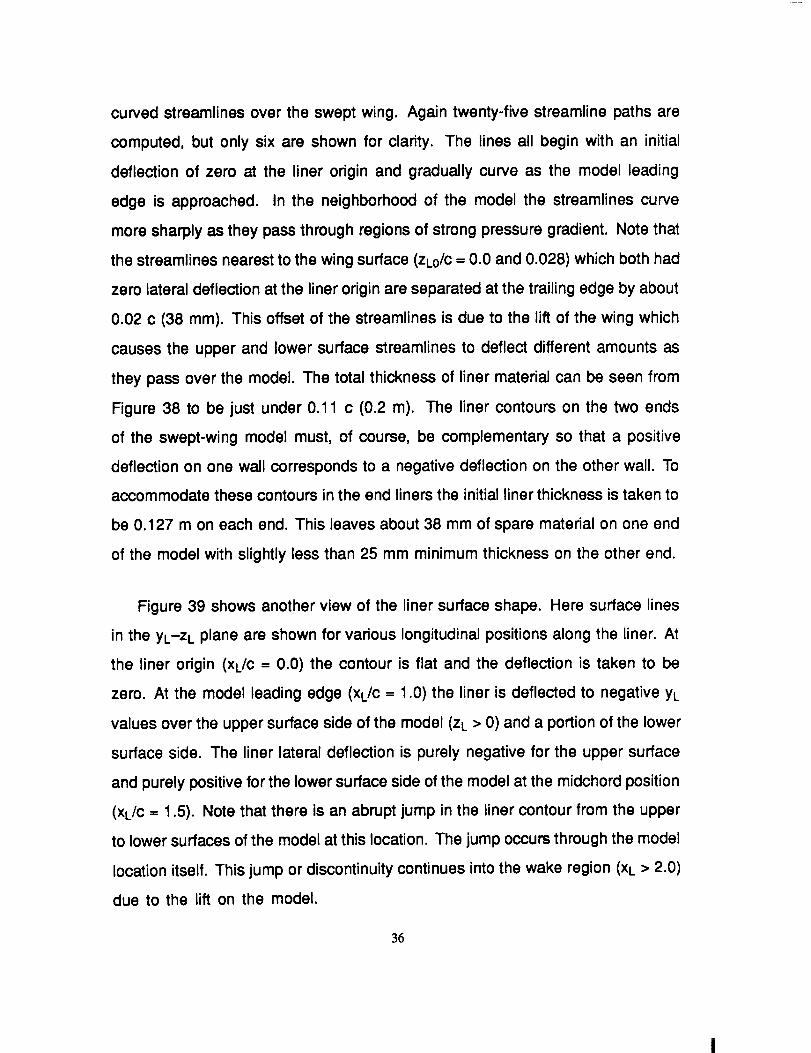
curved streamlines over the swept wing. Again twenty-five streamline paths are
computed, but only six are shown for clarity. The lines all begin with an initial
deflection of zero at the liner origin and gradually curve as the model leading
edge is approached. In the neighborhood of the model the streamlines curve
more sharply as they pass through regions of strong pressure gradient. Note that
the streamlines nearest to the wing surface (ZLo/C= 0.0 and 0.028) which both had
zero lateral deflection at the liner origin are separated at the trailing edge by about
0.02 c (38 ram). This offset of the streamlines is due to the lift of the wing which
causes the upper and lower surface streamlines to deflect different amounts as
they pass over the model. The total thickness of liner material can be seen from
Figure 38 to be just under 0.11 c (0.2 m). The liner contours on the two ends
of the swept-wing model must, of course, be complementary so that a positive
deflection on one wall corresponds to a negative deflection on the other wall. To
accommodate these contours in the end liners the initial liner thickness is taken to
be 0.127 m on each end. This leaves about 38 mm of spare material on one end
of the model with slightly less than 25 mm minimum thickness on the other end.
Figure 39 shows another view of the liner surface shape. Here surface lines
in the YL-ZL plane are shown for various longitudinal positions along the liner. At
the liner origin (XL/C = 0.0) the contour is flat and the deflection is taken to be
zero. At the model leading edge (XL/C = 1.0) the liner is deflected to negative YL
values over the upper surface side of the model (ZL > 0) and a portion of the lower
surface side. The liner lateral deflection is purely negative for the upper surface
and purely positive for the lower surface side of the model at the midchord position
(XL/C = 1.5). Note that there is an abrupt jump in the liner contour from the upper
to lower surfaces of the model at this location. The jump occurs through the model
location itself. This jump or discontinuity continues into the wake region (XL > 2.0)
due to the lift on the model.
36
A schematic view of the model and end liners installed in the UWT is shown
in Figure 40. The model is mounted with the wing chord plane vertical and
the contoured liners located on the floor and ceiling of the test section. The
contraction section of the tunnel is equipped with fairings which go from the
existing contraction contours to an initial liner depth of 0.127 m at the entrance of
the test section. The contraction fairings are each cut from a single large slab of
styrofoam material. The end liners are manufactured by laminating 51 mm x 152
mm x 1.22 m (2 in x 6 in x 4 ft) pieces of styrofoam material into blocks to form
the required liner thickness. The surface contour is then cut into each laminate
block using a heated-wire apparatus. This process results in a faceted shape to
the liners when all of the laminate blocks are assembled into the complete liner.
Figure 4 is a photograph of the composite liner during installation in the new UWT
test section. To complete the liner construction the styrofoam block surface is
sanded lightly to remove the facets and the surface is covered with a thin layer
of heat-shrink plastic film.
3?

5 EXPERIMENTAL RESULTS AND DISCUSSION
The experimental results are presented, analyzed, and compared with pre-
dictions from the linear stability theory in Chapter 5. Appendix B outlines the
hot-wire signal interpretation procedure. Measured wing pressure distributions
are given. The stationary-crossflow vortex pattern and the transition line are visu-
alized with sublimating-chemical and liquid-crystal surface coatings. Freestream
and boundary-layer velocity spectra are shown. Velocity profiles and contour
plots are given for the extensive hot-wire measurements taken across a single
stationary-crossfiow vortex track from x/c = 0.20 to 0.55 at Rc = 2.37 x 10⁶ and
= -4 °. These data include the mean-velocity, stationary crossflow-disturbance
velocity, and narrow band-pass travelling-wave velocity components in the stream-
wise direction. Theoretical stationary-crossflow disturbance-velocity data supplied
by Reed (Fuciarelli and Reed, 1992) are presented and transformed to various
coordinate systems for comparison with the experimental results. Theoretical
velocity-vector plots are shown overlaid on the experimental velocity-contours
plots. Observed stationary-crossflow vortex wavelengths and growth rates are
compared to theoretical predictions.
5.1 Freestream Flow Quality
The Unsteady Wind Tunnel is designed to operate as either an unsteady wind
tunnel or as a conventional low-turbulence tunnel. The tunnel is equipped with
an aluminum-honeycomb mesh and seven turbulence damping screens which
limits the freestream turbulence level to less than 0.04% Uoo in the low-turbulence
mode. For the present experiment the large-chord model and associated end
liners add disturbances which increase the background turbulence level somewhat
but it generally remains less than 0.09% Uoo which is still excellent flow quality
39
PREeEOiNG PhGE i:JLA_;,_ _'_OT FILMED ..-- .
for the crossflow experiments. A typical freestream velocity spectrum measured
with a hot wire for Rc = 2.66x10 s is shown in Figure 41. Most of the freestream
disturbance energy is concentrated at low frequencies. Above 10 Hz the energy
rolls off with increasing frequency out to about 100 Hz where the spectrum drops
below the electronic noise.
5.2 Pressure Distributions
Figures 42 and 43 show the measured wing-pressure distributions on the
upper surface, These data are measured for three different freestream velocities
and the three sets of data are almost indistinguishable. The pressure taps are
located in streamwise rows with one row near the top end of the model and the
other row near the bottom end. The data presented here are the swept-wing
pressure coefficients (Cp3) which differ from the airfoil pressure coefficients (Cp)
given in Chapter 4 by the square of the cosine of the sweep angle as
C = p-p°° = C cos2Ap3 ] 2_pU oo P
where p is the local surface pressure, Poo, p, and Uoo are the freestream pressure,
density, and velocity, respectively. For the top end of the model the measured
pressure distribution is in general agreement with the predicted curve, but the
theoretical pressure distribution slightly underestimates the measurements over
the whole model (Figure 42). The underestimate is largest in the region 0.05 < x/c
< 0.40. Examination of the top end liner contour indicates that the liner is slightly
thinner near the model leading edge than designed which probably accounts for
the under prediction of the pressure in this region. At the lower end of the model,
the experimental pressure distribution is well predicted back to about x/c = 0.25,
but the pressure minimum near x/c = 0.7 is under predicted (Figure 43). This
may occur because the test section floor is inclined to offset normal tunnel-wall
boundary layer growth on all four tunnel walls. Both the top and bottom rows of
4O
pressure taps are located within 5 to 15 cm of the liner surfaces which probably
exaggerates the influence of liner contour errors as compared to the impact felt
in the majority of the flow field. Since the measured pressure distributions differ
only slightly from the predicted distributions, it appears that in the central portion
of the test region a reasonable approximation of infinite swept-wing flow has been
established. The freestream and boundary-layer hot-wire measurements confirm
this.
5.3 Flow Visualizations
A naphthalene/trichlorotrifluoroethane spray is used to place a white subli-
mating coating over the black model surface. The naphthalene sublimes faster in
regions of high shear allowing the visualization of the stationary crossflow vortices
and clearly indicating the transition location. Figures 44-48 show naphthalene vi-
sualization photographs for c== -40 and chord Reynolds numbers ranging from
Rc = 1.93x10⁶ to Rc = 3.27x10⁶. The flow is from left to right on the Figures
with fractions of chord indicated by the markings at 10 percent chord intervals. In
each figure the naphthalene coating is absent over approximately the first 15% of
chord due to the high laminar shear stress in this region. From approximately x/c
= 0.15 back to the jagged transition line the stationary crossflow-vortex pattern is
clearly evident. The vortex spacing is determined by counting the number of light
and dark streak pairs over a 10 cm length. The wavelength is observed to remain
constant over the model at each test condition. This observation is in agreement
with the findings of Saric and Yeates (1985). In contrast to the results obtained
by Arnal and Juillen (1987) no vortex dropouts or other adjustments to the vortex
spacing are observed. The laminar region is terminated in each case at a jagged
transition line produced by overlapping turbulent wedges. Table 2 shows the av-
erage transition location and measured vortex spacing as a function of the chord
Reynolds number. The transition location is estimated from the photographs as
41
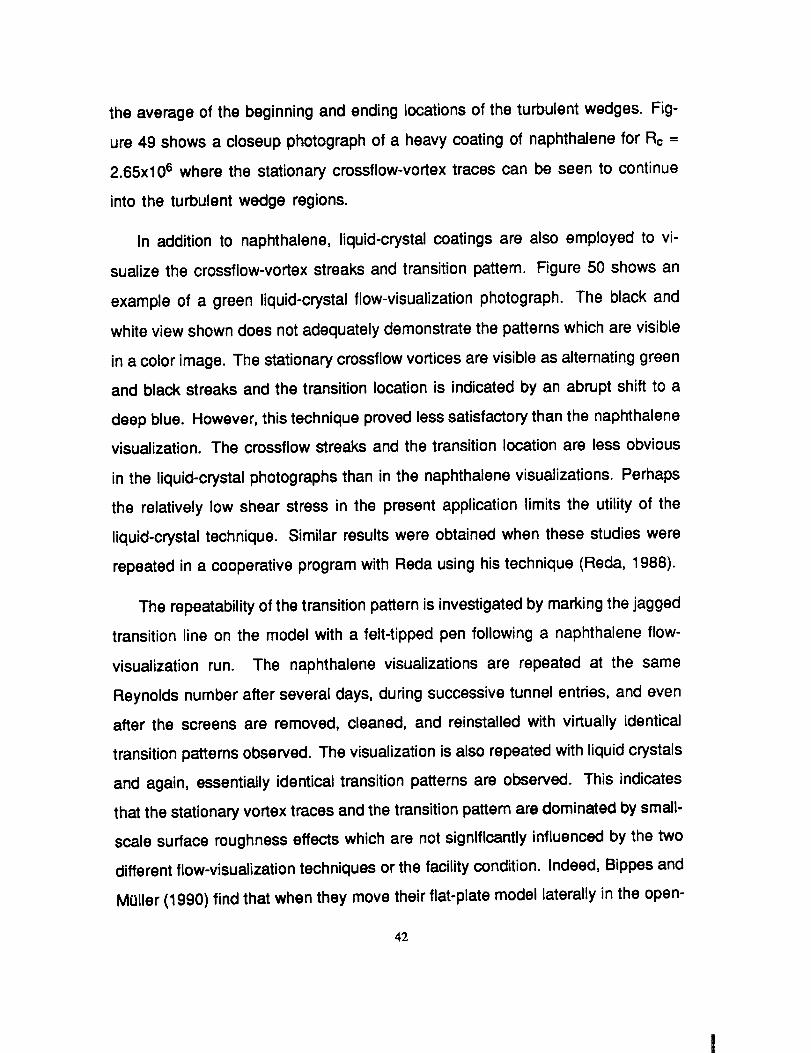
the average of the beginning and ending locations of the turbulent wedges. Fig-
ure 49 shows a closeup photograph of a heavy coating of naphthalene for Rc =
2.65x10⁶ where the stationary crossflow-vortex traces can be seen to continue
into the turbulent wedge regions.
In addition to naphthalene, liquid-crystal coatings are also employed to vi-
sualize the crossflow-vortex streaks and transition pattern. Figure 50 shows an
example of a green liquid-crystal flow-visualization photograph. The black and
white view shown does not adequately demonstrate the patterns which are visible
in a color image. The stationary crossflow vortices are visible as alternating green
and black streaks and the transition location is indicated by an abrupt shift to a
deep blue. However, this technique proved less satisfactory than the naphthalene
visualization. The crossflow streaks and the transition location are less obvious
in the liquid-crystal photographs than in the naphthalene visualizations. Perhaps
the relatively low shear stress in the present application limits the utility of the
liquid-crystal technique. Similar results were obtained when these studies were
repeated in a cooperative program with Reda using his technique (Reda, 1988).
The repeatability of the transition pattern is investigated by marking the jagged
transition line on the model with a felt-tipped pen following a naphthalene flow-
visualization run. The naphthalene visualizations are repeated at the same
Reynolds number after several days, during successive tunnel entries, and even
after the screens are removed, cleaned, and reinstalled with virtually identical
transition patterns observed. The visualization is also repeated with liquid crystals
and again, essentially identical transition patterns are observed. This indicates
that the stationary vortex traces and the transition pattern are dominated by small-
scale surface roughness effects which are not significantly influenced by the two
different flow-visualization techniques or the facility condition. Indeed, Bippes and
M011er(1990) find that when they move their flat-plate model laterally in the open-
42

jet test section the vortex-streak and transition patterns remain fixed and move
with the plate.
5.4 Transition Locations
Boundary-layer transition locations are determined by several methods in-
cluding interpretations of hot-film and hot-wire voltage signals and sublimating-
chemical flow visualizations. The transition locations are determined from the
flow-visualization photograph s by the abrupt shift in sublimation rate of the naph-
thalene coating due to turbulence-induced shear stress increases. The sharp
change from the streaked naphthalene pattern to black background thus marks
the transition location. The rms voltage responses of the hot-film gages are plot-
ted as functions of the Reynolds number. The point on the curve where the slope
increases abruptly with increasing Reynolds number is taken as the transition
point. For the boundary-layer hot-wire probes the onset of abrupt voltage spikes
in the time-dependent voltage signal is taken as the transition indicator. Thus,
all of these methods indicate the beginning of the transition process with the hot
wires and hot-film gages providing local transition measurements and the flow
visualization giving a global view of the transition pattern.
Figure 51 is a summary plot of transition measurements on the swept wing
versus chord Reynolds number for oe= -4 °. A transition band is indicated for the
naphthalene flow-visualization results. The beginning of the band indicates the
origin of the most forward turbulent wedge and the end of the band is the location
where the wedges merge. Points are shown for hot-wire transition measurements
at x/c = 0.4 and for hot-film transition measurements at several locations. Thus,
the naphthalene flow-visualization technique is calibrated. For chord Reynolds
numbers greater than 2.3x10 e the transition location is observed to be ahead of
43
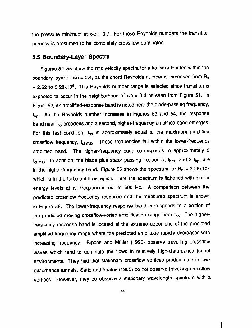
the pressure minimum at x/c = 0.7. For these Reynolds numbers the transition
process is presumed to be completely crossflow dominated.
5.5 Boundary-Layer Spectra
Figures 52-55 show the rms velocity spectra for a hot wire located within the
boundary layer at x/c = 0.4, as the chord Reynolds number is increased from Rc
= 2.62 to 3.28x10⁶. This Reynolds number range is selected since transition is
expected to occur in the neighborhood of x/c = 0.4 as seen from Figure 51. In
Figure 52, an amplified-response band is noted near the blade-passing frequency,
fbp. AS the Reynolds number increases in Figures 53 and 54, the response
band near fbp broadens and a second, higher-frequency amplified band emerges.
For this test condition, fbp is approximately equal to the maximum amplified
crossflow frequency, fcf max. These frequencies fall within the lower-frequency
amplified band. The higher-frequency band corresponds to approximately 2
fcf max. In addition, the blade plus stator passing frequency, fbps, and 2 fbp, are
in the higher-frequency band. Figure 55 shows the spectrum for Rc = 3.28x10⁶
which is in the turbulent flow region. Here the spectrum is flattened with similar
energy levels at all frequencies out to 500 Hz. A comparison between the
predicted crossflow frequency response and the measured spectrum is shown
in Figure 56. The lower-frequency response band corresponds to a portion of
the predicted moving crossflow-vortex amplification range near fbp. The higher-
frequency response band is located at the extreme upper end of the predicted
amplified-frequency range where the predicted amplitude rapidly decreases with
increasing frequency. Bippes and ML_ller (1990) observe travelling crossflow
waves which tend to dominate the flows in relatively high-disturbance tunnel
environments. They find that stationary crossfiow vortices predominate in low-
disturbance tunnels. Saric and Yeates (1985) do not observe travelling crossflow
vortices. However, they do observe a stationary wavelength spectrum with a
44

broad peak near the theoretically-predicted maximum-amplified wavelength and
an additional sharp peak at half the predicted wavelength. Reed (1988) is able
to explain this development as a parametric resonance between the primary
crossflow vortices which develop relatively far downstream and vortices of half
this wavelength which are slightly amplified in the thin upstream boundary layer.
5.6 Boundary-Layer Hot-Wire Surveys
5.6.1 Streamwise-Velocity Measurements
Constant-temperature hot-wire anemometers are used to make detailed mean
streamwise-velocity-profile measurements across a single stationary crossflow
vortex for a = --4 ° and Rc = 2.37x10 s. The measurements are made at intervals
of A(x/c) = 0.05 from x/c = 0.20 to x/c = 0.55 using two hot-wire elements. A
single hot-wire probe is located inside the boundary layer while a second single-
wire probe is located in the freestream. Both wires are oriented parallel to the
model surface and perpendicular to the freestream velocity vector. The ratio of the
velocity indications from the two anemometers yields the streamwise boundary-
layer velocity ratio. The hot-wire calibration and data reduction procedure is given
in Appendix B. The experimental error analysis is given in Appendix C. Figure
20 shows that the stationary crossflow vortices become unstable at x/c = 0.05
while Figure 51 shows that the average transition line lies at approximately x/c
= 0.58. Thus, the measurement locations cover a large portion of the unstable
crossflow region from slightly downstream of the first neutral point to just ahead
of the transition location.
A high-shear vortex track (i.e., dark streak) on the model is marked with a
soft felt-tipped pen following a sublimating chemical flow-visualization study. The
beginning point of the track is arbitrarily chosen to be the midspan location for
x/c = 0.20. For most locations the measurements are made at seven spanwise
45
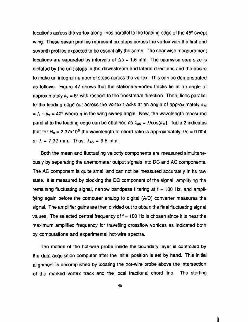
locations across the vortex along lines parallel to the leading edge of the 45 ° swept
wing. These seven profiles represent six steps across the vortex with the first and
seventh profiles expected to be essentially the same. The spanwise measurement
locations are separated by intervals of/ks = 1.6 mm. The spanwise step size is
dictated by the unit steps in the downstream and lateral directions and the desire
to make an integral number of steps across the vortex. This can be demonstrated
as follows. Figure 47 shows that the stationary-vortex tracks lie at an angle of
approximately 0v = 50 with respect to the freestream direction. Then, lines parallel
to the leading edge cut across the vortex tracks at an angle of approximately ea
= A - 0v = 40 ° where A is the wing sweep angle. Now, the wavelength measured
parallel to the leading edge can be obtained as A45 = A/cos(SM). Table 2 indicates
that for Rc = 2.37x10 e the wavelength to chord ratio is approximately A/c = 0.004
or A = 7.32 mm. Thus, A4,5 = 9.5 ram.
Both the mean and fluctuating velocity components are measured simultane-
ously by separating the anemometer output signals into DC and AC components.
The AC component is quite small and can not be measured accurately in its raw
state. It is measured by blocking the DC component of the signal, amplifying the
remaining fluctuating signal, narrow bandpass filtering at f = 100 Hz, and ampli-
fying again before the computer analog to digital (ND) converter measures the
signal. The amplifier gains are then divided out to obtain the final fluctuating signal
values. The selected central frequency of f = 100 Hz is chosen since it is near the
maximum amplified frequency for travelling crossflow vortices as indicated both
by computations and experimental hot-wire spectra.
The motion of the hot-wire probe inside the boundary layer is controlled by
the data-acquisition computer after the initial position is set by hand. This initial
alignment is accomplished by locating the hot-wire probe above the intersection
of the marked vortex track and the local fractional chord line. The starting
46

point for each boundary-layer survey station is set in this fashion. During the
data-acquisition procedure, the experimenter has to actively observe the hot-
wire AC signals on an oscilloscope, adjust the amplifier gain settings to assure
maximum signal strength with overranging the instruments, and stop the traverse
mechanism before the probe collides with the model surface. The data-acquisition
computer measures the anemometer voltages and moves to the next point only
after acceptance of the data by the experimenter.
The velocity data are presented in Figures 57-120 in two forms m as velocity
profiles at several spanwise stations across the crossflow vortex and as veloc-
ity contours over the 45 ° spanwise measurement cuts. Figures 57-64 show the
actual velocity ratio values obtained from the hot-wire data reduction procedure
outlined in Appendix B. The height above the wing surface is determined by ex-
trapolating the velocity data to a zero value at the surface for each profile. The
presence of the stationary crossflow vortex is indicated in Figures 65-72 by sub-
tracting the average value of the streamwise velocity from the local profile values.
The resultant disturbance velocity profiles show the excess or deficit of velocity
produced by the stationary vortex. An alternate representation of the stationary
crossflow-vortex disturbance intensity is given in Figures 73-80 where reference
computed velocity profiles are subtracted from the local velocity measurements.
In both of these representations, the velocity difference is made nondimensional
by dividing by the local boundary-layer edge velocity magnitude. Thus, the plots
represent local disturbance intensity values, but, since the boundary-layer edge
velocity increases slightly from x/c -- 0.20 to 0.55 the velocity ratios are scaled
down by a small amount as x/c increases. The root-mean-square velocity pro-
files for f = 100 Hz travelling waves are given in Figures 81-88. The velocity
values are again nondimensionalized by the local boundary-layer edge velocity.
Contour plots of the mean streamwise velocity across the vortex are shown in
4?
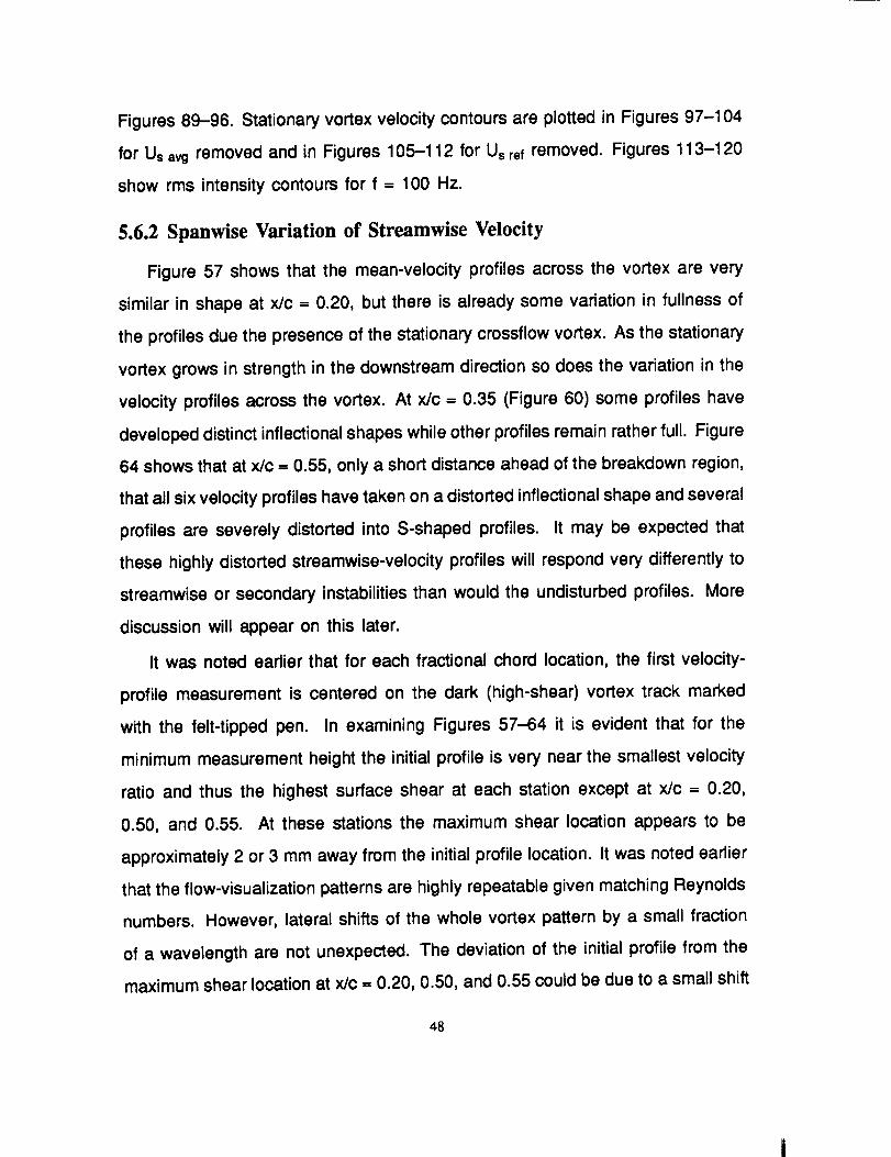
Figures 89-96. Stationary vortex velocity contours are plotted in Figures 97-104
for Us avg removed and in Figures 105-112 for Us ref removed. Figures 113-120
show rms intensity contours for f = 100 Hz.
5.6.2 Spanwise Variation of StreamwJse Velocity
Figure 57 shows that the mean-velocity profiles across the vortex are very
similar in shape at x/c = 0.20, but there is already some variation in fullness of
the profiles due the presence of the stationary crossflow vortex. As the stationary
vortex grows in strength in the downstream direction so does the variation in the
velocity profiles across the vortex. At x/c = 0.35 (Figure 60) some profiles have
developed distinct inflectional shapes while other profiles remain rather full. Figure
64 shows that at x/c = 0.55, only a short distance ahead of the breakdown region,
that all six velocity profiles have taken on a distorted inflectional shape and several
profiles are severely distorted into S-shaped profiles. It may be expected that
these highly distorted streamwise-velocity profiles will respond very differently to
streamwise or secondary instabilities than would the undisturbed profiles. More
discussion will appear on this later.
It was noted earlier that for each fractional chord location, the first velocity-
profile measurement is centered on the dark (high-shear) vortex track marked
with the felt-tipped pen. In examining Figures 57-64 it is evident that for the
minimum measurement height the initial profile is very near the smallest velocity
ratio and thus the highest surface shear at each station except at x/c = 0.20,
0.50, and 0.55. At these stations the maximum shear location appears to be
approximately 2 or 3 mm away from the initial profile location. It was noted earlier
that the flow-visualization patterns are highly repeatable given matching Reynolds
numbers. However, lateral shifts of the whole vortex pattern by a small fraction
of a wavelength are not unexpected. The deviation of the initial profile from the
maximum shear location at x/c = 0.20, 0.50, and 0.55 could be due to a small shift
48

in the vortex pattern or to a small lateral misalignment (~ 2 to 3 mm) of the traverse
rig at the beginning of the measurements. The influence of this misalignment at
the beginning of the measurement region will be evident in results to follow.
5.6.3 Disturbance Profiles
Figures 65-72 show the stationary crossflow-disturbance velocity profiles de-
termined by subtracting the average streamwise-velocity ratio at a given height
from the measured velocity ratio at each location. The abscissa scale is chosen
to keep the local velocity scales essentially the same for each chordwise sta-
tion. As noted previously, the local boundary-layer edge velocity, which is used
as a reference value, increases slightly from x/c = 0.20 to x/c = 0.55 so that
the disturbance velocity ratios are scaled down slightly with this nondimension-
alization as x/c is increased. For the crossflow instability, the disturbance vortex
axes are nearly streamwise and the primary disturbance-vortex components in a
streamwise coordinate system are the v- and w-velocity components. The per-
turbation in the streamwise direction (u-component) is a secondary effect due to
the convection arising from the v- and w-velocity components. However, the
streamwise component (U-component) of the boundary-layer velocity has a large
gradient in the direction perpendicular to the wing surface (dU/dy) which when
combined with small convective v- and w-velocity components produces a large
secondary streamwise-velocity perturbation. This streamwise-velocity perturba-
tion is the one shown in Figures 65-72 and later in Figures 73-80. It is to be
expected that over a single vortex wavelength, these perturbation velocity profiles
will exhibit either excesses or deficits from the mean, depending on the lateral lo-
cation in the streamwise vortex. Over that portion of the vortex where the v- and
w-velocity components convect the high-momentum flow from the outer portion of
the boundary layer toward the surface the local profile should have an excess (or
bulging) shape. On the other hand, when the vortex-velocity components convect
49
low-momentum flow away from the surface the local profile is expected to have
a deficit shape.
Note that in Figures 65 and 67 only five velocity profiles are measured.
Nonetheless, it is apparent in Figure 65 that some of the local disturbance
profiles show excess velocities while others show deficit velocities as expected.
However, the profiles in Figure 65 have two unexpected features. First, the
disturbance profiles do not approach zero for large values of the height, y, above
the wing surface. This is due to temperature drift effects in the Unsteady Wind
Tunnel. The UWT has no temperature control; the test temperature is governed
by the ambient temperature in the wind-tunnel building (which is cooled by an
electrical air-conditioning unit) and, more importantly, by the power input to the
wind-tunnel fan. To eliminate this effect for the other measurement stations
the tunnel was run in a preheat mode for 30 to 45 minutes before acquiring
boundary-layer disturbance data. This preheat time is used each day to verify
instrumentation connections, filter settings, and so forth. The second anomalous
aspect of the profiles in Figure 65 is the bulge in excess and deficit velocities
below about y = 0.5 mm. These bulges are unexpected and are almost as large
as the maximum disturbance intensities found for y _ 1.2 ram. The presence
of these velocity perturbations is traced to residue left behind by cleaning the
model with alcohol and supposedly lint-free cloths. This contamination had not
been noted earlier during the preliminary velocity-profile measurements probably
because single velocity-profile measurements were generally made following a
flow-visualization study in which the model surface was effectively cleaned by the
tdchlorotrifluoroethane solvent used with the naphthalene. The model cleaning
procedure was modified to a two-step procedure -- cleaning first with alcohol
and then with distilled water. A single velocity-profile measurement at x/c = 0.20
confirmed that the residue problem was solved, but the complete set of velocity
5O
profiles at x/c = 0.20 were not measured again due to lack of sufficient time. The
data at all subsequent measurement stations are taken following the two-step
model cleaning process and no further contamination problems are encountered.
Examination of Figures 65-72 shows that the maximum disturbance intensity
of the stationary crossflow vortex grows progressively from x/c = 0.20 back to x/c
= 0.55. At x/c = 0.20 the profiles show either excess or deficit velocities only. But
by x/c = 0.35 some of the disturbance profiles have taken on definite crossover
shapes. These crossover profiles have both excess and deficit velocity regions.
At the last measurement station (x/c = 0.55) the maximum disturbance intensity
exceeds 20% of the edge velocity and all of the profiles have taken on highly
distorted shapes. The nature and significance of these crossover profiles will
be discussed further in the following section where the disturbance velocities are
displayed as contour plots.
Figures 73-80 show stationary crossflow-disturbance profiles obtained by a
different procedure. Here local theoretical velocities are subtracted from the
measured profiles to yield the local disturbance vortex intensities. Note that the
angle of attack for the reference case is taken as _ = -5 ° rather than the actual
angle of attack o_ = -4 °. This adjustment in the theoretical angle of attack is
required because the theoretical profiles for a = -40 are obviously fuller than the
experimentally measured profiles. The reason for this discrepancy is uncertain,
but it may arise from a slight flow angularity in the UWT test section or a minor
misalignment of the model mounting bearing.
The stationary crossflow profiles in Figures 73-80 agree in general trends with
those shown in Figures 65-72. In both cases, the maximum disturbance intensity
grows progressively with increasing x/c, definite crossover profiles develop by
xJc = 0.35, and at x/c = 0.55 all profiles are highly distorted. However, there
are some slight differences between removing the average velocity profile and
5!

the theoretical velocity profile from the measured data. These differences arise
because the averaged profiles from the experiment include flow history effects
produced by the presence of the stationary crossflow vortices within the boundary
layer while the theoretical profiles completely neglect this effect. The most notable
of the differences in the two sets of profiles is observed by comparing Figures 65
and 73 for x/c = 0.20. In Figure 73, the influence of the surface contamination
discussed earlier produces velocity deficits in all profiles for y < 0.5 mm. In
Figure 65, this deficit effect is included in the averaged profile and as a result
the disturbance profiles are not biased toward a deficit condition. Of course, this
deficit effect is an experimental error which would have been removed completely
by retaking the data at x/c = 0.20 if time had allowed. Other notable, and
experimentally more significant, differences are observed for x/c > 0.45 where
flow history effects become more pronounced. This effect will be shown more
clearly in the disturbance-velocity contour plots which are shown later.
Root-mean-square velocity profiles for travelling waves are shown in Figures
81-88. As mentioned previously, these data are measured simultaneously with
the mean velocity by splitting the hot-wire anemometer signal into mean and
fluctuating components. The fluctuating component is amplified, narrow bandpass
filtered, and amplified again before recording with the UWT A/D converter system.
The selected central frequency for the narrow bandpass filter is f = 100 Hz which is
near the frequency of maximum amplification according to both experimental and
theoretical considerations. Again, these data are plotted with an abscissa scale
which is essentially unchanged over the range of measurement locations. This
allows for easy visual examination of the disturbance amplification with increasing
x/c. For travelling crossflow waves rms averaged profiles of the streamwise
velocity are expected to yield profiles with a single maximum and, of course,
only positive values. Furthermore, in the absence of nonlinear distortions due to
52
the stationary crossflow vortices or the presence of some other travelling waves
in the same frequency range the rms velocity profiles are expected to be identical
at each spanwise location.
For the first two measurement stations (x/c = 0.20 and 0.25, Figures 81 and 82)
the disturbance intensities are quite small and the velocity profiles have essentially
the same shape at all spanwise locations across the stationary crossflow vortex.
Here the rms streamwise-velocity profiles have a single lobe (or maximum) as
expected for travelling crossflow vortices. By x/c = 0.30 the shapes of the
travelling-wave velocity profiles have begun to distort, but the profiles continue
to have single-lobed shapes. This distortion of the profile shape may arise
from the development of other travelling-wave disturbance modes of the same
frequency, but different direction of travel, or the nonlinear distortion of travelling-
crossflow waves by the strong stationary crossflow-vortex layer. For x/c > 0.40
(Figures 85-88) definite double-lobed travelling-wave disturbance velocity profiles
are apparent at some spanwise locations across the stationary crossflow vortex.
Between x/c = 0.40 and 0.50 the travelling waves grow considerably in strength.
However, from x/c = 0.50 to 0.55 the largest amplitudes decrease by greater than
a factor of two. Note that even at their maximum intensity, the travelling waves
are quite small as compared to the strength of the stationary crossflow vortex (i.e.,
only 3.5% as large). Thus, it appears that the travelling waves which initially have
very low amplitude, grow and distort considerably for 0.40 < x/c < 0.50, and then
decay for x/c > 0.50. The nature of the distortion of the travelling waves due to
the stationary crossflow vortices will be more apparent when viewed as contour
plots in the following section.
5.6.4 Streamwise-Velocity Contour Plots
Contour plots of the mean velocity, stationary crossflow-disturbance intensi-
ties, and the travelling-wave disturbances are given in Figures 89-120. These
53
plots show the various experimentally-determined quantities plotted on a grid
which is 4 mm deep in the y (or surface normal) coordinate and stretches 9.5
mm along a 45 ° swept line parallel to the wing leading edge. As mentioned previ-
ously, the spanwise coordinate cuts across the stationary crossflow-vortex tracks
at an approximately 40 ° angle and the stationary-vortex wavelength along a line
parallel to the leading edge is ,_ -- 9.5 mm. The abscissa is taken as z_ =
-(Zm-Zmo)/_4s and is a local coordinate with z k = 0 on the marked stationary-
vortex track and z_ > 0 the direction of spanwise motion of the hot-wire probe.
With this coordinate selection, the abscissa actually runs in the direction opposite
to the model spanwise coordinate, Zrn. The plots show the situation an observer
would see when looking upstream from the hot-wire probe location. These data
are plotted for 0.20 < x/c < 0.55 in increments of z3(x/c) -- 0.05. For x/c -- 0.20 and
0.30, the data are not measured across the full crossflow-vortex wavelength. But,
for the other stations, these data are shown for a full stationary crossflow-vortex
wavelength. For each boundary-layer station all velocities are made nondimen-
sional by dividing by the local streamwise boundary-layer edge velocity. Since the
edge velocity increases by about 10% from x/c = 0.20 to 0.55 the actual velocities
are scaled down by this factor.
89-96 show the mean streamwise boundary-layer velocity ratio, Z_-,Figures
in the tunnel coordinate frame, in the absence of stationary crossflow-disturbance
vortices, the velocity contours are expected to be flat and parallel to the wing
surface. Figure 89 shows that the mean-velocity contours at x/c = 0.20 are,
indeed, nearly flat and parallel to the wing surface. But, some influence of
the stationary crossflow vortex is already present at this forward location with
the contour levels somewhat wavy and inclined slightly toward the surface for
increasing values of z_. The waviness of the contours increases with x/c until the
contours obviously bulge upward at approximately the middle of the wavelength
54
for x/c = 0.35 (Figure 92). This upward bulge of the contours corresponds to
low-momentum fluid being swept upward from the wing surface by the stationary
crossflow vortex. The bulge continues to grow as x/c increases until the contours
actually begin to roll over like a breaking wave for x/c > 0.50 (Figures 95 and 96).
This mean-velocity contour pattern is consistent with expectations for
boundary-layer flow with imbedded stationary crossflow vortices which will be illus-
trated more fully in the next section. The flow-visualization photographs (Figures
44-48) show that the crossflow-vortex axes are aligned almost parallel to the
freestream velocity vector. The instability produces a layer of counter-rotating
disturbance vortices which combine with the mean boundary-layer crossflow to
yield a layer of crossflow vortices all with the same rotational direction (co-rotating
pattern). The flow field is illustrated more fully later in Section 5.7.1. This pattern
develops because the flow is most unstable to the crossflow instability at some
small angle to the pure crossflow direction (Dagenhart, 1981). The mean-velocity
profile in the most unstable crossflow direction has a crossover shape with flow
streaming in the crossflow direction near the wing surface, but in the opposite
direction further out from the surface (Gregory, Stuart, and Walker, 1955). When
this crossover velocity profile is combined with the counter-rotating disturbance
vortices, it reinforces the strength of one of the pair of vortices while cancelling
the other. This produces the observed velocity field with flow streaming in the
crossflow direction near the wing (z _-direction) while the flow in the outer part
of the boundary layer flows in the opposite direction. Hence, the breaking-wave
pattern seen in Figures 95 and 96.
As previously noted, the initial velocity profile at each measurement station
is intended to be on the line of maximum shear as determined by the flow-
visualization study. But, since the measurements are made over many days
of wind-tunnel testing, it is not unexpected that small shifts (,._ 2 to 3 mm) in
55

the location of the stationary vortex pattern might occur. Such shifts in the vortex
pattern can be deduced from the mean streamwise velocity-contour plots (Figures
89-96). The maximum surface shear stress location is determined qualitatively
by observing the crowding of streamwise-velocity contours near the wing surface.
Figures 95 and 96 show that the maximum shear stress point appears to have
shifted by 1.5 to 3 mm in the z k-direction. This shift will be even more obvious
in the stationary-vortex velocity field which follows.
Stationary crossflow-vortex velocity contours are plotted in Figures 97-104 and
85-92. The first set of contours corresponds to disturbance velocities determined
by subtracting the theoretical mean-velocity values from the measured velocities.
The second set of disturbance velocity contours are computed by removing the
averaged mean-velocity profile from the local measured velocities. In each case
the disturbance velocity values are nondimensionalized by the local boundary-
layer edge velocity which increases slightly from x/c = 0.20 to 0.55. The range of
contour levels up to i0.20 Us e are used for all measurement locations for easy
data comparisons. The two sets of contours agree in general shape and levels of
the velocity contours. Some relatively small differences can be noted for x/c = 0.50
and 0.55 where the averaged mean-velocity profile is distorted by the presence of
the stationary crossflow vortex, but the theoretical profiles ignore this effect. Thus,
the following discussion of the evolution of the stationary crossflow-disturbance
velocity contours applies equally well to either set of Figures.
The expected stationary crossflow-disturbance velocity pattern has excess
velocities at the extremes of the plotting field (z_ = 0 and 1) and deficit velocities
near the middle of the field (z_ = 0.5). This is because the initial velocity profile (z_
= 0) is measured at the supposed maximum shear point which should correspond
to high-momentum fluid being swept toward the wing surface. This situation
should, of course, recur one full wavelength away (z_ = 1). Velocity deficits
56

should occur where the stationary crossflow vortex sweeps flow away from the
surface (z_ = 0.5). Figures 97 and 105 show that at x/c = 0.20 the presence
of the stationary crossflow vortices is already detectable with velocity variations
exceeding 4-0.02 Us e. The expected velocity pattern is not evident for x/c = 0.20
or 0.25 (Figures 97-98 and 105-106), but it emerges for x/c = 0.30 (Figures 99
and 107). The periodicity of the velocity perturbations is clearly evident for 0.35
< x/c < 0.55 (Figures 100-104 and 108-112). For x/c = 0.35, 0.40, and 0.45 the
excess velocities occur at the ends of the measurement zone and the deficits in
the middle as expected. For x/c = 0.50 and 0.55 the peak excess velocities are
shifted in the +z),-direction by approximately 2 mm. This seems to correspond
to and is consistent with the observed shift in the maximum shear stress location
as discussed previously.
The stationary crossflow-disturbance velocities are quite small at the beginning
of the measurement region (x/c -- 0.20). The disturbances grow progressively
larger with increasing x/c back to x/c = 0.50 until they exceed +0.20 Us o. From
x/c = 0.50 to 0.55 the deficit velocities continue to increase in intensity, but
the velocity excesses drop sharply. This decrease in excess velocity intensity
seems surprising since the linear stability analysis presented earlier (see Figure
20) shows that the stationary crossflow-disturbance vortices should be amplified
all the way back to the pressure minimum at x/c = 0.71. For the present case
(Rc = 2.37x10⁶) the average transition line is determined by the flow-visualization
studies to be at approximately x/c = 0.58 (see Figure 51 and Table 2). It may be
that between x/c = 0.50 and 0.55 energy is being extracted from the stationary
crossflow vortices and pumped into some other disturbance mode such as the
secondary instability mode.
Figures 113-120 show contour plots of the temporal rms velocities of travelling
waves with f = 100 Hz for x/c = 0.20 to 0.55. These velocities are again made
5?

nondimensional by dividing by the local boundary-layer edge velocity. It was
indicated earlier that f -- 100 Hz corresponds to a peak in both the measured
and theoretical boundary-layer velocity spectra. The rms values measured are
quite small with the maximum values being approximately 0.7% Us e. The same
contour levels are used for all the plots so that the disturbance levels can be readily
compared. In the absence of complicating factors such as nonlinear interaction
with stationary crossflow vortices or the presence of other travelling waves in the
same frequency range, the rms velocity contours are expected to be flat and
parallel to the wing surface.
The travelling-wave intensities are essentially zero for 0.20 < x/c < 0.30
(Figures 113-115). For x/c = 0.35 and 0.40 the peak disturbance amplitudes range
from about 0.07% to 0.1% Use (Figures 116 and 117) and the contour lines are
very roughly parallel to the wing surface, as anticipated for undistorted travelling-
crossflow waves. The disturbance velocity profiles shown earlier in Figures 83 and
84 for these locations also have the expected single-lobed shapes. By x/c = 0.40
(Figure 118) definite closed-contour shapes have developed. This corresponds
to the development of double-lobed disturbance profiles (Figure 86). Between
x/c = 0.45 and 0.50 the travelling wave disturbance strength grows dramatically
with the maximum rms intensity reaching 0.7% Us g. The disturbance intensity also
departs strongly from the ideal of equal distribution along the span to peak sharply
near the center of the vortex wavelength. Perhaps significantly, Figure 63 shows
that near the middle of the measurement zone that the streamwise-velocity profile
takes on a distinctly distorted S-shape. From x/c = 0.50 to 0.55 the strength of the
travelling waves drops precipitously (Figure 120) and the maximum contour levels
shift location. The sharp drop in travelling-wave intensity occum even though
the streamwise mean-velocity profiles continue to develop ever more distorted
S-shaped profiles (Figure 64). This is in the same region where the stationary
58
crossflow vortices are observed to decrease in strength although the decrease
is not so pronounced in the stationary vortex case. As mentioned previously,
in the region from x/c = 0.50 to 0.55 energy may be transferred to other high-
frequency modes which lead to laminar flow breakdown in the neighborhood of
x/c = 0.58. The nonuniform nature of the rms disturbances along the span seems
to indicate that the travelling waves detected may not be travelling crossflow
vortices, but some other travelling waves in the same frequency range (possibly
Tollmien-Schlichting waves generated at the locations of the S-shaped mean-
velocity profiles).
5.7 Experimental/Theoretical Comparisons
In the previous sections, experimental velocity profiles and contours are shown
along a single vortex track on the 45 ° swept wing for c_= -4 ° at Rc = 2.37x10⁶.
Both mean and disturbance velocities extracted from the mean data are given.
In this section, those experimental data and other results obtained from them
are compared to linear stability theory predictions supplied by Reed using her
theoretical code (Fuciarelli and Reed, 1992). This theoretical code is used
because it gives both growth rates and disturbance eigenfunction profiles whereas
the MARIA (Dagenhart, 1981) and SALLY (Srokowski and Orszag, 1977) codes
employed earlier give only growth rates. The mean-velocity profiles supplied to
Reed and shown below were computed using the method of Kaups and Cebeci
(1977). As mentioned previously, theoretical data for (x = -5 ° are used for this
comparison because these data seem to yield a better match to the experimental
data which are measured at a nominal angle of attack of Q = -40. A small flow
angularity in the UWT test section or a slight misalignment of the model could
account for this difference.
59
5.7.1 Theoretical Disturbance Profiles
Figures 121 and 122 show the mean-velocity profiles at the experimental mea-
surement stations computed using the method of Kaups and Cebeci (1977). The
velocity components are given in a model-oriented coordinate system (xm,Ym,Zm)
with Xm perpendicular to the wing leading edge, Ym normal to the wing-chord
plane, and zm parallel to the wing leading edge (See Appendix A). Note that the
spanwise velocities, Wm/Ut • are taken to be negative. This occurs because Reed
chooses to use a left-handed coordinate system so that the crossflow wave num-
bers are both positive. The experimental data presented in the previous sections
are shown from the perspective of the hot-wire measurement probe looking up-
stream. This constitutes essentially a conversion of the experimental coordinate
frame into a left-handed system. Thus, the experimental and theoretical data can
be compared directly. Stationary crossflow-instability eigenfunctions are shown in
Figures 123-125 for each of the coordinate directions. The computations are for
a fixed wavelength of A = 7 mm which essentially matches the experimentally ob-
served wavelength of Mc = 0.004 or A = 7.3 mm. The profiles are scaled to match
the experimentally-determined maximum streamwise-disturbance amplitudes at
each measurement station. This is permissible, of course, since linear stability
theory predicts the actual disturbance intensity only to within a rnultiplicative con-
stant. The phase relationships between the velocity components are not shown
in the figures, although they are critically important to the determination of the
spatial velocity field of the instability waves. Note also that in the model-oriented
coordinate frame, the disturbance velocities in the chordwise direction, urn, and
the spanwise direction, win, are of the same order while the normal-velocity com-
ponent, Vm, is an order of magnitude smaller.
For comparison with the experimental data the velocity profiles given in Figures
121-125 must be rotated about the y-axis to two other coordinate reference
6O
frames. One of these frames, the streamwise frame, (Xs,Ys,Zs), is oriented with
Xs parallel to the freestream-velocity vector and Ys perpendicular to the wing-
chord plane while in the other frame, the wave-oriented frame, (xw,Yw,Zw), Xw is
along the vortex axis and Zw is parallel to the wavenumber vector. Of course,
Ym, Ys, and Yw are all parallel. The experimental measurements are made in the
streamwise coordinate frame, (Us,Ys,Zs). The theoretical vortex flow pattern in the
wave-oriented frame, (xw,Yw,Z,), will be superposed onto the experimental data
plots. The relationships between these coordinate frames are given in Appendix A.
The mean flow velocity components in the (Xs,Ys,Zs) frame are shown in Fig-
ures 126 and 127. In this coordinate frame (See Appendix A), the cross-stream
mean velocities, Ws, are considerably smaller than the streamwise velocities,
Us. Likewise the cross-stream disturbance velocities, Ws, are much smaller than
the streamwise-disturbance velocities, Us (See Figures 128 and 129). Figures
130-133 show the mean- and disturbance-velocity components in the wave-
oriented coordinate frame. Here both the mean and disturbance velocity com-
ponents in the Zw direction are an order of magnitude smaller than the respective
velocities components along the vortex axis. In this frame, Ww is the same order of
magnitude as Vw = Vm. Thus, in both the wave-oriented and streamwise-oriented
coordinate frames the velocities along the x-axes are much larger than the velocity
components in the other two directions.
The nature of the disturbance-vortex flow is illustrated in Figures 134-136.
A vector plot of (vw,Ww), across a single vortex wavelength is shown in Figure
134 in the wave-oriented coordinate frame. The vectors are the projections of
the disturbance-velocity vectors onto the yw-Zw plane. The disturbance is seen to
consist of a pair of counter-rotating vortices within a single wavelength. The vortex
cells are skewed so that a central counterclockwise-rotating vortex is bordered
on each side by a portion of the alternate clockwise-rotating vortices. In Figure
6]
135 the mean plus disturbance velocity vectors, (Vw,Ww+Ww) are plotted over a
single wavelength. Here the mean normal velocity, Vw, which is quite small has
been neglected. Note that the mean velocity, Ww (See Figure 131) completely
dominates the vector field masking the presence of any disturbance vorticity. The
presence of the disturbance vorticity can be illustrated by arbitrarily scaling the Vw
velocities by a factor of 100. This is shown in Figure 136 where it is apparent that
the mean plus disturbance flows combine to produce a single counterclockwise-
rotating vortex per wavelength. That is, the total flow consisting of disturbances
superposed on a base flow contains a layer of co-rotating vortices.
5.7.2 Disturbance Profile Comparisons
Experimental stationary crossflow-disturbance profiles (from Us - Us avg) are
compared with the linear-theory eigenfunction magnitudes in Figures 137-144. In
each case the streamwise-disturbance velocity profiles are shown. Similar results
are found using the experimental profiles determined from Us - Us ref (Figures
73--80) but these are not shown. The experimental profiles are determined
by taking the spatial rms of the individual profiles (Figures 65--72) across the
stationary vortex. This procedure is the spatial analog for a stationary wave of
taking the temporal rms of a travelling wave. All of the profiles are plotted on the
same abscissa scale (made nondimensional by reference to the local boundary-
layer edge velocity) for easy visual comparison of the disturbance growth with
distance along the wing. The theoretical eigenfunctions which have only a single
lobe (See Figure 128) are scaled to match the peak experimental amplitude at
each measurement location.
At x/c = 0.20 (Figure 137) the theoretical and experimental profiles are of
similar shape in the region of the maximum amplitude near y = 1 ram, but
the two curves diverge in the near-surface region and in the outer flow. As
mentioned previously the measured profiles at this location are thought to contain
62

experimental errors which are rectified for the remaining measurements. The
near-surface results are affected by a lint-contaminated surface and the outer
flow measurements are affected by tunnel-temperature drift. For x/c = 0.25, 0.30,
0.35, and 0.40 (Figures 138-141) the experimental and theoretical profiles are of
similar single-lobed shapes. However, the point of maximum disturbance intensity
is slightly higher in the boundary layer for the theoretical eigenfunctions than for
the experimental profiles.
For x/c = 0.45 and beyond (Figures 142-144) the experimental profiles take
on double-lobed shapes which contrast with the single-lobed theoretical eigen-
functions. The point of maximum disturbance strength for the theoretical profiles
lies between the two maxima of the experimental profiles. Recall from the earlier
discussion that for x/c = 0.45 and beyond, the local experimental disturbance pro-
files take on crossover shapes which are not anticipated from the linear theory.
This is evident in the local profile plots of Figures 70-72 and 78-80 as well as
the disturbance velocity-contour plots of Figures 102-104 and 110-112. Figures
94-96 show that the mean streamwise-velocity contours for 0.60 < Us/Us • < 0.90
rise sharply from the model surface and begin to roll over. That this is due to the
presence of the stationary crossflow vortex will become evident in the next section.
Thus, there is general agreement between the shapes of the experimental
disturbance velocity profiles and the theoretical eigenfunctions up to about x/c =
0.40 where the rms intensity of the stationary vortices is about 7% of Us. But for
x/c = 0.45 onward, the presence of the stationary crossflow vortices distorts the
experimental disturbance profiles into double-lobed shapes not predicted by the
linear theory. This does not necessarily mean that nonlinear effects are present,
even though the stationary disturbance intensities (+20% Us at xJc = 0.50) are
well beyond the small perturbation limits assumed in the linear theory. In fact, the
observed effects may simply be due to flow history. That is, the strong stationary
63
crossflow vortices continually lift low-speed fluid up from the surface and push
high-speed fluid downward so that the flow wraps around the vortex axis. More
will be shown on this point in the next section.
5.7.3 Comparison of Experimental Streamwise Velocity-ContourPlots and Theoretical Vector Plots
Figures 145-152 show theoretical velocity vectors superposed on the experi-
mental streamwise velocity-contour plots. Theoretical velocity vectors are super-
posed on the stationary crossflow-disturbance velocity-contour plots in Figures
153-160. The velocity vectors in these figures have Vw scaled up by a factor of
100 (as in Figure 136) so as to illustrate the presence of the stationary crossflow
vortex.
Recall that the experimental procedure outlined in Section 5.6.1 called for
the experimental profile measurements to be made at various spanwise locations
across a single stationary crossflow vortex. To accomplish this a single dark vortex
track is traced on the model with a felt-tipped pen following a flow-visualization run.
For each fractional chord location the hot-wire probe is manually centered above
this trace. After the initial manual setup, the traverse motion is computer controlled
in both normal and spanwise steps. The dark vortex track in the flow-visualization
study corresponds to high-shear path under the stationary crossflow-vortex pat-
tern. Thus, this procedure should assure that the measurement locations move
in steps from a high-shear region through minimum shear and back to high shear
again. However, the experimental situation is not quite this simple. The entire
flow-visualization pattern is found to be highly repeatable even months apart. The
pattern repeats in detail down to the jagged transition line and the individual vortex
tracks. But, the vortex wavelength is only ,_ = 7.3 mm so that small errors in the
manual alignment of the traverse system or even very small shifts in the location
of the vortex track can impact the relative location of the maximum shear. Exami-
64
nation of the streamwise-velocity plots in Figures 89-96 shows that the maximum
shear point (judged here by how closely the velocity contours are bunched) is not
always located at z_ = 0. To account for this effect the maximum shear point in
both the experimental and theoretical flow patterns is determined. The phase of
the theoretical flow pattern is then shifted to align the maximum-shear points in
the theoretical and experimental flows.
Examination of Figures 145-152 shows that the variations of the mean
streamwise-velocity contours over the vortex wavelength can be anticipated from
the vector plots. The streamwise-velocity contours spread out when the velocity
vectors are directed away from the surface and they crowd together whenever
the velocity vectors point toward the surface. In particular, near the surface, the
streamwise-velocity contours approach each other to produce the high surface
shear (i.e., large dU/dy) when the velocity vectors are directed downward. Low
surface shear (i.e., small dU/dy) results when the velocity vectors are directed
upward and the contour lines spread out.
Figures 153-160 show that the qualitative features of the streamwise-
disturbance velocity-contour plots can also be anticipated from the velocity-vector
field. A plume of low-speed fluid is observed in regions where the velocity vectors
are directed sharply outward from the model surface. Concentrations of high-
speed fluid near the model surface are found in regions where the velocity vec-
tors are directed sharply toward the surface. Furthermore, both the low- and
high-speed regions are skewed in a counterclockwise pattern consistent with the
theoretical velocity-vector pattern. It should be noted here that flow history ef-
fects are not expected to produce qualitative differences between the contour and
vector plots as found in the disturbance profile and eigenfunction comparisons
performed above.
Thus, when the maximum shear points of the experimental and theoreti-
65
cal data are matched the qualitative features of the flow variables are con-
sistent with expectations gleaned from the velocity-vector field. In particular,
both the streamwise-velocity contours and the stationary crossflow-disturbance
velocity contours distort in patterns consistent with the presence of a single
counterclockwise-rotating vortex. This pattern of qualitative agreement between
the theoretical and experimental flow fields persists throughout the measurement
region from x/c = 0.20 to x/c = 0.55 in contrast to the disturbance profile and
eigenfunction comparisons which diverge for x/c > 0.45.
5.7.4 Wavelength Comparison
Tables 3-5 show the results of crossflow-stability calculations performed using
the SALLY code (Srokowski and Orzag, 1977) subject to the constraint of constant
vortex wavelength. As mentioned previously, the naphthalene flow-visualization
photographs show constant crossflow-vortex wavelengths over the entire region
for a given Reynolds number. The calculations are begun at the neutral point
and continued back to the average transition location as indicated in Table 2.
Tables 3-5 correspond to chord Reynolds numbers of 2.37x10⁶, 2.73x10 s and
3.73x10⁶, respectively. For all three test conditions the most amplified frequency
is nonzero. The maximum amplified frequency increases with Reynolds number
from f_ max = 100 Hz at Rc = 2.37x10⁶ to fcf max --- 300 Hz at the maximum
chord Reynolds number. The maximum N-factor at transition is found to be
about 9.1 at the lower Reynolds number and about 8.5 for the higher Reynolds
numbers. These results agree with earlier calibrations of the crossflow stability
problem as indicated by Dagenhart (1981). It should be noted that surface and
streamline curvature effects have not been considered in this analysis, but this
may not be significant since both the surface and streamline curvatures are small
over most of the unstable flow region. The wavelength of maximum stationary
crossflow-vortex amplification is plotted in Figure 161 where it is compared to
66
the experimental observations given in Table 2. The experimental and theoretical
curves have similar trends with wavelength decreasing as chord Reynolds number
increases, but the theoretically-predicted wavelengths are approximately 25%
larger than those observed experimentally. This discrepancy may arise because
the crossflow-vortex pattern (having a constant wavelength over the entire wing)
is established well forward on the wing where the boundary layer is relatively thin.
Swept flat-plate experiments generally have shown closer agreement between the
theoretically most-amplified wavelength and the observed wavelength than have
swept-wing studies. Perhaps the blunter nose of the swept wing is an important
factor in establishing the smaller wavelength.
5.7.5 Growth Rate Comparison
The stationary crossflow-vortex growth rate is estimated by numerically differ-
entiating the amplitude data shown in Section 5.7.2. There are several possible
choices for the disturbance amplitude function such as
a 1(=) = us (=) (7)TT_a_
or,
or,
,/A2(x)- Y_a= Us (x,y) dyo
(8)
A3(x ) = _y 1 u s(x,y) 2 dy (9)max 0
The simplest choice is given in Equation 6 where the amplitude function is taken
as the maximum of the streamwise-velocity disturbance profiles as shown in
Figures 137-144. The second choice given in Equatlon 7 is to use the average
of the streamwise-disturbance velocity over the thickness of the boundary layer
to represent the disturbance amplitude. A third possibility is to use the rms
5?
value of the disturbance profile as in Equation 8. Then the growth rate (made
dimensionless by referring to the chord length) is computed as
1 dA i_ . = (10), "A,where i is 1, 2 or 3. If values from the smooth theoretical eigenfunctions shown in
Figures 137-144 are substituted in Equations 6-9 the resulting growth rates are
essentially the same irrespective of the choice of the amplitude function.
Figure 162 shows the various growth rate estimates obtained from the exper-
imental disturbance profiles compared to theoretical predictions from the MARIA
code (Dagenhart, 1981) and from Reed's computations (Fuciarelli and Reed,
1992). The experimental growth rates are computed from both the profiles shown
in Figures 137-144 and from similar data determined from Us - Us ref. The the-
oretical growth rates peak ahead of the first measurement station at x/c = 0.2
and decrease approximately linearly over the measurement zone from 0.2 < x/c
< 0.55 with the two codes predicting slightly different values. In contrast, the
several experimental growth rate curves have a distinct up and down pattern over
the measurement range and the experimental growth rates are all at or below
the level of the theoretical estimates. This may be due to nonlinear saturation
of the stationary crossflow vortices. The several experimental growth rate curves
differ considerably at each measurement station. The variations in growth rate
estimated with the various amplitude functions appear to be a measure of the
roughness of the experimental profiles since the smooth theoretical profiles yield
essentially the same growth rate estimate, no matter which amplitude function is
employed.
5.8 Experimental Results Summary
This chapter gives the results of an experimental examination of crossflow
instability and transition on a 45 ° swept wing in the Arizona State University
68
Unsteady Wind Tunnel. The model employs an NLF(2)-0415 airfoil in a swept-
wing configuration which acts as a nearly ideal crossflow generator. The resulting
favorable (i.e., negative) pressure gradient back to the minimum pressure point at
x/c = 0.71 eliminates the Tollmien-Schlichting instability while strongly exciting the
crossflow instability. Thus, the crossflow instability is examined in a crossflow-
dominated flow.
Hot-wire spectra measured in the freestream indicate that the large swept-
wing model and liner system increase the turbulence intensity to about 0.09% U_.
Although this is larger than the empty-tunnel turbulence intensity of 0.04% Uo_ it
still provides excellent flow quality for the examination of crossflow instability and
transition. Most of the freestream disturbance energy is found to be concentrated
at low frequencies with no sharp spikes in the spectra due to fan noise.
The pressure distribution is measured along two rows near the ends of the
model span. Comparison of measured and predicted pressure distributions shows
that a good approximation of infinite swept-wing flow is achieved. Minor discrep-
ancies between the pressure distributions are noted in two locations, but, these
differences are considered to be insignificant.
The stationary vortex pattern and transition are visualized using both
sublimating-chemical and liquid-crystal coatings. The two visualizations meth-
ods give similar results, but the sublimating-chemical method is more extensively
used because of better contrast in the images and easier cleanup. Both the vor-
tex streak pattern and transition pattern are found to be highly repeatable even
months apart. A fixed-wavelength vortex pattern is observed throughout the vi-
sualization range 0.15 < x/c < 0.80. No vortex dropouts or other adjustments to
the wavelength are observed. The transition line which Is formed by overlapping
turbulent wedges originating on various vortex lines is found to be very jagged.
The transition location is determined from the flow-visualization photographs as
69
the midpoint between the transition wedge origins and the limit where the wedges
merge.
Transition locations are also determined using surface-mounted hot-film gages
and hot-wire probes at fixed locations in the boundary-layer. Transition at the gage
or probe location is detected as the flow Reynolds number is gradually increased.
Transition is assumed to have taken place at the point where the rms voltage
output of the hot-film gage abruptly increases. The first detection of turbulent
bursts in the hot-wire signal are considered as the indicator of transition. The
transition locations determined using hot-film and hot-wire detectors fall within
the transition band determined by the flow visualization. The average transition
location is found to move from x/c -- 0.80 for the lowest test Reynolds number of
Re = 1.92x10⁶ to x/c -- 0.30 for the highest Reynolds number of Re = 3.81x10⁶.
Linear-stability computations indicate that the maximum N-factors at transition
range from 8.5 to 9.1 in agreement with previous calibrations of the linear-stability
method. However, the stationary crossflow-vortex N-factors ranged only from 6.4
to 6.8 at transition.
A limited number of boundary-layer spectra are measured with hot-wire
probes. At low Reynolds numbers, the spectra are found to be dominated by low-
frequency oscillations. As the Reynolds number is increased, a band of amplified
frequencies within the theoretically-predicted travelling crossflow range is found
near the blade-pass frequency. A second amplified-frequency band with frequen-
cies roughly twice those in the first band appear for even higher Reynolds num-
bers. Further increases of the Reynolds number lead to transition to turbulence
and an approximately flat spectrum out to the measurement cutoff frequency. The
first of the amplified bands was initially thought to represent travelling-crossflow
waves, but subsequent measurements across a single stationary crossflow vortex
tend to discredit this conclusion.
?0

The most extensive measurements are made as hot-wire surveys across a
single stationary-crossflow vortex for _ = --4° and Rc = 2.37xl 06. A dark stationary-
vortex track is marked on the model surface with a felt-tipped pen following a flow-
visualization run. Both mean- and rms-velocity profiles are measured at several
spanwise locations across the vortex track for x/c = 0.2, 0.25, 0.30, 0.35, 0.40,
0.45, 0.50, and 0.55. For this test condition, the transition to turbulence took
place at x/c = 0.58 which is just downstream of the last measurement station.
The travelling-wave component is narrow bandpass filtered at f = 100 Hz and the
gain boosted twice before measurement with the UWT analog/digital converter
system. Local stationary crossflow-disturbance profiles are determined from the
measured mean-velocity data in two ways -- by subtracting either a theoretical
mean-velocity profile or by subtracting a span-averaged profile from the mean-
velocity data. The boundary-layer survey data are presented as local-velocity
profiles or displayed as contour plots across the vortex.
The mean-velocity profiles are found to vary slightly across the stationary-
vortex path even at the first measurement station at x/c = 0.20. The variation
across the stationary vortex increases with downstream distance until distinctly
S-shaped profiles develope near the center of the measurement range for x/c >
0.45. The mean-profile distortion continues to grow with downstream distance
until all the profiles have pronounced S-shapes. For the forward measurement
locations the Ioca_stationary-vortex disturbance profiles have single-lobed shapes
with either purely excess or deficit velocities as expected from theoretical consid-
erations. But, for x/c > 0.45 the local stationary-vortex disturbance profiles take
on distinct crossover shapes not anticipated by the linear theory. The maximum
stationary-vortex disturbance intensities reach levels of :t:20% Us • at x/c = 0.50
before decreasing slightly at x/c = 0.55. The travelling-wave rms profiles at the
forward locations have single-lobed shapes as expected from linear theory, but
71
develop double-lobed shapes for x/c > 0.45 which are not predicted by the linear
theory. The maximum rms intensity reaches only 0.7% Us e which is more than
an order of magnitude smaller than the stationary-vortex disturbances.
The streamwise components of mean-velocity, stationary crossflow-vortex
disturbance velocity, and rms travelling-wave disturbance intensity are all plotted
as isoline contours across a single stationary-crossflow vortex at the various
measurement stations. The mean streamwise-velocity contours are shown to
be essentially flat and parallel to the model surface at the beginning of the
measurement range at x/c = 0.20. As x/c increases, the contours are seen to rise
near the middle of the measurement span and to descend near the ends of the
measurement span. For x/c = 0.50 and 0.55, the streamwise-velocity contours
in the outer portion of the boundary layer actually begin to roll over under the
continuing action of the stationary-crossflow vortex.
The stationary crossflow-disturbance velocity contours determined by the two
methods show qualitative agreement throughout the measurement range. At
the forward measurement stations (x/c = 0.20 and 0.25) the stationary-crossflow
vortex is weak and the disturbance-velocity contours showed very little distinctive
pattern. For measurements at x/c = 0.30, 0.35, and 0.40, a distinct disturbance
velocity pattern emerges with an area of deficit velocity developing near the middle
of the measurement span and excess velocity regions evolving at each end of the
measurement span. For the last two measurement stations (x/c = 0.50 and 0.55),
the locations of the maximum excess disturbance velocities shift from the ends of
the measurement span by approximately A/4 toward the wing root. This shift may
have occurred due to a misalignment of the traverse mechanism by approximately
2 mm in the spanwise direction or the entire vortex pattern may have shifted by
,V4. In any event, the pattern of alternate excess and deficit velocity regions
established at the more forward measurement stations continues to develop with
72

the velocity perturbations reaching +20% Us e before transition. Furthermore, the
deficit and excess velocity regions distort in a pattern similar to that of the mean
streamwise-velocity contours with the low-velocity region beginning to roll up and
over the high-velocity zones.
The travelling-wave disturbances are extremely weak and no distinct pattern
emerges until x/c = 0.40 where rms velocity contours develop, which are approxi-
mately parallel to the wing surface as expected from the linear stability theory for
travelling-crossflow waves. But, at x/c = 0.45, definite regions with closed contours
of the travelling-wave disturbance velocity develop. Between the x/c = 0.45 and
0.50 the travelling-wave rms intensity increases dramatically with a pronounced
peak near the middle of the measurement span. The maximum rms intensity,
however, reaches only 0.7% Us e which is still more than an order of magnitude
smaller than the stationary-vortex strength. Between x/c = 0.50 and 0.55 the
travelling-wave disturbance intensity decreases abruptly perhaps because some
other instability mechanism drains off energy as the transition to turbulence is
approached at x/c = 0.58.
The experimental results are compared with predictions from the linear stability
theory. The stationary crossflow-disturbance eigenfunctions are supplied in the
model-oriented coordinate frame and are rotated to two other relevant coordinate
frames for comparison with the experimental observations. The disturbance
velocities are measured in a streamwise coordinate frame with the x-axis parallel
to the freestream velocity vector. The theoretical velocity vectors in a wave-
oriented reference frame are superposed on the streamwise velocity-contour
plots. Experimental disturbance-velocity profiles are computed as the spatial root-
mean-square of the local profiles across the vortex wavelength for comparison
with the theoretical eigenfunctions. The stationary crossflow-vortex wavelengths
observed with flow-visualization techniques are compared with the theoretically-
73

predicted maximum-amplifiedwavelengths. Growth rates are determined from the
experimental disturbance functions by numerically differentiating the experimental
data at the several measurement stations.
Since the linear stability theory gives the disturbance velocities only to within
a multiplicative constant the theoretical eigenfunctions are scaled to match the
maximum experimental disturbance intensities. The theoretical Us-eigenfunctions
at all locations have zero values at the wing surface, single-lobed profiles with
maxima inside the boundary layer, and values asymptotically approaching zero
as y _ oo. The experimental streamwise-velocity disturbance functions are found
to have single-lobed shapes very similar to those predicted by the linear stability
theory for 0.20 < x/c < 0.40. The maxima of the theoretical eigenfunctions are,
on average, located a little further from the wing surface than the experimental
disturbance maxima. For x/c > 0.45 the experimental disturbance functions take
on double-lobed shapes with the peak disturbance intensity exceeding 7% Us o.
This change in experimental profile shape is evidently due to the continuing ac-
tion of the stationary crossflow vortex causing a rollover of flow within the vortex.
For x/c > 0.45 the theoretical eigenfunction maximum occurs between the two
maxima observed in the experimental data. The theoretical velocity-vector plots
when superposed on the experimental data show qualitative agreement with the
observed flow features throughout the measurement range. The theoretically-
predicted wavelengths of maximum amplification are found to be approximately
25% larger than the wavelengths observed in the flow-visualization studies. This
is probably due to the fact that the fixed stationary vortex wavelength is estab-
lished well forward on the model where the boundary-layer is still relatively thin.
Swept flat-plate experiments generally have shown closer agreement between the
theoretically most-amplified wavelength and the observed wavelength than have
swept-wing studies. Perhaps the blunter nose of the swept wing is an important
?4

factor in establishing the smaller wavelength. Three different measures of the
experimental disturbance growth rate are found to yield similar trends which dif-
fer from the theoretically-predicted growth rates. The experimental growth rates
are at or below the theoretically-predicted levels over the measurement range.
Also, the experimental growth rates develop a distinct up and down pattern over
the measurement range whereas the theoretical growth rates decrease approxi-
mately linearly over the measurement range.
?5
6 CONCLUSIONS
An experimental configuration is designed and constructed to permit the ex-
amination of a whole range of problems associated with the development, growth,
and breakdown of crossflow vortices in a swept-wing flow. Careful control of
the model and wind-tunnel geometries creates a benchmark experimental setup
for the study of swept-wing flows. The range of problems which can be ad-
dressed with this experimental configuration include the investigation of crossflow-
vortex growth and development in a crossflow-dominated flow, the interaction of
crossflow vortices with Tollmien-Schlichting waves, surface-roughness effects on
crossflow-disturbance receptivity, and crossflow-vortex breakdown mechanisms.
In the present investigation, we focus largely on the first of these possible
research problems. In particular, a small negative angle of attack is selected so
that the resulting favorable (i.e., negative) pressure gradient eliminates primary
Tollmien-Schlichting waves while strongly amplifying the crossflow vortices. The
bulk of the measurements taken at a chord Reynolds number of Rc = 2.37x10 s
consists of extensive hot-wire probe surveys across a single stationary vortex
track. Both steady and narrow-bandpass travelling-wave disturbance velocities
are determined in steps across the vortex track at fractional chord locations
ranging from just downstream of the neutral stability point to just ahead of the
transition location. The data are presented as local velocity-profile plots and as
isoline contour plots across the stationary vortex. The experimental results are
compared with theoretical eigenfunction shapes, growth rates, and vector velocity
plots.
The following conclusions are drawn:
1. The transition location is determined using surface-mounted hot-film gages,
boundary-layer hot-wire probes, and flow visualization in the range from x/c =
??
PRE6EDING p,_GE BL AI_IK NOT FILMED
0.80 atthe minimum testReynolds number of Rc = 1.92x10⁶ to x/c= 0.30 atthe
maximum Reynolds number of Rc = 3.81x10⁶. The localReynolds number at
transitionvariesacross the range 1.14 x I0s < Rx tr_< 1.54 x 10⁶ which indicates
thatsome roughness effectsmay be important.
2. The maximum theoreticalcrossflowN-factorsfortravellingcrossflowvor-
ticesattransitionrange from 8.5 to 9.1 inagreement with previouscalibrationsof
the linearstabilitymethod. However, the correspondingN-factorsforthe dominant
stationary-crossflowvorticesare inthe range from 6.4 to 6.8.
3. The boundary-layerhot-wirespectra are observed to contain mostly low-
frequency oscillationsat the lower test Reynolds numbers. With increasing
Reynolds number, two bands of amplifiedfrequenciesare observed. The first
ofthese bands isnear the blade-pass frequencyand withinthe range ofamplified
travelling-crossflowwaves predictedby the lineartheory.The second amplified-
frequency band fallsat approximatelytwice the blade-passfrequency and at the
upper frequency limitof the band of amplifiedtravelling-crossflowwaves. The
travellingwaves in the firstfrequency band are thought not to be travelling-
crossflowwaves, but perhaps Tollmien-Schlichtingwaves generated locallyinthe
highlydistortedmean flow.
4. The measured mean-velocityprofilesshow slightvariationsacross the
stationary-vortextrackeven at the firstmeasurement stationat x/c = 0.20. The
variationsacross thevortexgrow withdownstream distanceuntildistinctS-shaped
profilesare observed near the middle ofthe measurement span atx/c= 0.45.By
x/c = 0.55 the measured profilesallthe way across the stationaryvortex have
taken on highly-distortedS-shapes.
5. The localstationary-vortexdisturbanceprofileshave slngle-lobedshapes
witheitherpurelyexcess or deficitvelocitiesatthe forward measurement stations
as expected from theoreticalconsiderations.But,forx/c> 0.45the localstationary
"78

disturbance profiles take on distinct crossover shapes not anticipated by the linear
theory. The maximum stationary-vortex disturbance intensities reach levels of
±20% of the local boundary-layer edge velocity just before transition.
6. The travelling-wave rms profiles at the forward locations have single-lobed
shapes as expected from linear theory, but develop double-lobed shapes for x/c
> 0.45 which are not predicted by the linear theory. The travelling-wave rms
disturbance intensity peaks at 0.7% of the local boundary-layer edge velocity which
is more than an order of magnitude smaller than the strength of the stationary
crossflow vortex.
7. The mean streamwise-velocity contours are shown to be approximately
flat and parallel to the model surface at x/c = 0.20, but by x/c -- 0.50 to 0.55 the
velocity contours in the outer portion of the boundary-layer actually begin to roll
over under the continuing action of the stationary-crossflow vortex.
8. The stationary crossflow-vortex disturbances have little influence at the
forward measurement stations but by x/c = 0.30 a distinctive pattern forms with
a plume of low-velocity fluid rising from the model surface near the middle of the
measurement span and concentrations of high-velocity fluid near the wing surface
at the ends of the measurement span. For x/c = 0.50 and 0.55 the excess and
deficit velocities reach maximum intensities of ±20% of the local boundary-layer
edge velocity, but the established flow pattern shifted approximately one fourth
of the wavelength toward the wing root. This shift is thought to be due either
to a slight misalignment of the traverse mechanism or to a small shift in whole
stationary crossflow-vortex pattern.
9. The travelling-wave disturbances are found to be very weak with no
significant pattern evident until x/c = 0.45 where closed-contour isolines appear.
These closed-contour isolines differ from the flat contours expected from linear
stability theory. The travelling-wave disturbance intensity peaks strongly near the
?9

middle of the measurement span at x/c = 0.50 and then abruptly decreases. The
travelling-wave disturbance energy may be transferred to some other instability
mechanism as the transition location at x/c = 0.58 is approached.
10. The experimental streamwise disturbance-velocity functions are found
to have single-lobed shapes very similar to those predicted by linear stability
theory for 0.20 < x/c < 0.40. The maxima of the theoretical eigenfunctions are
located slightly higher in the boundary-layer than are the experimental maxima.
For x/c > 0.45 the experimental disturbance functions take on double-lobed
shapes. The theoretical eigenfunction maximum is located at a height between
the two experimental maxima. The rms-disturbance strength at the breakpoint
between the single- and double-lobed experimental profiles is about 7% of the
local boundary-layer edge velocity.
11. Qualitative agreement with the experimentally-observed flow features is
obtained throughout the measurement range when theoretical velocity-vector plots
are superposed onto the experimental contour plots.
12. The theoretically-predicted wavelengths of maximum amplification are
found to be approximately 25% larger than the wavelengths observed in the flow-
visualization studies. This is probably due to the fact that the fixed stationary-
vortex wavelength is established well forward on the model where the boundary-
layer is still relatively thin. Perhaps the swept-wing nose-radius is an important
factor in establishing the smaller vortex wavelengths since swept flat plate ex-
periments generally have closer agreement between theoretical and observed
wavelengths.
13. Three different measures of the experimental growth rate are found to
yield similar trends which differ with the theoretically-predicted growth rates. The
experimental growth rates are found to be at or below the theoretical values. Also,
the experimental growth rates develop a distinct up and down pattern over the
80

measurement range whereas the theoretical growth rates decrease approximately
linearly with downstream distance over the measurement space.
Thus, the present investigation contributes to an improved understanding of
the physics of the crossflow instability in a swept-wing flow. The stationary cross-
flow vortices which are highly sensitive to small-scale surface roughness effects
dominate the disturbance flow field and the transition process even though travel-
ling waves are more amplified according to the linear stability theory. The features
of the observed flow field evolve from qualitative agreement with expectations from
the linear stability theory for the forward measurement stations to highly-distorted
profiles with marked differences between the observations and the theoretical pre-
dictions. A benchmark experimental data set for the crossflow instability is gen-
erated for comparison with results from advanced computational codes currently
under development.
8]
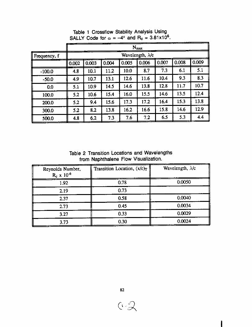
Table 1 Crossflow Stability Analysis UsingSALLY Code for c_ = -40 and Rc = 3.81x10 s.
Nmax
Frequency, f Wavelength, A/c
0.002 0.003 0.004 0.005 0.006 0.007 0.008 0.009
-100.0 4.8 10.1 11.2 10.0 8.7 7.3 6.1 5.1
-50.0 4.9 10.7 13.1 12.6 11.6 10.4 9.3 8.3
0.0 5.1 10.9 14.5 14.6 13.8 12.8 11.7 10.7
1(30.0 5.2 10.6 15.4 16.0 15.5 14.6 13.5 12.4
200.0 5.2 9.4 15.6 17.3 17.2 16.4 15.3 13.8
300.0 5.2 8.2 13.8 16.2 16.6 15.8 14.6 12.9
500.0 4.8 6.2 7.3 7.6 7.2 6.5 5.3 4.4
Table 2 Transition Locations and Wavelengthsfrom Naphthalene Flow Visualization.
Reynolds Number, Transition Location, (x/c)T Wavelength, A/cR¢x 10 -6
0.00501.92
2.19
2.37
2.73
3.27
3.73
0.78
0.73
0.58
0.45
0.33
0.30
0.0040
0.0034
0.0029
0.0024
82

Table 3 N-factors at Transition Computed Using the SALLYCode for a = -4 ° and Rc = 2.37x10⁶, (x/C)T = 0.58.
NT
Frequency, f Wavelength, A/c
0.004 0.005 0.0055 0.006 0.007 0.008 0.009
6.2 6.8 5.60.0
50.0
100.0
150.0
200.0
300.0
6.8
8.2
8.3
7.2
5.3
2.8
6.7
8.5
6.2
8.2
4.5
6.6
7.4
7.1
5.5
1.1
Table 4 N-factors at Transition Computed Using the SALLYCode for a = -40 and Re = 2.73x10 s, (X/C)T = 0.45.
NT
Frequency, f Wavelength, Mc
0.003 0.004 0.005 0.0055 0.006 0.007 0.008
0.0 4.7 6.5 6.2 5.0
50.0 7.3 7.6 7.4 6.6
100.0 7.6 8.3 8.2 8.1 7.6
150.0 7.3 8.5 8.5 7.9
6.4200.0
8.5
8.0
5.2
3.0
8.1
5.3
2.9
300.0
400.0
8.2
5.5
2.5
4.7
3.3
7.7
5.3
2.2
4.3
83
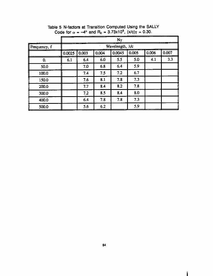
Table 5 N-factors at Transition Computed Using the SALLYCode for a = -4 ° and Rc = 3.73x10 s, (x/C)T = 0.30.
Frequency, f
0,
50.0
100.0
150.0
200.0
300.0
400.0
500.0
Nv
Wavelength, Mc
0.003 0.004 0.0045 0.005 0.006 0.007
4.1 3.3
0.0025
6.1 6.4
7.0
7.4
7.6
7.7
7.2
6.4
5.6
6.0
6.8
7.5
8,1
8.4
8.5
7.8
6.2
5.5
6.4
7.2
7.8
8.2
8.4
7.8
5.0
5.9
6.7
7.3
7.8
8.0
7.3
5.9
84
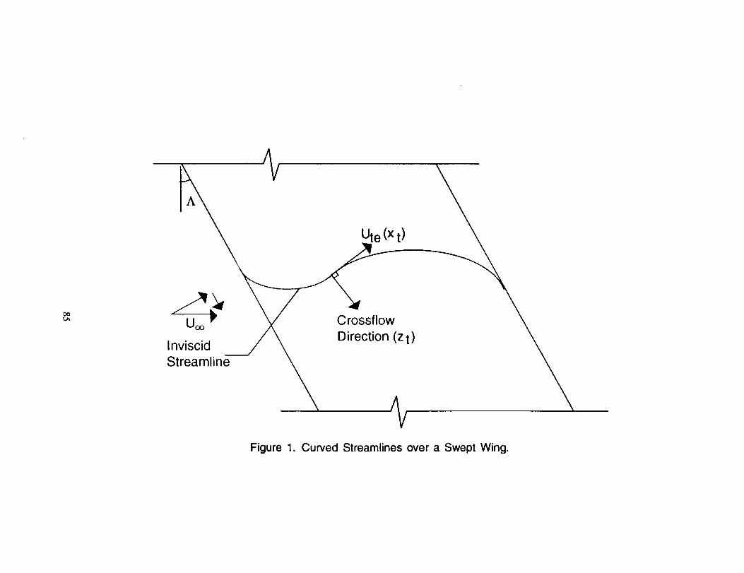
¢,.°_or)I=nO(1.)
0Ia..
85

86
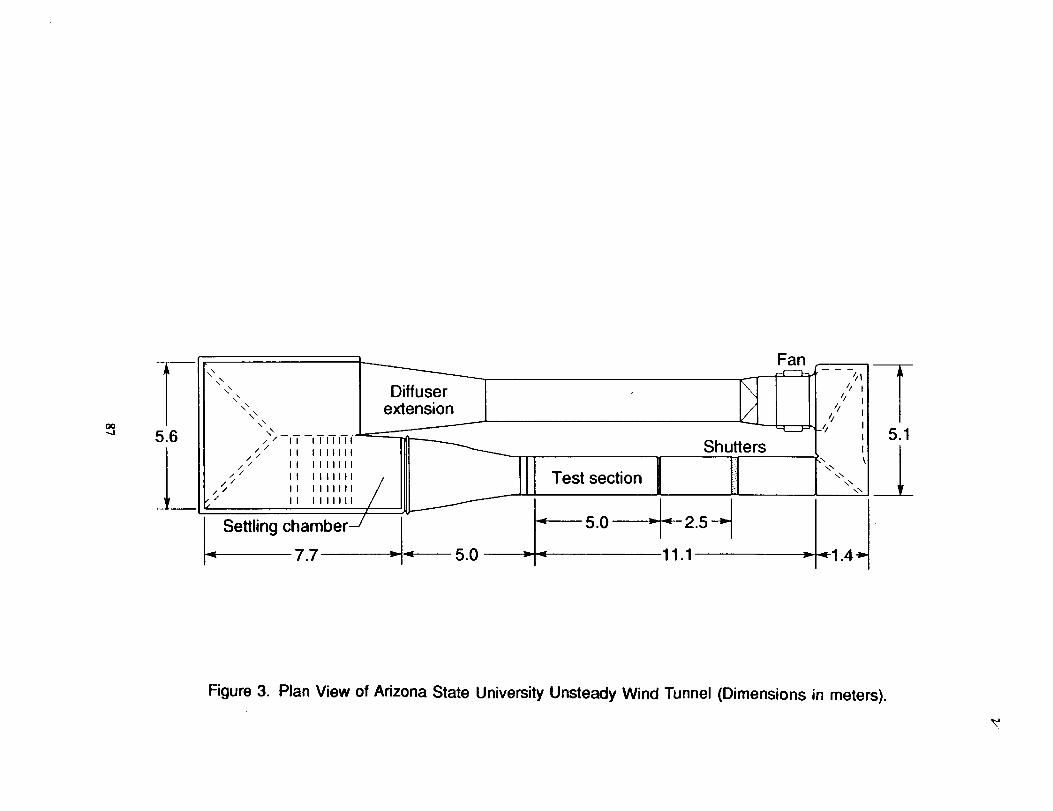
./-
I_Lr)
r
rmot-OoCc_
c_c_o_L
L
87

._o
2c0(.)
"0(.-
L_
c°_.-J
c0°_
z0e-e_0e-
0.U.
B$
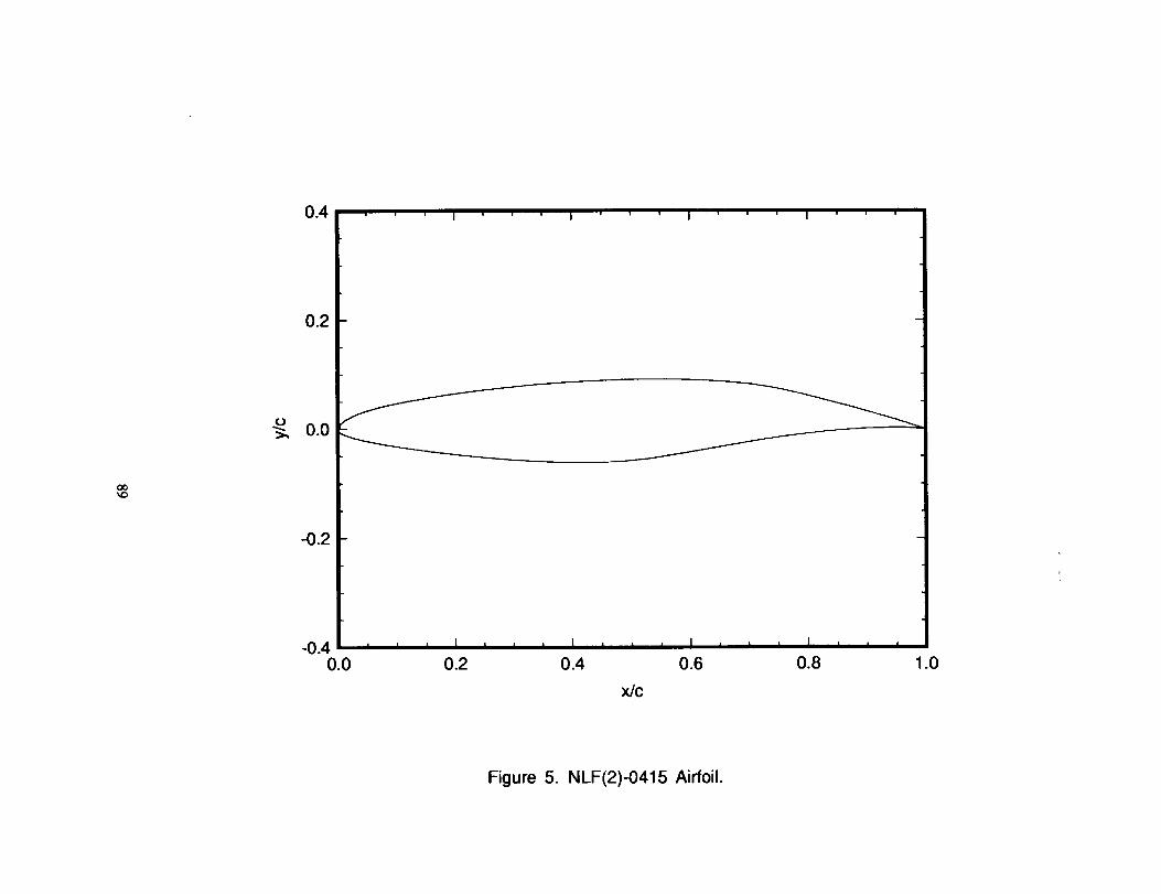
0
ii
ii
00
100000@
d0
,,
,I
i'
'0
o9
9
01,(
o_0°_90,,IvIi._Izii
89
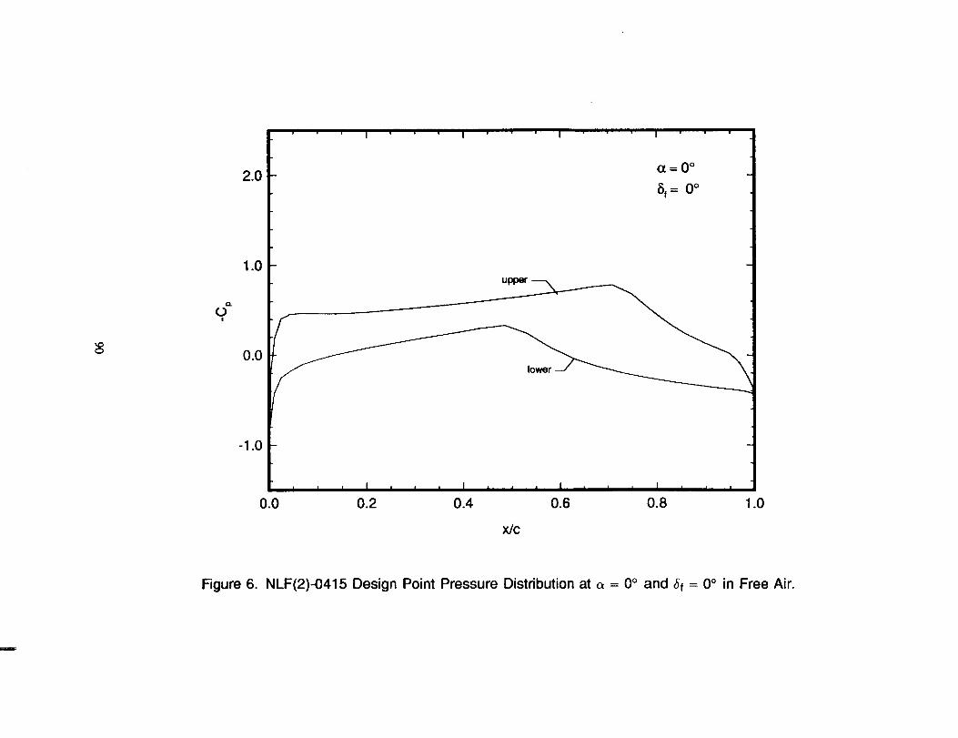
00
00II
II
0q
d0-
o
000
0cO000000
0u1.1.co0II
"000II0om.Q.l.-¢j')
o_au)(.-o_0o_u)
aLt_
9I.J...-IZI.I..
90

0_,°
IIII
_0-
!
0o00(,C)
O0
oDI.L.
°_0
IIw,.-
u_0
II
0WbD
t'-0.m.Q.mC3(D
0.b_T.m
ovLL
,.-I:7c_L
L
91

00
L_JO
!IIII
I'
'
llllllliil_ll__li
oq
oo
dO-
0cO0(4300C
_JQ0O
5.=
I1c0(3II
C0
II
0e-0.m.Q°Br_5_
a.L_,g...
oAL'MIt/ZU
.
92
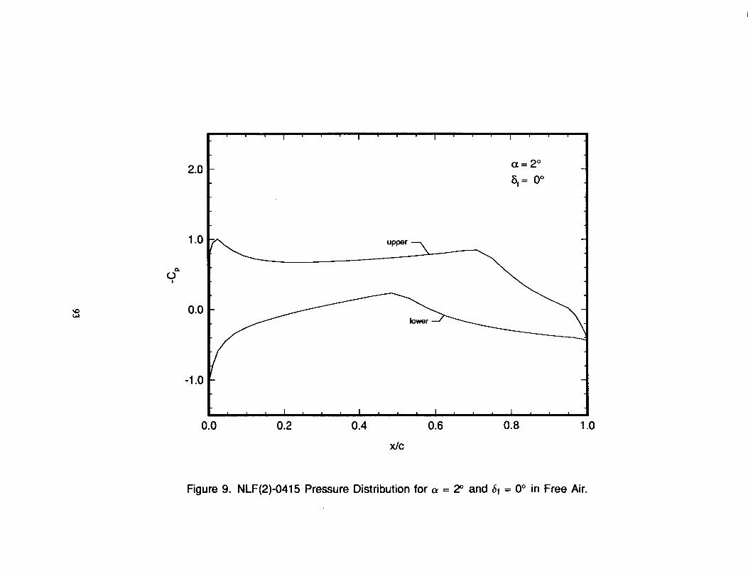
00
do.
00
0
OcO
0_0
O000
L_
,m
LL
._o0
II
"I0
f-
&II
0t-
O.0
r_
O.
uO
oCy
LL
..J
Z.__U
-
93

0o
0
IIII
o
!q
dO
00
!
0
0cO0_D00000
om<U..
°_00II
00II
00.Q-c-
r_noLL--JZd°_U-
94
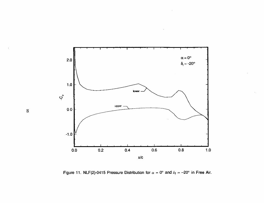
o.OJ
|o
o.
dO.
00o._rm!
0aO000O,I
000
lIE°_eLLC=
°_0C)II
"(3ci
00
II00°_.r-
aenoLLI
ZTm--L
°_LL
9S
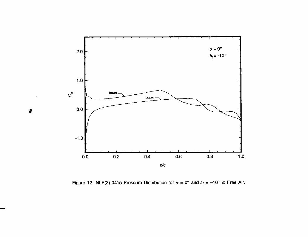
''
I
0O0
'T-
O,
IIII
0O4
Tm
IIo
C_
C_
I'
'
C_
T7
',r--
GO
C_
C_
C_
OOC_
im,mLI..
°_00
III
"IDt.-
0C_II
in0i.-0-r-
rmnoAvU-
--IZT
mC_
°_Ii
96

0(%1
dO.
q0q
0aO0(000000
,<(Dq)IJ_
°_00II
"0c--
0(:3II00°_"Ca0..IZ)
9v14...JZ(3)°_LI.
9"7

0
o0
UU
cJ0.
!0q'T
0cO0¢000000
,D,,<LI.t--"°_00II
"10c00II3c-o0_.a.r-aI1.
14")
9vLI..-.IZ4°_I.I.
98
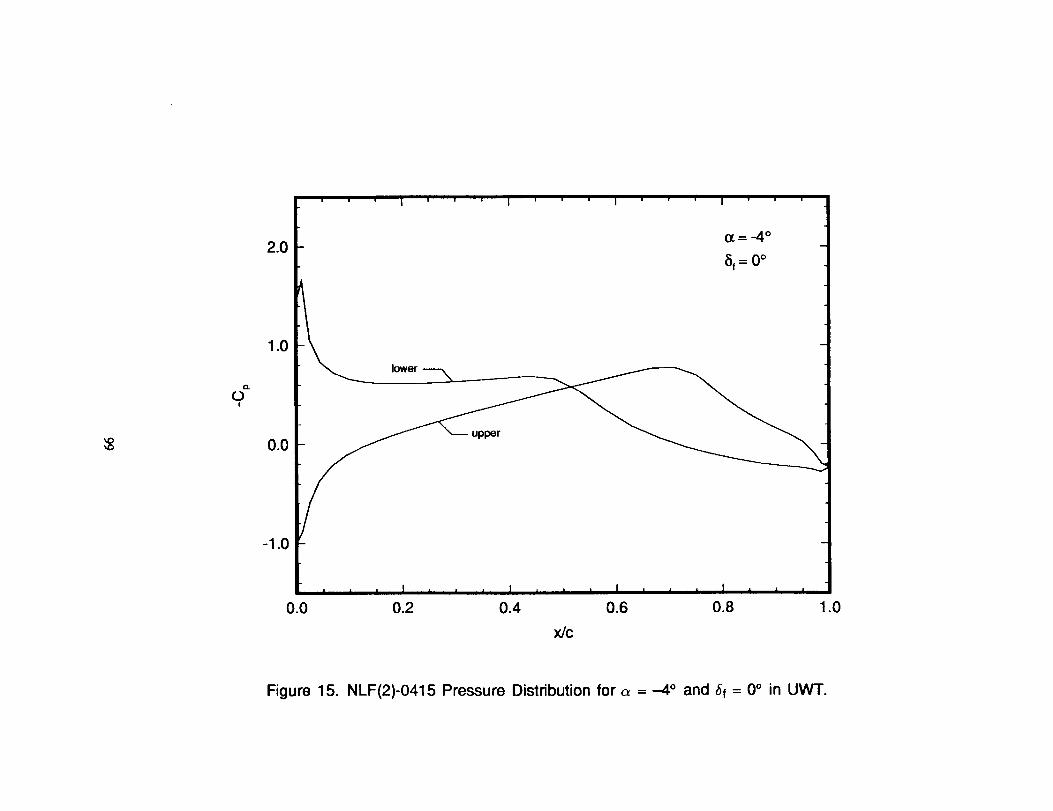
0IIII
0o.*itm
00
O
OT=
I
cOOO0C,I
0O0
t-o_0OII
c=
0
II
0t-OoD.Q"cz
C_
0.o,
vLL
.-JZL_
Tim
c_o_U
-
99
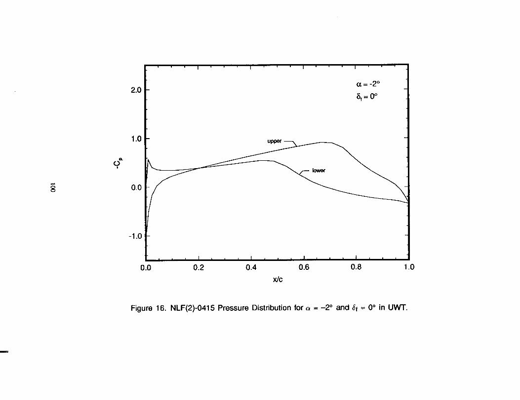
0IIII
q
!
0
I,
i
0
dO.
0000000
o_00II
"I0t.-
0IIL_00.0,r-ac_
Q.
0!
AvI.L..JZ.__It.
100

0Cxl
0
d9.
o.Oq"7
0cO0(D0O¢Xl
Q00
°_0OII
¢-t_
0I1
0¢-0.I"t'-
tOo¢xlvLt.
Z0_
101
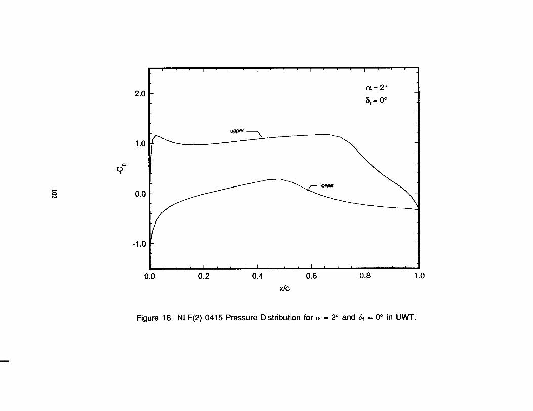
00
C_
0II
II
q0
_0-
o.00-r
00cD00000
e-II
"0e-0CMII0.oJ_
-r-
a"-1
p9Cxi
U.
.-.1z.__U-
102

00
IIII
|
dO.
0000
t-0_00II
0IIt,-0t,i.-{-0.IC_
O.
IZ)
0'..L.¢qI1iJZ°iU
.
103
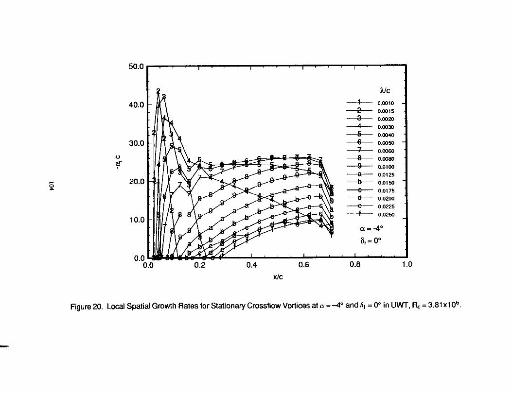
II
II
_.8.8.8..
.o.o.o.o.o.o.o.
OO
OO
O0
00
Q0
00
0
0
II
II
000
0_0-
co0xcOII
c00II
t-o"TII0,9.oC
)0o_0rrp(1)
..IdI.I-
104

o
II
I
888888888qqqqq_
00
00
O0
00
00
00
00
0
00
0o
0o
dd
dd
0_0-
IIII
0000_D00000
od
_D0xcOIIc:00
II
c:II1
U-E0o0c:00co
rr"o0._Q.
cO0._1
O4e_IJ.
105
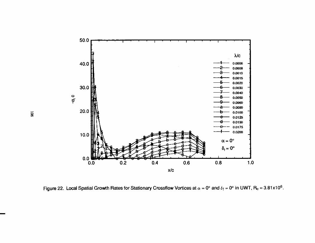
iI
ii
888.8_.8_o
......_.qqq
..
00
00
00
00
00
00
00
O0
0
00
IIil
000
0xcoH00II
e-
00U
?,0e-oo_L_
0ffl
n-ai
106

II
II
00
00
00
00
00
00
00
0C
_l0
IIIJ
0cO0000
_D0xcOoiI1
°_0C_II
00,,I00ot-oO0o0_e'--
oCO0,_J
o6_3
LI.
107
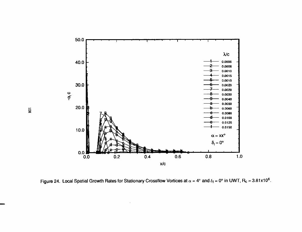
II
iI
_._8._._.8.8._..8.
.....o
00
00
00
00
0O
00
0O
0X
o..x
0cO0
J(D0
JJJ
(D0x"t'-"00II
°_00IIr--
oII(_0or-o°_t.w0w)..,-
(n2Q.
..J
108

''
I....
I
_$_8_°_°_°_
00
00
00
00
00
00
00
00
IIU
cO-
(OlX)N
qCO
0
0xCO
c')II
rrt-
oo
II
-OoII
.o
ot-O°_00_6
°_
I09

o
•'
II
0......
00
00
00
00
00
00
00
00
(o/X)N
_bIIIII
(3CO
0
QxcOII
o0II
"0t-III90.90Z0_U
.
110
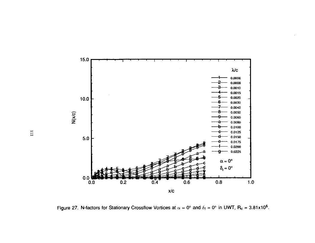
00
00
00
00
00
0q
oooo
ooo
oooo
o0
oO
0
(o/X)N
111

q
II
SSS
S.
._.0
00
00
00
00
0,0
00
oq
(0/X)N
00
liII
0X
0C
OII
O0
_-0
o0II
"0t-¢1
(.IOo<1)0
0
0
0c0O90
,0
0
dZ._mU
.
112
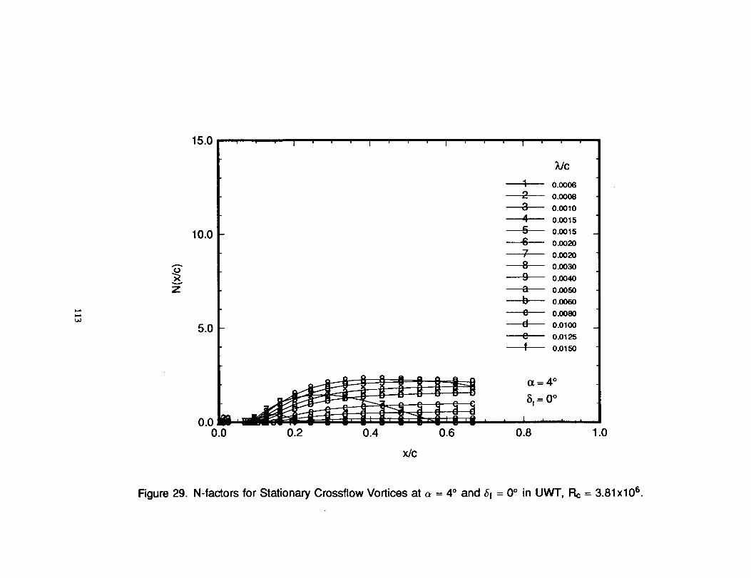
x
QII
(O_)N
113

0_.°0
IIII
00
0d
_'_N
0d
0xII
¢.-,_00
II
dc_
oli0
0d00
O0d
Do0t_
c0000zEE°_
c5
cOLL
114

0u./
,i
vI
•
0_°Q
UII
i10d
'I
'
II
O
II
I
Qd0Od0d00O
0d
Qxa_II
c°_0QIIII(#)
00mpOZEEx=!0_I.l.
115
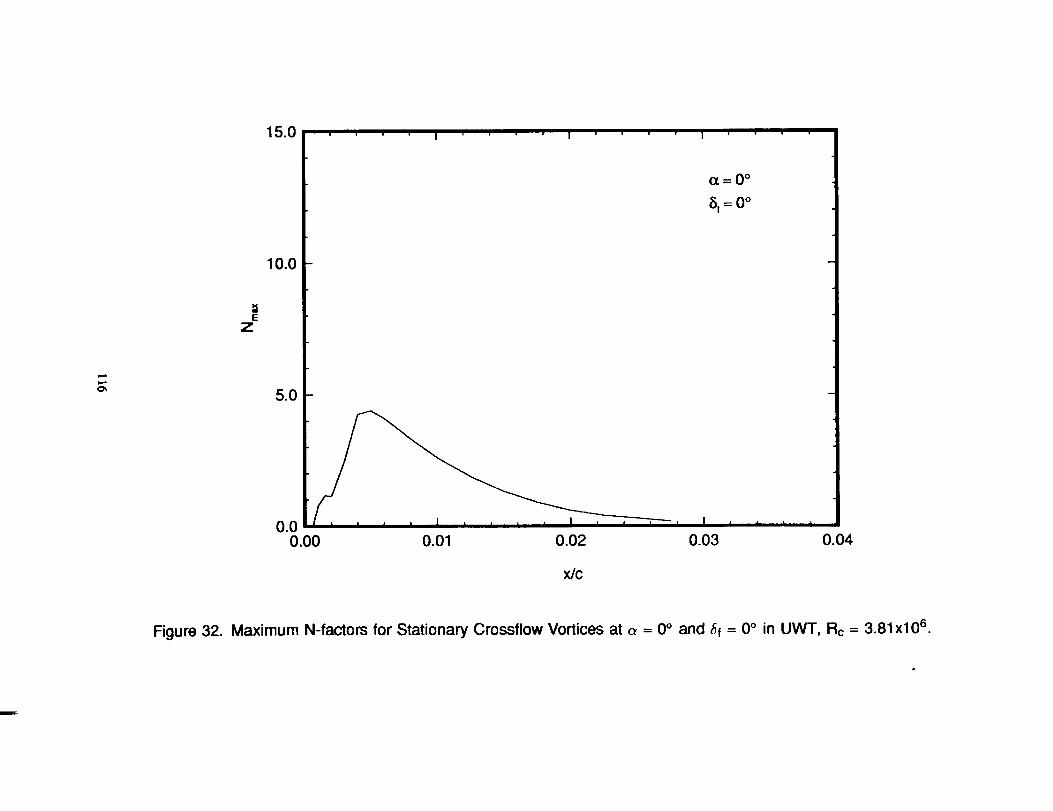
00
00
IIII
0
_00xaO
,_.II
d
116

0
0O
IIII
II
II
lI
0c_
_"'N
ai
0u_
(&)0xcOc_
_I"
II
dn-t-
o0
II
o.
_0
0c-
o
II
Q)
d
_o
0._o
d
O_00
o0oo
Ed
E°_xc_
cO.m
U.
I17
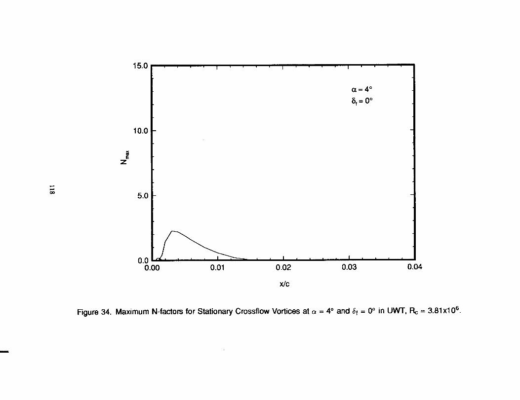
0
@0
UIt
II
Ii
I,
00
_,wN
I0LL')
II
II
118
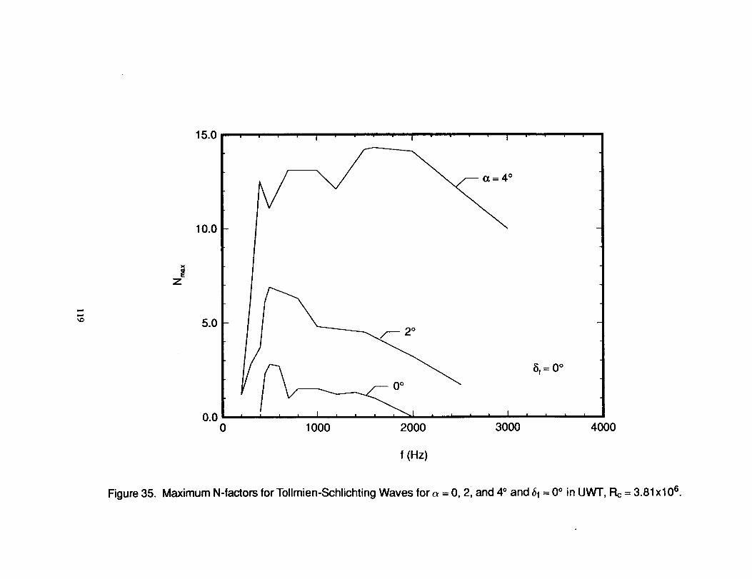
L6
T"-
0
II
I,
Idqr-,"
I19
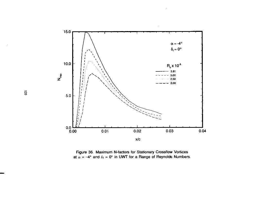
0IIII
0CI_
IIII
/
/
_wN
dcO00
(I)
OJQ
_E
e.-
on"
.0_..rr
_-
0
cO
U.
120
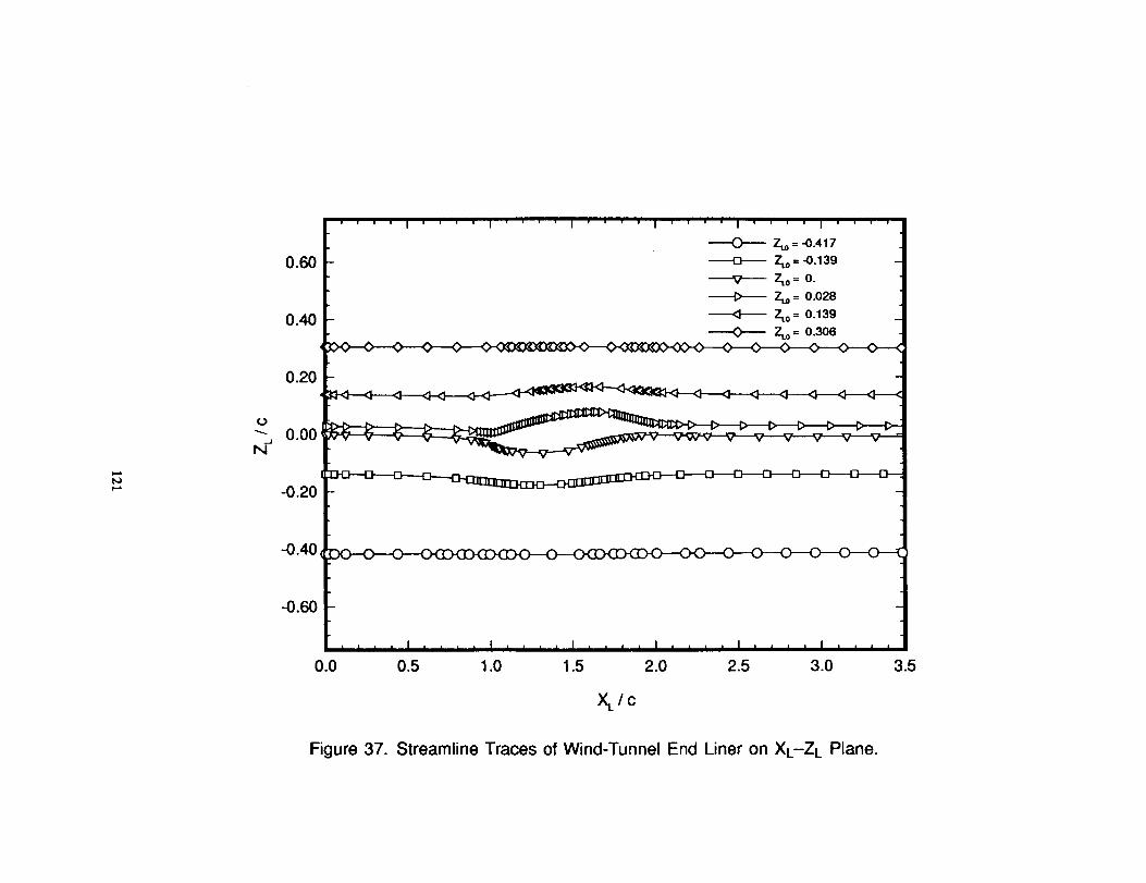
0
09
0o,
8o
CO
003004
0000
0x_
¢-
13.
.--I
N,_J
x4--
0_=
°_.=I
"0
LLI
t--I
I--6t-
Ol-
iE09CO
LI=
121
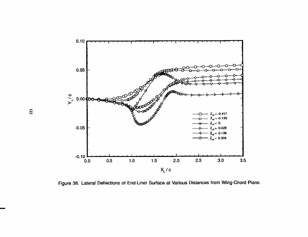
0
x_
e-0e-9e-°_Effl
e-
aP,"e-e-°__.16¢-0e-0o_a_.1
122
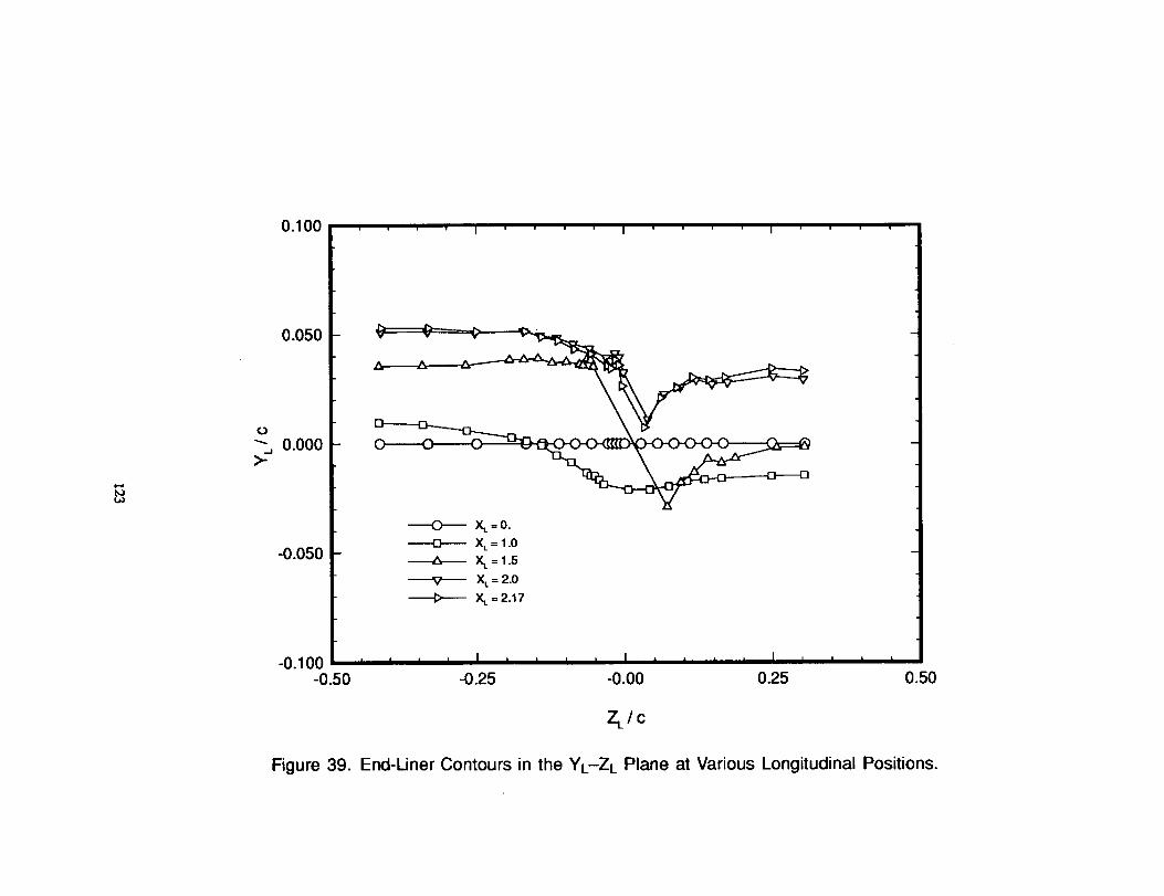
000
....
I....
I'
'J
',
,,
/I))
I
)
r_o
_o
IIU
IIII
II
ttt,t
00u_00¢.)
09_
90
00
00¢_,
oo
o,-
oo
99"
0/1A
00ne-°_"0t-O/U
)
gQ)
cn..J.d
>-Q)r-t-Ot-O0Q)
r-r-uJo_C
O-iO_
o_I.I.
123
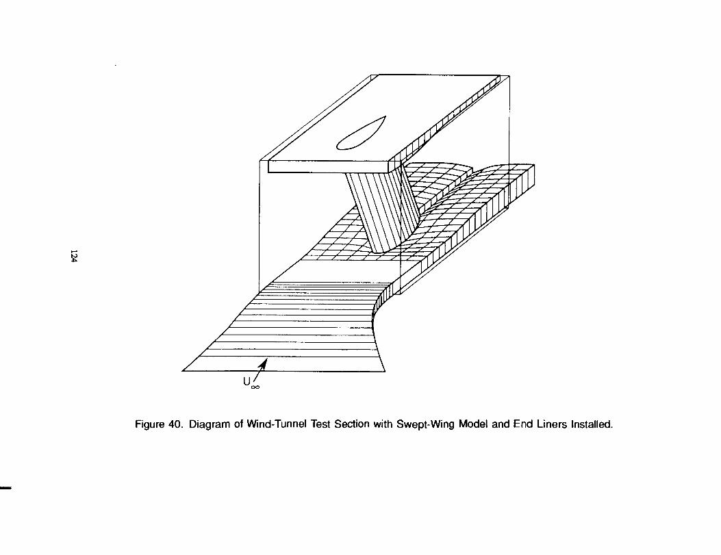
\
iiJc_EC_
c_
t_c_c_o_L
L
124
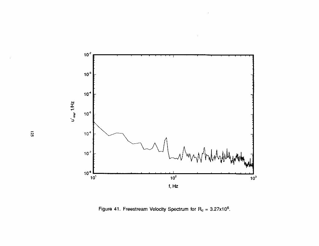
toOX03H
rroE0EO3
0U-
,_U-
ZHI
I."'_,n
125

0Q
0o
0o.9cdO.
O9
LUn
O9"
Q000Or,O0
0
O0O080
0
"100II
"0,-."
G)
(D•,.-"
"0.0
0
.o_0
0_)t..-
t--.,-,
0.,-,
.:.-E.__
0o
aio
,,_-0Q.
126
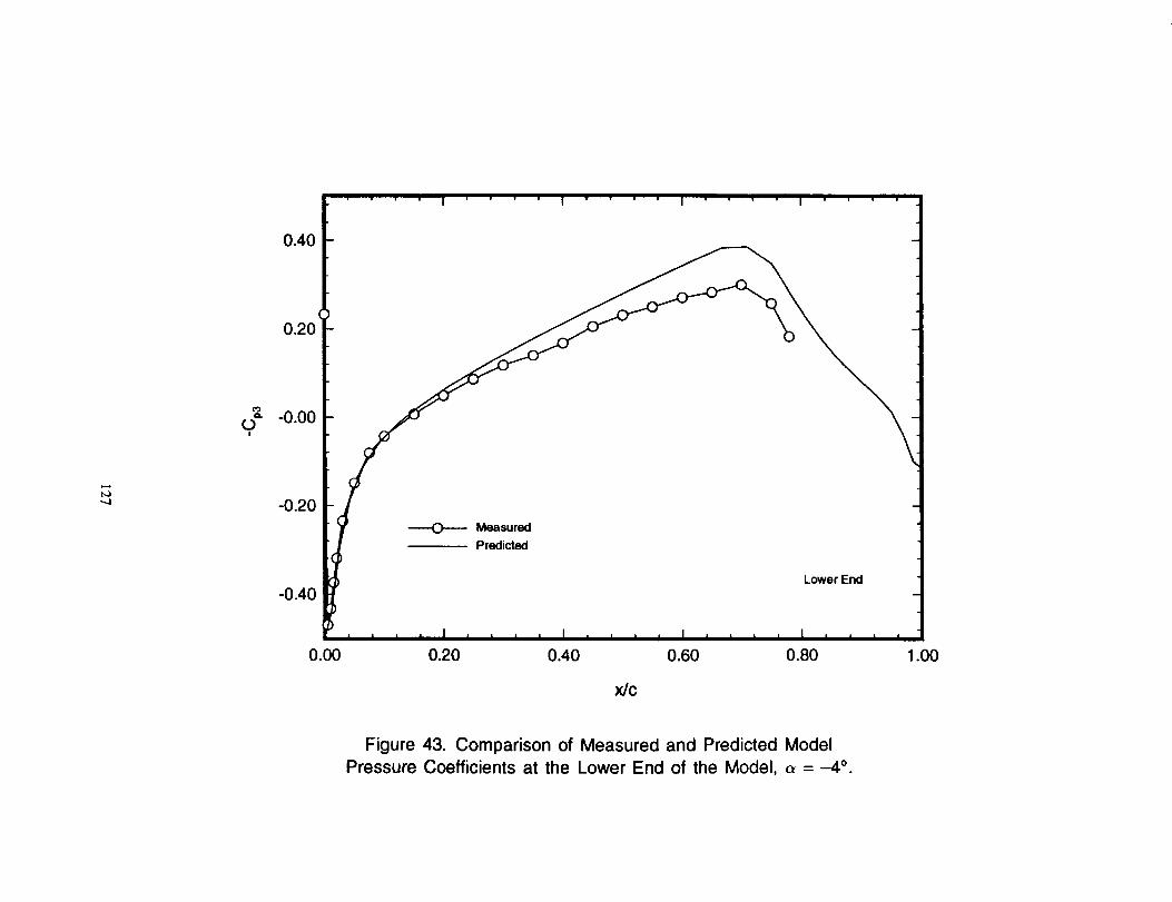
00
00
0o.of:d_).
09
o9
000co00_D0000080
o
"00II
"0---"
_-""0
•_-0
nca0
ca
_o._Jt-
(-4._
0_--
.__ca
ca_0
O.
_-E
.-0
oa__o•-_
_n
127

61/16/89 RUN6 R = 1.93 X 10-
c
Figure 44. Naphthalene Flow Visualization, <_= -4 °, Rc = 1.93x10⁶.
128

61/16/89 RUN9 R =2.19 X 10-
c
Figure 45. Naphthalene Flow Visualization, a =--4 °, Rc = 2.19x10⁶.
129
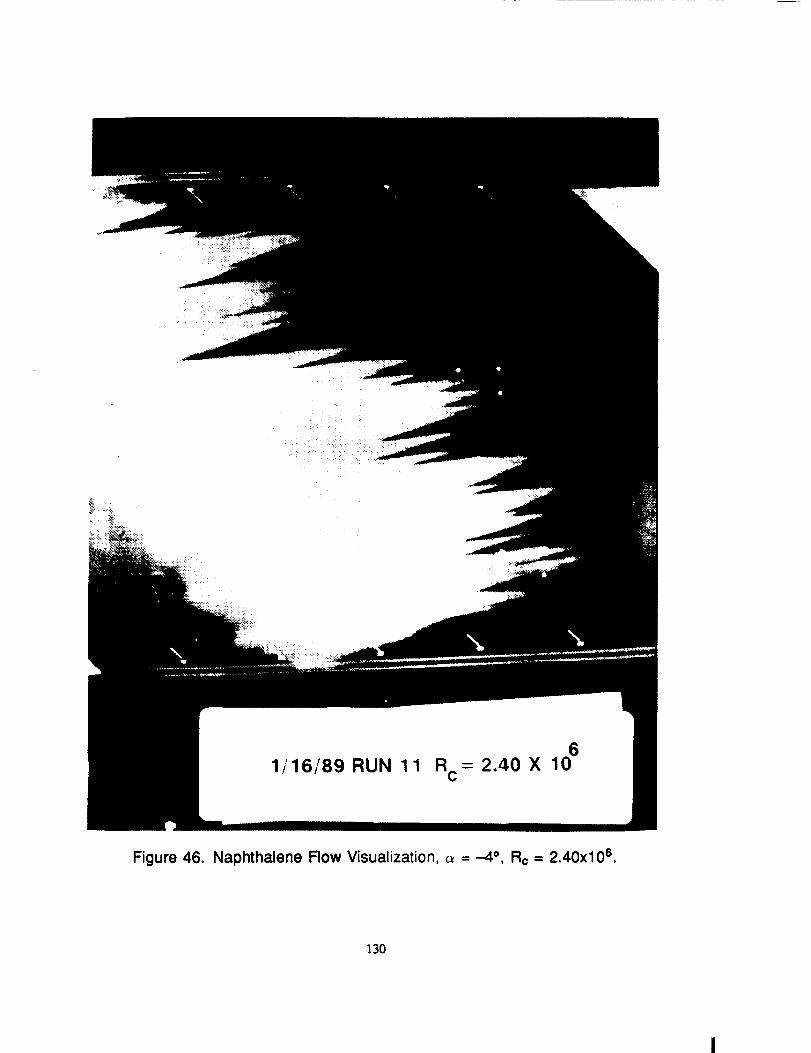
61/16/89RUN 11 Rc=2.40 X 10
Figure 46. Naphthalene Flow Visualization, c_ = -4 °, Rc = 2.40x10 s.
130

1/16/89 RUN8 RC=2.73 X 10⁶
Figure 47. Naphthalene Flow Visualization, c_ -- -4 °, Rc = 2.73x10⁶.
131
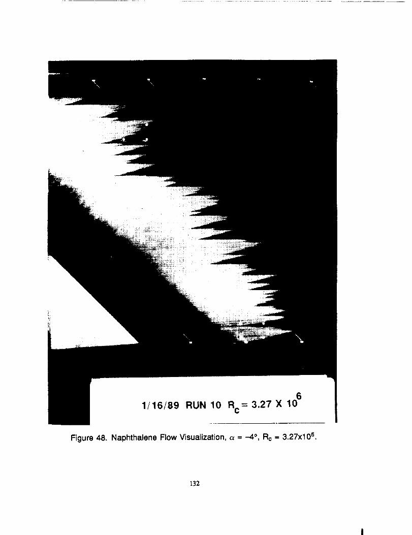
1/16/89 RUN 10 Rc=3.27X 10⁶
Figure 48. Naphthalene Flow Visualization, _ = -4 °, Rc = 3.27x10 s.
132
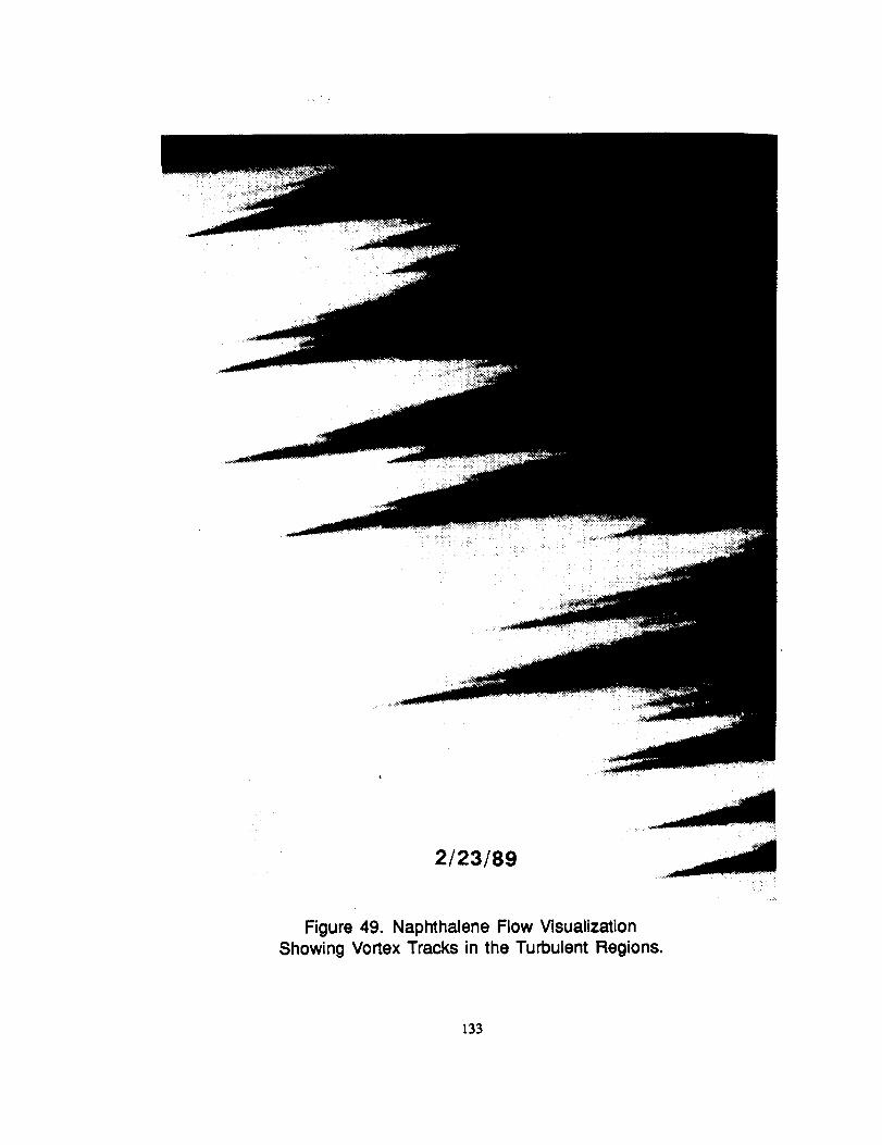
2/23/89
Figure 49. Naphthalene Flow VisualizationShowing Vortex Tracks in the Turbulent Regions.
133

ENOI!?:3._"
.Jdu')
O)
ii°_
134

I'
''
II
I
Z.1..
z
<_c
p-
<1
<1
I-q
00
0Xu
n-
0
EZ0rr(/)c-O00.-It-Or-
IZ)-1U.
135
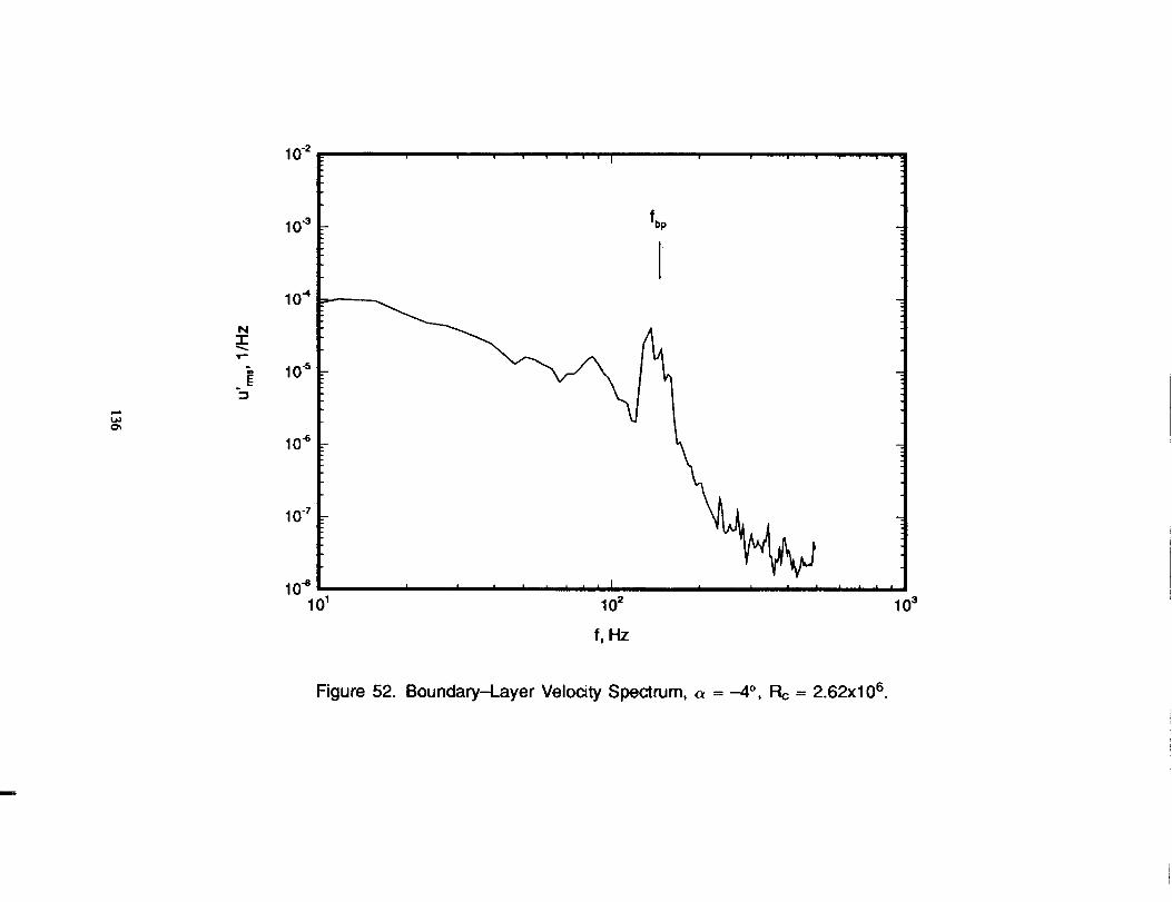
.......!........
I........I........
I........I........
.0
0
01"'*
X¢Dc_II
0IIE"
2o"oc-Oenc_3°_U_
ZH/I.
'*"",n
136
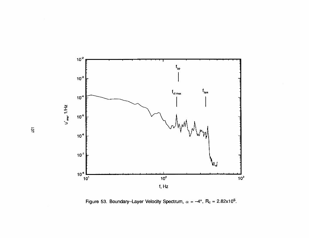
lillI
II
Q
I........I........
I........I........
I........
illlll!'
'_1
........I.......
,I........
I........
00
00
0
0
_00xO_
cO
o4II
07II
0"0¢::::30rno_t,O
o
ZH/I.
'_,n
137
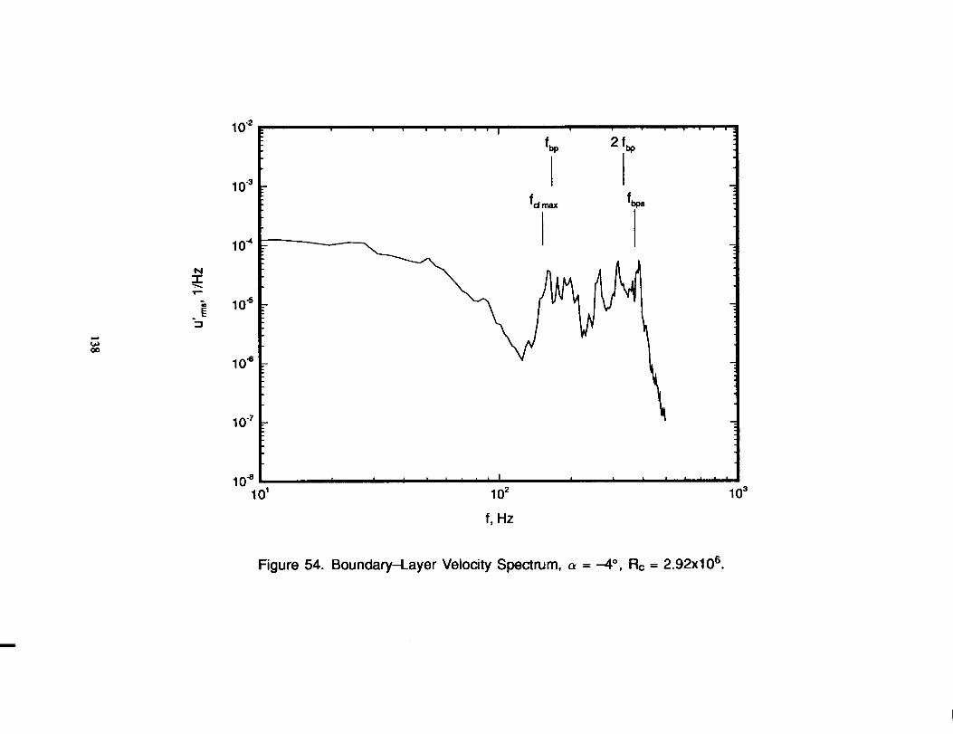
........I........
I........I........
t........I........
3Q.
f
J
|Jilli
•|l||tll
ii
OO
Q
QO
OO
O
T"
oT"Xe_J
e,iII
@?ili2Or}
OC-'1OI:I:)
--1
o_L,I.
ZHII.'"'",
n
138
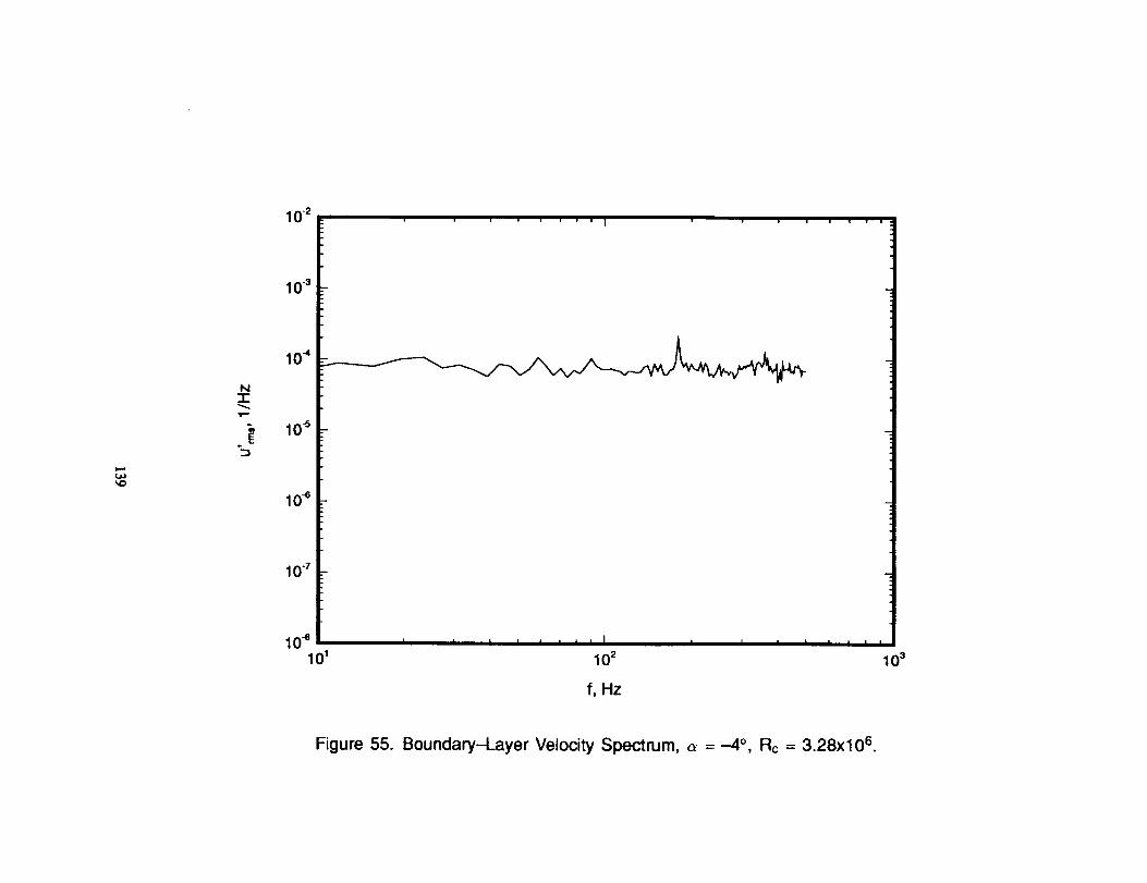
........I........
I........I........
I........I........
I|lllJ
ii
|llJJ,J
,I
,"?Q
0
0
0Q
O0
Q_
__
.s.=-
N
o'S""
XH0liE{/)o"o"s0"-s
I.I.
ZH/I."_,n
139

ii;UJJ
_
ZH/l
,n
0
_i_°
Q'i,,,-II
_ZO"
TII
"40
1:1.
00.r-.
E0
bT.
140

0
0CY
Oxf4_IIU
rr0"TII
o"QII
uomonuoORELr)
3I.L
141
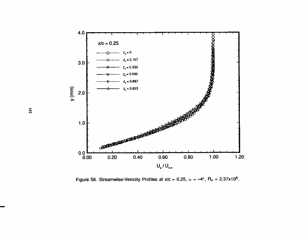
I....
I....
I
•0
0d
do
od
oII
IIII
II|
U
0000cO000000....
I....
I,
,;
;I
;,
,,
0
o.o.
o.o.
oo_1"
_O
J_'-
0
CO0xp,.II(3n"II
o4o
Uu)_oo__oO
.
.#=d
8E41==wU
3
IJ_
142
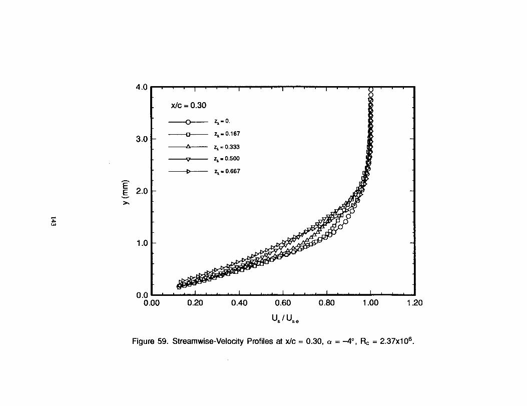
0
O00
(.D0xII
oTII
c_0II02nr..)oE(Dc__m
IJ.
143
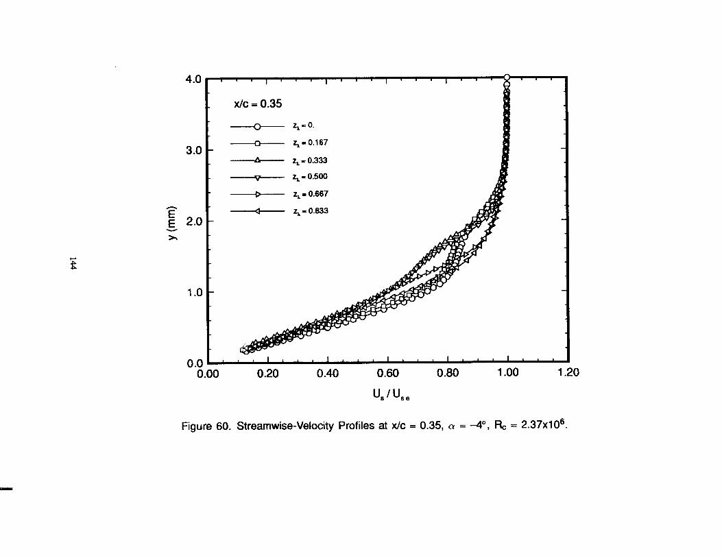
0
°°
•d
do
od
oII
IIII
IIn
II
(ww
)
C,OOxil
7_II
c_OII
83Ec_C_
o--

o
I'
•'
'J
o
I"0
to0xr,,,
coIIo
rr
0
U
c_
_rc5II
.o
Q.ooEGOco
.IU.
145
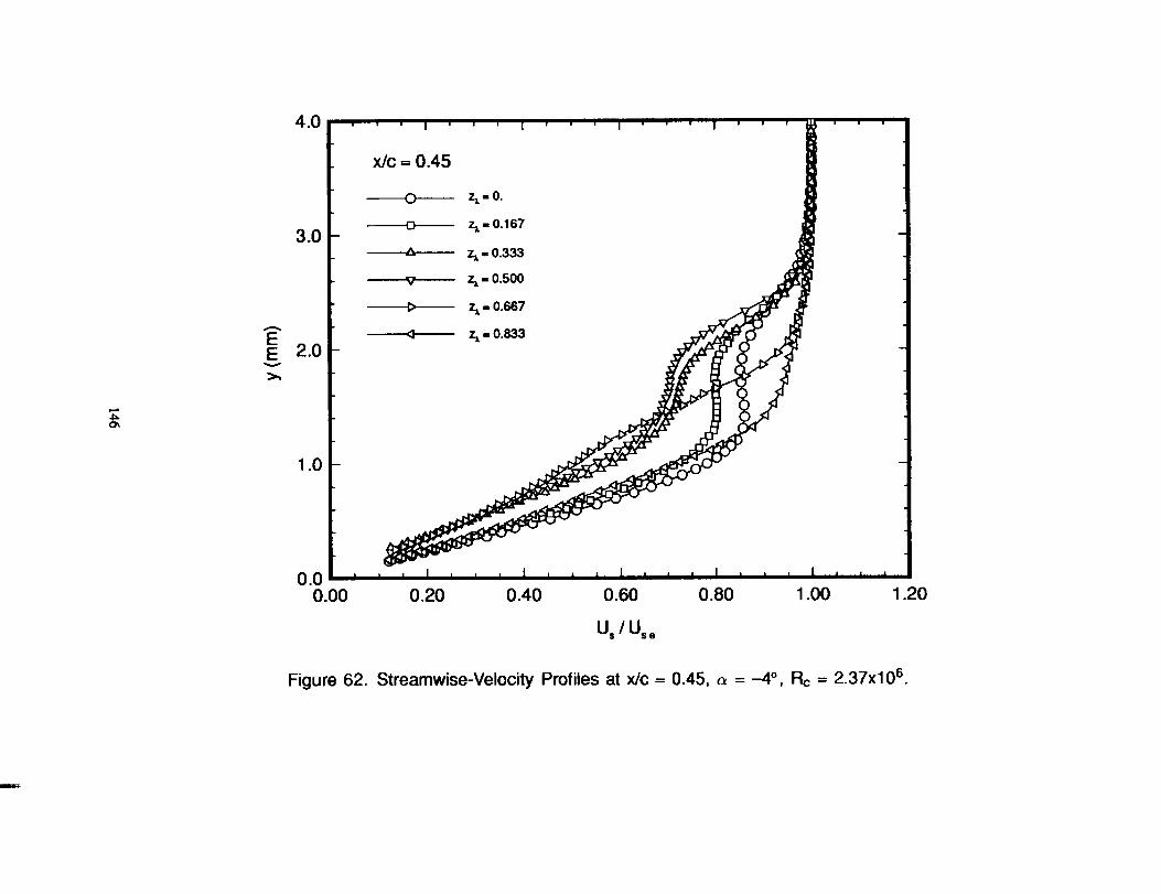
oQ
.q
o
8ocOo
m
oo0oc_oooo.o0
_o0XCO
oJII
0II
¢3IIin•o__0°_EoJ_0°_LL
146
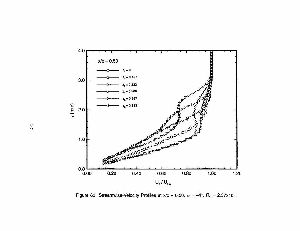
o
II
1
0
oo0cO
00000
0xh_¢0H
0
II
c_
0
Hq)
o•o00
._EcO
O0q_
LL
147
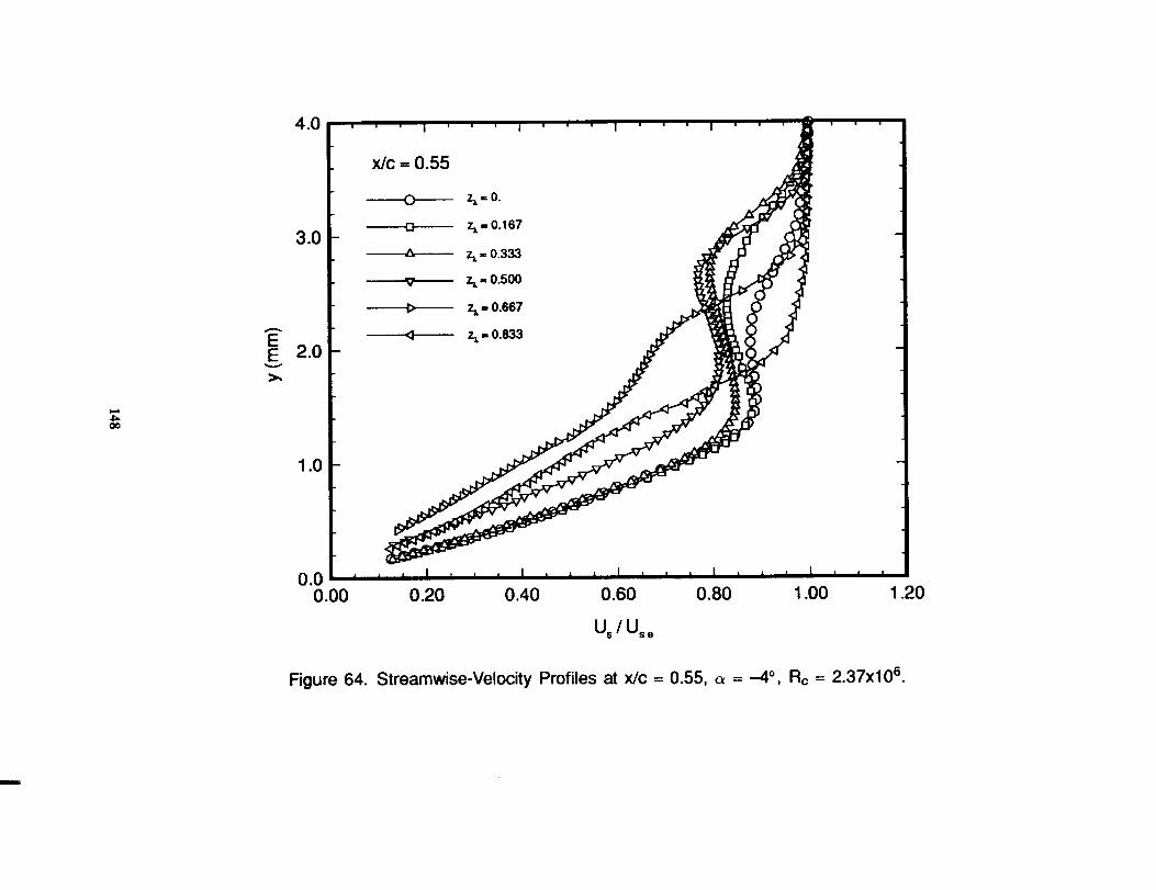
0qC
Oq
(ww
)
o.
0000000
CO0xD
-.cOII
n-o"IIII_o
noo_EO3c.0
LL.
148
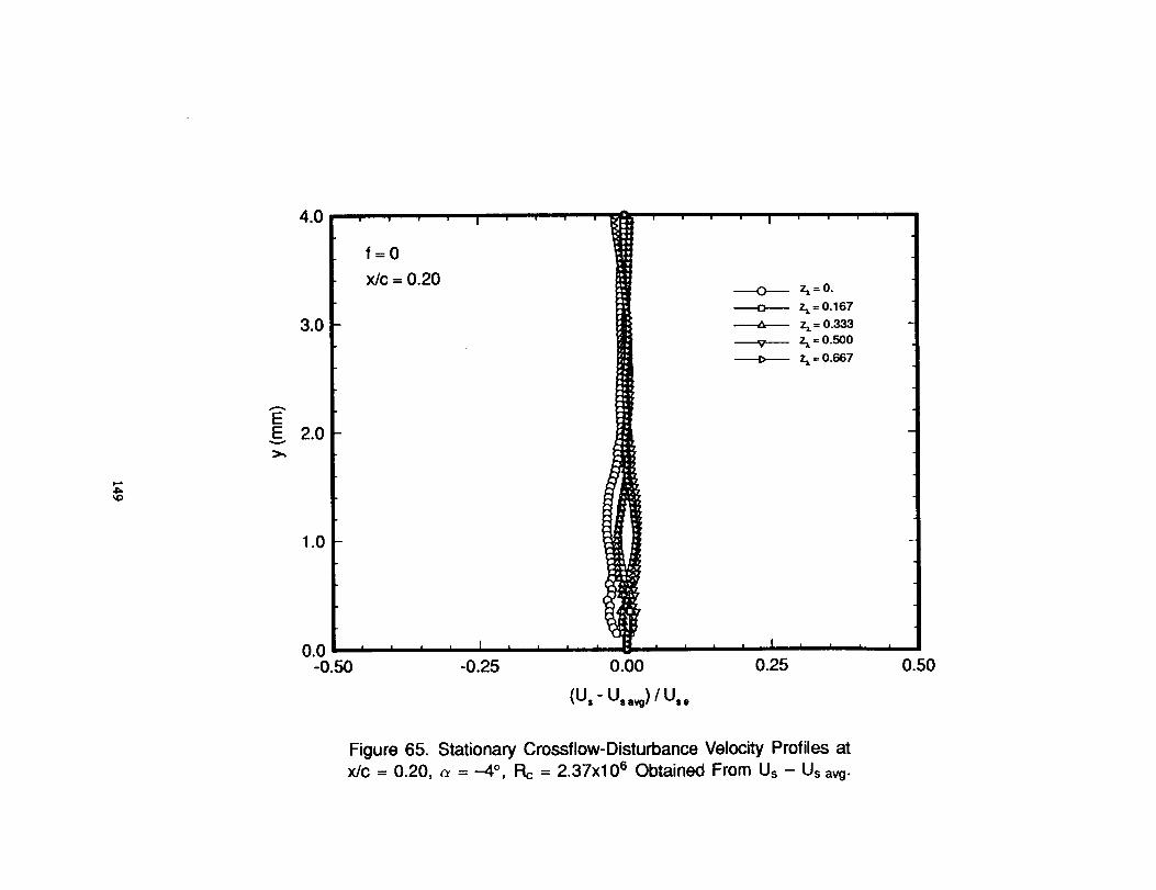
I....
I....
1
dodddII
IIII
UU
tttf
0I,l')0<,>
E"_8.o_,,
0,
,,
,I
i,
ii
Ii
ii
iI
i,
,,
oo
oo
o9i
(ww
),4
149
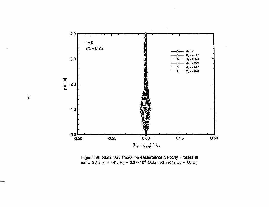
I"
dd_od_I|
UII
n#
H
00Lt_
00i
d0
II
,,
__
Ii
ii
ii
ii
i'
i....
oo
oo
o.9
C_o
II
_d
(ww
)
150
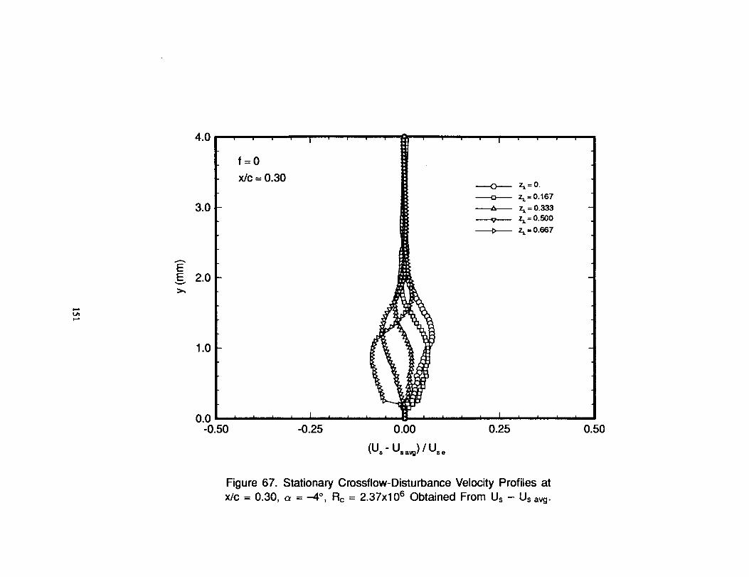
0d0
II
0
oo
oo
o.9
(.0d
(ww
)
151
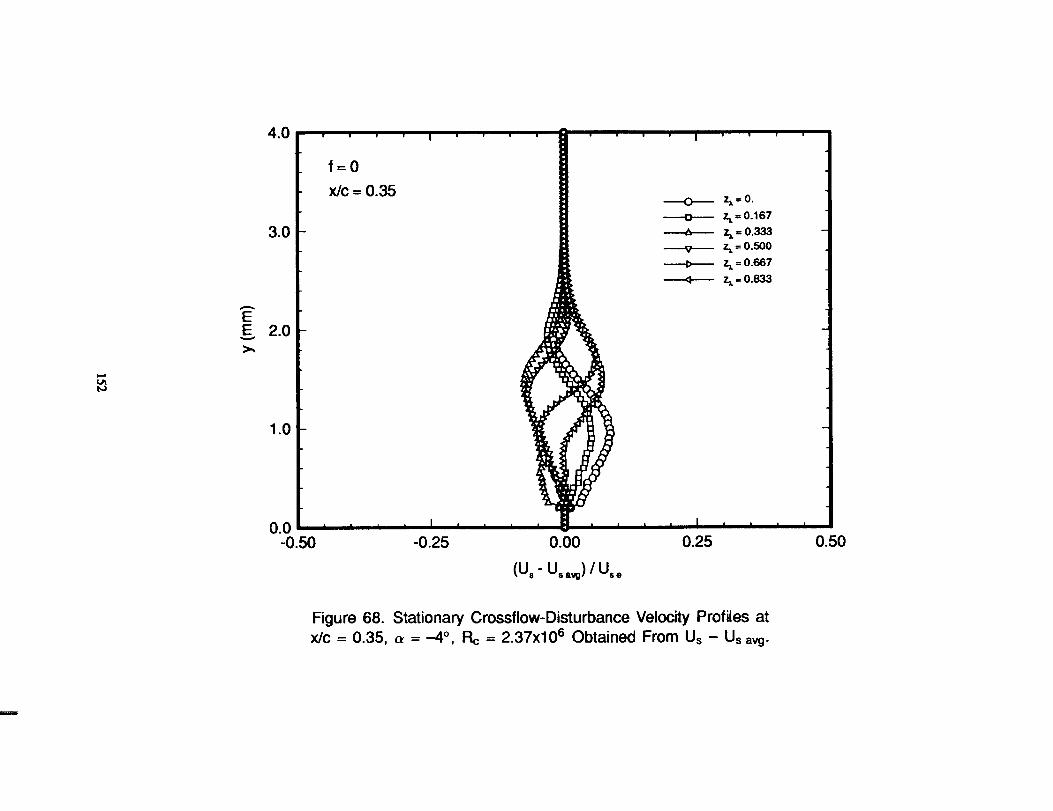
....I
....I
c_c_
c_c_d
dII
IIu
IIII
II
ot.oodo4
(ww
)X
n
70o
t-°_
=0
aoX
oP,_
_u
g't°_(D_d--1
U
152

'I
II
oc;dddd
II
II
UII
II
II
IIII
0I.¢)
d
_o
00
0II
I.O
90,
,,
,I
,,
,i
I,
,I
iI
I'
''
oo
oo
o9
"_oi2
ii
_io
II
_d
(ww
)
153

II
I'
I....
I....
I....
154

I....
I'
'I
i,.,.11"]#0
r,,.(_
"_-E
2"
0o
tOo"
o_
_
o0
II_
d,-
_&
"
,,
,,
I,
,i
iI
ii
ii
Ii
I'
'
oo
oo
q9
(ww
)
155
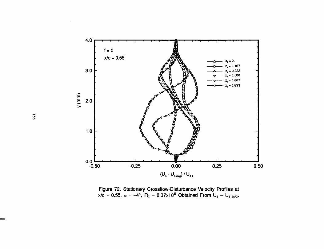
I'
'I
I4_
c_c_
c_oc_
c_rj)
mII
I|11
IIII
li(_
(.')
-®
-_
-e-_
da,_
Ng'r
u_b,.
o"
_md
_-:3
II,,_
_._0
ii
,i
I....
I....
J....
00
00
00
•I
_:
__i
,-
o
(ww
),_
156
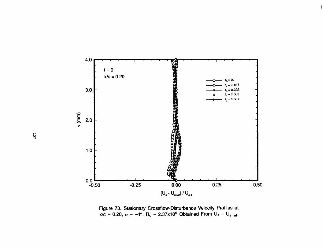
IIU
i!II
II
J'
._
,
0L_c_Lr_C
_J0c_
I
J
Lt_O
4
o,0
0C_J
d0
II
,,
,i
I,
,i
iI
lI
''
I....
oo
oo
qO
(ww
)X
_mD"10
c_.,-,
-e-a=0
b,,0
157

II
i
dd6c_dd)l
UU
14O
!il
tttt
0
J
0"---E
i.r)c%
1d
0II
0
o0....
I....
I,
,.
,t
o.
,,
00
00
OC
t,
(ww
),(
158
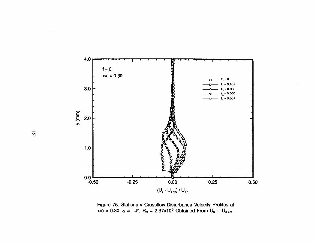
(ww
}
159
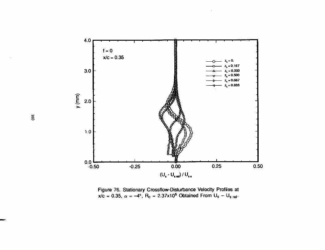
I..-0
°0
odooo
UU
IIX
IIX
t4t,t,t
|'
''
'I
''
''
ot_oo
0
eii
o
&
oo
II
o,
,,
,I
.,
,i
l,
¢L
iI
i¢
,i
oo
oo
co,
160

i....
II
i....
d
i|II
IIII
Un
n
d_.,:::)_Eo9-_LL>'0
®rJ
r-
-g8
d_9_"_ai
000
II
0I
''
'I
....I
....I
....I._
oo
oo
o9
(/)
r,.•
o
--so)o
LT__
(ww
)
161

II
It_
,,I",,,t',,_',,,F',,1",,,I"
_I
_U_
®¢_
e-
•_
_g't"--
II
oo
II
oi
i'
'I
....I
....I
....
oo
oo
o.o,_
_,--
o
o
162
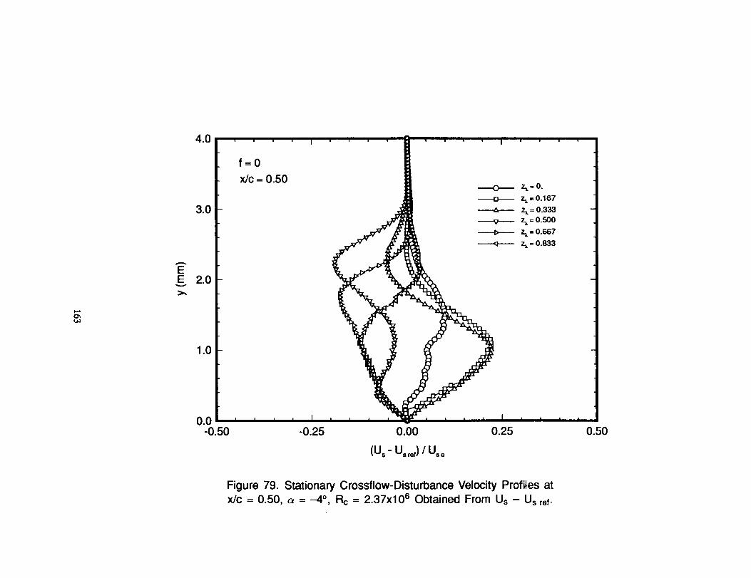
163

oI
II
II
....I
....I
....
oo
oo
o9
(ww
),_
164

o
i'
....'
'i_
I__
1I
nn
nu
nl
I-_./III
¢-4_
olillt
,,o•
_J
_
J__5
oo
oo
oc_
(ww
)x
cOI.I.
165
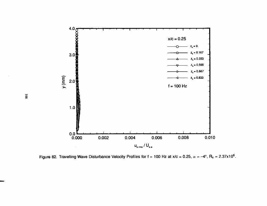
e4oOU-
166
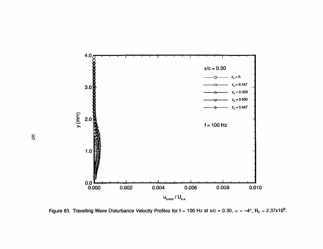
II
I
¢0
o¢D
Nu
Nu
U
oII
NI00II
000000cOooooc)o0dOOO
cn
oXcoo4II
OII
c_¢0oIIN7"OO,1"-IIb--oQ
)
n(Joocco
33l...
N°_
8oo
oo
o.
oo
•_"
CO
Od
T'-
0
(ww
)xl--co
167

oII
I'
''
I_-
IFc_
oo
oo
ot
J
_5
8o
oo
ood
c'_"
CO
(_1't-
0
(2O
168
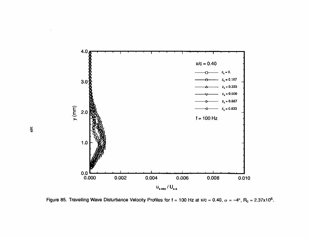
_DcO0")LI.
169

_D
I'
''
1o°i-
od
oo
od
4II
I.
,=
""
=I
mII
ft.
o8
oq
o.o.
Qo
I--ooLI.
170
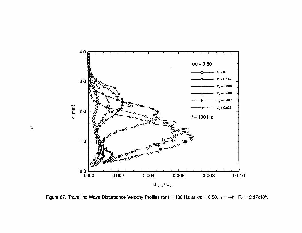
o
IIN
IIII
U#
(ww
)xl-co14.
171

qD
0
I''
''
!o_
Ji-i_.
too
r,..co
1_D
0tO
I"-_'
__
II-
do
oo
od
JIII
d8
d_,8
d®
"-
_2
d0..
N8t-
O
NN
8O
(ww
)X
00
cl--cO
172
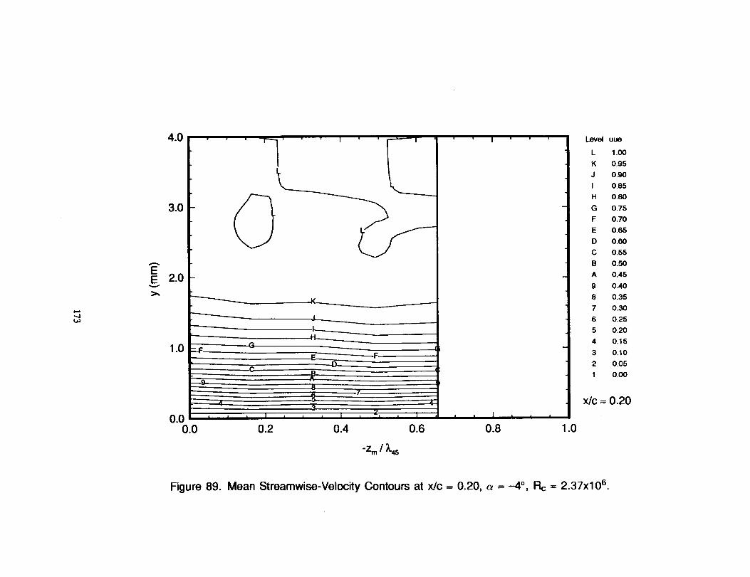
___00
_d
ddd
ddd
dd
dd
dd
dd
dd
dd
d
II
....
I
q
,,
,,
IJ
,_
iI
Ii
oo.
tOtM
(ww
),_
U
lij_1I
(
//o.
00II
000000
o.°
0
E
0XII0
oII
ddII
8>Ee-o'1E
173
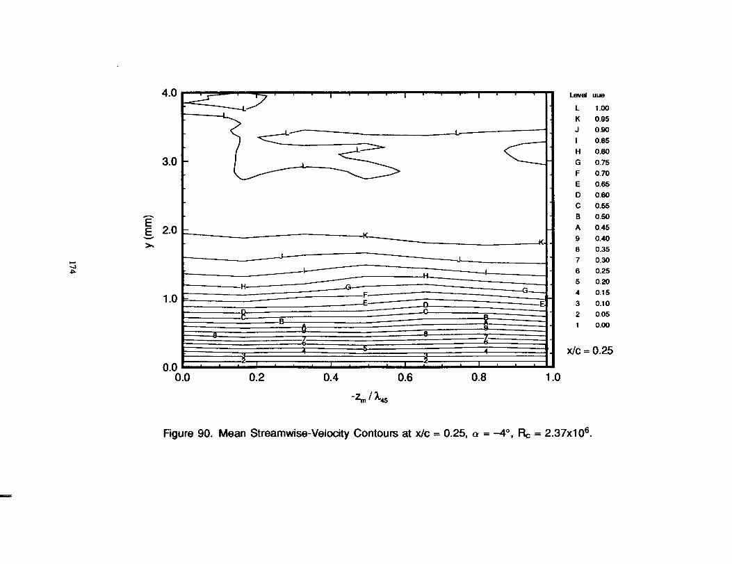
_0
00
00
00
00
00
00
00
00
00
0
(ww
)
o_1OII
ffEN
,LOOxO,III
o7_II
c_ilOt-O8o_Ec_I.,I-
174
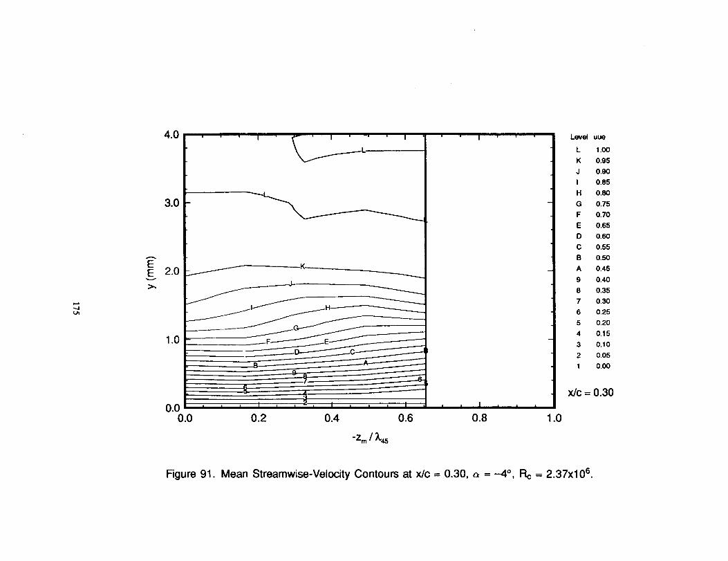
1
(ww
)
OcoO
EN
O
_OC3x03II
O7II
c_0_dII::3
OOo
!
8°_E(-O_::3
175
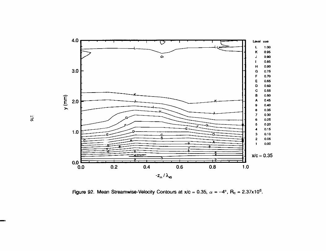
_00000000000000000000
o.o.
/o.
(ww
)
\\
u_0I1
E
CO0xb,.II
0"tII
u_dII
e-0o°_Ee-e,i
176

o_o
_o
_o_
o_o_
o_o_o_
o_o
__
00
00
00
00
00
O0
00
00
00
00
QdIIo
EN
_D0xII
0TII
dII_30°_Er-(I)
c_°_U.
177
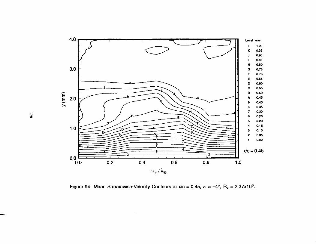
!_
00
00
00
00
00
00
00
00
00
00
:I,,|III
0
(ww
),_
II
E
_DxII
O7UdIIOO8I8°_EIT.
178

OII
E
_DQXC_c_II
n-oTII
c_0
II
g8
!8Ec_
c_
o_
LL
179
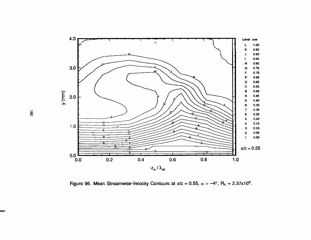
0_0_0_0_0_0_0_0_0_0_0
_0
00
00
00
00
00
00
00
00
00
00II
E
00
0xU0
n_0TIIIIc04_E_d°_LL
180
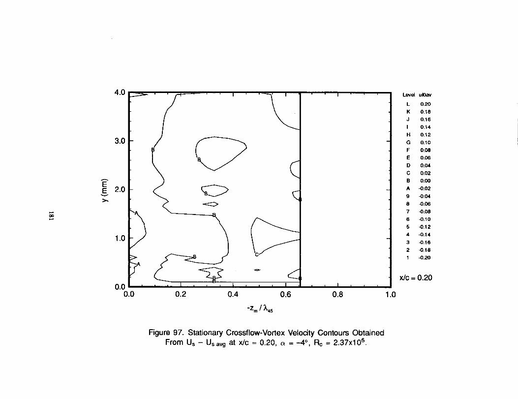
II
I
00II
l,
0
00000
AS
T- ,,o
''
''
,i
''
o--""
o.
o.
o.
04
',--
0
EN
7OO,--x
o_x,0IIO
i
0_E_,,
U.
181

182

-_II
0cO0000d00
0
E
x
o_*-II
000_E
183

ooooooooooo99_99_9o_
__
___
__
W_
__
__
__
__
__
__
(ww
},_
OII
E
_DO
_xO.II
X
QO
II
o'_5B
°EO,_,_O
='8.O
_c:
O
184

(ww
),_
QdII
E
N
_O
0.
r-X_ooII
°mo.o_c:
o
185

__--__O
m_m
_m__
J
\i
(ww
),_
dII
\\
E
_Do0_0
•
8_x
C_
0IIE
_u_C)
186
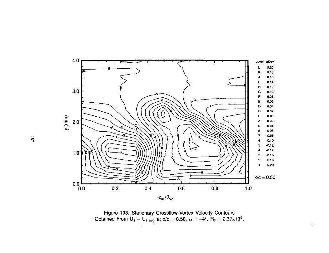
_ooddodddddd999_99_999
00II
0cO0_D000
E
_DQ
_xr_
:3co
o•
X
oo
II
cdE
o1.1_._0
o.o
o
(ww
),_
oo
oo
o
187
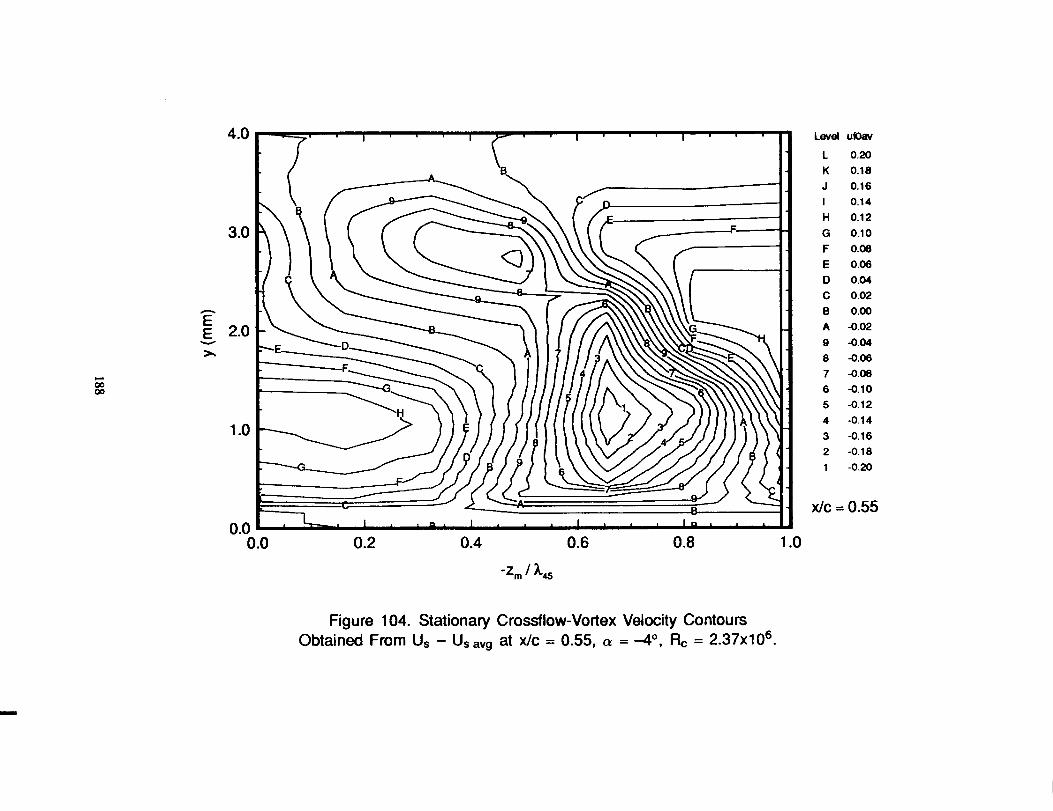
(ww
)
0II
0
0•
0II
_,n"
x°__E
0
188

(ww
),_
189
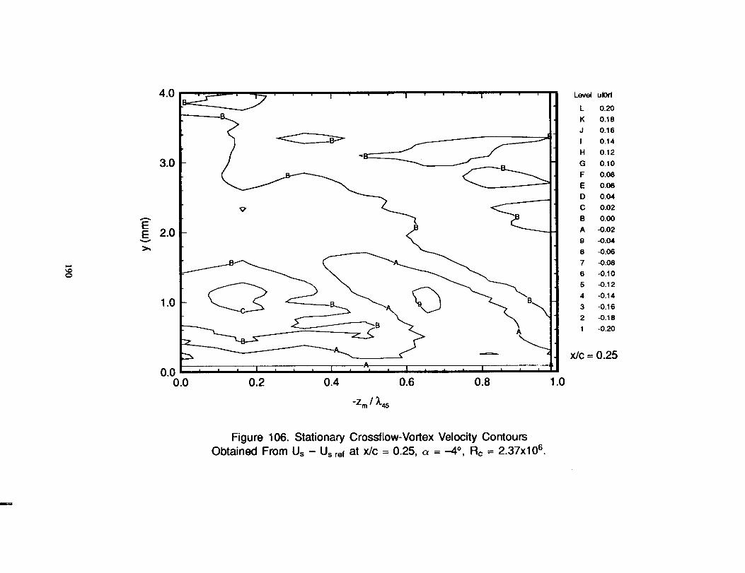
.....ooooooooo__
©
(ww
),_
0II
EN
r.D
_x0II
>..n"IIx0
II
o0_E
LI.
L_'_0
190
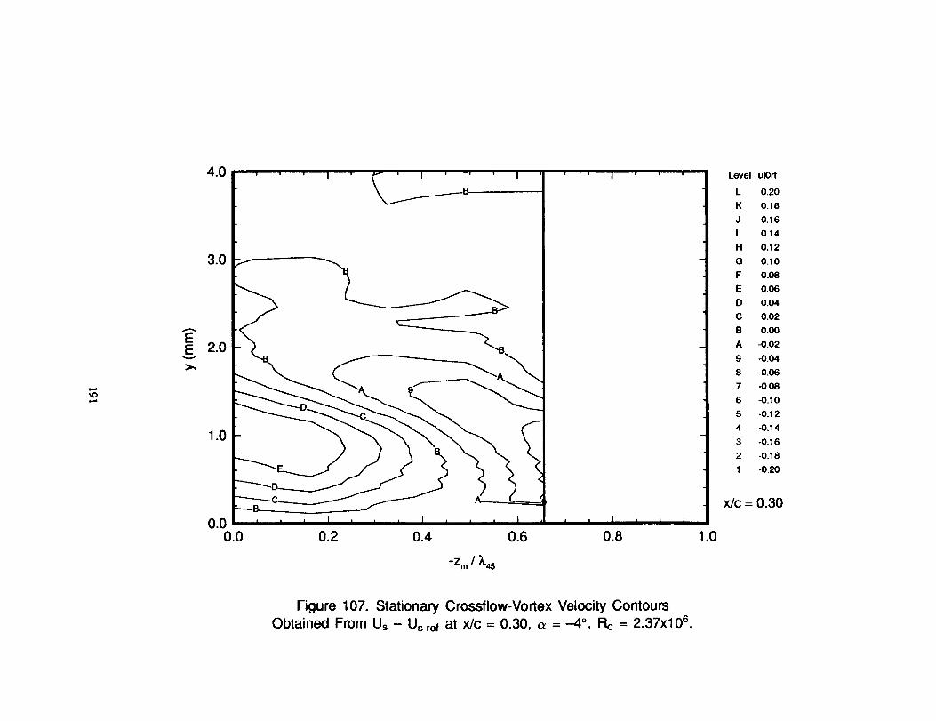
00000
E
00
0
_xITM
c-OII
0
IIx0
II
c_0_E
LL0
oo
oo.
0
0o
d
191
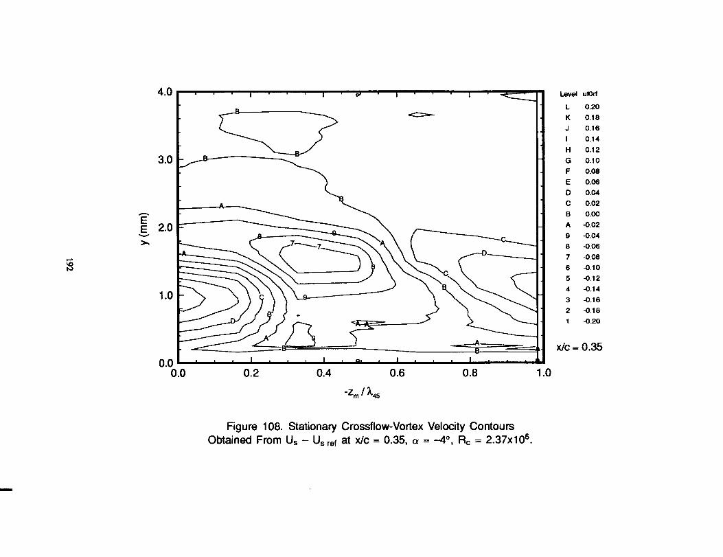
__
__
_0
00
00
00
00
__
__
__
_ddododooodo9999999999
/o.Q
oo.
(ww
)
0il
\
000
0
E
¢D0
0¢0
0II
0x0II
0_E
LI.
-,'8._0_
C:
L_'_o
192
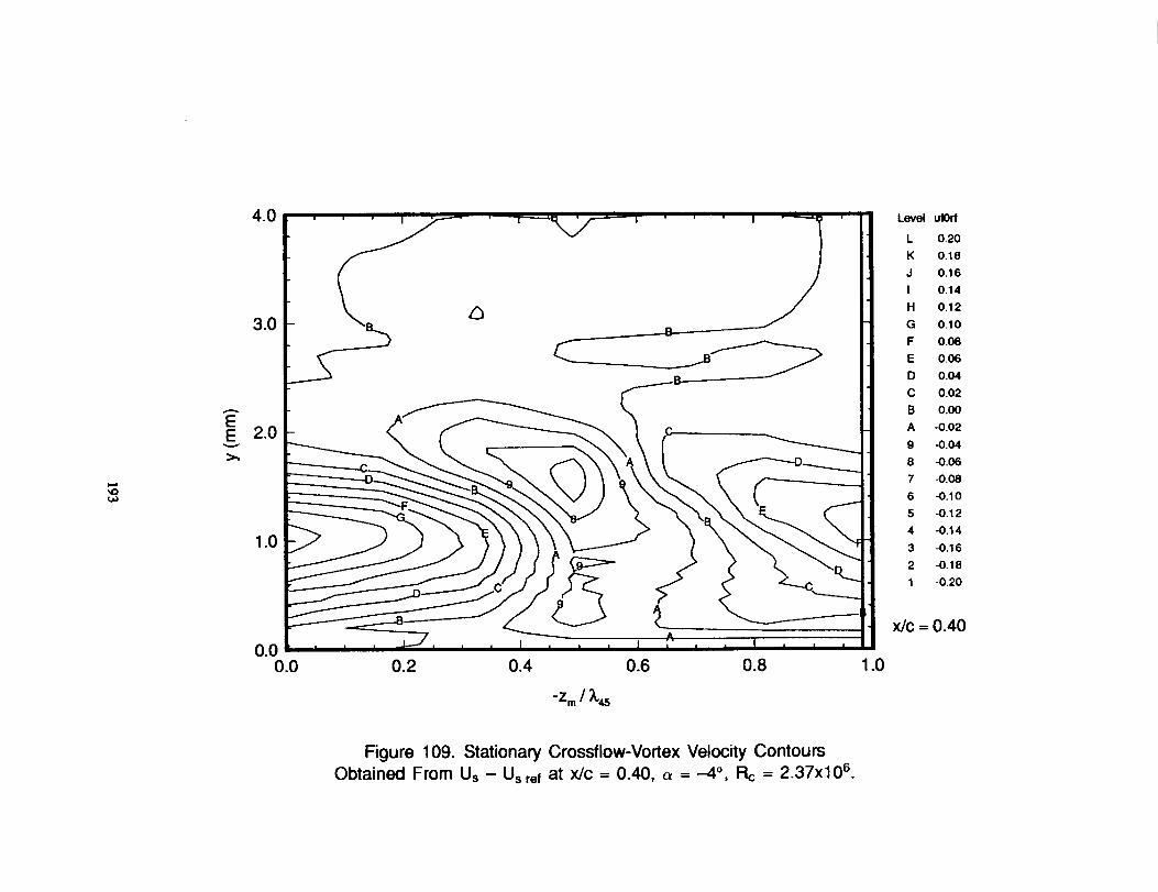
00U
E
0
_×0cO
0IIII
x._0II
0_E
U-
0
193
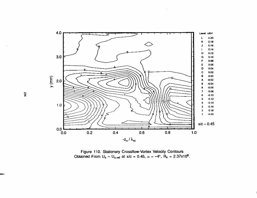
d11
ooo
E
(0o
o_
-'aic-O
IIoX_d._o
II
ooE1.1."_0
(ww
)
194
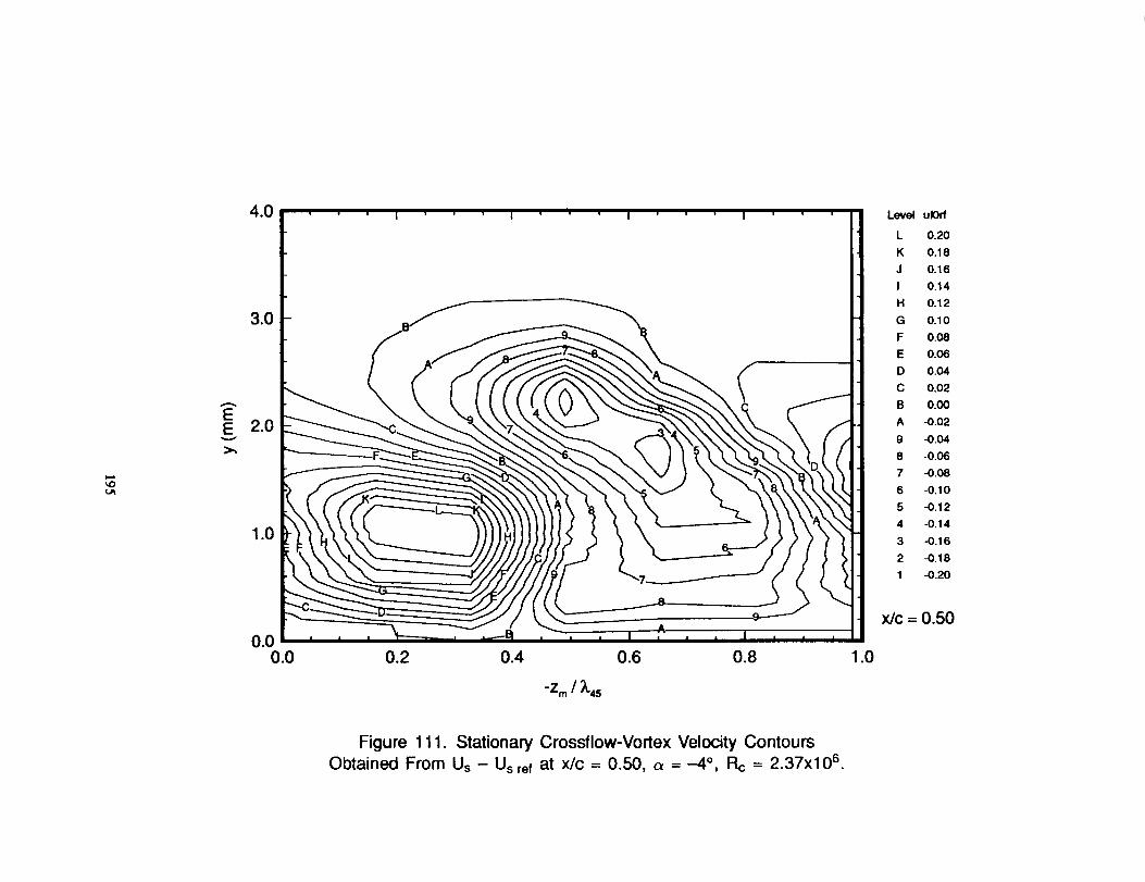
00li
000
EN
00
(.00
_x
(_0
II0
0IIx_m
_E=_0
oo
oq
(ww)
0
qC_
0
195

0II
00
E
0
_x0
II
ux__0
II
0,-.oL_
m.0_
r"
0
196

I!
....i
ii
ii
ii
iI
,°
,.,
I
oo.
oo
(ww
)_
00II
000
!
00
0,_,
0
0o
0
EN
0xII
o"tII
dII
P,E8°_I--°_U.
197

0!198
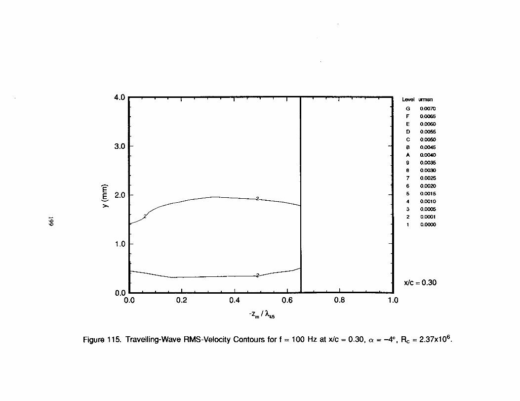
Iggg888888
.H
''
'i
....I
_Td
II
g0
,,
iI
._.
00
(ww
)_o_U
.
199

(ww
),_
0II
0cO00
c,oQxc_II
07II
0IIN7-00II00000::
°_I--L_
2OO

0
._0
00
00
00
00
00
00
00
0
_D
201
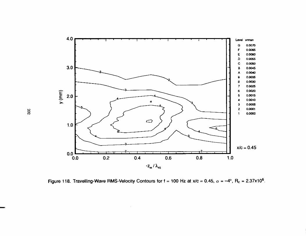
¢0
(ww
),_
.__U
-
202
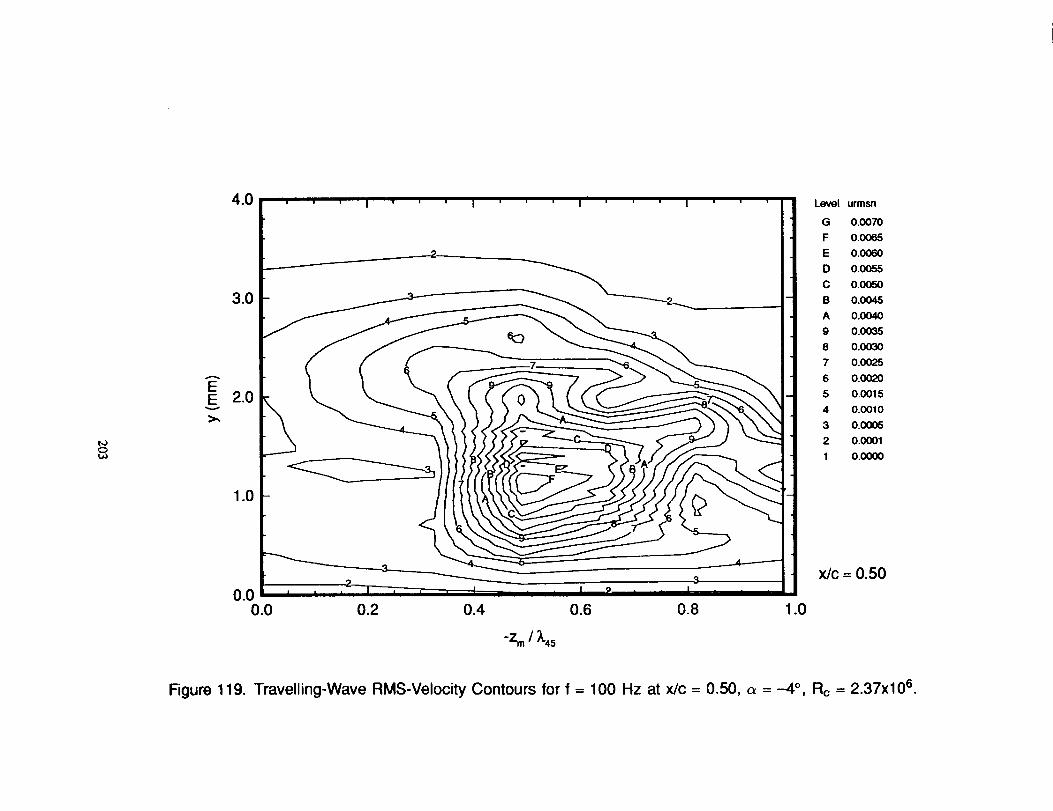
203

204

o
(ww
)
o¢.00xo3II
n"ou_!II0t-O0t--I-o3°_LI-
205
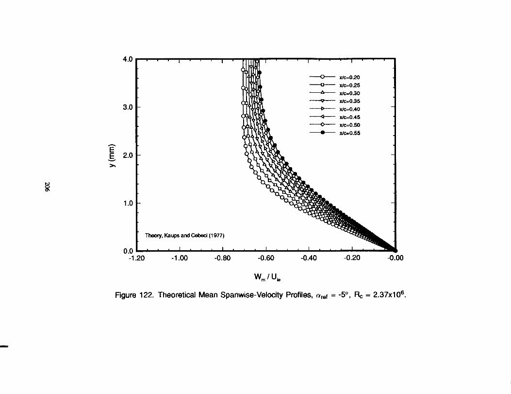
(ww
)
(D0XII
0
II
>(6c°_0I-

o
8
ooo
iE
O_
x
JOII
t'7o"
0o__E
°_o_
oo_
20"/
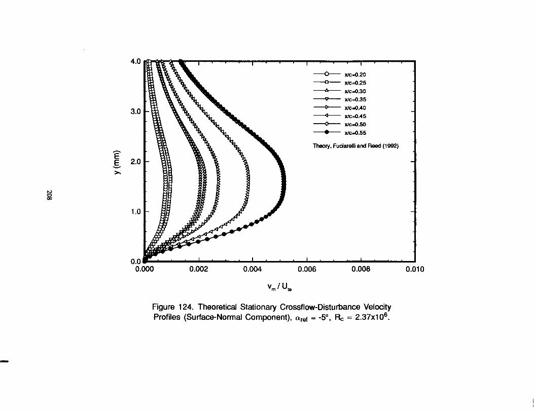
AvI
000CO
000000
°
0CII
0
208

''
'I
....I
''
'I
(_
O_e-
t-o
o
_'__
°_"e-
e'l
u,'im
,..-__
go
oo
ood
(ww
)
2O9

Im
,I
II
II
It
II
II
II
II
II
,q
q
(ww
)A
oo
¢Q,,-
•X
""r',-(-oeJII
on-
o0
II
ffl
E
dmC
o_1'._
d2oe-D
-
8_
210

Ii
t,tttt tt
|'
''
'I
A
ooJooocooo_0o0ooc_8
o.o.
o.o
o.oq"
CO
C_I
v-0
(ww
),_
_00xf,,.coII
oLO!II
4--,
O.0
m00¢0
q)
.e..a
m0(I)
r-
h-
Od-I
._m
U.
211

o
]'
(ww
)
o
D--
Q)
(,_0
•c
oQ
-2"!
o,,_or-
o._0
_.
oE0'1°_U
.
212
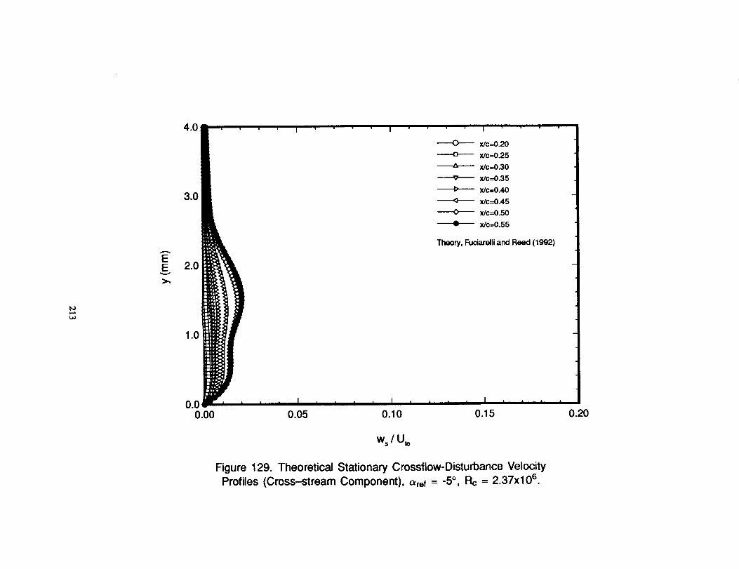
8
(ww
)
QOd
OO
XC_O
_o-rT_
0
.9E
_o
o__e_oU.
213

q
(ww
),_
o
0000ocO
ooooc_
o8oo
o
CDQxD,-
CO
C_H
OLO!II
xQ)
Q)
moa.8Q)
O¢)
p-
(:5
0_
U-
214
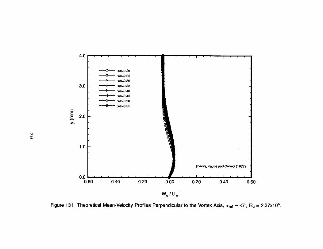
Ae"8.
I.-,-
°°,°°°°°
O
o.o.
o.o
o.o,
OX03c4Hoo
O
II
c_
X(1,)
O
O
o_
_t.
_)0.r.,O
o•
o,'_0,.
o,.q)
_mOt-l-eO
IJ_
215
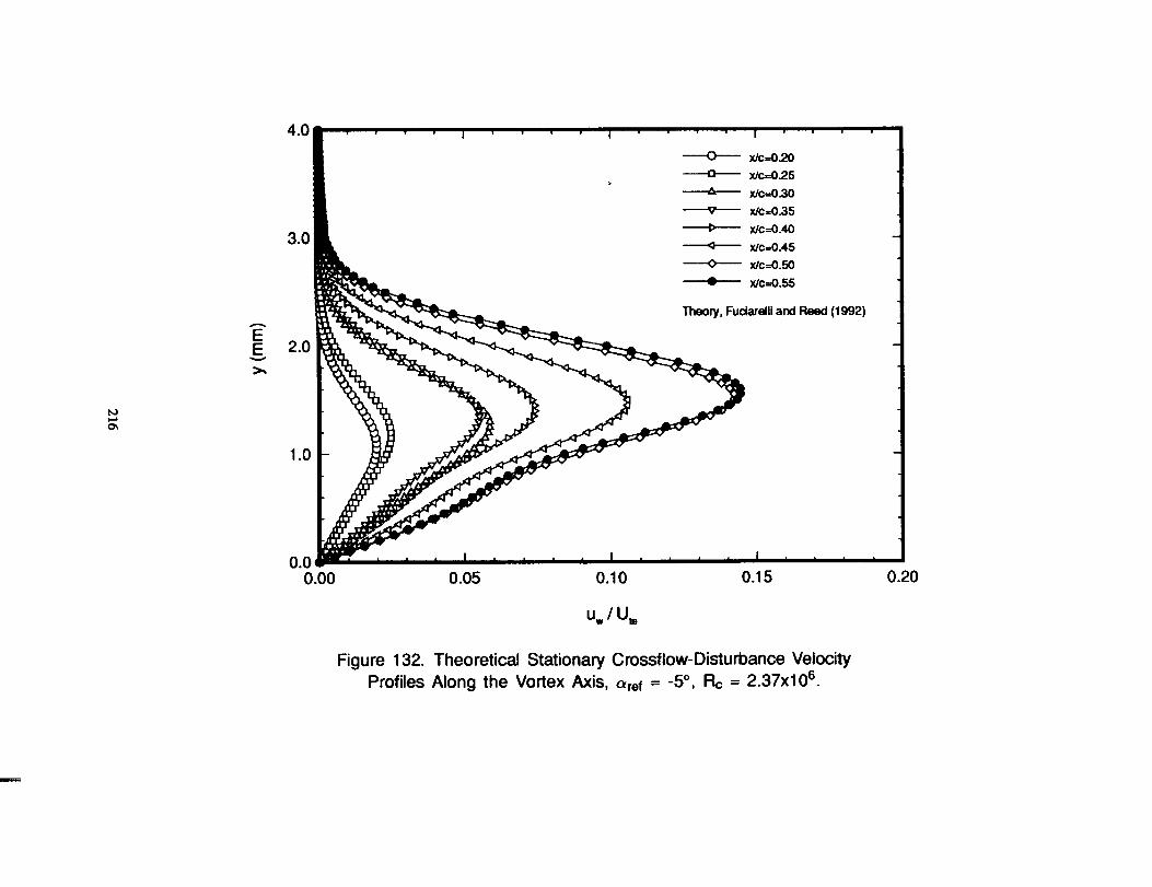
|•
''
'i
o0
00,
2.9xo
LL
216

,l
,i
j
v
_o_o_o_
l'
''
'i
'a
0,100
J
000
0II
_×
._o
-_o
00
r-
"_Q_
IJ-
_-
0.
217
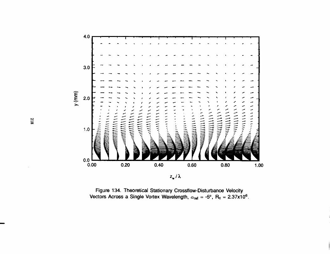
(ww
)
218

o0
o
t-
x
0"_o"-,m
,
0
,4">,_0
x_<_
E
a3o
_>•+-.+
,_
0e-l-
U>
(/),_o,-<_
_U.
219

lllls,-"220

q
00U
0II
I!
I
IA
E0c
oooooooo
Q
¢,00XC_
q)0_c_
O.
0xW
_-,,_I--0
._
o•
ED
0ot
M_
mE
iT'.=
_Ea
221

0II
0II
II
I
vJ1lILl
t-
O.
O.
O.
0
t_000'1'-ii
000008ooo
(ww
)
o
0'T"x14.
°_08_
_d•_u
•_.o
xW_-
I--
oE_
0oI
_E_-0
LL..EEr7
222
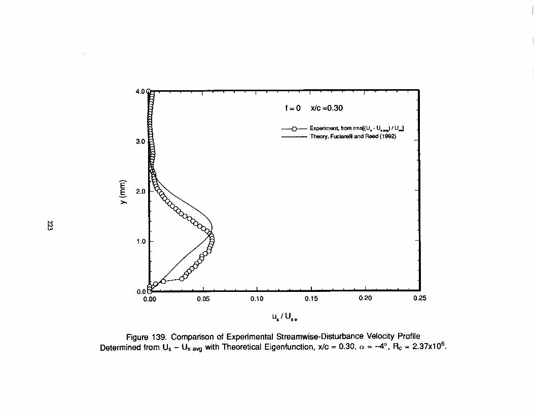
0C_
0II
0II
7A
¢im
II
oooooodg
(ww
)
0
0x
.o__o
ii
0_c_
-edE_
c
x_
Wc-
Oe-
-,-E_
01
0mE
_..__Ea
223

0U
0II
II
I
7
qo
(ww
)
ooooooooo
o.oo
0x
q)
c_"ec_
mc"
•_._o
•e-'_
X_
U.I
e-_.1"-0
e-
o_
ffl-_"
_I
m
E_
01
od_'_"Ee
_._E
224
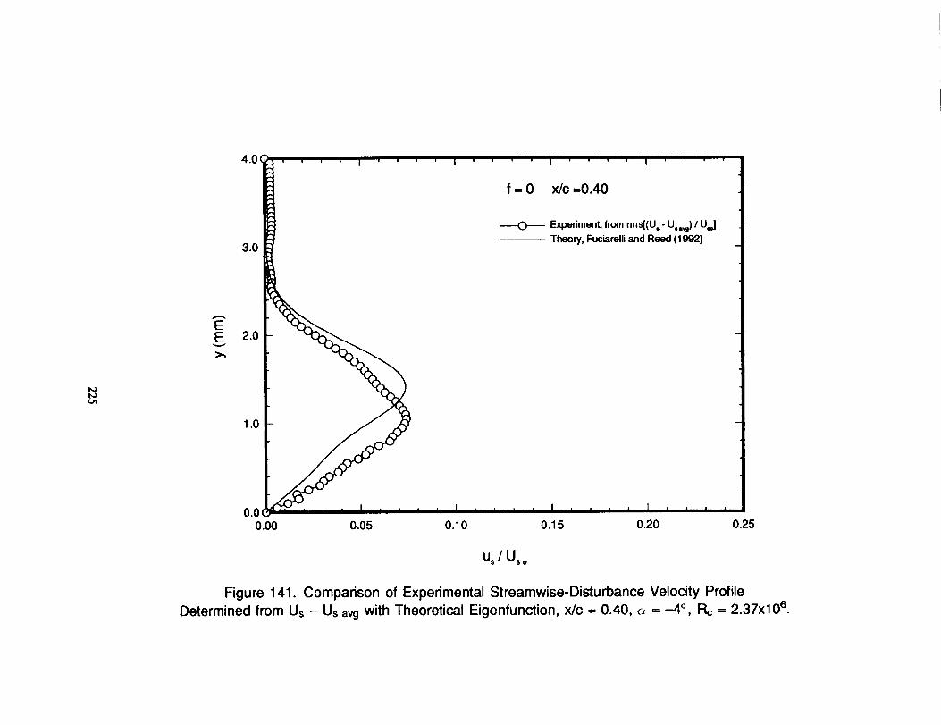
q,q-
odII
0
U
II
I
7A
-.._J
"-_8
'-_-ou.qo
o.
(ww
),_
u')
Qoou_ooou')oQ8
o
to0X14,,
q)
"ed
E_X
_W
c-
Oe-
l""°i
o_
ffl-r.-E
_o
I0
U')
.=)E
_..__
225
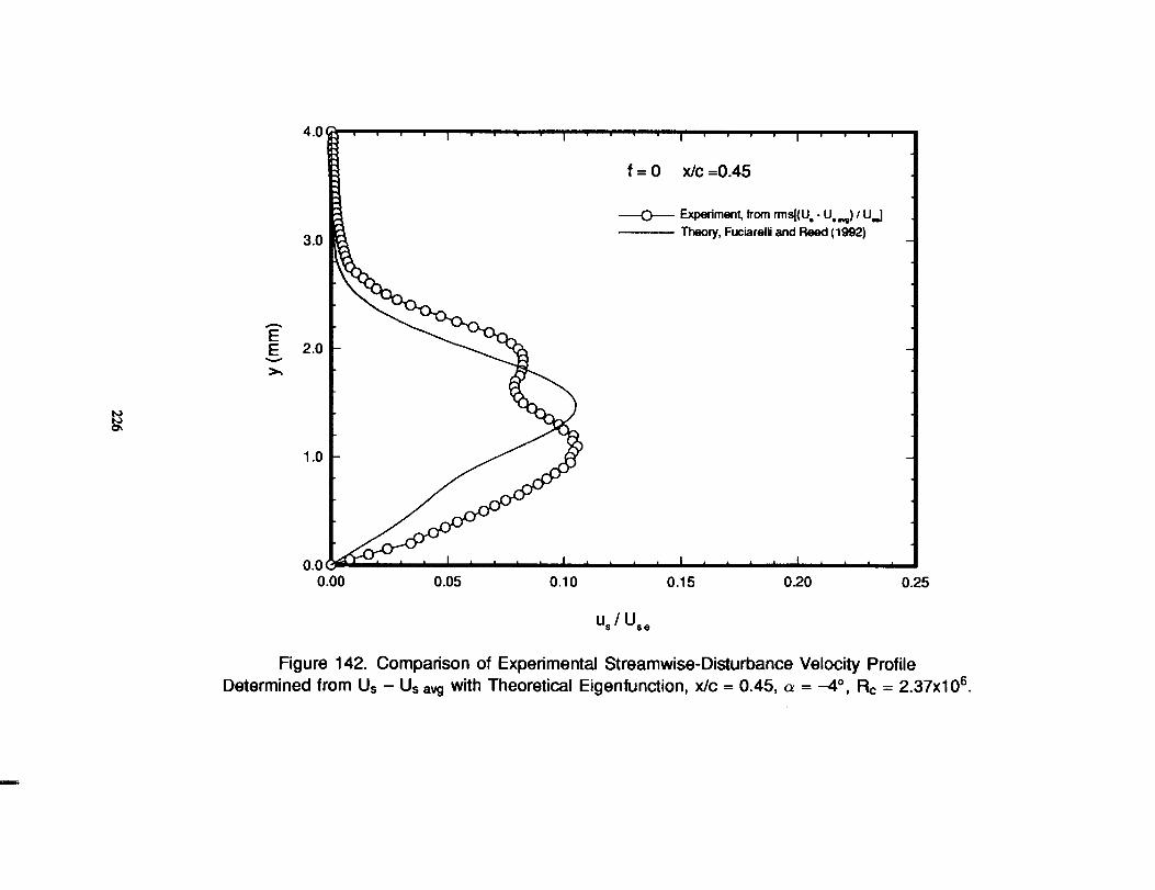
t,DotO
_>,
L_
__
"Li
_$_
(_
_.__d
Q
0,_E
EL_
r_
226

00II
oII
"lAv
i£)c_ooo
0X
0-Ed
Q)
"_
.9
E•r-4-,
O.
0XW
r-
-_-E_
oI
0
r_
227

(ww
)
o
0XII
a
22_
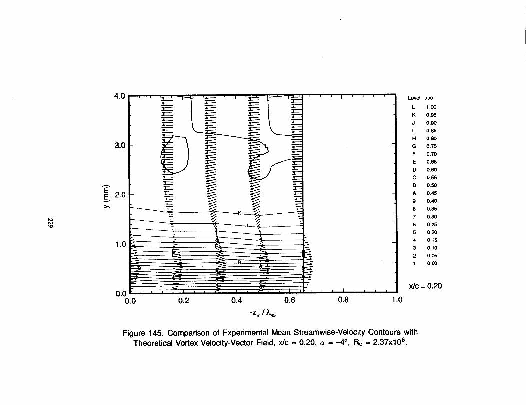
!....
II
''
0000
(ww
)
E
_ox
014.
o_u
-_c_
0
I
Ec_
_oe-o.>,
xW>"
o.90o>u)
•r-X
'_-0e-
:_1--.__ii
229
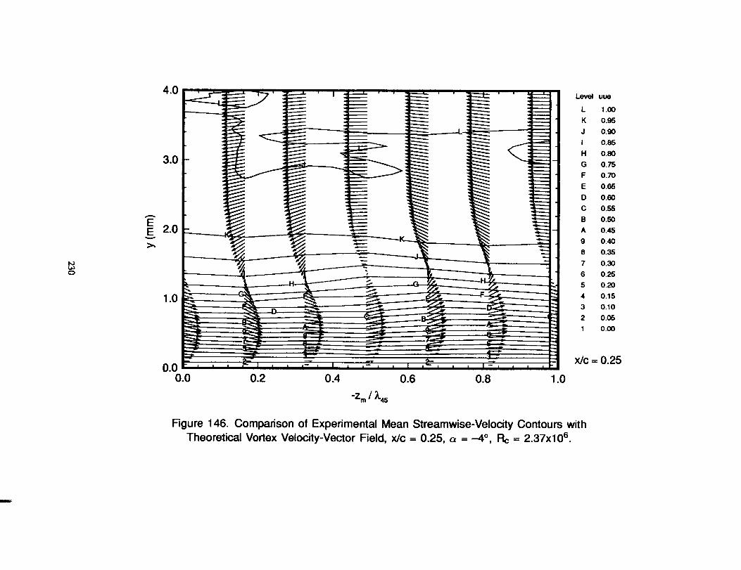
__
00
00
00
00
00
00
00
O0
00
00
(ww
),_
Lr)O
JdII
EN
0
¢-
_Ox0
14.
oo,i
!
0_II
°_O0
IILEoX
i
00
"C=
X
_I--.__I.I.
230

__dddddoo
doododddddood
Ii
i
0cO
0
II
0'T'--
cO
00
E
¢.,.
_o
x0o_
0II
•,-,
0
0
!(]3
°_
c_
f'_
II
(I)
_LK
x
.w0
00
"C
X
•-0
{3)
°_U.
231
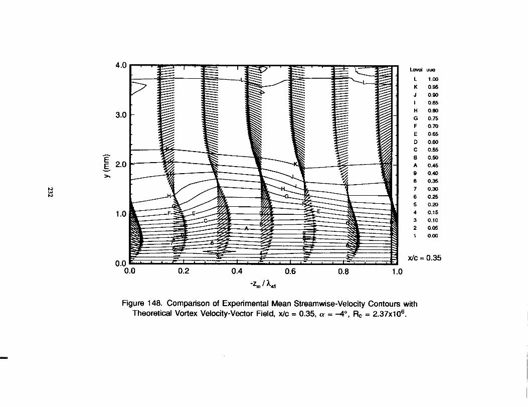
!_
00
00
00
00
00
00
00
00
00
00
!I
rllllIIIIlflrllflf Ilil///lllllllllllllllili_'"+'__
#lI
•°
l/l///lllllllllll////////_,_'I,\\\
(ww
)X
0II
00
E
0
q_
_o-_x
0cc_
o_i0
II
I:::_
.,..,o7D
"_i,E
Eo
Wo_
'*-0
00
•_X
0,r--0e-
.__Ii
232

__
00
00
00
00
00
00
00
00
00
00
.......
HIIJlfJIIJlllIIH
l JJll/ ___
VVVVVTTVYVYvvV
YTYTTYYYYY
//
/I
/(ww
)
00lii-
x0
f_.
o_0
ii
0!Ec_
f_II
•"-0
00
CLI_
0"_•.¢,_
O_
_'
""0e-
--sI-.
.__U.
233
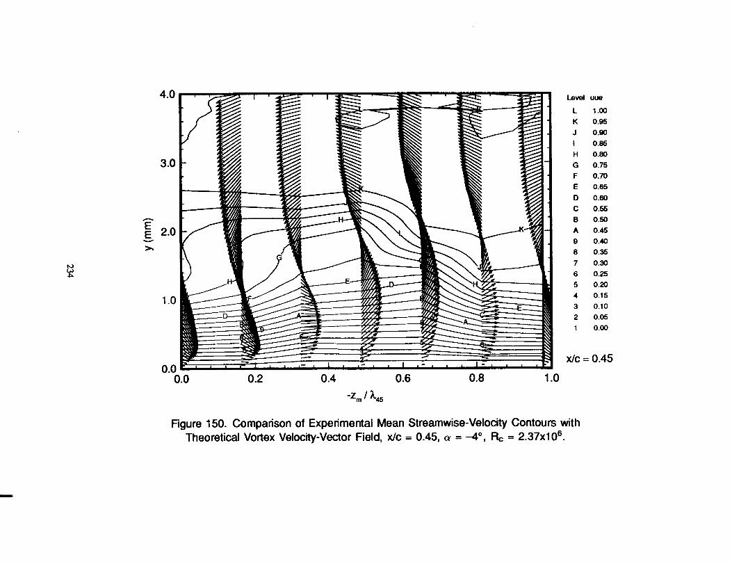
0
0!
(0II
°m
00
0
234
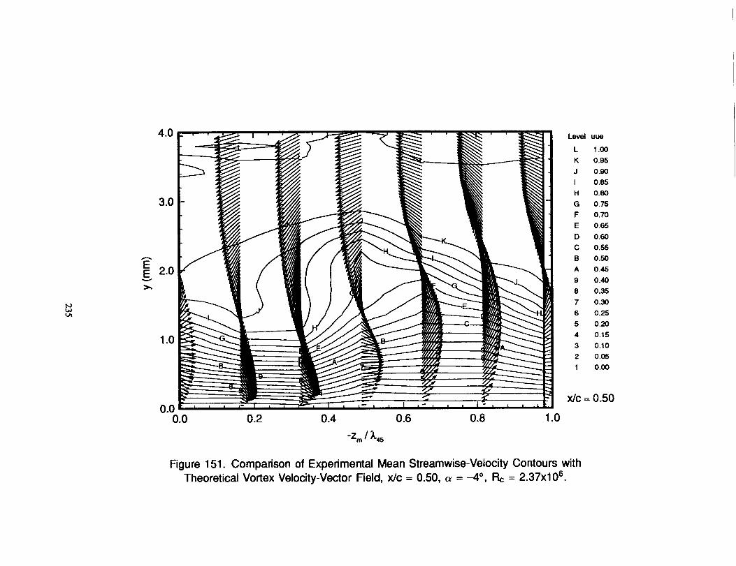
__d
ddddddddddddddddddd//
///1
(ww
)
235
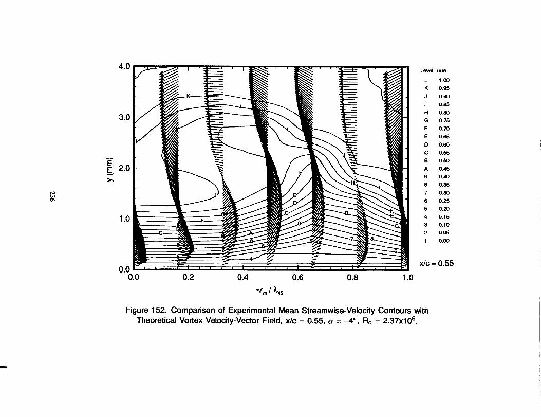
i
(ww
)
0
0
236

ooooooddddd9999999999
II
I
(ww
),_
OOII
OaOO
EN
-IOO_
OO
x03
Oo0_
ou!
m_
E"_"
"8
XW×
_u
•,-"_
_°_
00
_me-
.I--
U.
237
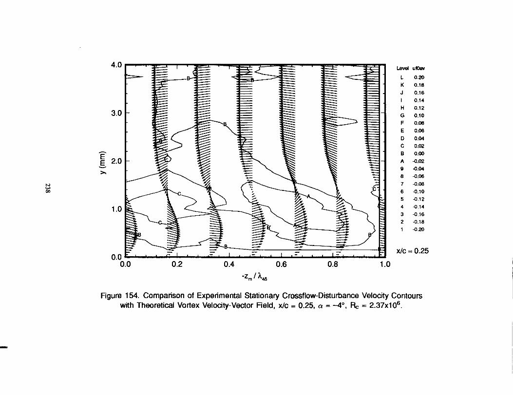
oc2.
oo
lDOJ
dtl
OcOO_DO
E
OOd
OO
Oo
O
O°
O_
Oo
x
Oo3
°c_q)r-
r7
II!m
_
•r-O
•m
XUJ
×
0Or-
LOt-
O)
LI.
238

0cOC3
00
0
(ww
)
0c-Oco
Oo
x
0o_ode-
o¢0_de
tt
"_-0
q)a
XW×
,4-
0%:
m
00
I.'3
U_
.c
U.
239

240

..I
__00__
ooooooooooo_99_o99_9
o.o.
o.o
00II
=
'tt,°
II,°
0oO0¢q00
0
0¢-
C)
0x14,.
¢Dt-
eT_=3_d
!
E""0
"¢-o
Wx
,_-¢_
(J_m
•.0_
00
0_t'-
mr-
_°_
IF.
241
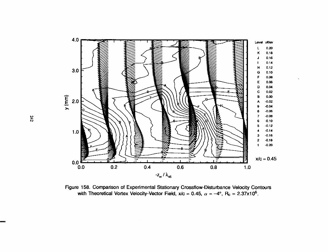
0II
242

oo.
00II
243
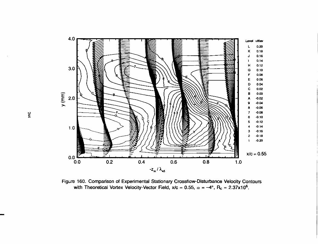
oo
qo
•_-
0")
oJ
_-
(ww
),_
u')
0II
0
0O©
Oo_,
x•'='-
r,-.o,..o_
c:
eTo
_Jl
o_a_
_m
o_•e-
"_m
_o
xU.I
x
01=
_o
0o
0
a
00
0mr.-
._--
o_D
r-
°_
U..
244

I'
'"
I'
'I
"'
'I
"'
I
0
0QC_J
0
....
I,
,,
,I
,,
,,
I....
I....
I....
00
00
00
00
00
00
00
00
00
00
0
0X
c-
O
X
X"0
U
Q_
0x
._.-
E,
o0o
._0
o/'_
2.,45

__oE
iI
_L
LI
O"OC
II
O
_e--
e-
o_o,9oO
OO
D
OO
_.o
o_O
o
°_
246
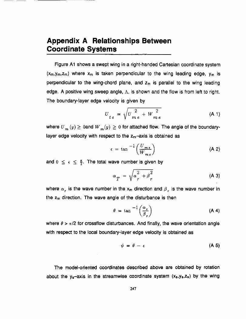
Appendix A Relationships BetweenCoordinate Systems
Figure A1 shows a swept wing in a right-handed Cartesian coordinate system
(xm,Ym,Zm) where Xm is taken perpendicular to the wing leading edge, Ym is
perpendicular to the wing-chord plane, and Zm is parallel to the wing leading
edge. A positive wing sweep angle, A, is shown and the flow is from left to right.
The boundary-layer edge velocity is given by
iU 2 2= + W (A1)Ute me me
,,, (y) > 0 for attached flow. The angle of the boundary-where U,,, (y) > 0and W
layer edge velocity with respect to the Zm---axis is obtained as
= tan \Wm_
and 0 < e < _-. The total wave number is given by
la2 f12a T = +r v
is the wave number in the Xm direction and #_where o_
the Zm direction,The wave angle of the disturbanceisthen
8 : tan-l(a_-)
(A 2)
(A 3)
is the wave number in
(A 4)
where 9 > _-/2 for crossflow disturbances. And finally, the wave orientation angle
with respect to the local boundary-layer edge velocity is obtained as
¢ = 0 - e (A 5)
The model-oriented coordinates described above are obtained by rotation
about the ys-axis in the streamwise coordinate system (xs,ys,zs) by the wing
247
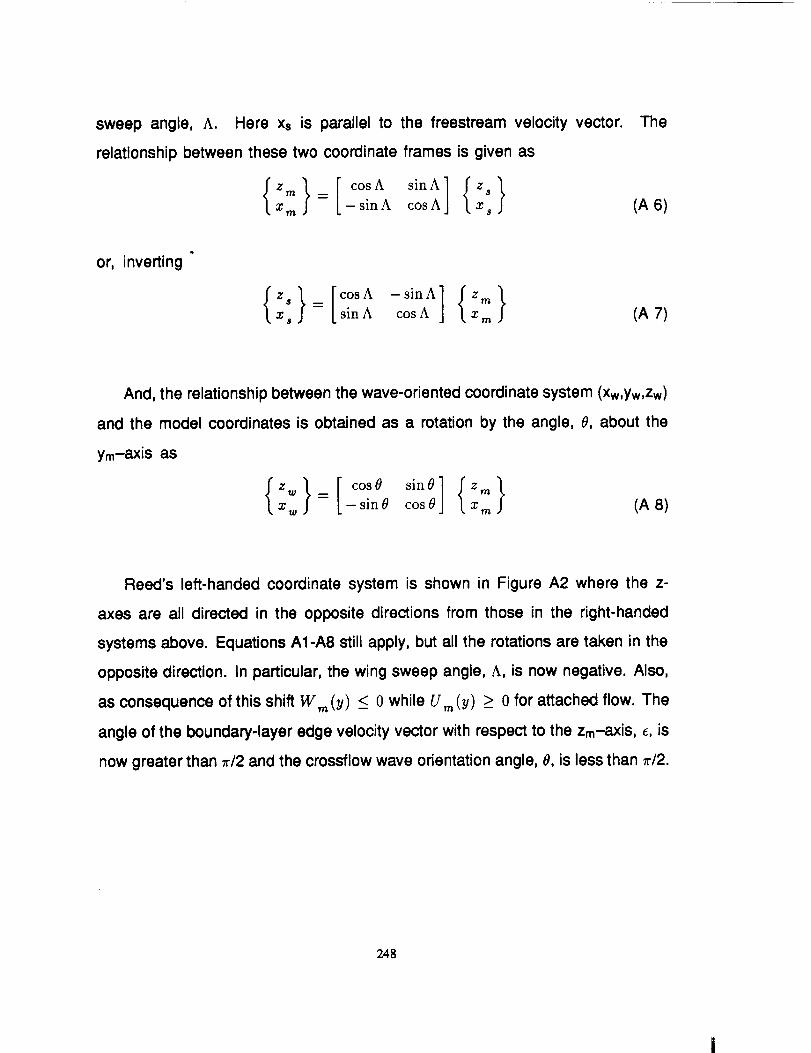
sweep angle, A. Here xs is parallel to the freestream velocity vector. The
relationship between these two coordinate frames is given as
xm -sinA cosA xs (A6)
or, inverting
_sio ]{z.}x_ = sinA cosA x.., (A 7)
And, the relationship between the wave-oriented coordinate system (xw,Yw,Zw)
and the model coordinates is obtained as a rotation by the angle, O, about the
ym-axis as
x,.v = - sin 8 cos 0 x _ (A 8)
Reed's left-handed coordinate system is shown in Figure A2 where the z-
axes are all directed in the opposite directions from those in the right-handed
systems above. Equations A1-A8 still apply, but all the rotations are taken in the
opposite direction. In particular, the wing sweep angle, A, is now negative. Also,
as consequence of this shift W,.,,(y) < 0 while U,,(y) > 0 for attached flow. The
angle of the boundary-layer edge velocity vector with respect to the zm-axis, e, is
now greater than _-/2 and the crossflow wave orientation angle, 8, is less than _-/2.
248

oc_t-c_
<&
249
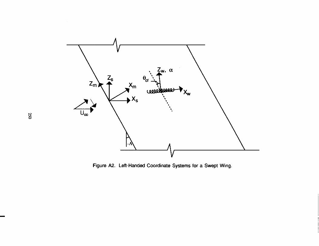
t_t,-.
o.-I
250

Appendix B Hot-Wire SignalInterpretation Procedure
The freestream and boundary-layer velocity measurements are performed
using Dantec 55M01 constant-temperature anemometers equipped with 55M10
CTA standard bridges with bridge resistance ratios of 1:20. The hot-wires are
Dantectype 55P15 miniature boundary-layer probes having 5-/_m platinum-plated
tungsten wires which are 1.25 mm in length. The probe tines are 8 mm long and
are offset 3 mm from the probe axis. Standard 4-mm diameter probe supports
are used. The three-dimensional traverse system (described in Chapter 3) is used
to support and move the probes through the flow field. The traverse system is
mounted external to the test section with only the probe-support sting extending
through a sliding opening in the test-section wall. The sting consists of a composite
element and an aluminum strut. The composite element is 5 mm thick, 0.425 m
long, and its chord tapers from 64 mm at the base to 50 mm at the tip. The
aluminum strut dimensions are 13 mm x 76 mm x 0.324 m. Both the steady-state
and fluctuating hot-wire signals are sampled simultaneously using the 16-channel
MASSCOMP 12-bit A/D converter which can sample at an aggregate rate of up
to 1 MHz. The fluctuating voltage signal is narrow band-pass filtered using a
Spectral Dynamics SD122 equipped with a 4--pole Butterworth tracking filter with
+10 Hz passband.
The voltage response of a constant-temperature hot-wire anemometer can be
assumed to have the form
E = F(p,v, r0) (B1)
where p is the ambient air density, U is the velocity, To is the total temperature,
and E is the anemometer voltage response. Differentiating Equation B1 givesdF dF dF
dE = -_p dp + -_ dU + "_o dT 0 (B 2)
251

Thus, a small voltage change is dependent on small changes in the density,
velocity, and total temperature.
It is desirable to reduce the complexity of the functional relationship given
in Equation BI. This can be accomplished by eliminating or at least minimizing
the variations in p and To so that the anemometer response depends solely on
the velocity. The UWT has no heat exchanger system to maintain a desired
tunnel temperature. The tunnel total temperature increases with test time until an
equilibrium condition is achieved. For the present experiment the tunnel flow is
preheated by operating the tunnel at the expected test condition for 45 minutes to
1 hour before hot-wire probe calibration. This provides sufficient time for the flow
temperature to reach its equilibrium value. The air density depends on two factors
-- atmospheric pressure and flow temperature. To minimize atmospheric pressure
effects the hot-wire calibrations are conducted before each data-acquisition run.
These steps insure that dp and dTo are nearly zero and can be neglected in
Equation B2. Then, Equation B1 can be simplified to
E = f(U) (B 3)
The hot-wire probes are calibrated in the UW'I" flow by varying the freestream
velocity in steps across the range of velocities expected during the experiment.
Typically twelve velocities are used for each calibration. Equation B3 is not actually
used for probe calibration; instead,
U = g(E) (B 4)
is used where g(E) is a fourth-order least-squares curve fit to the calibration data.
Then, f(U) is determined as
-1E = .f(U) = g (S) (B 5)
252
Differentiating Equation B3 gives
df !
dE= _ dU= f dU (B6)
Now we assume that
/e =E+e (B 7)
andI
u = U+u (B 8)
where e is made up of a steady (or DC) voltage, E, and a small fluctuating voltage,I I
e and u consists of a steady velocity, U, and a small fluctuating velocity, u.
Substituting Equations B7 and B8 into Equation B3 and expanding in a Taylor
series while neglecting higher order terms (since e_ and u t are assumed to be
small) we obtain
' ( ) =S(U)+S !(U) u (B9)E+e =S U+ ul t
Subtracting Equation B3 from Equation B9 yields
= S !(U) .! (S 10)
or solving for u I we obtainI
/ eu - (B 11)
f'(u)
Since u _ and e I are small deviations from the steady values of U and E, we
can apply Equation Bll not just at a single point in time but for ul(t) and el(t)
as functions of time while holding fl(u) constant and then take the root mean
square of these functions to getI
/ e (B 12)U rrns
253
which gives the rms velocity fluctuations as a function of the measured rms voltage
output from the hot-wire anemometer circuit.
For boundary-layer velocity-profile measurements we desire the ratio of local
velocity to the boundary-layer edge velocity. Two hot-wire probes are used for
this measurement B one probe located in the boundary layer and the other in
the external flow. Both probes are mounted on the traverse strut and moved
together as the boundary-layer velocity profile is measured. The probe in the
external flow is not located at the edge of the boundary layer but is, in fact,
located approximately fifteen centimeters from the boundary-layer probe. During
the traverse the two hot-wire probes move only about 4 mm. Over this distance
the external flow probe detects only negligible variations in the velocity, but the
boundary-layer probe sees the velocity decrease from the edge value down to
near zero as the surface is approached. The boundary-layer velocity ratio cannot
be obtained directly as the ratio
U2
U1because U1 is not at the boundary-layer edge. However, the desired velocity ratio
is given by
where
(B 13)
U
U3e
is the boundary-layer velocity ratio, U1 is the external flow velocity, and U2 is the
boundary-layer velocity. By scaling the measured velocity ratio,
U_U1
in Equation B13 by the velocity ratio observed at the maximum distance from the
surface we normalize the profile to unity at the boundary-layer edge. This accounts
for the fact that the external-flow hot-wire probe is not at the boundary-layer edge.
254

Appendix C Error Analysis
Kline and McClintock (1953) discuss the effects of experimental measurement
errors on computed data in various experimental situations. They discuss both
single- and multiple-sample experiments, but their primary emphasis is on describ-
ing uncertainties in single-sample experiments. For multiple-sample experiments
statistical methods can be used to establish both the mean values and variations
from the mean. However, in single-sample experiments errors in the results com-
puted from experimentally measured quantities can only be estimated. Kline and
McClintock show that the uncertainty, w R, for the computed result
R = R(Vl'V2'v3'""vn)
can be obtained as
= w iW R i=l
(C 1)
(C 2)
where v_ are the measured quantities used in the computation of R and w, are
the expected error ranges for the measured quantities.
In the present experiment the range of measured quantities is limited to static
and dynamic pressures, pressure differentials, flow temperature, and hot-wire
anemometer voltages. From these measured quantities the freestream velocity,
the surface pressure coefficients, boundary-layer and edge velocities, and, most
importantly, the boundary-layer velocity ratios are determined. The freestream
velocity can be obtained from the incompressible Bernoulli equation and the
perfect-gas equation of state as
U = _/2 qoo RT_ (C 3)
oo V Poo
where Uoo isthe freestreamvelocityand the measured quantitiesare the dynamic
pressure,qoo,the staticpressure,Poe, and the statictemperature,Too, while R
255

is the gas constant from the equation of state. The surface pressure coefficient
is given by
C = p-p°° = P._.o.o (C4)P q_ q¢¢
where Cp is the pressure coefficient and p is the local surface pressure. The
boundary-layer and edge velocities are obtained from the hot-wire calibration
functions
U = g(E) (C 5)
while f (U) = .q-1 (E) is the inverse of the hot-wire calibration function.
Equation C2 can be applied to the Eq. C3-C5 to obtain uncertainty estimates
for U_o, Cp , and U as
Wc. d(w,o _ 2 (w,. _2C, - Vt--_Di + \-'_-_ / (C 7)
and
(C 8)
Equations C6 and C7 can be straightforwardly applied because estimates
of the uncertainties involved are easily obtained. However, Equation C8 is
much more difficult to apply since an estimate of the uncertainty in the hot-wire
anemometer voltage is much more difficult to ascertain. This difficulty can be
overcome by recognizing that in the present experiment some of the hot-wire
measurements can be considered as multiple-sample measurements while other
measurements must be regarded as single-sample measurements.
256
The most importanthot-wiremeasurements involvedeterminingthe boundary-
layervelocityratiogiven in Equation A12 as
where U2 isthe velocityindicatedby the hot-wireprobe insidethe boundary layer
and UI isthe velocityindicatedinthe outer flow, U2 and
U2
UI
must be regarded as single-samplemeasurements even though UI and U2 are
evaluatedas time averages ofrepeated measurements taken at a frequency offs
= I kHz over a 30 second interval,On the other hand, UI and
can be regarded as multiple-sample measurements and analyzed statistically
since these two variables are measured repeatedly during a hot-wire survey of
the boundary layer.
According to the instrument handbook the uncertainty in the measurement of
qc_ and p_ in Equation C6 is 0.08% of reading, but qc_ is observed to oscillate
due to a very low-frequency modulation of the fan controller at about 1% of reading.
Thus, the expected uncertainties for qo_ and poo are taken as
w = 0.02 torr at q = 2.00 torrqoo oo
and
w = 0.6torr at p = 720.0torrPoo <_
Also, the thermocouple is found to be in error by
WTo ° =-1.5°K atT = 309.0° K
oo
257
Substituting these uncertainties into Equation C6 gives
w u¢o= 0.6%
Uoo
If the uncertainty in Cp is evaluated at the maximum pressure point, then sub-
stituting
w = 0.02tort at PD = qoo = 2.00tortPD
into Equation C7 yields
The uncertainties in U_ and
are evaluated statistically at each fractional chord measurement station. The
standard deviation for U1 is found to be between 1% and 3% of Us • for all of
the measurement locations except x/c = 0.55 where it reached 5.56%. But, more
importantly, the standard deviation in the velocity ratio is much smaller ranging
from 0.15% to 1.38%.
An alternate method to estimate the error in the boundary-layer velocity ratio
can be dedved by using King's law as the calibration function for a constant-
temperature hot wire
E 2 = A+BU n (C 10)
where we take n = 1/2. Or, solving for U
U = E (C 11)
Strictly speaking, the calibration coefficients depend on the temperatures of the
hot wire (Tw) and the flow (TI) as
A = AI(Tw-Tf) (C12)
258
and
B= BI (Tw-T f ) (O13)
Now, suppose that the flow temperature changes from the calibration temperature
giving,
and
Ac(T _ - Tf)A = (C 14)
B = c (c 15)(r -rc)
where A c and B c are the values of A and B determined at the calibration
temperature (To). Substituting Equations C14 and C15 into Cll for hot wires
1 and 2, and taking the ratio _ we obtain
But, if Tf = T c Equation C16 reduces to
( ) E2U2 ½ Bc1 2 - Ac2 (C 17)-- 2
Be2 E 1 - Acl
An estimate of the error in _ is obtained by taking the ratio of Equations C16
and C17 and squaring the result. Doing so for a typical set of hot-wire calibration
data with the maximum temperature shift taken to be Tf - T_ = 4° 0 we find
that the effect of temperature drift is negligible at the boundary-layer edge, but it
increases as U2 is decreased. For most of the boundary layer, 0.25 < ._, < 1.0
the error does not exceed 2.7%. The maximum error is 5.8% at the minimum
velocity ratio of _ = 0.10
259
References
Arnal, D. 1989 Some transition problems in three-dimensional flows. In Instabilityand Transition: Proceedings of the ICASE / NASA LaRC Workshop. NewYork, Springer-Verlag, 1990.
Arnal, D. and Aupoix, B. 1992 Hypersonic boundary layers: Transition and turbu-lence effects. In ESA, Aerothermodynamics for Space Vehicles, pp. 25-38.
Arnal, D., Casalis, G., and Juillen, J. C. 1990 Experimental and theoretical analysisof natural transition on 'infinite' swept wing. In Laminar-Turbulent Transition:Proceedings of the IUTAM Symposium, Toulouse, France, Sept. 11-15,1989. Berlin and New York, Springer-Verlag, 1990.
Arnal, D. and Coustols, E. 1984 Application de crit_res bi et tridimensionnels aucalcul de la transition et de la couche limite d'ailes en fl_che. AGARD CPNo. 365, Paper No. 12.
Arnal, D., Coustols, E., and Jelliti, M. 1985 Transition en tridimensionnel etlaminarisation de la couche limite sur une aile en fl_che. Colloq. A_rodyn.AppL 22nd, Lille, France.
Arnal, D., Coustols, E., and Juillen, J. C. 1984 Experimental and theoretical studyof transition phenomena on an infinite swept wing. Rech. A_rosp. No. 1984-4.
Arnal, D., Habiballah, M., and Coustols, E. 1984 Th_orie de I'instabilit_ laminaireet crit_res de transition en _coulement bi- et tridimensionnel. R_ch. A_rosp.No. 1984-2.
Arnal, D. and Juiilen, J. C. 1987 Three-dimensional transition studies at ON-ERA/CERT. AIAA Paper No. 87-1335.
Arnal, D., Juillen, J. C., and Casalis, G. 1991 The effects of wall suction on laminar-turbulent transition in three-dimensional flow. In Boundary Layer Stability andTransition to Turbulence, ASME FED-VoL 114.
Bacon, J. W. Jr., Tucker, V. L., and Pfenninger, W. 1959 Experiments on a 30 °12 per cent thick symmetrical laminar suction wing in the 5-ft x 7-ft Universityof Michigan tunnel. Northrop Rep. NOR-59-328 (BLC-119).
PREf_EDii',_G PAGE BLANK NOT FILMED261
_.._jiimUmlMMa _.
Balakumar, P. and Reed, H. L. 1991 Stability of three-dimensional supersonicboundary layers. Phys. Fluids A 3: 617-632.
Berry, S. A., Dagenhart, J. R., Brooks, C. W. Jr., and Harris, C. D. 1990 Boundary-layer stability analysis of Langley Research Center 8-foot LFC experimentaldata. In Research in Natural Laminar Flow and Laminar Flow Control NASA,
Langley Res. Ctr., Hampton, VA.
Berry, S. A., Dagenhart, J. R., Viken, J. K., and Yeaton, R. B. 1987 Boundary-layer stability analysis of NLF and LFC experimental data at subsonic andtransonic speeds. SAE Paper No. 87-1859.
Bassom, A. and Hall, P. 1990a On the interaction of stationary crossflow vorticesand Tollmien-Schlichting waves in the boundary layer on a rotating disk.NASA CR-181859.
Bassom, A. and Hall, P. 1990b Concerning the interaction of non-stationary cross-flow vortices in a three-dimensional boundary layer. NASA CR-182037.
Bassom, A. and Hall, P. 1990c Vortex instabilities in 3D boundary layers: Therelationship between GSrtler and crossflow vortices. NASA CR-187456.
Bassom, A. and Hall, P. 1991 Vortex instabilities in three-dimensional boundarylayers - The relationship between GSrtler and crossflow vortices. J. FluidMech. 232: 647-680.
Bieler, H. and Redeker, G. 1990 Entwicklung von transitionskriterien auf e sup nbasis fuer dreidimensionale fluegelgrenzschichten (Development of transitioncriteria on the basis of e to the n power for three-dimensional wing boundarylayers). In DGLR, Flows with Separation, pp. 103-116, Bonn, F. R. Germany.
Bippes, H. 1989 Instability features appearing on swept wing configurations.In Laminar-Turbulent Transition: Proceedings of the IUTAM Symposium,Toulouse, France, Sept. 11-15, 1989. Berlin and New York, Springer-Verlag,1990.
Bippes, H. and M011er, B. 1990 Experimente zum umschlag laminar-turbulent amschiebenden fluegel (Experiments on the laminar-turbulent transition on sweptwings). In DGLR Flows with Separation, pp. 3-16, Bonn, F. R. Germany.
Bippes, H., M011er, B., and Wagner, M. 1991 Measurements and stability calcu-lations of the disturbance growth in an unstable three-dimensional boundarylayer. Phys. of Fluids A 3: 2371-2377.
262

Boltz, F. W., Kenyon, G. C., and Allen, C. Q. 1960 Effects of sweep angle on theboundary layer stability characteristics of an untapered wing at low speeds.NASA TN-D-338.
Brown, W. B. 1955 Extension of exact solution of the Orr-Sommerfeld stabilityequation to Reynolds numbers of 4000. Northrop Rep. NAI-55-548 (BLC-78).
Brown, W. B. 1959 Numerical calculation of the stability of crossflow profiles inlaminar boundary layers on a rotating disk and on a swept wing and an exactcalculation of the stability of the Blasius velocity profile. Northrop Rep. NAI-59-5 (BLC- 117).
Brown, W. B. and Sayre, P. 1954 An exact solution of the Orr-Sommerfeld stabilityequation for low Reynolds numbers. Northrop Rep. BLC-43.
Bushnell, D. M. and Malik, M. R. 1985 Application of stability theory to laminarflow control- progress and requirements. Proc. Symp. Stab. of Time-Dependent and Spat. Varying Flow, pp. 1-17. New York, Springer-Verlag.
Choudahri, M. and Streett, C. L. 1990 Boundary layer receptivity phenomena inthree-dimensional and high-speed boundary layers. AIAA Paper No. 90-5258.
Collier, F. S. Jr., Bartlett, D. W., Wagner, R. D., Tat, V. V., and Anderson, B. T.1989 Correlation of boundary layer stability analysis with flight transition data.In Laminar-Turbulent Transition: Proceedings of the IUTAM Symposium,Toulouse, France, Sept. 11-15, 1989. Berlin and New York, Springer-Verlag,1990.
Collier, F. S. Jr., Johnson, J. B., Rose, O. J., and Miller, D. S. 1990 Supersonicboundary-layer transition on the LaRC F-106 and DFRF F-15 aircraft. Part1: Transition measurements and stability analysis. In Research in NaturalLaminar FIow and Laminar FIow Control NASA, Langley Res. Ctr., Hampton,VA.
Collier, F. S. Jr. and Malik, M. R. 1990 Curvature effects on the stability ofthree-dimensional boundary layers. In AGARD, Fluid Dynamics of Three-Dimensional Turbulent Shear Flows and Transition.
Creel, T. R., Malik, M. R., and Beckwith, I. E. 1990 Experimental and theoreticalinvestigation of boundary-layer instability mechanisms on a swept leadingedge at Mach 3.5. In Research in Natural Laminar Flow and Laminar Flow
263

Control, Part 3, pp. 981-995. NASA, Langley Res. Ctr., Hampton, VA.
Dagenhart, J. R. 1981 Amplified crossflow disturbances in the laminar boundary
layer on swept wings with suction. NASA TP-1902.
Dunn, D. W. and Lin, C. C. 1955 On the stability of the laminar boundary layer in
a compressible fluid. J. Aeronaut. ScL 22: 455-77.
EI-Hady, N. M. 1980 On the stability of three-dimensional, compressible nonpar-
allel boundary layers. AIAA Paper No. 80-1374.
EI-Hady, N. M. 1988 Evolution of resonant wave triads in three-dimensional
boundary layers. AIAA Paper No. 88-0405.
Eppler, R. and Somers, D. M. 1980 A computer program for the design and
analysis of low-speed airfoils. NASA TM 80210.
Fischer, T. M. 1991 A mathematical-physical model for describing transitional
boundary layer flows. Volume 1: The linear and nonlinear disturbance
differential equations. ESA-TT-1242.
Fischer, T. M. and Dallmann, U. 1987 Theoretical investigation of secondary
instability of three-dimensional boundary layer flows. AIAA Paper No. 87-1338.
Fischer, T. M. and Dallmann, U. 1988 Theoretical investigation of secondary
instability of three-dimensional boundary-layer flows with application to theDFVLR-F5 model wing. DFVLR-FB-87-44.
Fischer, T. M. and Dallmann, U. 1991 Primary and secondary stability analysis of
a three-dimensional boundary-layer flow. Physics of Fluids A 3: 2378-2391.
Fuciarelli, D. A. and Reed, H. L. 1992 High-frequency breakdown of three-
dimensional boundary-layer flows. Physics of Fluids A (submitted).
Gault, D. E. 1960 An experimental investigation of boundary layer control for drag
reduction of a swept-wing section at low speed and high Reynolds numbers.NASA TN-D-320.
Gray, W. E. 1952 The effect of wing sweep on laminar flow. RAE TM Aero 255.
Gregory, N., Stuart, J. T., and Walker, W. S. 1955 On the stability of three-dimensional boundary layers with application to the flow due to a rotating
264
disk. Philosophical Transactions of the Royal Society of London, Series A,No. 943, VoL 248.
Harvey, W. D., Harris, C. D., and Brooks, C. W. Jr. 1989 Experimental transitionand boundary-layer stability analysis for a slotted swept laminar flow controlairfoil. Fourth Symposium on Numerical and Physical Aspects of Aerody-namic Flows. California State University, Long Beach, CA.
Hefner, J. N. and Bushnell, D. M. 1979 Application of stability theory to laminarflow control. AIAA Paper No. 79-1493.
Hefner, J. N. and Bushnell, D. M. 1980 Status of linear boundary layer stabilitytheory and the e N method, with emphasis on swept-wing applications. NASATP-1645.
Herbert, T. 1989 A code for linear stability analysis. In Instability and Transition:Proceedings of the ICASE / NASA LaRC Workshop. New York, Springer-Verlag, 1990.
Herbert, T. 1991 Boundary-layer transition -- Analysis and prediction revisited.AIAA Paper No. 91-0737.
Horstmann, K.-H., Redeker, G., Quast, A., Dressier, U., and Bieler, H. 1990Flight tests with a natural laminar flow glove on a transport aircraft. AIAAPaper No. 90-3044.
Jaffe, N. A., Okamura, J. J., and Smith, A. M. O. 1970 Determination of spatialamplification factors and their application to predicting transition. AIAA J. 8:301-8.
Kachanov, Y. S. and Tararykin, O. I. 1989 The experimental investigation ofstability and receptivity of a swept-wing flow. In Laminar-Turbulent Transition:Proceedings of the IUTAM Symposium, Toulouse, France, Sept. 11-15,1989. Berlin and New York, Springer-Verlag, 1990.
Kaups, K. and Cebeci, T. 1977 Compressible laminar boundary layers with suctionon swept and tapered wings. Journal of Aircraft, VoL 14, No. 7.
King, R. A. 1991 Mach 3.5 boundary-layer transition on a cone at angle of attack.AIAA Paper No. 91-1804.
Kline, S. J. and McClintock, F. A. 1953 Describing uncertainties in single-sampleexperiments. Mech. Engr., Jan. 1953.
265
Kohama, Y., Ukaku, M., and Ohta, F. 1987 Boundary-layer transition on a sweptcylinder. Proc. Int. Conf. Fluid Mech., pp. 151-56. Beijing, Peking Univ.Press.
Lee, C. C., Wusk, M. S., and Obara, C. J. 1990 Flight experiments studying thegrowth of the disturbances in the laminar boundary layer. SAE Paper No.90-1979.
Lees, L. and Lin, C. C. 1946 Investigation of the stability of the laminar boundarylayer in a compressible fluid. NACA TN-1115.
Lees, L. and Reshotko, E. 1962. Stability of the compressible laminar boundarylayer. J. FluidMech. 12: 555-90.
Lekoudis, S. G. 1979 Stability of three-dimensional compressible boundary layersover swept wings with suction. AIAA Paper No. 79-1495.
Lekoudis, S. G. 1980 Resonant wave interactions on a swept wing. AIAA J. 18:122-24.
Lin, C. C. 1955 The Theory of Hydrodynamic Stability, pp. 75-82. London / NewYork, Cambridge Univ. Press.
Lin, R.-S. 1992 Stationary crossflow instability on an infinite swept wing. Ph. D.Dissertation, Arizona State University, Tempe, AZ.
Lin, R.-S. and Reed, H. L. 1992 Effect of curvature on stationary crossflowinstability of a three-dimensional boundary layer. AIAA J. (accepted).
Mack, L. M. 1965a Computation of the stability of the laminar compressibleboundary layer. In Methods in Computational Physics, ed. B. Alder, 4:247-99. New York, Academic.
Mack, L. M. 1965b The stability of the compressible boundary layer according toa direct numerical solution. AGARDograph No. 97.
Mack, L. M. 1969 Boundary-layer stability theory. Jet PropuL Lab. Rep. 900-277,Rev. A. Pasadena, CA.
Mack, L. M. 1975 Linear stability theory and the problem of supersonic boundary-layer transition. AIAA J. 13: 278-89.
Mack, L. M. 1977 Transition prediction and linear stability theory. AGARD CP No.
266
224, Paper No. 1.
Mack, L. M. 1979 On the stability of the boundary layer.on a transonic sweptwing. AIAA Paper No. 79-0264.
Mack, L. M. 1981 Compressible boundary-layer stability calculations for sweptbackwings with suction. AIAA J. 20: 363-69.
Mack, L. M. 1984 Boundary-layer linear stability theory. In Special Course onStability and Transition of Laminar Flows AGARD Rep. No. 709, Von KarmanInst., Rhode-St.-Genese, Belg.
Maddalon, D. V., Collier, F. S. Jr., Montoya, L. C., and Putnam, R. J. 1989 Tran-sition flight experiments on a swept wing with suction. In Laminar-TurbulentTransition: Proceedings of the IUTAM Symposium, Toulouse, France, Sept.11-15, 1989. Berlin and New York, Springer-Verlag, 1990.
Malik, M. R. 1982 COSAL N a black box compressible stability analysis code fortransition prediction in three dimensional boundary layers. NASA CR-165952.
Malik, M. R. 1989 Group summary: Compressible stability and transition. InInstability and Transition: Proceedings of the ICASE / NASA LaRC Workshop.New York, Springer-Verlag, 1990.
Malik, M. R. and Li, F. 1992 Three-dimensional boundary layer stability andtransition. SAE Paper No. 92-1991.
Malik, M. R. and Orszag, S. A. 1981 Efficient computation of the stability of three-dimensional compressible boundary layers. AIAA Paper No. 81-1277.
Malik, M. R. and Poll, D. I. A. 1984 Effect of curvature on three-dimensionalboundary layer stability. AIAA Paper No. 84-1672.
Meyer, F. and Kleiser, L. 1988 Numerical simulation of the nonlinear evolution ofa perturbation in a three dimensional boundary layer. In DGLR, Flows withSeparation, pp. 39-40. Bonn, F. R. Germany.
Meyer, F. 1990 Numerical simulation of transition in three-dimensional boundarylayers. Ph. D. Thesis, Karlsruhe Univ., F. R. Germany.
Meyer, F. and Kleiser, L. 1989 Numerical simulation of transition due to cross-flow instability. In Laminar-Turbulent Transition: Proceedings of the IUTAMSymposium, Toulouse, France, Sept. 11-15, 1989. Berlin and New York,
267
Springer-Verlag, 1990.
Michel, R., Areal, D., and Coustols, E. 1985 Stability calculations and transitioncriteria in two- or three-dimensional flows. In Laminar-Turbulent Transition,ed. V. V. Koslov, pp. 455-61, New York, Springer-Verlag.
Michel, R., Arnal, D., Coustols, E., and Juillen, J. C. 1985 Experimental andtheoretical studies of boundary-layer transition on a swept infinite wing. InLaminar-Turbulent Transition, ed. V. V. Koslov, pp. 553-61, New York,Springer-Verlag.
Michel, R., Coustols, E., and Arnal, D. 1985 Calculs de transition dans les
_coulements tridimensionnels. Symp. Numer. Aspects Aerodyn. Flows,Long Beach, CA.
Morkovin, M. V. 1969 Viscous Drag Reduction, pages 1-31. New York, Plenum.
M011er, B. 1989 Experimental study of the travelling waves in a three-dimensionalboundary layer. In Laminar-Turbulent Transition: Proceedings of the IUTAMSymposium, Toulouse, France, Sept. 11-15, 1989. Berlin and New York,Springer-Verlag, 1990.
M011er, B. Experimental investigation of cross-flow instability in the linear and non-linear stage of the transition region. ESA-TT-1237, Ph.D. Thesis, KarlsruheUniv., F. R. Germany.
M011er, B., Bippes, H., and Collier, F. S. Jr. 1989 The stability of a threedimensional laminar boundary layer over a swept flat plate. In Instabilityand Transition: Proceedings of the ICASE / NASA LaRC Workshop. NewYork, Springer-Verlag, 1990, Vol. 2, pp. 268-277.
Nayfeh, A. H. 1980a Stability of three-dimensional boundary layers. AIAA J. 18(4):406-16.
Nayfeh, A. H. 1980b Three-dimensional stability of growing boundary layers. InLaminar-Turbulent Transition, ed. R. Eppler and H. Fasel, pp. 201-17. Berlin,Springer-Verlag.
Nitschke-Kowsky, P. 1986 Experimental investigations on the stability and transi-tion of three-dimensional boundary layers. ESA-TT-1026 DFVLR-FB-86-24.
Nitschke-Kowsky, P. and Bippes, H. 1988 Instability and transition of a three-dimensional boundary layer on a swept flat plate. Physics of Fluids 31:
268
786-795.
Obara, C. J., Lee, C. C., and Vijgen, P. M. H. W. 1991 Analysis of flight-measuredboundary-layer stability and transition data. AIAA Paper No. 91-3282.
Obara, C. J., Vijgen, P. M. H. W., Lee, C. C., and Wusk, M. S. 1990 Boundary-layerstability analysis of flight-measured transition data. SAE Paper No. 90-1809.
Owen, P. R. and Randall, D. J. 1952 Boundary-layer transition on the swept wing.RAE TM Aero 277.
Padhye, A. R. and Nayfeh, A. H. 1981 Nonparallel stability of three-dimensionalflows. AIAA Paper No. 81-1281.
Parikh, P. G., Sullivan, P. P., and Bermingham, E., and Nagel, A. L. 1989 Stabilityof 3D wing boundary layer on a SST configuration. AIAA Paper No. 89-0036.
Pfenninger, W. 1957 Experiments on a 30 ° 12% thick symmetrical laminar suctionwing in the 5 x 7 foot Michigan tunnel. Northrop Rep. NAI-57-317 (BLC-93).
Pfenninger, W. 1977 Design considerations of large global range high subsonicspeed LFC transport airplanes. In Special Course on Concepts for DragReduction, AGARD Rep. No. 654, Von Karman Inst., Rhode-St.-Genese,Belg.
Pfenninger, W. and Bacon, J. W. Jr. 1961 About the development of sweptlaminar suction wings with full chord laminar flow. In Boundary Layer andFlow Control ed. G. V. Lachmann, 2: 1007-32. New York, Pergamon.
Poll, D. I. A. 1985 Some observations of the transition process on the windwardface of a long yawed cylinder. J. Fluid Mech. 150: 329-56.
Poll, D. I. A. 1989 The effect of isolated roughness elements on transition inattachment line flows. In Laminar-Turbulent Transition: Proceedings of the
IUTAM Symposium, Toulouse, France, Sept. 11-15, 1989. Berlin and NewYork, Springer-Verlag, 1990.
Reda, D. C. 1988 Liquid crystals for unsteady surface shear stress visualization.AIAA Paper No. 88-3841CP.
Reed, H. L. 1988 Wave interactions in swept-wing flows. Phys. Fluids 30(11):3419-26.
269

Reed, H. L. and Lin, R.-S. 1987 Stability of three-dimensional boundary layers.SAE Paper No. 87-1857.
Reed, H. L. and Nayfeh, A. H. 1982 Stability of compressible three-dimensionalboundary-layer flows. AIAA Paper No. 82-1009.
Reed, H. L. and Saric, W. S. 1989 Stability of three-dimensional boundary layers.Ann. Rev. of Fluid Mech., VoL 21, 1989.
Reed, H. L., Stuckert, G., and Balakumar, P. 1991 Stability of high-speed chem-ically reacting and three-dimensional boundary layers. In Laminar-TurbulentTransition: Proceedings of the IUTAM Symposium, Toulouse, France, Sept.11-15, 1989. Berlin and New York, Springer-Verlag, 1990.
Runyan, L. J., Bielak, G. W., Behbehani, R. A., Chen, A. W., and Rozendaal, R.A. 1990 The 757 NLF glove flight test results. In Research in Natural LaminarFlow and Laminar Flow Control NASA, Langley Res. Ctr., Hampton, VA.
Saric, W. S. 1989 Low-speed experiments: Requirements for stability measure-ments. In Instability and Transition: Proceedings of the ICASE / NASA LaRCWorkshop. New York, Springer-Verlag, 1990.
Saric, W. S. 1992a Laminar-turbulent transition: Fundamentals, lecture no. 4. InSpecial course on skin friction drag reduction, AGARD Report No. 786, VonKarman Inst., Rhode-St.-Genese, Belg.
Saric, W. S. 1992b. The ASU transition research facility. AIAA Paper No. 92-3910.
Saric, W. S., Takagi, S., and Mousseux, M. 1988 The ASU unsteady wind tun-nel and fundamental requirements for freestream turbulence measurements.AIAA Paper No. 88-0053.
Saric, W. S. and Yeates, L. G. 1985 Experiments on the stability of crossflowvortices in swept-wing flows. AIAA Paper No. 85-0493.
Schlichting, H. (Kestin, J., translator) 1968 Boundary-Layer Theory. New York,McGraw-Hill Book Company.
Singer, B. A., Meyer, F., and Kleiser, L. 1989 Nonlinear development of crossflowvortices. In Instability and Transition: Proceedings of the ICASE / NASALaRC Workshop. New York, Springer-Verlag, 1990.
270
Smith, A. M. O. and Gamberoni, N. 1956 Transition, pressure gradient, andstability theory. Douglas Aircraft Company, Inc., ES 26388.
Somers, D. M. and Horstmann, K.-H. 1985 Design of a medium-speed natural-laminar-flow airfoil for commuter aircraft applications. DFVLR-IB/29-85/26.
Spalart, P. R. 1989 Direct numerical study of crossflow instability. In Laminar-Turbulent Transition: Proceedings of the IUTAM Symposium, Toulouse,France. Berlin and New York, Springer-Verlag, 1990.
Srokowski, A. J. and Orszag, S. A. 1977 Mass flow requirements for LFC wingdesign. AIAA Paper No. 77-1222.
Stetson, K. F. 1989 Hypersonic boundary-layer transition. In Second Joint Eu-rope/U. S. Short Course in Hypersonics. U. S. Air Force Academy, ColoradoSprings, CO.
Stevens, W. A., Goradia, S. H., and Braden, J. A. 1971 A mathematical model fortwo-dimensional multi-component airfoils in viscous flow. NASA CR-1843.
Stuart, J. T. 1953 The basic theory of the stability of three-dimensional boundary
layers. ARC 15904.
Van Ingen, J. L. 1956 A suggested semi-empirical method for the calculation ofthe boundary-layer transition region. Rep. Nos. VTH 71 and 74, Dept.Aeronaut. Eng., Univ. Technol., Delft, Neth.
Viken, J., Collier, F. S. Jr., Wagner, R. D., and Bartlett, D. W. 1989 On thestability of swept wing laminar boundary layers including curvature effects.In Laminar-Turbulent Transition: Proceedings of the IUTAM Symposium,Toulouse, France. Berlin and New York, Springer-Verlag, 1990.
Waggoner, E. G., Campbell, R. L., Phillips, P. S., and Hallissy, J. B. 1990Design and test of an NLF wing glove for the variable-sweep transition flightexperiment. In Research in Natural Laminar Flow and Laminar Flow ControlNASA, Langley Res. Ctr., Hampton, VA.
271
----~~ ~---
Vita
J. Ray Dagenhart was born in He attended the public
schools of Iredell County, NC. In 1973 he was awarded the Bachelor of Science
Degree in Aerospace Engineering from North Carolina State University. He
received the Master of Science Degree in Mechanical Engineering from the
George Washington University in 1979. While an undergraduate at N. C. State
he was a cooperative education student at NASA Wallops Flight Center. He was
employed by Pratt and Whitney Aircraft Company for one year as an experimental
engineer. In 1974 he joined the staff of NASA Langley Research Center in the
Systems Engineering Division. In 1980 he became an experimental research
engineer in the Aeronautics Directorate at NASA Langley. He has two children,
Kimberly and Jeffrey Dagenhart, who live in York County, VA. He resides in
Harnpton, VA.
273