NASA Contractor Report 198267

. &

NASA-CR-19826719960012495

Simulation of Crossflow Instability on aSupersonic Highly Swept Wing

C.David PruettTheCollegeof WilliamandMary, Williamsburg,Virginia

Contract NAS1-19656

October 1995 L\BR_R'__$_ "

m

National Aeronautics and. Space Administration

Langley Research Cent_Hampton, Virginia 23681-0001

https://ntrs.nasa.gov/search.jsp?R=19960012495 2018-06-23T01:53:05+00:00Z

3 1176 01423 8258.'1 r

SIMULATION OF CROSSFLOW INSTABILITYON A SUPERSONIC. HIGHLY SWEPT WING

=

Dr. C. David Pruett

Department of Applied ScienceThe College of William and Mary

Abstract

A suite of highly accurate numerical algorithms has been developed and validatedfor use in the simulation of crossflow instabilities on supersonic swept wings, an appli-cation of potential relevance to the design of the High-Speed Civil Transport (HSCT).

Principal among these algorithms, and the primary focus of this report, is a directnumerical simulation (DNS) scheme embodied in the code CMPSBL, which solvesthe unsteady, three-dimensional compressible Navier-Stokes equations in orthogonal,body-fitted coordinates. The DNS algorithm is fully explicit in time and exploits acombination of spectral and high-order compact-difference techniques for spatial dis-cretizations. A companion code WINGBL2, documented in a previous technical report,exploits spectral-collocation techniques to solve the compressible boundary-layer equa-tions to provide an accurate basic state to the DNS. In addition, the algorithm INTBLuses spectral techniques to interpolate the boundary-layer solution onto the computa-tional grid of the DNS. These algorithms are then used to examine the development ofstationary crossflow instability on an infinitely long 77-degree swept wing in Mach 3.5flow. Crossflow disturbances are generated by simulating spanwise-periodic roughnesselements downstream of the computational inflowboundary. The results of the DNS arecompared with the predictions of linear parabolized stability equation (PSE) method-ology obtained with the code ECLIPSE (developed independently of this effort). Ingeneral, the DNS and PSE results agree closely, thereby providing a reasonable valida-tion of both approaches. Specifically, both methods show the alignment of stationarycrossflow vortices along inviscid _treamlines as anticipated. Moreover, the methodsagree well in the predicted spatial evolution of a small-amplitude (linear) crossflowmode and in the structure of this mode. Although further validation is warranted (forlarge-amplitude stationary and traveling crossflow disturbances), the present resultsdemonstrate a new numerical capability relevant to a problem of practical importance.

1 Introductiono

Understanding, predicting, and controlling laminar-turbulent transition remains the holygrail of aeronautics research despite more than a century of assault from the combined forcesof theory, experiment, and computation. Recent advances on each of these fronts and in theareas of materials processing and micro-actuators (Ho and Tai [13]), however, have broughtthis elusive goal within sight, and there is renewed interest in laminar-flow control (LFC)technology.

Because surface friction and heat transfer increase dramatically as the boundary layertransitions from a laminar to a turbulent state, the design of efficient aerospace vehiclesdepends upon accurately predicting the transition location and the extents of the regions oflaminar, transitional, and turbulent flows. Although, in the current economic environment,it is questionable whether laminar flow control (LFC) technology can be made commerciallyviable in the near future for subsonic aircraft, the potential economic benefit could be sig-nificant for supersonic transport aircraft such as the proposed High-Speed Civil Transport(HSCT). This is because maintenance of laminar flow over a substantial portion of the wingof the HSCT, for example, would not only reduce drag but would also reduce thermal loadson the structure.

The practical attainment of LFC technology will require fundamental understandingof the stability of three-dimensional boundary-layer flows. Examples of prototypical three-dimensional boundary-layer flows are flows past rotating cones and spheres, flow on a rotatingdisk, flows in corners, and flows over swept wings, the latter of which is of the most practicalrelevance.

Whereas the stability of two-dimensional flows has been studied extensively, researchersare only beginning to focus attention on three-dimensional boundary-layer flows. Theoreti-cal and experimental results demonstrate that there exists a far greater variety of paths totransition for three-dimensional boundary layers than for two-dimensional flows. For exam-ple, in the case of the swept wing, the flow may be susceptible to Tollmien-Schlicting (TS)instability, Goertler instability (associated with the concavity of the lower surface; e.g., seeHall [12]), crossflow instability (the subject of the discussion to follow), and attachment-lineinstability (instability of the flow along the leading edge; e.g., see Joslin [17]). For the wingof the HSCT, to be specific, crossflow instability is likely to be the most "dangerous" in thesense of leading most rapidly to transition.

Crossflow instability was first identified in the 1940's in experiments related to theNorthrop flying wing. As stated by Reed and Saric [28] in their review paper, "Although ._unyawed wind-tunnel tests showed laminar flow back to 60 percent chord, yawed flight testsshowed turbulent flow from the leading edge on both the upper and lower surfaces." In flowover a swept wing, the inviscid streamlines form S-curves because the pressure gradientsassociated with body curvature accelerate or decelerate the flow in the direction perpendic-ular to the leading edge while leaving the velocity component parallel to the leading edge

2

virtually unchanged. The combination of curvilinear inviscid streamlines and the viscousno-slip condition at the wall generates a crossflowvelocity perpendicular to the local inviscidstreamline. The crossflow velocity is zero both at the wall and in the freestream (by defini-

. tion), and thus, in between it experiences a maximum and a point of inflection. Maxima forcrossflow velocities are typically on the order of 3-4 percent of the velocity in the directionof the streamlines.

Even though crossflow velocities are typically relatively small, the presence of the in-flection point renders the flow susceptible to crossflow instability, which is of inviscid type.The instability manifests itself as co-rotating vortices that align themselves roughly alonginviscid streamlines. The spacing between adjacent vortices is on the order of several 6", theboundary-layer displacement thickness. According to Mack [20], the instability exists fora whole band of frequencies, including zero. Curiously, linear stability theory predicts themost amplified disturbances to be traveling waves, whereas stationary crossflow instabilityis frequently observed in experiments, except close to laminar breakdown (Reed and Saric[28]). Choudhari and Streett [10]and Choudhari [9]have shown, on the basis of receptivitytheory, that surface irregularities may favor the development of stationary crossflow modesby giving them much larger initial amplitudes than those of traveling crossflow waves.

Both theory and experiment concur that crossflowinstability dominates on swept wings inregions of rapidly changing pressure. Other regions on the wing, however, may be dominatedby TS-like instabilities (which we take to include the first-mode instability of compressibleboundary-layer flow). According to Reed arid Saric [28],a major unanswered question is "theinteraction between crossflow vortices and TS waves." It appears that crossftow vortices canmodify the TS instability to enhance its growth rate. From experiments, it also appearsthat the crossflow instability is extremely sensitive to initial conditions, and it has even beensuggested that the theory for crossflowinstability is not well posed (Reed and Saric [28]).

In summary, transition on a swept wing is a highly sensitive and complex process. Thetransition location is affected by nonparallelism of the mean flow, pressure gradient, surfaceroughness, freestream turbulence, and body curvature. Moreover, these elements give i'ise toboth inviscid crossflow modes and to TS-like instabilities, which may interact. It is unrea-sonable to ask any approximate theory to accommodate all of these diverse and interactingelements. As a result, the problem is well suited for numerical investigations using directnumerical simulation (DNS), for which a minimum of simplifying assumptions are made.

Crossflow instability on swept wings in incompressible flows has been investigated re-cently with a parabolized stability equation (PSE) approach by Malik et al. [21] and withDNS by Lin and Reed [19], Fuciarelli and Reed [11], Joslin and Streett [18], and Joslin[16]. The present work is believed to be the first investigation of crossflow instability on asupersonic swept wing by means of DNS. Direct simulation is computationally expensive;

• consequently, we believe that simulations are most fruitful when focused along with theoret:ical and experimental investigations on a single problem of practical importance. To thatend, we have selected a test problem that parallels the quiet wind-tunnel experiment on asupersonic swept wing by Cattafesta et al. [3]. Moreover, our DNS results are compared

with results obtained by PSE methodology for compressible flows (e.g., Chang et al. [6])in an attempt to cross-validate both methods for this difficult problem. For computationalefficiency,we must limit consideration to quasi-three-dimensional (infinite-span) swept-wingflows. This assumption permits highly efficient spectral collocation methods to be exploitedin the spanwise direction. The limitation of the computational model should be kept inmind in drawing conclusions relative to the experiment. We emphasize, however, that thefull effects of streamwise surface curvature are incorporated into the DNS model, in contrastto most recent approaches.

The next section discusses the coordinate system and governing equations. Section 3summarizes the numerical methodology. The computational test case is addressed in Section4. Results are presented in Section 5, and Section 6 concludes with a few closing remarks.

2 Governing Equations

The flow is governed by the compressible Navier-Stokes equations in the form given in Eqs.(1)-(15) of Pruett et al. [26], which is appropriate for body-fitted coordinates on eitheraxisymmetric or two-dimensional bodies. Here, we consider only two-dimensional (infinitein span) wing-like bodies. Let the wing be imbedded in a rectangular cartesian coordinatesystem (_, 71,¢), with the wing cross section specified as ¢(_). Let (x, y, z) denote body-fittedcoordinates such that x is the surface arc length normal to the attachment line, Y is thespanwise coordinate (parallel to the attachment line), and z is the wall-normal coordinate.(The reader will note that, for consistency with the coordinates of Pruett et al. [26], theY and z coordinates are switched relative to the normal convention.) Accordingly, u, v,and w are the velocity components in the streamwise, spanwise, and wall-normal directions,respectively. The fundamental metric tensor has only one non-constant quantity s, whicharises from streamwise curvature and is defined in Eq. (2) of Pruett et al. [26]. Moreover,by p, p, T, g, and t;, we denote the density, pressure, temperature, viscosity, and thermalconductivity of the fluid, respectively. The viscosity /_ is modeled by Sutherland's law,and n = I_/Pr, where Pr is the Prandtl number. For computational efficiency, the energyequation is cast in terms of the pressure, as given in Eq. (15) of Pruett et al. [26]. All flowvariables, except pressure, are non-dimensionalized by post-shock reference values, denotedby subscript r. Pressure is scaled by t'r_'r-*".2. Lengths are scaled by the boundary-layerdisplacement thickness _* at the (computational) inflow boundary. Throughout this work,dimensional quantities are denoted by asterisk.

3 Methodology

The conventional approach to (spatial) stability analysis, adopted here, consists of threebasic steps: determination of a laminar base state whose stability is to be investigated,

perturbation of the base state by superposition of disturbances at or near the computationalinflow boundary, and calculation of the spatial evolution of the disturbances. Each of thesesteps is addressed in turn below.

3.1 Base Flow

The base state is computed by the spectrally accurate boundary-layer code WINGBL2 ofPruett [25], which was specifically designed for the infinite-span swept-wing problem. Theeffects of streamwise curvature, streamwise pressure gradient, and wall suction/blowing aretaken into account in the governing equations and boundary conditions. The boundary-layerequations are formulated both for the attachment-line flow and for the evolving boundarylayer. The equations for the evolving flow are solved by an implicit marching procedurein the direction perpendicular to the leading edge, for which high-order (up to 5th) back-ward differencing techniques are used. In the wall-normal direction, a spectral collocationmethod based on Chebyshev polynomial approximations is exploited. Spectral accuracy isadvantageous in that 1) the solution is highly accurate even for relatively coarse grids, 2) theboundary-layer profiles and their derivatives are extremely smooth (a necessity for stabilityanalyses), and 3) interpolation to other grids can be accomplished with virtually no loss ofaccuracy.

A few comments in regard to point 3) above are in order. Because WINGBL2 is de-signed specifically for applications to stability analyses, DNS, and large-eddy simulation(LES), special attention has been paid to the process of interpolating data to other grids,for example, to a DNS grid. For this purpose, a companion code INTBL was written. Inbrief the procedure is as follows. In the output from WINGBL2, lengths are scaled by 6",which grows with x'. The outer edge of the boundary layer typically lies between 2 and 4displacement thicknesses from the wall. Let Ze(X) denote the location of the boundary-layeredge. To interpolate to a grid uniform in z, for example, we first perform spectrally accurateinterpolation in the interior region 0 < z < Ze coupled with analytic extrapolation outsidethe boundary layer (z > Ze). This step is followed by high:order (typically 5th) polynomialinterpolation in x.

The analytic extrapolation in the far field is accomplished at each x by solving theordinary differential equation that results from the continuity equation in the asymptoticlimit z ---+_. In many boundary-layer approximations, some curvature effects are neglected,in which case the continuity equation may be inexact. Indeed, it was determined that Eq.(7-100) on page 397 of Anderson et al. [1], on which the continuity equation for WINGBL2was originally based, is inexact for compressible flow; an exact continuity equation wassubsequently derived. That the continuity equation be exact is essential if the near-field

• solution and the far-field extrapolation are to merge continuously, as they must for DNS.The method proposed by Pruett [24] to extract wall-normal velocity accurately, adopted herealso, permits an independent check of continuity. Typically WINGBL2 conserves continuitynearly to machine precision, as shown in Figs. 1 and 2.

.

The input to WINGBL2 consists primarily of three files that contain the wing geometry,the wing pressure distribution in the form of tabulated pressure coefficients, and the referenceconditions. Cubic splines are used to interpolate as necessary between the tabulated values.The reference conditions are presumed to be downstream of leading-edge shocks.

3.2 Disturbances

The base flow is perturbed in the manner of Joslin [16], who simulated crossflow instabilityin incompressible flow on a swept wing. Disturbances are introduced by mass-preservingsuction and blowing at the wall. Currently, we explo!t steady suction/blowing in orderto induce stationary crossflow modes. The suction/blowing strip spans the width of thewing, but is localized in x. (Henceforth, for brevity, we will refer only to the "suction"strip.) As noted by Joslin [16]: "This mode of disturbance generation would correspondto an isolated roughness element within the computational domain." Joslin has found bynumerical experimentation that the suction strip should not be located farther upstream thanapproximately 10 percent chord. Otherwise, the crossflow modes are not swept downstream.The spanwise wavenumber fl of the disturbance strip is a fundamental parameter of the flow,as is the maximum amplitude of the wall velocity Wwall. Typically, very small normalizedwall velocities (say, Wwall = 10-4 or less) suffice to trigger stationary crossflow instability.The suction/blowing profile is a full sine wave in the spanwise direction; to ensure continuityof derivatives, the cube of a half sine function is used to shape the wall velocity in thestreamwise direction.

3.3 DNS Methodology

For the present application, we exploit the highly accurate DNS methodology of Pruett etal. [26] with minor modifications. To summarize briefly, time is advanced fully explicitly bythe third-order low-storage Runge-Kutta scheme of Williamson [30]. Spatial derivatives areapproximated by a combination of spectral-collocation techniques and high-order compact-difference schemes. In the streamwise and wall-normal directions, we exploit fourth- andsixth-order compact-difference operators, respectively. In the spanwise direction, the flowis assumed to be periodic, making possible the use of a spectral collocation technique withFourier exponential basis functions. The assumption of spanwise periodicity restricts thebasic flows under consideration to quasi-three-dimensional; that is, all base-flow quantities,including the three velocity components, are assumed to be functions only of the streamwiseand wall-normal coordinates. This is equivalent to assuming that the wing is of infinite spanwith constant cross-section.

The boundary conditions require some modification from those given in Pruett et al. [26].For a well-designed wing, the streamwise component of velocity should be everywhere sub-sonic. Therefore, the streamwise velocity at the computational inflow boundary is subsonic,

and in the outer (Euler) region of the domain, there exists an upstream characteristic veloc-' ity. Accordingly, we specify the Riemann invariants along the inflow boundary. This inflow

treatment, correct for inviscid flow, is not entirely satisfactory in the viscous layer, where all. flow quantities should be specified (Poinsot and Lele [22]). The wall and far-field boundary

treatments are the same as described in Pruett et al. [26], except that suction and blowingare introduced at the wall to induce the disturbance, as described previously. We currentlyexploit a buffer domain (Streett and Macaraeg [29]) in the vicinity of the outflow boundary,as was done successfully by Pruett et al. [26]. However, for this particular application, weare presently experiencing some reflection from the outflow boundary. It is not yet knownwhether the reflection is of numerical or physical origin (or both). Additional effort shouldbe directed to diagnosis and refinement of the inflow and outflow boundary conditions.

The work of Pruett et al. [26] and the present work differ conceptually in that, for thelatter, which is concerned with stationary crossflow instability, only the time-asymptoticsolution is of interest. Time integration is accomplished solely as a means of relaxationtoward the steady state. Physically, from the point at which a disturbance is introduced, awave packet propagates (predominantly) downstream, depositing in its wake the stationarycrossflow instability of interest. Once the leading wave packet has exited the domain, the flowsettles to its perturbed steady state. Attainment of a steady state is assessed by computingthe residuals of the time-independent compressible Navier-Stokes equations. In practice,in the context of fully explicit time advancement, the residual is simply the discrete updatevector. Evolution of the global maximum residual for the calculation of the "Results" sectionis shown in Fig. 3. The largest residuals are associated with the continuity (p) and spanwisemomentum (v) equations. The maximum residuals grow approximately exponentially in timeas the leading wavefront propagates downstream at a nearly constant velocity, as implied byFig. 4. Different formulations for the buffer domain may change the velocity of propagationin this region. For example, the buffer domain treatment that resulted in the least reflectionalso unfortunately significantly diminished the propagation velocity in the buffer region,necessitating a relatively long integration time. Following the exit of the leading wavefrontfrom the domain (not shown), the residuals decay rapidly, provided the outflow boundarytreatment is non-reflecting. Moreover, examination of the local residual field (also not shown)indicates that the flow is essentially stationary a short distance upstream of the trailing edgeof the propagating wave packet. Finally, Fig. 5 shows the location of the maximum residualin terms of the wall-normal gridpoint index k. The initial outward movement of the residualis associated with a weak acoustic pulse that radiates from the receptivity region near thesuction strip. Following the exit of this wave from the upper boundary, the maximumresidual remains near k = 40, a distance of approximately 1.5_* from the wall, until thewave encounters the buffer domain. The wall-normal location of maximum residual coincidesclosely with the maximum perturbation amplitude of the crossflow instability.

i

3.4 PSE Methodologywo

The PSE method, developed originally for incompressible flow, has been extended to com-pressible boundary layers by Bertolotti and Herbert [2] and by Chang and coworkers (Seereferences [4] and [7]). The method is rapidly gaining favor as a powerful and efficient toolfor analyzing the stability of spatially evolving boundary layers. The method treats bothnonparallel boundary-layer effects and moderately nonlinear wave interactions. The methodhas recently been adapted for application to supersonic swept wings by Chang and coworkers.The theory is presented in Reference [6]; a user-friendly code ECLIPSE for industry applica-tions has also been developed and is documented in Reference [5]. The reader is referred tothese references for a thorough discussion of the theory and practice of PSE methodology.

4 Test Problem

As implied in the introduction, the computational experiment is an approximate analog tothe quiet wind-tunnel experiment of Cattafesta et al. [3]. In this section, we compare andcontrast the physical and numerical experiments.

4.1 The physical experiment

The reader is referred to Cattafesta et al. [3], which is summarized briefly here. A 15-inch-long model of a wing section with a leading-edge sweep angle ¢ = 77.1° is beingtested in NASA Langley's Mach 3.5 quiet wind-tunnel to investigate crossflow instabilityand transition. A three-dimensional view of the model is shown in Fig. 2 of Cattafesta et al.

[3]. The model was designed originally to experience flow similar to that on the 70-degreeswept wing of an F-16XL, which is undergoing flight experiments by NASA. The model crosssection is geometrically similar to that of the first 6.25 percent chord of the wing glove onthe modified F-16XL. However, the sweep angle on the wind-tunnel model was increasedto 77 degrees to match the leading-edge-normal Mach number of the Mach 3.5 wind-tunnelexperiment to that of the Mach 2.4 flight experiment, for which the normal Mach number is0.78.

Because crossflow-dominated transition is quite sensitive to controlled and random influ-ences, it was deemed necessary to conduct the experiment in a quiet facility. In the physicalexperiment, the freestream unit Reynolds numbers were varied from 1.5 to 8.0 million per _.

foot by varying the tunnel stagnation pressure, and the angle of attack was incrementedfrom -2 to 5 degrees. In support of the experiment, Euler and Navier-Stokes calculationswere conducted, as were N-factor studies using the stability code COSAL (Iyer et al. [15]).As in most theoretical studies of crossflow instability, traveling waves were predicted to have

the highest growth rates; peak N-factors were observed for frequencies in the range of 40

8

to 60kHz. The transition front on the model was estimated on the basis of recovery fac-' tors obtained from surface thermocouples. More recently, temperature-sensitive paint has

been used to more finely resolve the transition front. The measured and predicted transition• fronts correlated approximately for N = 14. However, regions on the model with microscopic

surface scratches showed the telltale streaks of stationary crossflow vortices.

4.2 The numerical experiment

Data for the numerical experiment were inferred from an Euler calculation of the flow onthe wing model by Iyer [14],for which the freestream conditions were

M_ = 3.5 (1)Too - 173.9° R (2)

Re1 = 2.6x106 per ft. (3)

a = 0.145° (4)

Fig. 6 shows isobars on the upper and lower surfaces of the model for the freestreamconditions given above. Near the aft stations on the wing, the wing sections are similar(Cattafesta et al. [3]), and the isobars are nearly parallel, which suggests that the flow canbe approximated as quasi-three-dimensional (although Cattafesta et al. caution against this).Accordingly, we consider a wing section perpendicular to the leading edge at a station 1.091ft. along the leading edge, as shown in Fig. 7. The chord length c_, normal to the leadingedge at the section of interest is 0.2496 ft. The surface pressure coefficients interpolatedfrom the Euler grid to the wing section are shown in Fig. 8. The surface pressure coefficientswere then used as input data for the boundary-layer code WINGBL2 (described earlier)to derive the base state. Some additional interpretation of the Euler data, however, wasnecessary to provide post-shock reference conditions to the boundary-layer code. From theEuler data, the post-shock Mach number at the point of maximum wingspan was taken tobe 3.29. Because of the outward turning of the flow through the shock, the effective wingsweep angle €eft increased by a few degrees over the physical value. Finally, the post-shockreference temperature was adjusted to force agreement between the Euler and boundary-layerstagnation temperatures. These self-consistent post-shock reference values are summarizedas follows:

Mr = 3.29 (5)• Tr - 189.6° R (6)

Ur = 2220.4 f/s (7)

Pr = 64.06 psia (8)

9

Ceff = 80"81° (9)

From the geometry, reference values, and pressure coefficients, the boundary-layer solu-tion was computed based on the approximation of isentropic post-shock flow. The boundary- °layer and Euler solutions for the edge Mach number and edge temperature are comparedin Figs. 9 and 10, respectively. The small disagreement between the two solutions can beattributed to two sources. First, although the shock is weak, shock strength varies in az-imuth due to the asymmetry of the body. Consequently, the post-shock flow is not strictlyisentropic. Second, of course, the base flow is not perfectly two-dimensional. Nevertheless,the close agreement between the two solutions suggests that the simplifying assumptions arereasonable.

Growth of the boundary-layer displacement thickness, obtained from WINGBL2, is pre-sented in Fig. 11. The favorable pressure gradient induces a boundary layer that growslinearly, except during the most rapid acceleration near the leading edge. The boundary-layer solution is compared at two stations, xc =- _*/c_ = 0.0 and xc = 0.173, in Figs. 12and 13, which show velocity and temperature profiles, respectively. By definition, of course,the streamwise velocity vanishes along the attachment line, which corresponds (nominally)to x_ = 0.0. Figure 14 shows the solution also at x¢ = 0.173, but in a coordinate systemoriented along the inviscid streamline. In the rotated coordinated system, u_ and u_ de-note the tangential and crossflow velocities, respectively. Note the inflectional nature of thecrossflow velocity (the component perpendicular to the inviscid streamline). The crossflowReynolds number, defined in Reed and Saric [28], is shown as a function of x_ in Fig. 15.The maximum crossflow Reynolds number is attained at approximately 20 percent chordand decreases gradually thereafter.

Finally, the boundary-layer solution is interpolated onto the DNS grid by the interpolationcode INTBL described previously. The computational domain for the DNS spans approxi-mately from 1 to 70 percent chord in streamwise extent and from the wall to z ---z*/_* - 25in wall-normal extent. At the inflow boundary, _* = 0.00053 ft. An algebraic mappingis used in the wall-normal direction to cluster points close to the wall. A second (lin-ear) mapping is used to remove the major effects of the boundary-layer growth shown inFig. 11, so that the boundary layer remains of nearly constant thickness in the scaled coor-dinate z*/_*(x*). N-factor studies by Chang [8], who used PSE methodology, determinedthat a stationary crossflow mode of spanwise wavelength _ = 10 mm (0.0328 ft.) wasstrongly amplified. Accordingly, the fundamental spanwise wavenumber was chosen to be

fl -_-fl*6* = 2_r_*/A_ = 0.1018. The width of the computational domain was one spanwisewavelength; that is, 1 × _ = 0.0328 ft. The suction strip spanned from 6.7 to 9.6 percentchord, and Wwall = 10-4.

10

5 Results

The DNS calculation was made with a resolution of 577 x 4 x 97 in the streamwise, spanwise,• and wall-normal directions, respectively. The streamwise and wall-normal resolutions were

based on the DNS experience of Joslin [16] and of Pruett and Chang [27]. The spanwiseresolution was sufficient to resolve only the mean and a single crossflow mode; hence, dealias-ing was exploited (in Fourier spate) in the spanwise direction to remove energy in the firstharmonic of the spanwise fundamental.

To establish the crossflow disturbances throughout the domain required an integration intime to approximately t = 1800, at which time the leading wavefront had encountered theoutflow boundary. Because the present outflow conditions are not completely satisfactory, afraction of the incident energy was reflected by the boundary and contaminated the upstreamsolution. Hence, the computation was halted prior to the exit of the leading wavefront fromthe domain. Fig. 16 shows the evolution of the maximum of the (dealiased) perturbationspanwise velocity as a function of the streamwise coordinate. Superimposed on the plot isthe amplitude of the v component of the crossflow instability as predicted by linear PSEmethodology. The initial amplitude of the PSE result is arbitrarily scaled for the purposeof comparison. In the vicinity of the suction strip, where receptivity is enhanced, spatialtransients are observed. Downstream of the suction strip, apparently a stationary crossflowmode is established, which grows in close agreement with the prediction of linear PSE. Theleading wavepacket is broad and spans approximately 0.35 < xc < 0.7 at termination of the

•calculation. Moreover, by comparison with the linear PSE result, it appears that the leadingwave packet experiences amplitudes one to two orders of magnitude larger than the crossflowinstability that is deposited by its passing. Thus, despite the initially low amplitude of thedisturbance, strong nonlinearities are encountered as the leading wavefront passes. Indeed,in a previous simulation with a different buffer-domain treatment, in which the wavefrontcompletely exited the computational domain; nonlinearities and their associated Lighthillstresses were strong enough in the wave-packet region to generate significant acoustic energy,as shown in Fig. 17. Following passage of the wavefront, the acoustic radiation vanished.

Figure 16 suggests that a linear crossflow mode has been established in the DNS calcu-lation in the region 0.10 < xc < 0.35." Further confirmation of this is evidenced in Fig. 18,which compares the amplitude of the fundamental spanwise Fourier harmonic of the DNScalculation with the amplitude of the crossfiow mode predicted by the PSE method at thestation xc = 0.22. For the comparison, the PSE and DNS results are each normalized so thatthe maximum spanwise perturbation velocity is unity. The predictions of the two methodsagree very well for all perturbation components. Consequently for the DNS calculation , theprincipal effect of the receptivity of the flow to the simulated roughness element is the gen-eration of a linear crossflow mode immediately downstream of the suction strip, an expected

• result.

Fig. 19 depicts the alignment of the crossflow vortices immediately downstream of thesuction strip in the DNS calculation. The disturbances are made visible as contours of con-

11

stant disturbance density in a plane approximately 1.5 displacement thicknesses from thewall. By slicing Fig. 19 in a specific spanwise plane, the vortex alignment angle can beestimated on the basis of the ratio of the wavelengths in the spanwise and the streamwisedirections. Whereas the dimensional spanwise wavelength is fixed, the streamwise wave-length )_ varies, as shown in Fig. 20. Relative to the x axis, the vortex alignment angleis tan-l(a;/fl*), where the streamwise wavenumber a; = 2_r/_;. Shown in Fig. 21 are thevortex alignment angles as computed by linear stability theory (which assumes the flow tobe locally parallel) and by the (nonparallel) PSE method. For comparison, the angle of thelocal inviscid streamline relative to the z axis is also shown. The inviscid streamline angleis derived from the boundary-layer solution as tan (Ve/Ue). The vortex angle at xc = 0.2as derived from the DNS results is also shown and agrees closely with the PSE result. Boththe DNS and PSE approaches clearly show the tendency of crossflow vortices to align nearlyalong inviscid streamlines. The maximum deviation in the streamline and vortex alignmentangles is approximately three degrees at xc - 0.13.

6 Conclusions

• Direct numerical simulation of crossflow instability in compressible flows on sweptwings is computationally intensive. The simulation discussed in the previous sectionrequired 100 hours of CPU time on a Cray Y-MP, despite relatively coarse streamwiseand spanwise resolution. Several factors contribute to this expense. First, long-timeintegration is required to established the instability. Whereas the use of implicit orsemi-implicit methods of time advancement could reduce the computational expense byallowing longer time steps, such savings are not guaranteed. Joslin [16] implies that thetime step needed to suppress temporal transients and numerical error is considerablyless than that permitted by the stability of his semi-implicit approach. Second, becauseeven small disturbances quickly generate a large-amplitude leading wave packet, finegrid resolution is needed to resolve nonlinearities, even if the goal is to investigatelinear disturbances.

• At the present stage of development, additional effort is needed to refine both the inflowand outflow boundary conditions. It is not presently known whether the reflectionsexperienced at the outflow boundary are physical or numerical in origin; however, givenour previous experience with boundary difficulties (Pruett et al. [26]), we believe theproblem can be rectified given sufficient attention.

• Despite the limitations of the numerical experiment, the qualitative and quantitative .-agreement between the DNS and PSE results is good. The DNS confirms that thecrossflow modes predicted to be unstable by PSE are indeed unstable. Moreover, therate of growth, the the vortex orientation angles, and the modal structures predicted bythe two methods are shown to agree closely. Although more validation is warranted,particularly of strongly nonlinear interactions, we believe that, given the agreement

12

between the PSE and DNS methods, PSE methodology can be used reliably and inex-" pensively to investigate stationary crossflowinstabilities on swept-wing configurations

relevant to the design of the HSCT.

• • An unexpected observation was the radiation of acoustic energy from the (highly non-linear) developing wavefront as the crossflow instability was being established. Al-though this phenomenon is likely an artifact of the method used to generate distur-bances, it underscores the capability of the DNS algorithm and suggests that themethod could readily be adapted to applications in the area of aeroacoustics.

Acknowledgements

The author wishes to acknowledge the financial support of NASA and AFOSR, under con-tract NAS1-19656 and grant F49620-95-1-0146, respectively. The author is especially gratefulto Dr. Chau-Lyan Chang for providing PSE results, to Dr. Venkit Iyer for computing theEuler solution, and to Drs. Craig Streett and Ron Joslin for wisdom and counsel in regardto the special problems encountered in simulating crossflow instability.

13

References

[1] D. A. Anderson, J. C. Tannehill, and R. H. Pletcher, Computational Fluid Mechanicsand Heat Transfer, Taylor and Francis, New York, 1984, pp. 220, 396-398.

[2] F. Bertolotti and Th. Herbert, "Analysis of the Linear Stability of Compressible Bound-ary Layers Using the PSE," Theoret. Comput. Fluid Dynamics, Vol. 3, No. 2, 1991, pp.117-124.

[3] L. N. Cattafesta III, V. Iyer, J. A. Masad, R. A. King, and J. R. Dagenhart, "Three-Dimensional Boundary-Layer Transition on a Swept Wing at Math 3.5," AIAA PaperNo. 94-2375, 1994.

[4] C.-L. Chang, M. R. Malik, M. Y. Hussaini, and G. Erlebacher, "Compressible Stabilityof Growing Boundary Layers Using Parabolized Stability Equations," AIAA Paper No.91-1636, 1991.

[5] C.-L. Chang, "ECLIPSE: An Efficient Compressible Linear PSE Code for Swept-WingBoundary Layers," High Technology Report No. HTC-9503, 1995.

[6] C.-L. Chang, M. R. Malik, and H. Vinh, "Linear and Nonlinear Stability of CompressibleSwept-Wing Boundary Layers," AIAA Paper 95-2278, 1995.

[7] C.-L. Chang and M. R. Malik, "Non-parallel Stability of Compressible Boundary Lay-ers," AIAA Paper No. 93-2912, 1993.

[8] C.-L. Chang, personal communication, 1995.

[9] M. M. Choudhari, "Roughness-Induced Generation of Crossflow Vortices in Three-Dimensional Boundary Layers," Theoret. Comput. Fluid Dynamics, Vol. 6, No. 1, 1994,pp. 1-30.

[10] M. M. Choudhari and C. L. Streett, AIAA Paper No. 90-5258, 1990.

[11] D. A. Fuciarelli and H. L. Reed, "Stationary Crossflow Vortices," Phys. Fluids A, Vol.4, No. 9, 1992, p. 1880.

[12] P. Hall, "The Goertler Vortex Instability Mechanism in Three-Dimensional BoundaryLayers," Proc. R. Soc. London Set. A, Vol. 399, 1985, pp. 135-152.

[13] C.-M. Ho and Y.-C. Tai, "Manipulating Boundary-Layer Flow with Micromach-BasedSensors and Actuators," presented at the 12th U.S. National Congress of Applied Me-chanics, Seattle, Washington, June 27-July 1, 1994.

[14] V. S. Iyer, personal communication, 1994.

[15] V. S. Iyer, R. Spall, and J. Dagenhart, "Computational Study of Transition Front on aSwept Wing Leading-Edge Model," J. of Aircraft, Vol. 31, No. 1, 1994.

14

[16] R. D. Joslin, "Evolution of Stationary Crossflow Vortices in Boundary Layers on Swept• Wings," AIAA J., Vol. 33, No. 7, 1995, pp 1279-1285.

. [17] R. D. Joslin, "Direct Simulation of Evolution and Control of Three-Dimensional In-stabilities in Attachment-Line Boundary Layers," J. Fluid Mech., Vol. 291, 1995, pp.369-392.

[18] R. D. Joslin and C. L. Streett, "The Role of Stationary Crossflow Vortices in Boundary-Layer Transition on Swept Wings," Phys. Fluids A, Vol. 6, No. 10, 1994, pp. 3442-3453.

[19] R.-S. Lin and H. L. Reed, "Navier-Stokes Simulation of Stationary Crossflow Vorticeson a Swept Wing," Bulletin of the American Physical Society, Vol. 36, No. 10, 1991, p.2631.

[20] L. M. Mack, "Boundary-Layer Stability Theory," in Special Course on Stability andTransition of Laminar Flow, ed. R. Michel, AGARD Report No. 709, 1984, pp. 3.1-3.81.

[21] M. R. Malik, F. Li, and C.-L. Chang, "Crossflow Disturbances in Three-DimensionalBoundary Layers," J. Fluid Mech., Vol. 268, 1994, pp. 1-36.

[22] T. J. Poinsot and S. K. Lele, "Boundary Conditions for Direct Simulations of Com-pressible Viscous Flows," J. Comput. Phys., Vol. 101, 1992, pp. 104-129.

[23] C. D. Pruett and Craig L. Streett, "A Spectral Collocation Method for Compressible,Non-similar Boundary Layers," Int. J. Numer. Meth. Fluids, Vol. 13, No. 6, 1991, pp.713-737.

[24] C. D. Pruett, "On the Accurate Prediction of the Wall-Normal Velocity in CompressibleBoundary-Layer Flow," Int. J. Numer. Meth. Fluids, Vol. 16, 1993, pp. 133-152.

[25] C. D. Pruett, "A Spectrally Accurate Boundary-Layer Code for Infinite Swept Wings,"NASA Contractor Report 195014, 1994.

[26] C. D. Pruett, T. A. Zang, C.-L. Chang, and M. H. Carpenter, "Spatial Direct NumericalSimulation of High-Speed Boundary-Layer Flows-Part h Algorithmic Considerationsand Validation," Theoret. Comput. Fluid Dynamics, Vol. 7, No. 1, 1995, pp. 49-76.

[27] C. D. Pruett and C.-L. Chang, "Spatial Direct Numerical Simulation of High-SpeedBoundary-Layer Flows-Part Ih Transition on a Cone in Mach 8 Flow," Theoret. Corn-put. Fluid Dynamics, to appear.

[28] Helen L. Reed and William S. Saric, "Stability of Three-Dimensional Boundary Layers,"Annu. Rev. Fluid. Mech, Vol. 21, 1989, pp. 235-284.

[29] C. L. Streett and M. G. Macaraeg, "Spectral Multi-Domain for Large-Scale Fluid Dy-namic Simulations," Appl. Numer. Math, Vol. 6, 1989/90, pp. 123-139.

15

[30] J. H. Williamson, "Low-Storage Runge-Kutta Schemes," J. Comput. Phys., Vol. 35,1980, pp. 48-56.

16

• Figures

xlO -34 , ,l"'---_.... 1-.... 4..... I ' I ,

/

- ,' residual/

,' term 1/

2 - / ........ term2 --/

/ term3/

..... term4//, ........ term5

/

0\

\

2 \ \ x*=O.O\

0 2 4 6 8 10Z

1. Individual terms of continuity equation and total residual at attach-ment line.

17

xlO -32 I I I I I I I

_ residual _.......... term 1

-" ........ term2 _/ ...... term3

_/ \ term4 -// \ ........ term5

0 _.,, _-_..-_-_................ - .........................._, , \,/

" ....." \ X*-- -,, / 0.04-I -- " " \

\ /° _ ....\. j°

-2 _ I , I _ I i0 2 4 6 8

Z

2. Individual terms of continuity equation and total residual at x* = 0.04ft.

18

3. Temporal evolution of global maximum residuals of time-independentcompressible Navier-Stokes equations.

19

4. Streamwise index of global maximum residual versus time.

20

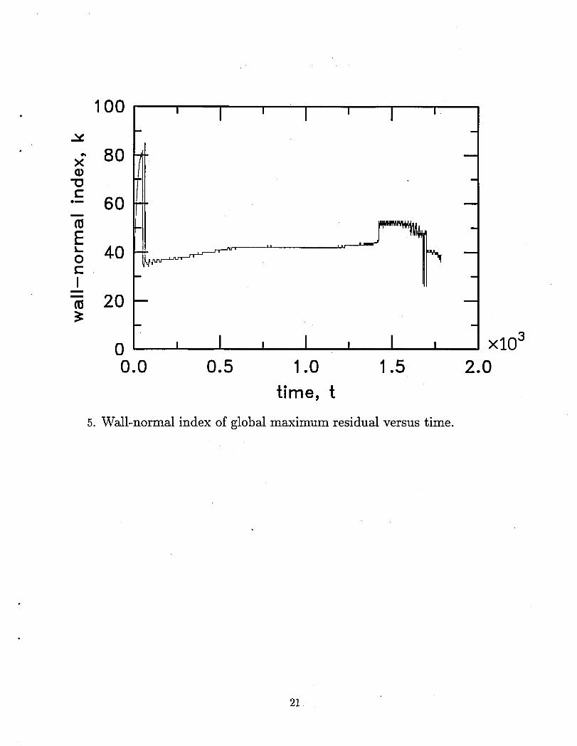
5. Wall-normal index of global maximum residual versus time.

21

6. Euler solution displaying isobars of constant pressure on upper andlower surfaces of wing model of Cattafesta et al. [3]

22

0.15 ; I ' I ' I ' I ;

0.10 -- I_

4--

' ' 0.05

0.00 -

-0.05 , I , I i I , I ,0.00 0.05 O.10 O.15 0.20 0.25

[ft]7. Wing section perpendicular to leading edge.

23

0.10 ' I ' I ' I ' I 'm

0.05

Upper Surface

o 0.00I

Lower Surface-0.05

-0.10 I v I , I v I ,0.0 0.2 0.4 0.6 0.8 1.0

Xc

8. Surface pressure coefficients for wing section of Fig. 7.

24

• 4.0 ' I ' I ' I ' I '

3.8 -/_ Euler _

:_°3"6 ............BE

3.4 ..............................................--....-- .3.2

3.0 , I , I , I , ,0.0 0.2 0.4 0.6 0.8 1.0

Xo

9. Edge Mach-number distribution for wing section of Fig. 7.

25.

210 _ I I I ' I i I ii

200 _- Euler -- :

,oo ii.iiiiiiii.i.i___*_-" 180 ................................... --i

170i

160

150 _ _ I w I i I _ I w0.0 0.2 0.4 0.6 0.8 1.0

Xc

10. Edge temperature distribution for wing section of Fig. 7.

26

• xlO -35 ' I ' I ' I ' I '

E

D

3--% -

2-m

1 -f u

0 , I , I , I , I ,0.00 0.05 0.10 0.15 0.20 0.25

S

X

11. Evolution of boundary'layer displacement thickness on upper surfaceof wing section of Fig. 7.

27

x10 3

2.5 I I ' I ' I ' I ' I 'i ..

,,z_,,.'_.";-'='_f °°

2.0- ,./ ," .

,. u(xo=O.OOO)/ o'

/ j/,'

=1. , (xo- oo) -5 - ,.. v -0 0/ st •

] j

>" " ( 3)-_.- ,.,,,, ......... u xc-O. 171.0 - ,Y , -

' (xc 73),......... v =01/,'

> /'0.5 , .--............................................................/ /

/ /"

/./" i

0.0 " ' I , I , I , I , I ,0 1 2 3 4 5 6

Z

12. Wall-normal distributions of streamwise and spanwise velocities at at-tachment line and at xc - 0.173 on upper wing surface.

28

• • . °

• 600 ' I ' I I I ' I I I '(9

• .'- 500 • (x_=O.OOO)r" _

•( _ )400 ',, ............T Xc-0.173 _

:_ ',

-,--'300 ,_1_ "IL ',

E 200 - "",................................................................................(1.)

100 , I , I , I , I , I0 1 2 3 4 5 6

Z

13. Wall-normal distribution of temperature at attachment line and at xc =0.173.

29#

xlO 32.5 I ' I ' I ' I ' I '

2.0

ffl_ 1.5 , --'+- ............"'c -i i

>- 10°_ _0-_ 0.5>

00. ......................................................................................

-0.50 1 2 • 3 4 5 6

Z

14. Comparison of tangential and crossflow velocities at xc = 0.173 onupper wing surface.

3O

100m

0 I ; I ; I ;0.0 0.2 0.4 0.6 0.8 1.0

Xc

15. Streamwise evolution of crossfiow Reynolds number on upper wing sur-face.

31

10° I ' I ' I ' I ' ---

10-1 i

-g lO-2 ............ _

E lO-3 DNS "-_ 10-4 ............PSE_.

, ......... suction on =10-5 i suction off --= i

E i =

10-6 - !,11 I , I , I , I ,0.0 0.2 0.4 0.6 0.8 1.0

X¢

16. Streamwise evolution of maximum of fundamental of spanwise velocityperturbation.

32

17. Contours of constant disturbance density in computational plane nor-mal to both leading edge and wing surface showing acoustic energygenerated by strong nonlinearity in wave-packet region.

33

1.2 ' I ' I ' I '- PSE-lines -

1.0 -- symbols _ ;

0.8

o. 0.6m0.4

0.2-- W --

oo__Z_¢_ ___'_ ___'° ° ×_°-_0 1 2 3 4

z

18.Comparison of amplitude distributions of componentsof fundamen-tal spanwiseFourier component of DNS ca]culation with PSE-derivedcrossflow disturbance at xc = 0.22. In each case,results are normal-ized so that maximum spanwise perturbation velocity is unity. (Evenindexed DNS values omitted.)

34

. 0.081 I ' I ' I ' I ' I '

• ,u _j \0.06 o

y* 0.04

0

0.02

0.000.00 0.02 0.04 0.06 0.08 0.10 0.12

X

19. Contours of constant perturbation density in surface approximately 1.5displacement thicknesses from wall showing alignment of crossflow vor-tices. Computational domain is replicated once in span for aesthetics.

35

0.010

0.005

0.000

-0.005

-0.010

-0.0150.00 0.02 0.04

*x

0.06 0.08 0.10

20. Projection of perturbation density field of Fig. 19 onto selected span­wise plane showing streamwise wavelength of dominant crossflow mode.

36

0.30.2

streamlinevortex (parallel)

vortex (nonparallel)DNS

........................... - -_ ", .. --'" -_ - -_ -_.--­_...----.--_ ...---_.-

o

0.1

,

\\\\\\.\\\\

\ ";'\ ".

" ." .

" ...." '.

".......

~ 80Ol

~ 78

76

740.0

90

88

00 86Q)

~ 84Ol

~ 82~

•

21. Comparison of vortex-alignment angle and inviscid-streamline anglerelative to x-axis showing orientation of crossflow mode in direction ofinviscid streamlines.

37

REPORT DOCUMENTATION PAGEForm ApprovedOMS No. 0704-0188

PlaJlic rwpofling burden lor lhill cohc:tian of inIormation ill _lIma.-d III average 1 hourper~.ilcUing ...1ime "" IWViewing inltNCliona, _rUling-.ng dllla -.......llIIltlering end ",,"nlallling ... data-.and completing and ......,;ng ... ccllecaon 01 inlormaliall. Send COIftlIWIII ::t:lQng lhiI.__or.., 0....Upeel oIlhi1 .cohc:tian oIlllormallorl.includI~1Ugge.1lorIs lor.-g h' burden... Wuhlngmn Heallquaners Selvice••~ r Intormalloll~1Ions end RePons. 1215~ 0...HJgIlwBy. Sun. 1204. Artllgton. A 22202~.lIIld III the 0IIIce 01 Management and Iludge~Papenoork Reduc1ion Project (0704-01881. ulinglDn. DC 20503.

1. AGENCY USE ONLY (t.-an tunk) /2. REPORT DATE /3. REPORT TYPE AND DATES COVERED

October 1995 Contractor Report4. mLE AND SUBmLE 5. FUNDING NUMBERS

Simulation of crossflow Instability on a Supersonic C NAS1-19656, Task 18Highly Swept Wing

WU 505-59-50-026. AUTHORIS)C. David Pruett

7. PERFORMING ORGANIZATION NAME(S) AND ADDRESSIES) 8. PERFORMING ORGANIZATIONThe College of William and Mary

REPORT NUMBER

Department of Applied Science

Hilliamsburg, VA 23185

II. SPONSORING I MONITORING AGENCY NAMEIS) AND ADDRESSIES) 10. SPONSORING I MONITORING

National Aeronautics and Space AdministrationAGENCY REPORT NUMBER

Langley Research CenterHampton, VA 23681-0001 NASA CR-198267

11. SUPPLEMENTARY NOTESLangley Technical Monitor: C. L. StreettFinal Report - Task 18

128. DISTRIBUTION I AVAILABIUTY STATEMENT 12b. DISTRIBUTION CODE

Unclassified - unlimited

Subject Category 02

13. ABSTRACT (MlIJCimum 200 wortU)

A direct numerical simulation (DNS) algorithm has been developed and validated foruse in the investigation of crossflow instability on supersonic swept wings, anapplication of potential relevance to the design of the High-speed Civil Transport(HSCT) . The algorithm is applied to the investigation of stationary crossflowinstability on an infinitely long 77-degree swept wing in Mach 3.5 flow. Theresults of the DNS are compared with the predictions of linear parabolizedstability equation (PSE) methodology. In general, the DNS and PSE results agreeclosely in terms of modal growth rate, structure, and orientation angle. Althoughfurther validation is needed for large-amplitude (nonlinear) disturbances, theclose agreement between independently derived methods offers preliminaryvalidation of both DNS and PSE approaches.

14. SUBJECT TERMS 15. NUMBER OF PAGES

Compressible Flow Crossflow Instability 38High-Speed Civil Transport IHSCT) Direct Numerical Simulation lOOS)

16. PRICE CODEParabolized Stability Equation IPSE) Methodology A03

17. SECURITY CLASSIFICATION 18. SECURITY CLASSIFICATION 111. SECURITY CLASSIFICATION 20. UMITATION OF ABSTRACTOF REPORT OF THIS PAGE OF ABSTRACT

Unclassified Unclassified Unclassified

NSN 754~1·2BO-5500 SlIIndard Form 2118 (Rev. 2-811)PNICribed by ANSI Sld. Z39-1 a298-102 .

· 1I1111111111111111f~~lIri[flljll~rlll~fliIlllllllllllll1113 1176014238258