jet in crossflow mixing
TRANSCRIPT

Effect of Jet Configuration on Transverse Jet Mixing Process
Sin Hyen Kim, Yonduck Sung, Venkat Raman
Department of Aerospace Engineering and Engineering MechanicsThe University of Texas at Austin
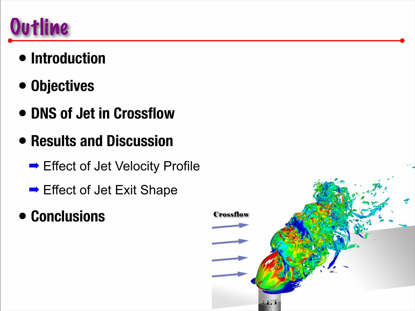
Outline• Introduction
• Objectives
• DNS of Jet in Crossflow
• Results and Discussion
➡ Effect of Jet Velocity Profile
➡ Effect of Jet Exit Shape
• Conclusions

Introduction : Transverse jet
• Transverse jet consist of crossflow and main jet
➡Can be found in many engineering applications
- Combustion chamber, chemical reactor
➡ How do we enhance mixing using transverse-jet?
Crossflowstream
Jet
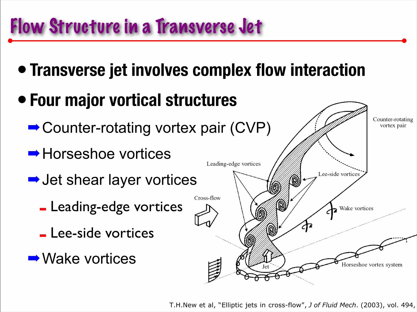
T.H.New et al, “Elliptic jets in cross-flow”, J of Fluid Mech. (2003), vol. 494, pp 119
Flow Structure in a Transverse Jet
• Transverse jet involves complex flow interaction
• Four major vortical structures
➡Counter-rotating vortex pair (CVP)
➡Horseshoe vortices
➡Jet shear layer vortices
- Leading-edge vortices
- Lee-side vortices
➡Wake vortices

Complexity of Vortical Structure
upstream vortices and the lee-side vortices, respectively.
These vortices resemble a ‘‘daisy chain’’ of interlocking
loops, which are similar to the buoyant jet structures ob-
served by Perry and Lim.41 What is interesting about these
loop vortices is that they were not produced by the bending
or folding of the vortex rings, as some researchers were led
to believe. In fact, there is no evidence of vortex rings in any
of our studies. This observation has also been made by Yuan
et al.27 in their large eddy simulation of a round jet in cross
flow.
To better understand how these loop vortices evolved,
video images of the flow field were replayed in slow motion.
They show that as soon as the cylindrical vortex sheet !seealso Fig. 1" emerged from the nozzle, it immediately folded
up on its edges to form a CVP. This finding is consistence
with the experimental observation of Kelso et al.,15 and the
large-eddy simulation of Yuan et al.27 Furthermore, it was
found that the CVP played a significant role in preventing
the cylindrical vortex sheet, which contains ‘‘circular’’ vor-
tex lines, from rolling up into vortex rings. This is in contrast
to the free jet, where the absence of CVP allows the vortex
sheet to roll up ‘‘axisymmetrically’’ into vortex rings. In the
case of JICF, the vortex sheet can roll up freely only at the
upstream and the lee-side of the jet column since the CVP
suppresses similar roll up at the two sides. This scenario
gives rise to two rows of loop vortices separated by the CVP
at the sides. Close examination shows that this formation
process is similar to the buoyant jet structures observed by
Perry and Lim,41 although the details are different. During
the folding of the vortex sheet, the fluid that originated from
the nozzle remained within the cylindrical boundary, and
there was no indication of holes or openings in the original
vortex sheet. This feature is clearly illustrated in Fig. 2,
where the jet fluid, which had been premixed with fluores-
FIG. 3. Authors’ interpretation of the
finally developed vortex structures of
JICF. !a" The sketch shows how the
‘‘arms’’ of both the upstream and the
lee-side vortex loops are merged with
the counter-rotating vortex pair. !b"Cross sectional views of !a" taken atvarious streamwise distances. Note
their close resemblance with the laser
cross sections of the jet depicted in
Fig. 5.
FIG. 4. Detailed sketches of the proposed model. !a" The sketch shows howthe vortex loops give rise to the resultant Section B-B. !b" Section E-E alongthe deflected jet centerline in the streamwise direction. This sketch repre-
sents the laser cross section of JICF depicted in Fig. 2.
772 Phys. Fluids, Vol. 13, No. 3, March 2001 Lim, New, and Luo
Downloaded 13 Nov 2008 to 146.6.102.83. Redistribution subject to AIP license or copyright; see http://pof.aip.org/pof/copyright.jsp
Lim et al, “On the development of large-scale structures of a jet normal to a cross flow”, Phys of Fuild (2001), Vol. 13, pp 770
Crossflowstream
Jet
Initiation of CVP

Jet Mixing Control Parameter
• Velocity ratio results in higher trajectory and more efficient mixing
• Thicker crossflow boundary layer results in higher trajectory, but less efficient mixing
• What is the effect of jet configuration?
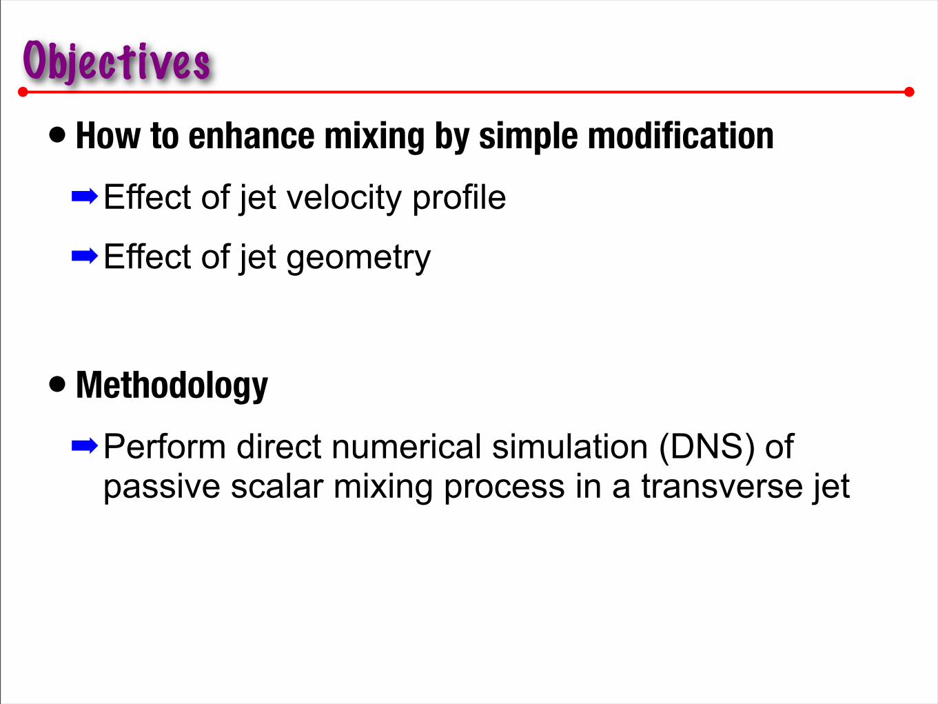
Objectives• How to enhance mixing by simple modification
➡Effect of jet velocity profile
➡Effect of jet geometry
• Methodology
➡Perform direct numerical simulation (DNS) of passive scalar mixing process in a transverse jet

DNS of Jet in Crossflow
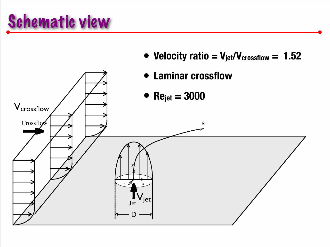
Schematic view
• Velocity ratio = Vjet/Vcrossflow = 1.52
• Laminar crossflow
• Rejet = 3000
z x
y
u∞
Crossflow
Jet
s
D
Vjet
Vcrossflow

Governing Equations
Figure 1: A sketch of a crossflow jet system.
The motivation for this work is the optimization of a crossflow chemical reactor. The reactants,contained in the two jets, react with infinitely fast chemistry. However, the product can further reactwith one of the reactants to produce secondary unwanted products. Optimization of this systemwill require minimization of the secondary reactions caused mainly by the recirculation producedat the lower-wall. Consequently, the main jet velocity compared to the crossflow jet should be highenough to ensure that the product trajectory is high above the lower boundary flow, and shouldcarry sufficient momentum to ensure rapid mixing. However, this increased velocity will alsoincrease the power requirements and pressure losses thereby increasing the operating costs. Theobjective of this study is to determine if modifiying the jet exit shape can enhance mixing rates atlower velocity ratios while still limiting the secondary reactions. Two different jet exit shapes, asquare and circular shape, are compared to determine mixing patterns.
B. Direct numerical simulation of crossflow jets
Fig. 1 shows a schematic of the problem. The incompressible flow equations are solved using anenergy conserving numerical scheme. The continuity and momentum equations are given by
∂uj
∂xj= 0
∂ui
∂t+
∂uiuj
∂xj=
1
ρ
�−∂P
∂xi+
∂τij
∂xj
�, (1)
where ui is the velocity component, ρ is the constant fluid density, P is the local pressure, and τij
is the viscous stress tensor.τij = −2
3µ
∂uk
∂xkδij + 2µSij, (2)
Sij =1
2
�∂ui
∂xj+
∂uj
∂xi
�, (3)
Figure 1: A sketch of a crossflow jet system.
The motivation for this work is the optimization of a crossflow chemical reactor. The reactants,contained in the two jets, react with infinitely fast chemistry. However, the product can further reactwith one of the reactants to produce secondary unwanted products. Optimization of this systemwill require minimization of the secondary reactions caused mainly by the recirculation producedat the lower-wall. Consequently, the main jet velocity compared to the crossflow jet should be highenough to ensure that the product trajectory is high above the lower boundary flow, and shouldcarry sufficient momentum to ensure rapid mixing. However, this increased velocity will alsoincrease the power requirements and pressure losses thereby increasing the operating costs. Theobjective of this study is to determine if modifiying the jet exit shape can enhance mixing rates atlower velocity ratios while still limiting the secondary reactions. Two different jet exit shapes, asquare and circular shape, are compared to determine mixing patterns.
B. Direct numerical simulation of crossflow jets
Fig. 1 shows a schematic of the problem. The incompressible flow equations are solved using anenergy conserving numerical scheme. The continuity and momentum equations are given by
∂uj
∂xj= 0
∂ui
∂t+
∂uiuj
∂xj=
1
ρ
�−∂P
∂xi+
∂τij
∂xj
�, (1)
where ui is the velocity component, ρ is the constant fluid density, P is the local pressure, and τij
is the viscous stress tensor.τij = −2
3µ
∂uk
∂xkδij + 2µSij, (2)
Sij =1
2
�∂ui
∂xj+
∂uj
∂xi
�, (3)where µ is the constant fluid viscosity. To study mixing in these jets, a passive scalar was also
evolved along with the flow equations.
∂φ
∂t+
∂ujφ
∂xj=
∂
∂xj
�D
∂φ
∂xj
�, (4)
where φ is the scalar mass-fraction and D is the scalar diffusivity, which was assumed to be the
same as the fluid viscosity.
The above equations were solved using a finite-volume projection-based solver. The convection
terms in the momentum equations were discretized using a second-order energy conserving central
scheme. The convection term in the scalar transport equation was discretized using a third-order
upwind-biased scheme. This upwind bias was necessary to reduce unphysical oscillations in the
scalar transport equation. The viscous and diffusion terms were discretized using a second-order
central scheme. The time advancement is based on a semi-implicit predictor-corrector algorithm.
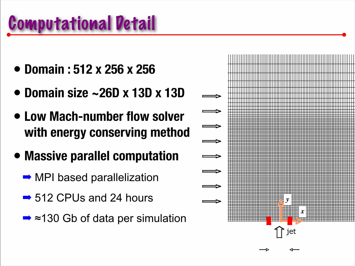
The computational domain spans 26D× 13D× 13D, where D is the diameter of the main jet. The
jet Reynolds number was fixed at 5000 while the main flow Reynolds number was set to 1500,
yielding a velocity ratio of 1.52. This particular ratio was chosen so that direct comparison with
prior experiments could be carried out for validation purposes. To resolve the smallest length-
scales in the flow, over 30 million computational points (512 × 256 × 256) were required. To
capture the near-field dynamics, the grid was clustered in all directions close to the jet entrance.
The focus of this study is the effect of jet exit shape on mixing. For this purpose, both the incoming
crossflow and the main jet were assumed to be laminar. The crossflow boundary layer thickness
just before the main jet entrance was approximately equal to the jet diameter for all the studies
considered. For the square jet, the inlet area was set such that the mass flow rate is equal to that of
the circular exit case.
All computations were carried out on massively parallel computers. A domain decomposition
strategy using an MPI-based distributed computing paradigm was used. Separate studies demon-
strated that the code scales efficiently up to 512 processors. The simulations performed here used
between 128 and 512 processors and were carried out on the Lonestar computing system operated
by the Texas Advanced Computing Center (TACC). Each simulation took roughly 20 hours from
start to completion for over the five residence times.
C. Results and Discussion
The discussion below is based on steady state profiles obtained from the two simulations involving
a circular jet and a square jet. The simulations were carried out long enough to ensure that statistics
were stationary. Here, the flow behavior is analyzed using the vorticity and passive-scalar evolution
fields.
Fluid vorticity provides an excellent measure of the large-scale fluid circulation in turbulent flows.
Here, the vorticity is computed from the steady-state three-dimensional velocity fields. Essentially,
this Reynolds-averaged computation of vorticity will indicate the regions of large-scale recircula-
tion that are responsible for jet breakup and mixing. This vorticity field is shown in Fig. 2 for both
jet exit shapes. All crossflow jets exhibit a horseshoe vortex pattern, seen in Fig. 2, on the floor
from which the main jet is issuing. This feature represents the strong curvature of the crossflow
Incompressible Navier Stokes Equation
Passive scalar transport equation
jet
yx
Computational Detail
• Domain : 512 x 256 x 256
• Domain size ~26D x 13D x 13D
• Low Mach-number flow solver with energy conserving method
• Massive parallel computation
➡ MPI based parallelization
➡ 512 CPUs and 24 hours
➡ ≈130 Gb of data per simulation

jet
yx
Grid convergence test
• Tested three grid set to validate the result from 512x256x256
➡ 256x128x128
➡ 512x256x256
➡ 1024x512x512

Mean passive scalar field256
512 1024
1 rsd = 0.5 sec
~0.65 rsd2 rsd
2 rsd
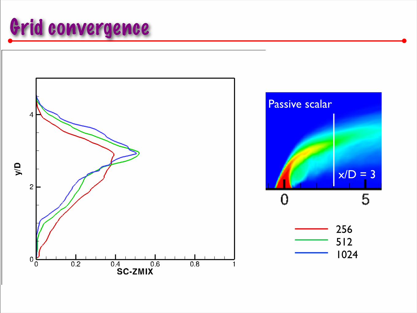
Grid convergence
2565121024
x/D = 3
Passive scalar
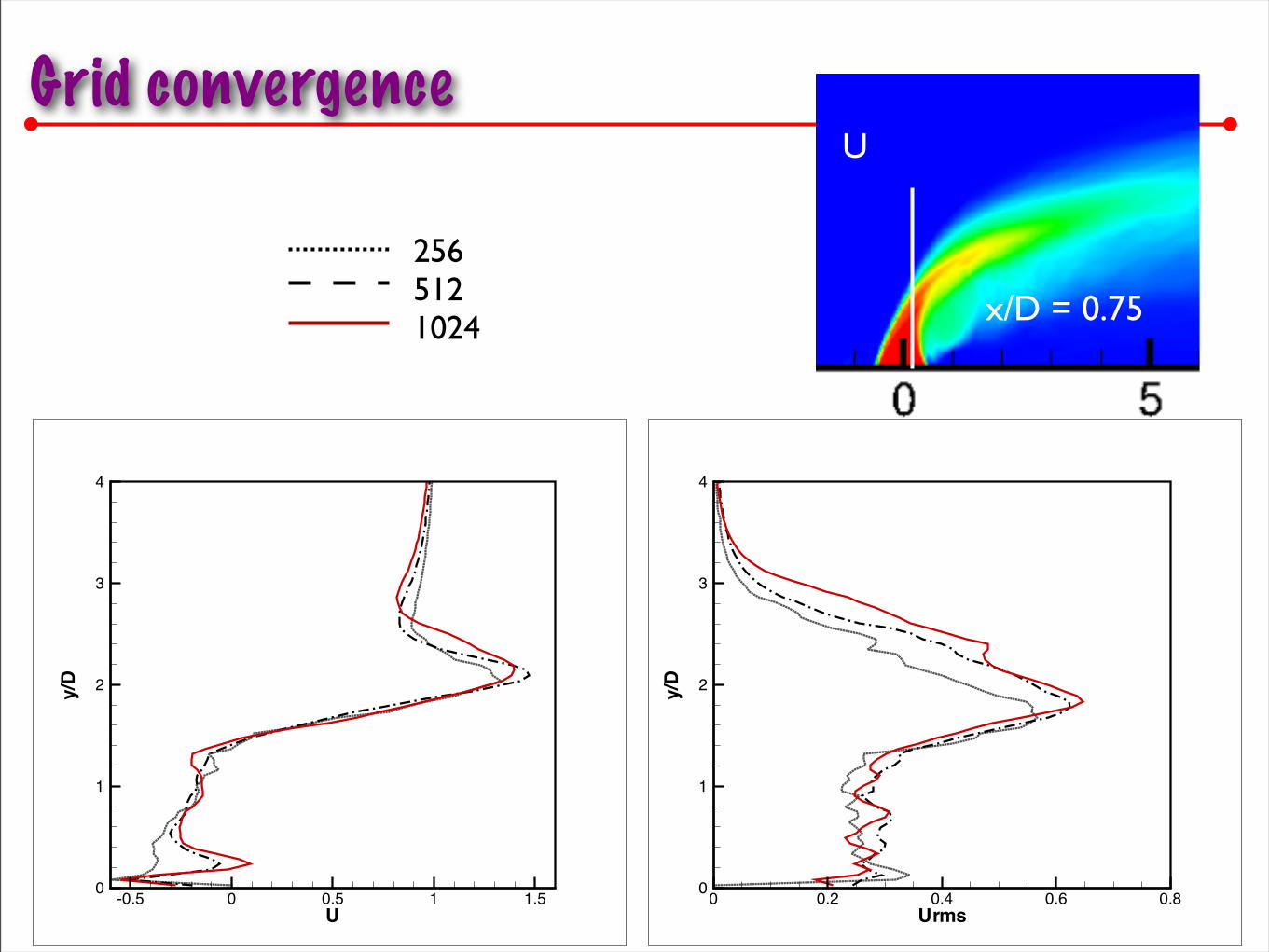
Grid convergence
2565121024 x/D = 0.75
U
Urms
y/D
0 0.2 0.4 0.6 0.80
1
2
3
4
U
y/D
-0.5 0 0.5 1 1.50
1
2
3
4
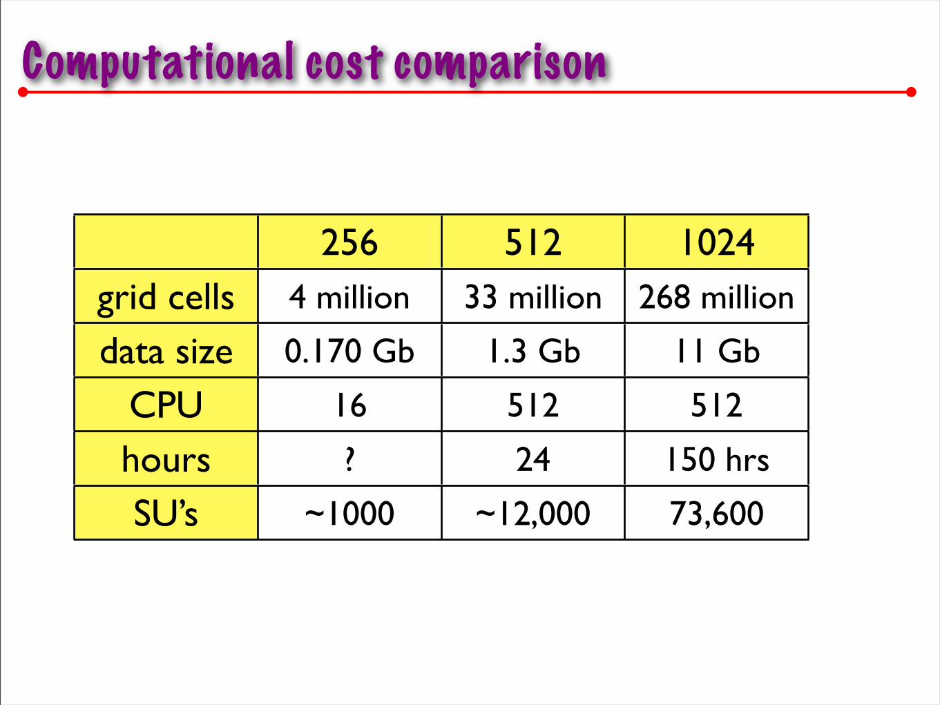
Computational cost comparison
256 512 1024grid cells 4 million 33 million 268 million
data size 0.170 Gb 1.3 Gb 11 Gb
CPU 16 512 512
hours ? 24 150 hrs
SU’s ~1000 ~12,000 73,600
Results and Discussion
1. Effect of Jet Velocity Profile
2. Effect of Jet Shape
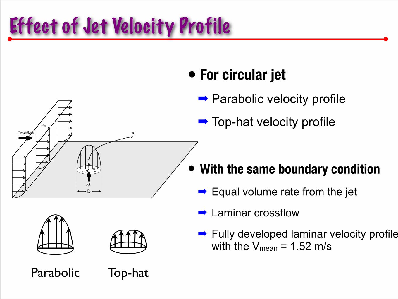
Effect of Jet Velocity Profile
z x
y
u∞
Crossflow
Jet
s
D
• For circular jet
➡ Parabolic velocity profile
➡ Top-hat velocity profile
• With the same boundary condition
➡ Equal volume rate from the jet
➡ Laminar crossflow
➡ Fully developed laminar velocity profile with the Vmean = 1.52 m/s
Parabolic Top-hat
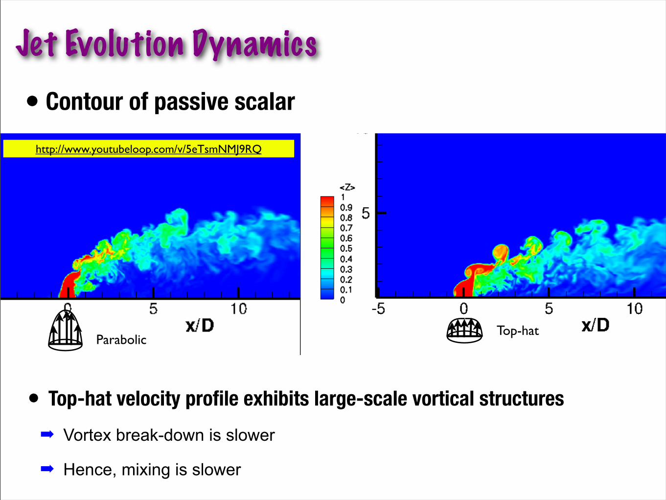
Top-hat
Jet Evolution Dynamics
Parabolic
• Top-hat velocity profile exhibits large-scale vortical structures
➡ Vortex break-down is slower
➡ Hence, mixing is slower
• Contour of passive scalar
http://www.youtubeloop.com/v/5eTsmNMJ9RQ
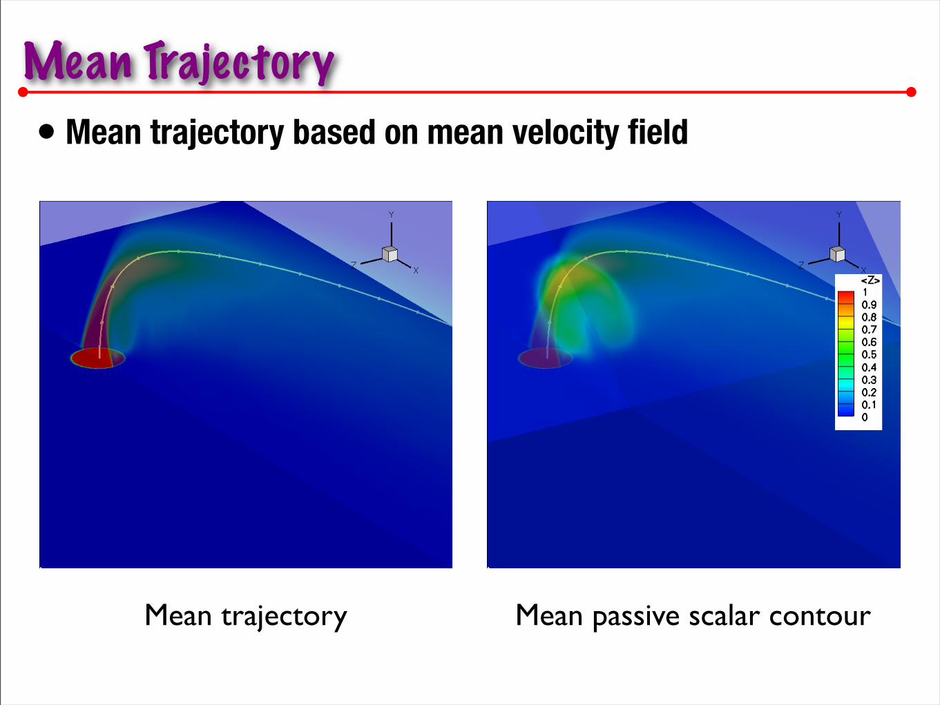
Mean Trajectory• Mean trajectory based on mean velocity field
Mean trajectory Mean passive scalar contour
x/D
y/D
5 10 150
1
2
3
4
5
6
Parabolic
Top-hat
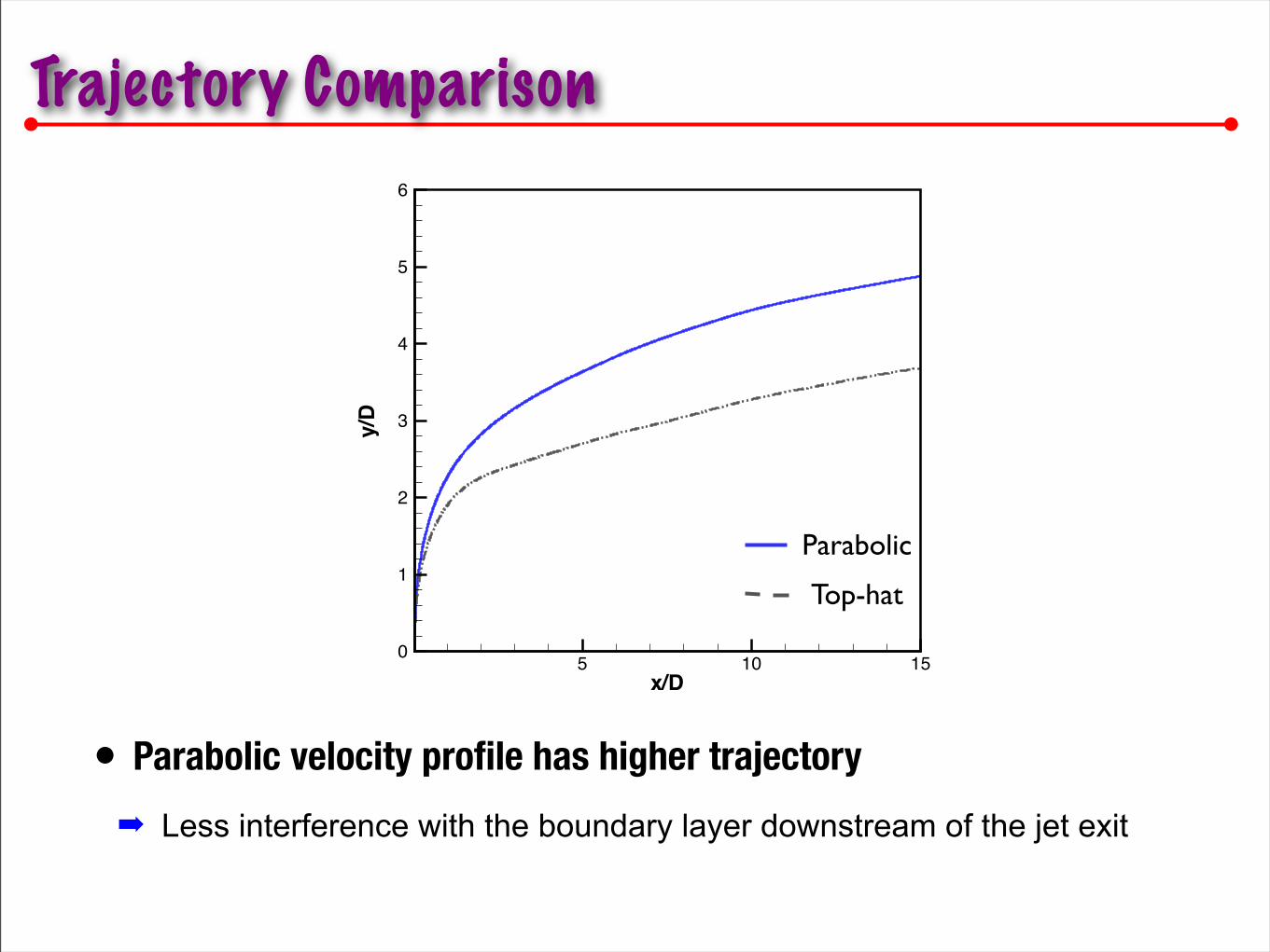
Trajectory Comparison
• Parabolic velocity profile has higher trajectory
➡ Less interference with the boundary layer downstream of the jet exit

x/D
5 10 15 200
0.05
0.1
0.15
Mixing along centerline trajectory
x/D5 10 15 20
0.2
0.4
0.6
0.8
1
Parabolic
Top-hat
• Passive scalar along the mean trajectory
Mean passive scalar along the trajectory Variance of mean passive scalar along the trajectory
Parabolic
Top-hat
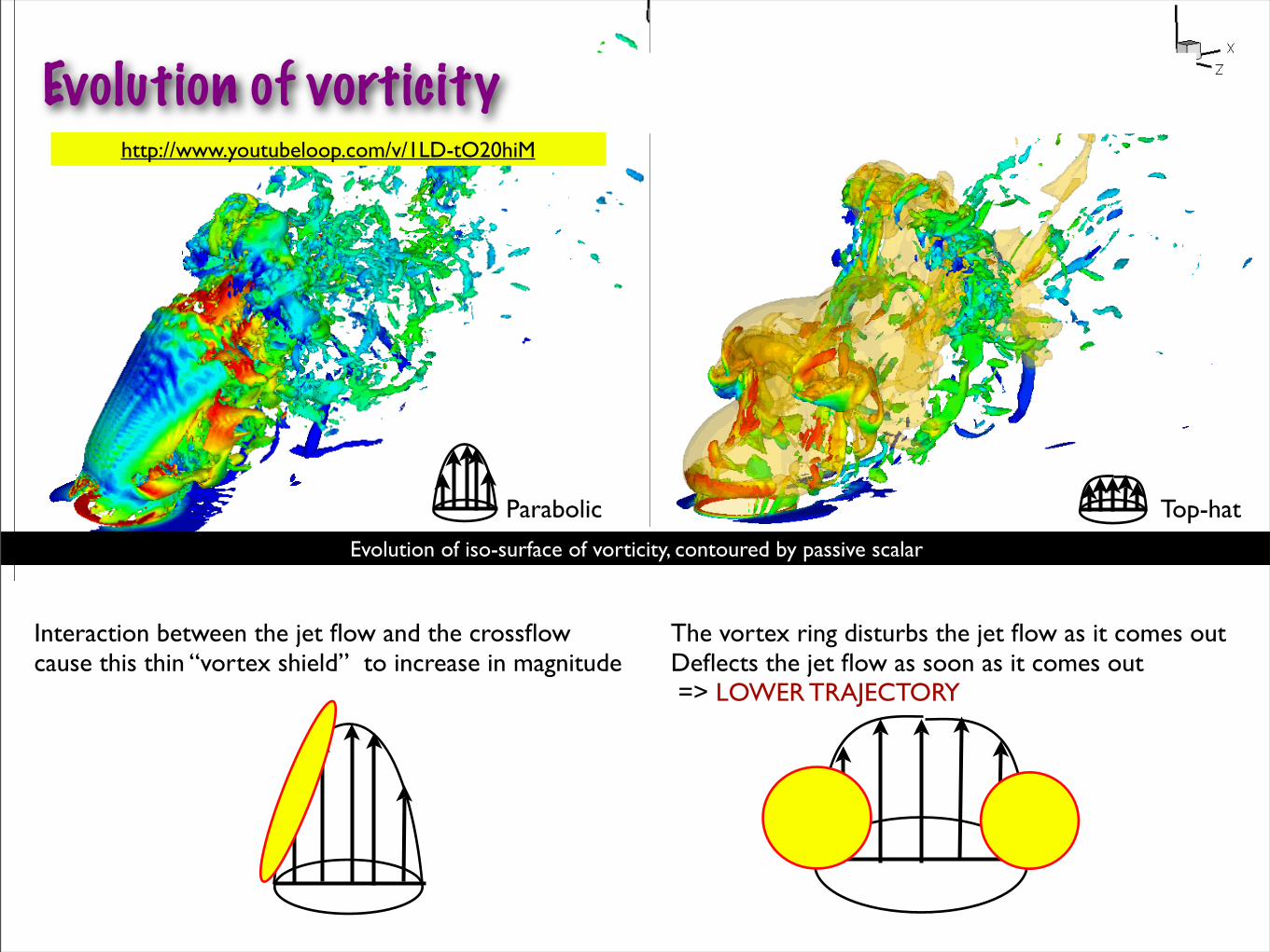
Evolution of iso-surface of vorticity, contoured by passive scalar
Parabolic Top-hat
Evolution of vorticity
The vortex ring disturbs the jet flow as it comes outDeflects the jet flow as soon as it comes out => LOWER TRAJECTORY
Interaction between the jet flow and the crossflowcause this thin “vortex shield” to increase in magnitude
http://www.youtubeloop.com/v/1LD-tO20hiM
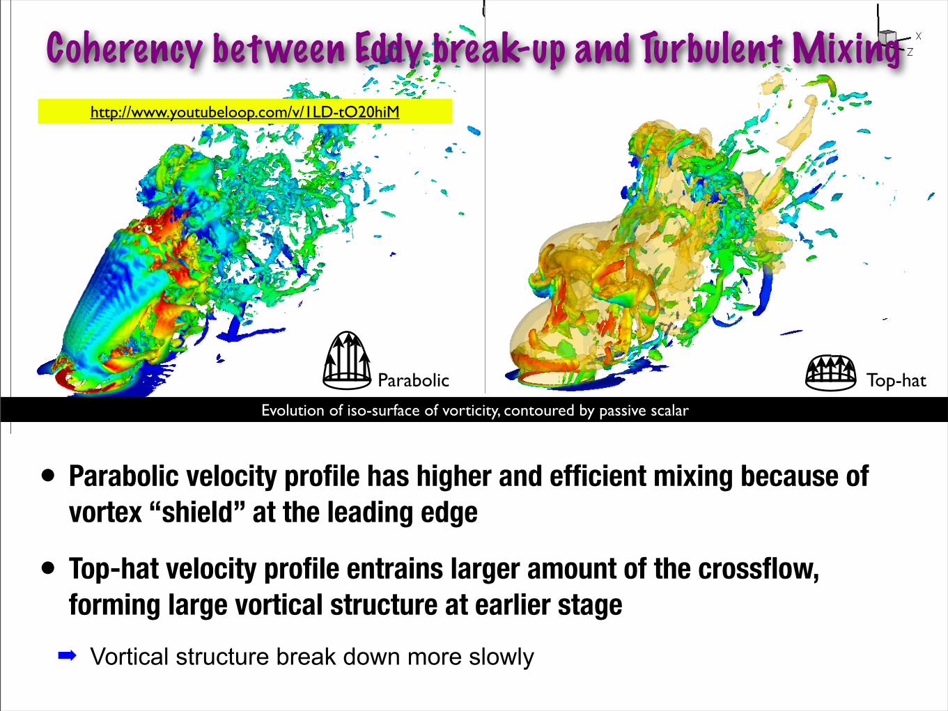
Coherency between Eddy break-up and Turbulent Mixing
Parabolic Top-hat
Evolution of iso-surface of vorticity, contoured by passive scalar
• Parabolic velocity profile has higher and efficient mixing because of vortex “shield” at the leading edge
• Top-hat velocity profile entrains larger amount of the crossflow, forming large vortical structure at earlier stage
➡ Vortical structure break down more slowly
http://www.youtubeloop.com/v/1LD-tO20hiM

z x
y
u∞
Crossflow
Jet
s
D
Effect of Jet Exit Shape• Four different geometries were chosen for comparison
• With the same boundary condition
➡ Equal volume rate from the jet
➡ Laminar crossflow
➡ Fully developed laminar velocity profile with the Vmean = 1.52 m/s
Circle SquareTriangle
1Triangle
2D

Jet Evolution Dynamics
CircleTriangle
1
• Contour of passive scalar
http://www.youtubeloop.com/v/5eTsmNMJ9RQ http://www.youtubeloop.com/v/mrfaa8bzk4s
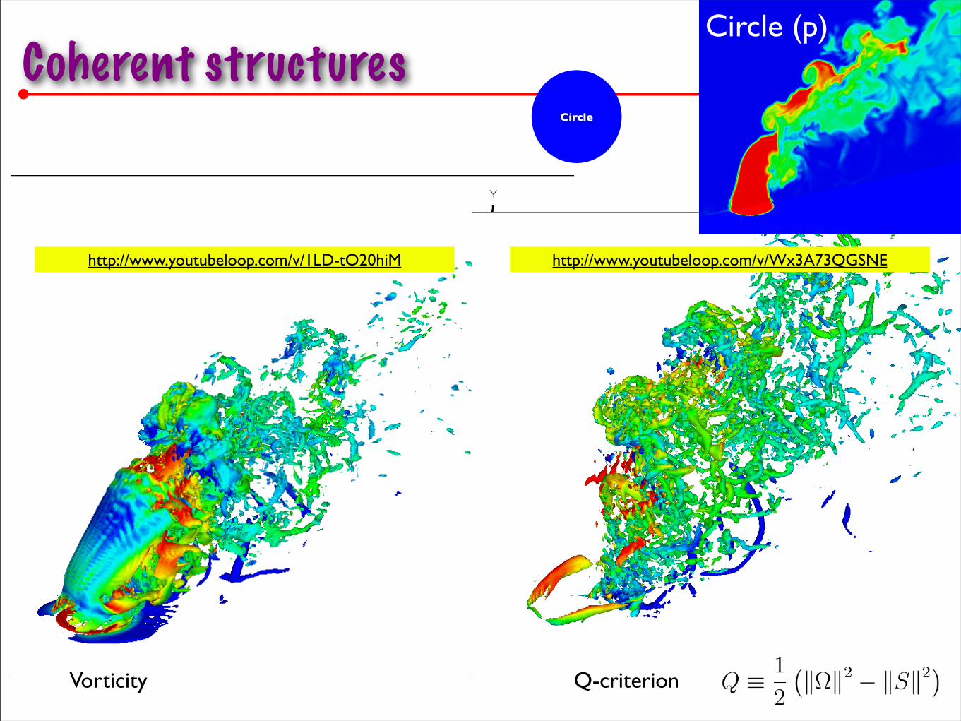
Coherent structuresCircle (p)
Circle
Vorticity Q-criterion
http://www.youtubeloop.com/v/1LD-tO20hiM http://www.youtubeloop.com/v/Wx3A73QGSNE

T.H.New et al, “Elliptic jets in cross-flow”, J of Fluid Mech. (2003), vol. 494, pp 119
Flow Structure in a Transverse Jet
• Four major vortical structures
➡Counter-rotating vortex pair (CVP)
➡Horseshoe vortices
➡Jet shear layer vortices
- Leading-edge vortices
- Lee-side vortices
➡Wake vortices
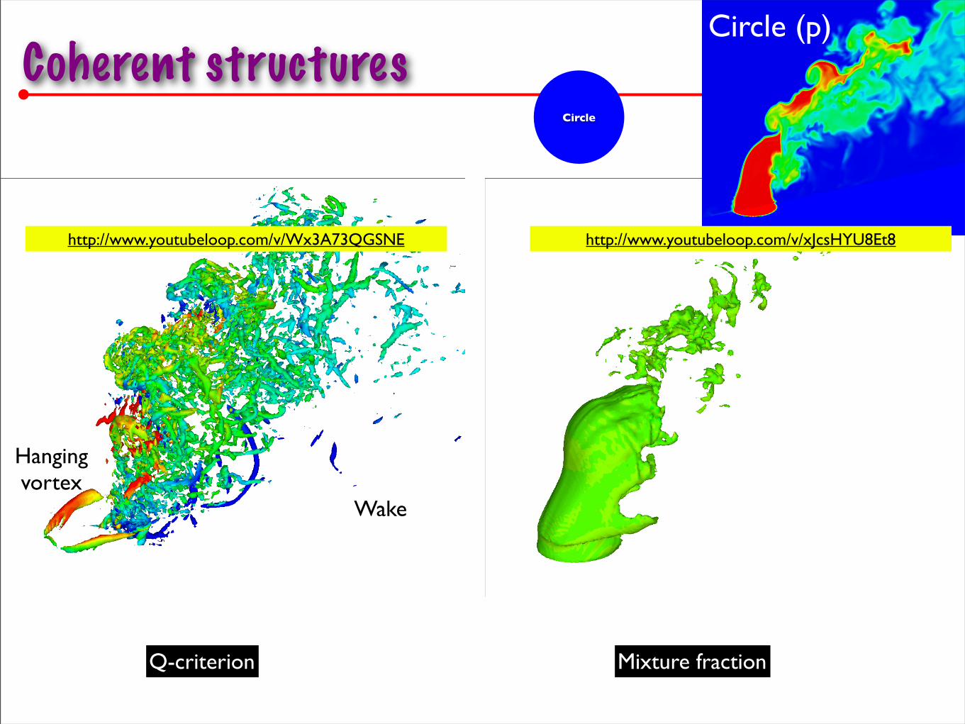
Coherent structuresCircle (p)
Circle
Q-criterion Mixture fraction
Wake
Hanging vortex
http://www.youtubeloop.com/v/Wx3A73QGSNE http://www.youtubeloop.com/v/xJcsHYU8Et8
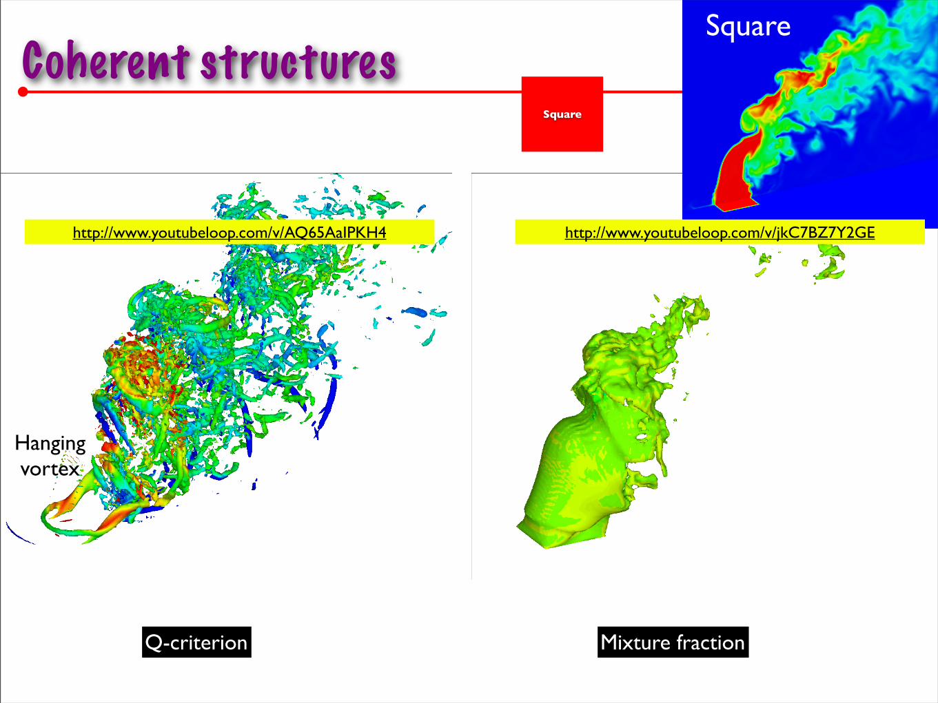
Coherent structuresSquare
Square
Hanging vortex
Q-criterion Mixture fraction
http://www.youtubeloop.com/v/AQ65AaIPKH4 http://www.youtubeloop.com/v/jkC7BZ7Y2GE
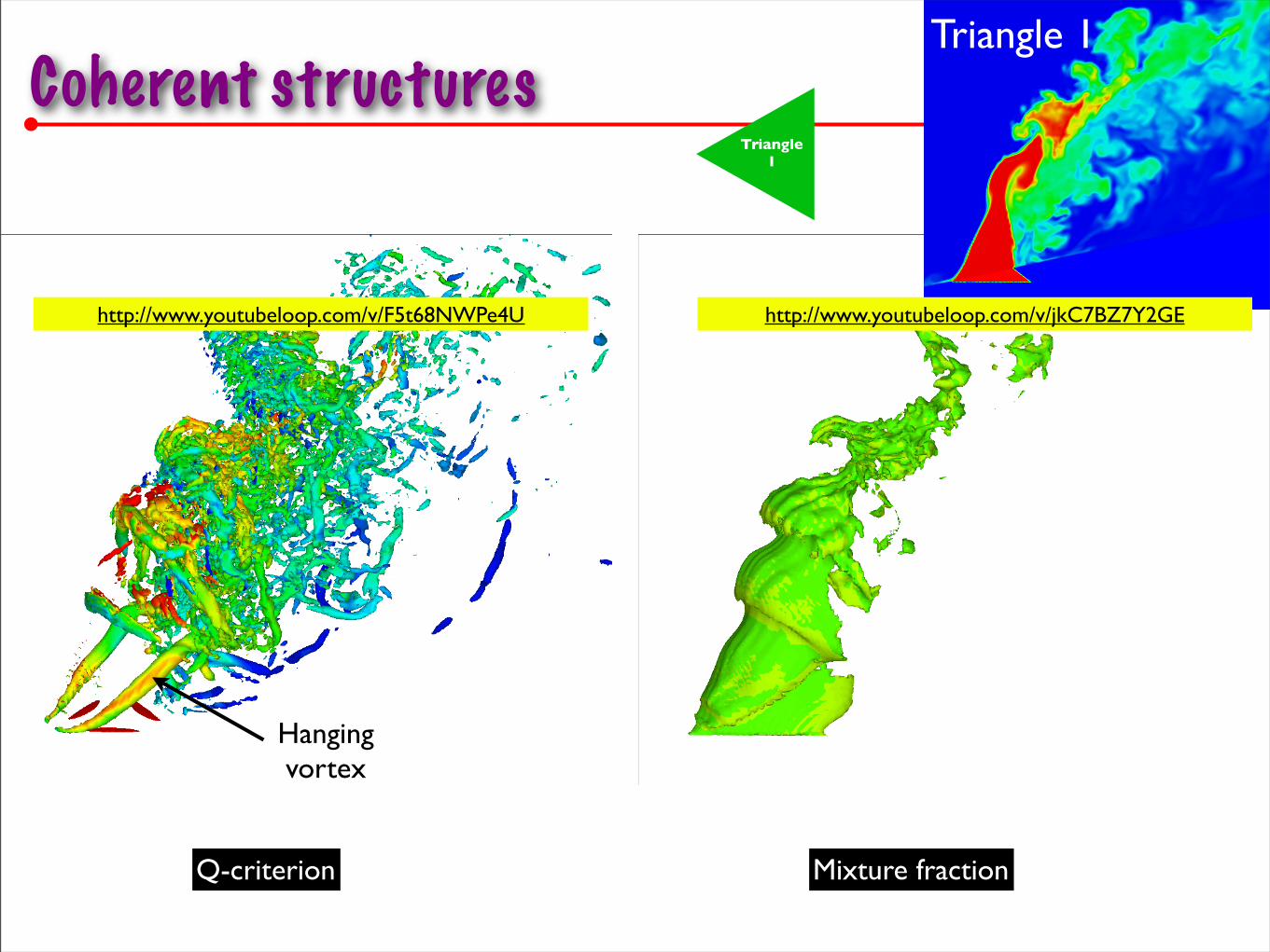
Coherent structuresTriangle 1
Triangle 1
Hanging vortex
Q-criterion Mixture fraction
http://www.youtubeloop.com/v/F5t68NWPe4U http://www.youtubeloop.com/v/jkC7BZ7Y2GE

Coherent structuresTriangle 2
Triangle 2
Hanging vortexHorseshoe
vortices
Q-criterion Mixture fraction
http://www.youtubeloop.com/v/1Q6sh9TBcjk http://www.youtubeloop.com/v/_-QIzG3zxGw
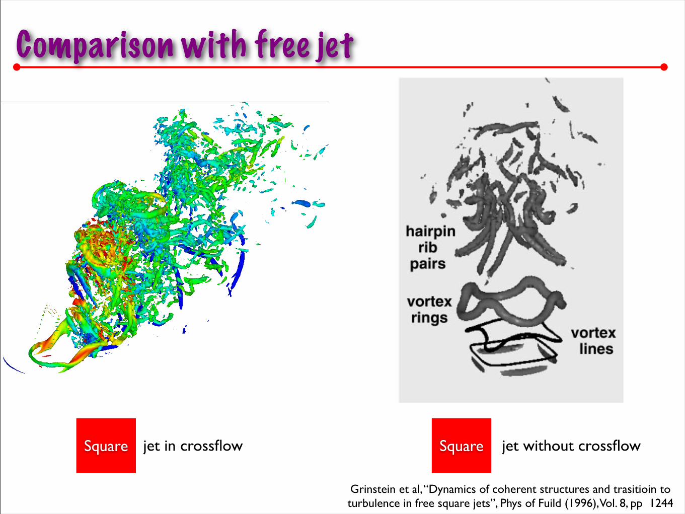
Comparison with free jetSquare
Square
P1: NBL/mbg/spd P2: NBL/ary QC: ARS
November 16, 1998 17:1 Annual Reviews AR075-07
FLOW CONTROL WITH NONCIRCULAR JETS 265
Figure 14 Interacting ring and braid vortices for low-AR rectangular free jets with AR= 1.Instantaneous visualizations at two consecutive times based on vorticity isosurfaces and vortex
lines. (Grinstein & DeVore 1996)
Strong interactions with braid vortices and other rings can inhibit axis rotations
of nonisolated rings, which do not recover shape and flatness after the initial
self-deformation.
In the square jet case (Grinstein & DeVore 1996), for example, braid (hair-
pin) vortices induce flow ejection at the corner regions and flattening of the
ring portions left behind after the initial ring self-deformation (Figure 14), and
this mechanism leads to the second axis rotation of the jet cross-section. This
is in contrast with the self-induced axis-rotation dynamics of isolated rings, a
process in which ring shape and flatness are approximately recovered. In terms
of jet spreading along characteristic directions, axis rotations first require faster
growth on the flat sides (s-direction) and shrinking along the vertex direction
(d-direction) so that crossover of jet widths along ‘s’ and ‘d’ is possible. The
self-distortion of the corner regions of the vortex ring is the mechanism under-
lying the initial shrinking along ‘d,’ depending directly on the local azimuthal
curvature C and thickness σ (according to Equation 1). The dependence of
An
nu
. R
ev.
Flu
id M
ech
. 1
99
9.3
1:2
39
-27
2.
Do
wn
load
ed f
rom
arj
ou
rnal
s.an
nu
alre
vie
ws.
org
by
Un
iver
sity
of
Tex
as -
Au
stin
on
09
/30
/09
. F
or
per
son
al u
se o
nly
.
jet in crossflow Square jet without crossflow
Grinstein et al, “Dynamics of coherent structures and trasitioin to turbulence in free square jets”, Phys of Fuild (1996), Vol. 8, pp 1244
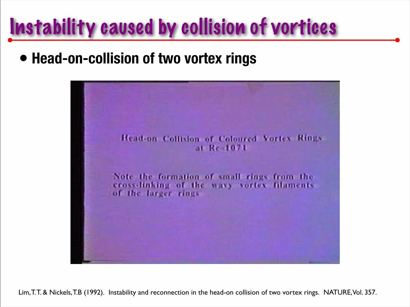
Instability caused by collision of vortices• Head-on-collision of two vortex rings
Lim, T. T. & Nickels, T.B (1992). Instability and reconnection in the head-on collision of two vortex rings. NATURE, Vol. 357.
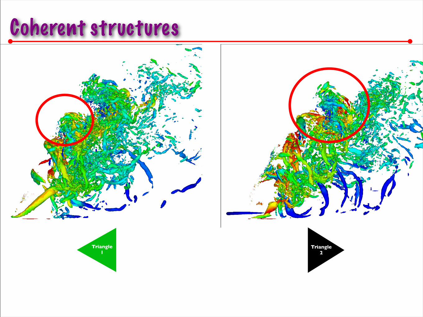
Coherent structuresTriangle 1
Triangle 1
Triangle 2
x/D
y/D
0 5 10 150
1
2
3
4
5
6
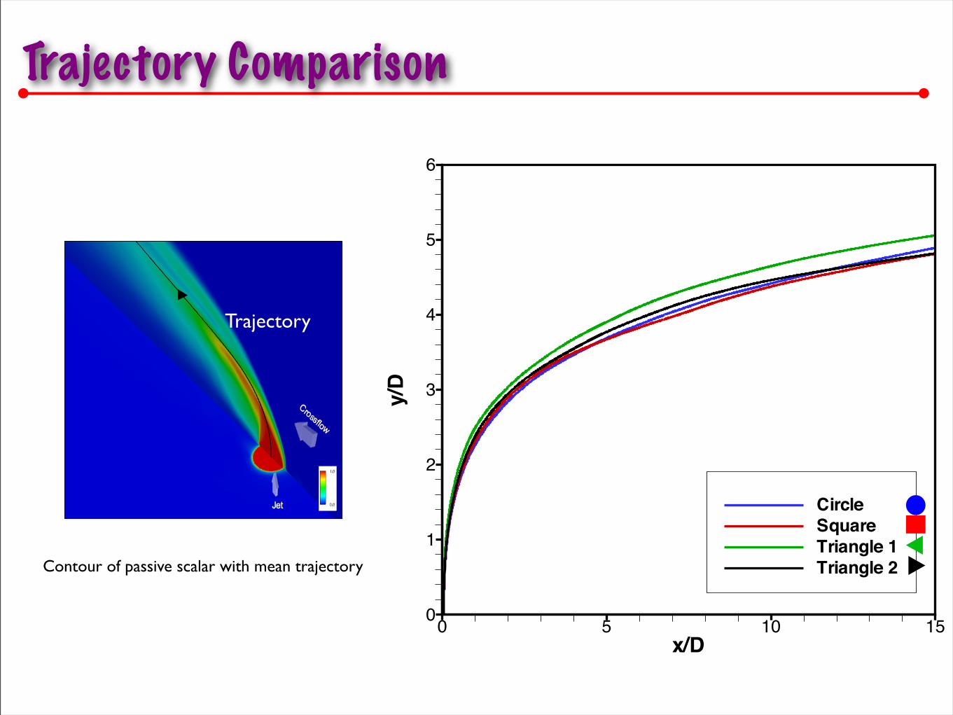
CircleSquareTriangle 1Triangle 2
Trajectory Comparison
Contour of passive scalar with mean trajectory
Trajectory

• Passive scalar along the mean trajectory
x/D
SC-ZMIX
0 5 10 150.00
0.20
0.40
0.60
0.80
1.00
CircleSquareTriangle 1Triangle 2
x/D
Var
0 5 10 150.00
0.02
0.04
0.06
0.08
0.10
CircleSquareTriangle 1Triangle 2
Mean passive scalar along the trajectory Variance of mean passive scalar along the trajectory
Near-field Far-field
Mixing along centerline trajectory

Near-Field Flow Evolution
CircleTriangle
1
• Mean passive scalar contour
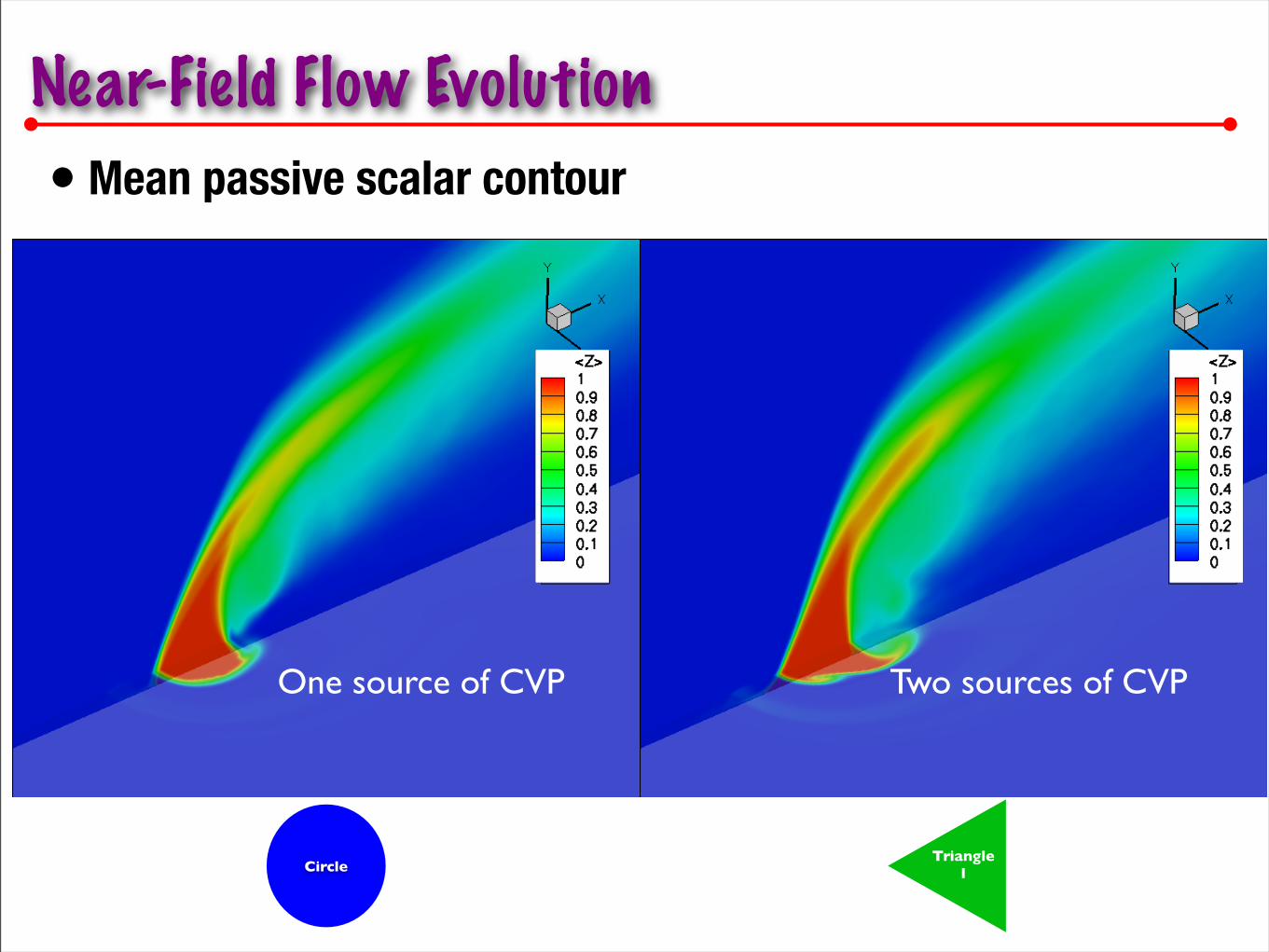
One source of CVP Two sources of CVP
CircleTriangle
1
Near-Field Flow Evolution• Mean passive scalar contour
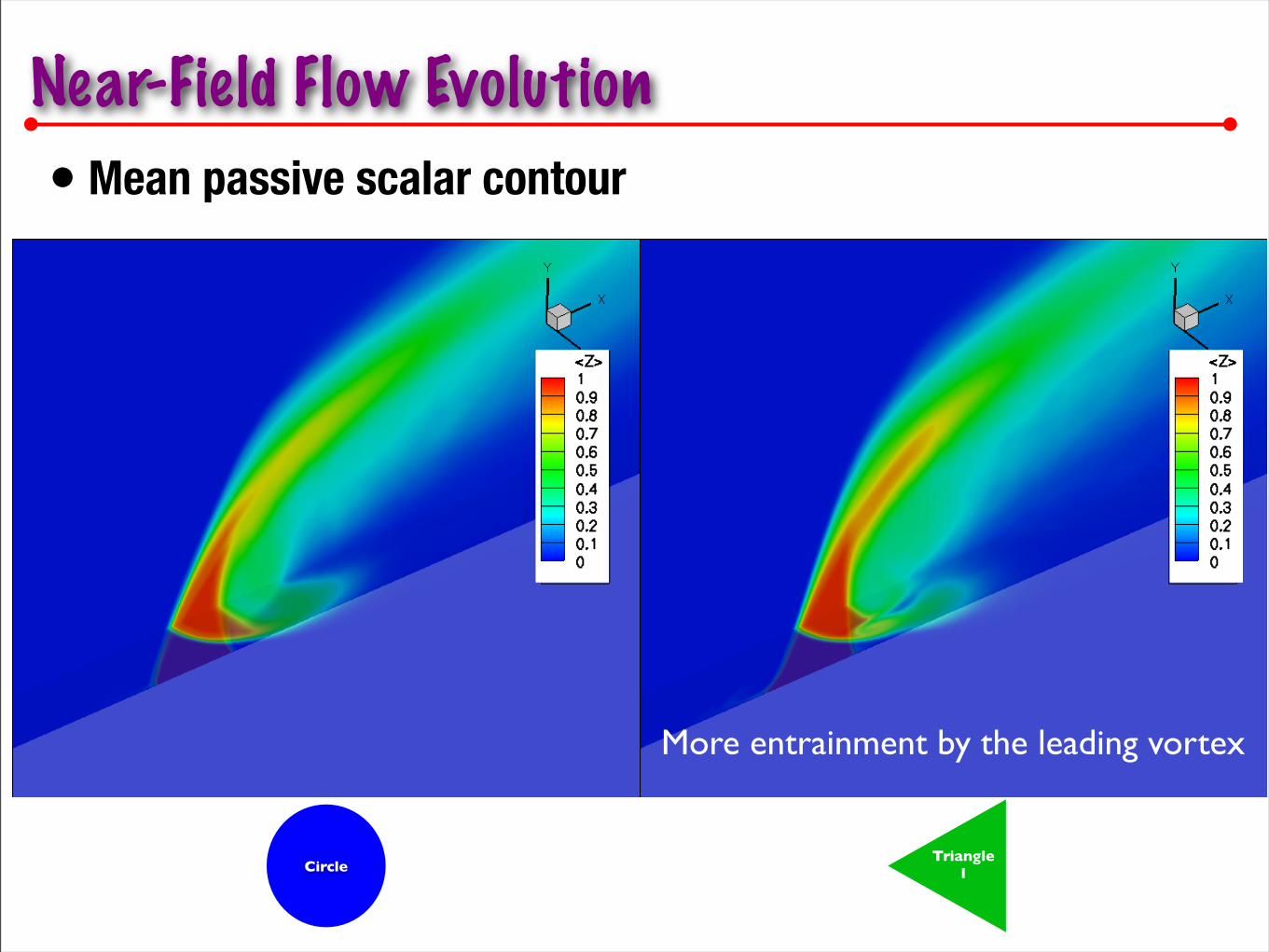
More entrainment by the leading vortex
CircleTriangle
1
Near-Field Flow Evolution• Mean passive scalar contour

CircleTriangle
1
Two vortices merged together
Near-Field Flow Evolution• Mean passive scalar contour
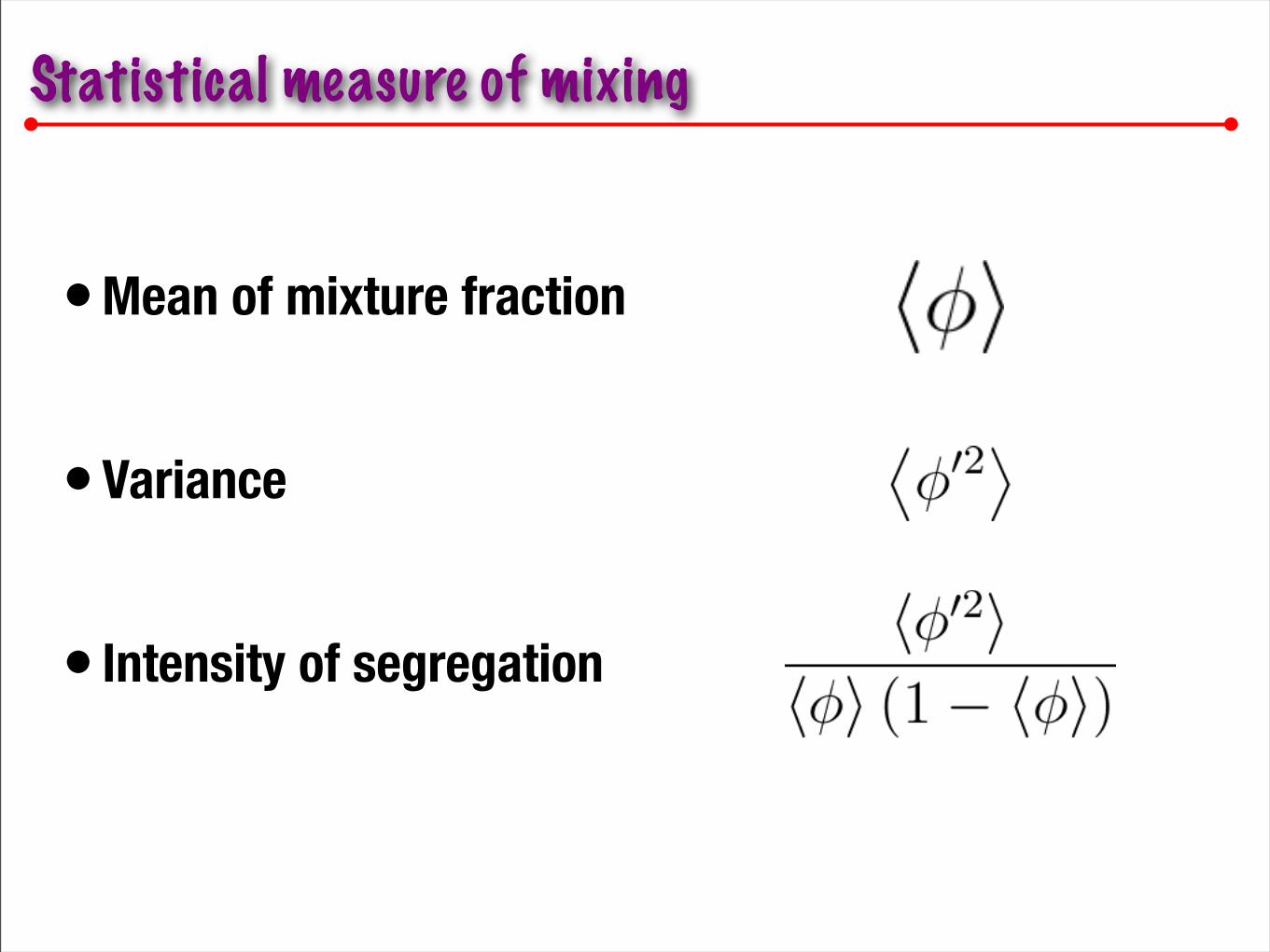
Statistical measure of mixing
•Mean of mixture fraction
•Variance
• Intensity of segregation

Circular (parabolic)
Variance
Intensity of segregation
Circle
Mean of mixture fraction

Circular (tophat)
Variance
Intensity of segregation
Circle
Mean of mixture fraction

Square
Variance
Intensity of segregation
Square
Mean of mixture fraction

Mean of mixture fraction
Upstream Triangle
Variance
Intensity of segregation
Triangle 1
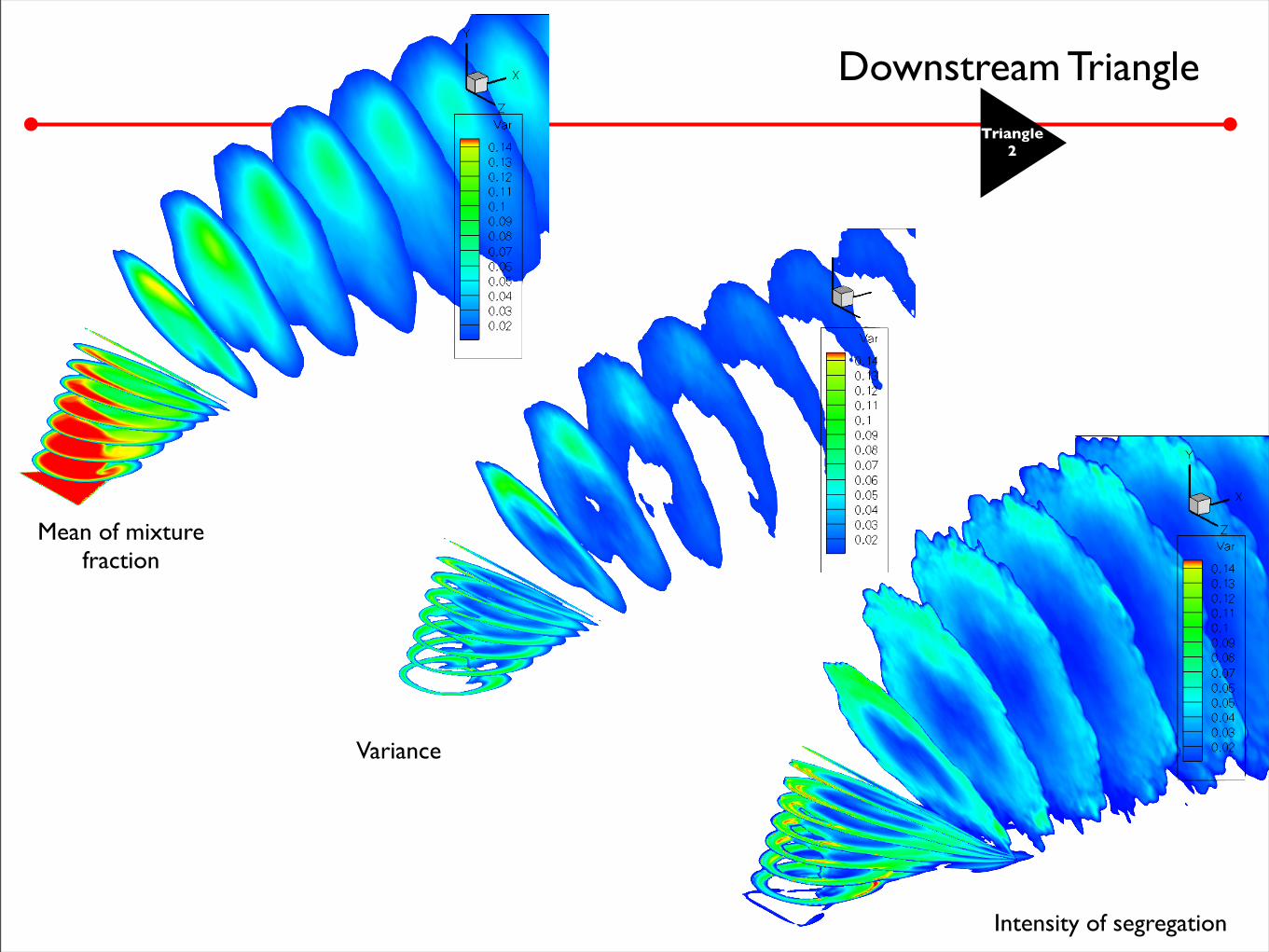
Downstream Triangle
Variance
Intensity of segregation
Triangle 2
Mean of mixture fraction
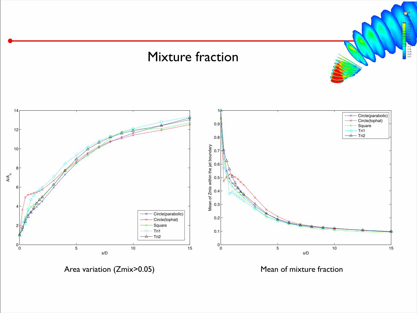
Mixture fraction
0 5 10 150
2
4
6
8
10
12
14
s/D
A/A o
Circle(parabolic)Circle(tophat)SquareTri1Tri2
0 5 10 150
0.1
0.2
0.3
0.4
0.5
0.6
0.7
0.8
0.9
1
s/D
Mea
n of
Zm
ix w
ithin
the
jet b
ound
ary
Circle(parabolic)Circle(tophat)SquareTri1Tri2
Area variation (Zmix>0.05) Mean of mixture fraction
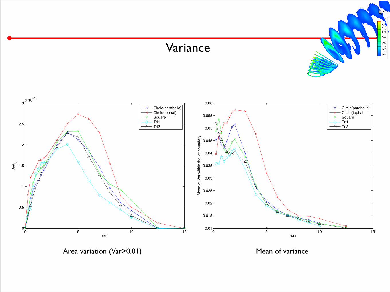
Variance
0 5 10 150
0.5
1
1.5
2
2.5
3x 10 3
s/D
A/A o
Circle(parabolic)Circle(tophat)SquareTri1Tri2
0 5 10 150.01
0.015
0.02
0.025
0.03
0.035
0.04
0.045
0.05
0.055
0.06
s/D
Mea
n of
Var
with
in th
e je
t bou
ndar
y
Circle(parabolic)Circle(tophat)SquareTri1Tri2
Area variation (Var>0.01) Mean of variance
0 5 10 150
5
10
15
20
25
30
35
40
s/D
A/A o
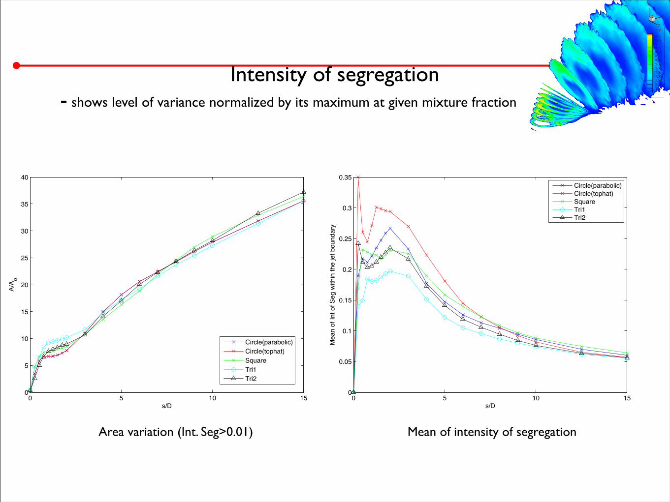
Circle(parabolic)Circle(tophat)SquareTri1Tri2
0 5 10 150
0.05
0.1
0.15
0.2
0.25
0.3
0.35
s/D
Mea
n of
Int o
f Seg
with
in th
e je
t bou
ndar
y
Circle(parabolic)Circle(tophat)SquareTri1Tri2
Intensity of segregation- shows level of variance normalized by its maximum at given mixture fraction
Area variation (Int. Seg>0.01) Mean of intensity of segregation
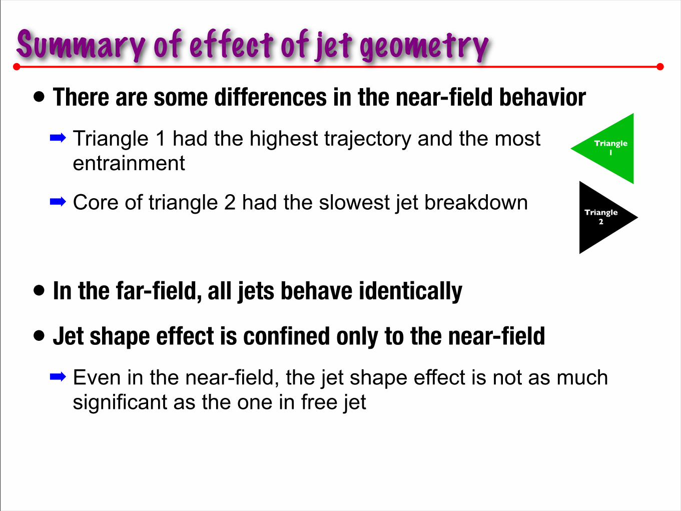
Summary of effect of jet geometry• There are some differences in the near-field behavior
➡ Triangle 1 had the highest trajectory and the most entrainment
➡ Core of triangle 2 had the slowest jet breakdown
• In the far-field, all jets behave identically
• Jet shape effect is confined only to the near-field
➡ Even in the near-field, the jet shape effect is not as much significant as the one in free jet
Triangle 1
Triangle 2

Conclusion• Effect of transverse-jet geometry was studied
➡Jet exit geometry cause minor impact on overall mixing process
➡For circular jet, velocity profile affects both trajectory and mixing condition
- Parabolic jet has higher trajectory and develops more favorable condition for turbulent mixing by interacting with the crossflow
- Top-hat jet entrains the crossflow earlier in near-field, but mixing is slower