cortés mora-valencia perote (2017) implicit probability ... filethe implicit rnd in the option...
TRANSCRIPT

No. 17-23 2017
Implicit probability distribution for WTI options: The Black Scholes vs. the semi-nonparametric approach
Lina M. Cortés, Andrés Mora-Valencia, and Javier Perote

Implicit probability distribution for WTI options:
The Black Scholes vs. the semi-nonparametric approach
Lina M. Cortés*+, Andrés Mora-Valencia **, and Javier Perote***
* Universidad EAFIT, Medellín, Colombia
** Universidad de los Andes, School of Management, Bogotá, Colombia
*** University of Salamanca (IME), Salamanca, Spain
Abstract
This paper contributes to the literature on the estimation of the Risk Neutral Density (RND)
function by modeling the prices of options for West Texas Intermediate (WTI) crude oil that
were traded in the period between January 2016 and January 2017. For these series we extract
the implicit RND in the option prices by applying the traditional Black & Scholes (1973)
model and the semi-nonparametric (SNP) model proposed by Backus, Foresi, Li, & Wu
(1997). The results obtained show that when the average market price is compared to the
average theoretical price, the lognormal specification tends to systematically undervalue the
estimation. On the contrary, the SNP option pricing model, which explicitly adjust for
negative skewness and excess kurtosis, results in markedly improved accuracy.
Keywords: Oil prices, option pricing, risk neutral density, semi-nonparametric approach
JEL Classification: Q47, G12, C14
+ Corresponding author: Department of Finance, School of Economics and Finance, Universidad EAFIT, Carrera 49 No 7 Sur-50, Medellin, Colombia. E-mail: [email protected]. Fax: +57 43120649. Other authors’s e-mails: [email protected] (Javier Perote), [email protected] (A. Mora-Valencia).
1. Introduction
The fluctuation of oil prices over recent years has caused huge concern among consumers,
firms and governments (Huang, Yu, Fabozzi, & Fukushima, 2009; Kallis & Sager, 2017).
On a global level, forecasting macroeconomic variables is largely impacted by oil price
projections, given that economic activity and inflation are dependent on them (He, Kwok, &
Wan, 2010; Kallis & Sager, 2017). The difficulty is due to the fact that oil prices are strongly
influenced by stock levels, the weather, the short-term imbalances between supply and
demand, and political issues (Huang, Yu, Fabozzi, & Fukushima, 2009; de Souza e Silva,
Legey, & de Souza e Silva, 2010; Abhyankar, Xu, & Wang, 2013). However, as the Risk
Neutral Density (RND) function reflects the market expectations on the future development
of the underlying assets, such density has become a useful tool to model the price of this
commodity (Jondeau & Rockinger, 2000; Liu, Shackleton, Taylor, & Xu, 2007; Monteiro,
Tütüncü, & Vicente, 2008; Fabozzi, Tunaru, & Albota, 2009; Du, Wang, & Du, 2012; Lai,
2014; Taboga, 2016; Kiesel & Rahe, 2017).
The prices of financial options are a valuable source of information to be able to obtain the
RND (Liu, 2007; Rompolis, 2010; Völkert, 2015). Hence, this research seeks to contribute
to the literature on estimating the RND through modeling WTI crude oil options that are
priced on the New York Mercantile Exchange (NYMEX) commodity market. Different
methods have been developed to extract the RND; however, their efficiency must be tested
in several types of markets and not only in the stock market (on which the majority of studies
have been focused) (see, for example, Corrado & Su, 1996; Corrado & Su, 1997; Hartvig,
Jensen, & Pedersen, 2001; Lim, Martin, & Martin, 2005; Monteiro, Tütüncü, & Vicente,
2008; Birru & Figlewski, 2012; Christoffersen, Heston, & Jacobs, 2013; Kiesel & Rahe,
2017; Leippold & Schärer, 2017; etc.). The very fact that oil continues to be a fundamental
energy component in modern economies is an important reason to study the behavior of
option prices for the WTI. Changes in oil prices can produce important effects on the global
economy, which means it is important to create new methods that allow for the stochastic
process of the future price to be adjusted (Abhyankar, Xu, & Wang, 2013; Su, Li, Chang, &
Lobonţ, 2017).

The theory based on which modeling the prices of financial assets was developed began with
the publication of the Black-Scholes (1973) valuation model. This seminal work has been the
basis for many generalizations and enhancements by academics and finance professionals
(Peña, Rubio, & Serna, 1999; Liu, 2007; León, Mencía, & Sentana, 2009; Rompolis, 2010;
Du, Wang, & Du, 2012; Lai, 2014; Feng & Dang, 2016). However, the Black-Scholes model
has become less reliable over time. Even for markets for which it was expected to be more
precise, there have been differences between the theoretical prices and the market prices
(Jarrow & Rudd, 1982; Corrado & Su, 1996; Backus, Foresi, Li, & Wu, 1997; Birru &
Figlewski, 2012; Christoffersen, Heston, & Jacobs, 2013).
It is known that after the stock market crisis of October 1987, the Black-Scholes option
valuation model tended to underestimate the options that are very much ‘in-the-money’ and
‘out-of-the-money’ (see Rubinstein (1994) for a detailed discussion of this empirical
regularity). This is the result of the violation of the assumption under which all option prices
for the same underlying asset with the same expiration date but with a different exercise price
should have the implied volatility (Corrado & Su, 1997; Lim, Martin, & Martin, 2005;
Friesen, Zhang, & Zorn, 2012). The empirical evidence reveals that the implied volatility
derived from the Black-Scholes model seems to be different across the exercise price by
drawing the well-known volatility smile (Peña, Rubio, & Serna, 1999; Jondeau & Rockinger,
2000; Liu, 2007; Kiesel & Rahe, 2017).
The Black-Scholes model assumes that the RND is lognormal, but this prediction has been
convincingly rejected by (MacBeth & Merville, 1979). Hence, the literature on option pricing
has suggested models that allow for adjustments to be included, both in terms of bias and
excess kurtosis in the RND, in order to correct the previously mentioned problems (Backus,
Foresi, Li, & Wu, 1997; Nikkinen, 2003; Jondeau, Poon, & Rockinger, 2007, p. 365; Friesen,
Zhang, & Zorn, 2012). The relevance of these types of models lies in the assumption that the
logarithm of the share price being normal is unrealistic, specifically because the distribution’s
tails are heavier than those that have a normal distribution (Fama, 1965; Das & Sundaram,
1999; Dennis & Mayhew, 2002; Nikkinen, 2003; Huang, Yu, Fabozzi, & Fukushima, 2009;
Feng & Dang, 2016).
To this effect, the most up-to-date academic literature has taken two different directions to
try to measure the RND. The first consists of specifying a stochastic process of the alternative
price different to that proposed by Black-Scholes, which, in turn, results in an alternative
RND. The second seeks to develop procedures to extract implicit RND from the option prices
observed (Hartvig, Jensen, & Pedersen, 2001; Dennis & Mayhew, 2002; Lai, 2014). In line
with the second direction, Breeden & Litzerberger (1978), Shimko (1993) and Jondeau,
Poon, & Rockinger (2007, p. 398) suggest making use of the fact that the RND is the second
derivative from the call option price with respect to the exercise price.
However, other authors have proposed different approaches such as: parametric ones, which
suggest a direct expression for the RND without referring to the specific price dynamics
(Ritchey, 1990; Melick & Thomas, 1997; Anagnou-Basioudis, Bedendo, Hodges, &
Tompkins, 2005; Fabozzi, Tunaru, & Albota, 2009; Völkert, 2015); nonparametric ones that
do not try to give an explicit form of the RND (Jackwerth & Rubinstein, 1996; Aït-Sahalia
& Lo, 1998); and semi-nonparametric ones (SNP) that suggest an approximation of the RND
(Jarrow & Rudd, 1982; Corrado & Su, 1996; Backus, Foresi, Li, & Wu, 1997; Rompolis &
Tzavalis , 2007; León, Mencía, & Sentana, 2009; Taboga, 2016).
This study’s approach seeks to extract the RND that is implicit in the option prices by
applying an SNP model. Specifically, we verify whether the SNP model proposed by Backus,
Foresi, Li, & Wu (1997) outperforms option pricing measures for the WTI listed in the period
between January 2016 and January 2017. Additionally, for the purpose of contrasting the
results obtained, the dates that are being analyzed are either special events in the oil market
and political events that have the ability to affect the financial markets or days of “relative”
calm. In the first stage, the skewness parameters and excess kurtosis are calibrated by using
the SNP distribution. In the second stage, the previously estimated parameters (skewness and
excess kurtosis) are used to approximate the price distribution of the underlying asset under
a specification that we write as log-SNP.1 The advantage of applying SNP models is that they
are not as data intensive as other methods, which allows for the RND to be extracted (Aït-
1 The Black-Scholes approach considers that the price of an underlying asset is distributed under a lognormal specification in the sense that its variations follow a normal distribution. As is demonstrated in Section 2, the Gram-Charlier or SNP distribution corresponds to an extention of the normal distribution, and the log-SNP corresponds to an extention of the log-normal distribution. Consequently, the SNP option valuation model is a generalization of the Black-Scholes model.

Sahalia & Lo, 1998; Taboga, 2016). Given that there is scanty number of price data obtained
from the financial markets in a trading day, it is essential the seach of a method which fit the
data in an accurate way for practioners so as they can take optimal decisions (Liu, 2007; Feng
& Dang, 2016).
Backus, Foresi, Li & Wu (1997) use a Gram-Charlier A series expansion (hereafter denoted
as SNP) around a normal density function to incorporate the terms of adjustment for
skewness and excess kurtosis for the Black-Scholes formula. These authors used the model
suggested by Jarrow & Rudd (1982) as a baseline; they were pioneers in proposing an SNP
model for valuing options using an Edgeworth series expansion around the lognormal density
function. Subsequently, Corrado & Su (1996) also derived a valuation model for option prices
using a Gram-Charlier series expansion around the normal density function.
Although Corrado & Su’s (1996) model is derived from Jarrow & Rudd (1982), operationally
the pioneers explain the bias deviations and the excess kurtosis of the lognormality of the
share price while the model developed by Corrado & Su (1996) explain the deviations from
normality of the asset returns in terms of bias and excess kurtosis. It is noteworthy that Brown
& Robinson (2002) have corrected two of Corrado & Su’s (1996) typographical errors and
they provide examples of how errors such as these may have economic significance. We
adopt the Backus, Foresi, Li, & Wu (1997) model in this study because these authors show
that some of the terms in Corrado & Su’s (1996) model are numerically very small in real
markets and can be eliminated from the option pricing model. As such, Backus, Foresi, Li,
& Wu (1997) propose a more parsimonious model that represents a good approximation of
the option price.
This paper is divided into the following sections: Section 2 presents the model to be estimated
and the applied methodology. Section 3 describes the data that will be used. Section 4 gathers
the results and discusses the suggested method, and, finally, Section 5 summarizes the
conclusions.

2. Model and methodology
2.1. Model
The first attempt to estimate the RND was developed by Breeden & Litzerberger (1978). The
authors demonstrated that the RND can be recovered from the second derivative of the call
price. ! (") is a European call (put) option with exercise price # and the time at expiration%,
! #; ' = )*+,-.
/0 − # 2 /0; ' 3/0, (1)
" #; ' = )*+,.5
# − /0 2 /0; ' 3/0, (2)
where 6 is the risk-free rate. Hence,
789
7.8 .:;<= )*+,2 /0; ' . (3)
The term )*+,2 /0 is generally referred to as the state price density (SPD), and 2 . is the
undiscounted RND (Jondeau, Poon, & Rockinger, 2007, p. 387). The estimation of the RND
by (3) requires a continuous series of exercise prices to estimate the parameters by using a
finite differences method. However, this procedure leads to unstable results and, in turn,
several methods such as (i) local volatility or implied tree models, (ii) interpolation of the
implied volatility curve, (iii) stochastic volatility and jumps, (iv) nonparametric approach,
and (v) the combination of parametric and nonparametric approaches that have been
suggested in the literature (see, for example, Fusai & Roncoroni, 2008 and the references
therein). This research uses a classic parametric approach from the lognormal approximation
and its achievements can be compared with the SNP suggested approach, which is explained
in the following subsection.
2.2. Methodology
For a particular date and for various call and put option contracts with the same expiration
and different exercise prices, the Black-Scholes and SNP models’ set of parameters' is
estimated by minimizing the sum of the squared errors between the observed market prices
and the theoretical prices, and the parameter set is used to represent the RND for each model.

In the first step, the parameters (>,?,@A,@B) are callibrated by using the Black-Scholes and
SNP models for call and put options. These parameters are used in the second step to fit the
probability density function (pdf) by assuming a lognormal distribution and log-SNP,
respectively.2
The well-known theoretical price for the Black-Scholes call option is given by,
!C; #; ' = /0D 3E − #)*+,D 3F , (4)
where D . denotes the cumulative distribution function (cdf) of the normal standard, 3E =
GH /0 # + 6 + ?F 2 % ? %. Moreover, the call option price of the SNP model can be
formulated as (Backus, Foresi, Li, & Wu, 1997; Christoffersen, 2012, p. 237):
!;KL #; ' = !C; #; ' + /0M 3E ? @A 2 %? − 3E − @B % 1 − 3EF + 33E %? − 3%?F . (5)
The put prices are obtained through the Put–call parity. In order to obtain (5), the log-returns
are assumed to be Gram-Charlier distributed instead of Gaussian as in the case of Black-
Scholes. The pdf of the Gram-Charlier distribution is given by:
P Q = 1 + @RSR QTR:E M Q , (6)
where @R are the parameters and the Gram-Charlier distribution3 and SR Q is the sth order
Hermite polynomial (HP), which can be defined in terms of the derivatives of normal
standard density M Q , such as UVW X
UXV= −1 RSR Q M Q .
Specifically, the four first HP are:
SE Q = Q, (7)
SF Q = QF − 1, (8)
2The methodology used in this paper was developed based on the R Package Risk Neutral Density Extraction Package (RND). Specifically, modifications were made to program the SNP model calculations. The code is available on request. For more information, please refer to https://cran.r-project.org/web/packages/RND/index.html3Hence Gram-Charlier distribution collapses to the Normal as@R®0,"s.

SA Q = QA − 3Q, (9)
SB Q = QB − 6QF + 3. (10)
It is worth mentioning that other expressions can be suggested for the SNP option price, see,
for example, Jarrow & Rudd (1982) and Corrado & Su (1996). The main difference lies in
the fact that the approximation is made based on the price logarithm instead of the price,
according to Jarrow & Rudd’s research (Backus, Foresi, Li, & Wu, 1997).
Each model is calibrated by selecting a set of ' parameters, which minimize the sum of the
squared differences among the theoretical prices (Black-Scholes and SNP) and the market
prices observed for different values of [\ calls and [] puts and the same time to expiration.
The call and put market prices are denoted by !^_`a and "̂_`a, respectively.
mine
!^_`a − ! #^; '
F+Kf
^:E "̂_`a − " #g; 'FKh
g:E . (11)
In order to estimate the accuracy of each model, we perform a linear regression of the call
(put) values for each method as a dependent variable and the respective market values as the
independent variables. We consider the method with the minimum mean absolute error
(MAE) to be the best. To obtain the undiscounted RND graph for the Black-Scholes model,
the lognormal density is used with the parameters obtained from the calibration process,
2ijkK /0; ' =E
;< Flm8)*
n8opq<rs
t
8
. (12)
Similarly, the undiscounted RND graph for the SNP model is obtained by employing the log-
SNP distribution suggested by Ñíguez, Paya, Peel, & Perote (2012), and the parameters are
calibrated from the SNP modes for the option prices. This distribution has shown exceptional
results in the literature when compared to the lognormal distribution as the benchmark model
(see Cortés, Mora-Valencia, & Perote, 2016 and 2017). The log-SNP pdf is defined as
2ujk;KL /0; ' = 1 + @RSRvw ;<*x
mTR:E
E
;< Flm8)*
n8opq<rs
t
8
, (13)

where SR denotes the sth order HP. It should be noted that the lognormal distribution is
recovered from the log-SNP when @R = 0"y. Also, if a random variable Q is distributed as
log-SNP, log Q is distributed as Gram-Charlier, which resembles the relationship between
the lognormal and normal random variables.
3. Description of the data
The database compiled includes the closing prices for call and put option contracts for WTI
crude oil listed on NYMEX. Specifically, data was obtained for ten unevenly spaced dates
taking into consideration special events in the oil market or political events that could affect
the financial markets. In order to contrast the results obtained, five dates of ‘relative calm’
were also selected. The first was January 20 2016, and the last was January 24 2017. For each
event, options with different exercise prices but the same expiration date were selected. We
used the Bloomberg database to obtain the quoted prices for the WTI and the call and put
options. Also, news items were gathered from Bloomberg’s Financial Information Network
and the OPEC website.4 The selected contracts mature in between approximately thirty and
sixty days as the London Interbank Offered Rate (LIBOR) is used as the referenced risk-free
rate for either one or two months, depending on the contract. LIBOR was obtained from the
ICE Benchmark Administration (IBA).5
The interest in analyzing the oil market comes from the fact that the unexpected changes in
the price of this commodity have had an impact on the global economy, and thus this issue
has become a topic of interest for investors and central banks (Postali & Picchetti, 2006; He,
Kwok, & Wan, 2010; Antonakakis, Chatziantoniou, & Filis, 2017). Figure 1 corresponds to
the time series of the evolution of the spot price of WTI crude oil between January 1 2016
and January 31 2017.
4 See: http://www.opec.org/opec_web/en/index.htm 5 See: https://www.theice.com/iba/libor.This study only uses LIBOR without taking into account other reference rates that could be studied in different future research.

FIGURE 1 THE EVOLUTION OF WTI CRUDE OIL PRICES
The figure represents the time series of the evolution of the spot price for WTI crude oil between January 1 2016 and January 31 2017. The dates selected in this research are signalled in the figure by dots. The black dot (News) represents a date with important news events that had an impact on the oil price. The grey dot (Calm) represents a date on which there were no outstanding news events relating to the oil market.
In this period, the WTI oil price reached a maximum of US$54.06 and a minimum of
US$26.21, which is reflected in the historic standard deviation of the price of US$6.89. This
same behavior has persisted over recent years. From 2014, oil prices have remained low in
an economic environment in which the growth of several countries has progressively
depleted. The decrease in oil prices also caused other problems as it affected global stock
markets, inflation in several economies, and led to central banks raising interest rates (Kallis
& Sager, 2017).
Table 1 shows in detail the news events relating to oil on the selected dates that are to be
analyzed as well as the information on call and put options taken for each one of the events.
Also, Figure 1 shows dots representing the dates that have been selected for analysis. The
black dot (News) represents a date that had an important news event that caused an impact
on the price of oil. The grey dot (Calm) represents a date on which there was no outstanding
news event relating to oil.

TABLE 1 NEWS EVENTS RELATING TO OIL
Date of the event News item Ticker
symbol Expiration
date
Time to expiration (in days)
20/01/2016 The WTI plunged to less than US$28 and thus reached a new thirteen year low CLH6 17/02/2016 28
22/01/2016
The WTI increased by 9.1% and closed at US$32.19. Part of the loss was recovered that had accumulated since the beginning of the year. The percentage increase is the highest since 27th August 2015.
CLH6 17/02/2016 26
27/01/2016 Day of relative calm CLH6 17/02/2016 21
09/02/2016 The price of oil fell because of fears relating to excess supply. CLJ6 16/03/2016 36
10/03/2016 Day of relative calm CLK6 15/04/2016 36 11/05/2016 Day of relative calm CLN6 16/06/2016 36
24/06/2016 The WTI fell 5% following the general debacle of markets resulting from the British vote in favor of leaving the European Union
CLU6 17/08/2016 54
02/08/2016 The WTI falls beneath US$40 due to worry about excess supply CLV6 15/09/2016 44
18/08/2016 World leaders from the oil market are ready to discuss the possibility of freezing production levels, which would make oil prices increase.
CLV6 15/09/2016 28
28/09/2016 The price of WTI increased by 6% because of OPEC’s agreement to limit production in November. CLZ6 16/11/2016 49
10/10/2016 Day of relative calm CLZ6 16/11/2016 37
09/11/2016 A day of volatile prices resulting from the election of Donald Trump CLF7 15/12/2016 36
30/11/2016 The oil prices go up due to the prospect that OPEC countries meeting in Vienna may achieve an agreement to limit production and stimulate prices.
CLG7 17/01/2017 48
19/01/2017
Oil prices fall significantly during the trading day because of worries about the US’ increase in production of crude, which were more important than optimistic OPEC forecasts for increased demand.
CLH7 15/02/2017 27
24/01/2017 Day of relative calm CLH7 15/02/2017 22 The Table shows in detail the news events relating to oil on the selected dates in the study as well as the information on call and put options taken for each one of the events. Source: Bloomberg’s Financial Information Network and the OPEC webpage.
4. Results and discussion
Table 2 summarizes the results of the estimations undertaken with the Black-Scholes model
(equation 4) and the SNP option pricing model (5) proposed by Backus, Foresi, Li, & Wu
(1997). Using equation 11, which is presented in the methodology (subsection 2.2), each one
of the parameters was obtained for the distributions. Specifically, for the Black-Scholes
model, the implicit standard deviation is shown for each of the selected dates (see Panel A).
Similarly, for the SNP model, the implicit standard deviation, the implicit skewness, and the
excess kurtosis are presented (see Panel B). Given that the call and put options with the same
exercise price and the same expiration date are related through the put-call parity, the study
only focuses on the results from the call options.
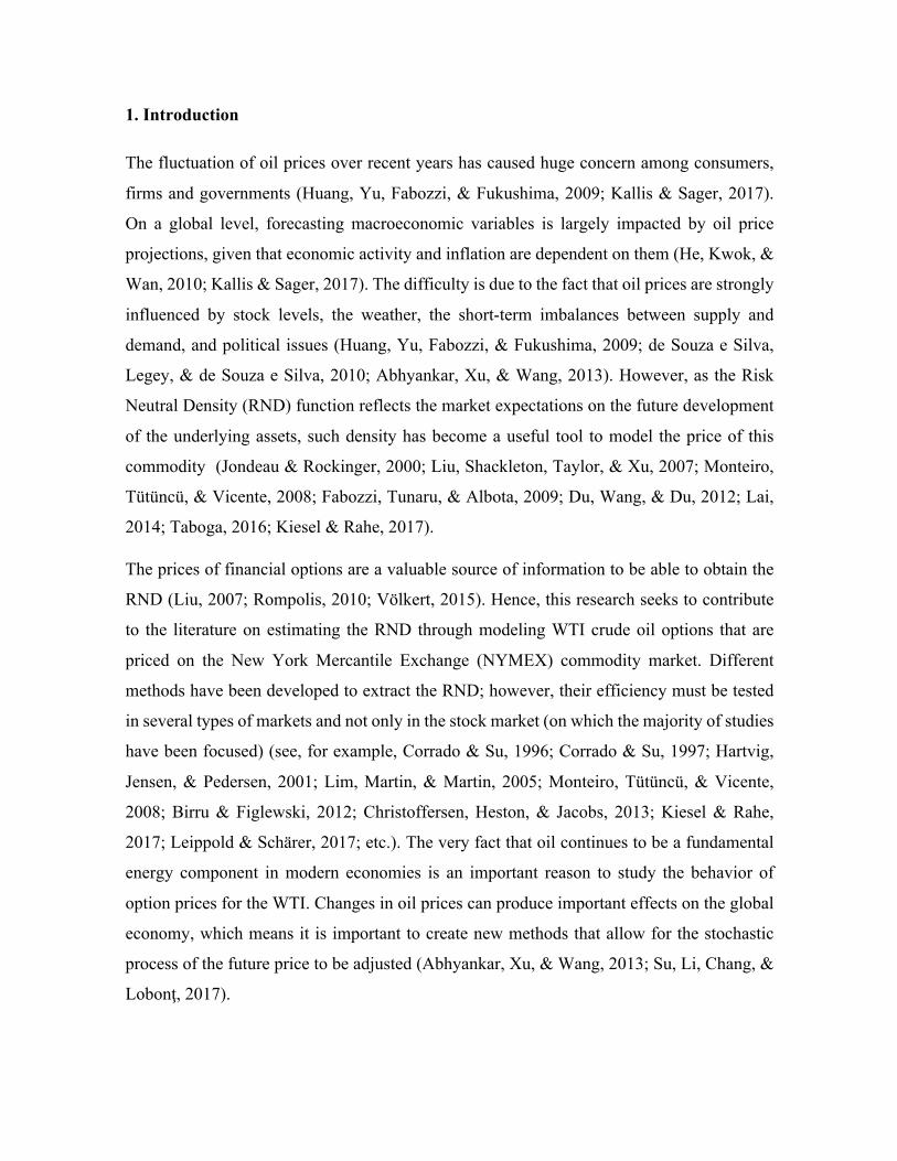
TABLE 2 ESTIMATED PARAMETERS, BLACK-SCHOLES VS. SNP
Date of event
Number of prices
observed
Panel A Black-Scholes Panel B SNP
Implicit standard deviation Implicit standard
deviation Implicit
asymmetry
Implicit excess
kurtosis 20/01/2016 82 0.65 0.70 -0.15 0.08 22/01/2016 82 0.59 0.61 -0.05 0.07 27/01/2016 82 0.65 0.68 -0.07 0.06 09/02/2016 63 0.70 0.74 -0.15 0.11 10/03/2016 60 0.49 0.51 -0.14 0.11 11/05/2016 46 0.40 0.41 -0.14 0.08 24/06/2016 57 0.40 0.42 -0.30 0.13 02/08/2016 44 0.44 0.46 -0.17 0.11 18/08/2016 46 0.34 0.35 -0.13 0.07 28/09/2016 94 0.42 0.43 -0.14 0.14 10/10/2016 95 0.35 0.36 -0.16 0.12 09/11/2016 46 0.40 0.41 -0.11 0.06 30/11/2016 44 0.40 0.41 -0.17 0.04 19/01/2017 59 0.29 0.30 -0.16 0.05 24/01/2017 61 0.29 0.30 -0.11 0.03 The table summarizes the results from the estimations made with the Black-Scholes model and the SNP option pricing model. The first column shows each one of the dates selected in the study, and the second column contains the number of market prices observed in each date. Panel A shows the implicit standard deviation, the implicit skewness, and the implicit excess kurtosis for the SNP model.
The results show very close implicit standard deviations. However, as shown in Panel B, the
results suggest that the implicit distributions are leptokurtic and negatively biased. These
findings are consistent with those obtained by Corrado & Su (1996), Backus, Foresi, Li, &
Wu (1997), Corrado & Su (1997) and Nikkinen (2003). Also, they strengthen existing
evidence on the behavior of returns and underlying asset prices, which usually do not present
normal and lognormal behavior, respectively (MacBeth & Merville, 1979).
Based on the input parameters presented in Table 2, the theoretical price was obtained for the
call options for each one of the dates selected in the study. Using Table 3, it is possible to
compare the average market price observed with the average theoretical price under a
lognormal RND (see panel A) and a log-SNP RND (see panel B).

TABLE 3 COMPARISON OF THE AVERAGE MARKET PRICE FOR THE CALL OPTIONS VS. THE THEORETICAL PRICE
Date of event
Number of prices
observed
Average call option market
price ($US)
Panel A Lognormal Panel B Log-SNP
Average call option theoretical price ($US)
Difference in average
market and theoretical call option price ($US)
Average call option theoretical price ($US)
Difference in average
market and theoretical call option price ($US)
20/01/2016 82 0.507 0.501 0.005 0.504 0.003
22/01/2016 82 1.203 1.188 0.015 1.200 0.003
27/01/2016 82 1.221 1.206 0.014 1.218 0.002
09/02/2016 63 1.156 1.145 0.010 1.155 0.000
10/03/2016 60 3.984 3.965 0.019 3.982 0.002
11/05/2016 46 6.940 6.912 0.028 6.938 0.002
24/06/2016 57 6.411 6.371 0.040 6.408 0.003
02/08/2016 44 1.829 1.832 -0.003 1.827 0.002
18/08/2016 46 5.551 5.532 0.019 5.548 0.003
28/09/2016 94 3.834 3.820 0.013 3.832 0.002
10/10/2016 95 5.275 5.259 0.015 5.271 0.003
09/11/2016 46 2.515 2.514 0.001 2.514 0.001
30/11/2016 44 4.227 4.219 0.008 4.226 0.000
19/01/2017 59 4.862 4.855 0.007 4.859 0.003
24/01/2017 61 5.238 5.231 0.007 5.235 0.003 The table compares the average price observed on the market with the average theoretical price. The first column shows each one of the dates selected in the study, the second column shows the number of market prices observed, and the third shows the average market price on each date selected in the study. Panel A shows the average theoretical price that follows a lognormal RND. Panel B shows the average theoretical price that follows a log-SNP RND.
When comparing the average market prices and the average theoretical prices for each one
of the distributions, we found that if the prices follow a lognormal RND, they tend to
statistically underestimate the call options prices. Particularly, for May 11 and June 24 2016
when the option averages were more in the money, the difference was more noticeable. This
result is not surprising given that Rubinstein (1994) obtained this empirical regularity for
options on the S&P500 index.
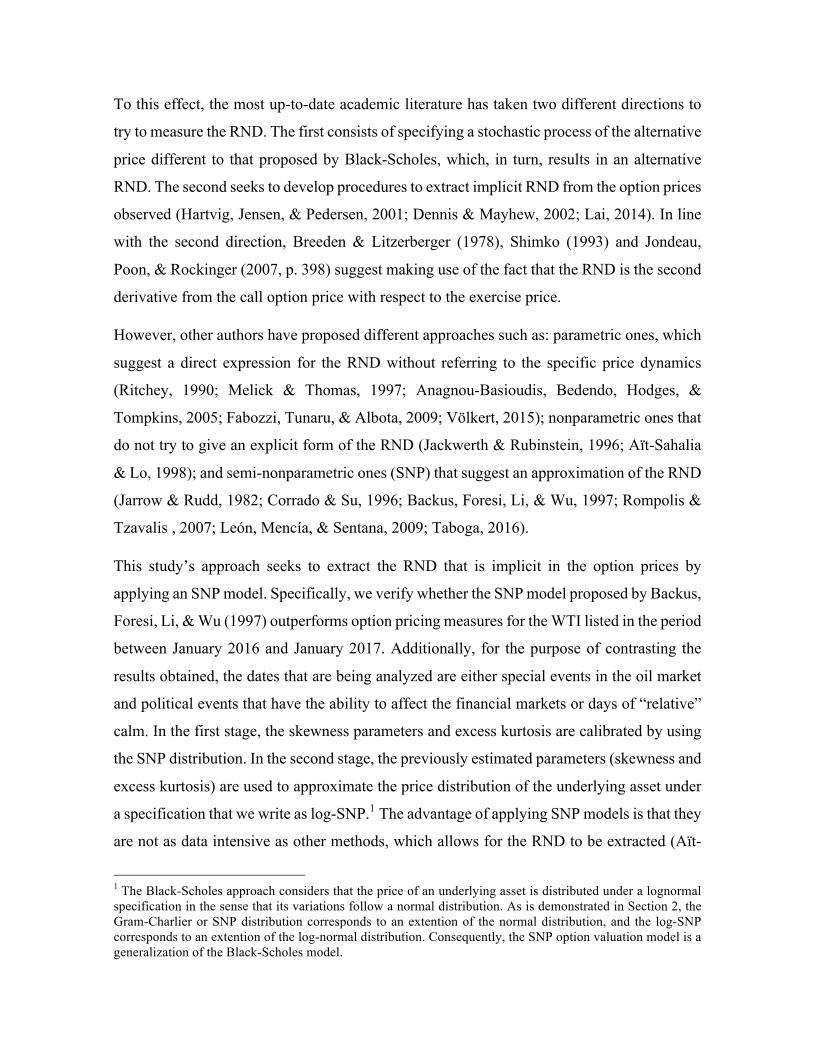
FIGURE 2 RISK NEUTRAL DENSITY
The figure shows the risk neutral density (RND) function for January 24 2017, a day of relative calm (Calm) in the financial markets. The grey line corresponds to the lognormal specification and the black line corresponds to a Log-SNP specification.
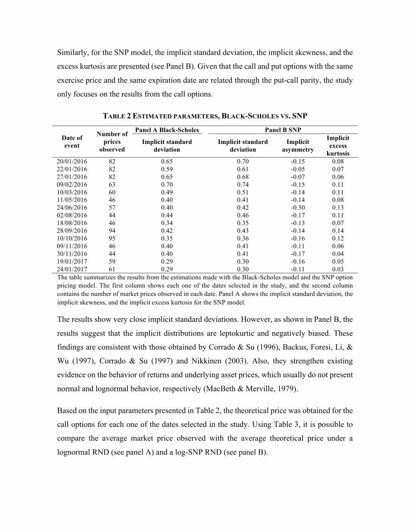
FIGURE 3 RISK NEUTRAL DENSITY
The figure shows the risk neutral density (RND) function for June 24 2016, a day on which news events (News) affected the financial markets. The grey line corresponds to the lognormal specification and the black line corresponds to a Log-SNP specification.
An example of the lognormal - equation (12) - and log-SNP - equation (13) - RNDs are
shown in Figures 2 and 3. We (randomly) selected one of the dates of relative calm and one
of the dates on which there was an event that affected the behavior of the WTI. The first
corresponds to January 24 2017 (Figure 2). The second date corresponds to June 24 2016, a
day on which the financial markets reacted adversely due to the British voting in favor of
leaving the European Union (Figure 3). Note that for the date of relative calm (Calm), the

RNDs under both specifications do not seem very different. However, for the second date
(News), the RND that follows the log-SNP distribution is more biased than the lognormal
one. This seems to allow a better collection of the evolution of the option prices.
In addition to the monetary difference between the average market and theoretical prices,
shown in Table 3, as a measure of goodness of fit, the mean absolute value (MAE) of the
residuals is calculated as explained in subsection 2.2. As shown in Table 4, for all the dates
in the study, the prices that follow a log-SNP RND consistently have a lower MAE.
TABLE 4 MEAN ABSOLUTE ERROR OF THE RESIDUALS, LOGNORMAL VS. LOG-SNP
Date of event
Lognormal Log-SNP Mean absolute error Mean absolute error
20/01/2016 0.0204 0.0051 22/01/2016 0.0165 0.0039 27/01/2016 0.0186 0.0039 09/02/2016 0.0342 0.0033 10/03/2016 0.0449 0.0068 11/05/2016 0.0516 0.0061 24/06/2016 0.1076 0.0186 02/08/2016 0.0397 0.0103 18/08/2016 0.0445 0.0067 28/09/2016 0.0478 0.0090 10/10/2016 0.0451 0.0076 09/11/2016 0.0326 0.0076 30/11/2016 0.0464 0.0091 19/01/2017 0.0458 0.0080 24/01/2017 0.0304 0.0079
The table shows the mean absolute error (MAE) of the residuals when estimating call option prices. The first column shows each of the dates selected in the study. The second column shows the MAE under a lognormal specification, and the third column shows the MAE under a log-SNP specification.

FIGURE 4 MEAN ABSOLUTE ERROR OF THE RESIDUALS
The figure shows the mean absolute error (MAE) when estimating call option prices on January 24 2017, a day of relative calm (Calm) in financial markets. The figure on the left corresponds to the MAE under a lognormal specification, and the figure on the right corresponds to the MAE under a log-SNP specification.
FIGURE 5 MEAN ABSOLUTE VALUE OF THE RESIDUALS
The figure shows the mean error of the absolute value of the residuals (MAE) when estimating call option prices on June 24 2016, a day on which the news affected financial markets. The figure on the left corresponds to the MAE under a lognormal specification, and the figure on the right corresponds to the MAE under a log-SNP specification.

Figures 4 and 5 graphically support the results presented in Table 4. Specifically, they offer
an example for the same dates of calm (Figure 4) and news events in the market (Figure 5)
that were previously selected. The main difference between the modeled RNDs is the ability
to capture the high-order moments such as skewness and excess kurtosis. Especially for the
dates on which there was the most amount of market uncertainty, the results suggest a better
adjustment for the prices from the log-SNP distribution.
Studying models that allow for a better fit to be obtained between the market prices and the
theoretical prices is fundamental, not only from an option pricing point of view but also from
a risk management perspective. For example, within risk management framework one of the
most important issues is quantifying the change in the option price relatively to the change
in the price of an underlying asset (Backus, Foresi, Li, & Wu, 1997).
In this case, as a hedging strategy against risk, the calculation of measurements such as the
option’s delta becomes crucial. This measurement quantifies the sensitivity of the option
price in response to a change in the price of the underlying asset. With the Black-Scholes
model, we can demonstrate that the delta (Δ"#) is given by Δ%&''"# = Φ *+ for the call option,
and by Δ,-."# = Φ *+ − 1 for the put option (see the proof in Appendix A).
However, as we have previously shown, the results obtained in Table 2 suggest that the
implicit distributions in the option prices are leptokurtic and negatively biased. As such, it is
necessary that the delta also captures the effects of the skewness and the excess kurtosis. In
this case, the delta of the SNP model is given by:
Δ%&''#12 = Φ *+ −34
5∅ *+ 1 − *+
7 + 3*+: ; − 2:7; +
=>∅ *+ 3*+ 1 − 2:7; − *+
? + 4*+7: ; − 4: ; + 3:?;
?7 , (14)
for the call option, and by
Δ,-.#12 =A2BCD
A#E− 1 (15)
for the put option (see the proof in Appendix B).
As shown in the previous equations, the traditional Black-Scholes approximation, which is
frequently used in risk hedging and management of options, can differ substantially when the
option price shows skewness and excess kurtosis. Consequently, it is possible to reach
incorrect hedging decisions that lead to severe losses.
5. Conclusions
This study uses the SNP model proposed by Backus, Foresi, Li, & Wu (1997) who follow a
Gram-Charlier A series expansion around the normal density function. The Black-Scholes
model, which is a universal standard used in valuing options, was used as the benchmark.
Using options prices for WTI crude oil traded on NYMEX in the period between January
2016 and January 2017, the skewness and excess kurtosis parameters were calibrated by
using the SNP distribution. Compared to a normal distribution, a negative skewness was
found, as well as a positive excess of kurtosis. These results were constant for the ten dates
that were selected taking into account either special events in the oil market or political events
that could affect financial markets and five days of relative calm.
Furthermore, when the average market price is observed in comparison to the average
theoretical price, we found that the option prices under a lognormal RND tend to
systematically be underestimated. This result is even more remarkable on the dates during
which the financial markets are more unstable. In summary, we can conclude that the log-
SNP RND option pricing model outperforms the traditional Black-Scholes model when
pricing WTI options. These significant gains in accuracy are due to the fact that the terms
accounting for skewness and excess kurtosis seem to be a relevant source of information,
particularly on the presence of extreme events. Therefore the log-SNP model should be
implemented for undertaking appropriate risk hedging and management strategies.
Acknowledgements
We thank financial support from the Spanish Ministry of Economics and Competitiveness
[project ECO2016-75631-P], Junta de Castilla y León [project SA072U16], FAPA-Uniandes
[project P16.100322.001] and Universidad EAFIT.
References
Abhyankar, A., Xu, B., & Wang, J. (2013). Oil price shocks and the stock market: evidence from Japan. The Energy Journal, 34(2), 199-222.
Aït-Sahalia, Y., & Lo, A. W. (1998). Nonparametric estimation of state-price densities implicit in financial asset prices. The Journal of Finance, 53(2), 499–547.
Anagnou-Basioudis, I., Bedendo, M., Hodges, S. D., & Tompkins, R. (2005). Forecasting accuracy of implied and GARCH-based probability density functions. Review of Futures Markets 11(1), 41-66.
Antonakakis, N., Chatziantoniou, I., & Filis, G. (2017). Oil shocks and stock markets: dynamic connectedness under the prism of recent geopolitical and economic unrest. International Review of Financial Analysis, 50, 1-26.
Backus, D., Foresi, S., Li, K., & Wu, L. (1997). Accounting for Biases in Black-Scholes. Manuscript, The Stern School at New York University, 1-46.
Birru, J., & Figlewski, S. (2012). Anatomy of a meltdown: the risk neutral density for the S&P 500 in the fall of 2008. Journal of Financial Markets, 15(2), 151-180.
Black, F., & Scholes, M. (1973). The pricing of options and corporate liabilities. Journal of Political Economy, 81(3), 637–659.
Breeden, D., & Litzerberger, R. (1978). Prices of state-contingent claims implicit in options prices. Journal of Business, 51(4), 621–651.
Brown, C. A., & Robinson, D. M. (2002). Skewness and kurtosis implied by option prices: a correction. The Journal of Financial Research, 25(2), 279–282.
Christoffersen, P. (2012). Elements of financial risk management (2nd ed.). Waltham: Academic Press.
Christoffersen, P., Heston, S., & Jacobs, K. (2013). Capturing option anomalies with a variance-dependent pricing kernel. Review of Financial Studies, 26(8), 1963-2006.
Corrado, C. J., & Su, T. (1996). Skewness and kurtosis in S&P 500 index returns implied by option prices. The Journal of Financial Research, 19(2), 175-192.

Corrado, C. J., & Su, T. (1997). Implied volatility skews and stock return skewness and kurtosis implied by stock option prices. The European Journal of Finance, 3(1), 73–85.
Cortés, L. M., Mora-Valencia, A., & Perote, J. (2016). The productivity of top researchers: a semi-nonparametric approach. Scientometrics, 109(2), 891-915.
Cortés, L. M., Mora-Valencia, A., & Perote, J. (2017). Measuring firm size distribution with semi-nonparametric densities. Physica A, Statisctical Mechanics and its Applications, 485, 35-47.
Das, S. R., & Sundaram, R. K. (1999). Of smiles and smirks: a term structure perspective. The Journal of Financial and Quantitative Analysis, 34(2), 211-239.
de Souza e Silva, E. A., Legey, L. F., & de Souza e Silva, E. A. (2010). Forecasting oil price trends using wavelets and hidden Markov models. Energy Economics, 32(6), 1507-1519.
Dennis, P., & Mayhew, S. (2002). Risk-neutral skewness: evidence from stock options. Journal of Financial and Quantitative Analysis, 37(3), 471–493.
Du, Y., Wang, C., & Du, Y. (2012). Inversion of option prices for implied risk-neutral probability density functions: general theory and its applications to the natural gas market. Quantitative Finance, 12(12), 1877-1891.
Fabozzi, F. J., Tunaru, R., & Albota, G. (2009). Estimating risk-neutral density with parametric models in interest rate markets. Quantitative Finance, 9(1), 55-70.
Fama, E. (1965). The behaviour of stock market prices. Journal of Business, 38(1), 34–105.
Feng, P., & Dang, C. (2016). Shape constrained risk-neutral density estimation by support vector regression. Information Sciences, 333(C), 1-9.
Friesen, G., Zhang, Y., & Zorn, T. (2012). Heterogeneous beliefs and risk-neutral skewness. Journal of Financial and Quantitative Analysis, 47(4), 851-872.
Fusai, G., & Roncoroni, A. (2008). Implementing models in quantitative finance (1st ed.). Berlin: Springer.
Hartvig, N. V., Jensen, J. L., & Pedersen, J. (2001). A class of risk neutral densities with heavy tails. Finance and Stochastics, 5(1), 115-128.
He, A., Kwok, J., & Wan, A. (2010). An empirical model of daily highs and lows of West Texas Intermediate crude oil prices. Energy Economics, 32(6), 1499-1506.
Huang, D., Yu, B., Fabozzi, F., & Fukushima, M. (2009). CAViaR-based forecast for oil price risk. Energy Economics, 31(4), 511-518.
Jackwerth, J., & Rubinstein, M. (1996). Recovering probability distributions from options prices. Journal of Finance, 51(5), 1611–1631.

Jarrow, R., & Rudd, A. (1982). Approximate option valuation for arbitrary stochastic processes. Journal of Financial Economics,10(3), 347-369.
Jondeau, E., & Rockinger, M. (2000). Reading the smile: the message conveyed by methods which infer risk neutral densities. Journal of International Money and Finance, 19(6), 885–915.
Jondeau, E., Poon, S.-H., & Rockinger, M. (2007). Financial Modeling Under Non-Gaussian Distributions. London: Springer.
Kallis, G., & Sager, J. (2017). Oil and the economy: a systematic review of the literature for ecological economists. Ecological Economics, 131, 561-571.
Kiesel, R., & Rahe, F. (2017). Option pricing under time-varying risk-aversion with applications to risk forecasting. Journal Of Banking & Finance, 76(C), 120-138.
Lai, W.-N. (2014). Comparison of methods to estimate option implied risk-neutral densities. Quantitative Finance, 14(10), 1839-1855.
Leippold, M., & Schärer, S. (2017). Discrete-time option pricing with stochastic liquidity. Journal of Banking & Finance, 75, 1-16.
León, A., Mencía, J., & Sentana, E. (2009). Parametric properties of semi-nonparametric distributions, with applications to option valuation. Journal of Business & Economic Statistics, 27( 2), 176-192.
Lim, G. C., Martin, G. M., & Martin, V. L. (2005). Parametric pricing of higher order moments in S&P500 options. Journal of Applied Econometrics,20(3), 377–404.
Liu, X. (2007). Bid–ask spread, strike prices and risk-neutral densities. Applied Financial Economics, 17(11), 887–900.
Liu, X., Shackleton, M. B., Taylor, S. J., & Xu, X. (2007). Closed-form transformations from risk-neutral to real-world distributions. Journal of Banking & Finance, 31(5), 1501-1520.
MacBeth, J., & Merville, L. (1979). An empirical examination of the Black-Scholes call option pricing model. Journal of Finance, 34(5), 1173-1186.
Melick, W. R., & Thomas, C. P. (1997). Recovering an asset’s implied PDF from option prices: an application to crude oil during the Gulf crisis. Journal of Financial and Quantitative Analysis, 32(1), 91–115.
Monteiro, A. M., Tütüncü, R. H., & Vicente, L. N. (2008). Recovering risk-neutral probability density functions from options prices using cubic splines and ensuring nonnegativity. European Journal of Operational Research, 187(2), 525-542.
Nikkinen, J. (2003). Normality tests of option-implied risk-neutral densities: evidence from the small Finnish market. International Review of Financial Analysis, 12(2), 99–116.

Ñíguez, T-M., Paya, I., Peel, D., & Perote, J. (2012). On the stability of the constant relative risk aversion (CRRA) utility under high degrees of uncertainty. Economics Letters, 115(2), 244-248.
Peña, I., Rubio, G., & Serna, G. (1999). Why do we smile? On the determinants of the implied volatility function. Journal of Banking & Finance, 23(8), 1151 – 1179.
Postali, F., & Picchetti, P. (2006). Geometric Brownian Motion and structural breaks in oil prices: a quantitative analysis. Energy Economics, 28(4), 506-522.
Ritchey, R. (1990). Call option valuation for discrete normal mixtures. Journal of Financial Research, 13(4), 285–296.
Rompolis, L. S. (2010). Retrieving risk neutral densities from European option prices based on the principle of maximum entropy. Journal of Empirical Finance, 17(5), 918-937.
Rompolis, L. S., & Tzavalis , E. (2007). Retrieving risk neutral densities based on risk neutral moments through a Gram–Charlier series expansion. Mathematical and Computer Modelling, 46(1–2), 225-234.
Rubinstein, M. (1994). Implied binomial trees. The Journal of Finance, 49(3), 771-818.
Shimko, D. (1993). Bounds of Probability. RISK Magazine, 6, 33-37.
Su, C., Li, Z., Chang, H., & Lobonţ, O. (2017). When will occur the crude oil bubbles? Energy Policy, 102, 1-6.
Taboga, M. (2016). Option-implied probability distributions: How reliable? How jagged? International Review Of Economics & Finance, 45, 453-469.
Völkert, C. (2015). The distribution of uncertainty: evidence from the VIX options market. Journal of Futures Markets, 35(7), 597-624.

Appendix A
This appendix derives the expression for the delta of the Black-Scholes model (Δ"#):
From equation (4) we know that the theoretical price for the Black-Scholes call option can
be obtained as
F"# G; I = JKL *+ − GMNO5L *7 ,
where L *+ =+
7PMQRS
S *TUVNW
y L *7 =+
7PMQRS
S *TUSNW
is the cdf of the normal
standard distribution, *+ ='Y #E Z [ O[\S 7 5
\ 5 and *7 = *+ − : ;.
First, it is estimated that
A](UV)
AUV=
+
7PMQ_V
S
S , (A.1)
A](US)
AUS=
+
7PMQ_S
S
S ,
=+
7PMQ _VQa b
S
S .
Developing the squared binomial and replacing*+ , the following can be obtained
+
7PMQ_V
S
S Mcd BE e f gfaS S b a b
a b MaSbS , from which
A](US)
AUS=
+
7PMQ_S
S
S#E
ZMO5. (A.2)
Also, the following holds true,
AUV
A#E=
AUS
A#E=
+
#E\ 5. (A.3)
The delta of an option is defined as the partial derivative of the option price with respect to
the price of the underlying asset, for the call

Δ%&''"# =
AhiB
A#E.
AhiB
A#E= Φ *+ + JK
A](UV)
A#E− GMO5
A] US
A#E,
= Φ *+ + JKA](UV)
AUV
AUV
A#E− GMO5
A](US)
AUS
AUS
A#E,
replacing equations (A.1), (A.2) and (A.3), the following is obtained
Δ%&''"# = Φ *+ . □ (A.4)
For the put option, it can be demonstrated that,
Δ,-."# = Φ *+ − 1. (A.5)
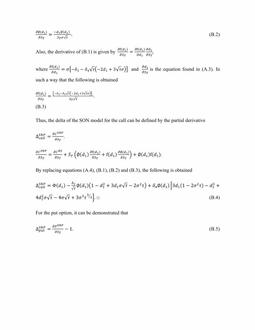
Appendix B
This appendix derives the expression for the delta of the SNP (Δ#12) model:
From equation (5), we know that the theoretical price for the SNP call option can be obtained
as
F#12 G; I = F"# G; I + JKk *+ l *+ ,
with l *+ = : =? 2 ;: − *+ − => ; 1 − *+7 + 3*+ ;: − 3;:7 , (B.1)
where k *+ =+
7PMQ_V
S
S is the pdf of the normal standard distribution, and *+ =
'Y #E Z [ O[\S 7 5
\ 5.
First, the following are derived,
A∅(UV)
A#E=
A∅(UV)
AUV
AUV
A#E,
where A∅(UV)AUV
= −*+∅ *+ y AUVA#E
is the equation found in (A.3). Also, the following is
obtained
A∅(UV)
A#E=
NUV∅ UV
#E\ 5. (B.2)
Also, the derivative of (B.1) is given byAm(UV)A#E
=Am(UV)
AUV
AUV
A#E,
where Am(UV)AUV
= : −=3 − =4 ; −2*1 + 3 ;: and AUVA#E
is the equation found in (A.3). In
such a way that the following is obtained
Am(UV)
A#E=
−=3−=4 ; −2*1+3 ;:
#E 5.
(B.3)
Thus, the delta of the SON model for the call can be defined by the partial derivative
Δ%&''#12 =
AhBCD
A#E.
AhBCD
A#E=
AhiB
A#E+ JK ∅ *+
Am(UV)
A#E+ f(*+)
A∅(UV)
A#E+ ∅ *+ f(*+).
By replacing equations (A.4), (B.1), (B.2) and (B.3), the following is obtained
Δ%&''#12 = Φ *+ −
34
5∅ *+ 1 − *+
7 + 3*+: ; − 2:7; + =>∅ *+ 3*+ 1 − 2:7; − *+
? +
4*+7: ; − 4: ; + 3:?;
?7 . □ (B.4)
For the put option, it can be demonstrated that
Δ,-.#12 =
A2BCD
A#E− 1. (B.5)