copyright by george phillip purcell, jr. 2015

Copyright

by

George Phillip Purcell, Jr.

2015

The Dissertation Committee for George Phillip Purcell, Jr. Certifies that this is the

approved version of the following dissertation:

An Econometric Estimate of Baumol and Bowen Expenditures at Texas

Public Universities Following Tuition Deregulation

Committee:

Patricia Somers, Supervisor

Jason Abrevaya

James Cofer

Richard Reddick

Edwin Sharpe

An Econometric Estimate of Baumol and Bowen Expenditures at Texas


by

George Phillip Purcell, Jr., B.S., M.P.Aff.

Dissertation

Presented to the Faculty of the Graduate School of

The University of Texas at Austin

in Partial Fulfillment

of the Requirements

for the Degree of

Doctor of Philosophy

The University of Texas at Austin

May 2015

Dedication

To my son, Graham.

v

Acknowledgements

This research would not exist without the direct involvement of three professors at

UT Austin. John Higley recruited me into the Government department. From him I

learned the key theoretical perspective on public policy that I use virtually every day (and

I hope that completing this Ph.D. may go some small way to alleviating his

disappointment in me). William Lasher gave me a second shot by facilitating my transfer

into Educational Administration and fought to ensure my previous coursework made a

part-time Ph.D. goal realistic. His course in the finance of higher education was

foundational to my work in this study. Pat Somers recognized that I was struggling with

an impossible research topic. She intervened and turned me back around to my interest in

starting the program in the first place—understanding why college costs so much (and

why it keeps costing more). She kept me on the path to completion on times when I was

wavering. Without her, I would not have finished.

I would like to thank the members of this dissertation committee. Jason

Abrevaya, for lending his insights into the econometric modeling and being gentle to a

novice in his field. James Cofer, for providing the perspective of a leader who had to

struggle with the consequences of choices that the data in this research record. Edwin

Sharpe, for his deep understanding of Texas policy and politics—and for being one of the

most decent human beings I have ever met. Richard Reddick, for coming in as an All

Star pinch hitter and for a wonderful course on the history of higher education.

Finally, I would like to acknowledge the love and support of my wife, Kenzie,

while I pursued this degree and to celebrate the life of the best animal friend I will ever

have: Lone Star the Cat. I miss you, buddy.

vi

An Econometric Analysis of Baumol and Bowen Expenditures at Texas


George Phillip Purcell, Jr., Ph.D.

The University of Texas at Austin, 2015

Supervisor: Patricia Somers

Expenditures per FTE student have risen rapidly in real terms in public higher

education in the United States for over three decades. Two theory-grounded hypotheses

have been advanced to explain this growth. Baumol’s (1966) “cost disease” argument is

a macroeconomic perspective arguing that industries heavily reliant on skilled labor have

limited ability to increase productivity but must increase their wage rate above their

productivity gains to compete for this skilled labor in the labor market. Bowen’s (1980)

“revenue theory of costs” proposes a microeconomic explanation that universities raise

all they can and spend all they raise. Bowen’s thesis has been expanded into a behavioral

theory by Martin (2011), who argues that the nexus of non-profit status, principal-agent

confusion, and prestige seeking behavior are responsible for increased expenditures.

Following Martin and Hill (2012), this study presents an econometric model that

allocates expenditures to these two theoretical perspectives.

Statewide real average expenditures per FTE student at Texas public universities

increased 9% from fiscal year 2003 to fiscal year 2011 following tuition deregulation.

Analysis of yearly fixed effects suggests that this policy change led to an increase in real

expenditures above pre-deregulation levels on the order of $1,400 per FTE student. The

vii

ratio of Bowen to Baumol expenses is highest at elite Research universities and is lowest

at the least research intensive Master’s universities.

Additional tuition revenue was associated with a decline of Bowen expenditures

relative to Baumol expenditures at Research institutions of -5% while Emerging Research

and Doctoral institution displayed substantial increases in Bowen expenditures relative to

Baumol expenditures (6% and 4%). This finding suggests that lower-level research

universities with aspirations to higher research intensity increase their proportion of

Bowen expenditures in conditions of expanding revenue. Research universities used

additional revenue to reduce an existing cross-institutional subsidy from graduate

education to the rest of the institution.

Keywords: Texas, econometrics, higher education, tuition deregulation, cost of

higher education

viii

Table of Contents

List of Tables ........................................................................................................ xii

List of Figures ...................................................................................................... xiii

Chapter 1: Introduction ............................................................................................1

Background .....................................................................................................1

Problem Statement ..........................................................................................2

Purpose ............................................................................................................2

Research Questions .........................................................................................3

Significance.....................................................................................................3

Key Elements of Existing Literature ...............................................................4

Method ............................................................................................................5

Assumptions and Limitations .........................................................................5

Scope and Delimitations .................................................................................6

Definitions.......................................................................................................6

Organization of Study .....................................................................................7

Chapter 2: Literature Review ...................................................................................9

Thinking Clearly About “Costs” .....................................................................9

The Baumol Hypothesis: Expenditures Rise Due To Differential Productivity Gains in the Economy ..............................................................11

The Bowen Hypothesis: Expenditures Constrained Only By Revenues ........................................................................................15

Defining Prestige ..........................................................................................20

Comparison of the Hypotheses .....................................................................22

Public Universities and External Cost Control .............................................23

Tuition Deregulation in Texas—A Natural Experiment ...............................24

Summary .......................................................................................................31

Chapter 3: Methods ................................................................................................33

Problem Statement and Research Questions.................................................33

Theoretical Paradigm ....................................................................................34

ix

Procedure ......................................................................................................37

Design ...........................................................................................................37

Source of Data...............................................................................................37

Subjects/Population.......................................................................................37

Variables .......................................................................................................38

Dependent Variable. ............................................................................38

Independent Variables—Enrollments. .................................................39

Independent Variables—Salaries and Benefits. ...................................39

Independent Variables—Faculty Measurements. ................................40

Independent Variables—Staff Measurements. ....................................41

Independent Variables—Revenues. .....................................................41

Independent Variables—Fixed Effects and Controls. .........................41

Apparatus, Instruments, Protocols ................................................................42

Robust Regression Techniques. ...........................................................43

Control Instruments. ............................................................................47

Instruments in the Baumol Decomposition..........................................48

Instruments in the Bowen Decomposition. ..........................................48

Functional Form of Regression Equation .....................................................50

Institutional Review Board Approval ...........................................................52

Chapter 4: Analysis of Changes in Model Variables Over Time ..........................53

Measurement of the Dependent Variable .....................................................53

Measurement of the Independent Variables .................................................55

Measurement of the Independent Variables—Enrollments. ................55

Independent Variables—Salaries and Benefits. ...................................63

Independent Variables—Faculty Measurements. ................................67

Independent Variables—Staff Measurements. ....................................75

Independent Variables—Revenue. ......................................................85

Summary of Changes in the Statewide Variables. ........................................90

Variations at Research Institutions. .....................................................91

Variations at Emerging Research Institutions......................................92

x

Variations at Doctoral Institutions. ......................................................93

Variations at Comprehensive Institutions. ...........................................93

Variations at Master’s Institutions. ......................................................93

Summary of Changes in the Public Higher Education Sector from 2003 to 2011 .............................................................................94

Chapter 5: Econometric Model Results .................................................................96

Problem Statement and Research Questions.................................................96

Presentation of the Regression Models .........................................................97

Estimation of Instrument Effects ................................................................113

Estimating Total Baumol and Bowen Effects .............................................122

Investigating Multicollinearity....................................................................125

Answering the Research Questions ............................................................128

Conclusion ..................................................................................................129

Chapter 6: Summary and Conclusions .................................................................130

Problem Statement, Research Questions, and Methods..............................130

Results .........................................................................................................132

Relationship to Literature ...........................................................................134

Scale Changes. ...................................................................................134

Cost Savings.......................................................................................135

Revenue..............................................................................................136

Productivity. .......................................................................................136

Compensation. ...................................................................................136

Governance. .......................................................................................137

Significance.................................................................................................137

Unexpected and Surprising Findings ..........................................................139

Recommendations for Practice ...................................................................140

Limitations ..................................................................................................141

Implications.................................................................................................141

Future Research ..........................................................................................142

Conclusion ..................................................................................................143

xi

Appendix ..............................................................................................................144

References ............................................................................................................146

Vita .....................................................................................................................153

xii

List of Tables

Table 1: OLS, White (HC), and Newey West (HAC)

Regression Results—Intercept and Control Variables .....................98

Table 2: OLS, Huber (M-Estimator), and Yohai (MM-Estimator)

Regression Results—Intercept and Control Variables ...................101


Regression Results— Scale Changes and Cost Savings .................104


Regression Results—Scale Changes and Cost Savings ..................106


Regression Results—Baumol and Bowen Instruments ...................108


Regression Results—Baumol and Bowen Instruments ...................111

Table 7: Cluster Groupings of Interval-Ratio Variables ..............................126

Table 8: Results for LASSO Regression ........................................................126

xiii

List of Figures

Figure 1. Average real total cost (tc)

at Texas public universities. ..............................................................53

Figure 2. Average real total cost (tc)

at Texas public universities by THECB institution type. .................54

Figure 3. Average FTE student enrollment (ftestu)


Figure 4. Average FTE student enrollment (ftestu)


Figure 5. Average full-time graduate student enrollment (ftgrad)


Figure 6. Average full-time graduate student enrollment (ftgrad)


Figure 7. Average part-time student enrollment (ptstu)


Figure 8. Average part-time student enrollment (ptstu)


Figure 9. Ratio of graduate assistants to FTE students (ta)


Figure 10. Ratio of graduate assistants to FTE students (ta)


Figure 11. Average real staff salaries (staffsal)


xiv

Figure 12. Average real staff salaries (staffsal)


Figure 13. Average real staff benefits (benstaff)


Figure 14. Average real staff benefits (benstaff)


Figure 15. Contract faculty per 100 FTE students (cf)


Figure 16. Contract faculty per 100 FTE students (cf)


Figure 17. Part-time faculty per 100 FTE students (ptf)


Figure 18. Part-time faculty per 100 FTE students (ptf)


Figure 19. FTE faculty per 100 FTE students (ftef)


Figure 20. FTE faculty per 100 FTE students (ftef)


Figure 21. Tenure-track faculty per professional non-academic staff (ttad)


Figure 22. Tenure-track faculty per professional non-academic staff (ttad)


Figure 23. Non-professional FTE staff

per 100 FTE students (ftenpro) at Texas public universities. ...........75

xv

Figure 24. Non-professional FTE staff

per 100 FTE students (ftenpro) at Texas public universities

by THECB institution type. ..............................................................76

Figure 25. Executive and professional FTE staff

per 100 FTE students (fteadmin) at Texas public universities. .........77

Figure 26. Executive and professional FTE staff

per 100 FTE students (fteadmin) at Texas public universities. .........78

Figure 27. FTE staff per FTE executives (staffsize)


Figure 28. FTE staff per FTE executives (staffsize)


Figure 29. Part-time executive and professional staff

per 100 FTE students (ptadmin) at Texas public universities. ..........81

Figure 30. Part-time executive and professional staff

per 100 FTE students (ptadmin) at Texas public universities


Figure 31. Part-time non-professional staff

per 100 FTE students (ptnpro) at Texas public universities. ............83

Figure 32. Part-time non-professional staff

per 100 FTE students (ptnpro) at Texas public universities


Figure 33. Total real revenue per FTE student, less investment income (rev)


Figure 34. Total real revenue per FTE student, less investment income (rev)


xvi

Figure 35. Real other revenue per FTE student, less investment revenue (other)


Figure 36. Real other revenue per FTE student, less interest (other)


Figure 37. Real investment revenue per FTE student (invest)


Figure 38. Real investment revenue per FTE student (invest)


Figure 39. Estimated real expenditure change per FTE student

by fiscal year, controlling for other variables. ................................115

Figure 40. Estimated real expenditure changes per FTE Student due to

Scale Changes by THECB institution type. ....................................116

Figure 41. Estimated real expenditure changes per FTE student due to

Cost Savings by THECB institution type. ......................................117

Figure 42. Estimated expenditure changes per FTE student due to

Compensation by THECB institution type. ....................................119

Figure 43. Estimated real expenditure changes per FTE student due to

Revenue by THECB institution type. .............................................120

Figure 44: Estimated real expenditure changes per FTE student due to

Productivity by THECB institution type.........................................121


Governance by THECB institution type. ........................................122

Figure 46: Estimated real expenditure changes due to

Bowen effects..................................................................................123

xvii


Baumol effects. ...............................................................................123

Figure 48. Bowen-to-Baumol ratio......................................................................124

1

Chapter 1: Introduction

Colleges and universities today spend larger sums in real terms on a per student

basis than at any previous time in American history. This study is motivated by a simple

question: Why has this spending increase occurred? To answer this question, I examine a

natural experiment—the deregulation of tuition in Texas in 2003—when a set of public

higher education institutions in a restricted spending environment were, overnight, turned

into institutions able to price their education services at essentially any level the market

would support. Observing changes in expenditures at these institutions provides insights

into the decision-making that occurred when they were able to access an expanded source

of income. Were these institutions constrained by economic forces beyond their control,

with increased funds used to address systemic labor market issues? Or were they able to

direct new expenditures toward focused areas of their institutions to achieve specific

goals? Understanding the degree of agency institutions possess about expenditure

decisions is critical to developing policy recommendations about the finance of public

higher education.

BACKGROUND

The decreasing affordability of higher education has been an issue of scholarly

interest for many years (Heller, 2001; Mumper, 2003) and has been identified as one of

the key areas of recent scholarly work by Conner and Rabovsky (2011). Students have

taken on an increasingly large share of the costs of operating public higher education.

Between 2005 and 2010, for example, net per student tuition increased both in dollars

(from $7,116 to $8,611) as well as in percentage of operating revenues (21% to 24% ) at

public research institutions (Kirshstein & Hurlburt, 2012). The increasing role student

tuition plays in funding university operations has led to a large increase in the level of

2

student debt over the last ten to fifteen years and there is evidence that this debt, in turn,

constrains the choices of students after college (Rothstein & Rouse, 2010). As costs have

risen, scholars have sought explanations for the phenomena. While some argue that

decreased state appropriations play a key role in the burden taken on by students (Titus,

2009), total expenditures at higher education institutions have risen at a level above the

rate of inflation in the overall economy.

Texas historically had tight Legislative control over institutional tuition and this

control provided a check to growth in institutional expenditures. Following tuition

deregulation in 2003, however, this tight control was removed. As a result, Texas

provides a natural experiment to examine how expenditures change when constrained

higher educational institutions are given the chance to increase real expenditures.

PROBLEM STATEMENT

National per student spending at public, four-year institutions has increased

rapidly in the last three decades and dramatic increases in the real level of tuition paid by

students provide most of the additional funds allowing this increase in spending. In

Texas prior to tuition deregulation per student spending was essentially flat. Following

tuition deregulation, real spending per student increased substantially.

PURPOSE

The research presented in this study uses the Texas case to demonstrate how

universities allocate increases in expenditures—specifically whether those choices are

constrained by macroeconomic factors in the general labor market (the Baumol

hypothesis) or whether unresolved agency problems, the pursuit of institutional interests,

and other microeconomic forces instead explain expenditure decisions (the Bowen

3

hypothesis). This research develops an econometric model of institutional spending

patterns both before and after tuition deregulation.

RESEARCH QUESTIONS

Question 1: To what degree do the competing Baumol and Bowen hypotheses

explain expenditure changes at public four-year institutions of higher education?

Question 2: Do public, four-year institutions of higher education with

strongly defined research missions exhibit different choices in expending these new

funds?

SIGNIFICANCE

Both the Baumol and Bowen hypotheses contain elements of truth. What is most

significant about this study is measuring, in a natural experiment, the relative importance

of the two explanations of increased spending in higher education and how those

expenditures change. This study also represents the first analysis that examines how

these two explanations for expenditures are related to the level of research-intensity of

the institution. While this research is not an evaluation of potential policy responses,

understanding the forces that are increasing spending at public four-year universities is

critical to addressing the challenges that are caused by these increases. To the extent, for

example, that the Baumol hypothesis accounts for expenditures it is likely that the entire

project of mass higher education as currently conceived is unsustainable and that

fundamental changes in the delivery of education to post-secondary students must occur.

On the other hand, to the extent that there are firm-level incentives pushing expenditures

higher at universities, it is possible that regulation, control, and oversight of public higher

education institutions could play an important role in shaping those incentives and in

constraining the growth of these expenditures.

4

KEY ELEMENTS OF EXISTING L ITERATURE

The explanation for rising costs in higher education with the longest intellectual

history is the Baumol hypothesis, often referred to as the “cost disease.” The basic

argument of the Baumol hypothesis is that technological improvements increase

productivity and wages in the general economy, particularly among capital-intensive

“progressive” industries. Labor-intensive “stagnant” industries are not able to achieve

the same level of productivity gains as capital-intensive industries but must still pay

market-level labor rates or lose employees to progressive sectors of the economy. Absent

qualitative changes in technology that increase labor productivity in stagnant sectors the

cost of providing these labor-intensive services will thus increase more rapidly than

general inflation in the economy (Baumol & Bowen, 1966).1

An alternative explanation for the increase in higher education expenditures above

the general rise of prices in the economy is provided by H. R. Bowen (1980). Bowen

studied cross-sectional expenditure data for public and private institutions. He finds that

there is a great divergence in per-student expenditures at universities and concludes that

there is no external pressure enforcing standardized expenditure patterns on these

institutions. In particular there is no external pressure to lower costs because universities

are shielded from competition by geographic location and service differentiation. He

concludes that what institutions categorized as needs “are arguments in favor of increased

funding, not causes of increased costs” (H. R. Bowen, 1980, p. 16). He also points out

that efforts to increase efficiency will not reduce “costs” but simply lead to a reallocation

of spending. In his view, only reductions in revenue can lead to reduced expenditures.

1 The initial work that developed this literature was written by William Baumol and William Bowen. The main competing theory to this approach, to be covered, was developed by the unrelated Howard Bowen.

5

Martin (2011) develops a behavioral framework to ground the Bowen hypothesis

in economic theory. There are three main elements in his framework. First, the pursuit

of prestige occurs because higher education is an “experience good”; consumers of the

good determine its quality by “experiencing” it as opposed to testing various suppliers of

the good through a search procedure (Nelson, 1970). Second, the constant activity of

fund raising in higher education creates a “principal-agent problem” (Martin, 2011, p.

162). Third, the non-profit status of higher education institutions magnifies this

principal-agent problem. In a for-profit enterprise, there is a clear line of control from the

property holders (principals) to their agents (the employees of the firm) through fractional

ownership. In a non-profit, however, there is no discrete ownership interest among the

principals, whose property rights are held in common. Most important, however, is the

fact that any financial residual produced by the non-profit firm is spent within the

institution on staff and not distributed to shareholders as dividends.

METHOD

This study employs an established econometric methodology to construct

regression models that link total per FTE student expenditures to a set of theoretical and

control variables. Using the technique of partial derivatives, estimates of constant dollar

yearly per student expenditures at Texas public universities are divided into amounts

proportionally explained by the Baumol hypothesis, the Bowen hypothesis, and control

instruments.

ASSUMPTIONS AND L IMITATIONS

The primary limitations imposed on this study involve the disaggregation of

employment data available through the federal IPEDS system. While expenditure data in

IPEDS may be separated by the function of the expenditure (e.g., student services), labor

6

measurements are not similarly differentiated. As a result, the econometric analysis in

this research models all expenditures at institutions, including those expenditures

incurred by auxiliary activities such as residence halls and athletic faculties. Since

auxiliary functions should (theoretically) be self-supporting, an ideal study would remove

these expenditures and labor measurements from consideration of the rest of the

enterprise. It is possible that future studies employing the basic methodology from this

study (but using more detailed state-collected data) could provide more precise modeling

of the determinants of expenditures in the academic functions of the university and

measure cross-subsidization between academic and auxiliary activities.

SCOPE AND DELIMITATIONS

The expenditure data for this study was collected from Texas public, four-year

institutions before and after tuition deregulation in 2003. The results of this model are

only suggestive for public institutions in states where tuition either has been deregulated

for some time or that function in an environment of regulated tuition. In addition, the

results from this analysis have only limited application to understanding expenditures at

private institutions. Finally, this study does not address how the quality of the

educational product produced by increasing real expenditures might improve. For

example, increases in spending on student services might lead to increases in persistence

and graduation through increased student engagement (Tinto, 1987).

DEFINITIONS

• FTE Student: Full Time Equivalent Student. An institution has one FTE student

for every 30 semester credit hours or 24 graduate semester credit hours.

7

• GASB: Government Accounting Standards Board. Promulgates accounting

regulations for governmental entities such as public institutions of higher

education.

• HC: Heteroscedastic-consistent estimate of standard errors.

• HAC: Heteroscedastic and autocorrelation consistent estimate of standard errors.

• IPEDS: Integrated Post-Secondary Education Data System. A federal

clearinghouse of verified and validated comparable data collected at the

institutional level.

• M-estimator: Robust regression technique that adjusts for heteroscedasticity.

• MM-estimator: Robust regression technique that adjusts for heteroscedasticity and

the influence of outliers.

• NACUBO: National Association of College and University Business Officers.

Professional organization that develops accounting categories for higher

education expenditures.

• NCES: National Center for Education Statistics. Federal agency responsible for

managing IPEDS.

• SCH: Semester Credit Hours. One SCH is awarded for attendance in one hour of

classroom instruction over the course of a semester or for out-of-classroom work

judged to be equivalent in content to one Carnegie Unit.

• THECB: Texas Higher Education Coordinating Board. The government agency

charged with oversight of higher education in Texas.

ORGANIZATION OF STUDY

The substantive portion of this study contains four chapters. Chapter 2 reviews

the existing literature on costs in higher education and presents a legislative history of

8

tuition deregulation in Texas. Chapter 3 describes the econometric methodology used in

this research. Chapter 4 presents a descriptive analysis of the dependent and independent

variables at the statewide and THECB institution type level then synthesizes these

descriptions into an overall picture of changes in these variables for the state public

university sector.2 Chapter 5 presents the results of the econometric model and answers

the two research questions posed at the beginning of this chapter. Chapter 6 interprets

these results and presents findings from specific instruments in the model germane to the

literature described in Chapter 2. This final chapter ends with concluding thoughts about

the implications of these findings for policy, the limitations of this research (and the

consequences of these limitations), and ideas for additional research using the framework

from this study.

2 The Appendix to this dissertation lists the specific universities included in each THECB institution type.

9

Chapter 2: Literature Review

Chapter 2 reviews in detail the two major competing theoretical hypotheses that

explain increasing costs in higher education. Following this comparison of the relevant

theory the chapter then presents a legislative history of tuition deregulation in Texas.

Before beginning this discussion, however, it is important to understand exactly what is

being referred to as a “cost” in the literature.

THINKING CLEARLY ABOUT “C OSTS”

One of the challenges in communicating about spending in higher education is

that the simple word “cost” is used for at least three disparate purposes. By far the most

common usage of “cost” involves research on the affordability of higher education.

Dickeson (2006), for example, lists 27 potential explanations for how university

mismanagement is increasing “costs” and decreasing access to higher education.

Reynolds (1998) discusses how “statistics on gross tuition grossly exaggerate actual costs

to most students and parents” (p. 105). This first use of the word might be better thought

of as “student cost.” Student cost properly defined involves out-of-pocket expenses for

tuition and fees as well as living expenses for four to six years and the opportunity cost of

working as opposed to studying. Winston (1998) points out that this conception of costs

is particularly harmful to our understanding of the economic pressures on higher

education because it invokes a “business intuition” where costs and profits together are

equal to the price charged—as opposed to the actual circumstance in a non-profit firm

where the net price paid plus a subsidy from other sources equals cost (p. 123). This

incorrect understanding, he argues, leads to a failure to recognize that price must increase

if the level of the subsidy decreases. In any event, “student costs”—and the discussion

10

about the role of state support in determining tuition—is really not about “costs” per se

but rather about how the burden of paying for higher education is distributed.

A second (and more fruitful) way to think about costs is how they are measured at

the level of the institution. Adams, Hankins, and Schroeder (1978) describe two versions

of this conception of cost as applied by the National Association of College and

University Business Officers (NACUBO): “financial accounting,” the ledger record of

what was paid for various goods and services and “cost accounting,” the effort at the

level of the firm to apply these ledger records to its actions (p. 13). Together these are

the “institutional cost” perspective, the transactional description of the decisions made by

university officials on how collected revenue is expended. Assuming common

accounting procedures, these institutional costs are theoretically comparable between

public institutions operating under the same Governmental Accounting Standards Board

(GASB) standards.

A significant difficulty in analyzing these expenditures, however, was created at

the turn of the century by the imposition of a new accounting standard—GASB 34—that

rendered many existing approaches to aggregating institutional financial data impossible.

The new standard was put in place as of fiscal 2003 for all institutions with over $10

million in revenue (Lasher & Sullivan, 2004). This change in accounting convention

makes it difficult to compare pre-2003 data to older historical trends and essentially

impossible to compare public and private institutions, which operate under a different set

of reporting standards. In addition to these definitional challenges, direct comparison of

institutional cost categories at universities is difficult due to variation in institutional

mission. For example, Dill and Soo (2004) describe the difficulty in distinguishing

academic and research costs due to cross-subsidization of functions.

11

As a result, while the precise accounting of these institutional costs is of interest

at individual institutions—they are, after all, the numerical tally of the political fight that

is the development of the budget and thus the purest expression of the true value the

institution places upon its functions (Wildavsky, 1961)—the precise allocation of

expenditures by department and function is generally an institution-specific concern.

Adams et al. (1978), however, point out a final category of cost—“economic

accounting”—that ties the actions of the firm to both the larger economy and to the

individual choices of economic actors. We might call this “actual cost”—the macro and

microeconomic factors that dictate the production of education and research at the

institution. While detailed institutional cost comparisons are fraught with difficulty,

higher level aggregations of these choices into broad economic accounting categories is

less contentious and can help us understand the systemic pressures faced by institutions.

It is this third conception of “cost” that my research uses when referring to

“expenditures.”

THE BAUMOL HYPOTHESIS: EXPENDITURES RISE DUE TO DIFFERENTIAL

PRODUCTIVITY GAINS IN THE ECONOMY

The explanation for university expenditures rising above the general price level

with the longest intellectual history is the Baumol hypothesis, often referred to as the

“cost disease.” The basic argument of the Baumol hypothesis is that technological

improvements increase productivity and wages in the general economy, particularly

among capital-intensive “progressive” industries. Labor-intensive “stagnant” industries,

are not able to gain the same level of productivity gains as capital-intensive industries but

must pay market-level labor rates or lose employees to progressive sectors of the

economy. Absent qualitative changes in technology that increase labor productivity in

stagnant sectors, the expenditures required to provide these services will increase more

12

rapidly than general inflation in the economy (Baumol & Bowen, 1966). In addition,

stagnant industries tend to be ones in which the labor itself is essentially the end product

(Baumol, 1967); the canonical example is the production of classical music. While

Baumol’s original work is based on the provision of artistic services, Baumol and Batey

Blackman (1995) suggest that universities are subjected to the same dilemma confronting

many labor-intensive industries.

In a later formulation of this approach, Baumol, Batey Blackman, and Wolff

(1985) add a third type of industry—“asymptotically stagnant”—whose production

function contains elements of stagnant and progressive elements. These asymptotic

industries have the initial potential to see high rates of productivity growth. When

additional capital is applied in these industries, however these investments have

diminishing returns as the overall share of the cost of production shifts to the labor-

intensive elements of their production function. An example is the shift in the relative

cost of hardware and software in total computational costs (Baumol et al., 1985, p. 813).

Cowen (1996b) points out that all production requires some irreducible input of

labor; without it, capital is simply un-utilized. As a result, if Baumol’s logic is correct, as

productivity increases there are no “progressive” industries in the long term. Cowen

(1996a) expands on this arguing that, while unquantified, the aggregation of creativity

over time yields substantial real productivity gains. For example, while chamber

orchestras in 1780 could play only Mozart and Hadyn, the same type of performance

group today has access to a much wider potential repertoire. Preston and Sparviero

(2009) suggest a third refinement to address these concerns: “creative inputs” defined as

“original ideas, concepts, actions, and inductive solutions to ill-defined problems” (p.

243). They suggest the act of creation is something that, fundamentally, cannot be

replaced by mechanization. While their application for this refinement is in media

13

production, the notion is clearly transferrable to employees in higher education

institutions in their research role.

Besharov (2005) points out a significant weakness in the Baumol cost disease

thesis: because there is no consumer welfare calculation, the theory provides no basis for

arguing that (even accepting its logic) the provision of the good in question ought not to

be allowed to decline. If the price of the good rises and, on the margins, some consumers

shift their purchases to another good, that is simply the operation of market forces.

Baumol (2012), without perhaps fully realizing it, admits this is the case as he ticks off a

list of vanished former services such as home milk delivery and elevator operators.

The explicit link between higher education and future income streams makes this

welfare calculation linkage even more powerful in higher education. To the extent that

the existing delivery system cannot deliver knowledge and credentials to those who need

it, perhaps another, less labor intensive, delivery system would be able to do so. For

example, mass higher education could become a largely mechanistic, capital intensive

activity devoted to workforce development while elite higher education becomes

segmented off into a lifelong class indicator. Indeed, in a comment to Bowen’s 1967

paper Bell (1968) points out that there has been no reduction in shaving activities due to

the labor intensity of barbers (if anything shaving occurs more frequently) however the

way the service is delivered has been radically changed through the development of the

safety razor. Similarly, retailers no longer divide bulk purchases for customers due to

advances in packaging.

On a policy level, if the Baumol hypothesis is correct, there is nothing to be

“done” about these increases in expenditures. Sectors such as education and health care

will inevitably encompass a higher share of GDP. This will not matter in the larger

macroeconomic picture because productivity growth in other sectors will create wealth

14

that can be used to purchase these goods. The challenges, Baumol argues in a

retrospective piece, are to manage secondary effects (such as the differential

consequences for the poor) and to deal with a larger share of the economy being managed

by the government (Baumol, 1996).

Basing its explanation for increases in expenditures in broad changes in the

overall economy, the Baumol hypothesis is fundamentally a macroeconomic explanation.

Indeed, Archibald and Feldman (2006) point out that the Baumol hypothesis represents

another version of work in international economics by Balassa (1964) and Samuelson

(1964). This research demonstrates that the wealth of rich countries enables inhabitants

of those countries to enjoy a higher standard of living due to the consumption of

internationally tradable goods (e.g., automobiles) while goods produced with local labor

(e.g., haircuts) are priced according to the local price level (and thus are more expensive

in developed countries). Archibald and Feldman (2007) compare higher education costs

to 69 other product categories and find that:

From 1930 to 2000 the average price of durable goods rose by a factor of 4.12, the average price of nondurable goods rose 8.24 times, and the average price of services rose 11.11 times…. [A]fter 1980 the prices of services that rely on highly educated labor (lawyers, physicians, and dentists) rise much more rapidly than the prices of services that rely on less well educated labor (domestic servants and barbers). (p. 8)

Archibald and Feldman (2007) suggest that there is an additional macroeconomic

factor at work—“capital-skill complementarity”—that boosts the demand for highly

skilled labor when capital is added to the production function. Krusell, Ohanian, and

Ríos-Rull (2000), for example, find that changes in capital-skill complementarity account

for most of the post-war wage premium. They point out, however, that they are not

intending to deny the agency of higher education leaders, merely that: “[o]ur analysis

15

suggests that higher education decision makers are faced with choices that result in either

rising costs or declining quality” (Archibald & Feldman, 2007, p. 21).

THE BOWEN HYPOTHESIS: EXPENDITURES CONSTRAINED ONLY BY REVENUES

An alternative explanation for increases in higher education expenditures above

the general rise of prices in the economy is provided by H. R. Bowen (1980). Bowen

studied cross-sectional expenditure data from public and private institutions for a variety

of institutions with different missions for the 1974-75 academic year (a range of

institutions, incidentally, that many later writers ignore in focusing on research

universities). He finds a great divergence in per-student expenditures at these

universities, even between institutions with similar missions. Bowen argues this

divergence occurs because there is no external pressure enforcing standardized

expenditures on these institutions and he locates the lack of external pressure in low

levels of competition due to geographic location and service differentiation. Bowen

concludes that what institutions categorize as needs “are arguments in favor of increased

funding, not causes of increased costs” (H. R. Bowen, 1980, p. 16). He also points out

that efforts to increase efficiency will not reduce “costs” but simply lead to a reallocation

of spending. In his view only reductions in revenue can lead to reduced expenditures.

Accordingly he formulated what I will call for the purposed of this paper the

“Bowen hypothesis” (also known as the “revenue theory of costs”). This hypothesis

places the blame for increases in expenditure not on factors in the macroeconomy (as the

Baumol hypothesis asserts), but rather onto decisions made at the level of the institution

and thus grounded in microeconomic factors. This approach supports Bowen’s earlier

assertion (1970) that:

[o]ne might go further and say that the biggest factor determining cost per student is the income of the institutions. The basic principle of college finance is very

16

simple. Institutions raise as much money as they can get and spend it all. Cost per student is therefore determined primarily by the amount of money that can be raised. If more money is raised, costs will go up; if less is raised, costs will go down. (p. 81)

Bowen (1980) expanded this 1970 insight into five “laws” governing college

budget decision-making:

• the dominant goals of institutions are educational excellence, prestige, and

influence;

• there is virtually no limit to the amount of money an institution can spend for

seemingly fruitful educational ends;

• each institution raises all the money it can;

• each institution spends all it raises; and

• the cumulative effect of the preceding four laws is towards ever increasing

expenditure. (p. 19-20)

Because there is no “law” that provides a natural microeconomic restraint on

expenditures, large increases in college expenditures are nothing more than the pursuit of

educational excellence, prestige, and influence unrestrained by market discipline. The

“duty” of setting limits falls on those who provide the money—legislators and families

(H. R. Bowen, 1980, p. 18). One way of formalizing Bowen’s point is that, in contrast to

economic entities with clearly defined production functions, there is no direct correlation

between inputs and outputs at the firm level in institutions of higher education (H. R.

Bowen, 1980).

It is tempting to see Bowen’s hypothesis as atheoretical because it appears to be

specific to higher education. Archibald and Feldman (2007), for example, refer to a

collection of such approaches as having “tunnel vision” and argue that they are merely a

“descriptive analysis of what is going on in higher education and higher education alone”

17

(p. 5). Indeed, there have been researchers who have grafted onto Bowen’s basic insight

what amount to ad hoc, discipline-specific explanations. For example, Massy and Wilger

(1992) propose a five-factor explanatory model including both Baumol and Bowen

hypotheses while adding on regulatory overhead, the growth of an administrative

“lattice” created by administrative entrepreneurs, and an academic “ratchet” privileging

research over teaching as professors realize their careers rely on validation external to the

university.

Getz and Siegfried (1991) argue that, from a social perspective, the problem of

high expenditures is more important than the problem of high tuition and identify six

broad points of view about why spending has increased. They identify Baumol as one of

the six and add two market-based explanations (competitive market pressures for students

and increased prices of inputs), pursuit of prestige among administrators and faculty

(similar to Bowen), the quality of administration, and increased regulatory overhead.

Through statistical modeling they conclude that market discipline plays a large role in

restraining expenditures and “limits the ability of faculty or administrators to capture the

institutions” (p. 390). They conclude that the impetus behind higher expenditures is

higher demand and that institutions are “supplying a demonstrably higher quality service

for a higher price” (p. 391). Given that both demand and quality are increasing, they

argue, it is no surprise that expenditures increase as well.

Other researchers have, like Bowen, found similar variation in expenditures

across institutions and attribute it to explanations also broadly grounded in

microeconomics. For example, Brinkman (1981) argues that increasing expenditures are

due to institutions operating “within a range of accepted norms” in the absence of a clear

production function (Brinkman, 1990, p. 110). In that work, Brinkman proposes a four-

dimension model to explain expenditures: size, scope of services, level of instruction, and

18

discipline. His model explains 60% to 75% of cost variations (p. xi). Middaugh,

Graham, and Shahid (2003) studied cost data by academic discipline in the Delaware

Study and conclude that most of the variance in instructional cost at institutions is

determined by disciplinary mix at the institution, with the institution’s Carnegie

classification being of secondary importance. Within-discipline variation across

institutions is explained by volume of teaching activity, which exhibits economies of

scale, while size of department, proportion of tenured faculty, and presence of graduate

instruction all increase expenditures.

Martin (2011) argues that Bowen’s argument is not atheoretical and presents a

behavioral framework to support the Bowen hypothesis. There are three main elements

in his behavioral framework. First, the pursuit of prestige occurs because higher

education is an “experience good”; consumers of the good determine its quality by

“experiencing” it as opposed to testing various suppliers of the good through a search

procedure (Nelson, 1970). Visible displays of prestige—beautiful buildings, celebrated

researchers, champion sports teams—signal to the consumer that the product they will

purchase is of excellent quality. Second, the constant activity of fund raising in higher

education creates a principal-agent problem (Martin, 2011, p. 162). A principal-agent

problem can occur whenever one person hires another to perform a task and it reflects the

differing incentives faced by each. The problem is generally addressed through the use

of incentives to align the interests of the agent with the principal (Lane & Kivisto, 2008).

This is a non-trivial task, particularly when output is poorly measured and when there are

multiple goals for the principal from the relationship (Holmstrom & Milgrom, 1991),

both circumstances that describe higher education. In particular, the persistent lack of

information about the returns to instruction and the difficulty of identifying quality

teaching exacerbates the principal-agent problem in the sector (Martin, 2012). For elite

19

universities, large endowments also render the principal-agent problem more vexatious as

they reduce the level of control principals may exert on agents (Martin, 2009).

It is in the third of the three elements that Martin makes his most significant

contribution by describing how the non-profit status of higher education institutions

magnifies the principal-agent problem. In a for-profit enterprise, there is a clear line of

control from the property holder (principal) to the firm’s agents. For example, a given

fractional stock holding possessed by a principal represents that percentage of ownership

in a firm. In a non-profit, however, there is no discrete ownership interest among its

principals, whose property rights are held in common. Most important, however, is the

fact that any financial residual produced by the non-profit is not distributed outside the

firm (e.g., through dividends) but rather spent within the institution. In other words, non-

profits spend these residual returns not on the principals who employ them but on the

agents themselves. Indeed, as Martin points out, it is a very small step for a university to

assert that its principals (students, parents, and external funders) and its agents (faculty

and staff) are equal “primary stakeholders” in the activities of the institution. “This,”

Martin (2011) argues, “is how chronic agency abuse becomes institutionalized” (p. 84).

Agency abuse is always and everywhere linked to higher expenditures and is a

general explanation for discrete observations of institutional behavior such as the “lattice

and ratchet.” This theoretical basis renders unnecessary explanations for increases in

expenditures located in specific parts of the institution such as the “bureaucratic

accretion” model posited by Gumport and Pusser (1995). Addressing this agency abuse,

Martin (2012) argues, requires a change at the “center mass” of the problem: the

administrators and boards with expenditure authority and on whose watch spending on

overhead has exploded while overhead in the wider economy has been aggressively

reduced (p. 25).

20

DEFINING PRESTIGE

Bowen and Martin both make clear that it is the search for prestige that drives the

choices of higher educator officials in directing expenditures. One key aspect in

determining institutional prestige is research—moving up the old Carnegie categorization

from Research II to Research I, for example, has been used as an indicator for increasing

prestige (O'Meara, 2007) and studies have attempted to examine how spending patterns at

universities shift upon reaching the higher designation (Morphew & Baker, 2004). One

less appreciated aspect of the linkage between research and prestige is that institutions

that are heavily engaged in research should be analyzed as “multi-product firms,” as

described by Cohn, Rhine, and Santos (1989). (Simpler institutions focused on education

can be analyzed in the more traditional fashion as a single-product enterprise.) As a

result, an analysis that attempts to determine the systemic factors driving spending in

higher education cannot examine only high-prestige or high-prestige-seeking research

universities because single-product, instruction-only institutions may demonstrate

significant variation in expenditure patterns.

There is also a potential link between tuition and research: tuition may be used to

subsidize research not funded through external grants. An analysis of the spending

patterns at 96 public Research Extensive industries between 1984 and 2007 suggests that

one tuition dollar leads to a five cent increase in research expenditures (Leslie, Slaughter,

Taylor, & Zhang, 2011). An econometric study by Heflin (2012) of all Carnegie-

identified research institutions suggests that cross-subsidization occurs at public

institutions at the level of 16 cents per tuition dollar and that subsidization increased

between 1999 and 2008.

A second element in determining prestige is what Douglass and Keeling (2008)

have called the “Pricing Equals Prestige Rule” (p. 4). In the absence of objective

21

standards of measurable quality, consumers of higher education adopt a stance of “you

get what you pay for” and use list price as an indication of quality. This phenomenon,

observed in the private sector for many years, may explain some of the impetus for

tuition deregulation as one of the stated goals of the policy change was to ensure that the

“list price” of Texas’ flagship universities was close to their public research peers in other

states.

The final element in the prestige chase among universities are the “customers”

themselves—students are both outputs and inputs. Better students create a virtuous

circle. Universities are willing to grant a higher subsidy to these students to improve

their output quality by controlling their input quality; “[t]he bottom line for any school is

that it is donative wealth that buys this quality” (Winston, 1999, p. 30). For public

institutions, lacking the large endowments of elite private institutions, even mild

reductions in state appropriations can have the effect of significant reductions in what is

effectively “donative wealth” Winston (1999, p. 37). In an intriguing paper, Eisenkopf

(2007) presents a theoretical argument that tuition deregulation may lead to universities

increasing tuition to deter unwanted students—an effect that would have an obvious,

positive effect on prestige.

Institutions model themselves after each other, a behavior called “institutional

isomorphism” by Reisman (1956). Each institution carefully monitors its immediate

superiors, its peers, and its challengers and reacts as they react. Through this mechanism,

the behavior of the top institutions is transmitted through the entire sector. Berdahl

(1985) describes this as a tendency to copy prestige institutional behavior if unrestrained.

Winston (2000) demonstrates in a stylized system that what institutions most closely

monitor are “student subsidies”—the difference between the cost of the education and the

price to the student—provided by their immediate competitors on the academic hierarchy.

22

He argues that there is a “positional arms race” where the best students choose the

highest subsidy possible. Any degradation of the subsidy relative to the immediate peers

of an institution has a high likelihood of degrading the quality of student attending the

institution. Tuition deregulation enables institutions to increase this subsidy to favored

students by extracting higher payments from less favored students.

COMPARISON OF THE HYPOTHESES

As with many cases of mutually conflicting theoretical possibilities,

understanding university expenditures involves a mixture of competing explanations.

Even one of the architects of the Baumol hypothesis, for example, acknowledges that the

Bowen hypothesis must contain a kernel of truth—that competitive pressures are “an

undeniable source of upwards pressure on costs” (W. G. Bowen, 2012, p. 8).

Lingenfelter (2006) points out that, even adjusting with a specific price index for higher

education (which presumably would neutralize the “cost disease” of the Baumol

hypothesis), the “unit cost” of education is still increasing and this is explained by the

competitive pressures embedded within the Bowen hypothesis.

One challenge to the Baumol hypothesis involves the large growth in

expenditures on college administration, a point made by H. R. Bowen himself: “[A]

strong case can be made that economies should be sought in the nonacademic part of

institutional budgets rather than then academic part” (1980, p. 151). Recall that the

fundamental insight of the Baumol hypothesis is that the “performer” in a labor-intensive

task faces certain immutable barriers to productivity. Static productivity simply cannot

address why institutions choose to hire an ever-growing number of additional, highly

educated, talented people who are not providing instruction or research. Strein and

McMahon (1979), for example, argue that administrative expenses in a university system

23

are a function of discretionary revenue and found that “lower quality, local in scope,

Ph.D. producing institutions show a strong, statistically significant administrative

expense problem” (p. 21).

In an extensively cited article, Triplett and Bosworth (2003) examined multifactor

productivity in Bureau of Labor Statistics two-digit service industries after 1995 and find

that these industries display remarkable productivity growth during the period. They

open the possibility that measured lower rates of productivity prior to 1995 could be

related to technical limitations in the measurement of labor productivity for these sectors

and conclude that perhaps “the cure for Baumol’s Disease was found years ago, only the

statistics did not record it. Or perhaps the services industries were never sick, it was

just…that the measuring thermometer was wrong” (p. 30).

Harter, Wade, and Watkins (2005) find that the largest determinant of the growth

in real expenditures per student at public institutions is the growth in average real faculty

salaries, a labor market where they compete directly for talent (and prestige) with private

institutions. This finding is consistent with the Bowen hypothesis. In contrast, in an

investigation of 67 industries from 1948 to 2001, Nordhaus (2008) finds that “[i]ndustries

with relatively lower productivity growth show a percentage-point for percentage-point

higher growth in relative prices,” exactly what the Baumol hypothesis (p. 10) would

predict.

PUBLIC UNIVERSITIES AND EXTERNAL COST CONTROL

Breneman (2001) argues that the Bowen hypothesis applies with particular

force—and may be measured empirically—at public universities (p. 16). Private

universities either draw enough revenues to cover their actual cost of doing business or

close; elite private sector institutions neither raise all they can nor spend all they raise.

24

Johnstone (2001) argues that it is only the public sector where university expenditures

“are legitimately a public policy issue” (p. 29) and concludes that there is little evidence

of “out-of-control costs” (p. 38). Jones (2001) points out that existing national research

ignores the role in public institutional governance played by states, arguing that:

[i]f Howard Bowen’s revenue theory of cost has merit and if states wield policy influence to a degree commensurate with their share of institutional support, analysis of state funding and influence on tuition levels and affordability becomes the obvious starting point in the search for information that has utility for federal policymakers. (p. 54)

Martin (2012) contends that public institution budgets are in direct competition

with other state services and this competition (along with the direct control of the

institutions by public boards) enables public institutions to be better equipped to address

the principal-agent conflict and restrain costs. Ehrenberg (2000) echoes this argument

saying that there is:

a fundamental difference between the governance of public and private institutions that makes it much easier for the public institutions to hold down their costs. Boards of trustees at public universities answer to the executive and legislative branches of state government. In contrast, in the short run boards of trustees at private universities answer directly only to themselves. (p. 24)

Leslie et al. (2011) describe significant differences between public and private

higher education institutions; however, they find that private institution spending patterns

match the Bowen hypothesis more closely than public institutions.

TUITION DEREGULATION IN TEXAS—A NATURAL EXPERIMENT

To date, no comprehensive history of the deregulation of tuition in Texas has been

published. The existing research that has dealt with the policy change generally asserts

that there was a quid pro quo of deregulation in exchange for lower state appropriations

(Hernandez, 2009). While not entirely incorrect, the true story is more interesting and

leads to valuable insights into how higher education leaders view the importance of

25

increasing expenditures. This study now turns to a brief legislative history of tuition

deregulation, using contemporary documentation, to stitch together a narrative of events

leading to the policy change.

Public higher education institutions in the United States historically attempted to

ensure broad access to higher education through strict state regulation of low tuition and

fees (Hauptman, 2001). Prior to tuition deregulation this was the policy in Texas, where

tuition was set by statute at a low per-credit hour amount and any proposed fee by a

university required statutory authorization from the Legislature.

In 1995, the Legislature authorized a “Stair Step” plan to create regular, moderate,

predicable increases in tuition and fees. These increases, however, were seen as

insufficient to meet the (perceived) needs of universities, particularly universities such as

the University of Texas at Austin (UT Austin), which had aspirations to increased

national prominence. When the step increase plan ended, the University of Texas System

(UT System) began to work towards a different strategy. In the summer of 2000, system

officials first developed a new plan to meet the financial needs of the university—the

removal of the state tuition cap. As part of preparing the system’s budget request for the

77th Texas Legislature Charles Miller (Regent of the UT System) presented the first

formal proposal for tuition deregulation in Texas, cast in terms of a general approach to

deregulation across government “[t]here's just no reason we shouldn't have that in higher

education too” (Badgley, 2000b).

The initial UT System proposal was to eliminate both minimum and maximum

tuition regulations in statute and this drew criticism from some members of the Texas

Legislature who feared it would price some students out of higher education. Regent

Miller downplayed the concerns, arguing that deregulation was needed to decrease

management inefficiency and that “[t]his does not imply any significant rise in tuition

26

and fees” (Badgley, 2000a). He argued that there would be little effect on needy students

since more than 50% of the increase would be put into financial aid.

By September 2000, the UT System had developed a formal proposal for the

upcoming session and presented it to the House Committee on Higher Education. This

proposal was described by UT Austin President Larry Faulkner as the “Flex Plan.”

Included in the plan was a second option to charge a flat tuition fee for undergraduate

students taking between 12 and 18 hours. UT System Chancellor R. D. Burck insisted

that the universities needed flexibility to react to inflation and other unforeseen costs and

that “[t]his does not necessarily mean that fees would increase but it could” (Bello, 2000).

Representative Henry Cuellar, vice-chair of the Committee proposed a new extension of

the previous Stair Step increase to statutory tuition and raised the specter of the effect of

deregulation on middle class students if tuition deregulation were to pass.

As the 77th Legislative Session opened, Chancellor Burck wrote an editorial

laying out the case for deregulation more generally. He argued that universities were

burdened with unnecessary rules and that these rules limited the ability of institutions to

respond quickly to change. The proposed tuition deregulation, however, went

unmentioned (Burck, 2001). In the end, the 77th Legislature took no action on tuition

deregulation and instead renewed the Stair Step plan by adding $2 per semester credit

hour for each of the next five years and $1 per semester credit hour for another five years

beyond that, extending the approach through the 2011-2012 academic year (Stone, 2001).

This renewed Stair Step plan did not signal a stable bargain. On February 8,

2002, the UT Austin Board of Regents unilaterally authorized a large fee increase

designed to repair aging buildings: $150 per semester initially, rising to $860 per

semester in five years. At issue were two bills from the 77th Session: House Bill 658

(2001), which proposed construction bond money, and an amendment to Senate Bill 1759

27

(2001), which dealt with regulations concerning public securities. Officials at UT Austin

argued that the changes made by the bills to a (seemingly) obsolete building fee statute

gave them the authority to implement the new building fee even though no explicit

statutory authority to impose this new fee was granted during the session. Commissioner

of Higher Education Don Brown testified in February 2002 that if the UT Austin

interpretation was correct the Legislature had “deregulated control over charges to

students” to the universities and that he disagreed with the interpretation (Nissimov,

2002). In July 2002, Attorney General John Cornyn agreed with Commissioner Brown

and the building fee was put on hold.

In addition to the backdoor tuition deregulation effort UT Austin pursued under

the guise of the building use fee increase, in spring 2002 the UT System began preparing

for a frontal assault intended to deregulate tuition formally. At a UT System meeting in

Port Aransas in April the System regents and university presidents discussed the

importance of a unified front in pursuing deregulation during the upcoming 78th

Legislature (Mock, 2002). A September 2002 editorial is the first public hint at two new

arguments for tuition deregulation—that allowing UT Austin and Texas A&M to set

tuition would reflect the higher value of their degrees as well as give them additional

funds to shore up their flagging flagship reputations (Lowery, 2002).

The 2002 state elections led to dramatic changes in Texas politics in the 78th

Legislative Session as the Republicans took control of the House of Representatives for

the first time since Reconstruction. The removal of Irma Rangel as the chair of the

House Committee on Higher Education also removed a key institutional barrier to

passage of tuition deregulation. Presumed Speaker of the House Tom Craddick said that

the Legislature setting tuition at universities was “ridiculous” and that the various Boards

of Regents should have that power (Jayson, 2002b). Mark Yudof, the incoming

28

Chancellor of the UT System, signaled a clear desire to push for sweeping tuition

deregulation, citing the need to maintain top tier status along with encouraging students

to graduate more quickly. Even with the political wind at his back, however, Yudof

hinted at the possibility of some tuition being lowered “to encourage students to take

classes in the afternoon” (Elliott, 2002b).

The final report of the Joint Interim Committee on Higher Education Funding

recommended only very limited tuition deregulation (for summer classes and out-of-state

students) with Senate Finance Committee Chair Steve Ogden saying “I’m opposed to the

idea that our state institutions of higher education are really quasi-private and should

charge what the traffic will bear.” Chancellor Yudof denied that there were specific

plans to raise tuition and pointed out that states that deregulated tuition have tuition

“about $1,000 a year” higher than UT Austin’s $4,000 (Elliott, 2002a). In addition,

Yudof unveiled a proposal that students with income under $41,000 could send their

children to any University of Texas campus free if tuition deregulation were passed

(Jayson, 2002a).

Beyond the boost given to tuition deregulation by the switch of power in the

House of Representatives, a second, and perhaps more important, process was playing

out: the state was in its greatest budget crisis since the dark days of the savings and loan

disaster of 1984-1985 and faced a massive deficit of $10 billion for the upcoming

biennium. State agencies, including universities, were instructed to implement an

immediate reduction of 7% from their previous biennial appropriation (Lim, 2003). The

challenge of dealing with the budget shortfall was further compounded by Governor Rick

Perry’s insistence that no new taxes be passed. A major part of Governor Perry’s plan to

deal with the budget gap by cutting spending was allowing tuition deregulation to make

up for the difference at universities (Herman, 2003). Chancellor Yudof estimated that

29

tuition and fees could increase “as much as 27 percent over five years” if tuition

deregulation were put into place (Jayson, 2003b).

These grim budget realities initially seemed to persuade legislators that tuition

deregulation would need to be a part of any final appropriation level for higher education.

Representative Fred Brown, member of the House Higher Education Committee,

conceded that “deregulating tuition is likely to be the only answer to our budget

constraints” while the Senate Education Committee Chair Florence Shapiro said that “[t]o

put large amounts of money into higher education is not an option.” At the same time,

the reality that the external pressure for tuition deregulation was being driven by UT

Austin and the UT System became clear, with Howard Graves, Chancellor of the A&M

System, and Lee Jackson, Chancellor of the North Texas System, both opposing the basic

bargain of trading appropriations for autonomy (Kay & Jayson, 2003). President

Faulkner then issued a threat to resurrect the building fee as an option if tuition

deregulation was not passed (Jayson, 2003a).

In March, Senator Shapiro and Representative Geanie Morrison (Chair of the

House Higher Education Committee) filed Senate Bill 1542 (2003) and House Bill 3015

(2003), after the chancellors of the other state university systems switched their position

on tuition deregulation (Benton, 2003). By early April, however, the Senate bill no

longer included the tuition deregulation provisions (since Senator Shapiro’s approach to

link tuition increases to tuition increases in other states was found to be unworkable),

replaced with a straight $12 per credit hour increase in statutory tuition. On the House

side, a variation of the Yudof plan for low-income students was linked with tuition

deregulation (Kay, 2003b). The Senate bill passed out of committee on April 22, while a

final compromise on the House measure, a $23 per credit hour increase for each of two

years followed by deregulation beginning with the 2005-06 school year and tuition set

30

asides for students with financial need, enabled HB 3015 to be passed out of committee

on April 23 (Drosjack, 2003). A week later, the House passed HB 3015 but limited

tuition deregulation to a one-time change in 2005, with future increases requiring that

universities fulfill conditions mandated by the Coordinating Board (Kay, 2003a).

There the measures stood for almost a month. As of May 21, when the Senate

Education Committee voted out HB 3015, Senator Shapiro proclaimed “[t]here’s no

semblance of deregulation left.” Plans were made for interim studies (the classic solution

for a high-profile, failed Legislative initiative) and President Faulkner appeared to

concede defeat, saying “We’ll be able to manage the biennium with this bill” (Kay,

2003c).

Five days later, everything changed.

The drama of the Legislative session in Texas is the down-to-the-wire completion

of the appropriation bill; at some level everything else is but a sideshow. And while the

sideshow of the tuition deregulation bills was grinding away, Speaker Craddick had one

final card to play—the Senate version of the appropriation bill contained $500 million

more in funding for higher education than the House version. He gave Senators a stark

choice: full, complete, and immediate tuition deregulation or accepting the lower House

amount for higher education formula funding. Lieutenant Governor David Dewhurst

agreed to the deal and on June 1 (a day before the end of the session) both chambers

suspended their rules and passed complete tuition deregulation (Harmon & Kay, 2003).

Despite assurances to the contrary during the Legislative debate, universities

responded to the new freedom by implementing large tuition increases, with average fall

semester student tuition at four-year institutions increasing 72% over the next seven

years, from $1,934 in 2003 to $3,323 in 2009 (Texas Higher Education Coordinating

Board, 2010). The amount of legislative activity that university leadership engaged in to

31

achieve this goal is reflected in the results of a survey of legislators following the 2003

session, which found that only 64% of legislators thought that Texas public university

leadership complied with state laws against lobbying by government agencies (Wolf,

2004, p. 89). In his 2004 State of the School speech, Faulkner (2004) gave explanations

of what the UT Austin did with the additional funds from tuition that suggest both Bowen

and Baumol effects played a role—“faculty expansion” on the one hand and a three

percent across the board raise on the other.

SUMMARY

There are two major lessons to take away from the legislative history of tuition

deregulation in Texas. First, given the wide variety of explanations made by University

of Texas officials on why tuition deregulation was necessary, there is no simple and clear

stated justification to be tested. Rather the diversity of rationales provided by Chancellor

Yudof and others suggest that the University and the System were willing to make

virtually any case—even contradictory cases—if that argument led to a tactical advantage

at a given point in time. In other words, the actual reason for the initiative cannot be

determined from contemporary public pronouncements. All that can be ascertiained is

that UT Austin and UT System leadership at the highest level felt increasing expenditures

was of critical importance.

Second, while remaining catholic on the virtues of the approach chosen by the

Legislature, for the purposes of social science research the complete switch from rigid

regulation to complete deregulation provides an excellent “natural experiment” to test

any number of propositions related to the finance of public higher education. Such an

approach has been used in the past to examine changes in tuition policy. For example,

Hübner (2012) examines the change in enrollment likelihood in German states

32

introducing student charges following a constitutional court ruling that repealed the

national ban on tuition and fees. Swail and Heller (2004) assess cross-national price

sensitivity using natural experiments enabled by tuition policy changes in ten

jurisdictions across five countries. Frenette (2005) measures the effect on enrollment of

tuition deregulation in undergraduate professional programs in Canada. These studies

reflect the first understanding of “student cost” described earlier (out-of-pocket expenses

to access higher education) and measure how student behavior is affected by tuition

policy changes. A similar study could be done for tuition deregulation in Texas. For

example, Hernandez (2009) compares enrollment trends pre- and post-deregulation with

particular emphasis on Hispanic students and institutions in the border regions.

These natural experiments, however, can also be used to investigate choices made

by decision makers at universities about where to spend these substantial increases in

funding from tuition revenues. In the Texas case, tuition deregulation did not simply lead

to a distributional change, with students picking up a share of the cost previously covered

by the state while the net budgets of institutions remained static. Rather, because it led to

an overall increase in expenditures, it provides a test for both the Baumol and the Bowen

theoretical hypotheses. To the extent that the Baumol hypothesis explains marginal

behavior changes, we should expect to see the large increases in new revenue from

tuition being used to compensate for wages across the institution that were low relative to

prevailing market wages. To the extent that the Bowen hypothesis explains these

changes, however, we should expect to see labor expenses at the institution increase in a

concentrated fashion and in a manner designed to enhance the perceived values of

educational excellence, prestige, and influence.

33

Chapter 3: Methods

Chapter 3 details the analytical approach used in this research. After reiterating

the problem statement and research questions it briefly reviews the paradigm of

econometrics and relates this research paradigm to the theoretical discussion from

Chapter 2. Next, it describes the econometric design employed in this study, its source of

data, the population examined, and defines the variables used in the analysis. It then

details the econometric apparatus of the research along with the instruments included in

that apparatus. Finally, it presents the functional form of the econometric model.

PROBLEM STATEMENT AND RESEARCH QUESTIONS

National per student spending at public, four-year institutions increased rapidly in

the last three decades and dramatic increases in the real level of tuition paid by students

provided much of the additional revenue that allowed this increase in spending. This

study uses the Texas case to determine how universities allocated expenditures following

tuition deregulation. Were these expenditures constrained by macroeconomic factors in

the general labor market (the Baumol hypothesis) or do unresolved agency problems, the

pursuit of institutional interests, and other microeconomic explanations instead explain

expenditures (the Bowen hypothesis). This study answers two research questions:





funds?

34

THEORETICAL PARADIGM

This research is situated in the theoretical paradigm of econometrics. Greene

(2010) quotes Ragnar Frisch (founding editor of the journal Econometrica) that the

purpose of econometrics is the “unification of the theoretical-quantitative and the

empirical-quantitative approach to economic problems and [is] penetrated by the

constructive and rigorous thinking to that which has come to dominate the natural

sciences” (p. 1). Econometrics is not simply “the application of mathematics to

economics.” Rather, Green states, econometrics “concerns itself with the application of

mathematical statistics and the tools of statistical inference to the empirical measurement

of relationships postulated by an underlying theory” (p. 2). It is worth teasing out the

elements of this definition.

First, the econometric approach involves explicit linking of theory and

measurement. It is not simply a recitation of economic statistics unmoored from

explanation (e.g., a report of industrial statistics). Nor does the econometrician have the

luxury of being able to define explanatory factors and construct a model linking them

through stylized facts in ceteris paribus fashion (as a theoretical economist might).

Linking theory and empiricism inevitably leads to real world relationships that are

confounded by exogenous complexities. As a result, econometric models seek to

replicate the ceteris paribus assumption of theoretical economics through the use of

control variables and other statistical techniques that isolate the theoretical relationship of

interest.

Second, variables included in econometric models should have a logical, causal,

theoretical basis. In other words, developing an econometric model is not a data mining

exercise in search of some largest possible explanatory statistic. “Surprising” variables

that have putatively significant correlations but have not been previously identified as

35

potentially causal should be treated with caution and approaches that create the

possibility of spurious correlations (e.g., stepwise regression of dozens of potential

independent variables) should be avoided.

Finally, the approach is unapologetically quantitative and empirical and as a result

must use imperfect indicator variables to represent underlying theoretical factors.

Econometric modelers are rarely able to create variables for measurement and thus

cannot design indicators that replicate as closely as possible the factor under

investigation. Rather, modelers are generally presented with a set of existing measures.

The person constructing the model must apply subject matter expertise to select the

indicator variables that are the best possible fit for the underlying factors. In other words,

variables in econometric studies often represent a satisficing approach that measures the

underlying factor with some (perhaps substantial) degree of imprecision. The toolbox of

econometrics is designed to deal with this imprecision.

As Chapter 2 of the study explained, there are two major theoretical explanations

for expenditures in higher education. The first of these, the Baumol hypothesis, contends

that higher education is labor intensive and that, like other labor intensive industries, it is

largely resistant to increasing output through productivity gains. Sectors in the general

economy with production functions that can generate productivity gains will be able to

distribute a portion of those productivity gains to labor while at the same time competing

with labor-intensive sectors in the labor market. As a result, sectors that cannot capture

productivity gains are subject to a “cost disease” that renders their goods and services

more expensive to produce relative to the price level of the overall economy over time.

The classic case of this cost disease is the production of artistic goods (e.g. symphonies).

In contrast, the Bowen hypothesis suggests that non-profit firms are subject to

principal-agent problems. Lacking the discipline of a market and with principals (clients)

36

only tenuously related to the decision making of the firm, these organizations are

motivated to “raise all they can and spend all they raise” with additional revenue

distributed to parts of the firm favored by those making budgeting choices. This constant

erosion of self-interested agent behavior degrades productivity and, over time, increases

costs for services produced by the firm. In higher education the accumulation of

additional administration positions, reductions in faculty teaching load, and prestige

seeking are potential results of principal-agent problems.

Martin and Hill (2012) describe an econometric methodology to test the relative

scale of Baumol and Bowen cost effects. They examined Carnegie I and II public

research institutions from 1987 until 2008 and found evidence for both Baumol and

Bowen effects, with Bowen effects over twice as large as Baumol effects. Their model

suggests that these Bowen effects arise due to an increase in administrative costs and are

a result of weak shared governance at these institutions.

While exceptionally creative, Martin and Hill’s work has a number of limitations.

First, it focuses on research universities and does not examine how Baumol and Bowen

effects manifest themselves at other types of institutions (or even between top top-tier

research institutions and institutions below these rarified heights). Second, their data is

national (although they control for two regions) and as a result state-level policy changes

such as tuition deregulation in Texas are both unlikely to be visible and degrade the

predictive power of their model. Third, their data set uses expenditure records from as

far back as 1989. Unfortunately, these early records were compiled using a different

accounting standard than the current GASB 34 financial reporting framework and the fit

between measurement categories in the two systems is imperfect at best. The remainder

of this chapter describes the Martin and Hill approach in more detail and how I adapted

their model to answer the two research questions posed at the beginning of this chapter.

37

PROCEDURE

This study presents an econometric model that links expenditures incurred at

higher education institutions with variables designed to measure the relative effects of the

competing Baumol and Bowen hypotheses. Institutional mission is presumed to have an

effect on spending decisions and as a result the model controls for institutional type (and

this control allows the model to answer the second of the research questions). Because

the analysis uses time series data, the model controls for changes that occurred due to

shifts in the overall environment by fiscal year and this allows for the investigation of the

effects of tuition deregulation in Texas.

DESIGN

This study presents five sets of regression results: Ordinary Least Squares (OLS)

and four extensions of this approach often labeled as “robust regression.” These

extensions are designed to address data structures that do not conform to the strict

assumptions of OLS. The five regressions link total expenditures to theoretical and

control variables from the literature of higher education economics, as specified in the

Martin and Hill methodology. These robust regression techniques are described below.

SOURCE OF DATA

All financial and staffing data for this project are taken from the public Integrated

Postsecondary Educational Data System (IPEDS) operated by the National Center for

Educational Statistics (NCES). All data was recorded under GASB 34 accounting

standards. The dataset is in the form of a balanced panel.

SUBJECTS/POPULATION

The initial selection criteria I used in querying the IPEDS database was all Texas

public institutions offering four-year bachelor degrees from fiscal years 2003 through

38

2011 (nine years). Following this initial selection, three community colleges offering

Bachelor of Applied Technology degrees were eliminated from the study population as

were Health-Related Institutions that perform limited undergraduate education. This

selection procedure left a total of 34 public, four-year institutions and a potential 306

degrees of freedom, more than sufficient for the number of variables contemplated for the

regression model. One of these institutions (Sam Houston State University) had to be

excluded as it did not report GASB 34 compliant cost data for fiscal year 2003 and

including the institution would have required using methods for unbalanced panel data.

A second institution (the University of Texas at Brownsville) was excluded due to its

unique financial arrangement with the local community college district. As a result, 32

institutions, with 288 degrees of freedom, represent the study population.

VARIABLES

The study replicates, as closely as possible, the definitions Martin and Hill (2012)

use to construct variables. I report variations from their approach (either due to different

circumstances in Texas or ambiguities in their reported methodology) below. All

variable names use Martin and Hill’s naming convention.

Dependent Variable.

Martin and Hill define three variables to measure expenditures—academic costs

(instruction, research, and public service), overhead costs (academic support, student

services, institutional support, auxiliaries, and independent operations), and total cost (tc)

the summation of the first two. While they construct regression models for all three types

of expenditures, their analysis is limited to the total cost variable. This is

understandable—IPEDS only imperfectly separates staffing measurements by categories

that can be divided into academic and non-academic expenditures. In this study all

39

modeling was conducted on the total cost dependent variable only. This variable is

reported on a per FTE student basis by dividing total institutional expenditures by the

FTE student (ftestu) independent variable described below.

Martin and Hill use a “real” total cost variable in their model—that is, the

nominal dollars reported in IPEDS are adjusted to 2008 dollars using the Consumer Price

Index (CPI). It is unclear when the inflation adjustment is made in their approach. In

this study I chose to model using nominal dollar value and to transform these results to

2011 dollars using the CPI calibrated for the Texas fiscal year when calculating the

results of the model. (Note that Chapter 4 presents real dollar values for these

independent variables for analytical purposes.)

Independent Variables—Enrollments.

The next set of variables Martin and Hill define measure students at the higher

education institution. (The authors do not specify the exact IPEDS field for these

variables; in this study all counts refer to fall enrollment or employment figures.) The

following variables are included for each institution/year in this study:

• FTE students (ftestu);

• Full-time undergraduate students (ftug);

• Full-time graduate students (ftgrad); and

• Part-time students (ptstu).

Independent Variables—Salaries and Benefits.

The model uses two measures of compensation: staff salaries (staffsal) and

employee benefits (benstaff). These variables are constructed by adding wages and

benefits across all expenditure categories, respectively, and dividing by the total number

of FTE staff at the institution (detailed below). One critical element of Martin and Hill’s

40

method determines how these salaries should be allocated between Baumol and Bowen

effects. The fundamental argument of the Baumol hypothesis is that “productivity is

constant and that salaries are driven by external market conditions” (p. 22). Assuming a

competitive labor market, it follows that changes in salaries and benefits unrelated to

changes in staffing patterns at a firm must be due to macroeconomic causes.

Martin and Hill conduct a “correlation analysis” using the staffsal and benstaff

variables to determine the proportion of each that can be related to staffing variables.

They find that 48% and 49% of the variation in salary and benefits, respectively, could be

explained by these variations (p. 23). Accordingly, they assign the remainders (52% and

51%) to the Baumol hypothesis but point out that this may overestimate the proportion of

compensation the Baumol hypothesis explains if the correlation is incompletely specified.

In this study, rather than use a simple correlation, I construct two OLS models to

link salary and benefits to the staffing variables included in the dataset. I then use the

adjusted R2 for these models to determine the proportion of compensation expenses that

can be explained by microeconomic staffing changes and assign this value to the Bowen

hypothesis. The remainders for the compensation variables are then assumed to be

explained by macroeconomic factors and are assigned to the Baumol hypothesis.

Independent Variables—Faculty Measurements.

The FTE student measure ftestu is used to construct four of the five faculty

measurements describing the contract status of academic employees:

• Contract faculty per 100 FTE students (cf);

• Part-time faculty per 100 FTE students (ptf);

• FTE Faculty per 100 FTE students (ftef);

• Teaching assistants per 100 FTE students (ta); and

41

• Ratio of tenure-track faculty to non-academic professional employment (ttad)

(taken from the count of FTE executive/managerial employees and professional

employees described below).

Independent Variables—Staff Measurements.

The next set of variables Martin and Hill define categorize the non-instructional

staff at the institution:

• FTE non-professional employees per 100 FTE students (ftenpro);

• FTE executive and professional employees per 100 FTE students (fteadmin);

• Average number of reporting employees per executive (staffsize);3

• Part-time administrators per 100 FTE students (ptadmin); and

• Part-time non-professional staff per 100 FTE students (ptnpro).

Independent Variables—Revenues.

A key prediction from the Bowen hypothesis is that higher revenues drive higher

costs. To measure these expenditures, Martin and Hill construct the following variables:

• Operating revenue per FTE student (rev);

• All “other” operating revenue per FTE student, a subset of operating revenue

(other); and

• Investment income per FTE student (invest).4

Independent Variables—Fixed Effects and Controls.

Martin and Hill accomplish control of institutional variation by restricting their

study to Research I and Research II institutions as well as including additional nominal

3 The text is unclear on this variable; I include both executive and professional non-instructional employees in the count. 4 Martin and Hill also use hospital revenue per FTE student. As no Texas institutions in this study had hospitals during the timeframe of the study I have eliminated this variable.

42

variables for institutions based upon Research I status, three location codes (New

England, Great Lakes, and far-west location), STEM focus, possessing a medical school,

and possessing professional school(s). Rather that replicate their variables, inappropriate

for a population of schools restricted to Texas and that includes lower-level institutions,

this study uses the five Texas Higher Education Coordinating Board (THECB) institution

type ratings (Research, Emerging Research, Doctoral, Comprehensive, and Master’s) to

distinguish the categories of public universities in Texas as fixed effect variables.5

In addition to the control for THECB institution type, each record contains a fixed

effect variable for the time period of the observation (since there was clearly substantial

policy variation by year due to the exogenous shock of tuition deregulation). Thus the

two control variables for the study are control variables for the type of institution (I1…I5)

and a fixed-effect variable for each time period (T2003…T2011).

APPARATUS, INSTRUMENTS, PROTOCOLS

The econometric model used to relate total costs (tc) to explanatory and control

variables is the apparatus used in this research. Within that overall apparatus, individual

instruments measure relationships of interest by using the technique of “partial

differentials” in which portions of the overall model are set to a value of zero. The

remaining estimated value measures the overall effect of the non-zero variables. This

study reports THECB institution type averages by calculating average values by type for

each variable in the model. The regression parameter estimates are multiplied by these

average values to create estimates of explained expenditures by instrument for each

instrument. Finally, a CPI multiplier is used to convert the results to 2011 dollars.

5 Note that some of these ratings are essentially aspirational in nature (e.g., the University of Texas at El Paso and the University of Dallas are considered the same type of Emerging Research institution). In general, however, THECB institution types are objectively determined and track the research and graduate study intensity of Texas public universities.

43

The protocols for this approach are those established in the literature to ensure

that the assumptions of OLS regression are met: that functional form is correctly

specified, variances are constant, values of the dependent variable are independent, there

is no autocorrelation of values (reduced independence over time) and the population is

normally distributed (Bowerman & O'Connell, 1993, pp. 153-154). Correct functional

form is established through the theory underlying the included variables and investigating

potential non-linear relationships during the modeling process through transformations of

dependent and independent variables. Independence is checked though investigation of

multicollinearity: in this study through the use of Variance Inflation Factor, a variable

clustering procedure to identify underlying factors in the data matrix, and a reduced

variable version of the model constructed using the least absolute shrinkage and selection

operator (LASSO) (Tibshirani, 1996).

Robust Regression Techniques.

Regression equations solved using OLS can be shown under the Gauss-Markov

Theorem to be BLUE—Best Linear Unbiased Estimator (where “best” means lowest

variance of the estimate). This study presents an OLS model generated using the PROC

GLMSELECT command in SAS. Unfortunately, the assumptions required for OLS

estimates to be BLUE are rigorous and under real-world conditions are rarely met,

particularly for balanced panel data structures (Petersen, 2009). OLS parameter estimates

are sensitive to outliers with high leverage and even a small number of these outliers can

skew parameter estimates. In addition to biased parameter estimates that can be

generated through influential outliers, OLS models can report false, low standard errors

when the data structure displays non-constant variance (Petersen, 2009, p. 443) a

condition known as heteroscedasticity. Finally, time series data is often observed to

44

violate the independence assumptions of OLS because of autocorrelation—sequential and

predictable variation in the observations (e.g., seasonality trends). (Note that correcting

sources of heteroscedasticity also corrects for the final OLS requirement that residual

error terms be normally distributed.)

Deviations from the Gauss-Markov assumption of homoscedasticity can be partly

addressed through changes to the residual structure that modify the standard errors

reported by the procedure (generally upwards) without changing the mean value

parameter estimates OLS provides. These adjusted standard errors are estimated using

either heteroscedasticity consistent (HC) or heteroscedasticity and autocorrelation

consistent (HAC) estimators.

In the OLS equation, variance is equal to the sum of the squared residual terms.

The insight behind HC adjusted errors is that squared residual terms carry with them a

constant weight of one. White (1980) developed both the first general test for

determining the presence of heteroscedasticity as well as the first HC procedure which

could correct for it in an OLS solution (prior to his work the structure of the

heteroscedasticity had to be known before it could be corrected). When a data structure

is homoscedastic, the covariance matrix it generates is diagonal. White’s insight was that

heteroscedasticity is a variation from this diagonal matrix structure and that it can be

corrected for by assigning differential weights to the residuals exhibiting

heteroscedasticity that would pull them back to the diagonal vector. Since White, a

number of HC estimators have been developed to deal with inefficiency in small sample

sizes in the White estimator. For a review of these see Zeileis (2004).

The HAC estimator is an extension of the HC estimator and was developed by

Newey and West (1987) to correct for autocorrelation in time series datasets. Their

discovery was that a computationally simple secondary weight based on time distance

45

from an existing observation could be used to reduce the proportion of information

falsely assigned by OLS to serially-correlated observations. They accomplished this by

defining a linear reduction as shown in Equation 1:

��,�� = 1 − [�

� + 1]

(1) Where: m = maximum lag distance (specified by the modeler); and j = lag distance of the observation.

The Newey West estimator requires that the modeler specify a lag period during

which autocorrelation might occur. Specifying a lag value of 1 corrects for first order

autocorrelation (AR1), when the observation of the immediately preceding period is

correlated with the current observation. Higher lag values are used to correct for trends

that vary by time period. Common lag values used are 4, 8, and 12 to adjust for the

quarterly reporting, quarterly reporting over a two-year time period, and seasonal

variation. Since Texas public universities are funded by the Legislature on a two year

budget cycle and this generally results in increased appropriation amounts in biennial

fiscal years I chose a lag period of 4 for the Newey West estimator. I use PROC

MODEL to solve for both the HC and HAC adjustments to standard errors and specify

the Generalized Method of Moments method of estimation and the Bartlett kernel.

Identification of influential outliers can be accomplished through a variety of

measurements of dispersion and leverage. A naïve approach to dealing with outliers is to

remove them from the dataset—and in cases of measurement error where there is no

underlying information in the observation this can be the appropriate approach. When

outlier observations contain information, however, eliminating this information by

dropping these outliers can seriously skew parameter estimates and standard errors

46

generated using the truncated dataset. So, how to A) include at least some of the

information from the observation while B) not allowing the overall model to be impacted

severely by outliers? The solution is provided by robust regression. (As an aside, it

should also be clear that these solutions do eliminate some information and thus are not

BLUE in conditions of perfect homoscedasticity and without influential outliers.)

Robust regression techniques vary from OLS and OLS-derived approaches such

as HC and HAC because they change the transformation of the residuals used to generate

the regression equation from a sum of squared values to a different function that modifies

the weights given to residuals prior to the solution of the regression equation. This

results not only in different standard errors (as HC/HAC) but also in different parameter

estimates. The class of robust regressions designed to address heteroscedasticity are

called “M-estimators.” In this study I use the M-estimation technique described by

Huber (1964) and implemented in SAS in PROC ROBUSTREG. Huber’s approach

divides residuals into two categories—those whose dispersion is above and below some

threshold d (in this study I use the SAS default value of d=2.5). For residuals with

absolute values under this threshold, the squared value of the residual used to solve the

regression equation in OLS is divided in half. Residuals above this threshold, on the

other hand, have their values truncated to the threshold value of d divided by 2. The

practical effect of this transformation is that the influence of residuals with higher

dispersion is limited at the cost of removing some of the information from residuals with

lower dispersion.

While M-estimators do an excellent job at controlling for heteroscedasticity, they

are ineffective in controlling for data structures contaminated by influential outliers

because they cannot distinguish between “good” leverage points with information from

47

“bad” leverage points that represent contaminated data (Chen, 2002).6 A separate

category of residual transformations attempts to distinguish these two cases—these are

known as “MM-estimators.” These transformations replace the linear weights used by

M-estimators with weights defined by a curve of Gaussian form.

SAS provides two options for MM-estimators within the PROC ROBUSTREG

command (TUKEY and YOHAI) that differ in the level of asymptotic efficiency of the

Gaussian curve use for adjustment (and as a result the amount of information they

attempt to conserve). These estimators also assess “breakdown value,” the smallest

fraction of contaminated observations that will cause the estimator to fail. In this study I

use the YOHAI estimator (Yohai, 1987) with SAS defaults (which are set for a

breakdown value of 0.25 and asymptotic efficiency of 72.7%). Again, the tradeoff

inherent in this estimator should make it clear that it is not BLUE in cases of

homoscedasticity. I report five regression results: OLS, White (HC), Newey West

(HAC), Huber (M), and Yohai (MM).

Control Instruments.

Martin and Hill group the independent variables of their model into seven

instruments (p. 20-21). Two of these instruments function as controls. The “Scale

Changes” instrument includes three of the four enrollment variables listed above (ftestu,

ftgrad, and ptstu) as well as teaching assistants (ta) to track graduate study intensity.

Their second control instrument is “Cost Savings” and is measured by changes in

the ratios of contract faculty (cf), part-time faculty (ptf), non-professional employees

(ftenpro), and part-time non-professional employees (ptnpro) per FTE student. The first

two variables measure cost savings generated from shifting to non-full-time faculty. The

6 As implemented in PROC ROBUSTREG the M-estimator procedure does alert the researcher to their presence and will recommend the use of an MM-estimator.

48

second two variables in this instrument similarly measure the savings from moving to

part-time, non-professional staff.

Taken together, these two instruments tell an important part of the story about

expenditures at universities. The Scale Change instrument estimates financial costs (or

savings) from enrollment changes. The Cost Savings instrument estimates what is

essentially a form of revenue—funds that may be reallocated to preferred spending within

the institution. Finding significant reallocation of funds would provide support for

Bowen’s hypothesis (since these savings could have been passed to students or returned

to the state rather than distributed within the firm) and demonstrates the existence of

winners and losers in a budget struggle at the level of the firm.

Instruments in the Baumol Decomposition.

Martin and Hill measure expenditures allocated to the Baumol hypothesis using

two instruments—“Baumol Benefits” and “Baumol Salaries.” These are simply the

variables of staff benefits (benstaff) and staff salaries (staffsal) proportionally allocated to

the Baumol explanation as described earlier.

Instruments in the Bowen Decomposition.

The first instrument in the decomposed Bowen cost estimate is the remainder of

Baumol Benefits and Baumol Salary instruments—“Bowen Benefits” and “Bowen

Salaries.” (Note that, since the parameter estimates for benefits and salaries do not vary

for Bowen and Baumol estimates, this instrument is reported as “Compensation” in

Chapter 5.)

The Bowen hypothesis also includes three other potential explanations for

changes in expenditures, measured using three different instruments. One of the key

arguments of the Bowen hypothesis is that the agency problem in non-profit firms leads

49

to decreasing productivity over time. Accordingly, Martin and Hill have an instrument to

measure expenditure changes due to declines in productivity: “Bowen Productivity.”

This instrument includes the variables measuring FTE faculty (ftef), FTE executive and

professional employees (fteadmin), and part-time administrators (ptadmin) per 100 FTE

students as well as the average number of employees per executive (staffsize).

The second instrument Martin and Hill describe measures the two significant

potential sources of agency power in a higher education institution—the faculty and the

professional administration (non-professional staff having little control over spending

allocations). Martin and Hill call this the Governance instrument and describe three

potential types of power structure as the “tenured faculty” explanation (where faculty

members prevent cost-conscious administrators from making cuts), the “spendthrift

administrator” explanation (where funds are spent on non-academic enterprises), and the

“shared governance” explanation (where there is a power balance between faculty and

administration that keeps agency problems in check). It is in this last category that

Martin and Hill assert institutional cost containment can be found.

To measure the Governance effect, Martin and Hill use the ratio of tenure/tenure-

track faculty to full-time administrators (ttad) as a measure of the balancing strength

between the two groups. Martin and Hill include a squared term for this ratio and argue

that a convex curve with a global minimum implies an optimal ration of faculty to

administrators in shared governance, when the power of each balances the agency

problems of both.

The final instrument Martin and Hill (2012) use is a measurement of costs related

to revenues that addresses the Bowen observation about institutions “raising all they can

and spending all they raise.” This instrument is constructed using total operating

revenues less investment income (rev) as well as potential sources of revenue substitution

50

from external donors and unspecified additional sources of revenue (other). The

derivation of the donor variable is unclear from their monograph. In addition, because of

the unique Texas funding structure of the Permanent University Fund (and to a lesser

extent the Higher Education Assistance Fund), investment income could play a

significant role in explaining public higher education expenditures in the state. For this

reason I use the interest variable in lieu of donor income.

FUNCTIONAL FORM OF REGRESSION EQUATION

This study uses a regression equation with a dependent variable of total costs per

FTE student. Independent variables for the model include the four instruments described

above as well as fixed effects for data year (Ti) and institution type (Ii). Martin and Hill

suggest a log transformation of the dependent variable (p. 14) to incorporate non-linear

effects. Since total expenditures per student varied substantially less in the case of Texas

institutions than in the longer period and national sample Martin and Hill used I

investigated whether a linear version of their regression equation would yield acceptable

results. Applying a log transformation did not improve the adjusted R2 or F-value of the

model so I did not transform the dependent variable. This choice also results in a more

comprehensible functional form and parameter estimates that are easily interpretable.

The functional form of this model used in this research is as follows:

tc�� =β� + β��…β�� +I� +T� + � (2)

Where: tc = Total cost per FTE student; i = Institution type from 1 to i; t = Time periods from 1 to t; n = Model independent variables from 1 to n; I i = Fixed effect for each institution type i; Tt = Fixed effect for each time period t; βn = Parameter estimate for variable n; and µ = Estimate of error term.

51

As described earlier, PROC GLMSELECT, PROC MODEL, and PROC

ROBUSTREG are used in this study to calculate five solutions to Equation 2. By

aggregating the total measured value for each university in a given THECB institution

type in each year, I calculated a weighted average of each variable for each year. For

example, summing up all teaching assistants and all FTE students in Emerging Research

institutions and then dividing the first by the second will provide a properly weighted

value for the variable ta at this institution type. These weighted variables are then

applied to the regression model to create estimates of explained expenditures.

Decomposition of the general equation into two partial differential equations representing

the Baumol and Bowen hypotheses is used to generate the overall estimate of Bowen and

Baumol expenditures and for estimates of each of the instruments.

The partial differential equation for Baumol Costs as defined by Martin and Hill

is:

��tc�� !"�� = ��tc�#��$%

�!"�� + ��&'� (�()��* �!"��

(3)

Similarly, Bowen costs are defined as:

��tc��

�+(� = ��tc�#��$%

�+(� + ��&'� (�()��* �+(� + ��&'�,$�-!.��/��%

�+(� + ��&'�0(/(�!( �+(� + ��&'�1�/($��.(

�+(� (4)

The approach used in this study varies somewhat from the Martin and Hill

methodology. They calculate a weighting factor for each institution based on ftestu in the

first year of their data. This weighting term is then used to distribute the output of the

model for each institution and addresses problems caused in their study by lack of a

balanced panel dataset. In this study, in contrast, I am able to use calculated partial

52

differential values to create a balanced time series estimated dataset for all fiscal years in

the study resulting in a richer potential for descriptive statistics generated by the model.

Martin and Hill distribute the error term from their model through this same

weighting approach as an in-sample forecast (p. 18). Because the THECB institution

type predictions in this research are directly measured from aggregated sums of the

independent variables, no weighting factor exists to distribute these error terms and they

are not assigned to either of the hypothesis or the control variables or instruments.

INSTITUTIONAL REVIEW BOARD APPROVAL

I completed all required IRB training and I completed all required IRB forms in

the web application hosted by the Office of Research Support. This research proposal

was classified as “exempt” from IRB review as it uses institutional level aggregated data

that may not be decomposed to the individual student level.

53

Chapter 4: Analysis of Changes in Model Variables over Time

Chapter 4 describes how the statewide average value for each of the variables

used in the econometric model in this study changed over time and presents variations

among the five THECB institution types of public universities. Following this variable-

by-variable review, it synthesizes these descriptions into both an overall statewide picture

of change and variations from this statewide picture by THECB institution type.

MEASUREMENT OF THE DEPENDENT VARIABLE

As described in Chapter 3, the dependent variable I use in this study is total cost

(tc), measured on a per FTE student basis (ftestu). Between 2003 and 2011, total

expenditures per FTE student grew from $20,168 to $21,960 in inflation-adjusted 2011

dollars—an increase of 9%.7 This is presented in Figure 1.

Figure 1. Average real total cost (tc) at Texas public universities.

7 This chapter presents 2011 dollar values adjusted for inflation using the CPI index. The econometric model uses nominal dollars for each year and converts predicted dollar amounts into 2011 real dollars.

54

Increases in total cost vary by THECB institutional type. Figure 2 demonstrates

these differences. The large difference in expenditures per student at Research

institutions is particularly notable and supports the importance of a broad examination of

all types of public universities. Institutions also display different patterns of change in

per student expenditures. Research universities increased expenditures dramatically in

real terms in the four years immediately following tuition deregulation, from $39,627 to

$46,012 (14%), suggesting that the policy change led to a one-time adjustment upwards

in expenditures. The other four THECB institution types displayed smaller increases in

real expenditures, ranging from 5% at Emerging Research Universities to 12% at

Master’s universities. Tuition deregulation was thus associated with larger increases in

expenditures at the university type with the highest level of research expenditures.

Figure 2. Average real total cost (tc) at Texas public universities by THECB institution type.

55

MEASUREMENT OF THE INDEPENDENT VARIABLES

This chapter now turns to describing the independent variables included in the

econometric model. I group these variables into four categories: enrollments, salaries and

benefits, faculty measurements, and revenues.

Measurement of the Independent Variables—Enrollments.

The first set of independent variables Martin and Hill define in their econometric

model measure the number and type of students at an institution: FTE students (ftestu),

full-time graduate students (ftgrad), and part-time students (ptstu). This section describes

the statewide average and average by THECB institution type for each in turn.

The first of these variables is FTE students (ftestu). Figure 3 presents the

statewide institutional average for this variable, which increases from 11,810 to 14,154

FTE students (20%).

Figure 3. Average FTE student enrollment (ftestu) at Texas public universities.

56

Figure 4 demonstrates the difference in scale between THECB university types.

The two Research universities (UT Austin and Texas A&M) are much larger than the rest

of the sector. Of note is the increase in enrollment that occurred at all university

categories but Research universities. Emerging Research institutions increased

substantially both in raw numbers and in percentage terms, from an average of 20,714

FTE students in fiscal year 2003 to 25,821 FTE students in fiscal year 2011 (25%).

Comprehensive universities increased 22%, Doctoral universities increased 28%, and

Master’s universities increased 19%. In contrast, to these large rates of enrollment

growth, Research universities increased only 6%.

Figure 4. Average FTE student enrollment (ftestu) at Texas public universities by THECB institution type.

57

Figure 5 demonstrates that the average number of full-time graduate students

(ftgrad) in Texas remained relatively constant from fiscal year 2003 through fiscal year

2008, increasing from 1,481 to 1,550 (5%). Beginning in fiscal year 2009, however,

average graduate enrollment began to increase markedly, growing to 1,852 in fiscal year

2011 (a 20% increase in only three years).

Figure 5. Average full-time graduate student enrollment (ftgrad) at Texas public universities.

58

Figure 6 establishes that the increase in average full-time graduate school

enrollment was concentrated at Emerging Research universities, where average

enrollment grew from 2,588 to 3,285 (27%). Doctoral universities also displayed a sharp

increase in the final year of the study period, from 923 to 1,079 (17%). In contrast,

average full-time graduate student enrollment at Research universities only increased

from 9,250 to 9,581 during the study period (4%).

Figure 6. Average full-time graduate student enrollment (ftgrad) at Texas public universities by THECB institution type.

59

The next enrollment variable included by Martin and Hill is part-time student

enrollment (ptstu), presented in Figure 7. As with full-time graduate student enrollment,

part-time student enrollment was relatively flat through 2007 (4%). From 2007 through

2011, on the other hand, part-time student enrollment increased 16%. For the entire

study period, average part-time enrollment increased 20%.

Figure 7. Average part-time student enrollment (ptstu) at Texas public universities.

60

Figure 8 demonstrates that growth in part-time student enrollment was largest at

Doctoral and Comprehensive universities, which displayed increases of 35% and 30%

respectively. Part-time enrollment increased at Emerging Research institutions by 17%

and at Master’s institutions by 15% while Research universities declined by -3%.

Figure 8. Average part-time student enrollment (ptstu) at Texas public universities by THECB institution type.

61

Along with an expansion of graduate enrollment in absolute terms, the ratio of

teaching assistants per FTE student (ta) also increased during the study period, as detailed

in Figure 9. From 2003 through 2011, this ratio increased 35%. This represents a

substantial increase in support for graduate education statewide.

Figure 9. Ratio of graduate assistants to FTE students (ta) at Texas public universities.

62

Figure 10 demonstrates that the overall ratio of teaching assistants to FTE

students is highest at Research institutions and lowest at Master’s universities. All

THECB types displayed significant increases in this ratio varying from a 13% increase at

Research universities to a 46% increase at Doctoral universities.

Figure 10. Ratio of graduate assistants to FTE students (ta) at Texas public universities by THECB institution type.

63

Independent Variables—Salaries and Benefits.

The second set of independent variables in the Martin and Hill model are

measures of average staff salaries and benefits. Figure 11 presents the statewide average

of the first of these, staff salaries (staffsal). Average salaries climbed moderately in real

terms from 2003 to 2006 (3%) before declining back to 2003 levels by 2011. Overall,

staff salaries almost exactly matched changes in the CPI from 2003 to 2011.

Figure 11. Average real staff salaries (staffsal) at Texas public universities.

64

Figure 12 demonstrates how staff salaries changed by THECB category. Staff

salaries at Emerging Research institutions substantially lagged the rest of the sector for

the entire period. Average staff salaries were highest at Master’s level institutions.

Average staff salaries increased substantially at Research universities—from $78,725 to

$82,315 (5%)—and moderately at Master’s universities (2%). The change in Research

institution salary expenditures follows their pattern of increases in total expenditures:

rapid increases in the years immediately following tuition deregulation to a new, higher

plateau. In contrast, average staff salaries at the remaining three THECB institution types

declined and display little evidence of change immediately following tuition

deregulation.

Figure 12. Average real staff salaries (staffsal) at Texas public universities by THECB institution type.

65

The second compensation variable Martin and Hill define is average benefits per

FTE staff member (benstaff). Figure 13 presents the statewide average of these benefit

costs, which increased in real terms from $18,747 to $19,181 (2%).

Figure 13. Average real staff benefits (benstaff) at Texas public universities.

66

Figure 14 demonstrates how staff benefits changed by THECB institution type.

As with staff salaries, staff benefits at Emerging Research institutions were substantially

lower than other university types. Three institution types—Research, Emerging

Research, and Doctoral—saw small real increases in benefit expenditures, while Master’s

universities were unchanged and Doctoral universities saw a substantial drop of -8%.

The data demonstrate, however, that the real cost of staff benefits was not stable during

this period. In particular, there was a large spike from 2006 to 2007 in four of the five

university types.

Figure 14. Average real staff benefits (benstaff) at Texas public universities by THECB institution type.

67

Independent Variables—Faculty Measurements.

Martin and Hill use the FTE student measure ftestu described above to construct a

set of four faculty measurements describing the contract status of academic employees.

The first of these variables is the ratio of contract faculty per 100 FTE students (cf).

Figure 15 presents the statewide average of this variable for the study period. Perhaps

surprisingly, there were fewer contract faculty per FTE student in 2011 than at the

beginning of the study period (- 3%) after reaching a peak in 2008.

Figure 15. Contract faculty per 100 FTE students (cf) at Texas public universities.

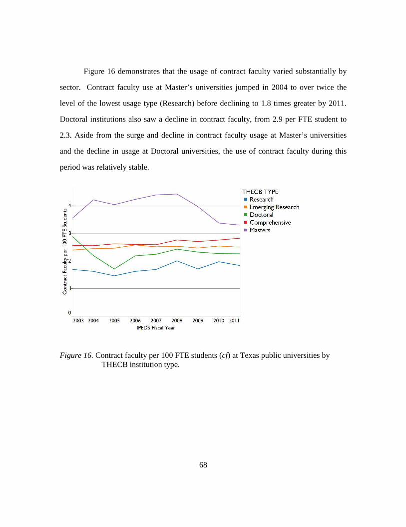
68

Figure 16 demonstrates that the usage of contract faculty varied substantially by

sector. Contract faculty use at Master’s universities jumped in 2004 to over twice the

level of the lowest usage type (Research) before declining to 1.8 times greater by 2011.

Doctoral institutions also saw a decline in contract faculty, from 2.9 per FTE student to

2.3. Aside from the surge and decline in contract faculty usage at Master’s universities

and the decline in usage at Doctoral universities, the use of contract faculty during this

period was relatively stable.

Figure 16. Contract faculty per 100 FTE students (cf) at Texas public universities by THECB institution type.

69

The next faculty measure Martin and Hill define is the ratio of part-time faculty

per 100 FTE students (ptf). Figure 17 presents the statewide average for this variable. As

with the contract faculty indicator, use of part-time faculty peaked in 2008 and was lower

in 2011 than 2003 (-7%).

Figure 17. Part-time faculty per 100 FTE students (ptf) at Texas public universities.

70

Figure 18 presents part-time faculty by THECB institution type. The surge then

decline of contract faculty at Master’s institutions is repeated here among part-time

faculty per FTE student. The overall decline in contract faculty at Doctoral institutions,

however, did not occur among the part-time faculty. In addition, from a low bar,

Research institutions displayed increasing part-time faculty, from 0.4 per FTE student to

0.6.

Figure 18. Part-time faculty per 100 FTE students (ptf) at Texas public universities by THECB institution type.

71

The third faculty variable in the Martin and Hill model is the ratio of FTE faculty

per 100 FTE students (ftef). Figure 19 presents the statewide average for this variable.

After six years where this ratio was largely unchanged, it declined from 3.2 in 2008 to 2.8

in 2011 (-13%).

Figure 19. FTE faculty per 100 FTE students (ftef) at Texas public universities.

72

Figure 20 demonstrates how the ftef ratio varied by THECB institution type. The

two THECB institution types with the lowest FTE faculty per student ratios in 2003

(Research and Emerging Research) both experienced modest increases from 2003 to

2011 (1% and 5% respectively). In contrast, the higher faculty to student ratios at the

other three institution types declined (-22% at Doctoral universities, -8% at

Comprehensive universities, and -10% at Master’s universities).

Figure 20. FTE faculty per 100 FTE students (ftef) at Texas public universities by THECB institution type.

73

The final faculty variable used by by Martin and Hill is the ratio of tenure-track

faculty to non-academic professional employees (ttad), essentially a ratio of the

relationship between the academic and non-academic activities of the institution. Figure

21 presents the statewide average of this measure, which declined rapidly during the

study period (-23%).

Figure 21. Tenure-track faculty per professional non-academic staff (ttad) at Texas public universities.

74

Figure 22 demonstrates that the reduction in the ratio of tenured faculty to non-

academic professional staff was concentrated at the Emerging Research, Doctoral,

Comprehensive, and Master’s institutions—declines of -14%, -16%, -24%, and -33%

respectively. In contrast, Research institutions increased their ratio of tenure-track

faculty to administrators over the time period by 6%.

Figure 22. Tenure-track faculty per professional non-academic staff (ttad) at Texas public universities by THECB institution type.

75

Independent Variables—Staff Measurements.

The next set of variables defined by Martin and Hill categorize non-instructional

staff at the institution. A total of five staffing variables are used in their model. The first

of these variables is FTE non-professional employees per 100 FTE students (ftenpro).

Figure 23 presents the statewide average of this measure. After a slow period of modest

decline from 2003 to 2008 this staffing level dropped -17% from 2008 through 2011.

Figure 23. Non-professional FTE staff per 100 FTE students (ftenpro) at Texas public universities.

76

Figure 24 demonstrates how non-professional staffing ratios varied by THECB

institution type. Four of the five THECB institution types exhibited a pattern consistent

with the state average—slow decline from 2003 through 2008, with significant reductions

after that fiscal year. Research institutions, on the other hand, exhibited a different

pattern. Not only did they display overall staffing ratios of non-professional staff almost

twice as high as the rest of the sector but these ratios were largely maintained through the

study period (dropping only -5% from 2003 through 2011).

Figure 24. Non-professional FTE staff per 100 FTE students (ftenpro) at Texas public universities by THECB institution type.

77

The next variable in the Martin and Hill methodology is FTE executive and

professional employees per 100 FTE students (fteadmin). Figure 25 presents the

statewide average for this variable. From 2003 to a peak in 2009 the ratio of these

employees to FTE students increased 17% before declining to an overall increase of 10%

for the entire study period.

Figure 25. Executive and professional FTE staff per 100 FTE students (fteadmin) at Texas public universities.

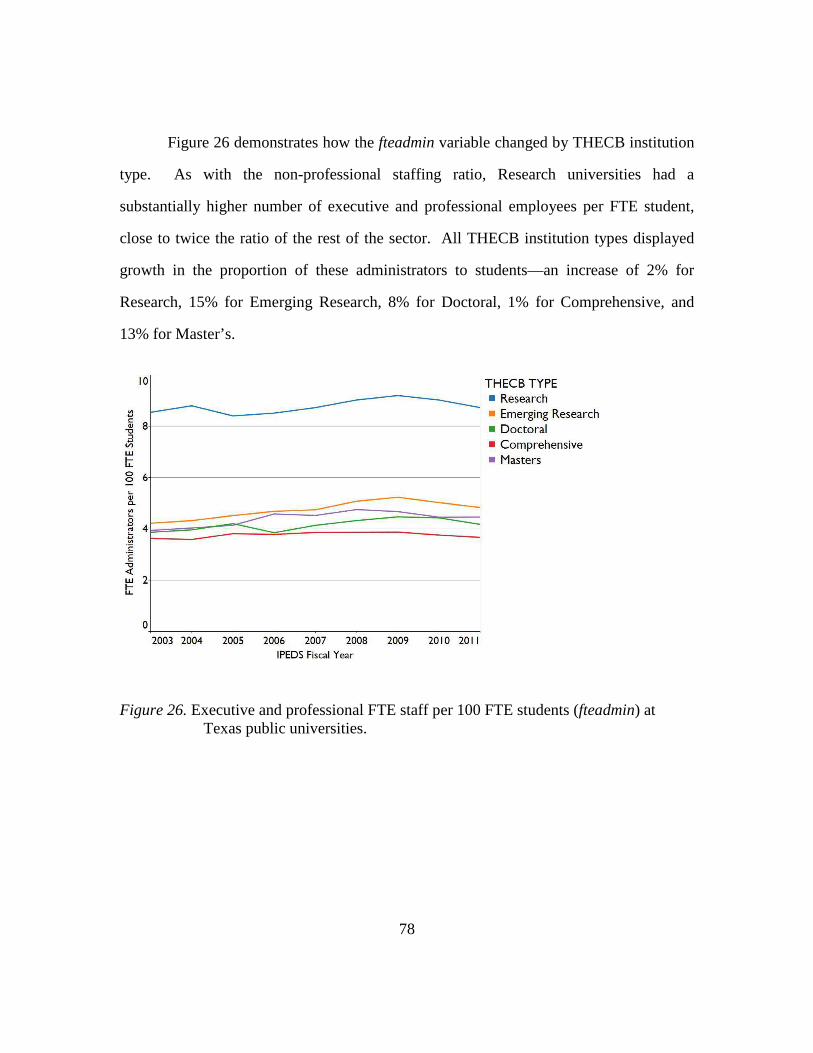
78

Figure 26 demonstrates how the fteadmin variable changed by THECB institution

type. As with the non-professional staffing ratio, Research universities had a

substantially higher number of executive and professional employees per FTE student,

close to twice the ratio of the rest of the sector. All THECB institution types displayed

growth in the proportion of these administrators to students—an increase of 2% for

Research, 15% for Emerging Research, 8% for Doctoral, 1% for Comprehensive, and

13% for Master’s.

Figure 26. Executive and professional FTE staff per 100 FTE students (fteadmin) at Texas public universities.

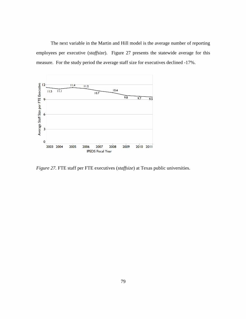
79

The next variable in the Martin and Hill model is the average number of reporting

employees per executive (staffsize). Figure 27 presents the statewide average for this

measure. For the study period the average staff size for executives declined -17%.

Figure 27. FTE staff per FTE executives (staffsize) at Texas public universities.

80

Figure 28 presents the staffsize variable by THECB institution type. Four of the

five THECB institution types displayed declines in the average number of employees per

manager during the study period, with Emerging Research universities demonstrating a

particularly profound reduction from a peak value in fiscal year 2005 to 2011 of -43%.

Research universities staff size dropped -20%, Doctoral universities -10%, and

Comprehensive universities -32%. In contrast to these large reductions, Master’s

universities staff size increased 26% and rose from the second lowest level of staffing

ratio to the highest in the sector.

Figure 28. FTE staff per FTE executives (staffsize) at Texas public universities by THECB institution type.

81

The final two staffing variables show changes in part-time staffing levels. The

first of these variables is the ratio of part-time administrators per 100 FTE students

(ptadmin). Figure 29 presents the statewide average for this variable, which dropped a

total of -37% during this period.

Figure 29. Part-time executive and professional staff per 100 FTE students (ptadmin) at Texas public universities.

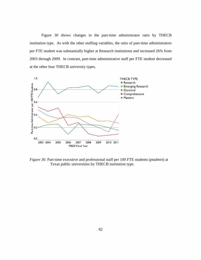
82

Figure 30 shows changes in the part-time administrator ratio by THECB

institution type. As with the other staffing variables, the ratio of part-time administrators

per FTE student was substantially higher at Research institutions and increased 26% from

2003 through 2009. In contrast, part-time administrative staff per FTE student decreased

at the other four THECB university types.

Figure 30. Part-time executive and professional staff per 100 FTE students (ptadmin) at Texas public universities by THECB institution type.

83

The final staffing variable in the Martin and Hill model is the ratio of part-time

non-professional staff per 100 FTE students (ptnpro). Figure 31 presents the statewide

average for this variable, which declined by -47% during the study period.

Figure 31. Part-time non-professional staff per 100 FTE students (ptnpro) at Texas public universities.

84

Figure 32 presents the change in part-time non-professional staff by THECB

institution type. Research class universities are again different than the other THECB

institution types in their large number of part-time non-professional staff per FTE student

as well as their 12% increase in this ratio from 2003 to 2011. In contrast, the ratio of

part-time non-professional staff declined at the other four THECB institution types.

Figure 32. Part-time non-professional staff per 100 FTE students (ptnpro) at Texas public universities by THECB institution type.

85

Independent Variables—Revenue.

The final set of variables used by Martin and Hill measure three sources of

university revenue per FTE student. Figure 33 presents the statewide average for total

revenues per student less investment income (rev). From fiscal year 2003 to fiscal year

2011 rev expanded 9% in real dollars (but declined since 2009).

Figure 33. Total real revenue per FTE student, less investment income (rev) at Texas public universities.

86

Figure 34 presents total revenue per student by THECB institution type. While

this amount increased for all university classes, the already overwhelming lead in real

per-FTE student revenue at Research institutions widened dramatically in both

percentage and absolute terms from 2003 through 2011, from $42,202 to $50,123 (an

increase of 19%). This expansion occurred in the years immediately following tuition

deregulation. Doctoral universities also experienced a major percentage increase in real

revenue from $19,956 to $20,938 (19%). In contrast, Emerging Research universities

raised average revenue per student from $22,587 to $23,230 (3%), Comprehensive

universities from $19,956 to $20,938 (5%), and Master’s universities from $20,937 to

$21,740 (4%).

Figure 34. Total real revenue per FTE student, less investment income (rev) at Texas public universities by THECB institution type.

87

The second revenue variable used by Martin and Hill is “other” operating revenue

(other), a subset of total revenue. Figure 35 shows the statewide average for real other

revenue during the study period. Overall, other income increased 15% during the study

period. While source of revenue is not available in IPEDS, the spike of other income in

fiscal year 2009 correlates with the wide distribution of addition Federal funds from the

economic stimulus provided by the American Recovery and Reinvestment Act.

Figure 35. Real other revenue per FTE student, less investment revenue (other) at Texas public universities.

88

Figure 36 shows how other income changed during the study period by THECB

institution type. The massive revenue advantage for Research universities in total

revenue is also reflected in other revenue. From 2005 until 2011, other revenue at

Research institutions increased from $22,163 to $28,761 (30%), faster than their rate of

total revenue growth. To put that into perspective, Research universities on average

generated more revenue from other sources than other institutions generated from all

sources.

Doctoral universities experienced a dramatic percentage increase in real other

income, from $5,763 to $9,550 (66%). Comprehensive and Master’s universities

displayed smaller gains from $7,348 to $8,134 (11%) and $6,617 and $6,974 (5%)

respectively. Other income at Emerging Research universities actually declined from

$9,258 to $8,525 (-8%).

Figure 36. Real other revenue per FTE student, less interest (other) at Texas public universities by THECB institution type.

89

The final revenue variable used by Martin and Hill is investment income per FTE

student (invest). Figure 37 presents statewide average investment income per student.

(The large negative amount in fiscal year 2009 was due to the recession that began at the

beginning of that fiscal year.) Overall investment income per FTE student decreased in

real terms from $653 to $495 (-24%), however this masks wide fluctuations in yearly

investment income (and demonstrates why removing these funds are important for

understanding strategic behavior on the part of institutions).

Figure 37. Real investment revenue per FTE student (invest) at Texas public universities.

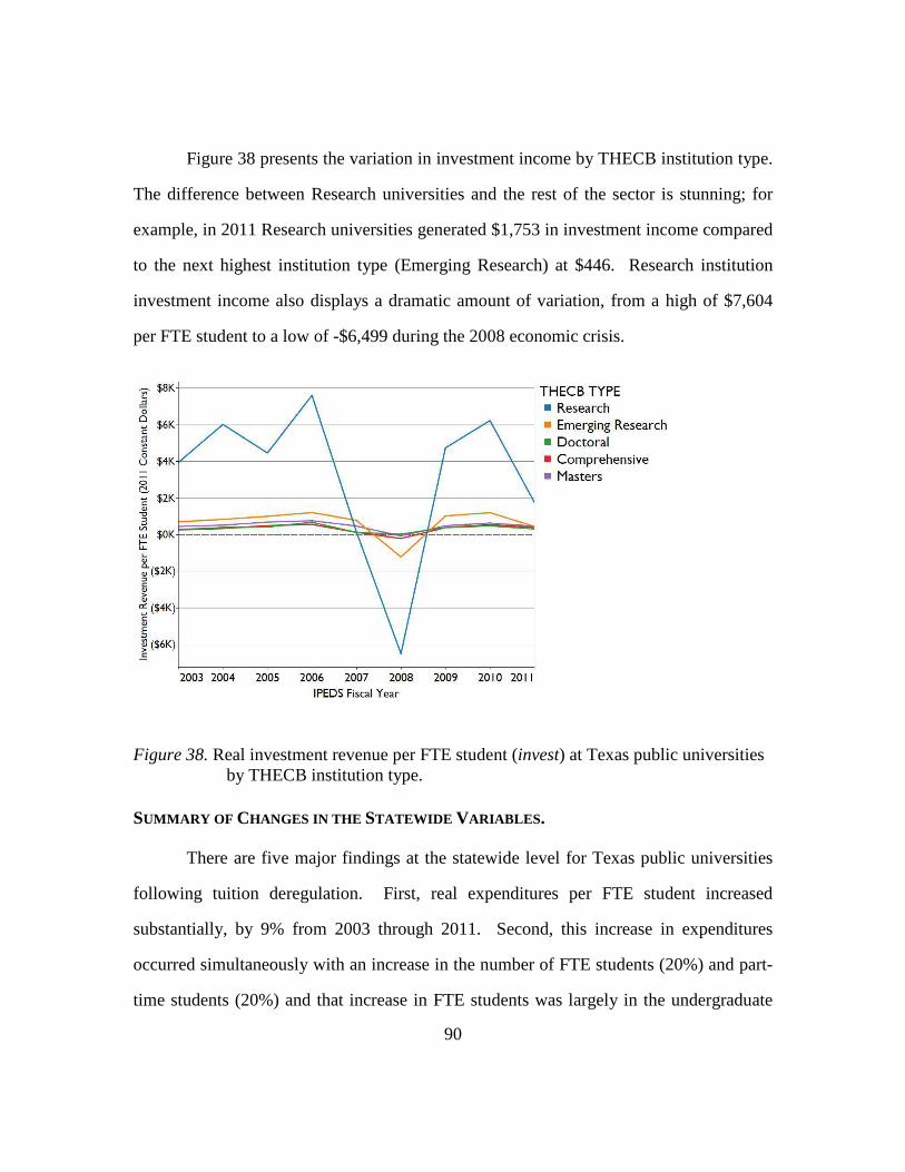
90

Figure 38 presents the variation in investment income by THECB institution type.

The difference between Research universities and the rest of the sector is stunning; for

example, in 2011 Research universities generated $1,753 in investment income compared

to the next highest institution type (Emerging Research) at $446. Research institution

investment income also displays a dramatic amount of variation, from a high of $7,604

per FTE student to a low of -$6,499 during the 2008 economic crisis.

Figure 38. Real investment revenue per FTE student (invest) at Texas public universities by THECB institution type.

SUMMARY OF CHANGES IN THE STATEWIDE VARIABLES .

There are five major findings at the statewide level for Texas public universities

following tuition deregulation. First, real expenditures per FTE student increased

substantially, by 9% from 2003 through 2011. Second, this increase in expenditures

occurred simultaneously with an increase in the number of FTE students (20%) and part-

time students (20%) and that increase in FTE students was largely in the undergraduate

91

category (since graduate students only increased 5%). Third, increases in enrollment and

spending occurred while salaries and benefits were largely flat (0% and 2% respectively).

Fourth, all of these increases were associated with increasing revenue on an FTE student

basis both broadly (9%) and in other revenue (15%). In short, the scope of the public

higher education sector increased dramatically both in real expenditures and enrollment

between fiscal years 2003 and 2011 as tuition deregulation was implemented.

As the scope of the sector increased, substantial changes in staffing patterns

occurred. On the academic side of the university, FTE faculty per FTE students dropped

by -13% while contract faculty and part-time faculty dropped at a smaller rate (-3% and -

7% respectively). On the non-academic side, non-professional positions, both full-time

and part-time, dropped -21% and -47% respectively. In contrast to non-professional

administration and faculty, executive and professional administrators per FTE student

increased by 10%. The drop in non-professional staff and increase in professional staff

led to a -17% decline in average staff size. Finally, the growth in professional

administrators combined with the general decline in faculty per FTE student led to a

decline of -23% in the ratio of tenure-track faculty to non-academic professional staff.

Variations at Research Institutions.

Research institutions displayed substantially lower levels of enrollment growth

than the rest of the sector from 2003 through 2011 (6%). Enrollment growth in graduate

students was similar to the rest of the sector at 4%, so the difference compared to other

THECB institution types occurred due to slow growth in undergraduate enrollment. In

contrast to basically flat enrollment, expenditures per student at these institutions surged.

Already over two times the amount the next highest THECB institution type,

expenditures at Research universities grew faster than any other sector during the study

92

period. These expenditure increases were accompanied by massive revenue growth per

student—19% in total revenues and 30% in other revenues. Consequently, the total

revenue gap between Research universities and the next highest institution type increased

from $19,331 to $26,105 following tuition deregulation.

Staffing pattern changes at Research institutions varied substantially from the rest

of the sector. Full-time faculty per FTE student rose 1% instead of declining. This

institution type displayed the lowest usage of contract faculty and part-time faculty while

its substantially higher proportion of administrators per FTE student at Research

institutions was maintained. Professional and executive staff, two times higher than the

rest of the sector in 2003, increased at a lower rate of 2% through 2011. Non-

professional staff, which dropped precipitously elsewhere, only declined -5% at Research

universities. Part-time non-academic staff, professional and non-professional, both

increased (26% and 12% respectively). Finally, the ratio of tenure-track faculty to

administrators grew 6% (but remained substantially lower than the rest of the sector).

Variations at Emerging Research Institutions.

Enrollment at Emerging Research institutions increased at a greater percentage

than the statewide average (25%) and graduate student enrollment increased substantially

more than the statewide average (27%). The increase in student enrollments was

accompanied by a modest increase in the FTE student/faculty ratio of 5% while the

tenure-track to professional staff ratio declined at a lower rate than the statewide average

(-14%). The only variation in non-academic staffing that deviated from the statewide

average was an extraordinarily sharp decline in the average staff size variable, dropping

-41% during the study period. Another major variation in this sector was a substantially

lower level of average staff salaries and benefits than the other four THECB institution

93

types. Finally, Emerging Research institutions experienced by far the lowest average

increase in total revenue per FTE student of any THECB institution type, only increasing

3% from 2003 through 2011.

Variations at Doctoral Institutions.

Doctoral institutions exhibited the highest average rate of FTE student enrollment

increase in the sector (28%) in addition to a large percentage increase in graduate

enrollment (61%), particularly from 2009 to 2011. While student enrollments increased

across the board, academic staffing levels did not keep pace as the overall FTE student to

faculty ratio declined -22% (the greatest of any THECB institution type). Doctoral

institutions displayed a large decline in contract faculty of -27% and a reduction of the

ratio of tenure-track faculty to administrators of -16%. Their large growth in student

enrollments was accompanied by the second highest rate of total revenue growth of any

THECB institution type (19%).

Variations at Comprehensive Institutions.

FTE student enrollment at Comprehensive institutions grew faster than the

statewide average at 22%. This enrollment increase was accompanied by the second

largest decline in the ratio of tenure track faculty to administration (-24%) and the second

largest reduction in staff size (-32%). Comprehensive institutions experienced the third

highest growth in total revenue per FTE student.

Variations at Master’s Institutions.

Overall student enrollment increases at Master’s institutions followed the state

average, with the exception of a lower than average decline in part-time FTE enrollment

of -11%. These institutions began the study period with contract faculty and part-time

faculty per FTE student ratios over twice the level of the next highest institution type.

94

While this staffing pattern declined during the study period, these ratios remained higher

than other institutional types through 2011. These institutions experienced the highest

reduction in the ratio of tenure track faculty to administration of any THECB institution

type (-33%) and were the only type to see an increase in administrative staff size (26%).

Total revenue increased at a lower rate than the state average (4%). One final, and rather

surprising, difference was that the average salary at these institutions was the highest of

any THECB institution type across the study period.

SUMMARY OF CHANGES IN THE PUBLIC HIGHER EDUCATION SECTOR FROM 2003 TO

2011

Statewide real average expenditures per FTE student increased 9% from fiscal

year 2003 to fiscal year 2011, with Research institutions growing more rapidly than other

institution types (14%) and expanding their already substantial expenditure advantage

compared to other THECB institution types. Salaries and benefits generally remained at

a constant real level, with benefits modestly outpacing salaries. Emerging Research

institutions displayed substantially lower levels of salary per FTE employee while

Master’s and Research institutions displayed higher levels.

As expenditures per FTE student increased, FTE student enrollments increased

with growth concentrated among undergraduates. Increases in enrollment were focused

in the Emerging Research, Doctoral, and Comprehensive universities while Research and

Master’s universities grew more slowly. Graduate student enrollment was flat overall;

however, it increased at Emerging Research and Doctoral universities. Statewide part-

time enrollment generally increased, however this growth did not occur at Research

institutions and was more modest at Master’s institutions.

Across the sector, the ratio of FTE faculty per FTE student dropped during the

study period with contract and part-time faculty per FTE student dropping at lower rates

95

and potentially indicating some switching of tenure-track to non-tenure track positions.

This trend was less pronounced at Emerging Research institutions while the faculty FTE

student ratio at Research institutions increased modestly

As faculty employment per FTE student declined across the sector, executive and

professional administrative staff increased by 10% and non-professional administrative

staff declined -21%. Research institutions, on the other hand, displayed a low level of

growth among FTE faculty and FTE executive and professional staff per FTE student,

however, these ratios remained far above the rest of the sector. The ratio of tenure-track

faculty to FTE administrators declined at all institution types but Research universities

(which experienced a 6% increase).

96

Chapter 5: Econometric Model Results

Chapter 5 details the results of the econometric model described in Chapter 3. It

begins by interpreting the results of the five regression models deployed in this research.

This analysis examines both the statistical significance and influence (as measured by the

parameter estimate) of the independent variables and uses differences between the five

models to identify sources of heteroscedasticity, autocorrelation, and influential outliers.

Following this, the chapter presents figures that show variation from 2003 to 2011 for

each of the instruments in the model by THECB institution type. It next displays figures

demonstrating the total estimated real averages for Baumol and Bowen expenditures by

fiscal year and the ratio of these expenditures. The chapter concludes by answering the

research questions that motivate this research.

PROBLEM STATEMENT AND RESEARCH QUESTIONS

This chapter presents the statistical results from an econometric model measuring

Texas public universities expenditures following tuition deregulation. Were expenditures

largely constrained by macroeconomic factors in the general labor market (the Baumol

hypothesis) or do unresolved agency problems, institutional interests, and other

microeconomic explanations instead explain expenditures (the Bowen hypothesis)? This

study addresses two research questions.





funds?

97

PRESENTATION OF THE REGRESSION MODELS

The first section of this chapter presents the general econometric model I

constructed following the methodology described in Chapter 3. Table 1 compares the

standard errors for the intercept and the control variables used in the study. The

parameter estimate B may be read as the dollars explained by a one-unit change in the

parameter (or in the case of categorical control variables by being part of that category).

The White standard error column (HC) reports adjustments to OLS standard errors to

correct for heteroscedasticity. The Newey West column (HAC) reports adjustments to

correct for heteroscedasticity and autocorrelation. The columns for heteroscedasticity

and autocorrelation report differences between the OLS standard error and the HC and

HAC estimators. Differences from 10% to 24% are classified as “Some,” differences

from 25% to 49% are classified as “Moderate,” and differences of 50% or greater are

classified as “High.”

King and Roberts (2015) argue that applying HC standard error corrections

should not be considered a model fix. Instead, differences in standard errors should be

seen as evidence of model misspecification and that the proper response when confronted

with differences in standard errors due to heteroscedasticity is to investigate whether

modifications to the functional form of the regression equation can minimize or eliminate

the non-constant variance. Differences in standard errors due to autocorrelation, on the

other hand, are generally due to the OLS procedure not properly discounting the amount

of information contained in serially situated observations (Horchle, 2007)—with the

caveat that autocorrelation due to seasonality can be addressed through changes to the

functional form of the regression equation (Box, Jenkins, & Reinsel, 1994).

98

Table 1: OLS, White (HC), and Newey West (HAC) Regression Results—Intercept and Control Variables

Ordinary Least Squares (OLS) White (HC) Newey West (HAC)

Parameter B SE B p

SE B p

SE B p OLS to

HC OLS to HAC Hetero. Auto.

Intercept -8,037.32 1,971.15 <.001 2,140.50 <.001 2,804.00 .005 9% 42% No Moderate Research 8,930.92 1,723.86 <.001 1,758.50 <.001 2,213.90 <.001 2% 28% No Moderate Emerg. Research 1,540.74 731.54 .036 738.90 .038 887.90 .084 1% 21% No Some Doctoral 82.45 373.14 .825 388.80 .832 550.20 .881 4% 47% No Moderate Comprehensive 965.13 338.19 .005 401.30 .017 559.90 .086 19% 66% Some High Year: 2011 998.72 509.95 .051 560.40 .076 553.60 .072 10% 9% Some No Year: 2010 1,631.08 508.78 .002 565.20 .004 587.30 .006 11% 15% Some Some Year: 2009 557.21 525.83 .290 610.20 .362 660.30 .400 16% 26% Some Some Year: 2008 378.89 507.29 .456 615.40 .539 649.90 .560 21% 28% Some Moderate Year: 2007 -124.05 489.28 .800 521.70 .812 568.30 .827 7% 16% No Some Year: 2006 156.38 433.99 .719 523.90 .766 527.00 .767 21% 21% Some Some Year: 2005 -243.24 409.79 .553 417.30 .561 409.70 .553 2% 0% No No Year: 2004 -11.72 392.91 .976 438.60 .979 373.20 .975 12% -5% Some No* Model R2 .95 Notes: Parameter estimates are nominal values. Differences in standard errors between OLS and White/Newey West are classified as Some between 10% and 24%, Moderate between 25% and 50% and High at 50% or above. Reference values for the fixed effect variables are Master’s universities and fiscal year 2003. * HAC standard error is smaller than OLS.

99

Three of the four institution types exhibit significant difference from the reference

Master’s institutions in the OLS model: Research ($8,931, p < .001), Emerging Research

($1,541, p = .036), and Comprehensive ($965, p = .005). Doctoral institutions display

little difference from the reference and their parameter has low significance (p = .825).

The fixed effect variables controlling for institution type exhibit virtually no

increases in standard errors due to heteroscedasticity when the HC estimator is applied,

indicating that THECB institution type is an effective control for underlying differences

in expenditures between the universities. In contrast, the HAC estimator demonstrates

that all institution-type variables exhibit increases in standard errors when autocorrelation

is corrected. Accordingly, the level of significance reported by OLS for these variables

should be discounted in favor that reported by the HAC estimator.

Taking into account the HAC reduced standard errors, Research universities

continue to display a very high level of statistically significant deviation from Master’s

universities (p < .001) while the significance of the Emerging Research and

Comprehensive institution-type fixed effect variables decline to p = .084 and p = .086,

respectively. In other words, the HAC estimator suggests that there is only limited

statistically significant difference between the fixed effect variables for THECB

institutions other than Research universities.

The year fixed effect variables generally exhibit some heteroscedasticity with six

of the eight have a difference in standard errors of 10% or greater. Fiscal years that

occurred following tuition deregulation exhibit smaller standard errors when

autocorrelation is accounted for, while fiscal years following tuition deregulation exhibit

larger standard errors. This is evidence of discontinuity created by the policy change.

Under OLS, only the parameter estimate for fiscal year 2010 displays a high level of

statistical significance (p = .005); fiscal year 2011 displays some statistical significance

100

(p = .051). Adjustments made by the HAC estimator to correct for autocorrelation

degrade these to p = .006 and p = .072, respectively.

Table 2 compares the parameter estimates from the OLS model with the

parameter estimates generated by the Huber (M) and Yohai (MM) estimators. Recall that

the M-estimator adjusts the solution of the regression equation to account for

heteroscedasticity while the MM-estimator adjusts for heteroscedasticity and influential

outliers.8 The parameter estimates from the M-estimator for the THECB institution-type

control variables are similar to OLS results while the MM-estimator parameter estimates

are more influential than those from OLS. This difference suggests that outliers are

contaminating the OLS regression results for the institution type fixed-effect variables in

addition to the autocorrelation identified in Table 1. Because the BLUE quality of OLS

can be easily violated due to the presence of influential outliers, this finding suggests that

parameter estimates generated by the MM-estimator should be used to generate estimated

values for Baumol and Bowen expenditures.

Applying the M-estimator to the yearly fixed effect variables yields both greater

influence in the parameter estimates and improvements in statistical significance (an

expected result given the heteroscedasticity identified by the HC estimator). The

influence of the parameter estimates and their level of statistical significance jumps again

using the MM-estimator, indicating that outliers also skew the parameter estimates for

these variables. The increase in statistical significance for some of the fiscal year fixed

effect variables when moving from OLS to the MM-estimator is substantial: 2011 (p =

.051 to p = .001), 2010 (p = .002 to p < .001), 2009 (p = .290 to p = .002), and 2008 (p =

.456 to p = .004) and supports using the MM-estimator to generate these values.

8 During the generation of these model results, the PROC ROBUSTREG procedure identified a number of influential outliers and recommended the use of the MM-estimator due to these outliers.

101

Table 2: OLS, Huber (M-Estimator), and Yohai (MM-Estimator) Regression Results—Intercept and Control Variables

Ordinary Least Squares (OLS) Huber (M-estimator) Yohai (MM-estimator) Parameter B SE B p B SE B p B SE B p OLS to M OLS to MM Intercept -8,037.32 1,971.15 <.001 -7,241.91 1,528.66 <.001 -6,149.38 1,629.48 <.001 -10% -23% Research 8,930.92 1,723.86 <.001 8,976.52 1,336.88 <.001 8,508.82 1,452.46 <.001 1% -5% Emerg. Research 1,540.74 731.54 .036 1,470.35 567.33 .010 1,072.30 610.25 .079 -5% -30% Doctoral 82.45 373.14 .825 35.60 289.38 .902 -181.39 310.41 .559 -57% * Comprehensive 965.13 338.19 .005 897.31 262.27 .001 561.60 287.47 .051 -7% -42% Year: 2011 998.72 509.95 .051 1,234.79 395.47 .002 1,418.69 423.15 .001 24% 42% Year: 2010 1,631.08 508.78 .002 1,819.25 394.57 <.0001 1,984.65 422.55 <.001 12% 22% Year: 2009 557.21 525.83 .290 1,033.07 407.79 .011 1,329.79 435.66 .002 85% 139% Year: 2008 378.89 507.29 .456 787.39 393.41 .045 1,193.15 419.08 .004 108% 215% Year: 2007 -124.05 489.28 .800 382.92 379.44 .313 613.02 402.46 .128 * * Year: 2006 156.38 433.99 .719 220.26 336.56 .513 368.81 358.22 .303 41% 136% Year: 2005 -243.24 409.79 .553 -92.49 317.80 .771 11.26 333.88 .973 -62% * Year: 2004 -11.72 392.91 .976 51.10 304.71 .867 50.21 327.68 .878 * * Model R2 .95 .86 .73 Notes: Parameter estimates for Year variables are nominal values. Reference values for the fixed effect variables are Master’s universities and fiscal year 2003. * Sign change in parameter estimate.

102

In addition to the formal control variables described above, Martin and Hill’s

methodology includes two instruments that measure shifting expenditures within

institutions based on program scale changes (from changes in the distribution of students)

and institutional cost savings (from changes in the distribution of staff). Table 3 reports

the OLS results and the HC/HAC standard errors for these two instruments.

For the Scale Change instrument, the bulk of the explanatory value in the OLS

model lies in the ratio of graduate assistants per FTE student (ta). The HC estimator

indicates that this variable contains some heteroscedasticity while the HAC estimator

suggests it also displays high levels of autocorrelation. Despite these issues, the level of

significance of the variable remains high in all three models (p < .001 for OLS and p =

.002 for HAC).

The number of full-time graduate students (ftgrad) displays a high level of

statistical significance (p = .029). While the HC estimator does not change this result, the

HAC estimator suggests a moderate amount of autocorrelation resulting in a substantial

drop in statistical significance to p = .110. The ftestu and ptstu variables display low

levels of statistical significance in OLS (p = .737 and p = .193) both of which are

degraded under HAC. Because the sign for ta is positive while the sign for ftgrad is

negative, the OLS results for the Scale Change instrument suggest a trade-off between

expenditures on graduate assistants and revenues from graduate students. A negative

value from this instrument would present evidence that graduate education cross-

subsidizes other functions within universities.

In the Cost Savings instrument, all four variables are highly significant in OLS.

Under the HC and HAC estimators, contract faculty (cf) and part-time faculty (ptf)

exhibit no heteroscedasticity or autocorrelation. Full-time equivalent non-professional

employment (ftenpro) displays some heteroscedasticity and moderate autocorrelation.

103

Part-time non-professional administrative employment (ptnpro) displays moderate levels

of autocorrelation. As a result, the HAC estimator reduces the statistical significance of

these two variables from a high level (p = .004 for ftenpro and p = .013 for ptnpro) to a

moderate level (p = .051 for ftenpro and p = .059 for ptnpro). This result suggests that

the contribution of non-professional staffing ratios to explaining university expenditures

is less than the base OLS model predicts due to serially correlated variation.

The overall results of the Cost Savings instrument suggest that, while higher

ratios of part-time faculty per FTE student do decrease total expenditures as expected,

contract faculty are more expensive than tenure track faculty on a per FTE student basis.

This is a surprising and interesting finding; it is possible that the substitution of contract

faculty for tenure-track faculty results not in short term savings costs but rather in

avoiding long-term financial constraints (and that universities pay a premium for this

flexibility).

Interpretation of the administrative employee parameters is straightforward.

Expenditures increase due to full-time equivalent non-professional employment per FTE

student while part-time employment reduces expenditures.

104

Table 3: OLS, White (HC), and Newey West (HAC) Regression Results— Scale Changes and Cost Savings

Ordinary Least Squares (OLS) White (HC) Newey West (HAC) Instrument Parameter B SE B p

SE B p

SE B p

OLS to HC

OLS to HAC Hetero. Auto.

Scale Changes ftestu -0.015 0.044 .737 0.041 .711 0.049 .757 -9% 9% No No* ftgrad -0.59 0.27 .029 0.29 .044 0.37 .110 8% 36% No Moderate ptstu -0.090 0.069 .193 0.050 .074 0.074 .223 -27% 7% No* No ta 714.23 148.63 <.001 183.20 <.001 232.10 .002 23% 56% Some High Cost Savings cf 950.25 391.36 .016 389.70 .015 385.00 .014 0% -2% No* No ptf -1,043.79 290.83 <.001 315.70 .001 304.60 .001 9% 5% No No ftenpro 398.10 138.27 .004 152.60 .010 202.60 .051 10% 47% Some Moderate ptnpro -208.50 83.31 .013 89.12 .020 110.10 .059 7% 32% No Moderate Model R2 .95 Notes: Parameter estimates are nominal values. Differences in standard errors between OLS and White/Newey West are classified as Some between 10% and 24%, Moderate between 25% and 50% and High at 50% or above. * HC/HAC standard error is smaller than OLS.

105

Table 4 compares the parameter estimates for the Scale Changes and Cost Savings

instrument for the OLS model and robust regression estimators. In the Scale Change

instrument, the graduate assistant variable remains highly statistically significant,

however using the MM-estimator reduces the influence of its parameter estimate from B

= 714.23 to B = 465.26. Application of the MM-estimator also reduces the statistical

significance and influence of expenditures attributable to full-time graduate enrollment (p

= .029 to p = .154 and B = -0.59 to B = -0.32). In contrast, the MM-estimator improves

the statistical significance and influence of part-time student enrollment (p = .193 to p =

.033 and B = -0.090 to B = -0.12). Both results indicate the presence of

heteroscedasticity and influential outliers.

All four variables in the Cost Savings instrument are highly statistically

significant in the OLS model as in well as in the robust regressions. The influence of

full-time equivalent, non-professional staff (ftenpro) decreases from B = 398.10 to B =

258.90 when the MM-estimator is applied. The substantial increase in influence for

contract faculty (cf) (B = 950.25 to B = 1,251.15) and for part-time faculty (ptf) (B = -

1,043.79 to B = -1,284.79) suggests that these variables are subject to both

heteroscedasticity and influential outliers in the OLS model and supports the use of the

MM-estimator to generate estimated expenditure values for these variables.

106

Table 4: OLS, Huber (M-Estimator), and Yohai (MM-Estimator) Regression Results—Scale Changes and Cost Savings

Ordinary Least Squares (OLS) Huber (M-estimator) Yohai (MM-estimator) Parameter B SE B p B SE B p B SE B p OLS to M OLS to MM Scale Changes ftestu -0.015 0.045 .737 -0.035 0.035 .386 -0.025 0.037 .490 100% 67% ftgrad -0.59 0.27 .029 -0.35 0.21 .097 -0.32 0.22 .154 -41% -46% ptstu -0.09 0.069 .193 -0.095 0.054 .077 -0.12 0.055 .033 5% 31% ta 714.23 148.63 <.001 539.04 115.26 <.001 465.26 122.92 <.001 -25% -35% Cost Savings cf 950.25 391.36 .016 1,129.62 303.51 <.001 1,251.15 327.56 <.001 19% 32% ptf -1,043.79 290.83 <.001 -1,174.00 225.54 <.001 -1,284.79 245.19 <.001 12% 23% ftenpro 398.10 138.27 .004 338.35 107.23 .002 258.90 114.93 .024 -15% -35% ptnpro -208.50 83.31 .013 -238.20 64.61 <.001 -209.01 68.09 .002 14% 0% Model R2 .95 .86 .73 Note: Parameter estimates are nominal values.

107

Finally, the Martin and Hill methodology contains four instruments used to

determine the effect of Baumol and Bowen effects. Table 5 shows these instruments.

The Compensation instrument measures the relationship between expenditures and

salaries and benefits. In the base OLS model, both of these variables are highly

significant (p < .001 and p = .001). The parameter estimates suggest that one dollar of

salary is equivalent to 2.8 dollars of benefits in explaining expenditures.

The HC estimator suggests there is some heteroscedasticity in the salary variable

while the HAC estimator suggests that both variables in the Compensation instrument

display substantial autocorrelation (not a surprising result given the low level of

employee attrition at universities and the relationship previous year salary has on the

following year). This autocorrelation degrades the statistical significance of the variables

using the HAC estimator. The staffsal variable remains highly significant (p < .001 to p

= .006) while the significance of the benstaff variable drops from p = .001 to p = .062.

Two of the four variables in the Productivity instrument are highly significant in

the OLS model: full-time administrators per FTE student (fteadmin) (p < .001) and part-

time administrators per FTE student (ptadmin) (p = .007). Both ratios are associated with

increased expenditures. Employing the HC estimator results in higher standard errors for

the full-time administrator variable suggesting some heteroscedasticity exists; however,

since the statistical significance of fteadmin remains unchanged at p < .001 there does not

appear to be a need to include a quadratic term for this variable in the functional form of

the model (as Martin and Hill employ).

108

Table 5: OLS, White (HC), and Newey West (HAC) Regression Results—Baumol and Bowen Instruments

Ordinary Least Squares (OLS) White (HC) Newey West (HAC) Instrument Parameter B SE B p

SE B p

SE B p

OLS to HC

OLS to HAC Hetero. Auto.

Salary and Benefits

staffsal 0.069 0.016 <.001 0.018 <.001 0.025 .006 14% 57% Some High benstaff 0.16 0.047 .001 0.049 .002 0.062 .012 5% 32% No Moderate Productivity ftef -714.78 409.22 .082 397.40 .073 456.20 .118 -3% 11% No * Some fteadmin 1,363.74 205.63 <.001 238.10 <.001 253.00 <.001 16% 23% Some Some ptadmin 758.97 277.54 .007 292.40 .010 297.60 .011 5% 7% No No staffsize -3.42 14.66 .816 17.92 .849 26.820 .899 22% 83% Some High Revenue rev 0.69 0.057 <.001 0.070 <.001 0.092 <.001 -13% 61% No* High other -0.54 0.064 <.001 0.080 <.001 0.097 <.001 -14% 50% No* High invest -0.074 0.079 .351 0.089 .406 0.101 .466 -12% 28% No* Moderate Governance ttad 555.44 535.13 .300 623.70 .374 588.00 .346 17% 10% Some Some Model R2 .95 Notes: Parameter estimates are nominal values. Differences in standard errors between OLS and White/Newey West are classified as Some between 10% and 24%, Moderate between 25% and 50% and High at 50% or above. * HC standard error is smaller than OLS.

109

The full-time equivalent faculty ratio is on the edge of statistical significance in

the OLS model; however, this variable displays some autocorrelation and its statistical

significance is diminished in the HAC estimator (p = .082 to p = .118). Finally, the ratio

of staff size to number of administrators displays very low statistical significance (p =

.816). Because it also demonstrates some heteroscedasticity and a high degree of

autocorrelation (the highest variance in standard errors in this study) the low level of

significance for this variable is further degraded in the HAC estimator (p = .899).

Two variables in the Revenue instrument in the OLS model are highly significant:

total revenue less investment income (rev) and other income (other) (both p < .001).

Investment income (invest) displays a low level of statistical significance (p = .351). As

in Martin and Hill’s results, rev is associated with increases in expenditure while other is

associated with declines. In the model, core revenues function as an omitted variable.

Since the sign of rev is positive, this indicates that an increase in total revenue leads to a

larger increase in expenditures than the same amount of increase in core revenue.

Similarly, an increase in the other revenue variable implies that revenue from these

sources results in lower levels of expenditures than core revenue. These results could be

related to the relative long-term stability of different revenue sources.

None of the three variables in the Revenue instrument display increased standard

errors due to heteroscedasticity; in fact, all display reduced standard errors in the HC

estimator.9 All three variables display moderate to high levels of autocorrelation;

however, this autocorrelation does not degrade the statistical significance of the total

revenue or other income variables (both of which remain at p < .001).

9 It is possible these variables represent an example of a rare form of heteroscedasticity with non-constant, lower variance in the middle of the distribution.

110

The Governance instrument has one variable—the ratio of tenure-track faculty to

administrators. The variable does not display statistical significance in the OLS model

and this lack of significance is degraded further by heteroscedasticity. Performing a

quadratic transformation on this variable (as suggested by Martin and Hill) does not

result in an increase in statistical significance and its quadratic functional form does not

display the global minimum of Martin and Hill’s model. This finding merely indicates

that an increase in the ratio of tenure track faculty to FTE students increases expenditures

with some diminishing returns.

Table 6 presents the robust regression estimators for the instruments measuring

Baumol and Bowen effects. The first of these is the Compensation index. The M-

estimator suggests that some heteroscedasticity exists in the salary variable (confirming

the analysis of standard errors). More significantly, the MM-estimator suggests that the

OLS parameter estimates for this variable are substantially inflated by the presence of

influential outliers and this reduces the influence of the salary variable (B = 0.07 to B =

0.051) and the benefits variable (B = 0.16 to B = 0.12). Since Baumol effects are

captured only by this instrument, this result suggests that the OLS regression solution

overestimates Baumol expenditures due to outliers and provides a strong reason to use

the MM-estimator in generating estimates for Baumol and Bowen values.

111

Table 6: OLS, Huber (M-Estimator), and Yohai (MM-Estimator) Regression Results—Baumol and Bowen Instruments

Ordinary Least Squares (OLS) Huber (M-estimator) Yohai (MM-estimator) Parameter B SE B p B SE B p B SE B p OLS to M OLS to MM Salary and Benefits staffsal 0.069 0.016 <.001 0.058 0.012 <.001 0.051 0.013 <.001 -16% -25% benstaff 0.16 0.047 .001 0.14 0.036 <.001 0.12 0.038 .001 -8% -21% Productivity ftef -714.78 409.22 .082 -885.68 317.36 .005 -1,052.22 337.99 .002 24% 47% fteadmin 1,363.74 205.63 <.001 1,479.64 159.47 <.001 1,531.14 178.13 <.001 8% 12% ptadmin 758.97 277.54 .007 640.19 215.23 .003 496.68 229.18 .030 -16% -35% staffsize -3.42 14.66 .816 -13.73 11.37 .227 -21.65 12.75 .090 301% 532% Revenue rev 0.69 0.057 <.001 0.68 0.044 <.001 0.68 0.050 <.001 -1% -1% other -0.54 0.064 <.001 -0.52 0.050 <.001 -0.49 0.055 <.001 -4% -9% invest -0.074 0.079 .351 0.0082 0.061 .893 0.082 0.070 .239 * * Governance ttad 555.44 535.13 .300 981.03 415.00 .018 1,261.18 468.71 .007 77% 127% Model R2 .95 .86 .73 Notes: Parameter estimates are nominal values. * Sign change in parameter estimate.

112

The robust regression solutions lead to little change in the parameter estimate and

statistical significance of full-time administrators per FTE student; the variable remains

both significant and influential. In contrast, the robust regression estimators degrade the

statistical significance and influence of the part-time administrator variable (p = .007 to p

= .030 and B = 758.97 to B = 498.68) indicating that outliers skew this variable.

In contrast, application of the M-estimator leads to a dramatic increase in

statistical significance (from p = .082 to p = .005) for the full-time faculty per FTE

student variable and this significance is improved further by the MM-estimator (p =

.002). This result raises the possibility that the functional form of ftef is misspecified in

the model. I examined this possibility with OLS with a quadratic transformation. The

resulting functional form is slightly concave upwards but expenditures explained by the

non-linear form increase at a rate only slightly above linear. Given this modest change,

and that implementing the MM-estimator corrects for this non-linear relationship, I opted

to avoid sacrificing a degree of freedom to include this transformation in the final model.

An increase in statistical significance and influence between the OLS result and

MM-estimator result of the staffsize variable suggests another potential misspecification

in the model (p = .816 to p = .090 and B = -3.42 to B = -21.65). As with the ftef variable,

I investigated this relationship with a quadratic transformation and it too displayed a

functional form with slightly concave upwards curve. In the case of staffsize, however, in

addition to the slight difference between the linear and non-linear versions of the

independent variable the overall influence of the variable was small (explaining only $72

in expenditures per FTE student at the median value for staffsize). Because the MM-

estimator adjusts this variable well, and because the influence of the variable is so small,

I opted to preserve a degree of freedom and leave the linear term in the model (although a

case could be made for dropping it entirely).

113

Application of the robust regression estimators to the variables in the Revenue

instrument does not change the significance of rev and other variables in the instrument.

There is some indication of modest skew from influential outliers in the other variable

that reduce its influence (B = -0.54 to B = -0.49).

The final instrument in the Martin and Hill framework is Governance, represented

by the ratio of tenure-track faculty to administrators (ttad). Martin and Hill find that this

variable is highly significant in a quadratic transformation, a transformation that results in

a global minimum they interpret as a “Golden Mean” for faculty to staff ratios. As with

the staffsize and ftef variables, the low level of statistical significance (p = .300) in the

OLS model is improved by the M-estimator (p = .018) and MM-estimator (p = .007)

indicating either model misspecification or influential outliers. Accordingly, I also

examined a quadratic transformation of the ttad variable in OLS. Unlike the ftef and

staffsize variables, this transformation did not result in a statistically significant pair of

variables and, unlike Martin and Hill, the functional form did not display a global

minimum. The implication is that the robust regression estimators are performing as they

are designed to—reducing heteroscedasticity and limiting the impact of influential

outliers. A change in functional form to the variable is thus unnecessary.

ESTIMATION OF INSTRUMENT EFFECTS

This presentation of the general model establishes that the data generally display

fairly low levels of heteroscedasticity and some degree of autocorrelation (expected in a

balanced panel dataset). The results of the MM-estimator, however, establish that the

data exhibit substantial contamination from outliers that have measurable impacts on the

standard errors and influence of some of the independent variables in the model. Most

critically, the outliers cause the OLS model to overstate the explanatory value of the

114

Compensation instrument and thus the estimate of Baumol expenditures.10 Accordingly,

this study uses the parameter estimates generated by the MM-estimator to calculate mean

values of the instruments for the five THECB institution types. Since the regression

equations presented above were generated using nominal values, the calculation of yearly

average values also includes a transformation into 2011 constant dollars using a CPI

deflator that corresponds with the Texas fiscal year.

The fixed effect variable controlling for fiscal year presents an opportunity to

examine the overall trend of expenditures following tuition deregulation. Figure 39

shows these values and the difference pre- and post tuition deregulation is dramatic.

Tuition deregulation appears to have led to an increase in per FTE student expenditures

on the order of $1,400 at all universities from pre-deregulation expenditure levels

(averaging $1,512 between fiscal years 2008 but with a spike in 2010).

10 This insight also demonstrates the importance of interrogating a dataset with a variety of different regression techniques.

115

Figure 39. Estimated real expenditure change per FTE student by fiscal year, controlling for other variables.

Figure 40 presents the proportion of expenditures explained by the Scale Change

instrument by THECB institution type. All estimated values of the instrument are

negative. Since the variables with negative parameter estimates were not statistically

significant in the MM-estimator this result suggests potential multicollinearity between

the variables in the instrument. A potential interpretation of the results from this

instrument is that graduate students without support cross-subsidize other functions of the

university beyond expenditures required to support teaching and graduate assistants.

The Scale Change instrument displays substantial variation by research intensity

across the sector, with Emerging Research and Research universities displaying a large

amount of potential cross-subsidy from graduate education to elsewhere in the university.

116

Intriguingly, the amount of the subsidy drops rapidly during the study period at Research

universities, from -$6,943 to -$4,850 (-30%). Given that these universities did not see a

drop in graduate students, this drop must be explained through an expansion in support

for graduate studies through increasing expenditures on teaching and graduate assistants.

Figure 40. Estimated real expenditure changes per FTE Student due to Scale Changes by THECB institution type.

Figure 41 presents estimated values for the Cost Savings control instrument by

THECB institution type. While Martin and Hill report the instrument as measuring a cost

subsidy, the results from this study suggest that the variables in the instrument are related

to higher levels of expenditures. This result occurs because the ratio of contract faculty

to FTE students is associated with higher expenditures than the ratio of tenure-track

faculty to FTE students. A potential explanation for this result is that Texas public

117

universities have been paying a premium for shorter term labor arrangements in lieu of

long-term tenure commitments on a per FTE faculty basis.

From 2003 to 2011, universities shifted dollars between faculty types and this led

to a reduced amount of expenditures the instrument explains (and reflects funds shifted to

other expenditures elsewhere in the institution). The expenditure drop was particularly

pronounced at Research universities ($4,821 to $2,636, -45%) and Doctoral universities

($5,154 to $2,383, -54%). Smaller drops occurred at Emerging Research (-25%),

Comprehensive (-37%), and Master’s universities (-25%).

Figure 41. Estimated real expenditure changes per FTE student due to Cost Savings by THECB institution type.

Compensation accounts for both Baumol and Bowen effects in the Martin and

Hill model (because data limitations do not allow these measures to be broken down by

functional administrative area). Martin and Hill use a statistical correlation between

118

compensation and staffing variables to estimate that 51% of benefit costs and 52% of

salaries are due to Baumol effects. Departing from this approach, I created an OLS

regression model to determine the proportion of salaries and benefits that could be

explained by staffing patterns. This model finds a weaker Bowen relationship to benefits

and salaries than that reported by Martin and Hill: 30% for benefits and 39% for salaries.

In the Martin and Hill methodology, salaries and benefits not explained by Bowen effects

are presumed to be due to Baumol effects, so the remainder of the predicted values of

benstaff and staffsal are distributed to Baumol effects (70% and 61%).

Figure 42 presents the amount of expenditures explained by the Compensation

instrument. There is little variation in overall expenditures by THECB institution type,

with the exception of a lower proportion of explained expenditures at Emerging Research

universities. From 2003 to 2011, all institutions exhibited real drops in expenditures

explained by the Compensation instrument. These drops were of similar scale, ranging

from 13% at Research universities to 19% at Emerging Research universities. This result

suggests that Baumol expenditures diminished during the period of this study (although

there is no clear discontinuity to support a difference before and after tuition

deregulation). The results also suggest that there is little differentiation in

macroeconomic effects across university types.

119

Figure 42. Estimated expenditure changes per FTE student due to Compensation by THECB institution type.

The final three instruments measure various proposed Bowen effects. Figure 43

presents the Revenue instrument, the most important of the three. Unsurprisingly,

Research universities display much higher absolute estimated levels of expenditures

explained by total revenue. During the study period, the proportion of expenditures

explained by this instrument declined for all institution types, ranging from a drop of -7%

at Research universities to -14% at Comprehensive universities. This drop reflects the

rise in other revenue than total revenue (shown in Figure 35 and Figure 36).

120

Figure 43. Estimated real expenditure changes per FTE student due to Revenue by THECB institution type.

The large expenditure difference between Research institutions and the rest of the

sector is also apparent in the proportion of expenditures explained by the Productivity

instrument, displayed in Figure 44. There is also an intriguing discontinuity for these

universities following tuition deregulation, with a sharp decline from $15,848 to $11,107

(-30%) in expenditures. Over the study period Emerging Research universities declined

-17%, Doctoral universities declined -6%, and Comprehensive and Master’s universities

declined -2%. The decline in dollars explained by this instrument is correlated with

research intensity as measured by THECB institution type. The role of full-time

administrators per FTE student in explaining expenditures declined following tuition

deregulation, particularly at Research universities. Thus, the popular view of the role of

“administrative bloat” in increased expenditures when revenues increase is not apparent

in this study.

121

Figure 44: Estimated real expenditure changes per FTE student due to Productivity by THECB institution type.

The Governance instrument is presented in Figure 45. All university types

displayed reductions in the proportion of expenditures explained by the ratio of tenure-

track faculty to administrators. At the beginning of the study period there was a wide

spread of dollars explained by this instrument, in reverse order of research intensity. All

university types displayed declines in the dollars explained by this instrument over the

study period, ranging from -28% at Research universities to -55% at Master’s universities

and these declines appear to be leading to convergence across the entire sector. The

relatively low level of expenditures explained by this instrument, combined with the lack

of support for a quadratic function with a global minimum, means this research does not

support Martin and Hill’s contention that there is a “Golden Mean” balancing the tenure-

track faculty and professional administration and that ameliorates potential agency abuse

from both parties.

122

Figure 45: Estimated real expenditure changes per FTE student due to Governance by THECB institution type.

ESTIMATING TOTAL BAUMOL AND BOWEN EFFECTS

Figure 46 presents total real estimated Bowen expenditures during the study

period. Dollars explained by Bowen expenditures declined for all university types during

the study period. These declines ranged from -14% at Emerging Research universities to

-18% at Research universities. Figure 47 presents total estimated Baumol effects for the

study period. Baumol expenditures also declined across the sector from -13% at

Research universities to -19% at Emerging Research universities.

These drops were balanced by an increase in explained dollars by the fiscal year

fixed effect term and the reduction in negative explained dollars in the Scale Change

instrument. This establishes that, during the period when tuition was deregulated at

Texas public universites, increases in revenue were used to diminish existing subsidies

from graduate education to the rest of the instituition rather than increase either Baumol

or Bowen expenditures.

123

Figure 46: Estimated real expenditure changes per FTE student due to Bowen effects.

Figure 47: Estimated real expenditure changes per FTE student due to Baumol effects.

124

Figure 48 presents the Bowen/Baumol ratio and demonstrates the substantial

difference of these expenditures by THECB institution type, a difference that persists

across the study period. THECB institution types with a stronger research focus display

higher levels of Bowen expenditures relative to Baumol expenditures than other THECB

institution types. These ratios range from a high of 8.4 at Research universities to a low

of 3.7 at Master’s universities. Bowen expenditures relative to Baumol expenditures

increased at Emerging Research (6%) and Doctoral institutions (4%) and decreased at

Research (-5%), Master’s, (-3%), and Comprehensive (-1%) institutions. These results

suggest that institutions aspiring to greater research intensity devote proportionally more

resources to Bowen expenditures during periods of increasing expenditures while those

with fixed missions (either high or low research intensity) see a relative increase in the

proportion of Baumol expenditures.

Figure 48. Bowen-to-Baumol ratio.

125

INVESTIGATING MULTICOLLINEARITY

Given the functional form of the model—multiple indicators combined into single

instruments—I wanted to examine the sources of multicollinearity this specification has

the potential to create. While multicollinearity does not invalidate a regression model,

examining its role can aid in its interpretation, particularly values of parameter estimates.

The analysis of the model presented above suggests two potential sources of

multicollinearity: the relationship of full-time graduate students to graduate assistants and

the relationship of contract faculty to part-time faculty.

My first test procedure was to calculate Variance Inflation Factors (VIF) in the

model (after removing the nominal control variables from consideration) using the PROC

REG function in SAS. Eight variables demonstrated a VIF over 10 (the threshold for

indicating multicollinearity): cf, ptf, ta, ftestu, ftgrad, fteadmin, rev, and other. The cf and

ptf variables are elements of the Cost Savings instrument and the ftestu, ftgrad, and ta

variables are elements of the Scale Change instrument. The other three variables with

potential multicollinearity are parts of the Revenue instrument (rev and other) and the

Productivity instrument (fteadmin). The sources of potential multicollinearity identified

in the presentation of the general model are contained in the first two instruments.

I next conducted a clustering analysis on the interval-ratio variables in the model

to investigate any underlying factors that might link these variables using PROC

VARCLUS. This analysis indicates the presence of seven underlying factors in the data

matrix. Of particular interest is a cluster containing ftestu, ta, and ftgrad, a cluster

containing cf and ptf, and a cluster containing rev and other. This result indicates that the

multicollinearity in seven of the eight variables is explained due to interactions between

with three clusters and that these interactions are contained in single instruments in the

regression model. Finally, the eighth variable (fteadmin) is in a cluster with ttad (the

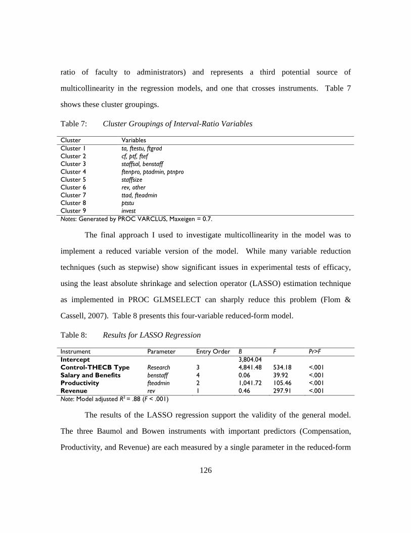
126

ratio of faculty to administrators) and represents a third potential source of

multicollinearity in the regression models, and one that crosses instruments. Table 7

shows these cluster groupings.

Table 7: Cluster Groupings of Interval-Ratio Variables

Cluster Variables Cluster 1 ta, ftestu, ftgrad Cluster 2 cf, ptf, ftef Cluster 3 staffsal, benstaff Cluster 4 ftenpro, ptadmin, ptnpro Cluster 5 staffsize Cluster 6 rev, other Cluster 7 ttad, fteadmin Cluster 8 ptstu Cluster 9 invest Notes: Generated by PROC VARCLUS, Maxeigen = 0.7.

The final approach I used to investigate multicollinearity in the model was to

implement a reduced variable version of the model. While many variable reduction

techniques (such as stepwise) show significant issues in experimental tests of efficacy,

using the least absolute shrinkage and selection operator (LASSO) estimation technique

as implemented in PROC GLMSELECT can sharply reduce this problem (Flom &

Cassell, 2007). Table 8 presents this four-variable reduced-form model.

Table 8: Results for LASSO Regression

Instrument Parameter Entry Order B F Pr>F Intercept 3,804.04 Control-THECB Type Research 3 4,841.48 534.18 <.001 Salary and Benefits benstaff 4 0.06 39.92 <.001 Productivity fteadmin 2 1,041.72 105.46 <.001 Revenue rev 1 0.46 297.91 <.001 Note: Model adjusted R2 = .88 (F < .001)

The results of the LASSO regression support the validity of the general model.

The three Baumol and Bowen instruments with important predictors (Compensation,

Productivity, and Revenue) are each measured by a single parameter in the reduced-form

127

model. The inclusion of only Research as a control for THECB institution type is not a

surprise given the analysis of the Class parameter estimates earlier. Neither the controls

for fiscal years nor the instruments measuring Scale Changes or Cost Savings are

included. The Governance instrument is unrepresented; not an unexpected result given

the low influence of this instrument and the multicollinearity ttad exhibits with fteadmin.

To examine the effect of these three identified sources of possible

multicollinearity I created a cross product terms for the three relationships and

investigated them using OLS. The first of these equations uses ttad and fteadmin. All

three elements (ttad, fteadmin, and ttad*fteadmin) were statistically significant. I

examined the functional form of the cross-product equation generated by the OLS output

in a range of values between the 25th and 75th percentiles of the variables. The resulting

curve displays a slightly concave upwards form and trends upwards but deviation from a

linear relationship is minimal and there is no global maximum or minimum. This

suggests that use of the interaction term is unnecessary. Given that this multicollinearity

crosses two instruments, future research should consider dropping one of these variables.

I next examined the cross product equation for cf, ptf, and cf*ptf. As with the

investigation of ttad and fteadmin, all three terms are statistically significant. The

function exhibits a slightly concave-upwards form with a downward slope and there is no

global maximum or minimum. The curvilinear relationship departs only minimally from

a linear relationship and changing the functional form of the model for this small

adjustment is unnecessary.

The final potential candidate for multicollinearity is the relationship between

ftgrad, ta, and ftgrad*ta. As with the relationship between ttad and fteadmin, the

resulting curve displays a slightly concave upwards form and trends upwards. Deviation

from a linear relationship is minimal and there is no global maximum or minimum.

128

Accordingly, changing the functional form of the regression model to address this mild

multicollinearity is unnecessary.

ANSWERING THE RESEARCH QUESTIONS



The model developed for this research establishes (at least for public universities

in Texas) that the Bowen hypothesis explains substantially more expenditures at

universities than the Baumol hypothesis. The ratio of Bowen to Baumol expenses is

highest at elite Research universities (as high as 8.4) and it is lowest at the least selective,

least research intensive Master’s universities (as low as 3.7). Patterns in expenditure

changes differ depending on the research intensity of the institution.



funds?

Additional tuition did not lead to an expansion of Bowen expenditures relative to

Baumol expenditures at Research institutions; indeed this ratio of Bowen to Baumol

expenditures drops by -5%. This ratio also decreases at Comprehensive and Master’s

universities with low research intensity missions (-1% and -3%). The THECB institution

types of Emerging Research and Doctoral institutions, however, display substantial

increases in Bowen expenditures relative to Baumol expenditures (6% and 4%). This

suggests that the lower-level research universities with aspirations to higher research

intensity shift to an increasing proportion of Bowen expenditures in conditions of

expanding revenue.

129

CONCLUSION

The results presented in this chapter demonstrate that the Martin and Hill

methodology can be used to construct estimates of Baumol and Bowen expenditures for

the entire range of Texas public universities. The model itself possesses a high level of

statistical significance as well as substantial explanatory influence. These results broadly

confirm Martin and Hill’s initial work that Bowen expenditures are a larger proportion of

total university expenditures than Baumol expenses. The findings also confirm my

intuition that launched this project—that research intensity would lead to differential

ratios of Baumol and Bowen expenditures. Unexpectedly, however, it is aspiring

research universities, not top-tier institutions, that display proportional increases in their

ratio of Bowen expenditures to Baumol expenditures. Finally, institutions (particularly

Research universities) appear to have used additional funds from tuition deregulation to

reduce existing subsidies from graduate education to the rest of the institution.

130

Chapter 6: Summary and Conclusions

Chapter 6 of this study reiterates the problem statement this research addresses

and then answers the two research questions it asks. Following this, it reviews the results

for each of the instruments in the econometric model to examine how those results might

inform existing theory on higher education finance. It moves to an assessment of the

significance of the findings from this research, reflections on surprising results and

potential importance for practice, then addresses the limitations of the research. Finally,

the chapter concludes with three concrete proposals for additional research based on the

model developed for this study.

PROBLEM STATEMENT , RESEARCH QUESTIONS, AND METHODS

This chapter summarizes the conclusions of an econometric model that examines

Texas public university expenditures following tuition deregulation. This model

measures expenditures explained by macroeconomic factors in the general labor market

(the Baumol hypothesis) and compares them to expenditures explained by unresolved

agency problems, the pursuit of institutional interests, and other microeconomic factors

(the Bowen hypothesis). This model answers two research questions:





funds?

To answer these questions, the model links expenditures at higher education

institutions with instruments that measure the relative effects of the competing Baumol

and Bowen hypotheses. Institutional mission can have a profound effect on spending

131

decisions, and as a result the model controls for institutional type (and this control allows

the model to answer the second of the research questions). In addition, because the

analysis uses time series data, the model controls for yearly changes in the policy

environment.

Regression equations solved using Ordinary Least Squares (OLS) can be shown

under the Gauss-Markov Theorem to be BLUE—Best Linear Unbiased Estimator (where

“best” means lowest variance of the estimate). Unfortunately, the assumptions required

for OLS estimates to be BLUE are rigorous and under real-world conditions are rarely

met, particularly for panel data such as that used in this research. Deviations from the

Gauss-Markov assumption of constant variance can be partly addressed through changes

to the residual structure that modify the standard errors reported by the procedure without

changing the mean value parameter estimates that OLS provides. These adjusted

standard errors are measured using either heteroscedasticity consistent (HC) or

heteroscedasticity and autocorrelation consistent (HAC) estimators.

Robust regression techniques vary from OLS and OLS-derived approaches such

as HC and HAC because they change the transformation used to solve the regression

equation from a sum of squared values to a different function that modifies the weights

given to residuals when solving the regression equation. This change results in different

standard errors as well as different parameter estimates. The class of robust regressions

designed to address heteroscedasticity are called “M-estimators.” While M-estimators do

an excellent job at controlling for heteroscedasticity, they are ineffective in controlling

for data structures contaminated by influential outliers because they cannot distinguish

between “good” leverage points with information from “bad” leverage points that

represent contaminated data. A separate category of residual transformations attempts to

132

distinguish these two cases, known as “MM-estimators.” In this study, I report five

regression results: OLS, White (HC), Newey West (HAC), Huber (M), and Yohai (MM).

The dataset used in this study generally displays fairly low levels of

heteroscedasticity and some degree of autocorrelation. The results of the MM-estimator,

however, show that the data exhibit substantial contamination of influential outliers that

have measurable impacts on the interpretation and power of the model, most critically in

overstating the explanatory value of the Compensation instrument and thus the

importance of Baumol expenditures relative to Bowen expenditures. As a result, MM-

estimator parameter estimates are used to generate all average values.

RESULTS

Statewide real average expenditures per FTE student at Texas public universities

increased 9% from fiscal year 2003 to fiscal year 2011. Expenditure growth at Research

institutions outpaced other THECB institution types (14%) and expanded their already

substantial spending advantage. Fiscal years following tuition deregulation exhibit

smaller standard errors when autocorrelation is accounted for, while fiscal years

following tuition deregulation exhibit larger standard errors; this is evidence of a

discontinuity created by the policy change. Analysis of yearly fixed effects before and

after tuition deregulation suggests that the policy change led to an increase in

expenditures above pre-deregulation levels on the order of $1,400 in 2011 constant

dollars per FTE student at all universities (Figure 39). As expenditures per FTE student

increased, FTE student enrollments also increased (by 20%). This growth was

concentrated in the undergraduate population.

Constant dollar expenditures explained by Bowen expenditures declined for all

university types during the study period. These declines ranged from -14% at Emerging

133

Research universities to -18% at Research universities (Figure 46). Baumol expenditures

also declined across the sector, from -13% at Research universities to -19% at Emerging

Research universities (Figure 47). These drops in Bowen and Baumol expenditures were

balanced by the across-the-board increases in explained expenditures from the fiscal year

fixed effect term. In addition, institutions (particularly Research universities) appear to

have used additional funds from tuition deregulation to reduce pre-deregulation subsidies

from graduate education to the rest of their institutions. Finding this significant

reallocation of funds provides support for Bowen’s hypothesis. These are savings that

could have been passed to students or returned to the state rather than distributed within

the university. Instead, additional revenue was used to increase the prestige of

universities engaging in research by improving the quality of graduate students by

increasing the subsidy granted these students through graduate and teaching

assistantships.



The model developed for this research establishes (at least for public universities

in Texas) that the Bowen hypothesis explains substantially more expenditures at

universities than the Baumol hypothesis. The ratio of Bowen to Baumol expenses is

highest at elite Research universities (as high as 8.4) and it is lowest at the least selective,

least research intensive Master’s universities (as low as 3.7). Patterns in expenditure

change differ depending on the research intensity of the institution.



funds?

134

Additional tuition did not lead to an expansion of Bowen expenditures relative to

Baumol expenditures at Research institutions; indeed the ratio of Bowen to Baumol

expenditures drops by -5%. This ratio also decreases at Comprehensive and Master’s

universities with low research intensity missions (-1% and -3%). The THECB institution

types of Emerging Research and Doctoral institutions, however, display substantial

increases in the proportion of Bowen expenditures relative to Baumol expenditures (6%

and 4%). This suggests that the lower-level research universities with aspirations to

higher research intensity shift an increasing proportion of spending toward Bowen

expenditures in conditions of expanding revenue.

RELATIONSHIP TO L ITERATURE

As I wrote in the beginning of this study, given that the Baumol and Bowen

hypotheses both have strong theoretical bases, this research was never intended to

“prove” one or the other correct. Rather, my goal was to understand more fully the

relative importance of the two hypotheses. I find that the Bowen hypothesis explains

substantially more expenditure behavior than the Baumol hypothesis for Texas public

universities. In other words, these expenditures are driven more by firm-level

microeconomic explanations than economy-level macroeconomic explanations. Within

the general calculation of Baumol and Bowen costs, the results from six discrete

instruments provide insight into why this relationship exists.

Scale Changes.

The cost function of universities varies based on their mix of graduate and

undergraduate students. One question concerning this relationship is whether a

population of graduate students provides institutions the ability to cross-subsidize

between groups of students or whether graduate education is itself a cost-driver. The

135

results of this study demonstrate that cross-subsidization occurs. The Scale Change

instrument displays substantial variation by research intensity across the sector, with

Emerging Research and Research universities displaying a large amount of potential

cross-subsidy from graduate education to elsewhere in the university.

The estimated amount of this subsidy drops rapidly during the study period at

Research universities, from -$6,943 to -$4,850 (-30%) and -$3,194 to -$2,746 (-14%) at

Emerging Research universities. This drop results from increasing expenditures on

teaching and graduate assistants (Figure 40). Reducing the subsidy from graduate

education to the rest of the university is likely an effort to improve the prestige of these

universities by improving their input of graduate student quality and thus research and

other forms of scholarly output from future students.

Cost Savings.

The results of the Cost Savings instrument suggest that, while higher ratios of

part-time faculty per FTE student do decrease total expenditures as expected, contract

faculty are more expensive than tenure track faculty on a per FTE student basis. This is a

surprising and interesting finding; it is possible that the substitution of contract faculty for

tenure-track faculty results not in short term savings costs but rather in avoiding long-

term financial constraints (and that universities pay a contract faculty a premium for this

flexibility).

From 2003 to 2011, universities reduced expenditures as measured by the Cost

Savings instrument (Figure 41). This expenditure drop was particularly pronounced at

Research universities ($4,821 to $2,636, -45%) and Doctoral universities ($5,154 to

$2,383, -54%). Smaller drops occurred at Emerging Research (-25%), Comprehensive

136

(-37%), and Master’s universities (-25%). These drops are the result of sharp reductions

in the ratio of full-time, non-professional employees (Figure 23).

Revenue.

The proportion of expenditures explained by this instrument declined for all

institution types, ranging from a drop of -7% at Research universities to -14% at

Comprehensive universities. This decline reflects the greater rise in other revenue than

total revenue (Figure 35 and Figure 36) and potentially indicates that these new “other”

revenue sources are less stable than core revenue.

Productivity.

Expenditures explained by the productivity instrument declined following tuition

deregulation, particularly at Research universities (-30%) while Emerging Research

universities declined -17%, Doctoral universities declined -6%, and Comprehensive and

Master’s universities declined -2%. These drops are correlated exactly with research

intensity as measured by THECB institution type (Figure 44) and suggest that the role of

full-time administrators per FTE student in explaining spending declined following

tuition deregulation. This finding indicates that “administrative bloat” following tuition

deregulation is not a driver of increased expenditures. Of particular note is that Research

universities increased their ratio of tenure-track faculty to administrators following tuition

deregulation by 6% (Figure 21).

Compensation.

From 2003 to 2011, all institutions exhibited real drops in expenditures explained

by the Compensation instrument. These drops were of similar scale, ranging from -13%

at Research universities to -19% at Emerging Research universities (Figure 42). Martin

and Hill’s research suggests that 51% of salaries and 52% of benefits can be associated

137

with the Baumol hypothesis. This study demonstrates that, at least for Texas public

universities in this time period, the proportion of Compensation expenditures the Baumol

hypothesis explains is substantially higher than Martin and Hill’s estimate—61% of

salaries and 70% of benefits. Declines in the proportion of expenditures explained by

this instrument directly contradict the Baumol hypothesis that labor costs will increase

faster than the general price level. This finding is corroborated by the variables that

measure salaries and benefits. Figure 11 and Figure 13 demonstrate that salaries rose at

the same level as CPI between 2003 and 2011 while benefits increased by only 2% in real

terms. Compensation also varies little by THECB institution type, suggesting that all

these universities exist in a similar labor market and pay roughly the same market-

clearing wages (with some divergence between lower compensation at Emerging

Research universities and the rest of the sector).

Governance.

The low and declining level of expenditures explained by this instrument,

combined with the failure to find evidence of a quadratic function with a global minimum

for the tenure-track to administrator independent variable, means this study does not

support Martin and Hill’s contention that there is a “Golden Mean” balancing the tenure-

track faculty and professional administration (Figure 45). This removes the single

theoretical internal structure they propose with the potential to restrain expenditure

growth and ameliorate potential agency abuse from both parties.

SIGNIFICANCE

The implications of this research are both important and positive. Imagine, for

example, if the Baumol hypothesis explained a greater proportion of university

expenditures than the Bowen hypothesis. Universities have limited ability to shape and

138

control the broad labor market factors that the Baumol hypothesis invokes to explain

expenditure patterns. Under this hypothesis, the very nature of the labor-intensive

production function at universities would render the expense of providing a university

education beyond the ability of families and society to afford. The consequences of this

increased expense would be an inevitable, revolutionary change in the provision of post-

secondary education. Students of modest means, even solidly middle-class students,

would find themselves locked out of a “traditional” higher education experience. That

experience, in turn would become both a luxury good and a class marker to an even

greater extent than it is currently. Students unable to afford this luxury good would be

forced to settle for second-best options such as impersonal, massive online courses,

experiential credit, and a generally less personalized higher education experience. This

bifurcation of post-secondary education would have profound societal consequences.

Finding that the Bowen hypothesis possesses substantially more explanatory

power than the Baumol hypothesis provides at some hope that incremental changes in

existing structures can address increases in student expenditures. The problem is that

universities lack structures to force choices between these competing good ideas and so

enforce market discipline. In a way, this research provides a case study of what happens

when an effective structure imposing this discipline—Texas’ statutory restrictions on

tuition increases—is removed. One concrete way to address increasing expenditures per

FTE student in Texas, for example, would be to reverse tuition deregulation and once

again require public universities to make the case to the elected leadership of the state for

tuition increases.

Renewing this supplicant relationship also has the potential to help bridge the

other challenge raised by the Bowen hypothesis—addressing the principal-agent

problems that allow the misallocation of resources within non-profit firms. A naïve

139

solution to this problem would focus on removing the “non-profit” element of the

relationship—in other words, privatization and the introduction of the profit motive to the

firm. I think this would be a mistake. Public universities are public. We have a

principal-agent problem in non-profit, public universities not because they are non-profit

but because there are barriers between the public and their institutions. Review and

oversight of tuition and fees by elected officials goes some small way to addressing this

but as long as this authority is delegated the ability of civil society to exert oversight on

public university expenditures will be limited.

The state could choose to strengthen existing oversight structures (such as

THECB and the various boards of regents and system offices) however these other

bureaucracies are not the principal in the principal-agent problem either and in any event

are subject to regulatory capture. Perhaps some part of the answer to solving the

principal-agent problem is for the public—the true principals—to be involved more

directly into the operation of public universities. Imagine, for example, a committee of

alumna/i, local civic leaders, students, and parents being brought explicitly into the

budget formulation process at institutions in a manner similar to a local school board.

These citizens would be able to both weigh in as independent observers on budget

decisions and to be more broadly informed about the rationale behind those decisions.

UNEXPECTED AND SURPRISING FINDINGS

My expectation prior to beginning this research was that Bowen expenditures

would be correlated with research intensity, which this study demonstrates is indeed the

case. I also, however, expected that following tuition deregulation the rate of growth of

Bowen expenditures at Research universities would increase. In other words, freed from

the strictures of tuition control, these institutions would expand their spending on

140

internal, non-labor-market dictated activities. In absolute terms, this did occur—but in

relative terms the proportionally greater increase in Baumol expenditures was a surprise.

I also did not expect to see this hypothesized relationship appear not in the Research

universities but in the aspirants to top-tier research activity—the Emerging Research

universities.

RECOMMENDATIONS FOR PRACTICE

There are practitioners in two realms who could find the results of this study

enlightening. For those making budget decisions at universities, the most profound

finding is the massive gap between those institutions at the top of the research-intensity

continuum and other universities. The difference in Bowen expenditures between the

Research and Emerging Research universities in 2011, for example, was $14,089 per

FTE student. This chasm of money pays for a large amount of activities (e.g.,

institutional support, laboratory facilities) that are required to compete and engage in

research at the highest level and amounts to a qualitative difference between true research

universities and all other institutions. In the absence of significant additional funding,

leaders at institutions not in the top research tier would do well to sharply restrict

expenditures that are mere halting efforts in the direction of expanded research—or at

least focus them quite deliberately.

The other practitioners who might gain some insight from this study are those

public officials charged with the oversight and control of public universities. The

importance that the Bowen revenue theory of costs clearly has in explaining university

expenditures strongly implies that no set of policies allowing universities to raise these

expenditures will ever satiate the desire for even more expenditures. In addition, the

failure of the only posited theoretical, internal mechanism to restrict expenditures—a

141

“Golden Mean” of faculty to administrators that keeps the worst tendencies of both in

balance—strongly suggests that meaningful control of increases in Bowen expenditures

must arise from some external force.

L IMITATIONS

The fundamental limitation of this study is that it examines public universities.

Private universities operate in a different environment than the public sector. Consider a

small undergraduate liberal arts college such as Sweet Briar College compared to

Harvard. Now consider Sul Ross State (a small school in Alpine, Texas) and UT Austin.

Small private schools close if they do not attract sufficient students while prestigious,

well-endowed universities can essentially run without any tuition revenue and use student

fees mainly as a signal of quality and to manage already overwhelming applicant pools.

Small public schools, on the other hand, generally remain open with state support even

with large declines in enrollment while elite public schools, even with significant

endowments, also have large student bodies and require significant tuition revenues to

maintain their status. Given that there are substantial differences in Bowen and Baumol

expenditures by THECB institution type in Texas, an even broader divergence in the

national, private university sector should be expected.

IMPLICATIONS

The similar level of Baumol expenditures across THECB institutional types and

the largely similar change in these expenditures over the course of this study suggests that

public higher education institutions exist in a broad, national labor market for academic

talent. Private institutions, particularly elite private institutions, clearly play a role in

shaping this market. Highly-sought potential hires for tenure-track positions, for

example, choose between competing offers from public and private institutions. Because

142

this research was conducted on one part of the academic labor market it does not provide

insights on how the balancing of Bowen and Baumol expenditures at market-leading elite

private universities might have an impact at public universities.

FUTURE RESEARCH

There are at least three areas of future research that could expand the

understanding of university expenditures provided by this econometric model. First,

while Texas public universities have functioned in a period of flat-to-moderate increases

in overall state support, other state policy environments have been different. A state with

a relatively large number of public institutions that experienced absolute budgetary

reductions (and perhaps lower growth in real per FTE student expenditures) would

provide an interesting counterpoint to this study, as it would examine expenditure

decisions made to allocate cuts, rather than to allocate additional funds. In particular, an

examination of cross-subsidization between graduate education and the rest of the

institution in that policy environment would be useful. Such a study could be performed

in the same 2003 to 2011 period as this research using the IPEDS database.

A second area of future research that could prove fruitful would be Texas-specific

and would modify this econometric model to use Martin and Hill’s measurement of

academic costs, rather than total costs. Such a revised model would institute controls for

athletics and other activities associated with auxiliary and non-academic functions of

universities. Unfortunately, the IPEDS system does not provide sufficient discrete

employment data to isolate employment associated with academics from other university

employment. It is possible a state-specific database could provide this information and

substitute for IPEDS employment data. One particularly interesting question this second

143

research project could address is the level of cross-subsidy between core academic and

auxiliary functions at different university types.

A final avenue of potential research involves the production function of

universities. This study treats universities as single product firms producing students and

controls for the secondary research output of multi-product firms by grouping universities

into THECB institution types. Assuming a reasonable metric for research output could

be developed, the model could be modified to account for a more granular measure of the

multi-product nature of universities. In the other direction, the model developed for this

study could be applied to the true single-product firms in higher education: community

colleges with controls for research intensity replaced with controls for community

characteristics.

CONCLUSION

This study has presented both a case-study of tuition deregulation in public

universities and an econometric model examining the reaction of these institutions in

allocating expenditures following tuition deregulation. The findings of this research are

quite clear—that public universities possess considerable potential autonomy in making

decisions on expenditures and are not merely blown hither and fro by the forces of the

larger labor market. The challenge we face is how to create structures that ensure the

spending choices made by leaders of these institutions do not continue to generate a

spiraling and unsustainable rate of expenditure growth. Hopefully this research

demonstrates that there is a potential alternative to a dystopian future of post-secondary

education that would, due to radically increased expenditures, exclude all but the most

fortunate from enjoying the benefits—both personal and economic—of higher education.

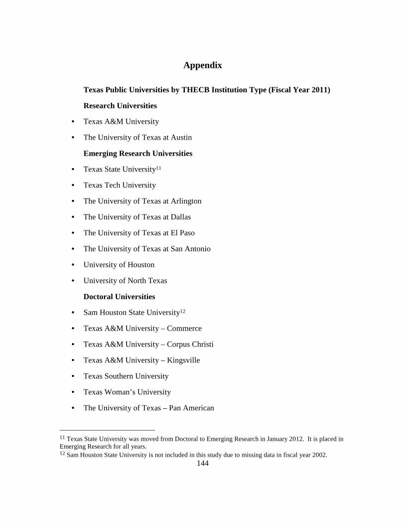
144

Appendix

Texas Public Universities by THECB Institution Type (Fiscal Year 2011)

Research Universities

• Texas A&M University

• The University of Texas at Austin

Emerging Research Universities

• Texas State University11

• Texas Tech University

• The University of Texas at Arlington

• The University of Texas at Dallas

• The University of Texas at El Paso

• The University of Texas at San Antonio

• University of Houston

• University of North Texas

Doctoral Universities

• Sam Houston State University12

• Texas A&M University – Commerce

• Texas A&M University – Corpus Christi

• Texas A&M University – Kingsville

• Texas Southern University

• Texas Woman’s University

• The University of Texas – Pan American

11 Texas State University was moved from Doctoral to Emerging Research in January 2012. It is placed in Emerging Research for all years. 12 Sam Houston State University is not included in this study due to missing data in fiscal year 2002.

145

Comprehensive Universities

• Lamar University-Beaumont

• Prairie View A&M University

• Stephen F. Austin University

• Texas A&M International University

• West Texas A&M University

Master’s Universities

• Angelo State University

• Midwestern State University

• Sul Ross State University

• Sul Ross University – Rio Grande13

• Texas A&M University-Galveston

• Texas A&M University-Texarkana

• The University of Texas at Brownsville14

• The University of Texas at Tyler

• The University of Texas of the Permian Basin

• University of Houston- Clear Lake

• University of Houston- Downtown

• University of Houston- Victoria

13 Sul Ross University – Rio Grande is included in Sul Ross University data in IPEDS. 14 The University of Texas at Brownsville is excluded from this analysis due to its unique taxation and facility sharing arrangements with the local community college district (Texas Southmost College).

146

References

Adams, C. R., Hankins, R. L., & Schroeder, R. G. (1978). The literature of cost and cost analysis in higher education. In R. L. Hankins & R. G. Schroeder (Eds.), A study of cost analysis in higher education (Vol. 1). Washington, DC: American Council of Education.

Archibald, R. B., & Feldman, D. H. (2006). Explaining Increases in Higher Education Costs (Working Paper Number 42). Williamsburg, VA: College of William and Mary, Department of Economics.

Archibald, R. B., & Feldman, D. H. (2007). Avoiding tunnel vision in the study of higher education costs (Working Paper Number 53). Williamsburg, VA: College of William and Mary, Department of Economics.

Badgley, P. (2000a, July 20). Deregulation of U. Texas tuition causes concern, Daily Texan. Retrieved from www.lexisnexis.com

Badgley, P. (2000b, July 11). U. Texas regents push deregulation, Daily Texan. Retrieved from www.lexisnexis.com

Balassa, B. (1964). The purchasing-power parity doctrine: A reappraisal. The Journal of Political Economy, 72(6), 584-596.

Baumol, W. J. (1967). Macroeconomics of unbalanced growth: The anatomy of urban crisis. The American Economic Review, 57(3), 415-426.

Baumol, W. J. (1996). Children of performing arts, the economic dilemma: The climbing costs of health care and education. Journal of Cultural Economics, 20(3), 183-206.

Baumol, W. J. (2012). The cost disease: Why computers get cheaper and health care doesn't. New Haven, CT: Yale University Press.

Baumol, W. J., & Batey Blackman, S. A. (1995). How to think about rising college costs. Planning for Higher Education, 23(4), 1-7.

Baumol, W. J., Batey Blackman, S. A., & Wolff, E. N. (1985). Unbalanced growth revisited: Asymptotic stagnancy and new evidence. The American Economic Review, 75(4), 806-817.

Baumol, W. J., & Bowen, W. G. (1966). Performing arts, the economic dilemma. New York, NY: Twentieth Century Fund.

Bell, C. S. (1968). Macroeconomics of unbalanced growth: Comment. The American Economic Review, 58(4), 877-884.

Bello, R. (2000, September 20). Commission evaluates tuition deregulation, Daily Texan. Retrieved from www.lexisnexis.com

Benton, J. (2003, March 14). Texas bills address state-university tuition rates, Dallas Morning News. Retrieved from www.lexisnexis.com

Berdahl, R. O. (1985). Strategy and government: U.S. state systems and institutional role and mission. International Journal of Institutional Management in Higher Education, 9(3), 301-307.

Besharov, G. (2005). The outbreak of the cost disease: Baumol and Bowen's founding of cultural economics. History of Political Economy, 37(3), 412-430.

147

Bowen, H. R. (1970). Financial needs of the campus. Proceedings of the Academy of Political Science, 30(1), 75-93.

Bowen, H. R. (1980). The costs of higher education. Washington, DC: Jossey-Bass. Bowen, W. G. (2012). Costs and productivity in higher education The Tanner Lectures.

New York, NY: ITHAKA. Bowerman, B. L., & O'Connell, R. T. (1993). Forecasting and time series. North

Scituate, MA: Duxbury. Box, G. E. P., Jenkins, G. M., & Reinsel, G. C. (1994). Time series analysis, forecasting

and control (3rd. ed.). Englewood Cliffs, NJ: Prentice Hall. Breneman, D. W. (2001). An essay on college costs Study of college costs and prices,

1988-89 to 1997-98 (Vol. 2: Commissioned Papers). Washington, DC: National Center for Education Statistics.

Brinkman, P. T. (1981). Factors affecting instructional costs at major research universities. Journal of Higher Education, 52(3), 265-279.

Brinkman, P. T. (1990). Higher education cost functions. In S. Hoenack & E. Collins (Eds.), The economics of American universities (pp. 107-129). New York, NY: State University of New York Press.

Burck, R. D. (2001, January 11). Texas needs to deregulate higher education, Editorial, Austin-American Statesman. Retrieved from www.lexisnexis.com

Chen, C. (2002, April 14-17). Robust regression and outlier detection with the ROBUSTREG procedure. Paper presented at the Sas Users Group International 27, Orlando, Florida.

Cohn, E., Rhine, S. L. W., & Santos, M. C. (1989). Institutions of higher education as multi-product firms: Economies of scale and scope. The Review of Economics and Statistics, 71(2), 284-290.

Conner, T. W., & Rabovsky, T. M. (2011). Accountability, affordability, access: A review of the recent trends in higher education policy research. Policy Studies Journal, 39(s1), 93-112.

Cowen, T. (1996a). Do artists suffer from a cost-disease? Rationality and Society, 8(1), 5-24.

Cowen, T. (1996b). Why I do not believe in the cost-disease: Comment on Baumol. Journal of Cultural Economics, 20(3), 207-214.

Dickeson, R. C. (2006). Frequently asked questions about college costs. Washington, DC: U. S. Department of Education, The Secretary of Education's Commission on the Future of Higher Education.

Dill, D. D., & Soo, M. (2004). Transparency and quality in higher education markets. In P. Teixeira, B. Jongbloed, D. D. Dill & A. Amaral (Eds.), Markets in higher education (pp. 61-86). Dordrecht, The Netherlands: Kluwer.

Douglass, J. A., & Keeling, R. (2008). The big curve: Trends in university fees and financing in the EU and US Research and Occasional Papers Series. Berkeley, CA: University of California at Berkeley.

Drosjack, M. (2003, April 25). University of Texas President lauds tuition bill as 'wise', Houston Chronicle. Retrieved from www.lexisnexis.com

148

Ehrenberg, R. G. (2000). Tuition rising : Why college costs so much. Cambridge, MA: Harvard University Press.

Eisenkopf, G. (2007). Deregulation and customer input in higher education. http://ssrn.com/abstract=881560

Elliott, J. (2002a, December 12). Panel opposes University of Texas System's request to set its own tuition, Houston Chronicle. Retrieved from www.lexisnexis.com

Elliott, J. (2002b, December 11). University of Texas seeks ability to raise tuition, Houston Chronicle. Retrieved from www.lexisnexis.com

Faulkner, L. R. (2004). Address on the state of the university 2004. Retrieved May 25, 2013, from http://www.utexas.edu/news/2004/10/06/nr_university/

Flom, P. L., & Cassell, D. L. (2007, November 11-14). Stopping stepwise: Why stepwise and similar selection methods are bad, and what you should use. Paper presented at the NorthEast SAS User Group, Baltimore, Maryland.

Frenette, M. (2005). The impact of tuition fees on university access: Evidence from a large-scale price deregulation in professional programs. Ottawa, Canada: Statistics Canada

Getz, M., & Siegfried, J. J. (1991). Costs and productivity in American colleges and universities. In C. T. Clotfelter, R. G. Ehrenberg, M. Getz & J. J. Siegfried (Eds.), Economic challenges in higher education. Chicago, IL: University of Chicago.

Greene, W. H. (2010). Econometric analysis (7th Ed.). Upper Saddle River, NJ: Prentice Hall.

Gumport, P. J., & Pusser, B. (1995). A case of bureaucratic accretion: Context and consequences. Journal of Higher Education, 66(5), 493-520.

Harmon, D., & Kay, M. (2003, June 1). Leaders seek to end caps on college tuition, Austin-American Statesman. Retrieved from www.lexisnexis.com

Harter, J. F. R., Wade, J. A., & Watkins, T. G. (2005). An examination of costs at four-year public colleges and universities between 1989 and 1998. The Review of Higher Education, 28(3), 369-391.

Hauptman, A. M. (2001). Reforming the way in which states finance higher education. In D. E. Heller (Ed.), The states and public higher education policy (pp. 64-80). Baltimore, MD: Johns Hopkins University Press.

Heflin, M. (2012). Education, research, and spending decisions. (Unpublished senior thesis). University of Puget Sound, WA.

Heller, D. E. (2001). Trends in the affordability of public colleges and universities. In D. E. Heller (Ed.), The states and higher education policy (pp. 11-38). Baltimore: Johns Hopkins University.

Herman, K. (2003, February 12). Governor unveils budget recipe, Austin-American Statesman. Retrieved from www.lexisnexis.com

Hernandez, J. C. (2009). Student price response: The effect of tuition deregulation in Texas on student enrollment trends in Texas public institutions of higher education. (Doctoral dissertation). (UMI No. 3358873).

149

Holmstrom, B., & Milgrom, P. (1991). Multitask principal-agent analyses: Incentive contracts, asset ownership, and job design. Journal of Law, Economics, & Organization, 7(Special Issue), 24-52.

Horchle, D. (2007). Robust standard errors for panel regressions with cross-sectional dependence. The Stata Journal, 7(3), 281-312.

Huber, P. J. (1964). Robust estimation of a location parameter. The Annals of Mathematical Statistics, 35(1), 73-101.

Hübner, M. (2012). Do tuition fees affect enrollment behavior? Evidence from a ‘natural experiment’ in Germany. Economics of Education Review, 31(6), 949-960.

Jayson, S. (2002a, December 14). Free tuition tied to giving Regents power to set rate, Austin-American Statesman. Retrieved from www.lexisnexis.com

Jayson, S. (2002b, December 12). UT brass pushing for tuition control, Austin-American Statesman. Retrieved from www.lexisnexis.com

Jayson, S. (2003a, February 28). UT President revives infrastructure fee idea, Austin-American Statesman. Retrieved from www.lexisnexis.com

Jayson, S. (2003b, February 14). Yudof: Tuition could rise 27 percent Austin-American Statesman. Retrieved from www.lexisnexis.com

Johnstone, D. B. (2001). Higher education and those "out of control costs" Study of college costs and prices, 1988-89 to 1997-98 (Vol. 2: Commissioned Papers). Washington, DC: National Center for Educational Statistics.

Jones, D. P. (2001). Cost analysis and the formulation of public policy Study of college costs and prices, 1988-89 to 1997-98 (Vol. 2: Commissioned Papaers). Washington, DC: National Center for Educational Statistics.

Kay, M. (2003a, April 30). Bill to deregulate tuition advances, Austin-American Statesman. Retrieved from www.lexisnexis.com

Kay, M. (2003b, April 16). Deregulation of tuition out of Senate bill, Austin-American Statesman. Retrieved from www.lexisnexis.com

Kay, M. (2003c, May 21). Tuition deregulation appears dead for now, Austin-American Statesman. Retrieved from www.lexisnexis.com

Kay, M., & Jayson, S. (2003, February 13). State leaders embracing uncapped tuitions, Austin-American Statesman. Retrieved from www.lexisnexis.com

King, G., & Roberts, M. (2015). How robust standard errors expose methodological problems they do not fix. Political Analysis, Advance online publication. doi: 10.1093/pan/mpu015

Kirshstein, R. J., & Hurlburt, S. (2012). Revenues: Where does the money come from? Washington, DC: American Institutes for Research.

Krusell, P., Ohanian, L. E., & Ríos-Rull, J. V. (2000). Capital skill complementarity and inequality: A macroeconomic analysis. Econometrica, 68(5), 1029-1053.

Lane, J. E., & Kivisto, J. A. (2008). Interests, information, and incentives in higher education: Principal-agent theory and its potential applications to the study of higher education governance. In J. C. Smart (Ed.), Higher education: Handbook of theory and research (Vol. XXIII, pp. 141-180). Dordrecht, The Netherlands: Springer.

150

Lasher, W. F., & Sullivan, C. A. (2004). Follow the money: The changing world of budgeting in higher education. In J. C. Smart (Ed.), Higher education: Handbook of theory and research (Vol. XIX, pp. 197-240). Dordrecht, The Netherlands: Kluwer.

Leslie, L. L., Slaughter, S., Taylor, B. J., & Zhang, L. (2011). How do revenue variations affect expenditures within U.S. research universities? Research in Higher Education, 53(6), 614-639.

Lim, Y. (2003, January 28). U. Texas President seeks methods to meet budget cuts, Daily Texan. Retrieved from www.lexisnexis.com

Lingenfelter, P. E. (2006). The un-funding of higher education ??? Retrieved May 26, 2013, from http://archive.sheeo.org/about/paulpres/Baruch%20College.pdf

Lowery, D. (2002, September 1). An educated Texas is a prosperous Texas, Editorial, Austin-American Statesman. Retrieved from www.lexisnexis.com

Martin, R. E. (2009). The revenue-to-cost spiral in higher education. Raleigh, NC: John W. Pope Center for Education Policy.

Martin, R. E. (2011). The college cost disease: Higher cost and lower quality. Northampton, MA: Edward Elgar.

Martin, R. E. (2012). Higher education governance as a barrier to cost containment. Paper presented at the Stretching the Higher Education Dollar conference, Washington, DC.

Martin, R. E., & Hill, R. C. (2012). Measuring Baumol and Bowen effects in public research universities. http://ssrn.com/abstract=2153122

Massy, W. F., & Wilger, A. K. (1992). Productivity in postsecondary education: A new approach. Education Evaluation and Policy Analysis, 14(4), 361-376.

Middaugh, M. F., Graham, R., & Shahid, A. (2003). A study of higher education instructional expenditures: The Delaware study of instructional costs and productivity. Washington, DC: National Center for Educational Statistics.

Mock, J. (2002, April 17). U. Texas Regents want systems to present unified front, Daily Texas. Retrieved from www.lexisnexis.com

Morphew, C. C., & Baker, B. D. (2004). The cost of prestige: Do new research one universities incur increased administrative costs? Review of Higher Education, 27(3), 365-384.

Mumper, M. (2003). The future of college access: The declining role of public higher education in promoting equal opportunity. The Annals of the American Academy of Political and Social Science, 585, 97-117.

Nelson, P. (1970). Information and consumer behavior. Journal of Political Economy, 78(2), 311-329.

Newey, W. K., & West, K. D. (1987). A simple, positive semi-definite, heteroskedasticity and autocorrelation consistent covariance matrix. Econometrica, 55(3), 703-708.

Nissimov, R. (2002, March 6). Giant fee hike at University of Texas results in apology, legal confusion, Houston Chronicle. Retrieved from www.lexisnexis.com

Nordhaus, W. D. (2008). Baumol's diseases: A macroeconomic perspective. The B. E. Journal of Macroeconomics, 8(1), 1-37.

151

O'Meara, K. (2007). Striving for what? Exploring the pursuit of prestige. In J. C. Smart (Ed.), Higher education: Handbook of theory and research (Vol. XXII, pp. 121-179). Dordrecht, The Netherlands: Springer.

Petersen, M. A. (2009). Estimating standard errors in finance panel data sets: Comparing approaches. The Review of Financial Studies, 22(1), 435-480.

Preston, P., & Sparviero, S. (2009). Creative inputs as the cause of Baumol's cost disease: The example of media services. Journal of Media Economics, 22(4), 239-252.

Reisman, D. (1956). Constraint and variety in American education. Lincoln, NB: University of Nebraska Press.

Reynolds, A. (1998). The real cost of higher education, who should pay it, and how? Report of the National Commission on the Cost of Higher Education. Washington, DC: National Center for Education Statistics.

Rothstein, J., & Rouse, C. E. (2010). Constrained after college: Student loans and early-career occupational choices. Journal of Public Economics, 95(1-2), 149-163.

Samuelson, P. (1964). Theoretical notes on trade problems. Review of Economics and Statistics, 23(2), 145-154.

Stone, R. (2001, June 5). Actions of Legislature draw mixed reactions from U. Texas officials, Daily Texas. Retrieved from www.lexisnexis.com

Strein, C. T., & McMahon, W. W. (1979). The university as a non-profit discretionary firm. Urbana, IL: University of Illinois.

Swail, W. S., & Heller, D. E. (2004). Changes in tuition policies: Natural policy experiments in five countries. Montreal, QC, Canada: Canada Millennium Scholarship Foundation.

Texas Higher Education Coordinating Board. (2010). Overview tuition deregulation. Retrieved November 10, 2012, from http://www.thecb.state.tx.us/reports/PDF/1527.PDF

Tibshirani, R. (1996). Regression shrinkage and selection via the LASSO. Journal of the Royal Statistical Society. Series B (Methodological), 58(1), 267-288.

Tinto, V. (1987). Leaving college : Rethinking the causes and cures of student attrition. Chicago: University of Chicago Press.

Titus, M. (2009). The production of bachelor's degrees and financial aspects of state higher education policy: A dynamic analysis. Journal of Higher Education, 80(4), 439-468.

Triplett, J. E., & Bosworth, B. (2003). Productivity measurement issues in service industries: "Baumol's disease" has been cured. Economic Policy Review, 9(3), 23-33.

White, H. (1980). A heteroskedasticity-consistent covariance matrix estimator and a direct test for heteroskedasticity. Econometrica, 48(4), 817-838.

Wildavsky, A. (1961). Political implications of budgetary reform. Public Administration Review, 21(1), 183-190.

Winston, G. C. (1998). College cost: Subsidies, intuition, and policy Report of the National Commission on the Cost of Higher Education. Washington, DC: National Center for Educational Statistics.

152

Winston, G. C. (1999). Subsidies, hierarchy, and peers: The awkward economics of higher education. Journal of Economic Perspectives, 13(1), 13-36.

Winston, G. C. (2000). The positional arms race in higher education (Discussion Paper No. 54). Williamstown, MA: Williams College.

Wolf, D. F. (2004). Survey of Texas public universities and university systems involvement in state public policy making. (Doctoral dissertation). (UMI No. 3145019).

Yohai, V. (1987). High breakdown-point and high efficiency robust estimates for regression. The Annals of Statistics, 15(2), 642-656.

Zeileis, A. (2004). Econometric computing with HC and HAC covariance matrix estimators. Journal of Statistical Software, 11(10), 1-16.

153

Vita

George Purcell was born in New Orleans, Louisiana and grew up in Kansas City,

Missouri. He received a Bachelor of Science in Political Science from Truman State

University in 1995, a Master of Arts in International Relations from the Australian

National University in 1997, and a Master of Public Affairs from the Lyndon Baines

Johnson School at the University of Texas at Austin in 1998. He was a Fulbright Scholar

to Australia in 1996. He entered the Ph.D. program in Government at the University of

Texas at Austin in 1998 and transferred to the Department of Educational Administration

in 2006. From 2002 through 2005, he was the Director of Research and Evaluation at the

Center for State Scholars. Since 2005, he has been an analyst focusing on higher

education policy and finance at the Texas Legislative Budget Board (LBB). The analysis

contained in this research does not represent the position of the LBB and has not been

subject to agency review.

Address: [email protected]

This dissertation was typed by the author.

copyright by george phillip purcell, jr. 2015

Documents