coordination of independent learners in cooperative markov

HAL Id: hal-00370889https://hal.archives-ouvertes.fr/hal-00370889

Preprint submitted on 25 Mar 2009

HAL is a multi-disciplinary open accessarchive for the deposit and dissemination of sci-entific research documents, whether they are pub-lished or not. The documents may come fromteaching and research institutions in France orabroad, or from public or private research centers.

L’archive ouverte pluridisciplinaire HAL, estdestinée au dépôt et à la diffusion de documentsscientifiques de niveau recherche, publiés ou non,émanant des établissements d’enseignement et derecherche français ou étrangers, des laboratoirespublics ou privés.

Coordination of independent learners in cooperativeMarkov games.

Laëtitia Matignon, Guillaume J. Laurent, Nadine Le Fort-Piat

To cite this version:Laëtitia Matignon, Guillaume J. Laurent, Nadine Le Fort-Piat. Coordination of independent learnersin cooperative Markov games.. 2009. �hal-00370889�

https://hal.archives-ouvertes.fr/hal-00370889

https://hal.archives-ouvertes.fr

Institut FEMTO-ST

Universite de Franche-Comte

Coordination of independent learners in cooperative

Markov games

Laetitia Matignon, Guillaume J. Laurent and Nadine Le Fort-Piat

Rapport technique / Technical Report

2009

Institut FEMTO-STUMR CNRS 6174 — UFC / ENSMM / UTBM

32 avenue de l’Observatoire — 25044 BESANCON Cedex FRANCETel : (33 3) 81 85 39 99 — Fax : (33 3) 81 85 39 68

email : [email protected]

Abstract

In the framework of fully cooperative multi-agent systems, independent agents learningby reinforcement must overcome several difficulties as the coordination or the impact ofexploration. The study of these issues allows first to synthesize the characteristics of ex-isting reinforcement learning decentralized methods for independent learners in cooperativeMarkov games. Then, given the difficulties encountered by these approaches, we focus ontwo main skills: optimistic agents, which manage the coordination in deterministic envi-ronments, and the detection of the stochasticity of a game. Indeed, the key difficulty instochastic environment is to distinguish between various causes of noise. The SOoN al-gorithm is so introduced, standing for “Swing between Optimistic or Neutral”, in whichindependent learners can adapt automatically to the environment stochasticity. Empiricalresults on various cooperative Markov games notably show that SOoN overcomes the mainfactors of non-coordination and is robust face to the exploration of other agents.

1 Introduction

Over the last decade, many approaches are concerned with the extension of RL to multi-agentsystems (MAS) [1]. On the one hand, adopting a decentralized point of view with MAS offersseveral potential advantages as speed-up, scalability and robustness [2]. On the other hand,reinforcement learning (RL) methods do not need any a priori knowledge about the dynamicsof the environment, which can be stochastic and non linear. An agent interacting with itsenvironment tests different actions and learns a behavior by using a scalar reward signal calledreinforcement as performance feedback. Modern RL methods rely on dynamic programmingand have been studied extensively in single-agent framework [3]. By using RL in MAS, theiradvantages can be associated : autonomous and “simple” agents can learn to resolve in adecentralized way complex problems by adapting to them.

However, there are still many challenging issues in applying RL to MAS [4]. For instance,one difficulty is the loss of theoretical guarantees. Indeed convergence hypothesis of single-agent framework are no longer satisfied. Another matter is that the computation complexityof decentralized MAS often grows exponentially with the number of agents [5, 6, 7]. Finally,a fundamental difficulty faced by agents that work together is how to efficiently coordinatethemselves [8, 9, 10]. MAS are qualified by a decentralized execution, so each agent takesindividual decisions but all of the agents contribute globally to the system evolution. Learningin MAS is then more difficult since the selection of actions must take place in the presence ofother learning agents. A study of some mis-coordination factors is proposed in this report.

Despite these difficulties, several successful applications of decentralized RL have been re-ported, like the control of a group of elevators [11] or adaptative load-balancing of parallelapplications [12]. Air traffic flow management [13] and data transportation by a constellationof communication satellites [14] are other examples of real world applications of cooperativeagents using RL algorithms. We have an interest in practical applications in robotics, wheremultiple cooperating robots are able to complete many tasks more quickly and reliably thanone robot alone. Especially, the real world objective of our work is the decentralized controlof a distributed micro-manipulation system based on autonomous distributed air-flow MEMS1,called smart surface [15]. It consists of an actuators array on which an object is situated. Theobjective is for the hundreds of actuators to choose from a small set of actions over many trialsso as to achieve a common goal.

We focus here on learning algorithm in cooperative MAS [16] which is a fitting model forsuch a real world scenario. Especially, in this report, we are interested in the coordination of

1Micro Electro Mechanical Systems.

1

adaptative and cooperative agents with the assumption of a full individual state observability.We consider independent learners (ILs) which were introduced in [17] as agents which don’tknow the actions taken by the other agents. The choice of ILs is particularly pertinent givenour objective of robotic applications with numerous agents, where the assumption of joint actionobservability required for the joint action learners is hard to satisfy.

Our objective is to develop an easy-to-use, robust and decentralized RL algorithm for au-tonomous and independent learners in the framework of cooperative MAS. The chosen frame-work is cooperative Markov games. One of our contribution is to analyse what is at stake inthe learning of ILs in this framework. Thanks to this study, we synthesize the characteristics ofexisting RL decentralized methods for ILs in cooperative Markov games. Then, we introducea new algorithm named the SOoN algorithm, standing for “Swing between Optimistic or Neu-tral”, in which ILs can adapt automatically to the environment stochasticity. We successfullydevelop this algorithm thanks to our analysis of previous algorithms and apply it within vari-ous matrix games and Markov games benchmarks. Its performance is also compared to otherlearning algorithms.

The report is organized as follows. In section 2, our theoretical framework is described.Learning in MAS has strong connections with game theory so a great part of the report concernsrepeated matrix games. Matrix games study is a necessary first step toward the framework ofMarkov games. Indeed, it allows a better understanding of mis-coordination issues, presented insection 3 as one of major stakes of ILs in cooperative MAS. We overview related algorithms insection 4 and provide a uniform notation that has never been suggested and which emphasizescommon points between some of these algorithms. This leads to a recursive version of theFMQ algorithm in the matrix game framework (section 6). It is successfully applied on matrixgames which contain hard coordination challenges. Finally, in section 7, we present the SOoNalgorithm in the general class of Markov games and show results demonstrating its robustness.

2 Theoretical framework

The studies of reinforcement learning algorithms in MAS are based on Markov games whichdefine multi-agent multi-state models. They are the synthesis of two frameworks : Markovdecision processes and matrix games. Markov decision processes are a single-agent multi-statemodel explored in the field of RL. Matrix games, on the other hand, are a multi-agent single-state model used in the field of game theory. These frameworks are independently consideredin this section. In addition, some classifications and equilibrium concepts are outlined.

2.1 Markov Decision Processes

Definition 1 A Markov Decision Process (MDP) [18, 19] is a tuple < S,A, T,R > where :

• S is a finite set of states;

• A is a finite set of actions;

• T : S × A× S �→ [0; 1] is a transition function that defines a probability distribution overnext states. T (s, a, s′) is the probability of reaching s′ when the action a is executed in s,also noted P (s′|s, a),

• R : S × A × S �→ R is a reward function giving the immediate reward or reinforcementreceived under each transition.

2

At each time step, the agent chooses an action at that leads the system from the state st to thenew state st+1 according to a transition probability T (st, at, st+1). Then it receives a rewardrt+1 = R(st, at, st+1). Solving MDPs consists in finding a mapping from states to actions, calleda policy π : S × A �→ [0; 1], which maximizes a criterion. π(s, a) is the probability of choosingthe action a in state s. Most of single agent RL algorithms are placed within this framework[20, 21, 3].

2.2 Matrix games

Game theory is commonly used to analyze the problem of multi-agent decision making, where agroup of agents coexist in an environment and take simultaneous decisions. We first define thematrix game framework and the classification of these games, and then we examine two mainequilibrium concepts.

2.2.1 Definition and strategy

Definition 2 A matrix game2 [22, 23] is a multiple agent, single state framework. It is definedas a tuple < m,A1, ..., Am, R1, ..., Rm > where :

• m is the number of players;

• Ai is the set of actions available to player i (and A = A1 × ... × Am is the joint actionspace);

• Ri : A �→ R is player i’s reward or payoff function.

The goal of a learning agent in a matrix game is to learn a strategy that maximizes its reward.In matrix games, a strategy3 πi : Ai �→ [0; 1] for an agent i specifies a probability distributionover actions, i.e. ∀ai ∈ Ai πi(ai) = P (ai). π is the joint strategy for all of the agents and π−i

the joint strategy for all of the agents except agent i. We will use the notation 〈πi,π−i〉 to referto the joint strategy where agent i follows πi while the other agents follow their policy fromπ−i. Similarly, A−i is the set of actions for all of the agents except agent i. The set of all ofthe strategies for the agent i is noted ∆(Ai).

2.2.2 Type of matrix games

Matrix games can be classified according to the structure of their payoff function. If payofffunctions sum is zero, the game is called fully competitive game4. If all agents have the samepayoff function, i.e. R1 = ... = Rm = R, the game is called fully cooperative game5. Finally, ingeneral-sum game, the individual payoffs can be arbitrary.

In this paper, we focus on fully cooperative game. In these games, an action in the bestinterest of one agent is also in the best interest of all agents. Especially, we are interested inrepeated games which consist of the repetition of the same matrix game by the same agents.

The game in table 1 depicts a team game between two agents which is graphically representedby a payoff matrix. The rows and columns correspond to the possible actions of respectivelythe first and second agent, while the entries contain the payoffs of the two agents for thecorresponding joint action. In this example, each agent chooses between two actions a and b.Both agents receive a payoff of 0 when both selected actions of the agents differ, and a payoffof 1 or 2 when the actions are the same.

2also called strategic game.3also called policy.4also called zero-sum game.5also called team game or identical payoff game.

3

Table 1: Fully cooperative game example.Agent 2a b

Agent 1 a 2 0b 0 1

2.2.3 Equilibria

First, we define the expected gain for an agent i as the expected reward given its strategy andthe strategies of others.

Definition 3 The expected gain for an agent i given a joint strategy π = 〈πi,π−i〉, noted ui,π,is :

ui,π = Eπ {Ri(a)} =∑a∈A

π(a)Ri(a). (1)

From a game-theoretic point of view, two common concepts of equilibrium are used to defineoptimal solutions in games. The first one is called Nash equilibrium [24, 23].

Definition 4 A joint strategy π∗ defines a Nash equilibrium iff, for each agent i, there is :

∀πi ∈ ∆(Ai) ui,〈π∗i ,π∗

−i〉 ≥ ui,〈πi,π∗−i〉. (2)

Thus, no agent can improve its payoff by unilaterally deviating from a Nash equilibrium. Amatrix game can have more than one Nash equilibrium. For example, the matrix game in table1 has two Nash equilibria corresponding to the joint strategies where both agents select thesame action. However, a Nash equilibrium is not always the best group solution. That’s whythe Pareto optimality has been defined.

Definition 5 A joint strategy π Pareto dominates another joint strategy π iff :

• each agent i following πi receives at least the same expected gain as with πi and,

• at least one agent j following πj receives a strictly higher expected gain than with πj,

that’s to say formally :

π > π ⇔ ∀i ui,π ≥ ui,π and ∃j uj,π > uj,π. (3)

Definition 6 If a joint strategy π∗ is not Pareto dominated by any other joint strategy, thenπ∗ is Pareto optimal.

So a Pareto optimal solution is one in which no agent’s expected gain can be improved uponwithout decreasing the expected gain of at least one other agent. There are many examples ofgeneral-sum games where a Pareto optimal solution is not a Nash equilibrium and vice-versa (forexample, the prisoner’s dilemma). However, in fully cooperative games, each Pareto optimalsolution is also a Nash equilibrium by definition. This means that if a joint action provides oneagent with maximal possible reward, it must also maximise the reward received by the otheragents. For instance in the matrix game of the table 1, the joint strategy 〈a, a〉 defines a Paretooptimal Nash equilibrium.

4

2.3 Markov games

Markov games can be seen as the extension of matrix games to the multiple states framework.Specifically, each state of a Markov game can be viewed as a matrix game. Another point ofview is to consider Markov games as an extension of MDP to multiple agents. Markov gameswere first examined in the field of game theory and more recently in the field of multi-agent RL.

2.3.1 Definition

Definition 7 A Markov game6 [25] is defined as a tuple < m,S,A1, ..., Am, T,R1, ..., Rm >where :

• m is the number of agents;

• S is a finite set of states;

• Ai is the set of actions available to the agent i (and A = A1 × ... × Am the joint actionspace);

• T : S × A × S �→ [0; 1] a transition function that defines transition probabilities betweenstates;

• Ri : S ×A �→ R the reward function for agent i.

In Markov game framework, all agents have access to the complete observable state s. The tran-sition and reward functions are functions of the joint action. An individual policy πi : S×Ai �→[0; 1] for an agent i specifies a probability distribution over actions, i.e. ∀ai ∈ Ai P (ai|s) =πi(s, ai). The set of all of the policies for the agent i is noted ∆(S,Ai). If for an agent i and forall states s, πi(s, ai) is equal to 1 for a particular action ai and 0 for the others, then the policyπi is called a pure policy.

The same classification for matrix games can be used with Markov games. If all agentsreceive the same rewards, the Markov game is fully cooperative. It is then defined as anidentical payoff stochastic game (IPSG)7 [26].

2.3.2 Equilibria

As in matrix games, we can define for each state s the immediate expected gain for an agent ifollowing the joint strategy π as :

ui,π(s) = Eπ {Ri(s, a)} =∑a∈A

π(s, a)Ri(s, a). (4)

Thus, the long term expected gain from the state s for an agent i is, when all the agents followπ :

Ui,π(s) = Eπ

{ ∞∑k=0

γkui,π(s)t+k+1|st = s

}(5)

where γ ∈ [0; 1] is a discount factor.The concepts of Nash equilibrium and Pareto optimality are also defined in Markov games.

6also called stochastic game.7also called Multi-agent Markov Decision Process (MMDP).

5

Definition 8 A joint policy π∗ defines a Nash equilibrium in a Markov game iff, for each agenti, there is :

∀πi ∈ ∆(S,Ai) ∀s ∈ S Ui,〈π∗i ,π∗

−i〉(s) ≥ Ui,〈πi,π∗−i〉(s). (6)

Definition 9 A joint policy π Pareto dominates another joint policy π iff, in all states :

• each agent i following πi receives at least the same expected gain as with πi and,

• at least one agent j following πj receives a strictly higher expected gain than with πj,

that’s to say formally :

π > π ⇔ ∀i, ∀s ∈ S Ui,π(s) ≥ Ui,π(s) et ∃j Uj,π(s) > Uj,π(s). (7)

Definition 10 If a joint policy π∗ is not Pareto dominated by any other joint strategy, thenπ∗ is Pareto optimal.

2.4 Conclusion

In this paper, we are interested in cooperative games, where we defined the objective as findinga Pareto-optimal Nash equilibrium, also called optimal equilibrium. Indeed, the policies whichdefine Pareto-optimal Nash equilibria maximise the expected sum of the discounted rewards inthe future for all agents. However, there can be several Pareto-optimal Nash equilibria so somecoordination mechanisms on a single equilibrium are necessary.

3 The independent learners coordination problem

The main difficulty in the cooperative independent learners (ILs) framework is the coordinationof ILs : how to make sure that all agents coherently choose their individual action such thatthe resulting joint action is optimal? We analyze this problem using the framework of fullycooperative matrix games that we have introduced in section 2.2. Each agent independently hasto select an action from its action set. It receives a payoff based on the resulting joint action.Formally, the challenge in multi-agent RL is to guarantee that the individual optimal policiesπ∗i define an optimal joint policy π∗ [27], i.e. a Pareto-optimal Nash equilibrium.

The coordination is a complex problem which arises from the combined action of severalfactors. In large games, it is hard to identify these factors since they are often combinedwith other phenomena. So the classification proposed here is probably not exhaustive. Itresults from a study of matrix games with a small number of agents, where the identificationand interpretation of some factors are more obvious. Of course, the exposed factors can beadapted to games with many agents and to Markov games. These factors make the analysisand development of coordination techniques in RL algorithms easier.

Fulda and Ventura [8] identify two main factors : shadowed equilibrium and equilibria selec-tion problems that we formalized here. We also add two other factors : the noise in the gameand the impact of the exploration of other agents on the learning of one agent.

3.1 Shadowed equilibrium

Definition 11 An equilibrium defined by a strategy π is shadowed by a strategy π iff :

∃i ∃πi u〈πi,π−i〉 < minj,πj

u〈πj ,π−j〉 (8)

6

Table 2: Simple cooperative matrix game.Agent 2a b c

a 5 3 1Agent 1 b 4 1 1

c 1 1 0

Table 3: The Climbing game and the Penalty game have been introduced in [28] and partiallyand fully stochastic variations of the Climbing game, proposed in [29]. In stochastic games, theprobability of each reward is 50%.

(a) Climbing game (b) Partially stochastic Climbing gameAgent 2

a b c

a 11 -30 0Agent 1 b -30 7 6

c 0 0 5

Agent 2a b c

a 11 -30 0Agent 1 b -30 14/0 6

c 0 0 5

(c) Fully stochastic Climbing game (d) Penalty game (k ≤ 0)Agent 2

a b c

a 10/12 5/-65 8/-8Agent 1 b 5/-65 14/0 12/0

c 8/-8 12/0 10/0

Agent 2a b c

a 10 0 kAgent 1 b 0 2 0

c k 0 10

7

A particular structure game could be a game with a shadowed Pareto optimal Nash equilib-rium. For instance, in the Climbing game (table 3), the Pareto optimal Nash equilibrium 〈a, a〉and the sub-optimal Nash equilibrium 〈b, b〉 are shadowed because penalties are associated tomis-coordination on 〈a, b〉 or 〈b, a〉. Moreover, there are no mis-coordination penalties associ-ated with action c, potentially making it tempting for the agents. The joint action 〈c, c〉 is theonly unshadowed equilibrium in the Climbing game. So 〈c, c〉 is potentially interesting for ILs.

3.2 Equilibria selection problems

The equilibria selection problem takes place whenever at least two agents are required to selectbetween multiple Pareto optimal Nash equilibria. In this case, some agents must choose betweenseveral optimal individual policies but only some combinations of these optimal individual poli-cies define an optimal equilibrium. So the equilibria selection problem can be defined as thecoordination of individual policies so that the resulting joint policy is optimal.

Craig Boutilier introduced the set of potentially individually optimal (PIO) actions for agenti at state s as those actions in Ai that belong to at least one of the optimal joint actions fors [30]. An optimal joint action is a pure joint policy which defines a Pareto optimal Nashequilibrium. This set is denoted PIO(i, s). State s is said to be weakly dependent for agent iif there is more than one PIO choice for i at s. We can define the equilibria selection problemwith this notion.

Definition 12 There is an equilibria selection problem at state s if at least two agents arerequired to select between multiple Pareto optimal Nash equilibria at this state, i.e. s is weaklydependent for at least two agents.

The Penalty game (table 3d) is usually chosen to illustrate the equilibria selection problem.There are two Pareto optimal Nash equilibria : 〈a, a〉 and 〈c, c〉 and one sub-optimal Nashequilibrium 〈b, b〉. The set of potentially individually optimal actions for each agent is then{a, c}. So the Penalty game is weakly dependent for the two agents and agents confront anequilibria selection problem. Simply choosing an individual optimal action in the set PIO doesnot guarantee that the resulting joint action will be optimal since four joint actions are thenpossible (〈a, a〉, 〈c, c〉, 〈a, c〉, 〈c, a〉) and only two of them are optimal.

In this game, k is usually chosen inferior to 0 so as to combine shadowed equilibria withequilibria selection issue. Indeed, the only unshadowed equilibrium in this game is the sub-optimal Nash equilibrium 〈b, b〉.

3.3 Noise in the environment

Agents in a MAS can be confronted with noise in their environment. Noise in the environmentcan be due to various phenomena : stochastic rewards, e.g. in the stochastic variations ofthe Climbing game (table 3d and c), unobservable factors in the state space, uncertainty, ... .However, changing behaviors of the other agents can also be interpreted as noise by an IL. Forinstance in the partially stochastic Climbing game, an IL must distinguish if distinct rewardsreceived for the action b are due to various behaviors of the other agent or to stochastic rewards.The agent must learn that the average reward for the joint action 〈b, b〉 is 7 and is lower than thatof 〈a, a〉. Thus the difficulty in ILs games is to distinguish between noise due to the environmentand noise due to other agents behaviors. This behavior is notably characterized by actions ofexploration.

8

3.4 Exploration

In MAS as in single-agent case, each IL must choose actions of exploration or exploitationaccording to its decision strategy. The common action decision called softmax is based onagent’s individual policy πi computed thanks to a Boltzman distribution :

πi(s, a) =e

Qi(s,a)

τ∑u∈Ai

eQi(s,u)

τ

(9)

where τ is the temperature parameter that decreases the amount of randomness as it approacheszero. The ε-greedy strategy is another common action selection method in which an agent fol-lows its greedy policy8 with probability (1 − ε) (exploitation mode), and otherwise selects auniformly random action with probability ε (exploration mode).

The exploration is a major stake in the reinforcement learning of ILs. Indeed, as statedbefore, an IL cannot detect the change of behaviors of the other agents. So the exploration ofothers can induce noise in received rewards of an IL.

So as to quantify the noise due to the exploration in a game, the concept of global explorationmust be pointed out. The global exploration is the probability of having at least one agent whichexplores. It can be formulated with the individual exploration of each agent.

Property 1 Let a n-agents system in which each agent explores according to a probability ε.Then the probability of having at least one agent which explores is ψ = 1− (1− ε)n. ψ is namedglobal exploration.

The exploration of an agent can have strong influences on the learned policy of an IL. In agame with an optimal shadowed equilibrium defined by a policy π, let agent i follow its optimalindividual policy πi. The exploration of others can then lead to penalties (equation 8). So theexploration of others has an influence on the learning of i’s individual policy. Moreover, it cancause the “destruction” of the optimal policy of an IL. So it is necessary that RL algorithmsshould be robust face to exploration.

3.5 Conclusion

In this report, we focus our study on cooperative independent learners. In such a framework,the main issue is to manage the coordination of the learners. We have detailed four factorsresponsible of the non-coordination of agents. Solving these difficulties and overcoming mis-coordination factors is one the main objectives of RL algorithms in MAS. Another key parameteris the robustness face to exploration.

4 Related works in Reinforcement Learning

Various approaches have been proposed in the literature to prevent coordination problems inmulti-independent-learners systems. In this section, related works dealing with RL algorithmsare reviewed with an emphasis on algorithms dealing with Q-learning [31] and Q-learning vari-ants for ILs. We propose a uniform notation, that has never been suggested for these algorithms,and which stresses common points between some of them. For each algorithms, the robustnessface to mis-coordination factors and exploration is discussed.

8A greedy policy based on Qi is to select in a state s the action a for which Qi(s, a) is highest.

9

Table 4: Percentage of trials which converged to the optimal joint action (averaged over 1000trials). A trial consists of 3000 repetitions of the game. At the end of each trial, we determineif the greedy joint action is the optimal one. Results were obtained with softmax decision andvarious exploration strategies : stationary (τ) or GLIE (τ = τini × δt where t is the repetitionsnumber).

Stationary strategy τ = 1000 τ = 200 τ = 10 τ = 1Penalty game (k = −100) 62, 6% 65, 3% 62, 8% 65, 1%

GLIE τini = 5000 τini = 500 τini = 100strategy δ = 0.9 δ = 0.99 δ = 0.995 δ = 0.997 δ = 0.995 δ = 0.995

Penalty game (k = −100) 0% 61, 7% 84% 96, 6% 85, 3% 84, 8%

In the following methods, each IL builds its own Qi-table whose size is independent ofthe agents number and linear in function of its own actions. The task is for the agents toindependently choose one action with the goal of maximizing the expected sum of the discountedrewards in the future.

4.1 Decentralized Q-learning

Q-learning [31] is one of the most used algorithm is single-agent framework because of itssimplicity and robustness. That’s also why it was one of the first RL algorithm applied tomulti-agent environments [17]. The update equation for the agent i is :

Qi(s, ai)← (1− α)Qi(s, ai) + α(r + γmaxu∈Ai

Qi(s′, u)) (10)

where s′ is the new state, ai is the agent’s chosen action, r = R(s, 〈ai, a−i〉) the reward received,Qi(s, ai) the value of the state-action for the agent i, α ∈ [0; 1] the learning rate and γ ∈ [0; 1]the discount factor.

Decentralized Q-learning has been applied with success on some applications [32, 33, 34, 35].However, this algorithm has a low robustness face to exploration. Most of works concerningdecentralized Q-learning use a GLIE9 strategy [36] so as to avoid concurrent exploration. Itconsists in avoiding the simultaneous exploration of agents, namely the concurrent exploration.The principle is to decrease the exploration frequency as the learning goes along so that eachagent should find the best response to the others behaviors. This method is investigated inMAS [28, 37] and section 5.1.

Avoiding concurrent exploration can improved results of some algorithms by allowing ILsto overcome some mis-coordination factors. For instance, results of decentralized Q-learningcan be improved as illustrated on table 4. Best results are obtained with a well chosen GLIEstrategy. However, convergence then relies on the choice of decaying parameters. The use of aGLIE strategy does not ensure convergence to an optimal equilibrium [28] and the key difficultyof this method is that the convergence relies on the choice of decaying parameters. Moreover,setting GLIE parameters requires high skills on algorithm behavior and so it is difficult to applyin real applications.

9Greedy in the limit with infinite exploration.

10

Algorithm 1: Distributed Q-learning for agent i 10

beginInitialization :forall a ∈ Ai and s ∈ S do

Qi,max(s, a)← 0, πi(s, a) arbitrarilys← initial statewhile s is not an absorbing state do

From s select a according to the ε-greedy selection method based on πi

Apply a and observe reward r and next state s′

q ← r + γmaxu∈Ai

Qi,max(s′, u)

if q > Qi,max(s, a) thenQi,max(s, a)← q � optimistic update

if Qi,max(s, arg maxu∈Ai

πi(s, u)) �= maxu∈Ai

Qi,max(s, u) then

Select a random action amax ∈ arg maxu∈Ai

Qi,max(s, u)

∀b ∈ Ai πi(s, b)←{

1 if b = amax

0 else� equilibria selection mechanism

s← s′

end

4.2 Distributed Q-learning

To get round the issue of shadowed equilibria with ILs, Lauer & Riedmiller [38] introduced“optimistic independent agents”. Such agents neglect in their update the penalties which areoften due to a non-coordination of agents. For instance the evaluation of an action in matrixgames is the maximum reward received. In the case of multiple optimal joint actions in a singlestate, an additional procedure for coordination is used to solve the equilibria selection problem.This equilibria selection mechanism is a social convention [30] which places constraints on thepossible action choices of the agents. The central idea is to update the current policy πi only ifan improvement in the evaluation values (Qi,max) happens. This mechanism presents the otherinterest to allow simultaneously the learning of individual policies and exploration. The indi-vidual policies can’t be “destroyed” by exploration since when one of the optimal joint policiesis tried, it is nevermore modified.Distributed Q-learning associated with this equilibria selection method is in algorithm 1. Itaddresses two factors that can cause mis-coordination : shadowed equilibria are preventedthrough the optimistic update and the equilibria selection problem is solved thanks to the equi-libria selection method. It is proved that this algorithm finds optimal policies in deterministicenvironments for cooperative Markov games. Moreover, distributed Q-learning is robust face toexploration. However this approach does generally not converge in stochastic environments.

4.3 Variable learning rate algorithms

To minimize the effect of shadowed equilibria with ILs, some authors propose to minimize theeffect that the learning of other agents has on a given agent’s own learning by using a variablelearning rate. For instance some algorithms based on gradient ascent learners use the Win orLearn Fast (WoLF) heuristic [39] and its variants PD-WoLF [40] or GIGA-WoLF [41]. Othersare based on Q-learning, e.g. the hysteretic Q-learning [42] in which two learning rates α and

11

β are used for the increase and decrease rates of Qi-values. The update equation for the agenti is :

δ ← r + γmaxu∈Ai

Qi(s′, u) (11)

Qi(s, a)←{

(1− α)Qi(s, a) + αδ if δ ≥ Qi(s, a)(1− β)Qi(s, a) + βδ else

(12)

The idea is that agents should not be altogether blind to penalties at the risk of staying insub-optimal equilibrium or mis-coordinating on the same optimal joint equilibrium. But theyare chiefly optimistic to reduce oscillations in the learned policy (α > β).

4.4 Lenient Multiagent Reinforcement Learning

Panait et al. [43, 44] are interested in varying the degree of optimism of the agents as thegame is repeated. Indeed, being optimistic may be useful at early stages of learning to identifypromising actions. In case of lenient learners, agents are exploring at the beginning so mostselected actions are poor choices and ignoring penalties is then justified. Nevertheless, it maylead to an overestimation of actions, especially in stochastic domains where rewards are noisy.And once agents have explored, it becomes interesting to achieve accurate estimation of actions.So the agents are initially lenient (or optimistic) and the degree of lenience concerning an actiondecreases as the action is often selected. The main drawbacks of this method are that a largenumber of parameters must be set and that it is only proposed for matrix games.

4.5 Frequency Maximum Q-value (FMQ)

Kapetanakis & Kudenko [29, 45] bias the probability of choosing an action with the frequencyof receiving the maximum reward for that action. In their algorithm, the evaluation of an actionEi is the Qi-value added to an heuristic value, taking into account how often an action producesits maximum corresponding reward. The evaluation of an action a is defined as :

Ei(a) = Qi(a) + c× Fi(a)×Qi,max(a) (13)

where Qi,max(a) is the maximum reward received so far for choosing action a, Fi(a) is thefrequency of receiving the maximum reward corresponding to an action, named occurrence fre-quency, and c is a weight which controls the importance of the FMQ heuristic in the evaluation.The Frequency Maximum Q value (FMQ) algorithm is described in the algorithm 2. Ci(a) holdsthe number of times the agent has chosen the action a in the game and Ci,Qmax(a) the numberof times that the maximum reward has been received as a result of playing a. Although FMQalgorithm is only proposed for matrix games, it shows interesting results on partially stochasticgames.

Thanks to the uniform notation that we have proposed in this section, it is obvious that theFMQ has common points with the distributed Q-Learning. Indeed, the same Qi,max table iscomputed in both algorithms.

Kapetanakis & Kudenko [29] use with FMQ a softmax decision method and an exponentiallydecaying temperature function :

τk = τmaxe−δk + τ∞ (14)

10Rewards are supposed to be non-negative.11Rewards are supposed to be non-negative.

12

Algorithm 2: FMQ for Matrix Game for agent i 11

beginInitialization : ∀a ∈ Ai, Qi(a)← 0, Qi,max(a)← 0, Ci(a)← 0Ci,Qmax(a)← 0, Fi(a)← 1, Ei(a)← 0, πi arbitrarilyrepeat

Select a following the policy πi

Apply a and observe reward rCi(a)← Ci(a) + 1 � action occurrence counterQi(a)← (1− α)Qi(a) + αrif r > Qi,max(a) then

Qi,max(a)← r � optimistic updateCi,Qmax(a)← 1 � maximal reward occurrence counter

else if r = Qi,max(a) thenCi,Qmax(a)← Ci,Qmax(a) + 1

Fi(a)← Ci,Qmax (a)Ci(a) � occurrence frequency

Ei(a)← Qi(a) + c× Fi(a)×Qi,max(a) � heuristic

∀b ∈ Ai, πi(b)← eEi(b)

τ

∑

u∈Ai

eEi(u)

τ

until the end of the repetitionsend

Table 5: Percentage of trials which converged to the optimal joint action (averaged over 500trials). A trial consists of 5000 repetitions of the game. We set α = 0.1 and c = 10. At the endof each trial, we determine if the greedy joint action is the optimal one.

FMQ

Explorationstrategy

GLIE

τ = 499e−0,006t + 1 100%τ = 100e−0,006t + 1 59%τ = 499e−0,03t + 1 86%τ = 100× 0, 997t 70%

Stationary τ = 20 23%

where k is the number of repetitions of the game so far, δ controls the rate of the exponentialdecay, τmax and τ∞ set the values of the temperature at the beginning and at the end of therepetitions. However, using such a temperature function requires to choose in an appropriatemanner all the decaying parameters. Results in table 5 illustrate the difficulty to choose theseparameters; changing just one setting in these parameters can turn a successful experiment intoan unsuccessful one. So FMQ has a low robustness face to exploration.

4.6 Experimental results

We compare the performance of some of these algorithms in the cooperative matrix games pre-sented in table 2 and 3. A trial consists of 3000 repetitions of the game. At the end of each trial,we determine if the greedy joint action is the optimal one. Results were obtained with the bestchosen and tuned action selection strategy in order to achieve the best results of convergence(see Appendix A). Table 6 brings together the percentage of trials converging to the optimaljoint action according to the algorithm and the type of cooperative matrix.

13

Table 6: Percentage of trials which converged to the optimal joint action (averaged over 500trials). Entries marked with “NT” indicate it has not been tested.

Decentralized Distributed Hysteretic FMQQ-learning Q-learning Q-learning

Simple cooperative 100% 100% 100% 100%game

Climbing game 3% 100% 100% 100%Penalty game 96% 100% 100% 100%(k = −100)

Partially stochastic NT 7% 82% 98%Climbing gameFully stochastic NT NT 0% 21%Climbing game

First, it is interesting to notice that with an appropriate exploration strategy, all algorithmsfind the optimal joint action in the simple cooperative game. Concerning the distributed Q-learning, the convergence is managed with a stationary strategy in deterministic games only.The decentralized Q-learning succeeds in selecting the equilibrium in the Penalty game thanksto the GLIE strategy which plays an implicit role of equilibria selection mechanism. However,it could be more difficult to overcome shadowed equilibria as in the Climbing game. Penaltiesinduce decentralized Q-learning agents to converge towards unshadowed equilibria so it fails.GLIE strategy does not ensure convergence to an optimal equilibrium. In deterministic matrixgames, hysteretic Q-learning and FMQ achieve the convergence with a GLIE strategy. However,FMQ heuristic show the best results in partially and fully noisy games. The advantage of theFMQ is to be able to make the distinction between the noise due to the non-coordination ofagents and the noise due to the environment in weak noise games.

4.7 Conclusion

Table 7 sums up which mis-coordination factors each algorithm is able to overcome and itsrobustness face to exploration. We specify that a GLIE strategy is difficult to set and requireshigh skills about the system and the algorithm. In view of this synthesis, two methods can beoutlined. On the one hand, distributed Q-learning has been proved to converge in deterministicMarkov games, and in this framework, it overcomes all factors and is robust face to exploration.But it ceases to be effective when stochastic rewards are introduced. On the other hand, FMQheuristic is partially effective in non-deterministic matrix games and it could be an interestingway to detect the stochasticity causes of a game. Moreover, thanks to our uniform notation,common points between FMQ and distributed Q-learning have been shown, and especially theycompute the same Qi,max tables. So it would be desirable to have an algorithm that improvesthe results of coordination techniques by combining these both methods. The objective is analgorithm robust face to exploration and able to overcome mis-coordination factors in deter-ministic and stochastic Markov games.

With the view to combine these two methods, we are first interested in improving FMQheuristic in cooperative matrix games (section 5). Indeed FMQ requires a GLIE strategy andis weakly robust face to exploration. These improvements lead to a recursive FMQ designed formatrix games, robust face to exploration and gathering FMQ heuristic and optimistic indepen-

14

Table 7: Characteristics of RL algorithms for independent learners in cooperative games. Entriesmarked with “NT” indicate it has not been tested.

Mat

rix

Gam

es

Mar

kov

Gam

esE

quili

bria

Sele

ctio

n

Shad

owed

Equ

ilibr

ia

Stoc

hast

ic

envi

ronm

ent

Rob

ust

face

toex

plor

atio

n

Decentralized � � � � lowQ-Learning [31] with GLIE partially

Distributed � � � � totalQ-Learning [38]

Lenient learners [43] � NT NT NT lowHysteretic � � � � � low

Q-Learning [42] with GLIE partiallyWoLF PHC [39] � � � NT good

FMQ [29] � � � � lowwith GLIE partially

dent agents (section 6). Then, we extend this algorithm to Markov game framework (section7).

5 Frequency Maximum Q-value study

In this section, we are interested in improving FMQ heuristic in cooperative matrix games.Indeed, one of its difficulty is its low robustness face to exploration. Especially, there remainquestions towards understanding exactly how the exploration strategy influences the conver-gence. The convergence also relies on the choice of the weight parameter c. Moreover, theevaluation of the action proposed in the original FMQ is not relevant. In this section, we in-vestigate these issues in details and suggest some improvements. The objective is to achieve analgorithm more robust to the exploration and to get rid of the choice of the weight parameter cthanks to a novel evaluation of the action.

5.1 Improving the robustness face to the exploration strategy

5.1.1 Link between convergence and exploration

The low robustness of FMQ face to exploration has been illustrated in §4.5. To study theselink between convergence and exploration in the FMQ, an exponentially decaying temperatureis plotted in function of the number of repetitions of the game in figure1. The other curvesare the average rewards and their dispersion received by FMQ agents using this temperaturefunction and the softmax strategy in the Climbing game. Two phases can be identified. Duringa first phase of exploration, the average rewards remain constant; the agents choose all possiblejoint actions. Then, during the exponential decay of τ , the agents learn to coordinate until thetemperature reaches some lower limit where agents are following their greedy policy. This is aphase of coordination.

Both of these phases of exploration and coordination are necessary for the FMQ to converge.If these phases are wrongly set or if a stationary strategy is used, FMQ success rate highly

15

Figure 1: Average rewards received in the Climbing game by FMQ agents (c = 10) withτ = e0.006×k × 499 + 1.

decreases (table 5). So FMQ has a low robustness face to exploration, i.e. the learning of apolicy cannot be simultaneous to the exploration.

5.1.2 Instability of the frequency face to exploration

The link between convergence and exploration in the FMQ is due to an instability of the occur-rence frequency F face to exploration. We illustrate this phenomenon on the Climbing game.We choose to study the instability of the occurrence frequency of the agent 1 for its action a,i.e. F1(a), face to the exploration of the other agent. a is the optimal individual action so F1(a)must tend toward 1.

Agents are supposed to be at the beginning of a learning phase. So the frequency F1(a)is initialized to 1. We plot the evolution of F1(a) according to the action choice of the otheragent12 (Fig. 2 dotted line). Actions chosen by the agents are represented on the diagram13.From beginning to end, the agent 1 only chooses action a and we study the instability of itsfrequency F1(a) face to the exploration of the other agent.

At the beginning, the joint action 〈a, c〉 is chosen many times. Agent 1 always receives thesame reward for the action a. So C1(a) is high. Then, when the optimal joint action 〈a, a〉 ischosen for the first time (because of an exploration step), a new maximum reward is receivedfor the action a and :

• the maximum reward received so far is modified Q1,max(a)← 11,

• the number of times that the maximum reward has been received as a result of playing ais reset C1,Qmax(a)← 1,

• the number of times the agent has chosen the action C1(a) is incremented.12An agent has 3 actions a, b and c.13Agents are following a “manual” policy.

16

Figure 2: Frequency values of agent 1 vs. the number of repetitions of the game and accordingFMQ algorithm. Actions chosen by the agents are in the diagram above the curve.

The frequency value, updated according to F1(a)← CQ1,max

C1(a) = 1C1(a) , drops at the 15th repeti-

tion (dotted line). Consequently, the action evaluation E1(a) might then be smaller than otheraction evaluations and the action a might be chosen only in exploration step. The convergenceis not effective and many exploration steps are necessary so that the frequency F1(a) may in-crease enough for the coordination on the optimal joint action. Moreover, the later the optimaljoint action is played, the more important is the drop in frequency values, and the higher is thenumber of exploration steps necessary for the coordination. So the optimal joint action mustbe chosen as sooner as possible. That’s why the first phase of exploration is so important inthe FMQ.

5.1.3 Recursive computation of the frequency

In order to obtain an algorithm more robust to the exploration strategy, the counter C1(a)must be reset to 1 when a new maximum reward is received for the action a. The frequencyF1(a)← 1

C1(a) is then also reset to 1 as at the fifteenth repetition in figure 2 (solid line). Thus,the frequency F1(a) is maintained around 1 and will only decrease in case of mis-coordinationbecause of an exploration step of one agent or in case of noisy reward. The frequency is thenmore stable face to exploration.

Using incremental counters as C or CQmax can also be a dependence factor on the oldness.The oldness is that the increase or decrease rate of the frequency depends on the number ofrepetitions after which an action of exploration or exploitation is played. So we introduce arecursive computation of the frequency :

F (a)←{

(1− αf )F (a) + αf if r = Qmax(a)(1− αf )F (a) else

(15)

17

Table 8: Percentage of trials which converged to the optimal joint action (averaged over 500trials). A trial consists of 5000 repetitions of the game. We set α = 0.1, αf = 0.05 and c = 10.At the end of each trial, we determine if the greedy joint action is the optimal one.

FMQ Modified FMQ

Explorationstrategy

GLIE

τ = 499e−0,006t+ 1 100% 100%

τ = 100e−0,006t+ 1 59% 100%

τ = 499e−0,03t+ 1 86% 100%

τ = 100× 0, 997t 70% 100%Stationary τ = 20 23% 100%

where αf is the learning rate of the frequency. It is obvious in figure 2 that the frequencyis now more robust to the exploration (solid line). The choice of αf will be discussed in §6.

5.1.4 Results

To check the robustness of modified FMQ with a reset and a recursive computation of thefrequency, we choose the Climbing game. FMQ and its modified version are compared. Resultsare given in table 8. Modified FMQ converges with all tested strategies. Especially, a stationarystrategy can be chosen. Using a constant exploration rate requires less parameters to set andis less inclined to instability due to the exploration. The only care concerns a sufficient numberof repetitions of the game according to the constant exploration rate to ensure a completeexploration of the action set.

5.2 A new heuristic for the evaluation of the action

Kapetanakis & Kudenko [29] introduce a weight c to control the importance of the FMQ heuris-tic in the evaluation of an action (equation 13). But the convergence relies on the value of thisparameter [29]. Moreover, Kapetanakis & Kudenko do not justify their choice of an actionevaluation which is the sum of Qmax values, weighted by c, F , and Q values. What are thetheoretical justifications for using such a sum as an action evaluation? We propose anotherheuristic which has the advantage of avoiding the choice of any parameters and which is boundto converge in deterministic games.

First, we remind that both FMQ and distributed Q-learning compute the same Qmax ta-bles. This function returns in most cases an overestimation of the action evaluation, except indeterministic games where it is the exact maximal value of an action, as shown by Lauer &Riedmiller [38]. FMQ also uses Q-values which are an underestimation of the average rewards,since they include poor values due to mis-coordination. So real action values are between Qmax

and Q values. If Qmax values are used to evaluate the actions in deterministic matrix game, theagents are ensured to converge if they use an equilibria selection mechanism. If the environmentis stochastic, there is not any fitting algorithm so a solution could be to use Q values as actionevaluations.

So if we can detect the stochasticity of the game, it is possible to evaluate actions withQmax is the game is deterministic or with Q values otherwise. To evaluate the stochasticity, weuse the occurrence frequency F of receiving the maximum reward corresponding to an action.Indeed, if the game is deterministic and if the agents manage the coordination, the frequencytends to 1. So we propose to use a linear interpolation to evaluate an action a :

E(a) = [1− F (a)]Q(a) + F (a)Qmax(a). (16)

18

Thus, actions evaluation is close to optimistic values if the game is deterministic. Otherwise,it fluctuates between Qmax and Q values according to the coordination of the agents. Indeed,when a new maximum reward for an action is received, the agent is first optimistic concerningthis action. Then, if the reward is noisy, the frequency decreases and the agent becomes lessoptimistic and chooses its action according to Q-values. Thus this evaluation fluctuates betweenoptimistic evaluation of distributed agents and mean evaluation of decentralized Q-learningagents according to the detection of the stochasticity.

This action evaluation is a heuristic, so it can be modified or improved. For instance, another option could be to apply an “all or nothing” evaluation instead of a linear interpolation.Then, a bound would be used for the frequency such that the agents would be optimistic(E = Qmax) if the frequency was upper than this bound, and they would be neutral (E = Q)if the frequency was lower than this bound. But such a heuristic requires to determine thisbound.

5.3 Conclusion

Two main limitations of FMQ have been studied : its low robustness face to exploration andface to the weight parameter. Then improvements have been suggested. First, a recursive com-putation of the frequency is proposed to improve the robustness. Second, a new heuristic basedon a linear interpolation between Qmax and Q values is introduced. Thus, actions evaluationfluctuates between optimistic and mean evaluations according to the stochasticity of the game,which is estimated with the occurrence frequency. This method is set out in detail in the nextsection where these modifications are applied to the FMQ.

6 Recursive FMQ for cooperative matrix games

Previous modifications are incorporated to modify FMQ. The new algorithm, named recursiveFMQ, is described in algorithm 3. Qmax function is updated as in distributed Q-learning. Inparallel are updated Q-values. These functions are used as bounds in the action evaluation. Theevaluation is a linear interpolation heuristic based on the occurrence frequency. Actions eval-uations fluctuate between Qmax and Q values according to the stochasticity. The occurrencefrequency is recursively computed thanks to a learning parameter αf and reset when a newmaximum reward is received for an action. Thus if the game is deterministic and if the agentsmanage to coordinate on an optimal joint action, frequencies of individual optimal actions willbe close to 1. Agents will be then optimistic. Otherwise, evaluations fluctuate between op-timistic and mean values. The equilibria selection mechanism of [38] is used, with a randomchoice among actions that successfully maximizes the evaluation E.

The principle of this algorithm is then closest in spirit to lenient learners [43] (section 4.4)given that the degree of optimism of the agents can change. But concerning lenient learners,the degree of optimism inevitably decreases, although here, if the agents manage to coordinatein a deterministic environment, they stay optimistic. So they are bound to converge to the opti-mal joint action in deterministic environment, given that they follow the distributed Q-learning.

One of our stated goals was to obtain a more robust algorithm face to exploration. Withthis intention we have suggested a recursive computation of the frequency and removed theweight parameter c which influenced the convergence. Then a new parameter αf , named the

14Rewards are supposed to be non-negative.

19

Algorithm 3: Recursive FMQ for Matrix Game for agent i 14

beginInitialization :forall a ∈ Ai do

Qi(a)← 0, Qi,max(a)← 0, Fi(a)← 1, Ei(a)← 0, πi(a) arbitrarily

repeatSelect a according to the ε-greedy selection method based on πi

Apply a and observe reward rQi(a)← (1− α)Qi(a) + αrif r > Qi,max(a) then

Qi,max(a)← r � optimistic updateFi(a)← 1 � frequency reset

else if r = Qi,max(a) thenFi(a)← (1− αf )Fi(a) + αf � recursive computation of the frequency

elseFi(a)← (1− αf )Fi(a)

Ei(a)← [1− Fi(a)]Qi(a) + Fi(a)Qi,max(a) � linear interpolation heuristicif Ei(arg max

u∈Ai

πi(u)) �= maxu∈Ai

Ei(u) then


Ei(u)

∀b ∈ Ai πi(b)←{

1 if b = amax

0 else� equilibria selection

until the end of the repetitionsend

learning rate parameter of the recursive frequency, has been introduced. First, the benefit ofremoving the parameter c is that the new evaluation, based on a linear interpolation, has beenjustified and is more relevant. Second, the choice of αf can be stated so as to obtain a robustfrequency. This will be the topic of the next paragraph.

6.1 Setting of the learning rate of the frequency αf

The frequency role is to detect the stochasticity in the game. So it must be able to set apartnoise due to the non-coordination from noise due to the environment. So it is necessary that thefrequency of one agent should not be sensitive to the exploration of others. Indeed, as stated in§3.4, the exploration of others can be considered as noise by an IL. The discrimination betweenvarious noise causes is all the more complex as agents number increases. Indeed, many agentsimply that the noise due to their exploration increases. Thus the impact of many agents in asystem can start to look like stochasticity. So we must make sure of the robustness face to theexploration of the frequency. αf choice is important and must be specified in function of globalexploration.

αf sets the increase and decrease rates of the recursive frequency. With αf = 0, recursiveFMQ is the same as distributed Q-learning. The higher is αf , the more sensitive is the frequencyto the exploration of others. Indeed, let two agents be coordinated in a deterministic game, theagents’ occurrence frequencies for the optimal individual actions are close to 1. If one explores,the received reward is smaller than the maximum reward. Then, for the greedy agent, the

20

Table 9: Advocated choices for the learning rate of the frequency αf vs. global exploration ψ.

Global exploration Learning rateof recursive frequency

ψ = 0.1 αf = 0.01ψ = 0.15 αf = 0.001ψ = 0.2 αf = 0.0001

Table 10: Percentage of trials which converged to the optimal joint action (averaged over 500trials). A trial consists of 5000 repetitions of the game. The exploration strategy is stationary.We set α = 0.1, αf = 0.01 and ε = 0.05. At the end of each trial, we determine if the greedyjoint action is optimal (x%) or sub-optimal (y%). Results are noted x%[y%].

Simple game Penalty game Climbing game(k = −100) deterministic partially stochastic fully stochastic

recursive 100% 100% 100% 100% 56% [3%]FMQ

frequency decreases according to (1 − αf ). So if αf is too much high, occurrence frequenciescan be “destroyed” by exploration of others. αf must be chosen all the smaller as the globalexploration is high.

Advocated choices for the learning rate of the frequency are given in table 9 vs. globalexploration. These choices arise from experimentations and lead to a robust frequency face toexploration. We advise against choosing a GLIE strategy because the choice of αf would then becomplex15. This is in accordance with our previous warning about using such strategies, giventheir setting difficulties and their influence over the convergence. However, a stationary strategyis well fitted. In this case, a sufficient exploration must be set on the one hand for agents tofind the optimal joint policy, and on the other hand for frequencies to converge toward theirright values. Yet the global exploration must be restricted to avoid too much noise. Typicallywe suggest the value 0.2 as maximum bound for the global exploration.

6.2 Results on cooperative matrix games

We try recursive FMQ algorithm on various matrix games with 2 and more agents. Thesegames bring together some mis-coordination factors. A key parameter of these tests is theexploration strategy and the repetitions number of the game per trial. As stated previously, weuse a stationary strategy with recursive FMQ, since it is easier to set and the choice of αf isless complex (table 9). Nevertheless, it leads with many agents to a large number of repetitions.Indeed, on the one hand, a sufficient exploration must be realized for agents to find optimalequilibria. But on the other hand, the global exploration is limited to avoid too much noise.Thenumber of joint actions is exponential with the number of agents. So the number of repetitionsper trial is growing with the number of agents.

6.2.1 2 agents games

We test the performance of recursive FMQ on cooperative matrix games presented in table 2and 3. Results are given in table 10. Recursive FMQ is used with a stationary strategy (ε-greedy). It succeeds in all deterministic games and in partially stochastic Climbing game. Yet

15GLIE is not necessary anymore.

21

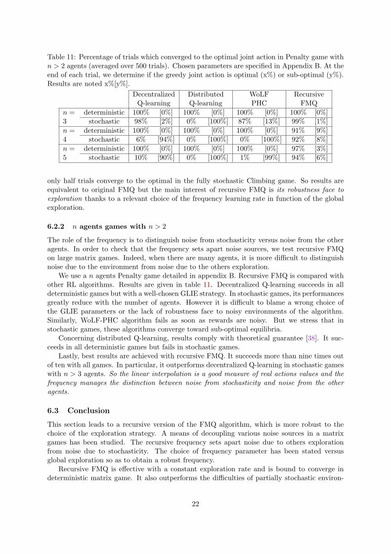
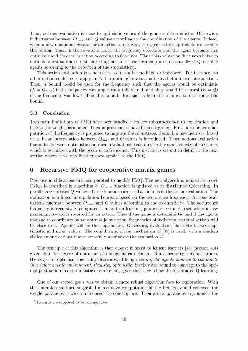
Table 11: Percentage of trials which converged to the optimal joint action in Penalty game withn > 2 agents (averaged over 500 trials). Chosen parameters are specified in Appendix B. At theend of each trial, we determine if the greedy joint action is optimal (x%) or sub-optimal (y%).Results are noted x%[y%].

Decentralized Distributed WoLF RecursiveQ-learning Q-learning PHC FMQ

n =3

deterministic 100% [0%] 100% [0%] 100% [0%] 100% [0%]stochastic 98% [2%] 0% [100%] 87% [13%] 99% [1%]

n =4


n =5


only half trials converge to the optimal in the fully stochastic Climbing game. So results areequivalent to original FMQ but the main interest of recursive FMQ is its robustness face toexploration thanks to a relevant choice of the frequency learning rate in function of the globalexploration.

6.2.2 n agents games with n > 2

The role of the frequency is to distinguish noise from stochasticity versus noise from the otheragents. In order to check that the frequency sets apart noise sources, we test recursive FMQon large matrix games. Indeed, when there are many agents, it is more difficult to distinguishnoise due to the environment from noise due to the others exploration.

We use a n agents Penalty game detailed in appendix B. Recursive FMQ is compared withother RL algorithms. Results are given in table 11. Decentralized Q-learning succeeds in alldeterministic games but with a well-chosen GLIE strategy. In stochastic games, its performancesgreatly reduce with the number of agents. However it is difficult to blame a wrong choice ofthe GLIE parameters or the lack of robustness face to noisy environments of the algorithm.Similarly, WoLF-PHC algorithm fails as soon as rewards are noisy. But we stress that instochastic games, these algorithms converge toward sub-optimal equilibria.

Concerning distributed Q-learning, results comply with theoretical guarantee [38]. It suc-ceeds in all deterministic games but fails in stochastic games.

Lastly, best results are achieved with recursive FMQ. It succeeds more than nine times outof ten with all games. In particular, it outperforms decentralized Q-learning in stochastic gameswith n > 3 agents. So the linear interpolation is a good measure of real actions values and thefrequency manages the distinction between noise from stochasticity and noise from the otheragents.

6.3 Conclusion

This section leads to a recursive version of the FMQ algorithm, which is more robust to thechoice of the exploration strategy. A means of decoupling various noise sources in a matrixgames has been studied. The recursive frequency sets apart noise due to others explorationfrom noise due to stochasticity. The choice of frequency parameter has been stated versusglobal exploration so as to obtain a robust frequency.

Recursive FMQ is effective with a constant exploration rate and is bound to converge indeterministic matrix game. It also outperforms the difficulties of partially stochastic environ-

22

Algorithm 4: Straightforward extension of recursive FMQ to Markov Games for i16


Qi(s, a)← 0, Qi,max(s, a)← 0, Fi(s, a)← 1, Ei(s, a)← 0, πi(s, a) arbitrarilys← initial statewhile s is not an absorbing state do



Qi(s, a)← (1− α)Qi(s, a) + α(r + γmaxu∈Ai

Qi(s′, u))


Qi,max(s′, u)

if q > Qi,max(s, a) thenQi,max(s, a)← q � optimistic updateFi(s, a)← 1 � occurrence frequency reset

else if q = Qi,max(s, a) thenFi(s, a)← (1− αf )Fi(s, a) + αf � recursive frequency

elseFi(s, a)← (1− αf )Fi(s, a)

Ei(s, a)← [1− Fi(s, a)]Qi(s, a) + Fi(s, a)Qi,max(s, a) � linear interpolationheuristicif Ei(s, arg max

u∈Ai


Ei(s, u) then


Ei(s, u)

∀b ∈ Ai π(s, b)←{

1 if b = amax


s← s′

end

ments. The result is an easy-to-use and robust algorithm able to solve hard repeated matrixgames. But an extension to Markov games is necessary.

7 The Swing between Optimistic or Neutral algorithm

In this section, we plan to design an algorithm for ILs in cooperative Markov games. We firstpropose a straightforward extension to Markov games of our previous recursive FMQ algorithm.But this extension presents few limits and some modifications are required to manage thecoordination. We introduce a fitting frequency for multi-state framework. The Swing betweenOptimistic or Neutral (SOoN) algorithm is then proposed. We apply the SOoN algorithm tovarious multi-state benchmarks.

7.1 Straightforward extension to Markov games

The straightforward extension of recursive FMQ to Markov Games is in algorithm 4. Thisextension is obvious except the occurrence frequency Fi(s, a) computation.

The frequency Fi(a) computed in matrix games is the probability of receiving the maximum

23

Figure 3: Two agents cooperative Markov game

reward corresponding to an action a :

Fi(a) = Pr {rt+1 = Qi,max(at)|at = a} . (17)

In Markov games, the frequency is defined as following and named myopic frequency..

Definition 13 When action a is taken at state s, the myopic frequency Fi(s, a) of agent i is theprobability that the immediate transition should return a reward and a state whose evaluation,according to a greedy policy on Qi,max, is equal to the expected maximum value of Qi,max(s, a),i.e. :

Fi(s, a) = Pr

{rt+1 + γmax

b∈Ai

Qi,max(st+1, b) = Qi,max(st, at)|st = s, at = a

}. (18)

In the straightforward FMQ extension, following functions are defined for each individualagent i :

• the value function Qi updated as in decentralized Q-learning,

• the value function Qi,max updated as in distributed Q-learning,

• the myopic frequency Fi computed according to its definition 13,

• the evaluation function Ei based on a linear interpolation between Qi and Qi,max values,

• the policy πi updated according to an equilibria selection mechanism based on a randomchoice among actions maximizing the evaluation function Ei.

The myopic frequency is an immediate measure taking only the frequency in the current stateinto account. But is this myopic frequency enough for multi-state games?

7.2 Limitations of the myopic frequency

The straightforward extension can raise issues in some cases. To explain these limitations, weperform experiments on the cooperative Markov game given in figure 3, detailed in appendix C.This benchmark is difficult because agents must coordinate in each state. Especially, we studythe development of the myopic frequency.

Optimal values of Qi,max for each agent i, at state sk, are :{Q∗

i,max(sk, a) = 10× γj−k−1

Q∗i,max(sk, b) = 10× γj−k

From the point of view of one agent, we study two cases.16Rewards are supposed to be non-negative.

24

• The agent i plays the action b at state sk, so whatever the other agent plays, the nextstate s′ is sk and for each agent i :

qi = γ maxu=1..2

Qi,max(sk, u) = 10× γj−k = Q∗i,max(sk, b) (19)

So from the viewpoint of an agent, the action b is reliable and the occurrence frequencyof receiving the Qi,max for the action b, namely Fi(sk, b), increases each time action b isplayed at s by i. Moreover, it never decreases so Fi(sk, b) converges to 1.

• The agent plays the action a at state sk. If the other agent also plays a, they coordinateand the next state s′ is sk+1 :

qi = γ maxu=1..2

Qi,max(sk+1, u) = 10× γj−k−1 = Q∗i,max(sk, a) (20)

If the other agent plays b, they mis-coordinate and the next state s′ is sk :

qi = γ maxu=1..2

Qi,max(sk, u) = 10× γj−k < Q∗i,max(sk, a) (21)

So Fi(sk, a) decreases each time the other agent plays b.

On the one hand, Fi(s, b) increases each time action b is played at state s by agent i and neverdecreases. On the other hand, Fi(s, a) decreases each time agents mis-coordinate at s. Con-sequently, from the viewpoint of one agent, the action b is safer than a. Q∗

i,max(s, a) is closeto Q∗

i,max(s, b) because Q∗i,max(s, b) = γQ∗

i,max(s, a). The evaluation E(s, b) can be higher thanE(s, a). So the exploitation strategy of the agents is to choose the joint action < b, b > and so,to remain on the spot. Its failure to coordinate is illustrated in results presented in figure 4 atpage 28 (dotted line). The number of steps per trial quickly increases since agents remain onthe spot and mis-coordinate. At the beginning of the learning, agents have a random behaviorso the number of steps per trial is low.

This example illustrates a limitation in the straightforward extension of the recursive FMQto Markov games due to the myopic frequency. This immediate measure only concerns thefrequency in the current state, which is inadequate in multi-state games. The frequency mustbe globally considered by taking frequencies of future states into account. Indeed, in a givenstate, the myopic frequency of an action could be high, but this action could lead to a statewhere the optimal action has a low myopic frequency. In other words, an action could appearinteresting in the current step according to its immediate frequency but could be a bad choiceconsidering the future.

Using a myopic frequency could mislead the algorithm. So it could be relevant to use a longterm or farsighted frequency.

7.3 Farsighted frequency

Definition 14 When action a is played at state s, the farsighted frequency Gi(s, a) for agenti is the probability that all future transitions return rewards and states whose evaluations, ac-cording to a greedy policy on Qi,max, are equal to the expected maximum value Qi,max for thesestates, i.e. :

Gi(s, a) = P πmaxr

{rt+1 + γmax

b∈Ai

Qi,max(st+1, b) = Qi,max(st, at) ∧

rt+2 + γmaxb∈Ai

Qi,max(st+2, b) = Qi,max(st+1, at+1) ∧ . . . |st = s, at = a

}(22)

25

The question is how to estimate this farsighted frequency?

We make the assumption that precedent events are independent, i.e. the occurrence of oneevent makes it neither more nor less probable that the other occurs. So the statement above isequivalent to :

Gi(s, a) = P πmaxr

{rt+1 + γmax

b∈Ai

Qi,max(st+1, b) = Qi,max(st, at)|st = s, at = a

}×

P πmaxr

{rt+2 + γmax

b∈Ai


}. (23)

According to the definition 13, the first term of the previous equation is equal to Fi(s, a). Andthanks to the total probability theorem, the second term is :

P πmaxr

{rt+2 + γmax

b∈Ai


}=

∑s′∈S

P πmaxr

{rt+2 + γmax

b∈Ai

Qi,max(st+2, b) = Qi,max(st+1, at+1) ∧ . . . |st = s, at = a, st+1 = s′}×

Pr

{st+1 = s′|st = s, at = a

}. (24)

The πmax policy is following so at+1 ∈ arg maxb∈Ai

Qi,max(st+1, b) and :

Gi(s, a) = Fi(s, a)∑s′∈S

Pr

{st+1 = s′|st = s, at = a

}Gi(s′, arg max

b∈Ai

Qi,max(st+1, b)) (25)

If P ass′ is the probability of each next possible state s′ given a state s and an action a, we obtain :

Gi(s, a) = Fi(s, a)∑s′∈S

P ass′Gi(s′, arg max

u∈Ai

Qi,max(s′, u)) (26)

As P ass′ is unknown, we suggest to evaluate the farsighted frequency by following a temporal

difference recursive computation :

Gi(s, a)← (1− αg)Gi(s, a) + αgFi(s, a) maxv∈arg max

u∈Ai

Qi,max(s′,u)Gi(s′, v) (27)

where αg ∈ [0; 1] is the learning rate of the farsighted frequency. The improvement suppliedto the farsighted frequency is the product of the current state-action couple myopic frequencywith the myopic frequency of the optimal action in the next state. Thus, if an action has atcurrent state a high myopic frequency, but can lead to a state where the optimal action has alow farsighted frequency, then, this action will have a low farsighted frequency.

We could draw connections between the farsighted frequency general idea and bonus prop-agation for exploration [46]. Bonus propagation leads to a full exploration of the environmentthanks to a mechanism of retro-propagation concerning local measures of exploration bonuses.In the case of the farsighted frequency, values of myopic frequencies are spread : for each vis-ited state, the agent “looks forward” future states to take into account values of frequencies ofoptimal actions in these states.

26

Algorithm 5: SOoN algorithm for Markov Game for agent i17


Qi(s, a)← 0, Qi,max(s, a)← 0, Fi(s, a)← 1, Gi(s, a)← 1, Ei(s, a)← 0, πi(s, a)arbitrarily

s← initial statewhile s is not an absorbing state do



Qi(s, a)← (1− α)Qi(s, a) + α(r + γmaxu∈Ai

Qi(s′, u))


Qi,max(s′, u)

if q > Qi,max(s, a) thenQi,max(s, a)← q � optimistic updateFi(s, a)← 1 � myopic frequency resetGi(s, a)← 1 � farsighted frequency reset

else if q = Qi,max(s, a) thenFi(s, a)← (1− αf )Fi(s, a) + αf � frecursive myopic frequency

elseFi(s, a)← (1− αf )Fi(s, a)

� farsighted frequency updateGi(s, a)← (1− αg)Gi(s, a) + αgFi(s, a) max

v∈arg maxu∈Ai

Qi,max(s′,u)Gi(s′, v)

� linear interpolation heuristicEi(s, a)← [1−Gi(s, a)]Qi(s, a) +Gi(s, a)Qi,max(s, a)if Ei(s, arg max

u∈Ai


Ei(s, u) then


Ei(s, u)

∀b ∈ Ai πi(s, b)←{

1 if b = amax


s← s′

end

7.4 Swing between Optimistic or Neutral algorithm

We use the farsighted frequency in a new algorithm, named Swing between Optimistic or Neu-tral (SOoN) and detailed in algorithm 5. Same functions as those defined at §7.1 are used. Thenovelty is the state-action evaluation based on the farsighted frequency G. The evaluation of astate-action couple sways from distributed Qmax values to decentralized Q values according toG values and so according to a detection of stochasticity in the game. In deterministic Markovgames, the farsighted frequency tends toward 1 and thus, the SOoN algorithm is close to thedistributed Q-learning and is insured to converge towards optimal joint actions. Otherwise, instochastic Markov games, the farsighted frequency is between 0 and 1 and the SOoN algorithmswings between optimistic or neutral evaluations.

We apply the SOoN algorithm to the cooperative Markov game of the figure 3 where thecoordination of the two agents is difficult. Results are given in figure 4 (solid line). It is obvious

27

0 20 40 60 80 100 120 140 160 180 2000

100

200

300

400

500

600

Ste

ps t

o g

oa

l

Trial number

Straightforward extension of recursive FMQSOoN algorithm

Figure 4: Two agents cooperative Markov game experiments with 10 states averaged over 200runs (α = 0.1, γ = 0.9, αf = 0.05, αg = 0.3, ε = 0.05). Steps to goal vs. trial number.

Figure 5: Boutilier’s coordination game.

that the agents then manage the coordination after 15 trials thanks to the use of the farsightedfrequency.

7.5 Experimentations on Markov game benchmarks

We now show results of applying the SOoN algorithm to a number of different Markov games.We compare the performance of decentralized Q-learning, distributed Q-learning, WoLF-PHC,hysteretic Q-learning and SOoN. The domains include various levels of difficulty according to theagents number (2 and more), the state observability (full or incomplete), and mis-coordinationfactors (shadowed equilibria, equilibria selection, deterministic or stochastic environments). Foreach benchmarks, we state what is at stake in the learning of ILs. Moreover, and in a concernto be fair, all algorithms used ε-greedy selection method with a stationary strategy and globalexploration of ψ = 0.1. It allows to check the robustness face to the exploration of each method.

7.5.1 Boutilier’s coordination Markov games

The Boutilier’s coordination game with two agents was introduced in [47] and is shown infigure 5. This multi-state benchmark is interesting because all mis-coordination factors can

17Rewards are supposed to be non-negative.

28

Table 12: Percentage of cycles which converged to the optimal joint action (averaged over 50cycles). We set α = 0.1, γ = 0.9, δlose = 0.006, δwin = 0.003, αf = 0.01, αg = 0.03, ε = 0.05.β = 0.01 in deterministic games and β = 0.05 in stochastic games. At the end of each cycle, wedetermine if the greedy joint action is optimal.

Boutilier’s coordination gamedeterministic stochastic

k = 0 k = −100 k = 0 k = −100Decentralized Q-learning 100% 6% 100% 12%Distributed Q-learning 100% 100% 0% 0%

WoLF-PHC 100% 36% 100% 40%Hysteretic Q-learning 100% 100% 100% 30%

SOoN 100% 100% 100% 96%

easily be integrated and combined. At each state, each agent has a choice of two actions. Thetransitions on the diagram are marked by a pair of corresponding actions, denoting player 1’smove and player 2’s move respectively. “ * ” is a wild card representing any action. Statesthat yield a reward are marked with the respective value. All other states yield a reward of 0.A coordination issue applies in the second state of the game. Both agents should then agreeon the same action. Moreover, there are two optimal equilibria so the agents are face to anequilibria selection problems and must coordinate on the same. Mis-coordination in the secondstate produces a penalty k. So the potential of choosing the action a for the first agent inthe state s1 is shadowed by the penalty k associated to mis-coordination. We also propose apartially stochastic version of the Boutilier’s game with a random reward (14 or 0) received instate s6 with equal probability instead of 7.

A trials ends when agents reach one of the absorbing states (s4, s5 or s6). One cycle consistsof 50000 learning trials. At the end of each cycle, we determine if the greedy joint action isoptimal. Results are in table 12.

In deterministic game with k = 0, all algorithms manage the coordination. Similarly,in the stochastic game with k = 0, all algorithms except for distributed Q-learning succeed.Indeed, an easy way to put Distributed Q-learning agents in the wrong is to insert stochasticrewards. So distributed Q-learning never manages the coordination in the partially stochasticBoutilier’s game. When mis-coordination penalties are introduced in the deterministic game,decentralized Q-learning and WoLF-PHC fail because of shadowed equilibria. Distributed Q-learning, hysteretic Q-learning and SOoN succeed in the coordination. But in the stochasticversion with k = −100, SOoN is the only one to be close to 100% of optimal joint action.

So SOoN gets best convergence results. In deterministic games, it turns towards the Dis-tributed Q-learning. In the stochastic Boutilier’s game without penalties, it turns towards thedecentralized Q-learning. In the stochastic game with penalties, SOoN outperforms all otheralgorithms. The linear interpolation to evaluate state-action couples is a pertinent heuristic tomeasure real values of actions.

7.5.2 Two predators pursuit domains

The pursuit problem is a popular multi-agent domain in which some agents, called predators,have to capture one or several preys in a gridworld [48]. In the two agents pursuit domains,predators have to explicitly coordinate their actions in order to capture a single prey in adiscrete 10× 10 toroidal grid environment (Fig. 6a). At the beginning of each trial, predatorsand prey are set up in distinct random positions. At each time step, all predators simultaneously

29

(a) Complete 10 × 10 toroidal grid. (b) Possible captureposition.

Figure 6: Two predators pursuit problem.

execute one of the 5 possible actions : move north, south, east, west or stand still. Moreover,noise is added to the environment through uncertainty in actions results. Any action movesa predator in the intended direction with probability 0.8, and otherwise a random action isapplied. The prey moves according to a randomized policy : it remains on its current positionwith a probability of 0.2, and otherwise moves to ones of its free adjacent cells with uniformprobability. A prey is captured when both predators are located in cells adjacent to the prey,and one of the two predators moves to the location of the prey while the other predator remains,for support, on its current position (Fig. 6b). A trials ends when the prey is captured.

The state space is represented by the relative position of the two predators to the prey. Soeach IL computes a Qi table with 99× 98× 5 values, i.e. 48510 different state-action pairs foreach of both agents. A capture results in a reward R = 10 for every agent, and predators andprey are replaced to distinct random positions. Furthermore, predators receive penalties in caseof mis-coordination. They both receive a penalty of −50 when one of them moves to the preywithout support or when they end up in the same cell. Then both are moved to a random,empty cell. In all other situations, the reward is 0.

The main factors which complicate the coordination are action shadowing induced by penal-ties and the stochastic environment due to the random behavior of the prey and the uncertaintyin actions results.

A trial consists of 10000 steps. We make out learning trials and greedy trials in which agentsare following their learned greedy policies. After each learning trial is done a greedy trial. Foreach greedy trial, we plot the number of captures per trial and the sum of received rewards peragent during the trial. With the number of captures per trial, we can compare greedy policieslearned with each algorithm; with the sum of received rewards, the number of collisions ornon-support is observed. Results obtained on 10000 greedy trials are given in figure 7. We cannotice that :

• greedy policies learned by decentralized Q-learning fail to coordinate,

• there is the same number of capture with WoLF-PHC and hysteretic Q-learning, but thesecond one creates less collisions,

• despite the stochastic environment, greedy policies learned by distributed Q-learning man-age the coordination with around 45 captures per trial. However, collisions are not much

30

avoided,

• SOoN gets best results. After around 4500 trials, it outperforms distributed Q-learning.Two phases can be identified : during a first phase, SOoN behaves as distributed Q-learning (2000 first trials). Indeed, agents are initially optimistic. This first stage is insome way an adaptative phase to the environment; the frequency refines according to thestochasticity of the environment. Then evaluations swing between optimistic or neutral.The second phase is when SOoN manages the coordination : the number of capturesincreases and overcome all other results. So SOoN realizes an automatic adaptation to theenvironment.

7.5.3 Four agents pursuit domains

In the four agents pursuit domains, four predators have to coordinate their actions in order tosurround a single prey in a discrete 7×7 toroidal grid environment (Fig. 8a). Agents observationssuffer from low resolution. Indeed, a predator perceives the others according to the 8 cardinaldirections and a close or distant criterion (Fig. 8b), so 16 perceptions. Given that each predatorperceives its 3 teammates plus the prey, there are 164 possible observations per agent. Eachagent has 5 possible actions, i.e. a Qi-table of size 164 × 5 for each predator. Concerning thereinforcement function, if at least one agent is in the situation in figure 8c, every agent receivesR = 25. When the prey is captured, they each receive R = 100. The low resolution in theperception induces stochasticity in the environment so the main factor here which complicatesthe coordination of predators is the noise.

A trial consists of 1000 steps. We make out learning trials and greedy trials in which agentsare following their learned greedy policies. After each learning trial is done a greedy trial. Foreach greedy trial, we plot the number of captures per trial (Fig. 9). We can compare greedypolicies learned with each algorithm. We can notice that :

• it is very difficult for distributed Q-learning to do the coordination. Indeed, optimisticagents capture the prey for the first time after 48000 trials, and they capture the prey 5times per trial at 80000 trials. The low resolution in perceptions induces stochasticity inthe environment which puts optimistic agents in the wrong,

• decentralized Q-learning shows interesting results in this stochastic environment. It con-firms that this algorithm can be applied with success on some MAS and manages thecoordination,

• WoLF-PHC is the first one to achieve captures but its performance increases slowly,

• hysteretic Q-learning manages first captures late, but its performance increases fast. Itnotably overcomes WoLF-PHC and is close to decentralized Q-learning after 80000 trialswith around 60 captures per trial,

• SOoN gets best results. Two phases can be identified. During the first adaptative phase,agents are initially optimistic so SOoN does not manage any captures as distributed Q-learning. Then, once the frequency is fitted to the environment, the number of capturesper trial increases. It is the second phase of coordination. After around 50000 trials, 90captures are managed per trial. SOoN realizes an automatic adaptation to the environ-ment.

We can also notice that greedy policies learned with SOoN and decentralized Q-learning arenoised, unlike WoLF-PHC or distributed Q-learning policies. So even if SOoN realizes a fastand successful coordination, it is more sensitive to the stochasticity in this game.

31

7.5.4 Discrete smart surface with 270 agents

Given our real world application of a decentralized control of a smart surface, we have developeda discrete smart surface benchmark. The system is composed of 270 actuators organized in array(Fig. 10). At each time step, all actuators simultaneously execute one of the 5 possible actions :up, down, right, left or nop, represented by arrows and a circle. Uncertainty is added to actionsresults : with a probability 0.001, each actuator executes a random action. An object is situatedon the surface. The motion of the object is proportional to the actions sum of the actuatorswhich are under and by the object. The influence factor on the actions of the actuators by theobject is three times higher than the influence factor on the actions of the actuators under theobject. The object moves in the four cardinal directions but it does not rotate. Additionally,the object cannot get out of the surface and instead stays by the edge. The system’s state isthe index position of the object (according to its up and left corner). Each actuator is drivenby an independent agent so it has only access to the index position and to its action. In realapplication, the full state observability can be done thanks to an overhead camera that extractsthe index position.

The goal is for the agents to cooperate so as to move the object to a goal position. Then,all agents receive R = 10 and the trial ends. If the object is getting closer to the vertical edgesof the surface, every agent receives a penalty (R = −50). Otherwise, the reward is 0.

A trial starts with the object at its initial position and ends when the object reaches thegoal position (absorbing state). For each trial, we plot the number of steps to the goal and thesum of received rewards per agent (Fig. 11). With the sum of received rewards, we can observeif the object is getting closer to the vertical edges of the surface. With the number of steps tothe goal, we can check if the learned policies are close to best policy achieved “by hand”‘ whichmakes 3 steps per trial (without uncertainty). We can notice that :

• the environment is stochastic so distributed Q-learning fails to coordinate. Moreover,optimistic agents are unaware of penalties so they do not avoid edges of the surface; thesum of received rewards per trial is low,

• decentralized Q-learning shows interesting results : after 300 trials, 20 steps are requiredto reach the goal and the object is getting closer to the vertical edges around 4 timesper trial. However, learned policies are not stable. Mis-coordination penalties and thelack of robustness face to exploration lead to destruction of individual policies. Duringthe experimentations, we notice that agents coordinate to avoid edges : the object moveround in circles in the area without penalties,

• hysteretic Q-learning is close to decentralized Q-learning. But as these agents are chieflyoptimistic, they do not avoid as much the edges and the sum of rewards increases slowly,

• with WoLF-PHC, learned policies are stable but slow,

• after 300 trials, best results are obtained with SOoN : 12 steps are required to reach thegoal and the object is getting closer to the vertical edges around once per trial. Moreover,these performances are achieved from 100 trials. Again two phases draw attention. Thefirst phase of adaptation when agents are initially optimistic and so fails to move theobject to the goal. Then, SOoN adapts its frequency to the environment : the number ofsteps to goal decreases. So the second phase is the coordination.

32

7.6 Conclusion

In this section, the objective was to design an algorithm for ILs, robust face to explorationand mis-coordination factors in cooperative Markov games. Starting from the recursive FMQ,we show that using a one-step lookahead with the myopic frequency in multi-stage gamescould mislead the algorithm. So we introduced the computation of a farsighted frequencyto detect the stochasticity of the game. This frequency is used in a heuristic to evaluatestate-action couples in the Swing between Optimistic or Neutral algorithm. This heuristic isbased on a linear interpolation between optimistic or neutral evaluations. Thus, SOoN realizesan automatic adaptation to the environment stochasticity of its evaluations. Especially, twophases are characteristic of this method. An adaptative phase when the frequency detects thestochasticity. Indeed, at the beginning, agents are optimistic. If the environment is deterministicand the agents manage the coordination, agents stay optimistic. Otherwise, the frequencyadjusts evaluations between optimistic or neutral. When these evaluations are adjusted, thesecond phase is the successful coordination of agents. These both phases have been illustratedwith some experimentations on Markov games. They confirm that the linear interpolation is apertinent evaluation of real values of state-actions. They also highlight that SOoN is able toovercome mis-coordination factors and is robust face to exploration.

8 Conclusion

In this report, we focused on the learning of independent agents in cooperative multi-agentsystems. First, we highlighted some of the difficulties encountered by ILs in this framework.Especially, we analyzed some factors which complicate the ILs coordination : shadowed equi-libria, equilibria selection and noise. These factors have been identified and interpreted inmatrix games. The impact of the exploration has also been studied as a major stake in thereinforcement learning of ILs.

Through a section suggesting a uniform notation, related algorithms based on Q-learninghave been reviewed according to some factors : the robustness face to exploration, the learningof optimal individual policies despite shadowed equilibria and noise, and the selection of a singleoptimal equilibria. Thanks to this study, we focused on developing an algorithm robust face tothe exploration strategy and able to overcome mis-coordination factors in cooperative Markovgames. For that, we emphasized common points between FMQ heuristic and distributed Q-learning. On the one hand, distributed Q-learning is robust face to exploration and insured toconverge toward a Pareto optimal Nash equilibrium in deterministic Markov games. On theother hand, FMQ outperforms the difficulty of weakly noisy matrix games by decoupling noisedue to agents behaviors and noise due to the environment.

Thus, we contribute to improve the FMQ algorithm in matrix games and propose a recursiveversion which is easy-to-use, robust and able to solve hard repeated matrix games. We furtherproposer the SOoN algorithm, standing for “Swing between Optimistic or Neutral”. Thanksto the computation of a farsighted frequency and to a novel evaluation of the state-actionvalues, this algorithm sways automatically from optimistic to neutral evaluation according to adetection of the noise in the environment. At the beginning, the environment is supposed to bedeterministic and so agents are optimistic. Then, the SOoN automatically adapts its frequencyto the stochasticity of the environment through the assessment of the probability of attainingthe optimal gain.

We specify the choice of the two parameters of the SOoN so as to obtain an algorithm robustface to the exploration. The noise due to agents behaviors has been defined with the globalexploration. We demonstrate empirically the robustness and advantages of the SOoN algorithm

33

Table 13: Characteristics of RL algorithms for independent learners in cooperative games.Entries marked with “NT” indicate it has not been tested.

Mat

rix

Gam

es

Mar

kov

Gam

esE

quili

bria

Sele

ctio

n

Shad

owed

Equ

ilibr

ia

Stoc

hast

ic

envi

ronm

ent

Rob

ust

face

toex

plor

atio

n

Decentralized � � � � lowQ-Learning [31] with GLIE partially

Distributed � � � � totalQ-Learning [38]

Lenient learners [43] � NT NT NT lowHysteretic � � � � � low

Q-Learning [42] with GLIE partiallyWoLF PHC [39] � � � NT good

FMQ [29] � � � � lowwith GLIE partially

Recursive FMQ � � � � goodpartially

SOoN � � � � � goodpartially

on a number of multiple states cooperative Markov games with numerous agents. Results showthat this algorithm overcomes all mis-coordination factors, even weakly noise Markov games,and is robust face to the exploration strategy (table 13). The SOoN manages the coordinationthanks to two characteristic phases : an adaptative phase where the frequency automaticallyfits to the stochasticity, and the coordination phase where the agents coordinate themselves.Moreover, results confirm that the linear interpolation can be a pertinent evaluation of realvalues of state-action couples, especially in stochastic games.

Our research has raised a number of issues to be investigated in on-going and future work.The first perspective is to test the SOoN algorithm on a real problem as the decentralizedcontrol of a smart surface.

The second perspective is to improve the proposed evaluation of action. Indeed, we presentedencouraging experimental results, but the proposed linear interpolation to evaluate a state-action couple could be modified. Specifically, a bound for the farsighted frequency could bedefined to mark optimistic or neutral evaluation out.

An other prospect concerns a common issue in RL of making algorithms scale to large prob-lems. Indeed, the SOoN algorithm uses explicit table representations of Q, Qmax and frequencyfunctions. In larger state-action spaces application scenarios, explicit table representations be-come intractable. So it would be interesting to generalize and approximate these tables withsome kind of function approximation mechanism. So an interesting direction of this work is tocombine function approximation mechanism with the SOoN algorithm.

34

Appendix A :

The following were the learning and decay rates used for the results presented in §4. Here t isthe number of repetitions of the game. With the detailed algorithmic descriptions in section 4and these parameters details, all of the presented results are reproducible.

• Decentralized Q-learning

α = 0.1 γ = 0 τ = 5000× 0.997t

• Distributed Q-learningα = 1 γ = 0 ε = 0.05

• Hysteretic Q-learning

α = 0.1 β = 0.01 γ = 0 τ = 5000e−0.003t

• Original FMQα = 0.1 γ = 0 c = 10 τ = 499e−0.006t + 1

Appendix B :

In the Penalty game with n > 2 agents, each agent has 3 actions a, b and c. If half agents ormore play a and the others play c, the received reward is 10. If less than half agents play a andthe others play c, the received reward is −100 since they fail to coordinate. If half agents ormore play b and the others play c, the received reward is 2. Otherwise, the reward is 0.

There are many Pareto optimal Nash equilibria when half agents or more play a and theothers play c. These optimal equilibria are shadowed by penalties in case of mis-coordination.There are also many sub-optimal Nash equilibria when half agents or more play b and the othersplay c. So this game presents mis-coordination factors. Additionally, the reward can be noised :instead of receiving a reward equal to 2, 12 and 6 are received with equal probabilities.

The following were the learning and decay rates used for the results presented in §6.2. Heret is the number of repetitions of the game. With the detailed algorithmic descriptions and theseparameters details, all of the presented results are reproducible.

• decentralized Q-learning

Table 14: Learning parameters choices with decentralized Q-learning.agents repetitions algorithm decision explorationnumber per trial parameters method strategyn = 3 t = 30000 α = 0.1 softmax GLIE

γ = 0 τ(t) = 5000 ∗ exp(−0.0003 ∗ t)n = 4 t = 50000 α = 0.1 softmax GLIE

γ = 0 τ(t) = 5000 ∗ exp(−0.0002 ∗ t)n = 5 t = 80000 α = 0.1 softmax GLIE

γ = 0 τ(t) = 5000 ∗ exp(−0.0001 ∗ t)

• recursive FMQ

• WoLF-PHC

35

Table 15: Learning parameters choices with recursive FMQ.agents repetitions algorithm decision explorationnumber per trial parameters method strategyn = 3 t = 30000 α = 0.1 αf = 0.01 ε-greedy stationary

γ = 0 Qmax,ini = −100 ψ = 0.1n = 4 t = 50000 α = 0.1 αf = 0.001 ε-greedy stationary

γ = 0 Qmax,ini = −100 ψ = 0.15n = 5 t = 80000 α = 0.1 αf = 0.0001 ε-greedy stationary

γ = 0 Qmax,ini = −100 ψ = 0.2

Table 16: Learning parameters choices with WoLF-PHC.agents repetitions algorithm decision explorationnumber per trial parameters method strategyn = 3 t = 30000 α = 0.1 δlose = 0.006 ε-greedy stationary

γ = 0 δwin = 0.001 ψ = 0.1n = 4 t = 50000 α = 0.1 δlose = 0.0006 ε-greedy stationary

γ = 0 δwin = 0.0001 ψ = 0.15n = 5 t = 80000 α = 0.1 δlose = 0.0006 ε-greedy stationary

γ = 0 δwin = 0.0001 ψ = 0.2

Appendix C :

The following is the description of the cooperative Markov game in figure 3. Each agent hasa choice of two actions a and b. The game starts in state s1. The transitions on the figureare marked by a pair of corresponding actions, denoting agent 1’s action and agent 2’s actionrespectively. “ * ” is a wild card representing any action. So if both agents are coordinatedon the joint action < a, a > in the state sk, they move to the next state sk+1. If at least oneagent plays b, they remain on the spot. When agents reach the absorbing state sj , they receivea reward 10. All other states yield a reward of 0.

References

[1] Lucian Busoniu, Robert Babuska, and Bart De Schutter. Multi-agent reinforcement learn-ing: A survey. In Int. Conf. Control, Automation, Robotics and Vision, pages 527–532,December 2006. 1

[2] Peter Stone and Manuela M. Veloso. Multiagent systems: A survey from a machine learningperspective. Autonomous Robots, 8(3):345–383, 2000. 1

[3] R. S. Sutton and A. G. Barto. Reinforcement Learning: An Introduction. The MIT Press,Cambridge, 1998. 1, 3

[4] Erfu Yang and Dongbing Gu. Multiagent reinforcement learning for multi-robot systems:A survey. Technical report, Department of Computer Science, University of Essex, 2004. 1

[5] C.H. Papadimitriou and J.N. Tsitsiklis. On the complexity of designing distributed proto-cols. Information and Control, 24(4):639–654, 1982. 1

36

[6] C.H. Papadimitriou and J.N. Tsitsiklis. The complexity of markov decision processes.Mathematics of Operations Research, 12(3):441–450, 1987. 1

[7] D. Bernstein, R. Givan, N. Immerman, and S. Zilberstein. The complexity of decentralizedcontrol of markov decision processes. Math. Oper. Res., 27(4):819–840, 2002. 1

[8] Nancy Fulda and Dan Ventura. Predicting and preventing coordination problems in cooper-ative q-learning systems. In Proceedings of the International Joint Conference on ArtificialIntelligence, 2007. 1, 6

[9] Gang Chen, Zhonghua Yang, Hao Ge, and Kiah Mok Goh. Coordinating multiple agentsvia reinforcement learning. Autonomous Agents and Multi-Agent Systems, 10(3):273–328,2005. 1

[10] Andrew Garland and Richard Alterman. Autonomous agents that learn to better coordi-nate. Autonomous Agents and Multi-Agent Systems, 8(3):267–301, 2004. 1

[11] Robert H. Crites and Andrew G. Barto. Elevator group control using multiple reinforcementlearning agents. Machine Learning, 33(2-3):235–262, 1998. 1

[12] Katja Verbeeck, Ann Nowe, Johan Parent, and Karl Tuyls. Exploring selfish reinforcementlearning in repeated games with stochastic rewards. Autonomous Agents and Multi-AgentSystems, 14(3):239–269, 2007. 1

[13] Kagan Tumer and Adrian Agogino. Distributed agent-based air traffic flow management. InAAMAS ’07: Proceedings of the 6th international joint conference on Autonomous agentsand multiagent systems, pages 1–8, New York, NY, USA, 2007. ACM. 1

[14] D.H. Wolpert, J. Sill, and K. Tumer. Reinforcement learning in distributed domains:Beyond team games. In Proceedings of the Seventeenth IJCAI, 2001. 1

[15] Y. Fukuta, Y.A. Chapuis, Y. Mita, and H. Fujita. Design, fabrication and control of mems-based actuator arrays for air-flow distributed micromanipulation. J. Microelectromech.Syst., 15(4):912 – 926, 2006. 1

[16] Y. Uny Cao, Alex S. Fukunaga, and Andrew B. Kahng. Cooperative mobile robotics:Antecedents and directions. Autonomous Robots, 4(1):7–23, March 1997. 1

[17] M. Tan. Multiagent reinforcement learning: Independent vs. cooperative agents. In 10thInternational Conference on Machine Learning, pages 330–337, 1993. 2, 10

[18] Richard Bellman. Dynamic Programming. Princeton University Press, Princeton, NJ, 1957.2

[19] Richard Bellman. A markov decision process. Journal of Mathematical Mechanics, 6:679–684, 1957. 2

[20] M. L. Puterman. Markov Decision Processes: Discrete Stochastic Dynamic Programming.John Wiley and Sons, 1994. 3

[21] L. P. Kaelbling, Michael Littman, and Andrew Moore. Reinforcement learning: A survey.Journal of Artificial Intelligence Research, 4:237–285, 1996. 3

[22] John Von Neumann and Oskar Morgenstern. Theory of Games and Economic Behavior.Princeton University Press, 1944. 3

37

[23] M. J. Osborne and A. Rubinstein. A course in game theory. MIT Press, 1994. 3, 4

[24] John F. Nash. Equilibrium points in n-person games. In Proceedings of the NationalAcademy of Sciences of the United States of America, volume 36, pages 48–49, 1950. 4

[25] L.S. Shapley. Stochastic games. Proc. Nat. Acad. Sci. USA, 39:1095–1100, 1953. 5

[26] Leonid Peshkin, Kee-Eung Kim, Nicolas Meuleau, and Leslie P. Kaelbling. Learning to co-operate via policy search. In Sixteenth Conference on Uncertainty in Artificial Intelligence,pages 307–314, San Francisco, CA, 2000. Morgan Kaufmann. 5

[27] N. Vlassis. A concise introduction to multiagent systems and distributed AI. InformaticsInstitute, University of Amsterdam, 2003. 6

[28] Caroline Claus and Craig Boutilier. The dynamics of reinforcement learning in coopera-tive multiagent systems. In Proceedings of the Fifteenth National Conference on ArtificialIntelligence, pages 746–752, 1998. 7, 10

[29] S. Kapetanakis and D. Kudenko. Reinforcement learning of coordination in cooperativemulti-agent systems. In Proceedings of the Nineteenth NCAI, 2002. 7, 12, 15, 18, 34

[30] Craig Boutilier. Planning, learning and coordination in multiagent decision processes. InTheoretical Aspects of Rationality and Knowledge, pages 195–201, 1996. 8, 11

[31] C.J.C.H. Watkins and P. Dayan. Technical note: Q-learning. Machine Learning, 8:279–292,1992. 9, 10, 15, 34

[32] Lucian Busoniu, Robert Babuska, and Bart De Schutter. Decentralized reinforcement learn-ing control of a robotic manipulator. In Proceedings of the 9th International Conference onControl, Automation, Robotics and Vision (ICARCV 2006), pages 1347–1352, Singapore,December 2006. 10

[33] Sandip Sen and Mahendra Sekaran. Individual learning of coordination knowledge. JETAI,10(3):333–356, 1998. 10

[34] Sandip Sen, Mahendra Sekaran, and John Hale. Learning to coordinate without sharinginformation. In Proceedings of the Twelfth National Conference on Artificial Intelligence,pages 426–431, Seattle, WA, 1994. 10

[35] Y. Wang and C. W. de Silva. Multi-robot box-pushing: Single-agent q-learning vs. teamq-learning. In Proc. of IROS, pages 3694–3699, 2006. 10

[36] Satinder P. Singh, Tommi Jaakkola, Michael L. Littman, and Csaba Szepesvari. Conver-gence results for single-step on-policy reinforcement-learning algorithms. Machine Learn-ing, 38(3):287–308, 2000. 10

[37] S. Kapetanakis and D. Kudenko. Improving on the reinforcement learning of coordinationin cooperative multi-agent systems. Second Symposium on Adaptive Agents and Multi-Agent Systems(AISB/AAMAS-II), Imperial College, London, April 2002. 10

[38] M. Lauer and M. Riedmiller. An algorithm for distributed reinforcement learning in co-operative multi-agent systems. In Proc. 17th International Conf. on Machine Learning,pages 535–542. Morgan Kaufmann, San Francisco, CA, 2000. 11, 15, 18, 19, 22, 34

38

[39] Michael Bowling and Manuela Veloso. Multiagent learning using a variable learning rate.Artificial Intelligence, 136:215–250, 2002. 11, 15, 34

[40] Bikramjit Banerjee and Jing Peng. Adaptive policy gradient in multiagent learning. InAAMAS ’03: Proceedings of the second international joint conference on Autonomousagents and multiagent systems, pages 686–692, New York, NY, USA, 2003. ACM. 11

[41] M. Bowling. Convergence and no-regret in multiagent learning. In Y. Weiss L. K. Saul andL. Bottou, editors, Advances in Neural Information Processing Systems, pages 209–216.MIT Press, 2005. 11

[42] Laetitia Matignon, GuillaumeJ. Laurent, and Nadine Le Fort-Piat. Hysteretic q-learning:an algorithm for decentralized reinforcement learning in cooperative multi-agent teams.In Proceedings of IEEE/RSJ International Conference on Intelligent Robots and SystemsIROS 2007, pages 64–69, San Diego, CA, USA, Nov. 2007. 11, 15, 34

[43] Liviu Panait, Keith Sullivan, and Sean Luke. Lenient learners in cooperative multia-gent systems. In AAMAS ’06: Proceedings of the fifth international joint conference onAutonomous agents and multiagent systems, pages 801–803, New York, NY, USA, 2006.ACM Press. 12, 15, 19, 34

[44] Keith Sullivan, Liviu Panait, Gabriel Balan, and Sean Luke. Can good learners alwayscompensate for poor learners? In AAMAS ’06: Proceedings of the fifth international jointconference on Autonomous agents and multiagent systems, pages 804–806, New York, NY,USA, 2006. ACM Press. 12

[45] Spiros Kapetanakis and Daniel Kudenko. Reinforcement learning of coordination in hetero-geneous cooperative multi-agent systems. In AAMAS ’04: Proceedings of the Third Interna-tional Joint Conference on Autonomous Agents and Multiagent Systems, pages 1258–1259,Washington, DC, USA, 2004. IEEE Computer Society. 12

[46] Nicolas Meuleau and Paul Bourgine. Exploration of multi-state environments: Local mea-sures and back-propagation of uncertainty. Machine Learning, 35(2):117–154, 1999. 26

[47] Craig Boutilier. Sequential optimality and coordination in multiagent systems. In IJCAI,pages 478–485, 1999. 28

[48] M. Benda, V. Jagannathan, and R. Dodhiawala. On optimal cooperation of knowledgesources - an experimental investigation. Technical Report BCS-G2010-280, Boeing Ad-vanced Technology Center, Boeing Computing Services, Seattle,Washington, 1986. 29

39

0 1000 2000 3000 4000 5000 6000 7000 8000 9000 100000

10

20

30

40

50

60

Trial number

Num

ber o

f cap

ture

s pe

r tria

ldecentralized Q−learningdistributed Q−learningWoLF PHChysteretic Q−learningSOoN

(a)

0 1000 2000 3000 4000 5000 6000 7000 8000 9000 10000−1000

−800

−600

−400

−200

0

200

400

Trial number

Sum

of r

ecei

ved

rew

ards

per

tria

l

decentralized Q−learningdistributed Q−learningWoLF PHChysteretic Q−learningSOoN

(b)

Figure 7: Number of captures and sum of received rewards per agent for 10000 steps (averagedover 20 runs) with α = 0.1, β = 0.01, αf = 0.01, αg = 0.3, δlose = 0.06, δwin = 0.03, γ = 0.9.

40

(a) Capture (b) Perceptions (c) Reinforcement

Figure 8: Four predators pursuit problem. a) The prey is captured. b) (2 × 8)4 perceptionsper agent. c) The reinforcement is attributed in an individual way and is only function of localperceptions (and similar situations obtained by rotation of 90◦).

� � � � � � � � ��

�

��

��

��

��

��

��

��

�

��

��

� ��

��

��

�� !�� !"�#$ %&'()�� !*+��

Figure 9: Number of captures for 80000 steps (averaged over 5 runs) with α = 0.3, β = 0.03,αf = 0.03, αg = 0.3, δlose = 0.06, δwin = 0.03, γ = 0.9.

41

Figure 10: Discrete smart surfacebenchmark with 9× 30 agents.

� ��

��

��

��

��

� �

��

�� !"#$�� %&��

� ��

��

��

��

��

��

��

��

��

�� !�"#$%&�� '�(

Figure 11: Steps to goal (on the top) and sum of rewardsreceived at each trial by an agent (on the bottom) vs. trialnumber (averaged over 100 runs and logarithmic scale).α = 0.1, αf = 0.01, αg = 0.3, γ = 0.9 and ε = 0.0005.

42

coordination of independent learners in cooperative markov

Documents