FINITE HORIZON MARKOV DECISION PROBLEMS

AND A CENTRAL LIMIT THEOREM FOR TOTAL REWARD

ALESSANDRO ARLOTTO AND J. MICHAEL STEELE

Abstract. We prove a central limit theorem for a class of additive processes

that arise naturally in the theory of finite horizon Markov decision problems.The main theorem generalizes a classic result of Dobrushin (1956) for tem-

porally non-homogeneous Markov chains, and the principal innovation is that

here the summands are permitted to depend on both the current state anda bounded number of future states of the chain. We show through several

examples that this added flexibility gives one a direct path to asymptotic nor-

mality of the optimal total reward of finite horizon Markov decision problems.The same examples also explain why such results are not easily obtained by

alternative Markovian techniques such as enlargement of the state space.

Mathematics Subject Classification (2010): Primary: 60J05, 90C40; Sec-

ondary: 60C05, 60F05, 60G42, 90B05, 90C27, 90C39.

Key Words: sequential decision, non-homogeneous Markov chain, centrallimit theorem, Markov decision problem, dynamic inventory management, al-

ternating subsequence.

1. Markov Decision Problems and Asymptotic Distributions

In a finite horizon Markov decision problem (MDP) with n periods, it is typicalthat the decision policy π∗n that maximizes total expected reward will take actionsthat depend on both the current state of the system and on the number of periodsthat remain within the horizon. The total reward Rn(π∗n) that is obtained whenone follows the mean-optimal policy π∗n will have the expected value that optimalityrequires, but the actual reward Rn(π∗n) that is realized may — or may not — behavein a way that is well summarized by its expected value alone.

As a consequence, a well-founded judgement about the economic value of thepolicy π∗n will typically require a deeper understanding of the random variableRn(π∗n). One gets meaningful benefit from the knowledge of the variance of Rn(π∗n)or its higher moments (Arlotto, Gans and Steele, 2014), but, in the most favor-able instance, one would hope to know the distribution of Rn(π∗n), or at least anasymptotic approximation to that distribution.

Limit theorems for the total reward (or the total cost) of an MDP have beenstudied extensively, but earlier work has focused almost exclusively on those prob-lems where the optimal decision policy is stationary. The first steps were taken byMandl (1973; 1974a; 1974b) in the context of finite state space MDPs. This work

Date: first version: May 4, 2015.A. Arlotto: The Fuqua School of Business, Duke University, 100 Fuqua Drive, Durham, NC,

27708. Email address: alessandro.arlotto@duke.edu .J. M. Steele: Department of Statistics, The Wharton School, University of Pennsylvania, 3730

Walnut Street, Philadelphia, PA, 19104. Email address: steele@wharton.upenn.edu .

1

2

was subsequently refined and extended to more general MDPs by Mandl (1985),Mandl and Lausmanova (1991), Mendoza-Perez (2008), and Mendoza-Perez andHernandez-Lerma (2010). Through these investigations one now has a substantiallimit theory for a rich class of MDPs that includes infinite-horizon MDPs withdiscounting and infinite horizon MDPs where one seeks to maximize the long-runaverage reward.

Here the focus is on finite horizon MDPs and, to deal with such problems, oneneeds to break from the framework of stationary decision policies. Moreover, forthe purpose of the intended applications, it is useful to consider additive functionalsthat are more complex than those that have been considered earlier in the theoryof temporally non-homogeneous Markov chains. These functionals are defined inthe next subsection where we also give the statement of our main theorem.

A Class of MDP Linked Processes

In the theory of discrete-time finite horizon MDPs, one commonly studies asequence of problems with increasing sizes. Here, it will be convenient to considertwo parameters, m and n. The parameter m is fixed, and it will be determined bythe nature of the actions and rewards of the MDP. The parameter n measures thesize of the MDP; it is essentially the traditional horizon size, but it comes with asmall twist.

Now, for a given m and n, we consider an arbitrary sequence of random variablesXn,i : 1 ≤ i ≤ n + m with values in a Borel space X , and we also consider anarray of n real valued functions of 1 +m variables,

fn,i : X 1+m → R, 1 ≤ i ≤ n.Further properties will soon be required for both the random variables and thearray of functions, but, for the moment, we only note that the random variable ofmost importance to us here is the sum

(1) Sn =

n∑i=1

Zn,i where Zn,i = fn,i(Xn,i, . . . , Xn,i+m).

In a typical MDP application, the random variable Zn,i has an interpretation asa reward for an action taken in period i ∈ 1, 2, . . . , n. The size parameter n isthen the number of periods in which decisions are made, and Sn is the total rewardreceived over all periods i ∈ 1, 2, . . . , n when one follows the policy πn. Here, ofcourse, the actions chosen by πn are allowed to depend on both the current timeand the current state.

The parameter m is new to this formulation, and, as we will shortly explain,the flexibility provided by m is precisely what makes sums of the random variablesZn,i = fn,i(Xn,i, . . . , Xn,i+m) useful in the theory of MDPs. In the typical finitehorizon setting, the index i corresponds to the decision period, and the realizedreward that is associated with period i may depend on many things. In particular, itcommonly depends on n, i, the decision period state Xn,i, and one or more values ofthe post-decision period realizations of the driving sequence Xn,i : 1 ≤ i ≤ n+m.

Requirements on the Driving Sequence

We always require the driving sequence Xn,i : 1 ≤ i ≤ n+m to be a Markovprocess, but here the Markov kernel for the transition between time i and i + 1 isallowed to change as i changes. More precisely, we take B(X ) to be the set of Borel

3

subsets of the Borel space X , and we define Xn,i : 1 ≤ i ≤ n+m to be the timenon-homogeneous Markov chain that is determined by specifying a distribution forthe initial value Xn,1 and by making the transition from time i to time i + 1 inaccordance with the Markov transition kernel

K(n)i,i+1(x,B) = P(Xn,i+1 ∈ B |Xn,i = x), where x ∈ X and B ∈ B(X ).

The transition kernels can be quite general, but we do require a condition ontheir minimal ergodic coefficient. Here we first recall that for any Markov transitionkernel K = K(x, dy) on X , the Dobrushin contraction coefficient is defined by

(2) δ(K) = supx1,x2∈XB∈B(X )

|K(x1, B)−K(x2, B) |,

and the corresponding ergodic coefficient is given by

α(K) = 1− δ(K).

Further, for an array K(n)i,i+1 : 1 ≤ i < n of Markov transition kernels on X , the

minimal ergodic coefficient of the n’th row is defined by setting

(3) αn = min1≤i<n

α(K(n)i,i+1).

There is also a minor technical point worth noting here. Although we studyadditive functionals that can depend on the full row Xn,i : 1 ≤ i ≤ n + m withn+m elements, the last 1 +m elements of the row are used in a way that does notrequire any constraint on the associated ergodic coefficients. Specifically, the last1 + m elements of the row are used only to determine value of the time n rewardthat one receives as a consequence of the last decision. It is for this reason that inexpressions like (3) we need only to consider i in the range from 1 to n− 1.

Main Theorem: A Central Limit Theorem for Reward Processes

When the sums Sn : n ≥ 1 defined by (1) are centered and scaled, it is naturalto expect that, in favorable circumstances, they will converge in distribution tothe standard Gaussian. The next theorem confirms that this is the case providedthat one has some modest compatibility between the size of the minimal ergodiccoefficient αn, the size of the functions fn,i, 1 ≤ i ≤ n, and the variance of Sn.

Theorem 1 (CLT for Reward Processes). If there are constants C1, C2, . . . suchthat

(4) max1≤i≤n

‖ fn,i ‖∞ ≤ Cn and C2nα−2n = o(Var[Sn]),

then one has the convergence in distribution

(5)Sn − E[Sn]√

Var[Sn]=⇒ N(0, 1), as n→∞.

Corollary 2. If there are constants c > 0 and C <∞ such that

αn ≥ c and Cn ≤ C for all n ≥ 1,

then one has the asymptotic normality (5) whenever Var[Sn]→∞ as n→∞.

4

Organization of the Analysis

Before proving this theorem, it is useful to note how it compares with the classicCLT of Dobrushin (1956) for non-homogeneous Markov chains. If we set m = 0in Theorem 1 then we recover the Dobrushin theorem, so the main issue is tounderstand how one benefits from the possibility of taking m ≥ 1. This is addressedin detail in Section 2 and in the examples of Sections 8 and 9.

After recalling some basic facts about the minimal ergodic coefficient in Section3, the proof begins in earnest in Section 4 where we note that there is a martingalethat one can expect to be a good approximation for Sn. The confirmation of theapproximation is carried out in Sections 5 and 6. In Section 7 we complete the proofby showing that the assumptions of our theorem also imply that the approximatingmartingale satisfies the conditions of a basic martingale central limit theorem.

We then take up applications and examples. In particular, we show in Section 8that Theorem 1 leads to an asymptotic normal law for the optimal total cost of aclassic dynamic inventory management problem, and in Section 9 we see how thetheorem can be applied to a well-studied problem in combinatorial optimization.

2. On m = 0 vs m > 0 and Dobrushin’s CLT

Dobrushin (1956) introduced many of the concepts that are central to the theoryof additive functionals of a non-homogenous Markov chain. In addition to intro-ducing the contraction coefficient (2), Dobrushin also provided one of the earliest— yet most refined — of the CLTs for non-homogenous chains.

Theorem 3 (Dobrushin, 1956). If there are constants C1, C2, . . . such that

(6) max1≤i≤n

‖ fn,i ‖∞ ≤ Cn and C2nα−3n = o

( n∑i=1

Var[fn,i(Xn,i)]

),

then for Sn =∑ni=1 fn,i(Xn,i) one has the asymptotic Gaussian law

Sn − E[Sn]√Var[Sn]

=⇒ N(0, 1), as n→∞.

After Dobrushin’s work there were refinements and extensions by Sarymsakov(1961), Hanen (1963), and Statuljavicus (1969), but the work that is closest to theapproach taken here is that of Sethuraman and Varadhan (2005). They used amartingale approximation to give a streamlined proof of Dobrushin’s theorem, andthey also used spectral theory to prove the variance lower bound

(7)1

4αn

( n∑i=1

Var[fn,i(Xn,i)]

)≤ Var[Sn].

This improves a lower bound of Iosifescu and Theodorescu (1969, Theorem 1.2.7)by a factor of two, and Peligrad (2012, Corollary 15) gives some further refinements.

There are also upper bounds for the variance of Sn in terms of the sum of theindividual variances and the reciprocal α−1

n of the minimal ergodic coefficient. Themost recent of these are given by Szewczak (2012) where they are used in theanalysis of continued fraction expansions among other things.

5

Comparison of Conditions

Theorem 1 requires that C2nα−2n = o(Var[Sn]) as n → ∞ — a condition that

is directly imposed on the variance of the total sum Sn. On the other hand, Do-brushin’s theorem imposes the condition (6) on the sum of the variances of theindividual summands. This difference is not accidental; it actually underscores anotable distinction between the traditional setting where m = 0 and the presentsituation where m ≥ 1.

When one has m = 0, the variance lower bound (7) tells us that condition (6)of Theorem 3 implies condition (4) of Theorem 1, but, when m ≥ 1, there is notany analog to the lower bound (7). This is the nuance that forces us to impose anexplicit condition on the variance of the sum Sn in Theorem 1.

A simple example can be used to illustrate the point. We take m = 1 and foreach n ≥ 1 we consider a sequence Xn,1, Xn,2, . . . , Xn,n+1 of independent identi-cally distributed random variables with 0 < Var[Xn,1] < ∞. The minimal ergodiccoefficient in this case is just αn = 1. Next, for 1 ≤ i ≤ n we consider the function

fn,i(x, y) =

x if i is even

−y if i is odd;

we then set S0 = 0, and, more generally, we let

Sn =

n∑i=1

fn,i(Xn,i, Xn,i+1).

Now, for each n ≥ 0 we see that cancellations in the sum give us S2n = 0 andS2n+1 = −X2n+1,2(n+1), so, according to parity we find

Var[S2n] = 0 and Var[S2n+1] = Var[Xn,1].

In particular, we have Var[Sn] = O(1) for all n ≥ 1, while, on the other hand, forthe sum of the individual variances we have that

n∑i=1

Var[fn,i(Xn,i, Xn,i+1)] = nVar[Xn,1] = Ω(n).

The bottom line is that when m ≥ 1, there is no analog of the lower bound (7),and, as a consequence, a result like Theorem 1 needs to impose an explicit conditionon Var[Sn] rather than a condition on the sum of the variances of the individualsummands.

Two Related Alternatives

One might hope to prove Theorem 1 by considering an enlarged state space whereone could first apply Dobrushin’s CLT (Theorem 3) and then extract Theorem 1as a consequence. For example, given the conditions of Theorem 1 with m = 1, one

might introduce the bivariate chain Xn,i = (Xn,i, Xn,i+1) : 1 ≤ i ≤ n with thehope of extracting the conclusion of Theorem 1 by applying Dobrushin’s theorem

to Xn,i : 1 ≤ i ≤ n.The fly in the ointment is that the resulting bivariate chain can be degenerate in

the sense that the minimal ergodic coefficient of the chain Xn,i : 1 ≤ i ≤ n canequal zero. In such a situation, Dobrushin’s theorem does not apply to the process

Xn,i : 1 ≤ i ≤ n, even though Theorem 1 may still provide a useful central limittheorem. We give two concrete examples of this phenomenon in Sections 8 and 9.

6

A further way to try to rehabilitate the possibility of using the bivariate chain

Xn,i : 1 ≤ i ≤ n is to appeal to theorems where the minimal ergodic coefficient αnis replaced with some less fragile quantity. For example, Peligrad (2012) has provedthat one can replace αn in Dobrushin’s theorem with the maximal coefficient ofcorrelation ρn. Since one always has ρn ≤

√1− αn, Peligrad’s CLT is guaranteed

to apply at least as widely as Dobrushin’s CLT. Nevertheless, the examples ofSections 8 and 9 both show that this refinement still does not help.

3. On Contractions and Oscillations

To prove Theorem 1, we need to assemble a few properties of the Dobrushincontraction coefficient. Much more can be found in Seneta (2006, Section 4.3),Winkler (2003, Section 4.2), or Del Moral (2004, Chapter 4).

If µ and ν are two probability measures, we write ‖µ − ν ‖TV for the totalvariation distance between µ and ν. Dobrushin’s coefficient (2) can then be writtenas

δ(K) = supx1,x2∈X

‖K(x1, ·)−K(x2, ·) ‖TV,

and one always has 0 ≤ δ(K) ≤ 1. For any two Markov kernels K1 and K2 on X ,we also set

(K1K2)(x,B) =

∫K1(x, dz)K2(z,B),

so (K1K2)(x,B) represents the probability that one ends up in B given that onestarts at x and takes two steps: the first governed by the transition kernel K1

and the second governed by the kernel K2. A crucial property of the Dobrushincoefficient δ is that one has the product inequality

(8) δ(K1K2) ≤ δ(K1)δ(K2).

Now, given any array K(n)i,i+1 : 1 ≤ i < n of Markov kernels and any pair of

times 1 ≤ i < j ≤ n, one can form the multi-step transition kernel

K(n)i,j (x,B) = (K

(n)i,i+1K

(n)i+1,i+2 · · ·K

(n)j−1,j)(x,B),

and, as the notation suggests, the kernel K(n)i,i+1 can change as i changes. The

product inequality (8) and the definition of the minimal ergodic coefficient (3) thentell us

(9) δ(K(n)i,j ) ≤ (1− αn)j−i for all 1 ≤ i < j ≤ n.

Dobrushin’s coefficient can also be characterized by the action of the Markovkernel on a natural function class. First, for any bounded measurable functionh : X → R we note that the operator

(Kh)(x) =

∫K(x, dz)h(z),

is well defined, and one also has that the oscillation of h

Osc(h) = supz1,z2∈X

|h(z1)− h(z2) | <∞.

Now, if one sets H = h : Osc(h) ≤ 1, then the Dobrushin contraction coefficient(2) has a second characterization,

(10) δ(K) = supx1,x2∈Xh∈H

| (Kh)(x1)− (Kh)(x2) |.

7

This tells us in turn that for any Markov transition kernel K on X and for anybounded measurable function h : X → R, one has the oscillation inequality

(11) Osc(Kh) ≤ δ(K) Osc(h).

This bound is especially useful when it is applied to the multi-step kernel given

by K(n)i,j = K

(n)i,i+1K

(n)i+1,i+2 · · ·K

(n)j−1,j . In this case, the oscillation inequality (11)

and the upper bound (9) combine to give us

(12) Osc(K(n)i,j h) ≤ δ(K(n)

i,j ) Osc(h) ≤ (1− αn)j−i Osc(h).

This basic bound will be used many times in the analysis of Section 5.

4. Connecting a Martingale to Sn

Our proof of Theorem 1 exploits a martingale approximation like the one usedby Sethuraman and Varadhan (2005) in their proof of the Dobrushin central limittheorem. Similar plans have been used in many investigations including Gordin(1969), Kipnis and Varadhan (1986), Kifer (1998), Wu and Woodroofe (2004),Gordin and Peligrad (2011), and Peligrad (2012), but prior to Sethuraman andVaradhan (2005) the martingale approximation method seems to have been usedonly for stationary processes.

Here we only need a basic version of the CLT for an array of martingale differencesequences (MDS) that we frame as a proposition. This version is easily covered byany of the martingale central limit theorems of Brown (1971), McLeish (1974), orHall and Heyde (1980, Corollary 3.1).

Proposition 4 (Basic CLT for MDS Arrays). If for each n ≥ 1, one has amartingale difference sequence ξn,i : 1 ≤ i ≤ n with respect to the filtrationGn,i : 0 ≤ i ≤ n, and if one also has the negligibility condition

(13) max1≤i≤n

‖ ξn,i ‖∞ −→ 0 as n→∞,

then the “weak law of large numbers” for the conditional variances

(14)

n∑i=1

E[ξ2n,i | Gn,i−1]

p−→ 1 as n→∞,

implies that one has convergence in distribution to a standard normal,

n∑i=1

ξn,i =⇒ N(0, 1) as n→∞.

A Martingale for a Non-Homogenous Chain

We let Fn,0 be the trivial σ-field, and we set Fn,i = σXn,1, Xn,2, . . . , Xn,i for1 ≤ i ≤ n + m. Further, we define the value to-go process Vn,i : m ≤ i ≤ n + mby setting Vn,n+m = 0 and by letting

(15) Vn,i =

n∑j=i+1−m

E[Zn,j | Fn,i], for m ≤ i < n+m.

If we view the random variable Zn,j as a reward that we receive at time j, thenthe value to-go Vn,i at time i is the conditional expectation at time i of the total of

8

the rewards that stand to be collected during the time interval i+ 1−m, . . . , n.For 1 +m ≤ i ≤ n+m we then let

(16) dn,i = Vn,i − Vn,i−1 + Zn,i−m,

and one can check directly from the definition that dn,i : 1 + m ≤ i ≤ n + mis a martingale difference sequence (MDS) with respect to its natural filtrationFn,i : 1 +m ≤ i ≤ n+m.

When we sum the terms of (16), the summands Vn,i − Vn,i−1 telescope, and weare left with the basic decomposition

(17) Sn =

n∑i=1

Zn,i = Vn,m +

n+m∑i=1+m

dn,i.

For the proof of Theorem 1, we assume without loss of generality that E[Zn,i] = 0for all 1 ≤ i ≤ n. Naturally, in this case we also have E[Sn] = E[Vn,m] = 0 since thesum of the martingale differences in (17) will always have total expectation zero.We now just need to analyze the components of the representation (17).

5. Oscillation Estimates

The first step in the proof of Theorem 1 is to argue that the summand Vn,m in(17) makes a contribution to Sn that is asymptotically negligible when comparedto the standard deviation of Sn. Once this is done, one can use the martingaleCLT to deal with the last sum in (17). Both of these steps depend on oscillationestimates that exploit the multiplicative bound (12) on the Dobrushin contractioncoefficient.

For any random variable X one has the trivial bound

(18) Osc(X) = esssup(X)− essinf(X) ≤ 2‖X ‖∞,

together with its partial converse,

(19) ‖X − E[X] ‖∞ ≤ Osc(X).

Moreover for any two σ-fields I ⊆ I ′ of the Borel sets B(X ), the conditional expec-tation is a contraction for the oscillation semi-norm; that is, one has

(20) Osc(E[X | I]) ≤ Osc(E[X | I ′]) ≤ Osc(X).

Also, by comparison of X(ω)Y (ω) and X(ω′)Y (ω′), one has the product rule

(21) Osc(XY ) ≤ ‖X ‖∞Osc(Y ) + ‖Y ‖∞Osc(X).

In the next two lemmas we assume that there is a constant Cn <∞ such that

‖ fn,i ‖∞ ≤ Cn for all 1 ≤ i ≤ n.

Since Zn,i = fn,i(Xn,i, . . . , Xn,i+m) and E[Zn,i] = 0, this assumption gives us

(22) ‖Zn,i ‖∞ ≤ Cn, and Osc(E[Zn,i | I]) ≤ 2Cn

for any σ-field I ⊆ B(X ).

9

Oscillation Bounds on Conditional Moments

Lemma 5 (Conditional Moments). For all 1 ≤ i < j ≤ n one has

(23) ‖E[Zn,j | Fn,i] ‖∞ ≤ Osc(E[Zn,j | Fn,i]) ≤ 2Cn(1− αn)j−i,

and

(24) Osc(E[Z2n,j | Fn,i]) ≤ 2C2

n(1− αn)j−i.

Proof. Since E[Zn,j | Fn,i] has mean zero, the first inequality of (23) is immediatefrom (19). To get the second inequality, we note by the Markov property that wecan define a function hj on the support of Xn,j by setting

hj(Xn,j) = E[Zn,j | Fn,j ],and by (22) we have the bound Osc(hj) ≤ 2Cn. For i < j a second use of theMarkov property gives us the pullback identity

E[Zn,j | Fn,i] = (K(n)i,j hj)(Xn,i),

so the bound (12) gives us

Osc(K(n)i,j hj) ≤ 2Cn(1− αn)j−i,

and this is all we need to complete the proof of (23).One can prove (24) by essentially the same method, but now we define a map

x 7→ sj(x) by setting

sj(Xn,j) = E[Z2n,j | Fn,j ],

so for i < j the pullback identity becomes

E[Z2n,j | Fn,i] = (K

(n)i,j sj)(Xn,i).

By (20) we have Osc(sj) ≤ Osc(Z2n,j), so (22) implies Osc(sj) ≤ 2C2

n, and theinequality (12) then gives us (24).

Oscillation Bounds on Conditional Cross Moments

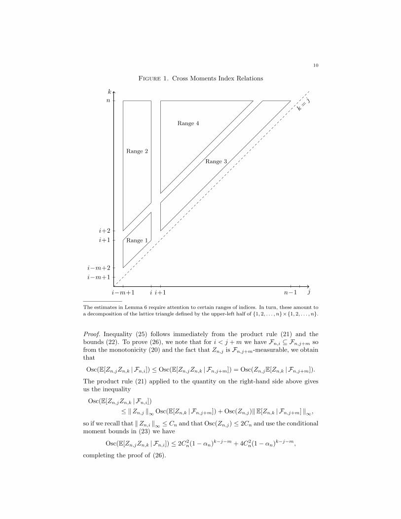
The minimal ergodic coefficient αn can also be used to control the oscillation ofthe conditional expectations of the products Zn,jZn,k given Fn,i. All of the inequal-ities that we need tell a similar story, but the specific bounds have an inescapabledependence on the relative values of i, j, k, n, and m. Figure 1 gives a graphicalrepresentation of the constraints on the indices that feature in the next lemma.

Lemma 6 (Conditional Cross Moments). For each i ∈ m, . . . , n+m we consideri−m < j < n and j < k ≤ n. We then have the following oscillation bounds thatdepend on the range of the indices (see also Figure 1):

Range 1. If j ≤ i and k ≤ j +m then

(25) Osc(E[Zn,jZn,k | Fn,i]) ≤ 4C2n.

Range 2. If j ≤ i < j +m < k then

(26) Osc(E[Zn,jZn,k | Fn,i]) ≤ 6C2n(1− αn)k−j−m.

Range 3. If i < j < k ≤ j +m then

(27) Osc(E[Zn,jZn,k | Fn,i]) ≤ 2C2n(1− αn)j−i.

Range 4. If i < j ≤ j +m < k, then

(28) Osc(E[Zn,jZn,k | Fn,i]) ≤ 6C2n(1− αn)k−i−m.

10

Figure 1. Cross Moments Index Relations

k

ji−m+1 i i+1 n−1

i−m+1

i−m+2

i+1

i+2

n

Range 1

Range 2

Range 3

Range 4

k=j

The estimates in Lemma 6 require attention to certain ranges of indices. In turn, these amount toa decomposition of the lattice triangle defined by the upper-left half of 1, 2, . . . , n×1, 2, . . . , n.

Proof. Inequality (25) follows immediately from the product rule (21) and thebounds (22). To prove (26), we note that for i < j +m we have Fn,i ⊆ Fn,j+m sofrom the monotonicity (20) and the fact that Zn,j is Fn,j+m-measurable, we obtainthat

Osc(E[Zn,jZn,k | Fn,i]) ≤ Osc(E[Zn,jZn,k | Fn,j+m]) = Osc(Zn,jE[Zn,k | Fn,j+m]).

The product rule (21) applied to the quantity on the right-hand side above givesus the inequality

Osc(E[Zn,jZn,k | Fn,i])≤ ‖Zn,j ‖∞Osc(E[Zn,k | Fn,j+m]) + Osc(Zn,j)‖E[Zn,k | Fn,j+m] ‖∞,

so if we recall that ‖Zn,i ‖∞ ≤ Cn and that Osc(Zn,j) ≤ 2Cn and use the conditionalmoment bounds in (23) we have

Osc(E[Zn,jZn,k | Fn,i]) ≤ 2C2n(1− αn)k−j−m + 4C2

n(1− αn)k−j−m,

completing the proof of (26).

11

To verify inequality (27), we consider the map Xn,j 7→ pj(Xn,j) given by

pj(Xn,j) = E[Zn,jZn,k | Fn,j ],

and we note that for i < j we have the pullback identity

E[Zn,jZn,k | Fn,i] = (K(n)i,j pj)(Xn,i).

Since ‖Zn,j ‖∞ and ‖Zn,k ‖∞ are bounded by Cn, we have ‖ pj ‖∞ ≤ C2n and

Osc(pj) ≤ 2C2n. We also have i < j < k so (12) tells us that

Osc(K(n)i,j pj) ≤ δ(K

(n)i,j ) Osc(pj) ≤ 2C2

n(1− αn)j−i,

completing the proof of (27).Finally, for the last inequality (28) we have j ≤ j +m < k, we consider the map

Xn,j 7→ qj(Xn,j) defined by setting

qj(Xn,j) = E[Zn,j(E[Zn,k | Fn,j+m]) | Fn,j ],

and we obtain the identity

E[Zn,jZn,k | Fn,i] = (K(n)i,j qj)(Xn,i).

By the multiplicative bound (12), this gives us

Osc(E[Zn,jZn,k | Fn,i]) ≤ (1− αn)j−i Osc(qj),

and we also have Osc(qj) ≤ 6C2n(1−αn)k−j−m by (26), so the proof of (28) is also

complete.

6. The Value To-Go Process and MDS L∞-Bounds

We have everything we need to argue that the variance condition (4) impliesthe negligibility condition (13). The first step is to get simple L∞-estimates of thevalue to-go Vn,i that was defined in (15). We then need estimates of the martingaledifferencedn,i defined in (16). Here, and subsequently, we use M = M(m) to denotea Hardy-style constant which depends only on m and which may change from oneline to the next.

Lemma 7 (L∞-Bounds for the Value To-Go and for the MDS). There is a constantM <∞ such that for all n ≥ 1 we have

‖Vn,i ‖∞ ≤MCnα−1n , for m ≤ i ≤ n+m, and(29)

‖ dn,i ‖∞ ≤MCnα−1n , for 1 +m ≤ i ≤ n+m.(30)

Proof. We have ‖Zn,j ‖∞ ≤ Cn, and when we use this estimate on the first msummands in the definition (15) of the value to-go Vn,i we get the bound

‖Vn,i ‖∞ ≤ mCn +

n∑j=i+1

‖E[Zn,j | Fn,i] ‖∞.

From (23) we know that ‖E[Zn,j | Fn,i] ‖∞ ≤ 2Cn(1− αn)j−i for all 1 ≤ i < j ≤ nso, after completing the geometric series, we have

‖Vn,i ‖∞ ≤ mCn + 2Cnα−1n ≤MCnα

−1n ,

where one can take M = 2m as a generous choice for M . This bound, the repre-sentation (16), and the triangle inequality then give us (30).

12

Conditional Variances L2-Bounds

Everything is also in place to show that the variance condition (4) gives one theweak law of large numbers for the conditional variances (14). We begin by derivingsome basic inequalities for the variance of Sn.

Lemma 8 (Variance Bounds). For all n ≥ 1 we have

(31) E[S2n] = E[V 2

n,m] +

n+m∑j=1+m

E[d2n,j ], and

(32) Var[Sn]−MC2nα−2n ≤

n+m∑j=1+m

E[d2n,j ] ≤ Var[Sn].

Proof. When we square both sides of (17) we have

S2n = V 2

n,m + 2Vn,m

n+m∑j=1+m

dn,j

+

n+m∑j=1+m

dn,j

2

.

Since Vn,m is Fn,m-measurable, we obtain from the conditional orthogonality of themartingale differences that

E[S2n | Fn,m] = V 2

n,m +

n+m∑j=1+m

E[d2n,j | Fn,m],

and, when we take the total expectation, we then get (31). Finally, since E[Sn] = 0,the representation (31) and the bound (29) for ‖Vn,m ‖∞ give us the two inequalitiesof (32).

Lemma 9 (Oscillation Bound). There is a constant M <∞ such that

(33) Osc(

n+m∑j=1+i

E[d2n,j | Fn,i]) ≤MC2

nα−2n for m ≤ i ≤ n+m.

Proof. If we sum the identity (16) we have

n+m∑j=1+i

Zn,j−m = Vn,i +

n+m∑j=1+i

dn,j ,

so, when we square both sides and use the fact that Vn,i is Fn,i-measurable, theorthogonality of the martingale differences gives us

E[ n+m∑

j=1+i

Zn,j−m2 | Fn,i

]= V 2

n,i +

n∑j=i+1

E[d2n,j | Fn,i].

The triangle inequality then implies

(34) Osc( n+m∑j=i+1

E[d2n,j | Fn,i]

)≤ Osc(V 2

n,i) + Osc(E[ n+m∑

j=1+i

Zn,j−m2 | Fn,i

]).

By (29) we have ‖Vn,i ‖∞ ≤MCnα−1n so, by (18), we obtain

(35) Osc(V 2n,i) ≤ 2‖V 2

n,i ‖∞ ≤MC2nα−2n .

13

It only remains to estimate the second summand of (34), but this takes somework. Specifically, we will check that one can write

(36) Osc(E[ n∑j=1+i−m

Zn,j2|Fn,i]) ≤ S0 + S1 + S2 + S3 + S4.

where S0,S1,S2,S3, and S4 are non-negative sums that one can estimate individu-ally with help from our oscillation bounds. Here the first term S0 accounts for theoscillation of the conditional squared moments. It is given by

S0 =

i∑j=1+i−m

Osc(E[Z2n,j |Fn,i]) +

n∑j=1+i

Osc(E[Z2n,j |Fn,i]),

and by (22) and (24) we have the estimate

S0 ≤ 2mC2n + 2C2

n

n∑j=1+i

(1− αn)j−i ≤ 2(1 +m)C2nα−1n .

The remaining sums S1,S2,S3 and S4 are given by the oscillation of the condi-tional cross moments Zn,jZn,k given Fn,i where the ranges of the indices j and kare given by the corresponding four regions in Figure 1. Specifically, we have

S1 = 2

i∑j=1+i−m

j+m∑k=1+j

Osc(E[Zn,jZn,k | Fn,i]),

and (25) gives us S1 ≤ 8m2C2n since S1 has m2 summands. Next, if we set

S2 = 2

i∑j=1+i−m

n∑k=1+j+m

Osc(E[Zn,jZn,k | Fn,i])

then the oscillation inequality (26) gives us

S2 ≤ 12C2n

i∑j=1+i−m

n∑k=1+j+m

(1− αn)k−j−m ≤ 12mC2nα−1n .

Similarly, for the third region, the bound (27) gives us

S3 = 2

n∑j=1+i

j+m∑k=1+j

Osc(E[Zn,jZn,k | Fn,i])

≤ 4C2n

n∑j=1+i

j+m∑k=1+j

(1− αn)j−i ≤ 4mC2nα−1n ,

and, for the fourth region, the bound (28) implies

S4 = 2

n∑j=1+i

n∑k=1+j+m

Osc(E[Zn,jZn,k | Fn,i])

≤ 12C2n

n∑j=1+i

n∑k=1+j+m

(1− αn)k−i−m ≤ 12C2nα−2n .

14

Finally, by our decomposition (36), the upper bounds for S0,S1,S2,S3, and S4 tellus that there is a constant M for which we have

Osc(E[ n∑j=1+i−m

Zn,j2|Fn,i]) ≤MC2

nα−2n ,

so, given (34) and (35), the proof of the lemma is complete.

7. Completion of the Proof of Theorem 1

It only remains to argue that if we set

ηi = E[d2n,i | Fn,i−1] and ∆n =

n+m∑i=1+m

(ηi − E[ηi]),

then the variance condition (4) implies that ∆n = o(Var[Sn]) in probability asn→∞. We can get this as an easy consequence of the next lemma.

Lemma 10 (L2-Bound for ∆n). There is a constant M < ∞ depending only onm such that for all n ≥ 1 one has the inequality

E[∆2n] = Var

[n+m∑i=1+m

E[d2n,i | Fn,i−1]

]≤MC2

nα−2n Var[Sn].

Proof. By direct expansion we have

(37) E[∆2n] =

n+m∑i=1+m

Var[ηi] + 2

n+m∑i=1+m

E[(ηi − E[ηi])

n+m∑j=i+1

(ηj − E[ηj ]

)],

and we estimate the two sums separately. First, by crude bounds and (30) we have

E[η2i ] ≤ ‖ ηi ‖∞ E[ηi] ≤ ‖ dn,i ‖2∞ E[ηi] ≤MC2

nα−2n E[ηi],

so we obtain that the first sum of (37) satisfies the inequality

n+m∑i=1+m

Var[ηi] ≤MC2nα−2n

n+m∑i=1+m

E[ηi].

The twin bounds of (32) and the definition ηi = E[d2n,i | Fn,i−1] then tell us that

(38) Var[Sn]−MC2nα−2n ≤

n+m∑i=1+m

E[ηi] ≤ Var[Sn],

so we also have the upper bound

(39)

n+m∑i=1+m

Var[ηi] ≤MC2nα−2n Var[Sn].

To estimate the second sum of (37), we first note that ηi is Fn,i−1-measurableand Fn,i−1 ⊆ Fn,i, so, if we condition on Fn,i we have

(40) E[(ηi−E[ηi])

n+m∑j=i+1

(ηj−E[ηj ])]

= E[(ηi−E[ηi])E[

n+m∑j=i+1

(ηj−E[ηj ]) | Fn,i]].

15

The definition of ηj tells us that ηj − E[ηj ] = E[d2n,j | Fn,j−1]− E[d2

n,j ] so, becauseFn,i ⊆ Fn,j−1 for all i < j, one then has

E[

n+m∑j=i+1

(ηj − E[ηj ]) | Fn,i] =

n+m∑j=i+1

E[d2n,j | Fn,i]− E[d2

n,j ].

These summands have mean zero, so the bound (19) and the oscillation inequality(33) give us

‖E[

n+m∑j=i+1

(ηj − E[ηj ])|Fn,i] ‖∞ ≤MC2nα−2n .

When we use this estimate in (40), we see from the non-negativity of ηj and thetriangle inequality that

‖E[(ηi − E[ηi])

n+m∑j=i+1

(ηj − E[ηj ])]‖∞ ≤MC2

nα−2n E[ηi],

so, after summing over i ∈ 1 +m, . . . , n+m and recalling the second inequalityof (38) we obtain

(41) ‖n+m∑i=1+m

E[(ηi − E[ηi])

n+m∑j=i+1

(ηj − E[ηj ])]‖∞ ≤MC2

nα−2n Var[Sn].

By (37), the bounds (39) and (41) complete the proof of the lemma.

Now, at last, we can use the basic decomposition (17) to write

(42)Sn√

Var[Sn]=

n∑i=1

dn,i+m√Var[Sn]

+O(‖Vn,m ‖∞√

Var[Sn]

),

and it only remains to apply our lemmas. First, from our hypothesis (4) thatC2nα−2n = o(Var[Sn]) as n → ∞, we see that the L∞-bound ‖ dn,i ‖∞ ≤ MCnα

−1n

in Lemma 7 implies the asymptotic negligibility (13) of the scaled differences

dn,i+m/√

Var[Sn], 1 ≤ i ≤ n. Second, our hypothesis (4) and the variance bounds(32) imply the asymptotic equivalence

Var[Sn] ∼n∑i=1

E[d2n,i+m] as n→∞,

so the L2-inequality in Lemma 10 tells us that the weak law (14) also holds for thescaled martingale differences.

Taken together, these two observations imply that the first sum on the right-handside of (42) converges in distribution to a standard normal. Moreover, becauseof the L∞-bound ‖Vn,m ‖∞ ≤ MCnα

−1n given by (29), the last term in (42) is

asymptotically negligible. In turn, these observations tell us that

Sn√Var[Sn]

=⇒ N(0, 1) as n→∞,

and the proof of Theorem 1 is complete.

16

8. Dynamic Inventory Management: A Leading Example

We now consider a classic dynamic inventory management problem where onehas n periods and n independent demands D1, D2, . . . , Dn. For the purpose ofillustration, we also assume that demand Di in period i has the uniform distributionon [0, a] for some a > 0, but this assumption is far from necessary.

In each period 1 ≤ i ≤ n one knows the current level of inventory x, and thetask is to decide the level of inventory y ≥ x that one wants to hold after an orderis placed and fulfilled. Here it is also useful to allow for x to be negative, and, inthat case, |x| would represent the level of backlogged demand. To stay mindful ofthis possibility, we sometimes call x the generalized inventory level.

We further assume that orders are fulfilled instantaneously at a cost that isproportional to the ordered quantity; so, for example, to move the inventory levelfrom x to y ≥ x, one places an order of size y− x and incurs a purchase cost equalto c(y − x) where the multiplicative constant c is a parameter of the model.

The model also takes into account the cost of either holding physical inventoryor of managing a backlog. Specifically, if the current generalized inventory is equalto x, then the firm incurs additional carrying costs that are given by

L(x) =

chx if x ≥ 0

−cpx if x < 0.

In other words, if x ≥ 0, then L(x) represents the cost for holding a quantity xof inventory from one period to the next, and, if x < 0, then L(x) represents thepenalty cost for managing a quantity −x ≥ 0 of unmet demand.

Here we also assume that all unmet demand can be successfully backlogged, socustomers in one period whose demand is incompletely met will return in successiveperiods until either their demand has been met or until the decision period n iscompleted. If there is still unmet demand at time n, then that demand is lost.Finally, we assume that the purchase cost rate c is strictly smaller than the penaltyrate cp, so it is never optimal to accrue penalty costs when one can place an order.Naturally, the manager’s objective is to minimize the total expected inventory costsover the decision periods 1, 2, . . . , n.

This problem has been widely studied, and, at this point, its formulation as adynamic program is well understood — cf. Bellman, Glicksberg and Gross (1955),Bulinskaya (1964), or Porteus (2002, Section 4.2). Specifically, if we let vk(x) denotethe minimal expected inventory cost when there are k time periods remaining andwhen x is the current generalized inventory level, then dynamic programming givesus the backwards recursion

(43) vk(x) = miny≥xc(y − x) + E[L(y −Dn−k+1)] + E[vk−1(y −Dn−k+1)],

for 1 ≤ k ≤ n, and one computes vk(x) by iteration beginning with v0(x) ≡ 0.It is also known that for this model there is a base-stock policy that is optimal;

that is, there are non-decreasing values

(44) s1 ≤ s2 ≤ · · · ≤ sn

17

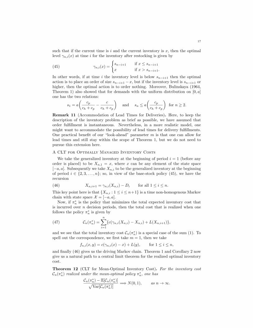
such that if the current time is i and the current inventory is x, then the optimallevel γn,i(x) at time i for the inventory after restocking is given by

(45) γn,i(x) =

sn−i+1 if x ≤ sn−i+1

x if x > sn−i+1.

In other words, if at time i the inventory level is below sn−i+1 then the optimalaction is to place an order of size sn−i+1− x, but if the inventory level is sn−i+1 orhigher, then the optimal action is to order nothing. Moreover, Bulinskaya (1964,Theorem 1) also showed that for demands with the uniform distribution on [0, a]one has the two relations:

s1 = a

(cp

ch + cp− c

ch + cp

)and sn ≤ a

(cp

ch + cp

)for n ≥ 2.

Remark 11 (Accommodation of Lead Times for Deliveries). Here, to keep thedescription of the inventory problem as brief as possible, we have assumed thatorder fulfillment is instantaneous. Nevertheless, in a more realistic model, onemight want to accommodate the possibility of lead times for delivery fulfillments.One practical benefit of our “look-ahead” parameter m is that one can allow forlead times and still stay within the scope of Theorem 1, but we do not need topursue this extension here.

A CLT for Optimally Managed Inventory Costs

We take the generalized inventory at the beginning of period i = 1 (before anyorder is placed) to be Xn,1 = x, where x can be any element of the state space[−a, a]. Subsequently we take Xn,i to be the generalized inventory at the beginningof period i ∈ 2, 3, . . . , n; so, in view of the base-stock policy (45), we have therecursion

(46) Xn,i+1 = γn,i(Xn,i)−Di for all 1 ≤ i ≤ n.This key point here is that Xn,i : 1 ≤ i ≤ n+1 is a time non-homogenous Markovchain with state space X = [−a, a].

Now, if π∗n is the policy that minimizes the total expected inventory cost thatis incurred over n decision periods, then the total cost that is realized when onefollows the policy π∗n is given by

(47) Cn(π∗n) =

n∑i=1

c(γn,i(Xn,i)−Xn,i) + L(Xn,i+1),

and we see that the total inventory cost Cn(π∗n) is a special case of the sum (1). Tospell out the correspondence, we first take m = 1, then we take

fn,i(x, y) = c(γn,i(x)− x) + L(y), for 1 ≤ i ≤ n,and finally (46) gives us the driving Markov chain. Theorem 1 and Corollary 2 nowgive us a natural path to a central limit theorem for the realized optimal inventorycost.

Theorem 12 (CLT for Mean-Optimal Inventory Cost). For the inventory costCn(π∗n) realized under the mean-optimal policy π∗n, one has

Cn(π∗n)− E[Cn(π∗n)]√Var[Cn(π∗n)]

=⇒ N(0, 1), as n→∞.

18

Two steps are used to extract this result from Theorem 1. First we show that theminimal ergodic coefficient of the Markov chain (46) is bounded away from zero,and, second, we show that the variance of Cn(π∗n) grows to infinity as n→∞.

Before we take these steps, we should explain why Theorem 12 does not followfrom Dobrushin’s theorem and the traditional device of state space extension. Thetrouble comes from the fact that when one extends the state space the coefficientof ergodicity can become degenerate.

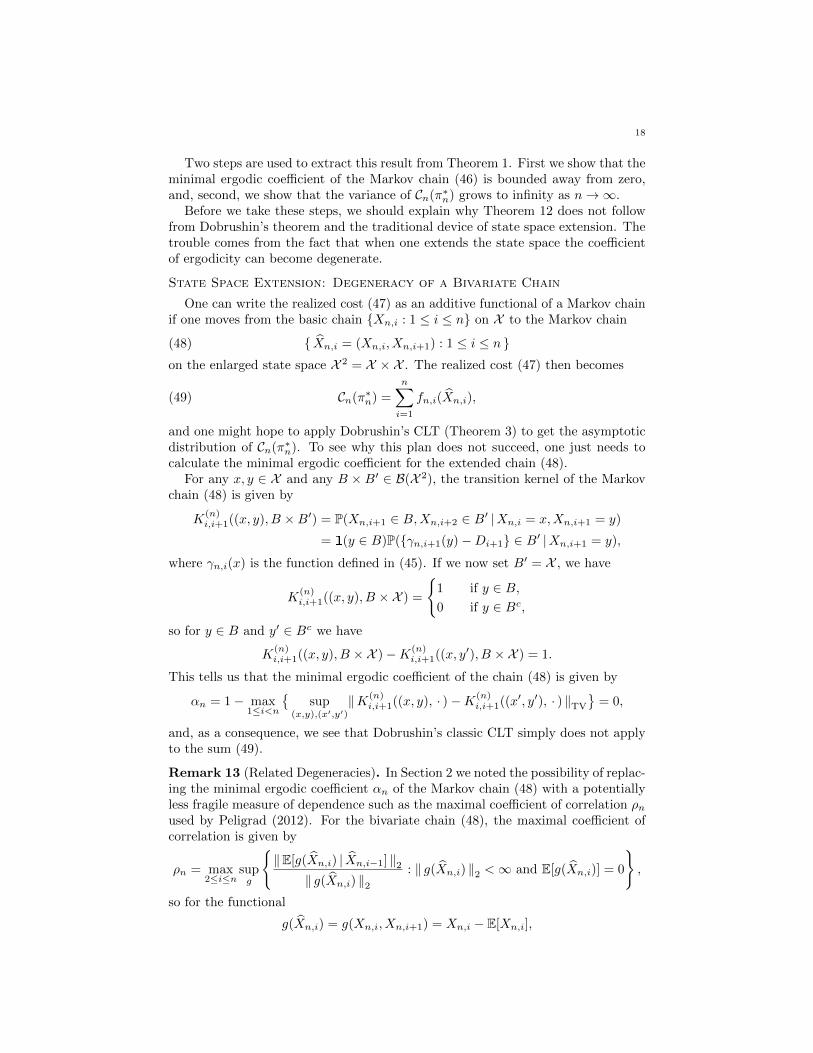
State Space Extension: Degeneracy of a Bivariate Chain

One can write the realized cost (47) as an additive functional of a Markov chainif one moves from the basic chain Xn,i : 1 ≤ i ≤ n on X to the Markov chain

(48) Xn,i = (Xn,i, Xn,i+1) : 1 ≤ i ≤ n on the enlarged state space X 2 = X × X . The realized cost (47) then becomes

(49) Cn(π∗n) =

n∑i=1

fn,i(Xn,i),

and one might hope to apply Dobrushin’s CLT (Theorem 3) to get the asymptoticdistribution of Cn(π∗n). To see why this plan does not succeed, one just needs tocalculate the minimal ergodic coefficient for the extended chain (48).

For any x, y ∈ X and any B × B′ ∈ B(X 2), the transition kernel of the Markovchain (48) is given by

K(n)i,i+1((x, y), B ×B′) = P(Xn,i+1 ∈ B,Xn,i+2 ∈ B′ |Xn,i = x,Xn,i+1 = y)

= 1(y ∈ B)P(γn,i+1(y)−Di+1 ∈ B′ |Xn,i+1 = y),

where γn,i(x) is the function defined in (45). If we now set B′ = X , we have

K(n)i,i+1((x, y), B ×X ) =

1 if y ∈ B,0 if y ∈ Bc,

so for y ∈ B and y′ ∈ Bc we have

K(n)i,i+1((x, y), B ×X )−K(n)

i,i+1((x, y′), B ×X ) = 1.

This tells us that the minimal ergodic coefficient of the chain (48) is given by

αn = 1− max1≤i<n

sup

(x,y),(x′,y′)

‖K(n)i,i+1((x, y), · )−K(n)

i,i+1((x′, y′), · ) ‖TV

= 0,

and, as a consequence, we see that Dobrushin’s classic CLT simply does not applyto the sum (49).

Remark 13 (Related Degeneracies). In Section 2 we noted the possibility of replac-ing the minimal ergodic coefficient αn of the Markov chain (48) with a potentiallyless fragile measure of dependence such as the maximal coefficient of correlation ρnused by Peligrad (2012). For the bivariate chain (48), the maximal coefficient ofcorrelation is given by

ρn = max2≤i≤n

supg

‖E[g(Xn,i) | Xn,i−1] ‖2

‖ g(Xn,i) ‖2: ‖ g(Xn,i) ‖2 <∞ and E[g(Xn,i)] = 0

,

so for the functional

g(Xn,i) = g(Xn,i, Xn,i+1) = Xn,i − E[Xn,i],

19

one has ρn = 1, and we see that the CLT of Peligrad (2012) does not help us here.

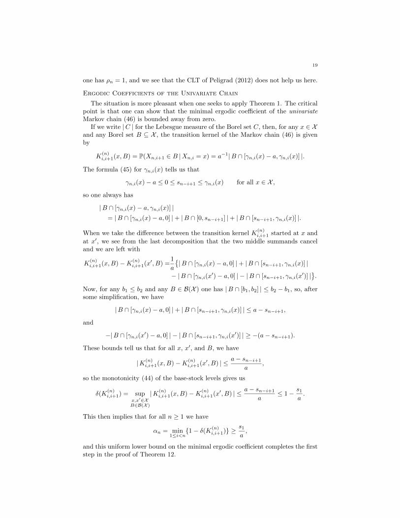
Ergodic Coefficients of the Univariate Chain

The situation is more pleasant when one seeks to apply Theorem 1. The criticalpoint is that one can show that the minimal ergodic coefficient of the univariateMarkov chain (46) is bounded away from zero.

If we write |C | for the Lebesgue measure of the Borel set C, then, for any x ∈ Xand any Borel set B ⊆ X , the transition kernel of the Markov chain (46) is givenby

K(n)i,i+1(x,B) = P(Xn,i+1 ∈ B |Xn,i = x) = a−1|B ∩ [γn,i(x)− a, γn,i(x)] |.

The formula (45) for γn,i(x) tells us that

γn,i(x)− a ≤ 0 ≤ sn−i+1 ≤ γn,i(x) for all x ∈ X ,

so one always has

|B ∩ [γn,i(x)− a, γn,i(x)] |= |B ∩ [γn,i(x)− a, 0] |+ |B ∩ [0, sn−i+1] |+ |B ∩ [sn−i+1, γn,i(x)] |.

When we take the difference between the transition kernel K(n)i,i+1 started at x and

at x′, we see from the last decomposition that the two middle summands canceland we are left with

K(n)i,i+1(x,B)−K(n)

i,i+1(x′, B) =1

a

|B ∩ [γn,i(x)− a, 0] |+ |B ∩ [sn−i+1, γn,i(x)] |

− |B ∩ [γn,i(x′)− a, 0] | − |B ∩ [sn−i+1, γn,i(x

′)] |.

Now, for any b1 ≤ b2 and any B ∈ B(X ) one has |B ∩ [b1, b2] | ≤ b2 − b1, so, aftersome simplification, we have

|B ∩ [γn,i(x)− a, 0] |+ |B ∩ [sn−i+1, γn,i(x)] | ≤ a− sn−i+1,

and

−|B ∩ [γn,i(x′)− a, 0] | − |B ∩ [sn−i+1, γn,i(x

′)] | ≥ −(a− sn−i+1).

These bounds tell us that for all x, x′, and B, we have

|K(n)i,i+1(x,B)−K(n)

i,i+1(x′, B) | ≤ a− sn−i+1

a,

so the monotonicity (44) of the base-stock levels gives us

δ(K(n)i,i+1) = sup

x,x′∈XB∈B(X )

|K(n)i,i+1(x,B)−K(n)

i,i+1(x′, B) | ≤ a− sn−i+1

a≤ 1− s1

a.

This then implies that for all n ≥ 1 we have

αn = min1≤i<n

1− δ(K(n)i,i+1) ≥ s1

a,

and this uniform lower bound on the minimal ergodic coefficient completes the firststep in the proof of Theorem 12.

20

Variance Lower Bound

Here, as in most stochastic dynamic programs, the value to-go process (15) canbe expressed in terms of the value functions that solve the dynamic programmingrecursion (43). In particular, at time 1 ≤ i ≤ n, when the current generalizedinventory is Xn,i and there are n− i+ 1 demands yet to be realized, one has

Vn,i = vn−i+1(Xn,i),

where the function x 7→ vn−i+1(x) is calculated by (43). Moreover, since we startwith Xn,1 = x, the definition of vn(x) gives us

Vn,1 = vn(x) = E[Cn(π∗n)],

and the martingale decomposition (17) can be written more explicitly as

Cn(π∗n)− E[Cn(π∗n)] =

n∑i=1

dn,i+1.

To estimate Var[Cn(π∗n)] from below, we just need to find an appropriate lowerbound on E[d2

n,i+1] for 1 ≤ i ≤ n. In our inventory problem we begin by writingthe martingale differences (16) more explicitly as

(50) dn,i+1 = c(γn,i(Xn,i)−Xn,i) + L(Xn,i+1) + vn−i(Xn,i+1)− vn−i+1(Xn,i).

Next, we introduce the shorthand vn−i(x) = L(x)+vn−i(x), and we obtain fromthe recursion (43) and the policy characterization (45) that

vn−i+1(x) = c(γn,i(x)− x) + E[L(γn,i(x)−Di)] + E[vn−i(γn,i(x)−Di)](51)

= c(γn,i(x)− x) + E[vn−i(γn,i(x)−Di)].

We now replace x with Xn,i in (51) to get a new expression for vn−i+1(Xn,i),and we replace the last summand of (50) with this expression. If we recall from(46) that Xn,i+1 = γn,i(Xn,i)−Di, then we find after simplification that

dn,i+1 = vn−i(γn,i(Xn,i)−Di)− E[vn−i(γn,i(Xn,i)−Di) | Fn,i],

where, just as before, one has Fn,i = σXn,1, Xn,2, . . . , Xn,i. This representationgives us a key starting point for estimating the second moment of dn,i+1.

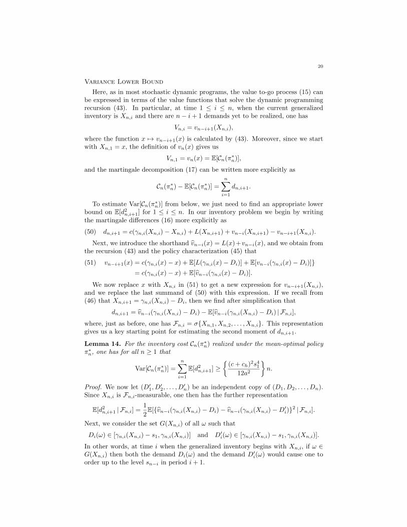
Lemma 14. For the inventory cost Cn(π∗n) realized under the mean-optimal policyπ∗n, one has for all n ≥ 1 that

Var[Cn(π∗n)] =

n∑i=1

E[d2n,i+1] ≥

(c+ ch)2s4

1

12a2

n.

Proof. We now let (D′1, D′2, . . . , D

′n) be an independent copy of (D1, D2, . . . , Dn).

Since Xn,i is Fn,i-measurable, one then has the further representation

E[d2n,i+1 | Fn,i] =

1

2E[vn−i(γn,i(Xn,i)−Di)− vn−i(γn,i(Xn,i)−D′i)2 | Fn,i].

Next, we consider the set G(Xn,i) of all ω such that

Di(ω) ∈ [γn,i(Xn,i)− s1, γn,i(Xn,i)] and D′i(ω) ∈ [γn,i(Xn,i)− s1, γn,i(Xn,i)].

In other words, at time i when the generalized inventory begins with Xn,i, if ω ∈G(Xn,i) then both the demand Di(ω) and the demand D′i(ω) would cause one toorder up to the level sn−i in period i+ 1.

21

If we now replace i with i+ 1 in the recursion (51) we see that

vn−i(x)− vn−i(y)1((x, y) ∈ [0, s1]2) = (c+ ch)(y − x)1((x, y) ∈ [0, s1]2),

because the two new inventory levels for the next period i + 1 are both givenby γn,i+1(x) = γn,i+1(y) = sn−i and because one incurs holding costs that areproportional to the difference y − x. This last equivalence implies the lower bound

E[d2n,i+1 | Fn,i] ≥

1

2(c+ ch)2E[D′i −Di21(G(Xn,i)) | Fn,i].

We now recall that Di and D′i are independent and uniformly distributed on [0, a]and integrate the right-hand side to obtain that

E[d2n,i+1 | Fn,i] ≥

(c+ ch)2s41

12a2> 0.

After one takes the total expectation and sums over 1 ≤ i ≤ n, the proof of thelemma is complete.

9. An Application in Combinatorial Optimization:Online Alternating Subsequences

Given a sequence y1, y2, . . . , yn of n distinct real numbers, we say that a subse-quence yi1 , yi2 , . . . , yik , 1 ≤ i1 < i2 < · · · < ik ≤ n, is alternating provided that therelative magnitudes alternate as in

yi1 < yi2 > yi3 < yi4 > · · · or yi1 > yi2 < yi3 > yi4 < · · · .

Combinatorial investigations of alternating subsequences go back to Euler (cf.Stanley, 2010), but probabilistic investigations are more recent; Widom (2006),Pemantle (cf. Stanley, 2007, p. 568), Stanley (2008) and Houdre and Restrepo(2010) all considered the distribution of the length of the longest alternating subse-quence of a random permutation or of a sequence Y1, Y2, . . . , Yn of independentrandom variables with the uniform distribution on [0, 1]. There have also beenrecent applications of this work in computer science (e.g. Romik, 2011; Bannisterand Eppstein, 2012) and in tests of independence (cf. Brockwell and Davis, 2006,p. 312).

Here we consider alternating subsequences in a sequential, or online, contextwhere we are presented with the values Y1, Y2, . . . , Yn one at the time, and the goalis to select an alternating subsequence

(52) Yτ1 < Yτ2 > Yτ3 < Yτ4 > · · · ≶ Yτkthat has maximal expected length.

A sequence of selection times 1 ≤ τ1 < τ2 < · · · < τk ≤ n that satisfy (52)is called a feasible policy if our decision to accept or reject Yi as member ofthe alternating subsequence is based only on our knowledge of the observationsY1, Y2, . . . , Yi. In more formal terms, the feasibility of a policy is equivalent torequiring that the indices τk, k = 1, 2, . . ., are all stopping times with respect tothe increasing sequence of σ-fields Ai = σY1, Y2, . . . , Yi, 1 ≤ i ≤ n.

We now let Π denote the set of all feasible policies, and for π ∈ Π, we let Aon(π) bethe number of alternating selections made by π for the realization Y1, Y2, . . . , Yn,so

Aon(π) = max k : Yτ1 < Yτ2 > · · · ≶ Yτk and 1 ≤ τ1 < τ2 < · · · < τk ≤ n .

22

We say that a policy π∗n ∈ Π is optimal (or, more precisely, mean-optimal) if

E[Aon(π∗n)] = supπ∈Π

E[Aon(π)].

Arlotto, Chen, Shepp and Steele (2011) found that for each n there is a uniquemean-optimal policy π∗n such that

E[Aon(π∗n)] = (2−√

2)n+O(1),

and it was later found that there is a CLT for Aon(π∗n).

Theorem 15 (CLT for Optimal Number of Alternating Selections). For the mean-optimal number of alternating selections Aon(π∗n) one has

Aon(π∗n)− E[Aon(π∗n)]√Var[Aon(π∗n)]

=⇒ N(0, 1) as n→∞.

The main goal of this section is to show that Theorem 1 leads to a proof of thistheorem that is quicker, more robust, and more principled than the original proofgiven in Arlotto and Steele (2014). In the process, we also get a second illustrationof the ways in which Theorem 1 helps one sidestep the degeneracy that sometimesarises when one tries to use Dobrushin’s theorem on a naturally associated bivariatechain. In fact, it is this feature of Dobrushin’s theorem that initially motivated thedevelopment of Theorem 1.

Structure of the Additive Process

To formulate the alternating subsequence problem as an MDP, we first considera new state space that consists of pairs (x, s) where x denotes the value of thelast selected observation and where we set s = 0 if x is a local minimum and sets = 1 if x is a local maximum. The decision problem then has a notable reflectionproperty: the optimal expected number of alternating selections that one makeswhen k observations are yet to be seen is the same if the system is in state (x, 0)or if the system is in state (1 − x, 1). Earlier analyses exploited this symmetry toshow that there is a sequence gk : 1 ≤ k <∞ of optimal threshold functions suchthat if one sets Xn,1 = 0 and lets

(53) Xn,i+1 =

Xn,i if Yi < gn−i+1(Xn,i)

1− Yi if Yi ≥ gn−i+1(Xn,i),

then the optimal number of alternating selections has the representation

(54) Aon(π∗n) =

n∑i=1

1 (Yi ≥ gn−i+1(Xn,i)) =

n∑i=1

1(Xn,i+1 6= Xn,i).

The derivation of these relations requires a substantial amount of work, but forthe purpose of illustrating Theorem 1 and Corollary 2, one does not need to gointo the details of the construction of these optimal threshold functions. Here it isenough to note that this representation for Aon(π∗n) is exactly of the form (1) thatis addressed by Theorem 1.

The proof of Theorem 15 then takes two steps. First, one needs an appropriatelower bound for the minimal ergodic coefficients of the chain (53), and second oneneeds to check that the variance of Aon(π∗n) goes to infinity as n→∞.

The second property is almost baked into the cake, and it is even proved inArlotto and Steele (2014) that Var[Aon(π∗n)] grows linearly with n. Still, to keep our

23

discussion brief, we will not repeat that proof. Instead we focus on the new — andmore strategic — fact that minimal ergodic coefficients of the Markov chains (53)are uniformly bounded away from zero for all 1 ≤ i ≤ n− 2 and all n ≥ 3.

A Lower Bound for the Minimal Ergodic Coefficient

For any x ∈ [0, 1] and any Borel set B ⊆ [0, 1], the Markov chain (53) has thetransition kernel

K(n)i,i+1(x,B) = 1(x ∈ B)gn−i+1(x) +

∫ 1

gn−i+1(x)

1(1− u ∈ B) du

= 1(x ∈ B)gn−i+1(x) + |B ∩ [0, 1− gn−i+1(x)] |,where the first summand of the top equation accounts for the rejection of the newlypresented value Yi = u, and the second summand accounts for its acceptance.

To obtain a meaningful estimate for the contraction coefficient of K(n)i,i+1 we recall

from the earlier analyses that the optimal threshold functions gk : 1 ≤ k < ∞have the two basic properties: (i) gk(x) = x for all x ∈ [1/3, 1] and all k ≥ 1, and(ii) gk(x) ≥ 1/6 for all x ∈ [0, 1] and all k ≥ 3. Property (ii) and the recursion (53)give us Xn,i ≤ 5/6 for all 1 ≤ i ≤ n− 2, and we see from property (i) that

δ(K(n)i,i+1) = sup

x,x′‖K(n)

i,i+1(x, ·)−K(n)i,i+1(x′, ·) ‖TV ≤

5

6for all 1 ≤ i ≤ n− 2.

This estimate gives us in turn that

αn−2 = min1≤i<n−2

1− δ(K(n)i,i+1) ≥ 1

6,

so by Corollary 2 we have the CLT for Aon−2(π∗n). Since Aon(π∗n) and Aon−2(π∗n)differ by at most 2, this also completes the proof of Theorem 15.

10. A Final Observation

Theorem 1 generalizes the classical CLT of Dobrushin (1956), and it offers a pre-packaged approach to the CLT for the kinds of additive functionals that one meetsin the theory of finite horizon Markov decision processes. The technology of MDPsis wedded to the pursuit of policies that maximize total expected rewards, butsuch policies may not make good economic sense unless the realized reward is “wellbehaved.” While there are several ways to characterize good behavior, asymptoticnormality of the realized reward is likely to be high on almost anyone’s list. Theorientation of Theorem 1 addresses this issue in a direct and practical way.

The examples of Sections 8 and 9 illustrate more concretely what one needs todo to apply Theorem 1. In a nutshell, one needs to show that the variance of thetotal reward goes to infinity and one needs an a priori lower bound on the minimalcoefficient of ergodicity. These conditions are not trivial, but, as the examples show,they are not intractable. Now, whenever one faces the question of a CLT for thetotal reward of a finite horizon MDP, there is an explicit agenda that lays out whatone needs to do.

References

Arlotto, A., Chen, R. W., Shepp, L. A. and Steele, J. M. (2011), ‘Online selection of alternating

subsequences from a random sample’, J. Appl. Probab. 48(4), 1114–1132.Arlotto, A., Gans, N. and Steele, J. M. (2014), ‘Markov decision problems where means bound

variances’, Oper. Res. 62(4), 864–875.

24

Arlotto, A. and Steele, J. M. (2014), ‘Optimal online selection of an alternating subsequence: a

central limit theorem’, Adv. in Appl. Probab. 46(2), 536–559.

Bannister, M. J. and Eppstein, D. (2012), Randomized speedup of the Bellman–Ford algorithm,in ‘Proceedings of the Meeting on Analytic Algorithmics & Combinatorics, Kyoto, Japan,

January 16, 2012’, Society for Industrial and Applied Mathematics, Philadelphia, PA, pp. 41–

47.Bellman, R., Glicksberg, I. and Gross, O. (1955), ‘On the optimal inventory equation’, Manage-

ment Sci. 2, 83–104.

Brockwell, P. J. and Davis, R. A. (2006), Time series: theory and methods, Springer Series inStatistics, Springer, New York. Reprint of the second (1991) edition.

Brown, B. M. (1971), ‘Martingale central limit theorems’, Ann. Math. Statist. 42, 59–66.

Bulinskaya, E. V. (1964), ‘Some results concerning optimum inventory policies’, Theory of Prob-ability & Its Applications 9(3), 389–403.

Del Moral, P. (2004), Feynman-Kac formulae, Probability and its Applications (New York),Springer-Verlag, New York.

Dobrushin, R. L. (1956), ‘Central limit theorem for nonstationary Markov chains. I, II’, Theory

of Probability & Its Applications 1(1), 65–80; ibid. 1(4), 329–383.Gordin, M. I. (1969), ‘The central limit theorem for stationary processes’, Dokl. Akad. Nauk SSSR

188, 739–741.

Gordin, M. and Peligrad, M. (2011), ‘On the functional central limit theorem via martingaleapproximation’, Bernoulli 17(1), 424–440.

Hall, P. and Heyde, C. C. (1980), Martingale limit theory and its application, Academic Press,

Inc., New York-London.Hanen, A. (1963), ‘Theoremes limites pour une suite de chaınes de Markov’, Ann. Inst. H.

Poincare 18, 197–301.

Houdre, C. and Restrepo, R. (2010), ‘A probabilistic approach to the asymptotics of the length ofthe longest alternating subsequence’, Electron. J. Combin. 17(1), Research Paper 168, 1–19.

Iosifescu, M. and Theodorescu, R. (1969), Random processes and learning, Springer-Verlag, NewYork.

Kifer, Y. (1998), ‘Limit theorems for random transformations and processes in random environ-

ments’, Trans. Amer. Math. Soc. 350(4), 1481–1518.Kipnis, C. and Varadhan, S. R. S. (1986), ‘Central limit theorem for additive functionals of

reversible Markov processes and applications to simple exclusions’, Comm. Math. Phys.

104(1), 1–19.Mandl, P. (1973), ‘A connection between controlled Markov chains and martingales’, Kybernetika

(Prague) 9, 237–241.

Mandl, P. (1974a), ‘Estimation and control in Markov chains’, Adv. in Appl. Probab. 6, 40–60.Mandl, P. (1974b), On the asymptotic normality of the reward in a controlled Markov chain,

in ‘Progress in statistics (European Meeting Statisticians, Budapest, 1972), Vol. II’, North-

Holland, Amsterdam, pp. 499–505. Colloq. Math. Soc. Janos Bolyai, Vol. 9.Mandl, P. (1985), ‘Local asymptotic normality in controlled Markov chains’, Statist. Decisions

2, 123–127. Selected papers presented at the 16th European meeting of statisticians (Marburg,1984).

Mandl, P. and Lausmanova, M. (1991), ‘Two extensions of asymptotic methods in controlled

Markov chains’, Ann. Oper. Res. 28(1-4), 67–79.McLeish, D. L. (1974), ‘Dependent central limit theorems and invariance principles’, Ann. Probab.

2, 620–628.Mendoza-Perez, A. F. (2008), ‘Asymptotic normality of average cost Markov control processes’,

Morfismos 12, 33–52.

Mendoza-Perez, A. F. and Hernandez-Lerma, O. (2010), ‘Asymptotic normality of discrete-time

Markov control processes’, J. Appl. Probab. 47(3), 778–795.Peligrad, M. (2012), ‘Central limit theorem for triangular arrays of non-homogeneous Markov

chains’, Probab. Theory Related Fields 154(3-4), 409–428.Porteus, E. (2002), Foundations of Stochastic Inventory Theory, Business/Marketing, Stanford

University Press.

25

Romik, D. (2011), Local extrema in random permutations and the structure of longest alternating

subsequences, in ‘23rd International Conference on Formal Power Series and Algebraic Com-

binatorics (FPSAC 2011)’, Discrete Math. Theor. Comput. Sci. Proc., AO, Assoc. DiscreteMath. Theor. Comput. Sci., Nancy, pp. 825–834.

Sarymsakov, T. A. (1961), ‘Inhomogeneous Markov chains’, Theory of Probability & Its Applica-

tions 6(2), 178–185.Seneta, E. (2006), Non-negative matrices and Markov chains, Springer Series in Statistics,

Springer, New York. Revised reprint of the second (1981) edition.

Sethuraman, S. and Varadhan, S. R. S. (2005), ‘A martingale proof of Dobrushin’s theorem fornon-homogeneous Markov chains’, Electron. J. Probab. 10, no. 36, 1221–1235 (electronic).

Stanley, R. P. (2007), Increasing and decreasing subsequences and their variants, in ‘International

Congress of Mathematicians. Vol. I’, Eur. Math. Soc., Zurich, pp. 545–579.Stanley, R. P. (2008), ‘Longest alternating subsequences of permutations’, Michigan Math. J.

57, 675–687. Special volume in honor of Melvin Hochster.Stanley, R. P. (2010), ‘A survey of alternating permutations’, Contemp. Math. 531, 165–196.

Statuljavicus, V. A. (1969), ‘Limit theorems for sums of random variables that are connected in

a Markov chain. I, II, III’, Litovsk. Mat. Sb. 9, 345–362; ibid. 9, 635–672; ibid. 10, 161–169.Szewczak, Z. S. (2012), ‘On Dobrushin’s inequality’, Statist. Probab. Lett. 82(6), 1202–1207.

Widom, H. (2006), ‘On the limiting distribution for the length of the longest alternating sequence

in a random permutation’, Electron. J. Combin. 13(1), Research Paper 25, 1–7.Winkler, G. (2003), Image analysis, random fields and Markov chain Monte Carlo methods,

Vol. 27 of Applications of Mathematics (New York), second edn, Springer-Verlag, Berlin.

Wu, W. B. and Woodroofe, M. (2004), ‘Martingale approximations for sums of stationary pro-cesses’, Ann. Probab. 32(2), 1674–1690.