climate impacts of intermittent upper ocean mixing induced

Climate impacts of intermittent upper ocean mixing inducedby tropical cyclones

G. E. Manucharyan,1 C. M. Brierley,1 and A. V. Fedorov1

Received 17 May 2011; revised 16 August 2011; accepted 17 August 2011; published 29 November 2011.

[1] Tropical cyclones (TC) represent a powerful, albeit highly transient forcing able toredistribute ocean heat content locally. Recent studies suggest that TC‐induced oceanmixing can have global climate impacts as well, including changes in poleward heattransport, ocean circulation, and thermal structure. In several previous modeling studiesdevoted to this problem, the TC mixing was treated as a permanent (constant in time)source of additional vertical diffusion in the upper ocean. In contrast, this study aims toexplore the highly intermittent character of the mixing. We present results from a seriesof coupled climate experiments with different durations of the imposed intermittentmixing but where each has the same annual mean diffusivity. All simulations show robustchanges in sea surface temperature and ocean subsurface temperature, independent ofthe duration of the mixing that varies between the experiments from a few days to a fullyear. Simulated temperature anomalies are characterized by a cooling in the subtropics,a moderate warming in middle to high latitudes, a pronounced warming of the equatorialcold tongue, and a deepening of the tropical thermocline. These effects are paralleled bysubstantial changes in ocean and atmosphere circulation and heat transports. While thegeneral patterns of changes remain the same from one experiment to the next, theirmagnitude depends on the relative duration of the mixing. Stronger mixing, but of ashorter duration, has less of an impact. These results agree with a simple model of heattransfer for the upper ocean with a time‐dependent vertical diffusivity.

Citation: Manucharyan, G. E., C. M. Brierley, and A. V. Fedorov (2011), Climate impacts of intermittent upper ocean mixinginduced by tropical cyclones, J. Geophys. Res., 116, C11038, doi:10.1029/2011JC007295.

1. Introduction

[2] Tropical cyclones (TC), also called hurricanes andtyphoons, are some of the most destructive weather systemson Earth. Their intense winds cause vigorous ocean verticalmixing [D’Asaro et al., 2007] that brings colder water to thesurface while pumping warm surface waters downward.Experiments with ocean models [Sriver et al., 2010] showthat strong storms can induce vertical mixing to depths of250 m and result in a cooling of 6°C or more in the storm’swake. It has been argued that this vertical mixing may haveglobal climate impacts by contributing to oceanic polewardheat transport [Emanuel, 2001; Sriver and Huber, 2007] andbymodifying ocean circulation and thermal structure [Fedorovet al., 2010]. The overarching goal of the present study is toinvestigate further the climate impacts of this mixing in acomprehensive coupled general circulation model (GCM).Attempts to quantify the amount of TC mixing from obser-vations have found that tropical cyclones induce an annualmean diffusivity in the range of 1 cm2/s [Sriver and Huber,

2007; Sriver et al., 2008] to 6 cm2/s [Liu et al., 2008].What effects could this additional mixing have on climate?[3] Using observed tracks of tropical cyclones and a

simplified ocean model, Emanuel [2001] estimated thatTC‐induced mixing contributes 1.4 ± 0.7 PW in oceanpoleward heat transport (1 PW = 1015 W), which representsa substantial fraction of the observed heat transport by theoceans. He concluded that tropical cyclones might play animportant role in driving the ocean thermohaline circulationand thereby regulating climate. Sriver and Huber [2007] andSriver et al. [2008] generally supported this conclusion butdowngraded heat transport estimates to about 0.3–0.5 PW.[4] Using an ocean GCM, Jansen and Ferrari [2009]

demonstrated that an equatorial gap in the TC mixing regionaltered the structure of the TC‐generated heat transports,allowing for a heat convergence toward the equator. On theother hand, Jansen et al. [2010] suggested that the climateeffects of mixing by TC could be strongly reduced by sea-sonal factors, namely, by the heat release to the atmospherein winter (this argument was based on the assumption thatthe mixing did not penetrate significantly below the seasonalthermocline).[5] Hu and Meehl [2009] investigated the effect of hur-

ricanes on the Atlantic meridional overturning circulation(AMOC) using a relatively coarse global coupled GCM in

1Department of Geology and Geophysics, Yale University, New Haven,Connecticut, USA.

Copyright 2011 by the American Geophysical Union.0148‐0227/11/2011JC007295

JOURNAL OF GEOPHYSICAL RESEARCH, VOL. 116, C11038, doi:10.1029/2011JC007295, 2011

C11038 1 of 13

http://dx.doi.org/10.1029/2011JC007295

which tropical cyclones in the Atlantic were included viaprescribed winds and precipitation. Their conclusion wasthat the strength of the AMOC in the model would increaseif hurricane winds were taken into account; however,changes in precipitation due to hurricanes would have anopposite effect. More recently, Scoccimarro et al. [2011]used a TC‐permitting coupled GCM and estimated thecontribution of TC to the annually averaged ocean heattransport an order of magnitude smaller than suggested bySriver and Huber [2007] and Sriver et al. [2008]. Their model,however, was too coarse to fully resolve tropical storms,leading to the simulated TC activity about 50% weaker withfewer strong storms than are observed.[6] Korty et al. [2008] developed an intermediate‐

complexity coupled model with a TC parameterization in theform of interactive mixing in the upper ocean that dependedon the state of the coupled system. The main aim of the studywas to investigate the potential role of tropical cyclones insustaining equable climates, such as the warm climate of theEocene epoch. These authors noted a significant increase inTC‐induced ocean mixing in a warmer climate, an increasein poleward heat transport, and a corresponding warming ofhigh latitudes.[7] Fedorov et al. [2010] implemented a constant addi-

tional mixing within two zonal subtropical bands that theyadded to the upper ocean vertical diffusivity in a compre-hensive climate GCM. They describe a mechanism in whichTC warm water parcels are advected by the wind drivencirculation and resurface in the eastern equatorial Pacific,warming the equatorial cold tongue by 2°C–3°C, deepeningthe tropical thermocline, and reducing the zonal SST gradientalong the equator. This leads to El Niño‐like climate con-ditions in the Pacific and changes in the atmospheric cir-culation (the Walker and the Hadley cells). While the goalof this study was to simulate the climate state of the earlyPliocene [Fedorov et al., 2006], these results have muchbroader implications for the role of tropical cyclones inmodern climate.[8] The conclusions of Fedorov et al. [2010] generally

agree with those of Sriver and Huber [2010], who addedhigh‐resolution winds from observations to an ocean model,and those of Pasquero and Emanuel [2008], who modeledthe propagation of oceanic temperature anomalies created bya single instantaneous mixing event. The latter authors foundthat at least one third of the warm subsurface temperatureanomaly was advected by wind‐driven circulation toward theequator, which should lead to an increase in ocean heatcontent in the tropics. In parallel, the impact of small latitu-dinal variations in background vertical mixing (unrelated toTC) was investigated in a coupled climate model by Jochum[2009], who concluded that the equatorial ocean is one of theregions most sensitive to spatial variations in diffusivity.[9] Several of the aforementioned modeling studies param-

etrize the effect of tropical storms by adding annual meanvalues of the TC‐induced diffusivity inferred from observa-tions to the background vertical diffusivity already used in anocean model. However, a single tropical cyclone inducesmixing of a few orders of magnitudes greater than the annualmean value. Thus, a question naturally arises: how reliableare results obtained by representing a time‐varying mixingwith its annual mean value? To that end, the goal of thisstudy is to explore the role of intermittency (i.e., temporal

dependence) of the upper ocean mixing in a coupled climatemodel.[10] Note that previously, Boos et al. [2004] argued that a

transient mixing could affect the ocean thermohaline cir-culation, especially if the mixing was applied near the oceanboundaries. However, their study was performed in an oceanonly model with TC mixing penetrating to the bottom of theocean.[11] In our study, to mimic the effects of tropical cyclones,

we use several representative cases of time‐dependent mixingthat yield the same annual mean values of vertical diffusivity.The approach remains relatively idealized, in line with thestudies of Jansen and Ferrari [2009] and Fedorov et al.[2010]. A spatially uniform (but time varying) mixing isimposed in zonal bands in the upper ocean. We analyzechanges in sea surface temperatures (SST), oceanic thermalstructure, the meridional overturning circulation in the oceanand the atmosphere, and poleward heat transports.[12] In addition, we formulate a simple one‐dimensional

model of heat transfer to understand the sensitivity of the SSTand heat transport to the duration of mixing. It accounts forthe gross thermal structure of the upper ocean and incorporatestime‐dependent coefficients of vertical diffusivity. Usingthis simple model, we vary the fraction of the year withTC‐induced mixing and look at the ocean response. Both thecomprehensive and simple models suggest that highly inter-mittent mixing should generate a response 30%–40% weakerthan from a permanent mixing of the same average value.

2. Climate Model and Experiments

[13] We explore the global climate impacts of upper oceanmixing induced by tropical cyclones using the CommunityClimate System Model, version 3 (CCSM3) [Collins et al.,2006]. The ocean component of CCM3 has 40 vertical levels,a 1.25° zonal resolution, and a varying meridional resolutionwith a maximum grid size of 1° that reduces to 0.25° in theequatorial region. The atmosphere has 26 vertical levels and ahorizontal spectral resolution of T42 (roughly 2.8° × 2.8°).The atmosphere and other components of the model, such assea ice and land surface, are coupled to the ocean every 24 h.[14] The conventional vertical mixing of tracers in the ocean

model is given by (1) a background diffusivity (0.1 cm2/s inthe upper ocean) attributable to the breaking of internal waveswhich is constant in time [Danabasoglu et al., 2006] and(2) a diffusivity due to shear instabilities, convection, anddouble‐diffusion processes parameterized by the KPP scheme[Large et al., 1994], which varies in time and space. Theannual mean SST and thermal structure of the upper Pacificfor this climate model are shown in Figure 1.[15] To incorporate the effects of tropical cyclones into the

model, we add extra vertical diffusivity in the upper oceanwithin the subtropical bands, defined here as 8°N–40°N and8°S–40°S (Figure 1). This additional diffusivity can varywith time throughout the year but maintains an annual meanvalue of 1 cm2/s (10 times larger than the model’s back-ground diffusivity). This mean value, when applied every-where in the subtropical bands, is probably an overestimationfor the present climate; however, TC‐induced diffusivitymay have been even greater in past warm climates [Kortyet al., 2008].

MANUCHARYAN ET AL.: INTERMITTENT MIXING BY TROPICAL CYCLONES C11038C11038

2 of 13

[16] The imposed diffusivity is spatially uniform, follow-ing the studies of Jansen and Ferrari [2009] and Fedorovet al. [2010], who looked at the gross effects of TC mixingin the subtropical bands and neglected zonal variations inthe mixing. We ignore buoyancy effects associated withincreased precipitation and heat fluxes generated by TC at theocean surface [Hu and Meehl, 2009; Scoccimarro et al.,2011] and focus solely on the mixing effects.[17] Our choice for the average depth to which TC mixing

penetrates is 200 m. In nature, this depth varies significantlydepending on the local ocean stratification and the char-acteristics of a particular storm. Nonetheless, 200 m appearsto be a reasonable value for a number of applications. Forexample, mixing induced by hurricane Frances in the Atlanticpenetrated to about 130 m depth, as measured in the hurri-cane wake by a deployed array of sea floats [D’Asaro et al.,2007]. However, mixing generated by typhoon Kirogi in theWestern Pacific may have penetrated to depths of about500 m with the strongest effects concentrated in the upper250 m, as estimated from calculations with an ocean GCMforced by observed winds [Sriver, 2010]. Using a simplemodel for TC‐induced mixing, Korty et al. [2008] estimated

the penetration depth at about 200 m for their experimentwith moderate concentration of CO2 in the atmosphere andat 300 m for their warm climate.[18] We perform four perturbed model experiments with

different temporal dependence of TC‐induced mixing, and acontrol run with no additional mixing. In the experimentreferred to as “permanent,” we specify a diffusivity thatremains constant throughout the year. In the other threeperturbation experiments the temporal dependence of themixing is given by step functions alternating between onand off stages. In the “seasonal” experiment a constantmixing is applied only for half a year. In the “single‐event”experiment mixing occurs once a year and lasts only 5 days.The “multiple‐event” experiment represents six major TC ayear that last 2 days each (Figure 2 and Table 1). To takeinto account the seasonality of tropical cyclone activity,TC mixing in these three experiments is imposed only duringthe warm part of the year in each hemisphere (summer andfall) with a half year lag between different hemispheres.[19] We emphasize that in all perturbed cases the annual

mean value of TC‐induced diffusivity remains the same(1 cm2/s, similar to that estimated by Sriver and Huber

Figure 1. (a) The annual mean sea surface temperature and (b) the upper‐ocean temperature along 180°W.Both plots are for the control simulation. In the perturbation experiments, additional mixing is imposed inthe zonal bands 8°N–40°N and 8°S–40°S in the upper 200 m of the ocean, as indicated by the shading.


3 of 13

[2007]). Consequently, peak values of the imposed verticaldiffusivity for highly intermittent mixing exceed diffusivityfor permanent mixing by two orders of magnitude (Table 1).[20] For each perturbed experiment the model is initialized

from a 1000 year simulation with preindustrial conditionsand spun up for 200 years after introducing the time‐varyingvertical diffusivity. Similarly, our control experiment is a200 year continuation of the preindustrial simulation. Theresults of the experiments will be presented in terms ofanomalies from the control run, averaged over the last25 years of calculations.

3. Results From the Climate Model

3.1. The Time Scales of Climate Response

[21] We start the discussion of the model results with thetime series of several essential climate indexes that show thetransient response of the climate system to introducedmixing.The time evolution of global mean temperature and the meantop‐of‐the‐atmosphere (TOA) radiation flux indicates thatthe climate system is adjusting to changes in the ocean dif-fusivity with an e‐folding time scale of nearly 30 years(Figures 3a and 3b). After 100 years these variables do notchange, except for weak decadal variations. Initially, we seea drop in global mean temperatures and a counteractingincrease in the TOA radiation flux. However, as the TOAradiation imbalance diminishes, the global mean temperatureincreases and settles at a value slightly greater than in thecontrol run (by 0.1°C–0.2°C). This increase seems to berobust between different experiments, even though its mag-

nitude is comparable with the internal variability of thecontrol run.[22] Furthermore, the time series of Niño 3.4 index

(indicative of the tropical ocean response) show that a warmtemperature anomaly of substantial magnitude emerges alongthe equator also within the first 30 years of simulations(Figure 3c). This indicates that the initial time scales of theclimate response are set by the adjustment of the wind‐drivencirculation and thermal structure of the upper ocean, thatoccurs on time scales of 20–40 years [Harper, 2000; Barreiroet al., 2008] controlled by a combination of advective, waveand diabatic processes [Boccaletti et al., 2004; Fedorov et al.,2004].[23] In contrast to the first three indexes, the index of the

AMOC intensity, related to the deep ocean circulation, showsa sharp decrease after the additional mixing was imposed,but then follows a very slow recovery (Figure 3d). Thedeep ocean continues its adjustment on longer time scales(centennial to millennial) that should involve diapycnal dif-fusion throughout the global ocean [Wunsch and Heimbach,2008] and processes in the Southern Ocean [Haertel andFedorov, 2011; Allison et al., 2011].[24] Nevertheless, roughly after 100 years of simulation,

the atmosphere and the upper ocean have gone through theirinitial adjustment stages and are now experiencing a slowresidual climate drift (because of the deep ocean adjustment)as well as decadal variability. We thus focus our discussionson the dynamics of the upper ocean and the atmosphere, butavoid making final conclusions on the state of the AMOC(also see section 5).

Figure 2. The duration and magnitude of the added vertical diffusivity that replicates TC‐induced oceanmixing in different experiments with the climate model (permanent, seasonal, multiple‐event, and single‐event experiments). The regions where this additional mixing is imposed in perturbation experiments areshown in Figure 1. For further details, see Table 1.

Table 1. The Main Characteristics and Results of Different Perturbation Experimentsa

Mixing Cases Ton Toff Dmax (cm2/s) OHT (PW) SSTb (°C) SSTct (°C) Tgm (°C) a

Permanent 12 months 0 months 1 0.12 −0.19 2.3 0.11 1.00Seasonal 6 months 6 months 2 0.21 −0.30 2.2 0.09 0.99Multiple events 2 days 28 day 30 0.16 −0.14 1.7 0.19 0.72Single event 5 days 360 days 73 0.13 −0.03 1.7 0.09 0.62

aDuration of the imposed mixing (Ton, Toff), maximum values of the imposed vertical diffusivity (Dmax), peak anomalies in ocean heat transport (OHT),mean SST cooling within the mixing bands (SSTb), the maximum warming of the cold tongue (SSTct), anomalies in global mean surface air temperature(Tgm), and the regression coefficient (a) for SST anomalies in the transient mixing experiments with respect to those in the permanent mixing run. Allproperties are the average of the last 25 years of simulation, except the coefficient a, which is the average of the last 100 years.


4 of 13

3.2. Climate Response

[25] All four perturbation experiments produce similarpatterns of SST anomalies generated by TC‐induced mixing(Figure 4) independent of the exact temporal dependence ofthe mixing: a weak surface cooling at the location of mixingand a warming in other regions (middle and high latitudesand the equatorial region). The cooling is caused by a greaterlocal entrainment of colder waters from below and pumpingof warm surface waters into the interior of the ocean bythe additional mixing [Jansen and Ferrari, 2009; Sriver et al.,2008; Sriver and Huber, 2010]. In turn, the warming iscaused by the advection of these relatively warm waters,

pumped down by mixing, and their subsequent upwellingto the surface away from the source regions. The warmingis amplified by atmospheric feedbacks (see below). Theoverall pattern of the SST response to the anomalous mixingis similar to that noted in previous works [Fedorov et al.,2010; Sriver and Huber, 2010].[26] The largest SST cooling in themixing bands is achieved

for the seasonal experiment with an average reduction of0.3°C and local values reaching 1°C (Figure 4). Seasonalmixing causes a stronger SST change than the permanentmixing, because vertical mixing is more efficient in modify-ing the SSTs during summer, when the thermal stratification

Figure 3. The time evolution of (a) global mean temperature, (b) top‐of‐the‐atmosphere radiationimbalance, (c) the Niño 3.4 SST, and (d) the volume transport of the Atlantic meridional overturning circu-lation (AMOC) in different experiments, including the control run (orange line), as simulated by the climatemodel. A 25 year runningmean has been applied. Note that the atmospheric data were saved only for the last150 years of the control simulation.


5 of 13

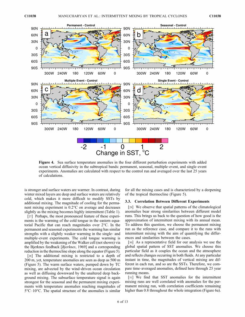
is stronger and surface waters are warmer. In contrast, duringwinter mixed layers are deep and surface waters are relativelycold, which makes it more difficult to modify SSTs byadditional mixing. The magnitude of cooling for the perma-nent mixing experiment is 0.2°C on average and decreasesslightly as the mixing becomes highly intermittent (Table 1).[27] Perhaps, the most pronounced feature of these experi-

ments is the warming of the cold tongue in the eastern equa-torial Pacific that can reach magnitudes over 2°C. In thepermanent and seasonal experiments the warming has similarstrengths with a slightly weaker warming in the single‐ andmultiple‐event experiments. The cold tongue warming isamplified by the weakening of theWalker cell (not shown) viathe Bjerknes feedback [Bjerknes, 1969] and a correspondingreduction in the thermocline slope along the equator (Figure 5).[28] The additional mixing is restricted to a depth of

200 m, yet, temperature anomalies are seen as deep as 500 m(Figure 5). The warm surface waters, pumped down by TCmixing, are advected by the wind‐driven ocean circulationas well as diffusing downward by the unaltered deep back-ground mixing. The subsurface temperature signal is againstrongest for the seasonal and the permanent mixing experi-ments with temperature anomalies reaching magnitudes of5°C–10°C. The spatial structure of the anomalies is similar

for all the mixing cases and is characterized by a deepeningof the tropical thermocline (Figure 5).

3.3. Correlation Between Different Experiments

[29] We observe that spatial patterns of the climatologicalanomalies bear strong similarities between different modelruns. This brings us back to the question of how good is theapproximation of intermittent mixing with its annual mean.To address this question, we choose the permanent mixingrun as the reference case, and compare it to the runs withintermittent mixing with the aim of quantifying the differ-ences and similarities between the cases.[30] As a representative field for our analysis we use the

global spatial pattern of SST anomalies. We choose thisparticular field as it couples the ocean and the atmosphereand reflects changes occurring in both fluids. At any particularinstant in time, the magnitudes of vertical mixing are dif-ferent in each run, and so are the SSTs. Therefore, we com-pare time‐averaged anomalies, defined here through 25 yearrunning means.[31] We find that SST anomalies for the intermittent

mixing runs are well correlated with anomalies for the per-manent mixing run, with correlation coefficients remaininghigher than 0.8 throughout the whole integration (Figure 6a).

Figure 4. Sea surface temperature anomalies in the four different perturbation experiments with addedocean vertical diffusivity in the subtropical bands: permanent, seasonal, multiple‐event, and single‐eventexperiments. Anomalies are calculated with respect to the control run and averaged over the last 25 yearsof calculations.


6 of 13

Figure 5. Ocean temperature anomalies as a function of depth (a–d) along the equator and (e–h) along180°W for different perturbation experiments. From top to bottom: permanent, seasonal, multiple‐event,and single‐event experiments. The solid and dashed black lines denote the position of the 20°C isotherm(a proxy for the tropical thermocline depth) in the perturbation experiments and the control run, respectively.Note the deepening of the tropical thermocline, the reduction of the thermocline slope along the equator, andthe strong subsurface temperature anomalies that extend to depths of about 500 m. Ocean diffusivity is mod-ified in the upper 200 m in the subtropical bands, 8°N–40°N and 8°S–40°S (regions shaded gray). Anomaliesare calculated with respect to the control run and averaged over the last 25 years of calculations.


7 of 13

Although all the runs experience a climate drift as well aslow‐frequency variability, these variations occur in a corre-lated way. Furthermore, the correlation coefficients haveno negative trends, implying that decorrelation time scalebetween different runs (if decorrelation does occur) is muchlonger than the 200 year integration time.[32] The fact that the spatial fields are well correlated,

allows us to calculate the relative magnitudes of SST anoma-lies in the intermittent mixing experiments with respect toSST anomalies for permanent mixing. We assume the fol-lowing relation between SST anomalies for each run:

DSST ¼ �DSSTperm þ err; ð1Þ

where DSST and DSSTperm are SST anomalies for differentintermittent mixing runs and for the permanent mixing run,respectively, a is the relative magnitude of the anomaly,and err is the error of such approximation. The regressioncoefficient a is computed as

� ¼ hDSST DSSTpermihDSSTpermDSSTpermi ; ð2Þ

where the operator h i denotes a dot product between thetwo fields (weighted by the surface area). When computingthese coefficients we actually subtract the means (relativelysmall) from the SST anomalies. Obviously, for the permanentmixing experiment, a = 1 and err ≡ 0. For the intermittentmixing experiments, a shows the relative magnitude of SSTanomalies with respect to the permanent mixing run.[33] These coefficients stay relatively constant in time after

the initial adjustment period (Figure 6b), which allows us toevaluate the relative magnitude of SST anomalies in different

experiments. Accordingly, anomalies in the seasonal experi-ment have almost the same magnitude as the permanent case(a ≈ 1). The multiple‐event and single‐event experimentsshow relative magnitudes of 72% and 62%, respectively,over the last 100 years (Table 1). The root‐mean‐square errorof such a representation lies between 0.2°C–0.3°C for the

Figure 6. (a) Temporal changes of the correlation coeffi-cients computed between annual mean SST anomalies inthe transient mixing experiments and those in the permanentmixing run. (b) The same as in Figure 6a, but for the regres-sion coefficient a. These coefficients indicate how close toeach other the SST anomalies in different experiments are.

Figure 7. Anomalous northward heat transport (NHT) by(a) the ocean, (b) the atmosphere, and (c) the entire ocean‐atmosphere system for different perturbation experiments.Thick gray lines on the horizontal axis indicate the latitudinalextent of the regions with enhanced mixing; the magnitudeof decadal changes in the heat transports does not exceed0.05 PW.


8 of 13

whole duration of the experiments, which implies thatapproximating the gross effects of intermittent mixing withappropriately scaled permanent mixing will produce a rela-tively small error (which is a factor of 2 or 3 smaller than thenatural decadal variability of SST anomalies).

3.4. Oceanic and Atmospheric OverturningCirculations and Heat Transports

[34] Changes in ocean temperatures are paralleled byanomalies in surface heat fluxes and hence in ocean polewardheat transport (Figure 7). The ocean heat uptake increases inthe regions of additional mixing, which results in two majoreffects: a stronger ocean heat transport to middle and highlatitudes (as suggested by Emanuel [2001]) and anomalousheat convergence toward the equator (as noted by Jansenand Ferrari [2009] and Fedorov et al. [2010]). The strongestocean heat transport anomalies are produced by seasonalmixing; it is harder to distinguish between the other casesbecause of decadal variability. The peak anomalous heattransport by the ocean reaches 0.15–0.25 PW, which roughlymatches the estimates by Sriver and Huber [2007].[35] The observed increase in ocean heat transport is

largely due to changes in the amount of heat transported bythe shallow wind‐driven circulation, rather than the deepoverturning circulation. In fact, we observe an initial weak-ening of the AMOC (Figure 3d) possibly caused by the sur-face warming of the Norwegian sea (Figure 4) which has astabilizing effect on convection. However, the integration timeof our experiments is not sufficient to reach an equilibrium, andat the end of 200 year simulation the AMOC still exhibits atrend toward higher values. Whether the AMOC eventuallyreturns to its undisturbed strength, or perhaps intensifies inagreement with the hypothesis of Emanuel [2001], is unclear.A definite answer to this question will require several thou-sand years of calculations.[36] It is important that SST changes, specifically an

increase in the meridional temperature gradient between thesubtropics and the equatorial region, cause the intensificationof the atmospheric Hadley circulation (Figure 8). As a result,anomalies in oceanic heat transport are partially compensatedby the atmosphere (Figure 7) in a manner reminiscent ofBjerknes compensation [Bjerknes, 1964; Shaffrey and Sutton,2006]. For example, whereas the ocean carries more heattoward the equator, the stronger Hadley circulation transportsmore heat away from the equator. Consequently, changes inoceanic heat transport of nearly 0.3 PW do not necessarilyrepresent changes in the total heat transport by the system(Figure 7c), which stays below 0.1 PW.[37] Nevertheless, a substantial fraction of oceanic heat

transport remains uncompensated as a stronger polewardheat transport by the ocean induces the atmospheric watervapor feedback in mid to high latitudes and a decrease inglobal albedo related to changes in low clouds and/or sea ice[Herweijer et al., 2005]. Such changes result in a slightincrease of global mean temperature (0.1°C–0.2°C) in all theexperiments with enhanced mixing (Table 1).[38] Finally, one of the consequences of the stronger winds

associated with the more intense Hadley circulation is thestrengthening of the ocean shallow overturning circulation,i.e., the subtropical cells (STC) in Figure 8. This strength-ening of the STC appears to moderate the warming of the

equatorial cold tongue but is not able to reverse ocean heatconvergence toward the equator.

4. A Simple Model for the Upper OceanThermal Structure With TC Mixing

4.1. Formulation of the Model

[39] To investigate further the ocean sensitivity to inter-mittent mixing, here we formulate a simple one‐dimensionalmodel describing the gross thermal structure of the upperocean when subjected to anomalous mixing events. Themodel equations for the vertical temperature profile in thesubtropical ocean T = T(z, t) are as follows:

Tt ¼ �Tzð Þz�� T � T*ð Þ; ð3aÞ�Tz ¼ ��s T � Tsð Þ; z ¼ 0; ð3bÞ

�Tz ¼ �b T � Tbð Þ; z ¼ �H : ð3cÞ[40] This is a heat transfer equation with horizontal

advection parameterized as a restoring term, −g(T − T*).The restoring time scale, g−1 = 10 year, is chosen to rep-resent advection by the wind‐driven subtropical cell (STC) inthe Pacific. The upstream temperature profile T* is obtainedas a steady state solution of equation (1) with a constantbackground diffusivity, �0, and no advective restoring. Thus,the restoring profile T* is also a steady state solution of thefull system, which will be used as the background profile tocompare solutions corresponding to different forms of inter-mittent mixing. In the coupled climate model both thestrength of the circulation and the upstream profile change alittle in response to the additional mixing, but we will neglectsuch effects here.[41] Atmospheric heat fluxes at the ocean surface are

parameterized by restoring the surface temperature to a pre-scribed atmospheric temperature, Ts (30°C). At the bottom ofthe integration domain (H = 300 m), the temperature isrestored to a deep ocean temperature, Td (10°C), which isset by the deep ocean circulation. The restoring time scales(or piston velocities [e.g., Griffies et al., 2005]) are as

−1 =0.3 m/d at the surface and ad

−1 = 0.08 m/d at the bottom ofthe domain. These values are chosen in such a way that asurface temperature anomaly caused by a mixing eventwould be restored roughly within two weeks and temper-ature anomalies at the bottom of the domain within twomonths (in terms of e‐folding time scales).[42] The time‐dependent vertical diffusivity consists of

two components: a background diffusivity, �0 (0.1 cm2/s)and an intermittent diffusivity, �′(t), replicating the effect ofTC (with the annual mean value of 1 cm2/s above 200 m,zero below). For simplicity, we neglect the seasonal cycleand restrict the form of �′(t) to a periodic step function withan on/off behavior:

�′ t þ �ð Þ ¼ �′ tð Þ ¼�on; 0 < t � r�;

0; r� < t � �:

8<: ð4Þ

The period, t, of the TC‐induced diffusivity is chosen to be1 year, yielding one event per year. The parameter r is ameasure of the mixing intermittency; it indicates the fraction


9 of 13

of the year that the TC mixing is on. Note that additionalvertical diffusivity during the on stage (�on) is normalizedby r, so that the annual mean diffusivity stays constant forall experiments.[43] The parameter r provides a link to the coupled model

simulations, in which r = 1 for the permanent case, r = 0.5for the seasonal, and r = 0.01 for the single‐event case (themultiple‐event case does not have a direct analogue in thisframework). The model is integrated numerically for a broadrange of parameter r (between 0.003 and 1) using a finitedifference scheme with a vertical resolution of 5 m and an

adaptive time step. Each experiment lasts for 200 years tomatch the coupled model experiments and to insure thatstatistical properties of this system are equilibrated.

4.2. Idealized Model Results

[44] The steady state solution of equation (3) without addi-tional diffusion describes an ocean with a linearly decreasingtemperature (Figure 9a, dashed line). Adding permanent dif-fusivity (r = 1) in the upper 200m leads to a substantial coolingat the surface and a warming at depth (Figure 9a, solid blackline). Note, that warm anomalies penetrate to depths below

Figure 8. (a, b) The zonally averaged atmospheric and oceanic circulations in the control run (the Hadleycells and the ocean shallow subtropical cells, respectively) and their anomalies in the (c, d) permanent mix-ing and (e, f) single‐event experiments. Note the strengthening of both the atmospheric and shallow oceanicmeridional overturning cells. Anomalies are averaged over the last 25 years of calculations.


10 of 13

200 m where no additional mixing is applied. This is a resultof slow diffusion due to the model original background dif-fusivity. The penetration depth (Lp) is dictated by the balancebetween vertical diffusion and advective restoring with thefollowing scaling: Lp ∼

ffiffiffiffiffiffiffiffiffiffi�0=�

p. This gives a penetration

depth of 170m below the additional mixing, which is in roughagreement with the climate model, where strong temperatureanomalies are observed at depths of 400–500 m.[45] When the additional diffusivity varies with time (r < 1),

so does the temperature profile. During the interval when thetransient mixing is on, the temperature profile becomes moreuniform with depth (Figure 9a, dark blue line). However,during the off stage this profile gradually relaxes toward theundisturbed temperature distribution (Figure 9a, light blue

line). Thus, the intermittent mixing causes large oscillationsin ocean temperature. When averaged, these oscillationsproduce persistent cold anomalies at the ocean surface andwarm anomalies at depth. The horizontal advection of thesewarm subsurface temperature anomalies generates anoma-lous heat transport (DHF), which eventually leads to thewarming in the equatorial cold tongue and of middle and highlatitudes.[46] The largest SST cooling (DSST) is achieved for

constant TC mixing (r = 1). As the mixing becomes moreintermittent (r < 1), the magnitude of the SST changedecreases (Figure 9b, blue line). In the limit of very small r(highly intermittent mixing), the average SST anomaly isreduced roughly by 30%–40%, but nevertheless remainssignificant; that is, short but strong mixing events are indeedimportant. The magnitude of the anomalous heat transportfollows roughly the same dependence on r (Figure 9b,red line).[47] Overall, such behavior is consistent with the coupled

model, implying that TC‐induced climate changes aredirectly related to thermal anomalies generated locally by TCmixing. The magnitude of the changes depends on howintermittent the mixing is, but only to a moderate extent. Boththe simple and coupled climate models suggest that para-meterizations of TC as a source of permanent mixing maylead to an overestimation of climate impacts of tropicalcyclones, but will have the correct spatial pattern.

5. Discussions and Conclusions

[48] This study investigates the global climate impacts oftemporally variable upper ocean mixing induced by tropicalcyclones using a global ocean‐atmosphere coupled modeland a simple heat transfer model of the upper ocean. Thetime‐averaged temperature anomalies in the coupled modelshow robust spatial patterns in response to additional verticalmixing. Specifically, we observe a weak surface cooling atthe location of the mixing (∼0.3°C), a strong warming of theequatorial cold tongue (∼2°C), and a moderate warming inmiddle to high latitudes (0.5°C–1°C). We also observe adeepening of the tropical thermocline with subsurface tem-perature anomalies extending to 500 m. These and otherchanges, summarized in Table 1, are consistent between thedifferent experiments.[49] Additional mixing leads to an enhanced oceanic heat

transport (on the order of 0.2 PW) from the regions ofincreased mixing toward high latitudes and the equatorialregion. This effect is partially compensated by the atmo-sphere, resulting in smaller changes in the total heat transport.An increase of the ocean poleward heat transport agrees withthe original idea of Emanuel [2001]. However, it is largelydue to the transport by the wind‐driven, rather than thethermohaline, circulation. There is also a small increase inglobalmean temperature (∼0.2°C), associatedwith the greaterocean heat transport (for a discussion, see Herweijer et al.[2005]).[50] The magnitude of the climate response to enhanced

mixing depends not only on the time‐averaged value of theadded diffusivity, but also on its temporal dependence. In ourcoupled climate model, a single‐event mixing produces aroughly 40% weaker response than permanent mixing (withthe same annual mean diffusivity). This result is reproduced

Figure 9. (a) Temperature profiles as a function of depthobtained as solutions of the simple one‐dimensional modelwith no additional mixing (dashed line) and with the addi-tion of permanent mixing (solid black line). For comparison,also shown are temperature profiles for an experiment withr = 0.05 directly after the mixing event (dark blue line) andafter the restoring period (light blue line). (b) Anomalies insurface temperature and implied ocean heat transport esti-mated from the simple model for different values of theparameter r. The mean value of the imposed diffusivity(1 cm2/s) remains the same for all r.


11 of 13

by our simple one‐dimensional heat transfer model for theupper ocean with a time‐dependent vertical diffusivity. Thesimple model shows a similar reduction of the local SSTanomaly and the anomalous heat transport from the mixingregion when we decrease the fraction of the year with mixing.[51] The presence of the seasonal cycle in the coupled

model amplifies the impact of tropical cyclones as they occurduring summer, when warm surface temperatures are favor-able for pumping heat into the interior of the ocean. In ourcoupled model this effect apparently overcomes the effect ofseasonality described by Jansen et al. [2010], who empha-sized heat release from the ocean back to the atmosphereduring winter that could weaken ocean thermal anomalies.Their mechanism appears to be more important for relativelyweak cyclones generating shallow mixing, and not forstronger cyclones that contribute to the mixing most.[52] To address the issue of the model dependency of our

conclusions we performed several additional experimentswith the Community Earth SystemModel (CESM), which is anewer version of the model that we used initially (CCSM3).Important differences between the models include the imple-mentation of the near surface eddy flux parameterization[Ferrari et al., 2008;Danabasoglu et al., 2008] and a new seaice component in CESM. Also, we used a lower‐resolutionversion of the newmodel as compared to CCSM3. The resultsof the new experiments are very similar to the prior experi-ments, showing the equatorial warming and the deepeningof the thermocline, the cooling of the subtropical bands, andthe strengthening of the shallow overturning circulation in theocean and the Hadley cells in the atmosphere. The patternsof generated climatological SST anomalies remain well cor-related between different mixing runs, with highly intermittentmixing having a somewhat weaker response. The only majordifference concerns the AMOC behavior and SST changes inthe high‐latitude northern Atlantic; in the new model theAMOC intensity does not change in response to additionalmixing. The persistent warming of the Norwegian Sea,observed in CCSM, is replaced by a surface cooling balancedby a density compensating freshwater anomaly. These effectsare probably due to the new sea ice model or the lower modelresolution; the question of their robustness goes beyond thescope of the present paper.[53] The consistent spatial patterns of the climate response

to transient mixing suggest that in coupled climate simulationsa highly intermittent upper ocean mixing can be representedby adding permanent or constant seasonal mixing, perhapsrescaled appropriately.[54] Several other relevant questions remain beyond the

scope of this study, including the role of spatial variations ofthe TC‐induced mixing and the adiabatic effects of theircyclonic winds on oceanic circulation through Ekmanupwelling. It is also feasible that for present‐day climate ourresults actually give the upper bound on the climate responseto tropical cyclones. A critical issue is the average depth ofmixing penetration; choosing a depth significantly shallowerthan 200 m for the experiments would dampen the overallsignal. Restricting the zonal extent of the mixing bands ineach ocean basin, more in line with observations, would alsoreduce the signal.[55] Ultimately, simulations with TC‐resolving climate

models will be necessary to fully understand the role oftropical cyclones in climate. However, the current generation

of GCMs are only slowly approaching this limit and are stillunable to reproduce many characteristics of the observedhurricanes, especially of the strongest storms critical for theocean mixing [e.g., Gualdi et al., 2008; Scoccimarro et al.,2011; P. L. Vidale, personal communication, 2011].

[56] Acknowledgments. This research was supported in part bygrants from NSF (OCE0901921), Department of Energy Office of Science(DE‐FG02‐08ER64590), and the David and Lucile Packard Foundation.Resources of the National Energy Research Scientific Computing Centersupported by the DOE under contract DE‐AC02‐05CH11231 are alsoacknowledged. We thank K. Emanuel and two anonymous reviewers forhelpful comments and suggestions.

ReferencesAllison, L., H. Johnson, and D. Marshall (2011), Spin‐up and adjustment ofthe Antarctic Circumpolar Current and global pycnocline, J. Mar. Res.,in press.

Barreiro, M., A. Fedorov, R. Pacanowski, and S. Philander (2008), Abruptclimate changes: How freshening of the Northern Atlantic affects thethermohaline and wind‐driven oceanic circulations, Annu. Rev. EarthPlanet. Sci., 36, 33–58.

Bjerknes, J. (1964), Atlantic air‐sea interaction, Adv. Geophys., 10(1), 1–82.Bjerknes, J. (1969), Atmospheric teleconnections from the equatorialPacific, Mon. Weather Rev., 97(3), 163–172.

Boccaletti, G., R. Pacanowski, S. Philander, and A. Fedorov (2004), Thethermal structure of the upper ocean, J. Phys. Oceanogr., 34(4), 888–902.

Boos, W., J. Scott, and K. Emanuel, (2004), Transient diapycnal mixingand the meridional overturning circulation, J. Phys. Oceanogr., 34(1),334–341.

Collins, W., et al. (2006), The Community Climate System Model version 3(CCSM3), J. Clim., 19, 2122–2143.

Danabasoglu, G., W. G. Large, J. J. Tribbia, P. R. Gent, B. P. Briegleb, andJ. C. McWilliams (2006), Diurnal coupling in the tropical oceans ofCCSM3, J. Clim., 19, 2347–2365.

Danabasoglu, G., R. Ferrari, and J. McWilliams (2008), Sensitivity of anocean general circulation model to a parameterization of near‐surfaceeddy fluxes, J. Clim., 21, 1192–1208.

D’Asaro, E., T. Sanford, P. Niiler, and E. Terrill (2007), Cold wake ofHurricane Frances, Geophys. Res. Lett., 34, L15609, doi:10.1029/2007GL030160.

Emanuel, K. (2001), Contribution of tropical cyclones to meridional heattransport by the oceans, J. Geophys. Res., 106, 14,771–14,781.

Fedorov, A., R. Pacanowski, S. Philander, and G. Boccaletti (2004), Theeffect of salinity on the wind‐driven circulation and the thermal structureof the upper ocean, J. Phys. Oceanogr., 34(9), 1949–1966.

Fedorov, A., P. Dekens,M.McCarthy, A. Ravelo, P. DeMenocal, M. Barreiro,R. Pacanowski, and S. Philander (2006), The Pliocene paradox (mechanismsfor a permanent El Nino), Science, 312(5779), 1485–1489.

Fedorov, A., C. Brierley, and K. Emanuel (2010), Tropical cyclones andpermanent El Niño in the early Pliocene epoch, Nature, 463, 1066–1070.

Ferrari, R., J. McWilliams, V. Canuto, and M. Dubovikov (2008), Parame-terization of eddy fluxes near oceanic boundaries, J. Clim., 21, 2770–2789.

Griffies, S., et al. (2005), Formulation of an ocean model for global climatesimulations, Ocean Sci., 1(1), 45–79.

Gualdi, S., et al. (2008), Changes in tropical cyclone activity due to globalwarming: Results from a high‐resolution coupled general circulationmodel, J. Clim., 21, 5204–5228.

Haertel, P., and A. Fedorov (2011), The ventilated ocean, J. Phys. Oceanogr.,doi:10.1175/2011JPO4590.1, in press.

Harper, S. (2000), Thermocline ventilation and pathways of tropical‐subtropical water mass exchange, Tellus, Ser. A, 52(3), 330–345.

Herweijer, C., R. Seager, M. Winton, and A. Clement (2005), Why oceanheat transport warms the global mean climate, Tellus, Ser. A, 57(4),662–675.

Hu, A., and G. Meehl (2009), Effect of the Atlantic hurricanes on the oceanicmeridional overturning circulation and heat transport, Geophys. Res. Lett.,36, L03702, doi:10.1029/2008GL036680.

Jansen, M., and R. Ferrari (2009), Impact of the latitudinal distribution oftropical cyclones on ocean heat transport, Geophys. Res. Lett., 36,L06604, doi:10.1029/2008GL036796.

Jansen, M., R. Ferrari, and T. Mooring (2010), Seasonal versus permanentthermocline warming by tropical cyclones, Geophys. Res. Lett., 37,L03602, doi:10.1029/2009GL041808.


12 of 13

Jochum, M. (2009), Impact of latitudinal variations in vertical diffusivityon climate simulations, J. Geophys. Res., 114, C01010, doi:10.1029/2008JC005030.

Korty, R., K. Emanuel, and J. Scott (2008), Tropical cyclone‐inducedupper‐oceanmixing and climate: Application to equable climates, J. Clim.,21, 638–654.

Large, W., J. McWilliams, and S. Doney (1994), Oceanic vertical mixing:A review and a model with a nonlocal boundary layer parameterization,Rev. Geophys., 32(4), 363–403.

Liu, L., W. Wang, and R. Huang (2008), The mechanical energy inputto the ocean induced by tropical cyclones, J. Phys. Oceanogr., 38(6),1253–1266.

Pasquero, C., and K. Emanuel (2008), Tropical cyclones and transientupper‐ocean warming, J. Clim., 21, 149–162.

Scoccimarro, E., S. Gualdi, A. Bellucci, A. Sanna, P. G. Fogli, E. Manzini,M. Vichi, P. Oddo, and A. Navarra (2011), Effects of tropical cycloneson ocean heat transport in a high resolution coupled general circulationmodel, J. Clim, 24, 4368–4384.

Shaffrey, L., and R. Sutton (2006), Bjerknes compensation and the decadalvariability of the energy transports in a coupled climate model, J. Clim.,19, 1167–1181.

Sriver, R. L. (2010), Climate change: Tropical cyclones in the mix, Nature,463, 1032–1033.

Sriver, R. L., and M. Huber (2007), Observational evidence for an oceanheat pump induced by tropical cyclones, Nature, 447, 577–580.

Sriver, R. L., and M. Huber (2010), Modeled sensitivity of upper thermo-cline properties to tropical cyclone winds and possible feedbacks on theHadley circulation, Geophys. Res. Lett., 37, L08704, doi:10.1029/2010GL042836.

Sriver, R. L., M. Huber, and J. Nusbaumer (2008), Investigating tropicalcyclone‐climate feedbacks using the TRMM Microwave Imager andthe Quick Scatterometer, Geochem. Geophys. Geosyst., 9, Q09V11,doi:10.1029/2007GC001842.

Sriver, R. L., M. Goes, M. E. Mann, and K. Keller (2010), Climateresponse to tropical cyclone‐induced ocean mixing in an Earth systemmodel of intermediate complexity, J. Geophys. Res., 115, C10042,doi:10.1029/2010JC006106.

Wunsch, C., and P. Heimbach (2008), How long to oceanic tracer andproxy equilibrium?, Quat. Sci. Rev., 27(7–8), 637–651.

C. M. Brierley, A. V. Fedorov, and G. E. Manucharyan, Department ofGeology and Geophysics, Yale University, Kline Geology Laboratory,PO Box 208109, 210 Whitney Ave., New Haven, CT 06511, USA.([email protected]; [email protected]; [email protected])


13 of 13

climate impacts of intermittent upper ocean mixing induced

Documents