ciat data documentation

CIAT Data Documentation

Justine Klass

Last updated: January 2000

c--••••G.-.·•--•unel

The Datasets 2

The Datasets

CIAT Digital Database

The digital data at CIAT has been moved to a centrallocation (/raid3/geodata) where the data is accessible to all users but cannot be edited because it is read only. The data created using ESRI's Arc/INFO software are catalogued by data type (ie. Vector (data_esri) or raster (data_grids)). Within each of these directorias the data has been further subdivided by continent (ie. Africa, Asia, Latín America and the Caribbean, Euro pe and North America) (refer to Figure 1 ).

In 1997 CIA T's spatial data was mis-managed and located on 50 different disks with little to no documentation on how the data was created, errors associated with each data set and what the feature attributes representad. Over the last 2 years, through the co-ordination of team-efforts, strategic data sets were identified and documentad. This has lead to the documentation of 3000+ Are data sets of which approximately 400 have been identified as key data sets. These include environmental and socio-economic data gathered through various projects and from a variety of data sources within the last 5 years. For the 400 data sets, further documentation was created using the IGDN software, Metalite, to create standardized metadata.

Metadata for each of the datasets is available and is currently being checked (see S Castano for more details). The metadata file can be accessed using Metalite on gisserver2 or by opening themetadata.pdffile on unix (raid2/geodata/data_info/).

For further information on how specific datasets were created refer to the documents contained in the /raid2/geodata/data_infol directory on UNIX as well as thejkdata.pdffile. This contains a detailed summary of various datasets including DCW, USGS, P Jones climate surfaces, administrativa boundary information and so forth. Additionally the orac/edata.pdffile contains a list of the databases stored in Oracle with a brief description for each table (further information see J H Trejos).

While re-organising CIA T's digital data a set of standards were devised to enable users to access, update and store new data with ease and efficiency. These in elude:

(1) Common projection: All the data sets have been converted toa common projection, laUiong (Datum: wgs84, Spheroid: wgs84). This was selected because it is easy to convert a dataset from laUiong into any other type of projection.

(2) Naming conventions for coverages: Datasets will be no longar than 8 characters. This is to ensure ease of transfer between different platforms Oe unix and the pe)

J Klass: C/AT, GIS Lab 1999

The Dstssets 3

• Metadata will accompany each coverage and will be the given the same name as the coverage

• In astorm, coverages representing the same information will be given the same name but will have the region extension included.

For example: Africa cov_af Asia cov_as Australia cov_au Euro pe cov_eu North America cov_na South Armerica cov_sa Central America cov_ca Caribbean cov_cr

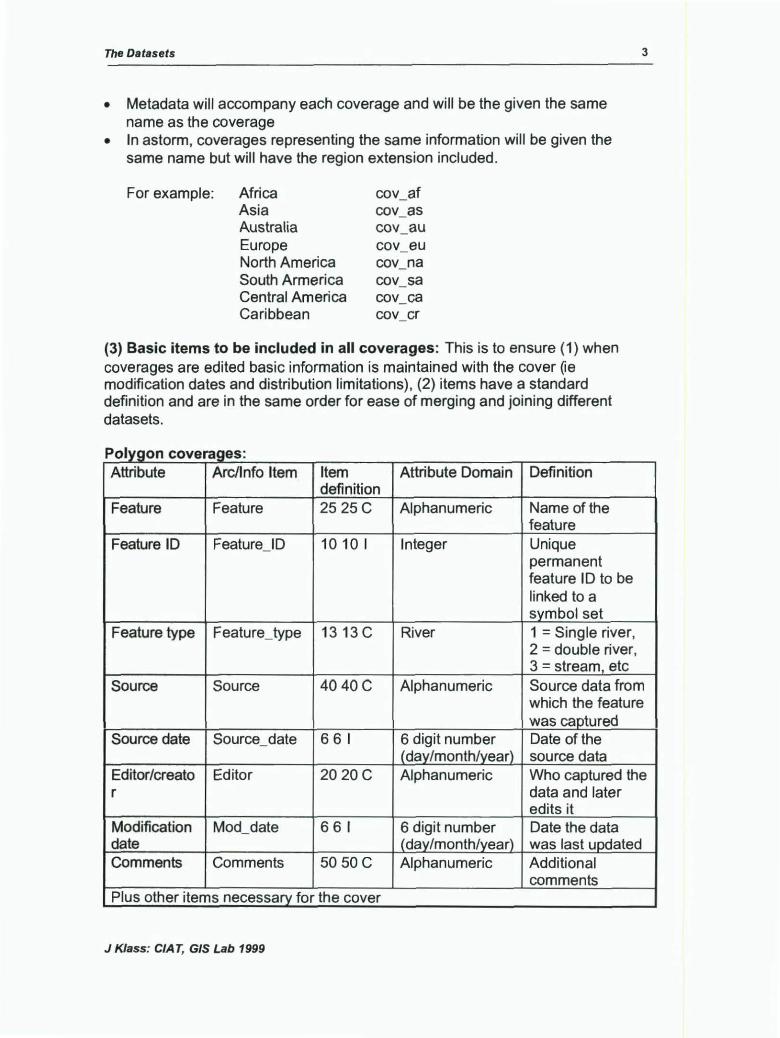
(3) Basic items to be included in all coverages: This is to ensure (1) when coverages are edited basic information is maintained with the cover Oe modification dates and distribution limitations), (2) items have a standard definition and are in the same order for ease of merging and joining different datasets.

p 1 olygon coverages: Attribute Arc/Jnfo ltem ltem Attribute Domain Definition

definition Feature Feature 25 25C Alphanumeric Name ofthe

feature Feature ID Feature_ ID 10 10 1 lnteger Unique

permanent feature 1 D to be linked toa symbol set

Feature type Feature_type 13 13 e River 1 = Single river, 2 = double river, 3 = stream etc

So urce So urce 4040C Alphanumeric Source data from which the feature was captured

Source date Source_date 661 6 digit number Date ofthe ( day/month/year) source data

Editor/creato Editor 2020C Alphanumeric Who captured the r data and later

edits it Modification Mod_date 661 6 digit number Date the data date ( day/month/year) was last updated Comments Comments 5050C Alphanumeric Additional

comments Plus other items necessary for the cover

J Klass: CIAT, GIS Lab 1999

The Dataseis 4

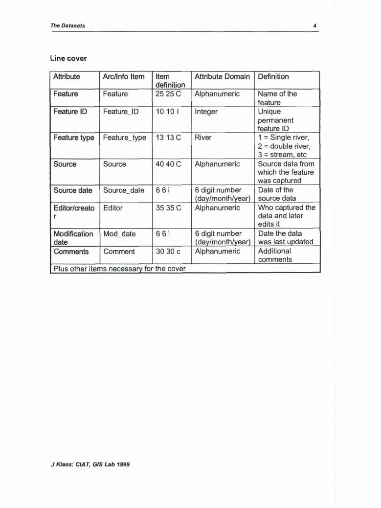
Line cover

Attribute Arcllnfo ltem ltem Attribute Domain Definition definition

Feature Feature 2525C Alphanumeric Name ofthe feature

Feature ID Feature_ID 10 10 1 lnteger Unique permanent feature ID

Feature type Feature_type 13 13 e River 1 = Single river, 2 = double river, 3 = stream, etc

So urce So urce 4040C Alphanumeric Source data from which the feature was capturad

Source date Source_date 6 6 i 6 digit number Date of the ( dav/month/vear) source data

Editor/creato Editor 35 35C Alphanumeric Who capturad the r data and later

edits it Modification Mod_date 66i 6 digit number Date the data date ( dav/month/vear) was last updated Comments Comment 30 30 e Alphanumeric Additional

comments Plus other items necessarv for the cover

J Klass: CIA T, GIS Lab 1999

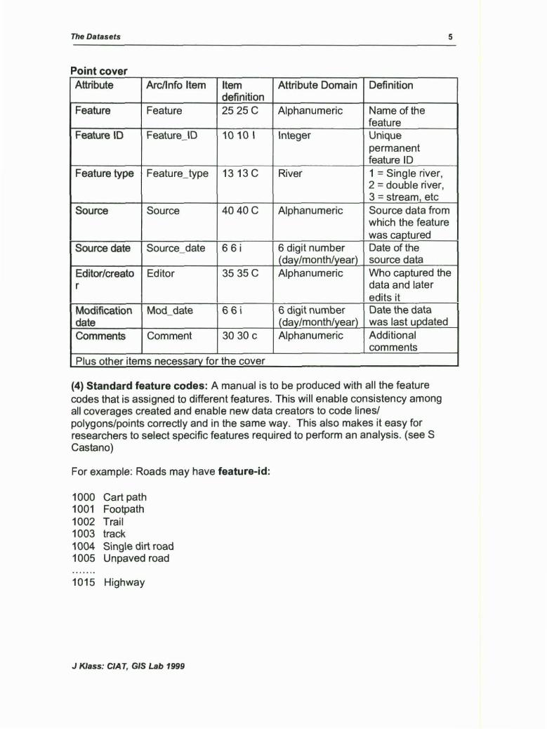
The Datasets 5

Point cover Attribute Arcllnfo ltem ltem Attribute Domain Definition

definition Feature Feature 2525C Alphanumeric Name ofthe

feature Feature ID Feature_lD 10 10 1 lnteger U ni que

permanent feature ID

Feature type Feature_type 1313C River 1 = Single river, 2 = double river, 3 = stream, etc

So urce So urce 4040C Alphanumeric Source data from which the feature was caotured

Source date Source_date 6 6 i 6 digit number Date ofthe ( dav/month/year) source data

Editor/creato Editor 35 35C Alphanumeric Who captured the r data and later

edits it Modification Mod_date 66i 6 digit number Date the data date {da y /month/vear) was last uodated Comments Comment 30 30 e Alphanumeric Additional

comments Plus other items necessarv for the cover

(4) Standard feature codes: A manual is to be produced with all the feature codes that is assigned to different features. This will enable consistency among all coverages created and enable new data creators to code lines/ polygons/points correctly and in the same way. This also makes it easy for researchers to select specific features required to perform an analysis. (see S Castano)

For example: Roads may have feature-id:

1 000 Cart path 1001 Footpath 1002 Trail 1003 track 1004 Single dirt road 1 005 Unpaved road

1015 Highway

J Klass: CJAT, GIS Lab 1999

The Datasets 6

(5) Data Dictionary of Coverages: A data dictionary is a document that contains the definition of a feature code (as illustrated in point (4)). This enables future users to identify the features in the coverage or grid. This is especially important for grids since these are numeric.

(6) Archive data and projects: A problem in the past has been the loss of data or poor archiving of completed projects and data. A directory has been setup on astorm for completed projects (/raid2/geodata/projects). When a project is completad it should be properly documented, archivad and stored where it will be available to all persons within the lab. This will be read only so new edits will not possible.

Accompanying these projects users should include: - metadata records (using Metalite), detailed documentation on how the data was created and in the case of applications a user's manual. The completad project will be written to CORO M and submitted to theGIS library, CIAT library (if necessary) to enable easy access to the information.

(7) Tools to access the data and search for data Three sets of tools can be u sed to search the data available in the GIS lab. These include: (a) Arcview Extension (J Klass, 1999 - created to access the digital data), (b) Web search http://gis.ciat.cgiar.org/ESRI (J Klass, 1997 with web programming by A Nelson), and (e) Documentation of Metalite on gisserver (J Klass, 1999).

Digital data at CIAT include the data created at the GIS lab at CIAT, information downloaded from the internet and through the collaboration of various institutes throughout Central America and the Caribbean.

All the data sets were processed using Arc/INFO 7.1 on a UNIX workstation.


The Datasets

Data lnfonnation

The data used in this analysis were collected from various sources, including surveys and creating data layers by the digitizing team, past and present students, senior scientists and researchers at CIA T. All the data has been processed in the GIS lab at CIAT using a ran~e of available GIS and remote sensing software. These include Arc/lnfo ESR, Arcview3 GIS ESRI, PCI, Imagine Erdas and ldrisi Clark University .

The information used in the whitefly study included;

• Data obtained via the intemet from si tes such as the USGS

• National agricultura! censuses

• CIA T's climate data base

• Personal communications from national program staff visiting CIAT

7

• Personal communícation with national program staff in ea eh of the study sites

The source of each data set is briefly discussed with a more detailed explanation of the steps taken in the development of coverages/surfaces, also known as themes or layers, to be used in the analysis. The data included the creation of environmental data (includes climate surfaces), the location of crops and location of whitefly transmitted gemini-viruses.

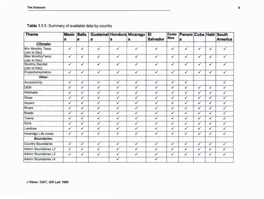
The data that has been collected and induded on the cdrom has been summarized in Table 1.1.1. Table 1.1.1 summarizes, by country, the data that was available at the time. The table highlights areas where data is missing and can aid in developing future data collection strategies.

J K/ass: C/A T, GIS Lab 1999

The Datasets 8

Table 1.1.1 : Summary of available data by country

Theme Mexic Beliz Guatemal Hondura Nlcaragu El Coabl Pana m Cuba Halti South o • a • a Salvador Rica a Ame rica

Climate: Min Monthly Temp ./ ./ ./ ./ ./ ./ ./ ./ ./ ./ ./ (Jan to Dec) Max MonthlyTemp

[{Jan to Dec) ./ ./ ./ ./ ./ ./ ./ ./ ./ ./ ./

Monthly Rainfall ./ ./ ./ ./ ./ ./ ./ ./ ./ ./ ./ I<Jan to Dec) Evapotranspiration ./ ./ ./ ./ ./ ./ ./ ./ ./ ./ ./

Other:

Accessibility ./ ./ ./ ./ ./ ./ ./ ./ ./

DEM ./ ./ ./ ./ ./ ./ ./ ./ ./ ./ ./

Hillshade ./ ./ ./ ./ ./ ./ ./ ./ ./ ./ ./

Slope ./ ./ ./ ./ ./ ./ ./ ./ ./ ./ ./

Aspect ./ ./ ./ ./ ./ ./ ./ ./ ./ ./ ./

Rivers ./ ./ ./ ./ ./ ./ ./ ./ ./ ./ ./ Roads ./ ./ ./ ./ ./ ./ ./ ./ ./ ./ ./

Towns ./ ./ ./ ./ ./ ./ ./ ./ ./ ./ ./

Soils ./ ./ ./ ./ ./ ./ ./ ./ ./ ./ ./

Landuse ./ ./ ./ ./ ./ ./ ./ ./ ./ ./ ./

Holdridge Lite zonas ./ ./ ./ ./ ./ ./ ./ ./ ./ ./ ./ Boundartes:

Country Boundaries ./ ./ ./ ./ ./ ./ ./ ./ ./ ./ ./

Admin Boundaries L2 ./ ./ ./ ./ ./ ./ ./ ./ ./ ./ ./

Admin Boundaries L3 ./ ./ ./ ./ ./ ./ ./ ./ ./ ./ ./

Admin Boundaries L4 ./ ./


The Datasets 9

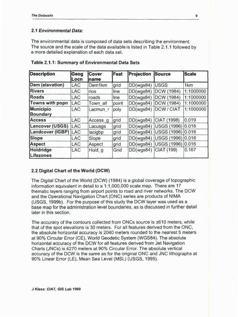
2.1 Environmental Data:

The environmental data is composed of data sets describing the environment. The source and the scale of the data available is listed in Table 2.1.1 followed by a more detailed explanation of each data set.

Table 2.1.1: Summary of Environmental Data Sets

Description Geog Cover Feat Projection Source Sea le llocn na me

Dem (elevation) LAC Dem1km grid DD(wgs84) USGS 1km Rivers LAC ríos line DD(wgs84) DCW-(1984) 1:1000000 Roads LAC roads line DD(wgs84) DCW (1984) 1:1000000 Towns with popn LAC Town all point DD(wgs84) DCW (1984) 1:1000000 Municipio LAC Lacmun_r poi y DD(wgs84) DCW / CIAT 1:1000000 Boundary Access LAC Access _g ,grid DD(wgs84) CIAT(1998) 0.019 Lancover (USGS) LAC Lacusgs lgrid DD(wgs84) USGS (1996) 0.016 Landcover (IGBP) LAC lacigbp lgrid DD(wgs84) USGS(1996) 0.016 Slope LAC Slope lgrid DD(wgs84) USGS (1996) 0.016 Aspect LAC Aspect lgrid DD(wgs84) USGS (1996) 0.016 Holdridge LAC Hold_g Grid DD(wgs84) CIAT (199) 0.167 Lifezones

2.2 Digital Chart of the Wortd (DCW)

The Digital Chart of the World (DCW) ( 1984) is a global coverage of topographic information equivalent in detail to a 1:1 ,000,000 scale map. There are 17 thematic layers ranging from airport points to road and river networks. The DCW and the Operational Navigation Chart (ONC) series are products of NIMA (USGS, 1999b). For the purpose of this study the DCW layer was used as a base map for the administration level boundaries, as is discussed in turther detail later in this section.

The accuracy of the contours collected from ONCs source is ±610 meters, while that of the spot elevations is 30 meters. For all features derived from the ONC, the absoluta horizontal accuracy is 2040 meters rounded to the nearest 5 meters at 90% Circular Error (CE), World Geodetic System (WGS84). The absoluta horizontal accuracy of the DCW for all features derivad from Jet Navigation Charts (JNCs) is 4270 meters at 90% Circular Error. The absoluta vertical accuracy of the DCW is the same as for the original ONC and JNC lithographs at 90% Linear Error (LE), Mean Sea Level (MSL) (USGS, 1995).


The Datasets 10

2.3 USGS Digital Elevation Model (DEM)

The DEM was developed by the U.S. Geological Survey's EROS Data Center, Sioux Falls, South Dakota, 1996. The elevations are regularly spaced at 30-arc seconds (0.008333333 degrees), approximately 1 kilometer (USGS, 1997). The DEM was derived from eight data sources, both vector and raster. These include the digital terrain elevation data (DTED) with a horizontal grid spacing of 3-arc seconds (90 meters), digital chart of the world (DCW), the USGS 1 -degree DEM's, Army map Service (AMS) 1:1 ,000,000-scale maps and the lnternational map of the world (IMW) 1:1 ,000,000-scale map. For Central America the main sources used was from the DTED with enhancements made by the DCW data (USGS, 1999b; USGS, 1997).

Of the DCW data, the hypsography and drainage layers were the most applicable to be included in the DEM generation, since these contain topographic information. For elevations below 305 metres, the primary contour interval on the source ONC's is 305 meters with supplemental contours at 76 meters intervals. For higher elevations the supplemental contours are at 152-meter intervals. The DTED and USGS DEM's have a vertical accuracy of + or- 30 meters linear error at the 90 percent confidence level (USGS, 1997).

Refer to: dem1 km, hillshade, slope, aspect

Hillshade: A shaded relief was created in arc/info using the hillshade command using dem1km.

Slope: The slope surface was created in arc/info using the slope command using dem1km.

Aspect: The aspect grid was created in arc/info using the aspect command using dem1km.

2.4 USGS Land Cover

The U.S. Geological Survey (USGS), the University of Nebraska-Lincoln (UNL), and the European Commission's Joint Research Centre (JRC) generated a 1-km resolution global land cover databa se. The land cover was developed on a continent-by-continent basis with a 1-km nominal spatial resolution, based upon 1-km Advanced Very High-Resolution Radiometer (AVHRR) data from April 1992 through March 1993. The finalland cover is composed of several data sources; AVHRR Data, Digital Elevation Model (DEM) Data, Ecoregions Data and Map Data (USGS, 1999c).

The finalland cover was determinad using a 'convergence of evidence approach' which used three interpreters to insure consistency. This included the seasonal land cover regions as defined by the Global Ecosystem framework which were


The Datasets 11

cross-reference to the land cover classes of the Simple Biosphere Model (SIB), Simple Biosphere 2 Model, the Biosphere Atmosphere Transfer Scheme (BATS), lnternational Geosphere Biosphere Programme (IGBP), and the USGS/Anderson (USGS, 1999c).

The final task associated with this step is the generation of the derivad data sets,including land cover and seasonal measures. In this step, the seasonal land cover regions are aggregated (or renumbered) into the appropriate classes of the output classification legends. Urban areas, extractad from the Digital Chart of the World (Defensa Mapping Agency, 1992) are added to three of the derivad data sets: Global Ecosystems, IGBP Land Cover, and the USGS Land Use/Land Cover system.

Refer to: Lacusgs, lacigbp

2.5 Accessibility

The accessibility surface was created at CIAT by A. Nelson (1998) using the following information and methodology. The accessibility model is a land based model and does not account for air travel , which may play an important role for more remote areas. The model al so ignores the transport of perishable goods that are often freighted by air. Coastal access by launch or ferry is also ignore d. The projection used to create the surta ces was Lambert equal area azimuthal.

The model is based on the cost distance function in are /info which requires a point based grid for source locations anda friction surface which defines the ease with which each cell can be traversed. The influencing factors which composed the friction surface include: -roads, rail, navigable rivers, slope, land cover, urban areas

The data sources included: (roacts (DCW); rail (DCW); rivers (DCW); slope (GTOP030: http://edcwww.cr.usgs.gov/landdaac/gtopo30/gtopo30.html); land cover (IGBP:http://edcwww.cr.usgs.gov/landdaac/glcc/glcc.html); urban areas ( NOAA:http:/ /www .ngdc.noaa.gov:8080/production/htmVbiomass/night. html))

Each of these is in the form of a 1 km resolution grid that is classified to describe it's contribution to the friction surface. The factors were combinad in arc/info to create a friction surface.

Refer to: access_g

Reference: ftp://geog.leeds.ac.uk/pub/andynelson/accessibilitv.doc

Or /raid2/geodata/data_info/accessibility.pdf


The Dataseis 12

2.6 Climate data information

The CIAT climate surfaces were developed by P Jones at CIAT, and are based on 30 year climate averages from about 10,000 stations in Latin America (Jones et al. 1999). The surfaces were interpolated using 'the inverse square of the distance between the five nearest stations and the interpolated point'. The temperatura surfaces were 'standardized to the elevation of the pixel in the DEM using a lapse rate model' (Jones et al. 1999). The surfaces were include the following;


The Datasets 13

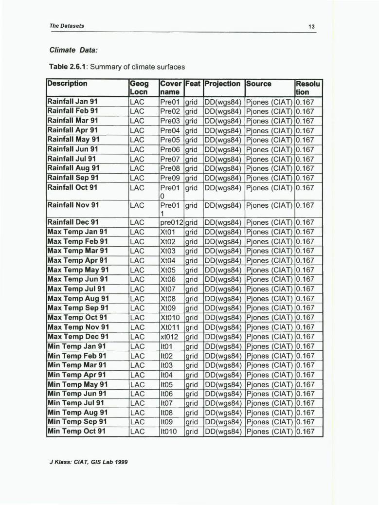
Climate Data:

Table 2.6.1 : Summary of clima te surta ces

Description Geog Cover Feat Projection Source Resol u Loen na me tlon

Rainfall Jan 91 LAC Pre01 ¡grid DD(wgs84)_ Pjones (CIA T) 0.167 Rainfall Feb 91 LAC Pre02 grid DD(wgs84) Pjones (CIAT) 0.167 Rainfall Mar 91 LAC Pre03 ¡grid DD(wgs84) Pjones (CIAT) 0.167 Rainfall Apr 91 LAC Pre04 ¡grid DD(wgs84) Pjones (CIAT) 0.167 Rainfall May 91 LAC Pre05 grid DD(wgs84) Pjones (CIA T) 0.167 Rainfall Jun 91 LAC Pre06 grid DD(w_gs84) Pjones (CIA T) 0.167 Rainfall Jul91 LAC Pre07 ¡grid DD(wgs84}_ Pjones _iCI/ill_ 0.167 Rainfall Aug 91 LAC Pre08 grid DD(wgs84) Pjones (CIA T) 0.167 Rainfall Sep 91 LAC Pre09 ¡grid DD(wgs84) Pjones (CIAT) 0.167 Rainfall Oct 91 LAC Pre01 grid DD(wgs84) Pjones (CIAT) 0.167

o Rainfall Nov 91 LAC Pre01 grid DD(wgs84) Pjones (CIAT) 0.167

1 Rainfall Dec 91 LAC pre012 grid DD(wgs84) Pjones (CIA T) 0.167 Max Temp Jan 91 LAC Xt01 ¡grid DD(wgs841 Pjones _iCIA_TI_ 0.167 Max Temp Feb 91 LAC Xt02 ¡grid DDJwgs84l Pjones JCIA_!}_ 0.167 Max Temp Mar 91 LAC Xt03 grid DD(wgs84) Pjones (CIAT) 0.167 Max Temp Apr 91 LAC Xt04 ¡grid DD(wgs84}_ Pjones JCIATl 0.167 Max Temp May 91 LAC Xt05 l_grid DD(wgs84) Pjones (CIAT) 0.167 Max Temp Jun 91 LAC Xt06 grid DD(wgs84) Pjones (CIA T) 0.167 Max Temp Jul 91 LAC Xt07 ¡grid DD(wgs84}_ Pjones JCIA _TI_ 0.167 Max Temp Aug 91 LAC X tOS lg_rid DD_{w_g_s84) Pjones (CIAT) 0.167 Max Temp Sep 91 LAC Xt09 grid DD(wgs84) Pjones (CIA T) 0.167 Max Temp Oct 91 LAC Xt010 grid DD(wgs84}_ Plones JCI/ill_ 0.167 Max Temp Nov 91 LAC Xt011 grid DD(wgs84l Plones l_CIA T) 0.167 Max Temp Dec 91 LAC xt012 grid DD(wgs84) Pjones (CIAT) 0.167 Min Temp Jan 91 LAC lt01 grid DD(wgs84)_ Pjones _iCIA_!)_ 0.167 Min Temp Feb 91 LAC lt02 grid DD_iw_g_s84l Plones l_CI'ill_ 0.167 Min Temp Mar 91 LAC lt03 grid DD(wgs84) Pjones (CIAT) 0.167 Min Temp Apr 91 LAC lt04 grid DD(wgs84) Pjones (CIAT) 0.167 Min Temp May 91 LAC lt05 grid DD(wgs84l Pjones _{CIAD_ 0.167 Min Temp Jun 91 LAC lt06 grid DD(wgs84) Pjones (CIAT) 0.167 Min Temp Jul 91 LAC lt07 lg_rid DD_iw_g_s84l Pjones JCIA __!)__ 0.167 Min Temp Aug 91 LAC lt08 ¡grid DD(wgs84) Pjones (CIA T) 0.167 Min Temp Sep 91 LAC lt09 grid DD(wgs84) Pjones (CIA T) 0.167 Min Temp Oct 91 LAC lt010 grid DD(wgs84) Pjones (CIAT) 0.167

J K/ass: CIAT, GIS Lab 1999

The Datasets 14

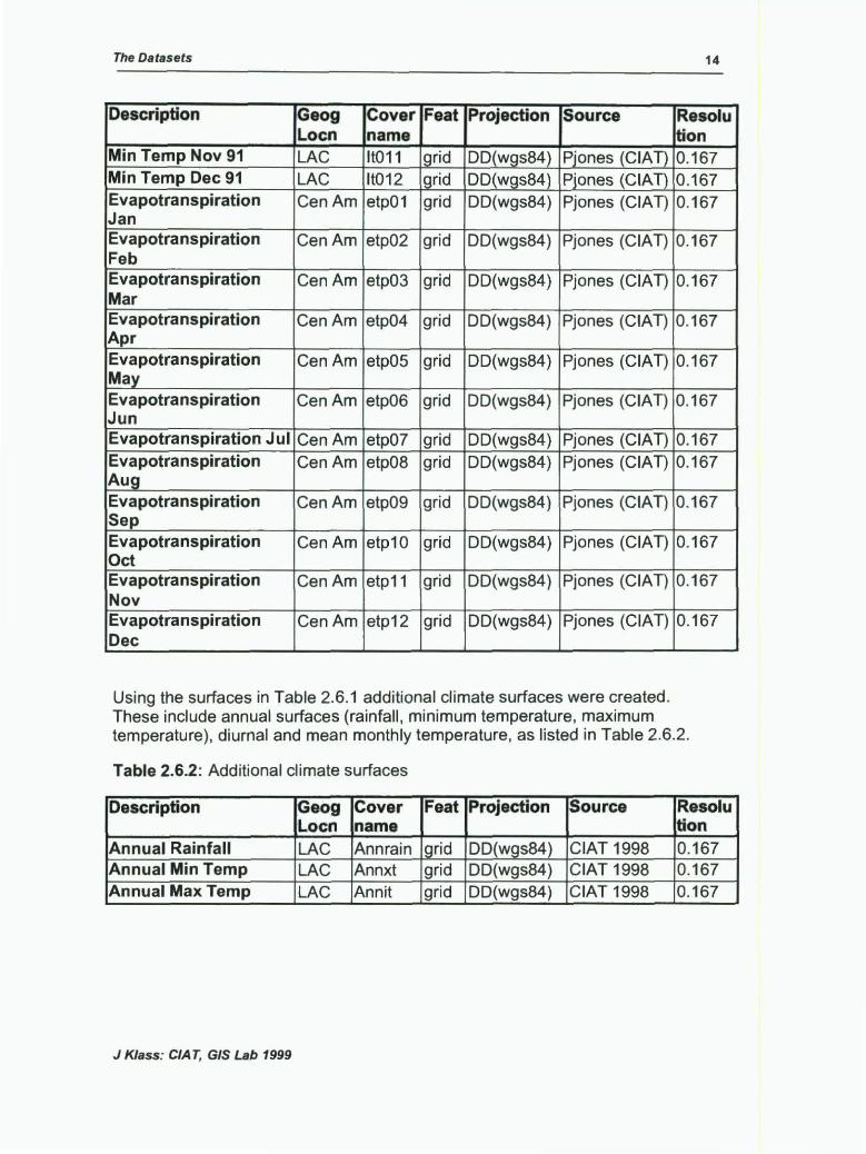
Description Geog Cover Feat Projaction So urca Resol u Loen na me tion

Min Temp Nov 91 LAC lt011 [grid DD(wgs84) Pjones (CIAT) 0.1 67 Min Temp Dec 91 LAC lt012 [grid DDiw_g_s84) Piones (CIA]) 0.167 Evapotranspiration CenAm etp01 Jan

grid DD(wgs84) Pjones (CJAT) 0.167

Evapotranspiration CenAm etp02 grid DD(wgs84) Pjones (CIA T) 0.167 Feb Evapotranspiration CenAm etp03 grid DD(wgs84) Pjones (CJAT) 0.167 Mar Evapotranspiration CenAm etp04 grid DD(wgs84) Pjones (CIA T) 0.167 Apr Evapotranspiration CenAm etp05 grid DD(wgs84) Pjones (CIA T) 0.167 M a _y Evapotranspiration CenAm etp06 grid DD(wgs84) Pjones (CJAT) 0.167 Jun Evapotranspiration Jul CenAm etp07 grid DD(wgs84) Pjones (CIA T) 0.167 Evapotranspiration CenAm etp08 grid DD(wgs84) Pjones (CIA T) 0.167 Aug Evapotranspiration CenAm etp09 grid DD(wgs84) Pjones (CIAT) 0.167 Sep Evapotranspiration CenAm etp10 grid DD(wgs84) Pjones (CIAT) 0.167 Oct Evapotranspiration CenAm etp11 grid DD(wgs84} Pjones (CIA T) 0.167 Nov Evapotranspiration CenAm etp12 grid DD(wgs84) Pjones (CIA T) 0.167 De e

Using the surfaces in Table 2.6.1 additional climate surfaces were created. These include annual surfaces (rainfall , mínimum temperature, maximum temperatura), diurna! and mean monthly temperatura, as listed in Table 2.6.2.

Table 2.6.2: Additional climate surfaces

Description Geog Covar Feat Projection Source Resol u Loen nama ltion

Annual Rainfall LAC Annrain 'grid DD(wgs84) CJAT 1998 0.167 Annual Min Temp LAC Annxt grid DD(wgs84) CJAT 1998 0.167 Annual Max Temp LAC Annit grid DD(wgs84) CIAT 1998 0.167

J K/ass: C/A T, G/S Lab 1999

The Datasets 15

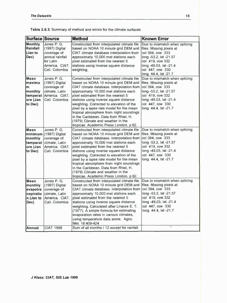
Table 2.6.3: Summary of method and errors for the climate surfaces

Surface Source Method Known Error Monthly Jones P. G. Constructed from lnterpolated climate file Due to mismatch when splicing Ralnfall ( 1997) Digital based on NOAA 1 O minute grid DEM and files. Mlssing pixels at (Jan to coverage ot CIAT climate database lnterpolation from col 394, row 333 Dec) annual rainfall approximatly 10,000 met stations each long -53.2, lat -21 .57

for Latin pixel estimated from the nearest 5 col 419, row 332 America. CIAT. stations using lnverse square distance long -49.03. lat -21.4 Cali. Colombia weighting. col 447, row 330

Ion¡:¡ 44.4, lat -21.7 Mean Jones P. G. Constructed from interpolated climate file Dueto mismatch when splicing maxlmu (1997) Digital based on NOAA 1 O minute grid DEM and files. Missing pixels at m coverage of CIAT climate database. lnterpolation from col 394, row 333 monthly climate, Latin approximatly 10,000 met stations each long -53.2, lat -21.57 temperat America. CIAT. pixel estimated from the nearest 5 col 419, row 332 ure (Jan Cali. Colombia stations using inverse square distance long -49.03, lat -21.4 to Dec) weighting. Corrected to elevation of the col 447, row 330

pixel by a lapse rate model for the mean long 44.4, lat -21 .7 tropical atmosphere from night soundings in the Caribbean. Data from Rhiel, H. (1979) Climate and weather in the tropicas. Academic Press London. p 62.

Mean Jones P. G. Constructed from interpolated climate file Due to mismatch when splicing minlmum ( 1997) Digital based on NOAA 1 O minute grid DEM and files. Missing pixels at monthly coverage of CIAT climate database. lnterpolation from col 394, row 333 temperat climate, Latin approximatly 10,000 met stations each long -53.2, lat -21.57 ure (Jan America. CIAT. pixel estimated from the nearest 5 col 419, row 332 to Dec) Cali. Colombia stations using inverse square distance long -49.03, lat -21.4

weighting. Corrected to elevation of the col 447, row 330 pixel by a lapse rate model for the mean long 44.4, lat -21 .7 tropical atmosphere from night soundings in the Caribbean. Data from Rhiel, H. (1979) Climate and weather in the tropicas. Academic Press London. p 62.

Mean Jones P. G. Constructed from interpolated climate file Due to mismatch when splicing monthly (1997) Digital based on NOAA 1 O minute grid DEM and files. Missing pixels at evapotra coverage of CIAT climate database. lnterpolation from col 394, row 333 nsplratlo climate, Latín approximatly 10,000 met stations each long -53.2, lat -21 .57 n (Jan to America. CIA T. pixel estimated from the nearest 5 col 419. row 332 Dec) Cali. Colombia stations using inverse square distance long -49.03 , lat -21 .4

weighting. Calculated after Llnacre E. T. col 447, row 330 (1977). A simple formula for estimating long 44.4, lat -21 .7 evaporation rates in various climates, using temperatura data alone. Agric. Met. 18:409-424

Annual CIAT 1998 Sum of all months /12 except for rainfall "

J KJass: CIAT, GIS Lab 1999

The Datasets

2. 7 Holdridge LifeZones

Constructed from interpolated climate file based on NOAA 1 O minute grid DEM and CIAT climate database. lnterpolation from approximately 10,000 met stations each estimated from the nearest 5 stations using inverse square distance weighting. The Holdridge classifications were defined by Holdridge, (1967).

Refer to: hold_g

Reference: Jones P. G. (1998) Holdridge lite Zones ot Latín America, Digital image. CIAT. Cali. Colombia

Holdridge, L.R. , 1967. Lite zone ecology. Tropical Science Center, San Jose, Costa Rica

2.8 CIAT's Administration Boundary Coverage

16

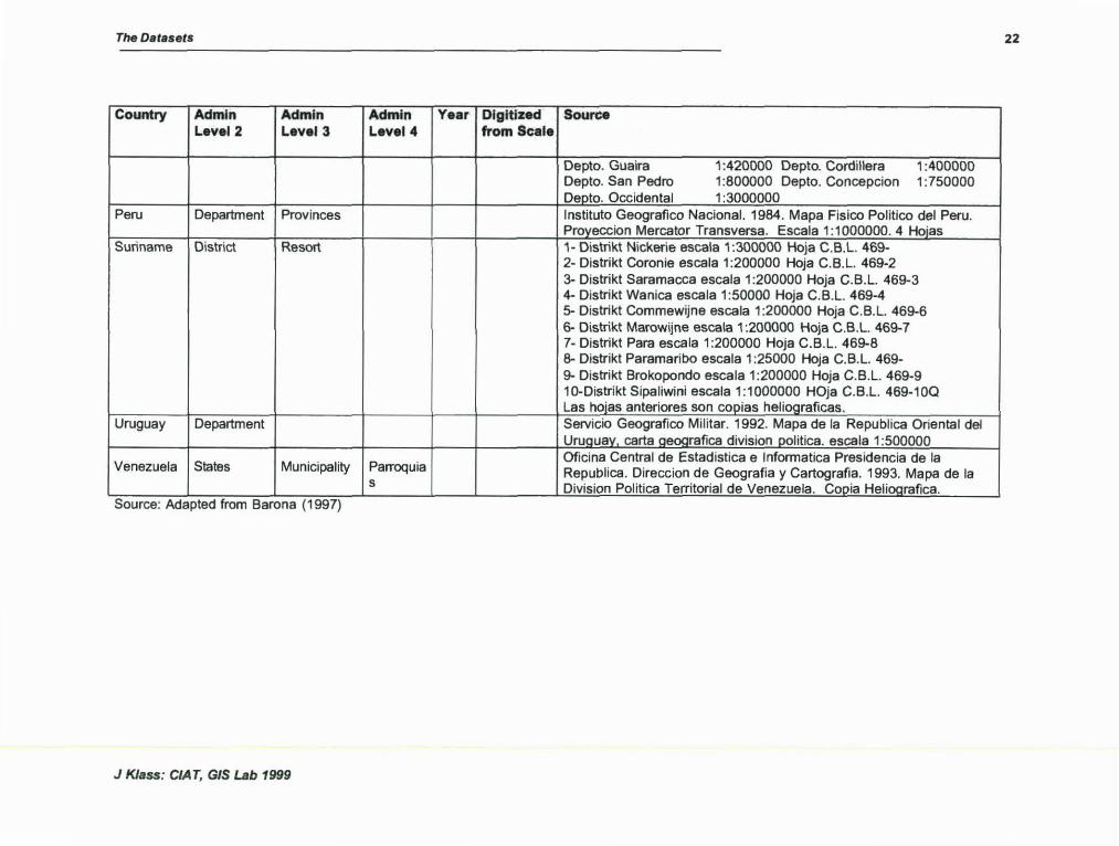
The information contained in the administration boundary coverage was digitized in the GIS lab at CIAT in 1996. The boundarias wara digitized country by country and adjusted to the OCW (Digital Chart of tha World) country boundary. Tha lnformation contained in tha covaraga includes thraa admlnistration boundary levals; the country boundary, province or department and municlpalities. The boundary lnformation was obtained from maps of various scales, as listad In Tabla 2.9.1 (Barona, 1997).

Refer to: adm_lac

Jones, P. G. and Bell, W. C. (1997) Coverage of Latin America Administrativa Olvisions. Version 1.1 Apr 1997 digital dataset. CIAT Cali Colombia


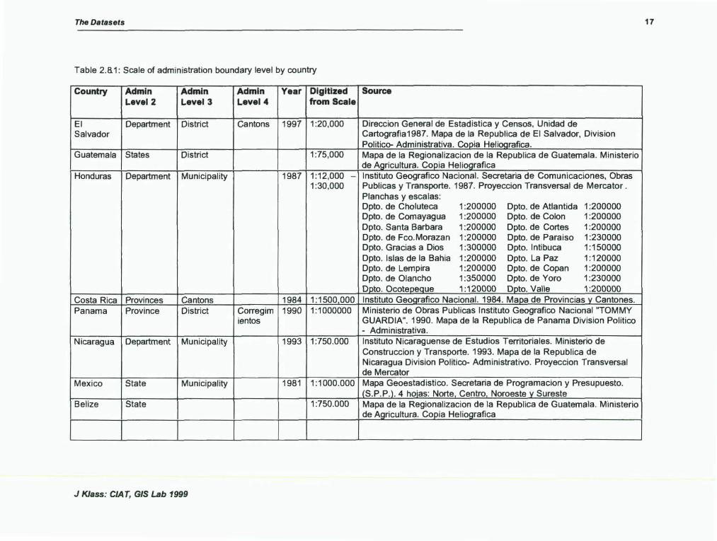
The Dataseis 17

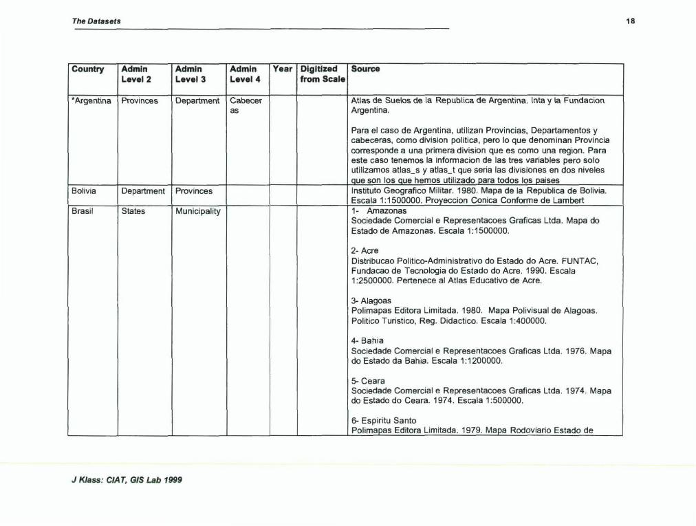
Table 2.81 : Scale of administration boundary level by country

Country Admln Admln Admln Year Dlgltlzed Source Level2 Level3 Level4 from Scale

El Department District Cantons 1997 1:20,000 Direccion General de Estadistica y Censos, Unidad de Salvador Cartografia1987. Mapa de la Republica de El Salvador, Division

Politico- Administrativa. CoQia Heliografica. Guatemala S tates District 1:75,000 Mapa de la Regionalizacion de la Republica de Guatemala. Ministerio

de Agricultura. Copia Heliografica Honduras Department Municipality 1987 1:12,000 - Instituto Geografico Nacional. Secretaria de Comunicaciones, Obras

1:30,000 Publicas y Transporte. 1987. Proyeccion Transversal de Mercator . Planchas y escalas: Opto. de Choluteca 1:200000 Opto. de Atlantida 1:200000 Opto. de Comayagua 1:200000 Opto. de Colon 1:200000 Opto. Santa Barbara 1:200000 Opto. de Cortes 1:200000 Opto. de Fco.Morazan 1:200000 Opto. de Paraiso 1:230000 Opto. Gracias a Dios 1:300000 Opto. lntibuca 1:150000 Opto. Islas de la Bahia 1:200000 Opto. La Paz 1:120000 Opto. de Lempira 1:200000 Opto. de Copan 1:200000 Opto. de Olancho 1:350000 Opto. de Yoro 1:230000 Opto. Ocotep_egue 1:120000 Opto. Valle 1:200000

Costa Rica Provinces Cantons 1984 1:1500 000 Instituto Geoorafico Nacional. 1984. Maoa de Provincias v Cantones. Panama Province District Corregim 1990 1:1000000 Ministerio de Obras Publicas Instituto Geografico Nacional ''TOMMY

ientos GUARDIA". 1990. Mapa de la Republica de Panama Division Politico - Administrativa.

Nicaragua Department Municipality 1993 1:750.000 Instituto Nicaraguense de Estudios Territoriales. Ministerio de Construccion y Transporte. 1993. Mapa de la Republica de Nicaragua Division Politico- Administrativo. Proyeccion Transversal de Mercator

Mexico S tate Municipality 1981 1:1000.000 Mapa Geoestadistico. Secretaria de Programacion y Presupuesto. (S.P.P.). 4 hoias: Norte Centro Noroeste v Sureste

Belize State 1:750.000 Mapa de la Regionalizacion de la Republica de Guatemala. Ministerio de Agricultura. Copia Heliografica


The Datasets 18

Countty Admln Admln Admln Year Dlgltlzed Source Level2 Level3 Level4 from Scale

*Argentina Provinces Department Cabecer Atlas de Suelos de la Republica de Argentina. lnta y la Fundacion as Argentina.

Para el caso de Argentina, utilizan Provincias, Departamentos y cabeceras, como division política, pero lo que denominan Provincia corresponde a una primera division que es como una region. Para este caso tenemos la informacion de las tres variables pero solo utilizamos atlas_s y atlas_t que seria las divisiones en dos niveles aue son los aue hemos utilizado para todos los paises

Bolivia Department Provinces Instituto Geografico Militar. 1980. Mapa de la Republica de Bolivia. Escala 1:1500000. Pro_y_eccion Canica Conforme de Lambert

Brasil S tates Municipality 1- Amazonas Sociedade Comercial e Representacoes Graficas Ltda. Mapa do Estado de Amazonas. Escala 1:1500000.

2- Acre Distribucao Político-Administrativo do Estado do Acre. FUNTAC, Fundacao de Tecnología do Estado do Acre. 1990. Escala 1 :2500000. Pertenece al Atlas Educativo de Acre.

3- Alagoas Polimapas Editora Limitada. 1980. Mapa Polivisual de Alagoas. Politico Turistico, Reg. Didactico. Escala 1 :400000.

4- Bahia Sociedade Comercial e Representacoes Graficas Ltda. 1976. Mapa do Estado da Bahia. Escala 1:1200000.

5- Ceara Sociedade Comercial e Representacoes Graficas Ltda. 1974. Mapa do Estado do Ceara. 197 4. Escala 1 :500000.

6- Espiritu Santo Polima_j)_as Editora Limitada. 1979. Mapa Rodoviario Estado de


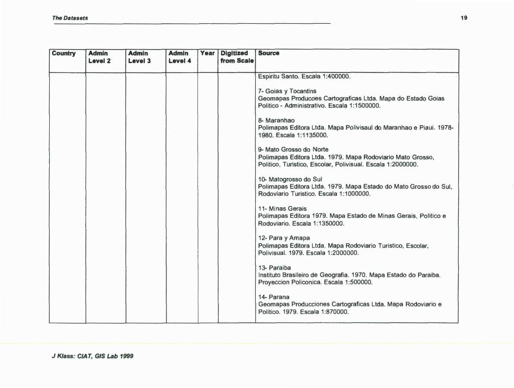
The Oatasets 19

Country AdmJn Admln Admln Year Dlgltiud Source Level2 Level3 Level4 fr'om Scale

Espiritu Santo. Escala 1:400000.

7- Goias y Tocantins Geomapas Producoes Cartograficas Ltda. Mapa do Estado Goias Politico- Administrativo. Escala 1:1500000.

8- Maranhao Polimapas Editora Ltda. Mapa Polivisaul do Maranhao e Piaui. 1978-1980. Escala 1:1135000.

9- Mato Grosso do Norte Polimapas Editora Ltda. 1979. Mapa Rodoviario Mato Grosso, Politico, Turistico, Escolar, Polivisual. Escala 1 :2000000.

10- Matogrosso do Sul Polimapas Editora Ltda. 1979. Mapa Estado do Mato Gros so do Sul, Rodoviario Turistico. Escala 1:1000000.

11- Minas Gerais Polimapas Editora 1979. Mapa Estado de Minas Gerais, Político e Rodoviario. Escala 1:1350000.

12- Para y Amapa Polimapas Editora Ltda. Mapa Rodoviario Turistico, Escolar, Polivisual. 1979. Escala 1:2000000.

13- Paraiba Instituto Brasileiro de Geografía. 1970. Mapa Estado do Paraiba. Proyeccion Policonica. Escala 1 :500000.

14- Parana Geomapas Producciones Cartograficas Ltda. Mapa Rodoviario e Politico. 1979. Escala 1 :870000.

J K/ass: CIAT, GIS Lab 1999

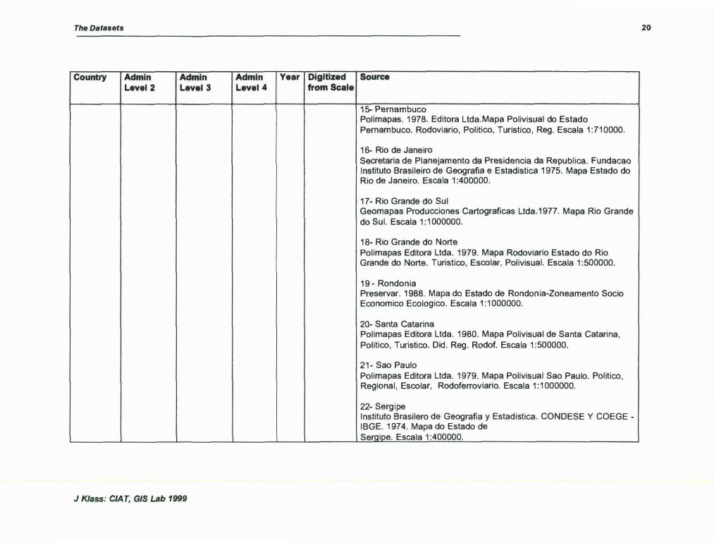
The Datasets 20

Country Admln Admln Admln Year Dlgltized Source Level2 Level3 Level4 from Scale

1 ~ Pernambuco Polimapas. 1978. Editora Ltda.Mapa Polivisual do Estado Pernambuco. Rodoviario, Político, Turístico, Reg. Escala 1:710000.

16- Rio de Janeiro Secretaria de Planejamento da Presidencia da Repubtica. Fundacao Instituto Brasileiro de Geografia e Estadistica 1975. Mapa Estado do Rio de Janeiro. Escala 1:400000.

17- Rio Grande do Sul Geomapas Producciones Cartograflcas Ltda.1977. Mapa Rio Grande do Sul. Escala 1:1000000.

18- Rio Grande do Norte Polimapas Editora Ltda. 1979. Mapa Rodoviario Estado do Río Grande do Norte. Turístico, Escolar, Polivisual. Escala 1 :500000.

19 - Rondonia Preservar. 1988. Mapa do Estado de Rondonia-Zoneamento Socio Economico Ecologico. Escala 1:1000000.

20- Santa Catarina Polimapas Editora Ltda. 1980. Mapa Polivisual de Santa Catarina , Político, Turístico. Did. Reg. Rodof. Escala 1:500000.

21 - Sao Paulo Polimapas Editora Ltda. 1979. Mapa Polivisual Sao Paulo. Político, Regional, Escolar, Rodoferroviario. Escala 1:1 000000.

22- Sergipe Instituto Brasilero de Geografla y Estadistica. CONDESE Y COEGE -IBGE. 1974. Mapa do Estado de Seraioe. Escala 1:400000.

J KJass: CIA T, GIS Lab 1999

The Datasets 21

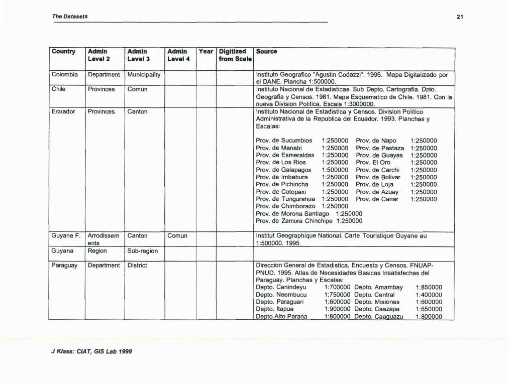
Country Admln Admln Admln Year Dlg_ltlzed Source Level2 Level3 Level4 from Scafe

Colombia Department Municipality Instituto Geografico M Agustín Codazzi". 1995. Mapa Digitalizado por el DANE. Plancha 1 :500000.

Chile Provinces Comun Instituto Nacional de Estadísticas. Sub Depto. Cartografía. Opto. Geografía y Censos. 1981. Mapa Esquematico de Chile. 1981. Con la nueva Division Política. Escala 1:3000000.

Ecuador Provinces Canton Instituto Nacional de Estadistica y Censos. Division Político Administrativa de la Republica del Ecuador. 1993. Planchas y Escalas:

Prov. de Sucumbios 1:250000 Prov. de Napo 1:250000 Prov. de Manabi 1:250000 Prov. de Pastaza 1:250000 Prov. de Esmeraldas 1:250000 Prov. de Guayas 1:250000 Prov. de Los Rios 1:250000 Prov. El Oro 1:250000 Prov. de Galapagos 1:500000 Prov. de Carchi 1:250000 Prov. de lmbabura 1:250000 Prov. de Bolívar 1:250000 Prov. de Pichincha 1:250000 Prov. de Loja 1:250000 Prov. de Cotopaxi 1:250000 Prov. de Azuay 1:250000 Prov. de Tungurahua 1:250000 Prov. de Canar 1:250000 Prov. de Chimborazo 1:250000 Prov. de Morona Santiago 1:250000 Prov. de Zamora Chinchipe 1 :250000

Guyane F. Arrodissem Canton Comun lnstitut Geographique National. Carte Touristique Guyane au ents 1 :500000. 1995.

Guyana Region Sub-region

Paraguay Department District Direccion General de Estadistica, Encuesta y Censos. FNUAP-PNUD. 1995. Atlas de Necesidades Basicas Insatisfechas del Paraguay. Planchas y Escalas: Depto. Canindeyu 1:700000 Depto. Amambay 1:850000 Depto. Neembucu 1:750000 Depto. Central 1:400000 Depto. Paraguari 1:600000 Depto. Misiones 1:600000 Depto. ltapua 1:900000 Depto. Caazapa 1:650000 Depto.Aito Parana 1:800000 Depto. Caaouazu 1:800000


The D•t.aets 22

Country Admln Admln Admln Year Dlgltlzed Source Level2 Level3 Level4 from Scale

Depto. Guaira 1:420000 Depto. Cordillera 1:400000 Depto. San Pedro 1:800000 Depto. Concepcion 1:750000 Deoto. Occidental 1:3000000

Peru Department Provinces Instituto Geografico Nacional. 1984. Mapa Físico Político del Peru. Proyeccion Mercator Transversa. Escala 1:1000000. 4 Hoias

Suriname District Resort 1- Distrikt Nickerie escala 1:300000 Hoja C. B. L. 469-2- Distrikt Coronie escala 1:200000 Hoja C.B.L. 469-2 3- Distrikt Saramacca escala 1:200000 Hoja C.B.L. 469-3 4- Distrikt Wanica escala 1:50000 Hoja C.B.L. 469-4 5- Distrikt Commewijne escala 1:200000 Hoja C.B.L. 469-6 ~ Distrilct Marowijne escala 1:200000 Hoja C.B.L. 469-7 7- Distrikt Para escala 1:200000 Hoja C.B.L. 469-8 8- Distrikt Paramaribo escala 1 :25000 Hoja C. B. L. 469-9- Distrikt Brokopondo escala 1:200000 Hoja C.B.L. 469-9 10-Distrikt Sipaliwini escala 1:1000000 HOja C.B.L. 469-100 Las hoias anteriores son copias heliograficas.

Uruguay Department Servicio Geografico Militar. 1992. Mapa de la Republica Oriental de! Uruguav. carta aeoorafica division _Q_Oiitica. escala 1:500000

Venezuela S tates Municipality Parroquia Oficina Central de Estadistica e Informatice Presidencia de la Republica. Direccion de Geografía y Cartografía. 1993. Mapa de la

S Division Politica Territorial de Venezuela. Copia Heliografica. Source: Adaptad from Barona (1997)


The Datasets

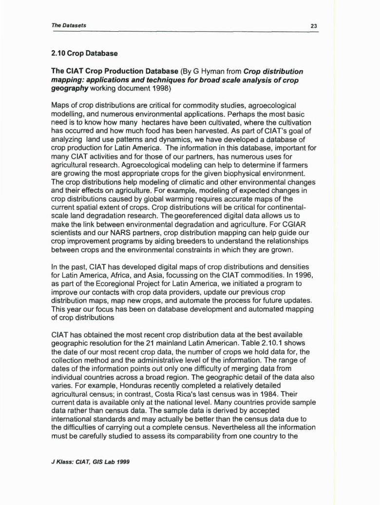
2.1 O Crop Data base

The CIAT Crop Production Database (By G Hyman from Crop distribution mapping: applications and techniques for broad sea/e analysis of crop geographyworking document 1998)

23

Maps of crop distributions are critica! for commodity studies, agroecological modelling, and numerous environmental applications. Perhaps the most basic need is to know how many hectares have been cultivated, where the cultivation has occurred and how much food has been harvested. As part of CIA T's goal of analyzing land use pattems and dynamics, we have developed a database of crop production for Latín America. The information in this database, important for many CIAT activities and for those of our partners, has numerous uses for agricultura! research. Agroecological modeling can help to determine if farmers are growing the most appropriate crops for the given biophysical environment. The crop distributions help modeling of climatic and other environmental changas and their effects on agricultura. For example, modeling of expected changas in crop distributions causad by global warming requires accurate maps of the current spatial extent of crops. Crop distributions will be critica! for continentalscale land degradation research. The georeferenced digital data allows us to make the link between environmental degradation and agricultura. For CGIAR scientists and our NARS partners, crop distribution mapping can help guide our crop improvement programs by aiding breeders to understand the relationships between crops and the environmental constraints in which they are grown.

In the past, CIAT has developed digital maps of crop distributions and densities for Latín America, Africa, and Asia, focussing on the CIAT commodities. In 1996, as part of the Ecoregional Project for Latín America, we initiated a program to improve our contacts with crop data providers, update our previous crop distribution maps, map new crops, and automate the process for future updates. This year our focus has been on data base development and automated mapping of crop distributions

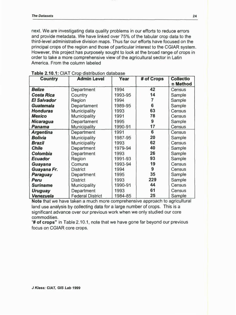
CIAT has obtained the most recent crop distribution data at the best available geographic resolution for the 21 mainland Latin American. Table 2.1 0.1 shows the date of our most recent crop data, the number of crops we hold data for, the collection method and the administrativa level of the information. The range of dates of the information points out only one difficulty of merging data from individual countries across a broad region. The geographic detail of the data also varíes. For example, Honduras recently completad a relatively detailed agricultura\ census; in contrast, Costa Rica's last census was in 1984. Their current data is available only at the national level. Many countries provide sample data rather than census data. The sample data is derivad by accepted intemational standards and m ay actually be better than the census data due to the difficulties of carrying out a complete census. Nevertheless all the information must be carefully studied to assess its comparability from one country to the


The Datasets 24

next. We are investigating data quality problems in our efforts to reduce errors and provide metadata. We ha ve linked over 75% of the tabular crop data to the third-level administrativa division maps. Thus far our efforts have focused on the principal crops of the region and those of particular interest to the CGIAR system. However, this project has purposely sought to look at the broad range of crops in order to take a more comprehensive view of the agricultura! sector in Latín America. From the column labeled

Tabla 2.10.1. CIAT Crop distribution database Country Admin Level Year

Belize Costa Rica El Salvador Guatemala Honduras Mexico Nicaragua Panama Argentina Bolivia Brazil Chile Colombia Ecuador Guaya na GuayanaFr. Paraguay Peru Suriname Uruguay Venezuela

Department Country Region Departament Municipality Municipality Departament Municipalitv Department Municipality Municipality Department Department Region Comuna District Department District Municipality Department Federal District

1994 1993-95 1994 1989-95 1993 1991 1995 1990-91 1991 1987-95 1993 1979-94 1993 1991-93 1993-94 1994 1995 1993 1990-91 1993 1984-85

# of Crops Collectio

42 14 7 6 63 78 9 17 6 20 62 40 26 93 19 9 35

229 44 61 25

n Method Census Sample Sample Sample Census Census Sample Census Census Sample Census Sample Sample Sample Census Census Sample Sample Census Census Sample

Note that we have taken a much more comprehens1ve approach to agncultural land use analysis by collecting data for a large number of crops. This is a significant advance over our previous work when we only studied our core commodities. "# of crops" in Table 2. 1 O .1, note that we ha ve gone far beyond our previous focus on CGIAR core crops.


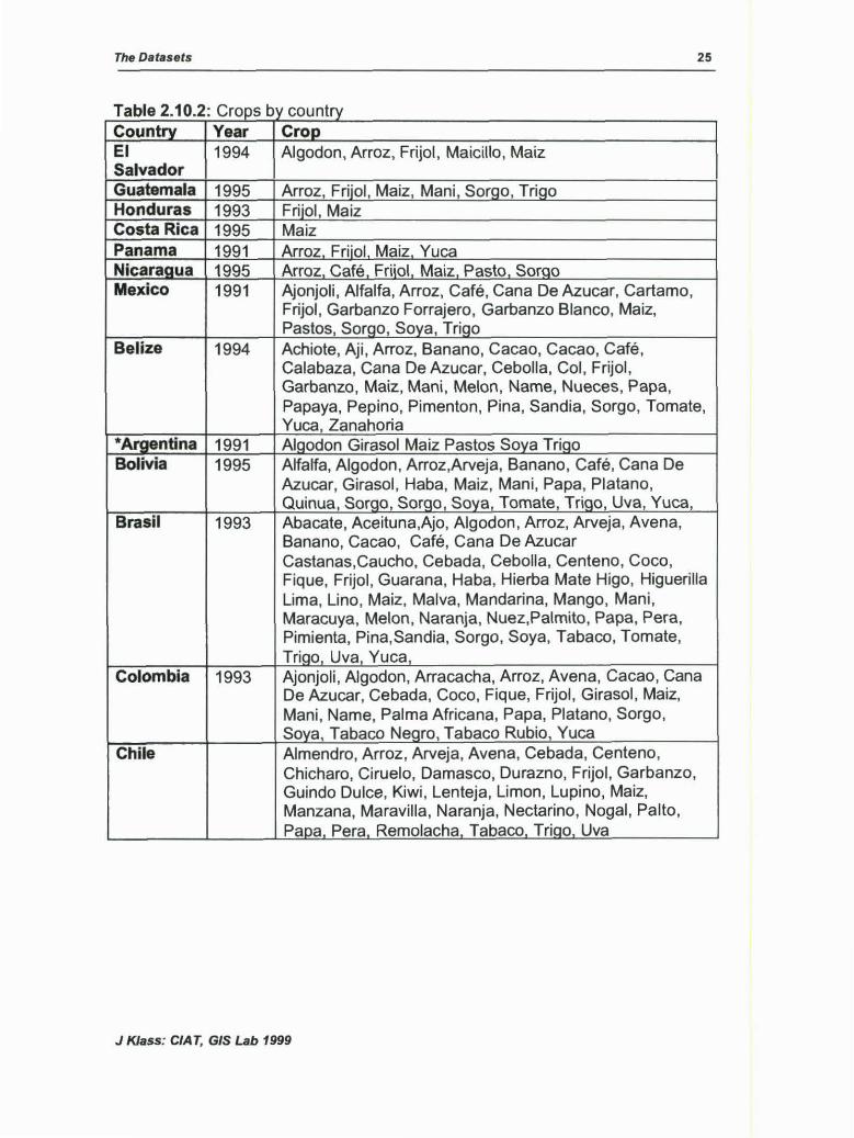
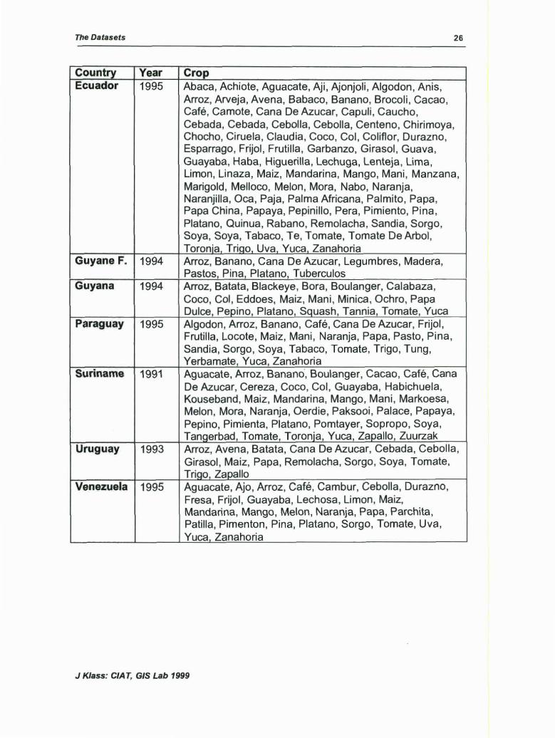
The Datasets 25

r bl 210 2 e b t a e . rops y country . . . Countrv Year Crop El 1994 Algodon, Arroz, Frijol, Maicillo, Maíz Salvador Guatemala 1995 Arroz Frijol, Maíz, Maní, Sorgo, Trigo Honduras 1993 Frijol, Maíz Costa Rica 1995 Maíz Panama 1991 Arroz Friiol Maíz Yuca Nicaragua 1995 Arroz Café~ Friiol Maíz Pasto Soroo Mexico 1991 Ajonjolí, Alfalfa, Arroz, Café, Cana De Azucar, Cartamo,

Frijol, Garbanzo Forrajero, Garbanzo Blanco, Maiz, Pastos, Sorgo, Soya, Trigo

Belize 1994 Achiote, Aji , Arroz, Banano, Cacao, Cacao, Café, Calabaza, Cana De Azucar, Cebolla, Col, Frijol , Garbanzo, Maíz, Maní, Melon, Name, Nueces, Papa, Papaya, Pepino, Pimenton, Pina, Sandía, Sorgo, Tomate, Yuca, Zanahoria

*Argentina 1991 Algodon Girasol Maiz Pastos Soya Trigo Bolivia 1995 Alfalfa, Algodon, Arroz,Arveja, Banano, Café, Cana De

Azucar, Girasol, Haba, Maiz, Mani, Papa, Platano, Quinua, Sorgo, Sorgo, Soya, Tomate, Trigo, Uva, Yuca,

Brasil 1993 Abacate, Aceituna,Ajo, Algodon, Arroz, Arveja, Avena, Banano, Cacao, Café, Cana De Azucar Castanas,Caucho, Cebada, Cebolla, Centeno, Coco, Fique, Frijol, Guarana, Haba, Hierba Mate Higo, Higuerilla Lima, Lino, Maiz, Malva, Mandarina, Mango, Mani, Maracuya, Melon, Naranja, Nuez,Palmito, Papa, Pera, Pimienta, Pina,Sandia, Sorgo, Soya, Tabaco, Tomate, Trioo Uva Yuca

Colombia 1993 Ajonjolí , Algodon, Arracacha, Arroz, Avena, Cacao, Cana De Azucar, Cebada, Coco, Fique, Frijol, Girasol, Maíz, Maní, Name, Palma Africana, Papa, Platano, Sorgo, Soya, Tabaco Negro, Tabaco Rubio, Yuca

Chile Almendro, Arroz, Arveja, Avena, Cebada, Centeno, Chícharo, Ciruelo, Damasco, Durazno, Frijol, Garbanzo, Guindo Dulce, Kiwi, Lenteja, Limon, Lupino, Maíz, Manzana, Maravilla, Naranja, Nectarino, Nogal, Palto, Papa Pera Remolacha Tabaco Trigo Uva


T11e Datasets 26

Country Year Crop Ecuador 1995 Abaca, Achiote, Aguacate, Aji , Ajonjoli, Algodon, Anis,

Arroz, Arveja, Avena, Babaco, Banano, Brocoli , Cacao, Café, Camote, Cana De Azucar, Capuli, Caucho, Cebada, Cebada, Cebolla, Cebolla, Centeno, Chirimoya, Chocho, Ciruela, Claudia, Coco, Col, Coliflor, Durazno, Esparrago, Frijol , Frutilla, Garbanzo, Girasol , Guava, Guayaba, Haba, Higuerilla, Lechuga, Lenteja, Lima, Liman, Linaza, Maiz, Mandarina, Mango, Mani, Manzana, Marigold, Melloco, Melon, Mora, Nabo, Naranja, Naranjilla, Oca, Paja, Palma Africana, Palmito, Papa, Papa China, Papaya, Pepinillo, Pera, Pimiento, Pina, Platano, Quinua, Rabano, Remolacha, Sandia, Sorgo, Soya, Soya, Tabaco, Te, Tomate, Tomate De Arbol, Toronja TriQo Uva Yuca Zanahoria

Guyane F. 1994 Arroz, Banano, Cana De Azucar, Legumbres, Madera, Pastos, Pina, Platano, Tuberculos

Guyana 1994 Arroz, Batata, Blackeye, Bora, Boulanger, Calabaza, Coco, Col, Eddoes, Maiz, Mani, Minica, Ochro, Papa Dulce, Pe_Qjno, Platano, Squash, Tannia, Tomate, Yuca

Paraguay 1995 Algodon, Arroz, Banano, Café, Cana De Azucar, Frijol , Frutilla, Locote, Maiz, Mani, Naranja, Papa, Pasto, Pina , Sandia, Sorgo, Soya, Tabaco, Tomate, Trigo, Tung, Yerbamate, Yuca, Zanahoria

Suriname 1991 Aguacate, Arroz, Banano', Boulanger, Cacao, Café, Cana De Azucar, Cereza, Coco, Col, Guayaba, Habichuela, Kouseband, Maiz, Mandarina, Mango, Mani, Markoesa, Melon, Mora, Naranja, Oerdie, Paksooi, Palace, Papaya, Pepino, Pimienta, Platano, Pomtayer, Sopropo, Soya, Tangerbad, Tomate, Toronja, Yuca, Zapallo, Zuurzak

Uruguay 1993 Arroz, Avena, Batata, Cana De Azucar, Cebada, Cebolla, Girasol, Maiz, Papa, Remolacha, Sorgo, Soya, Tomate, TriQo_, Zapallo

Venezuela 1995 Aguacate, Ajo, Arroz, Café, Cambur, Cebolla, Durazno, Fresa, Frijol , Guayaba, Lechosa, Liman, Maiz, Mandarina, Mango, Melon, Naranja, Papa, Parchita, Patilla, Pimenton, Pina, Platano, Sorgo, Tomate, Uva, Yuca Zanahoria

J Klass: C/A T, GIS La.b 1999

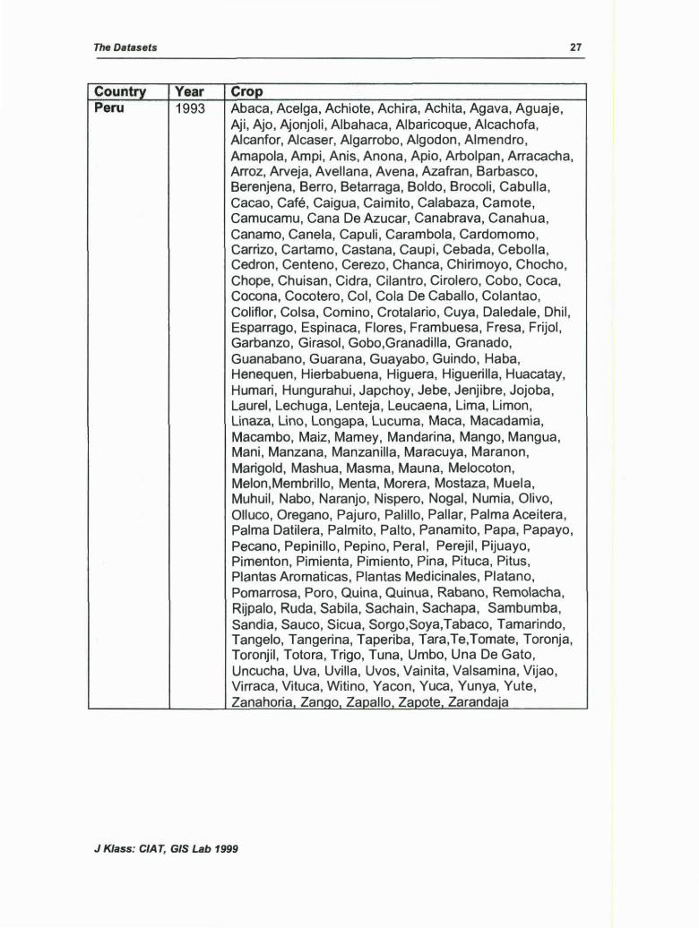
The Datasets 27

Country Year Crop Peru 1993 Abaca, Acelga, Achiote, Achira, Achita, Agava, Aguaje,

Aji, Ajo, Ajonjolí, Albahaca, Albaricoque, Alcachofa, Alcanfor, Alcaser, Algarrobo, Algodon, Almendro, Amapola, Ampi, Anis, Anona, Apio, Arbolpan, Arracacha, Arroz, Arveja, Avellana, Avena, Azafran, Barbasco, Berenjena, Berro, Betarraga, Boldo, Brocoli, Cabulla, Cacao, Café, Caigua, Caimito, Calabaza, Camote, Camucamu, Cana De Azucar, Cana brava, Canahua, Canamo, Canela, Capuli , Carambola, Cardomomo, Carrizo, Cartamo, Castana, Caupi, Cebada, Cebolla, Cedron, Centeno, Cerezo, Chanca, Chirimoyo, Chocho, Chope, Chuisan, Cidra, Cilantro, Cirolero, Coba, Coca, Cocona, Cocotero, Col, Cola De Caballo, Colantao, Coliflor, Colsa, Comino, Crotalario, Cuya, Daledale, Dhil, Esparrago, Espinaca, Flores, Frambuesa, Fresa, Frijol , Garbanzo, Girasol, Gobo,Granadilla, Granado, Guanabano, Guarana, Guayabo, Guindo, Haba, Henequen, Hierbabuena, Higuera, Higuerilla, Huacatay, Humari, Hungurahui, Japchoy, Jebe, Jenjibre, Jojoba, Laurel, Lechuga, Lenteja, Leucaena, Lima, Liman, Linaza, Lino, Longapa, Lucuma, Maca, Macadamia, Macambo, Maiz, Mamey, Mandarina, Mango, Mangua, Mani, Manzana, Manzanilla, Maracuya, Maranon, Marigold, Mashua, Masma, Mauna, Melocoton, Melon,Membrillo, Menta, Morera, Mostaza, Muela, Muhuil, Nabo, Naranjo, Níspero, Nogal, Numia, Olivo, Olluco, Oregano, Pajuro, Palillo, Paliar, Palma Aceitera, Palma Datilera, Palmito, Palto, Panamito, Papa, Papayo, Pecano, Pepinillo, Pepino, Peral, Perejil , Pijuayo, Pimenton, Pimienta, Pimiento, Pina, Pituca, Pitus, Plantas Aromaticas, Plantas Medicinales, Platano, Pomarrosa, Poro, Quina, Quinua, Rabano, Remolacha, Rijpalo, Ruda, Sabila, Sachain, Sachapa, Sambumba, Sandía, Sauco, Sicua, Sorgo,Soya,Tabaco, Tamarindo, Tangelo, Tangerina, Taperiba, Tara,Te,Tomate, Toronja, Toronjil, Totora, Trigo, Tuna, Umbo, Una De Gato, Uncucha, Uva, Uvilla, Uvas, Vainita, Valsamina, Vijao, Virraca, Vituca, Witino, Yacon, Yuca, Yunya, Yute, Zanahoria Zanga, Zapallo, Zapote Zarandaia


The Datasets

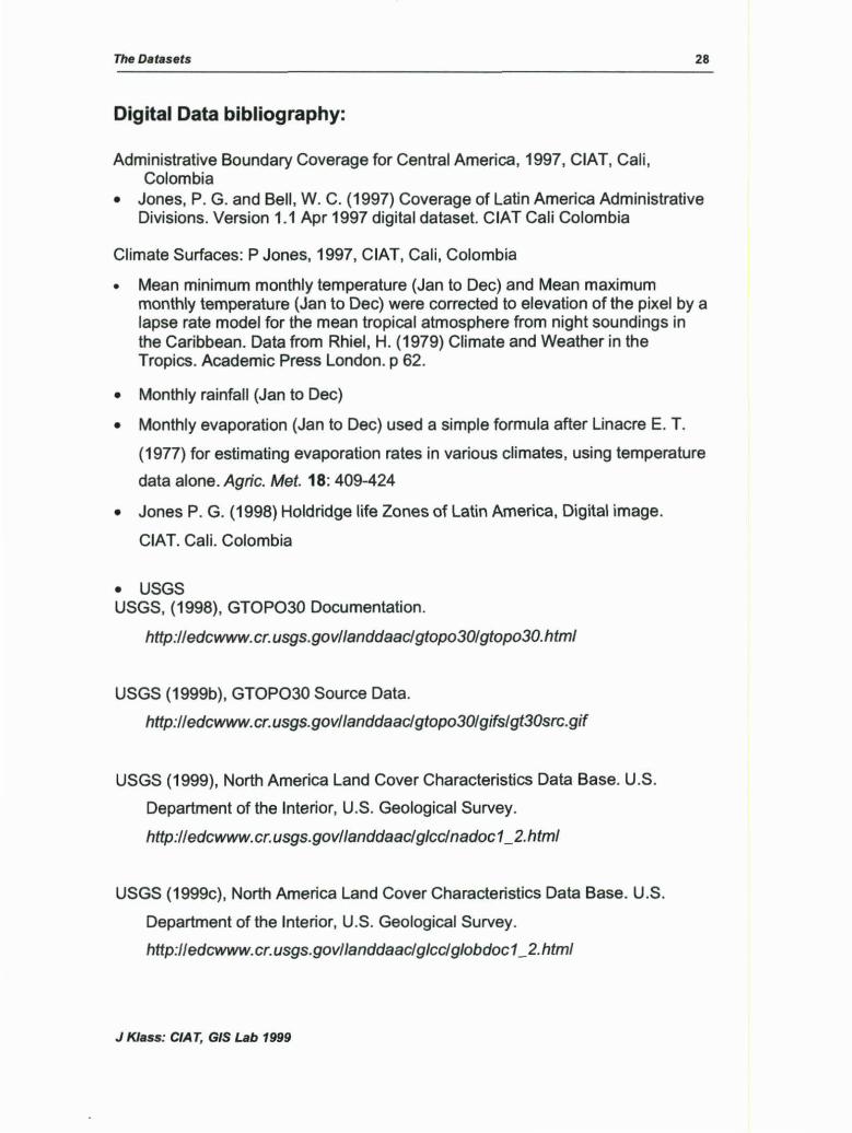
Digital Data bibliography:

Administrativa Boundary Coverage for Central America, 1997, CIAT, Cali, Colombia

28

• Jones, P. G. and Bell, W. C. (1997) Coverage of Latín America Administrativa Divisions. Version 1.1 Apr 1997 digital dataset. CIAT Cali Colombia

Climate Surfaces: P Jones, 1997, CIAT, Cali, Colombia

• Mean mínimum monthly temperatura (Jan to Dec) and Mean maximum monthly temperatura (Jan to Dec) were corrected to elevation of the pixel by a lapse rate model for the mean tropical atmosphere from night soundings in the Caribbean. Data from Rhiel, H. (1979) Climate and Weather in the Tropics. Academic Press London. p 62.

• Monthly rainfall (Jan to Dec)

• Monthly evaporation (Jan to Dec) used a simple formula after Linacre E. T.

(1977) for estimating evaporation rates in various climates, using temperatura

data alone. Agríe. Met. 18: 409-424

• Jones P. G. (1998) Holdridge lite Zones of Latín America, Digital image.

CIAT. Cali. Colombia

• USGS USGS, (1998), GTOP030 Documentation.

http://edcwww.cr.usgs.gov/landdaac/gtopo30/gtopo30.html

USGS (1999b), GTOP030 Source Data.

http://edcwww.cr.usgs.gov/landdaac/gtopo30/gifs/gt30src.gif

USGS (1999), North America Land Cover Characteristics Data Base. U.S.

Department of the Interior, U.S. Geological Survey.

http:l/edcwww.cr.usgs.gov/landdaac/glcc/nadoc1_2.htm/

USGS (1999c), North America Land Cover Characteristics Data Base. U.S.

Department of the Interior, U.S. Geological Survey.

http://edcwww.cr.usgs.gov/landdaac/glcc/g/obdoc1_2.html


The Datasets

USGS (1995}, Digital Chart of the World(DCW}, Defence Mapping Agency,

http:/1164.214.2.54/guides/dtf/dcw.htm/

Software

The data was collected by CIAT and the analysis was performed using the following software: ARC/INFO, ArcView GIS 3.1, ldrisi, PCI, Splus and Excel.


29

ciat data documentation

Documents