chapter 5 – the acoustic wave equation and simple...

Oelze ECE/TAM 373 Notes - Chapter 5 pg 1

Chapter 5 – The Acoustic Wave Equation and Simple Solutions

(5.1) In this chapter we are going to develop a simple linear wave equation for sound propagation in fluids (1D). In reality the acoustic wave equation is nonlinear and therefore more complicated than what we will look at in this chapter. However, in most common applications, the linear approximation to the wave equation is a good model. Only when sound waves have high enough amplitude do nonlinear effects show themselves. What is an acoustic wave? It is essentially a pressure change. A local pressure change causes immediate fluid to compress which in turn causes additional pressure changes. This leads to the propagation of an acoustic wave. Before we derive the wave equation, let’s cover a few definitions and concepts. Generation ® Transducer (piston for example) creates a particle displacement (which in turn has an associated pressure and density change). This change affects the immediately adjacent region, etc., so that the disturbance (wave) propagates. Uniform plane wave ® common phase and amplitude in a plane ^ direction of propagation. Particle We will talk a lot about particle displacement. It is defined in terms of continuum

mechanics. A particle contains many molecules (large enough to be considered as a continuous medium) but its dimensions are small compared to the distances for significant changes in the acoustic parameters (for example, small compared to l or small enough to consider acoustic variables constant throughout particle volume).

Parameters acoustic pressure particle displacement particle velocity particle acceleration density changes velocity potential particle position particle displacement

particle velocity

density r

ˆ ˆ ˆr x x y y z z= + +!

ˆ ˆ ˆx y zx y zx x x x= + +!

tu x

¶=¶!!


condensation

undisturbed (equilibrium) density acoustic pressure instantaneous undisturbed (ambient pressure) pressures Three laws used to develop wave equation for fluids

1) Equation of State – determined by thermodynamic properties Relates changes in Pressure (P) and density (r). Dependent upon material (for example, an ideal gas is different from a liquid). We can expand the Equation of state into linear and nonlinear terms, however, we will only

be looking at the linear terms (for now). 2) Equation of Continuity – Essentially this is conservation of mass. Relative Motion of fluid in

a volume causes change in density. 3) Equation of Motion – Force Equation – Newton’s 2nd law Pressure variations generate a force (F = P ´ Area) that causes particle motion

(5.2) Let’s first look at the Equation of State: An equation of state must relate three physical quantities describing the thermodynamic behavior of the fluid. For example, the equation of state for a perfect gas is

where P is the pressure in Pascals, r is the density (kg/m3), r is the gas constant, and TK is the temperature in Kelvin. If the gas has high thermal conductivity then any slow compressions of the gas will be isothermic and

.

If the thermal conductivity is sufficiently low, the heat conduction during a cycle of the acoustic disturbance becomes negligible. In this case the condition is considered adiabatic and the relation between the pressure and density for the perfect gas are:

where g is the ratio of specific heats, .

0

0

–s r rr

=

0–p P P=

KP rTr=

0 0

PP

rr

=

0 0

PP

grr

æ ö= ç ÷è ø

p

v

CC


The perfect gas is a simple case for an adiabat. To model this relationship, let expand P as a function of r (about r0) in a Taylor series:

The Taylor series shows the fluctuations of P with r. We can rewrite this as:

where

,

.

The Taylor series is nonlinear due to the quadratic term (r-r0)2 . The nonlinearity of a propagation medium is usually characterized by the ratio of B/A. We linearize the Taylor series by assuming small fluctuations so that only the lowest order term in

need be retained. This gives: where we define the coefficient A as the adiabatic bulk modulus, B:

Let’s examine the unit for

P : Pascal where 1Pa = 1 N/m2 = 1kg /s2/m

r : kg/m3

®

® (speed) (experimentally determined)

so

is the Equation of State for linear acoustic waves in fluids (small changes in density |s| << 1).

( ) ( )0 0

22

0 0 02

1 ...2

P P PPr r

r r r rr r

æ öæ ö¶ ¶+ - + - +ç ÷ç ÷¶ ¶è ø è ø

=

2 30

1 1 ...2 3!

P P As Bs Cs= + + + +

0

0PA

r

rr

æ ö¶= ç ÷¶è ø

0

220 2

PBr

rr

æ ö¶= ç ÷¶è ø

( )0r r-

0p P P As= - =

0

0PA

r

rr

æ ö¶= = ç ÷¶è øB

0

0P

r

rr

æ ö¶= ç ÷¶è ø

B

Pr

2

2

ms

Pr

2c

20p c s sr= = B


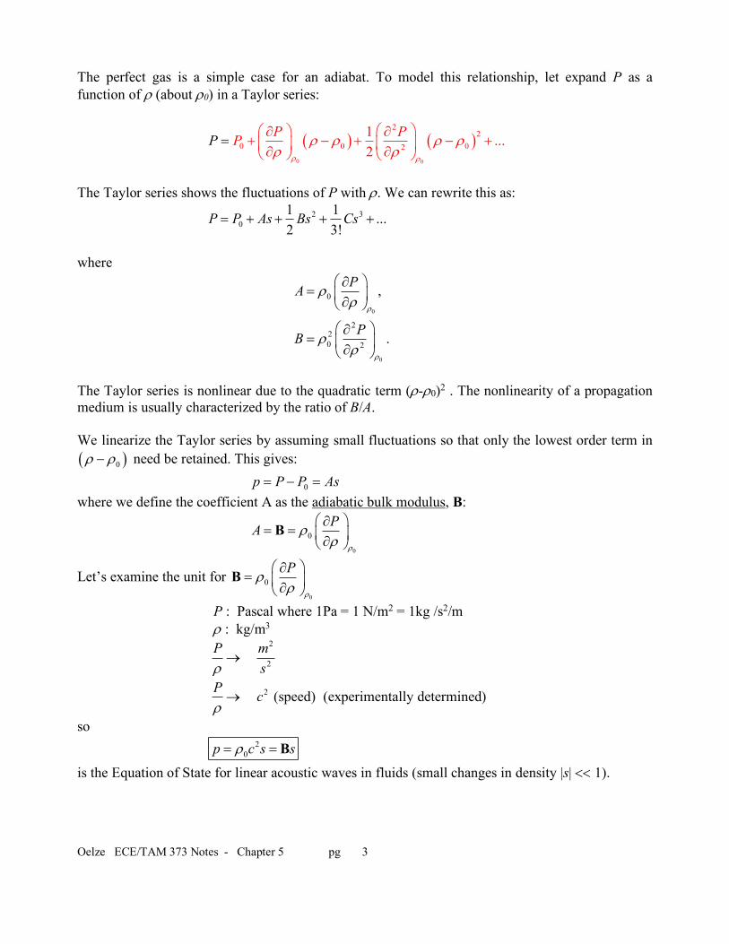
*************************** Example 5.1 *************************** Compare the condensation for water and air at 20˚C if the pressure change is 1 atm: Sol: p = Bs = r0c

2s From tables: for fresh water @ 20˚C: r0 = 998 kg/m3 and c = 1481 m/s For p = 1 atm = 1.0133 bar = 1.0133 ´ 105 Pa

for air @ 20˚C: r0 = 1.21 kg/m3 and c = 343 m/s

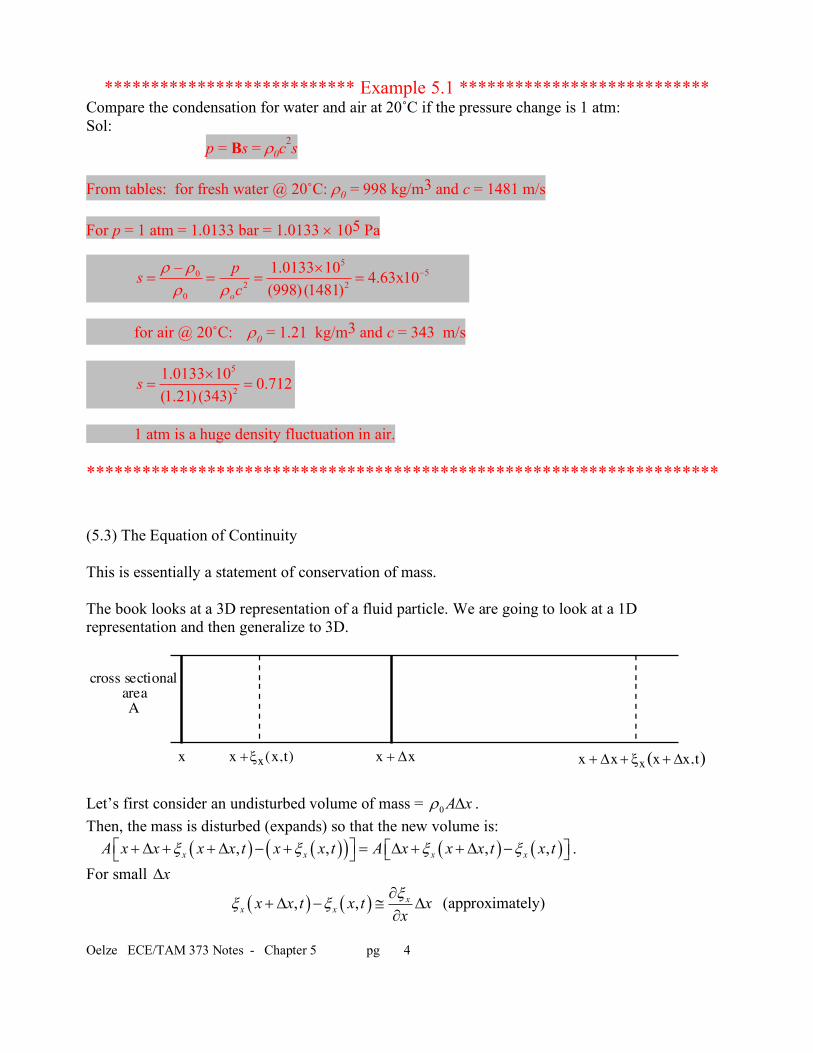
1 atm is a huge density fluctuation in air. ******************************************************************** (5.3) The Equation of Continuity This is essentially a statement of conservation of mass. The book looks at a 3D representation of a fluid particle. We are going to look at a 1D representation and then generalize to 3D.

Let’s first consider an undisturbed volume of mass = . Then, the mass is disturbed (expands) so that the new volume is: . For small

(approximately)

550

2 20

– 1.0133 10 4.63x10(998) (1481)o

psc

r rr r

-´= = = =

5

2

1.0133 10 0.712(1.21) (343)

s ´= =

cross sectionalareaA

x x +xx(x,t) x + Dx x + Dx+ xx x+ Dx,t( )

0A xr D

( ) ( )( ) ( ) ( ), , , ,x x x xA x x x x t x x t A x x x t x tx x x xé ù+D + +D - + = D + +D -é ùë ûë ûxD

( ) ( ), , xx xx x t x t x

xxx x ¶

+ D - @ D¶


giving the new volume

.

Our disturbed density will then be

.

Now, recall that the condensation is:

.

Solving for the total density gives . Substituting into our equation above yields

or rearranging

.

If we assume that and are small so that the second term is negligible (most often the case).

Notice that the condensation, , is the fractional change in density. This equation tells us that if the displacement, , varies with x then there is a density change. The minus sign is significant. If the displacement increases with x what happens to the density? Why? If we generalize the equation to 3-D we get

or

If we differentiate with respect to time

we note that and so

1 xA xxx¶æ öD +ç ÷¶è ø

massvolume

r =

00

11 x

x

A x

A x xx

rrx

xr rD=

¶æ öD +

¶æ ö® = +ç ÷¶÷ø

è¶è

øç

0

0

–s r rr

=

0 0sr r r= +

( )0 0 0 1 xsxxr r r ¶æ ö= + +ç ÷¶è ø

0 0 0x xs sx xx xr r r¶ ¶

= - -¶ ¶

s x

xx¶¶

xsxx¶

= -¶

sxx

yx zsx y z

xx x¶¶ ¶= - - -

¶ ¶ ¶

( )ˆ ˆ ˆ ˆˆ ˆx y zs x y z x y zx y z

x x xæ ö¶ ¶ ¶

= - + + × + +ç ÷¶ ¶ ¶è øs x= -Ñ×

!

( )st

x¶= -Ñ×

¶

!

( )t txx¶ ¶

-Ñ× = -Ñ×¶ ¶

!!

utx¶=

¶

!!


. (the linear equation of continuity)

or alternatively if we substitute in for the density we have:

.

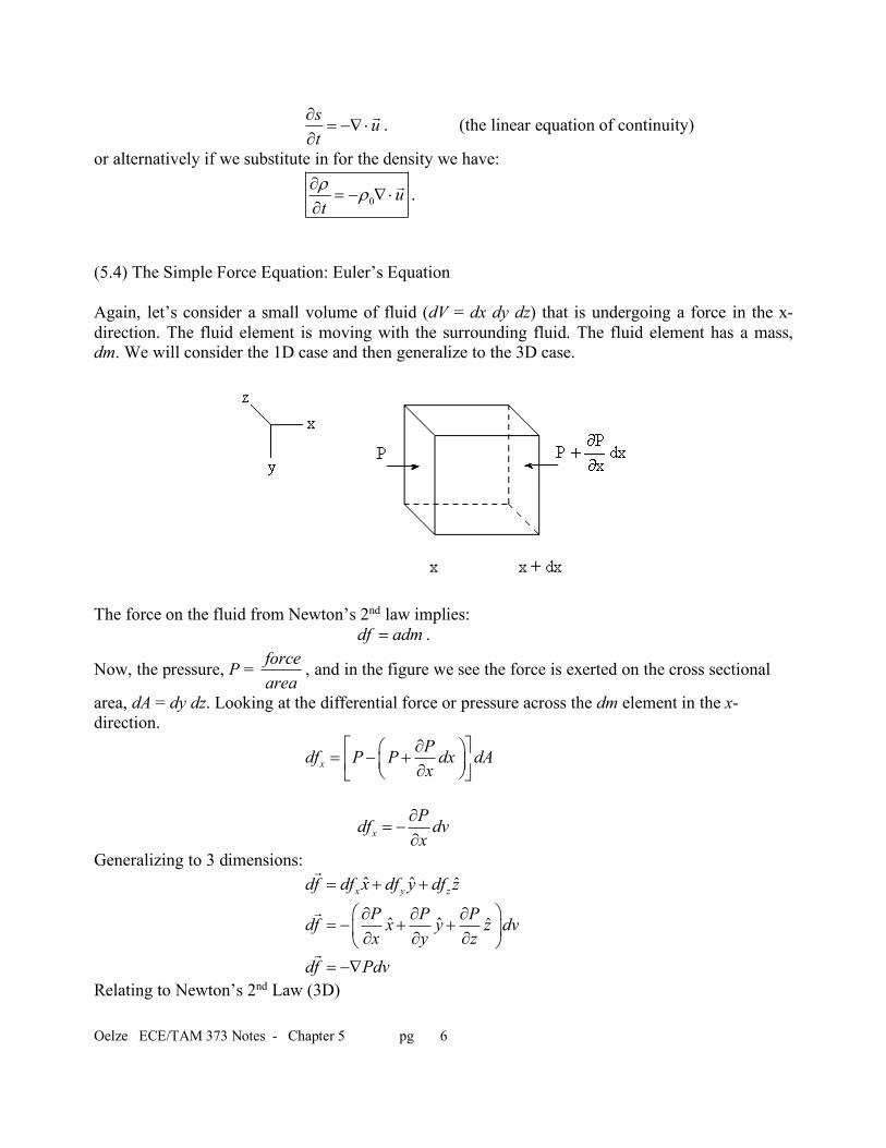
(5.4) The Simple Force Equation: Euler’s Equation Again, let’s consider a small volume of fluid (dV = dx dy dz) that is undergoing a force in the x-direction. The fluid element is moving with the surrounding fluid. The fluid element has a mass, dm. We will consider the 1D case and then generalize to the 3D case.

The force on the fluid from Newton’s 2nd law implies: .

Now, the pressure, P = , and in the figure we see the force is exerted on the cross sectional

area, dA = dy dz. Looking at the differential force or pressure across the dm element in the x-direction.

Generalizing to 3 dimensions:

Relating to Newton’s 2nd Law (3D)

s ut¶

= -Ñ×¶

!

0 utr r¶= - Ñ×

¶!

df adm=forcearea

xPdf P P dx dAx

é ¶ ùæ ö= - +ç ÷ê ú¶è øë û

xPdf dvx¶

= -¶

ˆ ˆ ˆx y zdf df x df y df z= + +!

ˆ ˆ ˆP P Pdf x y z dvx y z

æ ö¶ ¶ ¶= - + +ç ÷¶ ¶ ¶è ø

!

df Pdv= -Ñ!


where

.

Recall, there is a difference between

and .

or simplifying

.

Using the fact that then relating the forces gives

This is the nonlinear, inviscid force equation (viscosity introduced later as a loss mechanism). To get the linear Euler’s equation we will retain only the 1st order terms. 1st: .

2nd: The particle velocity is assumed small so terms of 2nd order are negligible giving:

3rd: If we assume that |s| << 1 (small) then giving finally:

(linear Euler’s equation, Newtons’s Law)

(5.5) The Linearized Wave Equation (1) Equation of State (Linearized):

Where

df adm=! !

duadt

=!

!

dudt

! ut

¶¶

!

du u x u y u z udt x t y t z t t

¶ ¶ ¶ ¶ ¶ ¶ ¶= + + +¶ ¶ ¶ ¶ ¶ ¶ ¶

! ! ! ! !

x y zdu u u u uu u udt x y z t

¶ ¶ ¶ ¶= + + +¶ ¶ ¶ ¶

! ! ! ! !

( )du ua u udt t

¶= = ×Ñ +

¶

! !! ! !

dm dvr=

( ) uPdv u u dvt

r ¶é ù-Ñ = ×Ñ +ê ú¶ë û

!! !

( ) uP u ut

r ¶é ù-Ñ = ×Ñ +ê ú¶ë û

!! !

0p P P p P= - ® Ñ =Ñ

upt

r ¶-Ñ =¶

!

0r r=

0upt

r ¶-Ñ =

¶

!

20p s c sr= =B

0

0P

r

rr

æ ö¶= ç ÷¶è ø

B


(2) Continuity Equation (Linearized):

(3) Euler’s Equation (Linearized):

To derive the Linear Wave Equation we first take the derivative of s

Recall

So that or .

Substituting this into the Continuity Equation (2) gives the relative change in density as the divergence of the particle velocity.

Substituting in the Equation of State (1) yields

(4)

Taking the derivative of (4) wrt time gives:

. (5)

If we take the divergence of Euler’s Equation (3):

.

Substituting into (5) gives the result:

Using gives us the Linearized Wave Equation:

This is also (in form) the Classical Wave Equation! The speed of sound is given by: c2 We can also define a velocity potential (similar to EM).

0 utr r¶= - Ñ×

¶!

0upt

r ¶-Ñ =

¶

!

0

0

s r rr-

=

0

1ds ddt dt

rr

= 0d dsdt dtr r=

0 0s ut

r r¶= - Ñ×

¶!

p ut¶ é ù = -Ñ×ê ú¶ ë ûB

!

p ut¶

= - Ñ×¶

B !

2

2

p uut t t

¶ ¶ ¶= - Ñ× = - Ñ×

¶ ¶ ¶B B

!!

0upt

r ¶é ùÑ × -Ñ =ê ú¶ë û

!

2

0

1 uptr

¶- Ñ =Ñ×

¶

!

22

20

p pt r

¶= Ñ

¶B

20cr=B

22 2

2

p c pt

¶= Ñ

¶


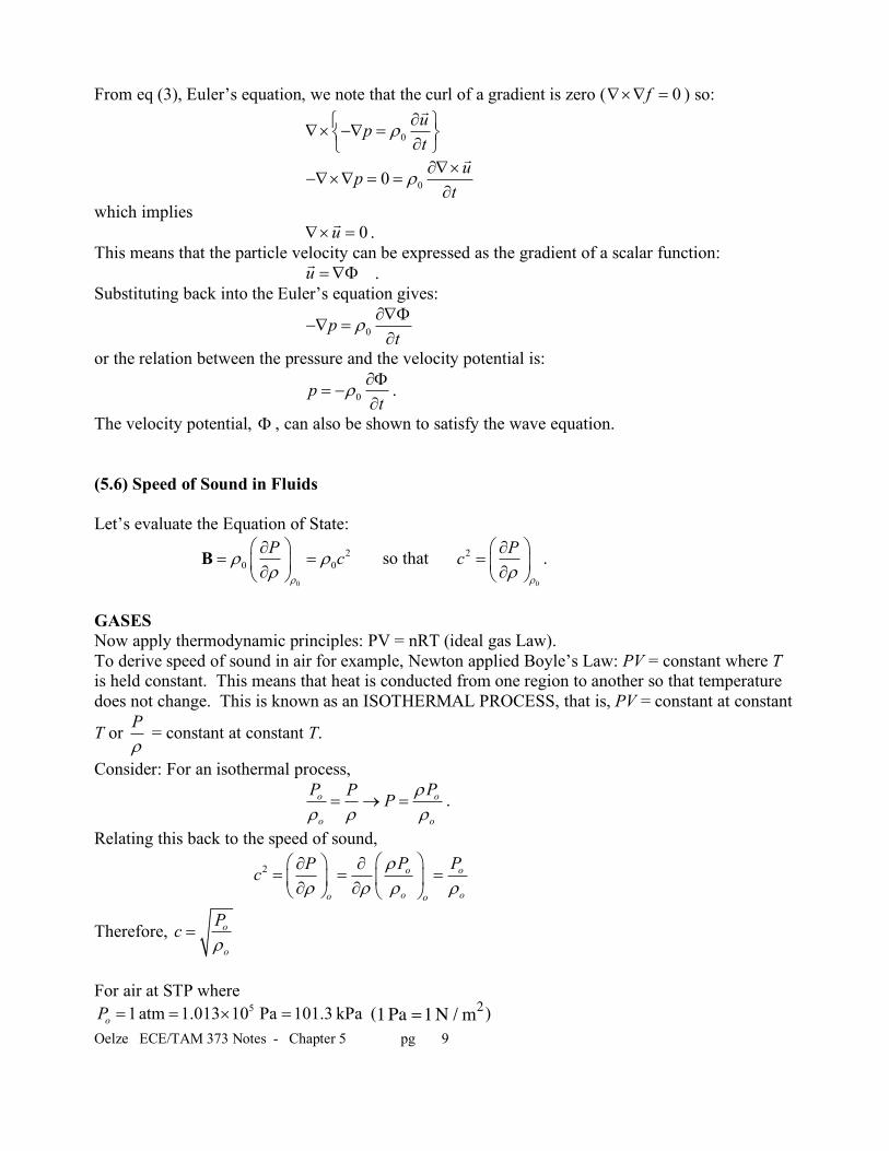
From eq (3), Euler’s equation, we note that the curl of a gradient is zero ( ) so:

which implies . This means that the particle velocity can be expressed as the gradient of a scalar function: . Substituting back into the Euler’s equation gives:

or the relation between the pressure and the velocity potential is:

.

The velocity potential, , can also be shown to satisfy the wave equation. (5.6) Speed of Sound in Fluids Let’s evaluate the Equation of State:

so that .

GASES Now apply thermodynamic principles: PV = nRT (ideal gas Law). To derive speed of sound in air for example, Newton applied Boyle’s Law: PV = constant where T is held constant. This means that heat is conducted from one region to another so that temperature does not change. This is known as an ISOTHERMAL PROCESS, that is, PV = constant at constant

T or = constant at constant T.

Consider: For an isothermal process,

.

Relating this back to the speed of sound,

Therefore,

For air at STP where

( )

0fÑ´Ñ =

0upt

r ¶ì üÑ´ -Ñ =í ý¶î þ

!

00 upt

r ¶Ñ´-Ñ´Ñ = =

¶

!

0uÑ´ =!

u =ÑF!

0pt

r ¶ÑF-Ñ =

¶

0pt

r ¶F= -

¶F

0

20 0

P cr

r rr

æ ö¶= =ç ÷¶è ø

B0

2 Pcrr

æ ö¶= ç ÷¶è ø

Pr

o o

o o

P PP P rr r r

= ® =

2 o o

o oo o

P PPc rr r r r

æ öæ ö¶ ¶= = =ç ÷ç ÷¶ ¶è ø è ø

o

o

Pcr

=

51atm 1.013 10 Pa 101.3 kPaoP = = ´ = 1Pa =1N / m2


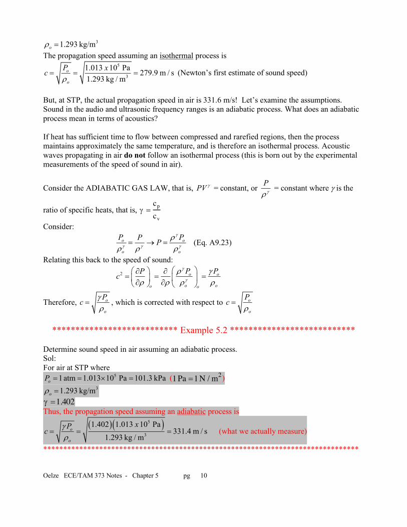
The propagation speed assuming an isothermal process is

(Newton’s first estimate of sound speed)

But, at STP, the actual propagation speed in air is 331.6 m/s! Let’s examine the assumptions. Sound in the audio and ultrasonic frequency ranges is an adiabatic process. What does an adiabatic process mean in terms of acoustics? If heat has sufficient time to flow between compressed and rarefied regions, then the process maintains approximately the same temperature, and is therefore an isothermal process. Acoustic waves propagating in air do not follow an isothermal process (this is born out by the experimental measurements of the speed of sound in air).

Consider the ADIABATIC GAS LAW, that is, = constant, or = constant where g is the

ratio of specific heats, that is,

Consider:

(Eq. A9.23)

Relating this back to the speed of sound:

Therefore, , which is corrected with respect to

*************************** Example 5.2 ***************************

Determine sound speed in air assuming an adiabatic process. Sol: For air at STP where

( )

Thus, the propagation speed assuming an adiabatic process is

(what we actually measure)

*******************************************************************************

31.293 kg/mor =

5

3

1.013 10 Pa 279.9 m / s1.293 kg / m

o

o

P xcr

= = =

PV g Pgr

g =cpcv

o o

o o

P PP Pg

g g g

rr r r

= ® =

2 o o

o oo o

P PPcg

g

r gr r r r

æ öæ ö¶ ¶= = =ç ÷ç ÷¶ ¶è ø è ø

o

o

Pc gr

= o

o

Pcr

=

51atm 1.013 10 Pa 101.3 kPaoP = = ´ = 1Pa =1N / m231.293 kg/mor =

g =1.402

( )( )5

3

1.402 1.013 10 Pa331.4 m / s

1.293 kg / mo

o

xPc gr

= = =


Combining the Equation of State (perfect gas law or ideal gas equation - see Eq 5.2.1 or Eq A9.17)

and the expression for propagation speed (adiabatic assumption) yields

where r is the gas constant for a particular gas

Eq A9.17

the universal gas constant = 8314 J/(kg-˚K) = 8.315 J/(mol-˚K) M = average molecular weight (weighting corresponding to the fraction by volume of the total number of molecules) k the Boltzmann’s constant = 1.381 x 10-23 J/˚K

is the mass of 1 atomic mass unit = 1.661 x 10-27 kg is the average mass per molecule

For Air: Mixture for dry air by volume is 78% N2 - Molecular weight = 28 21% O2 - Molecular weight = 32 1% Argon - Molecular weight = 40 M = (0.78)(28) + (0.21)(32) + (0.01)(40) = 28.96

d = # of excited degrees of freedom and d = 5 for both N2 and O2 (3 translational and 2 rotational)

= 331.4 m/s

Note unit:

kP rTr= o

o

Pc gr

=

( )o kok

o o

rTPc rTg rg g

r r= = =

amuo

av

amu

kmRr

M mm

æ öç ÷è ø= =æ öç ÷è ø

oR

amum

avm

oo8314 J /(kg - K) 287.1 J /(kg - K)

28.96oRrM

= ==

2 5 2 7 1.45 5

dd

g + += = = =

( )( )( )1.4 287.1 /( ) 273.16ko oJ kg K Kc= γrT -=

Jkg

=N ×mkg

=kg×m / s2( )×m

kg=

m2

s2=ms


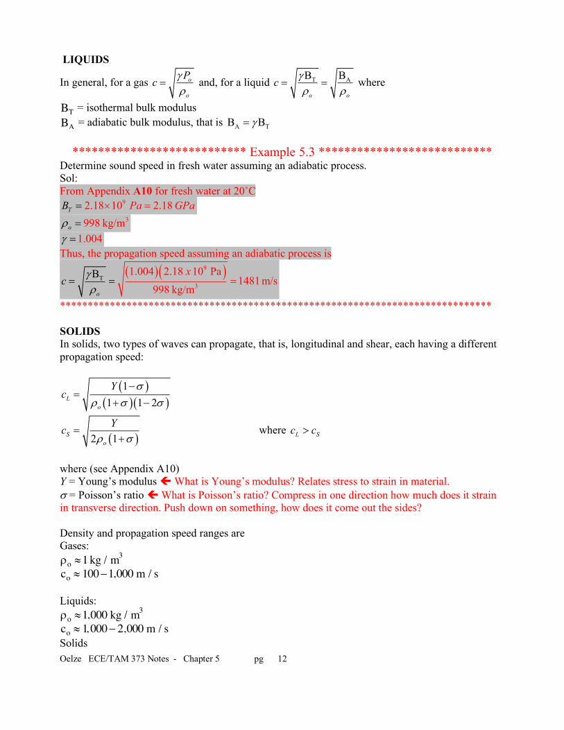
LIQUIDS

In general, for a gas and, for a liquid where

= isothermal bulk modulus = adiabatic bulk modulus, that is

*************************** Example 5.3 ***************************

Determine sound speed in fresh water assuming an adiabatic process. Sol: From Appendix A10 for fresh water at 20˚C

Thus, the propagation speed assuming an adiabatic process is

****************************************************************************** SOLIDS In solids, two types of waves can propagate, that is, longitudinal and shear, each having a different propagation speed:

where

where (see Appendix A10) Y = Young’s modulus ç What is Young’s modulus? Relates stress to strain in material. s = Poisson’s ratio ç What is Poisson’s ratio? Compress in one direction how much does it strain in transverse direction. Push down on something, how does it come out the sides? Density and propagation speed ranges are Gases:

Liquids:

Solids

o

o

Pc gr

= T AB B

o o

c gr r

= =

BTBA A TB Bg=

92.18 10 2.18T Pa PB G a´ ==3998 kg/mor =

1.004g =

( )( )T9

3

1.004 2.18 10 Pa1481m/s

998 kB

g/mo

cxg

r= ==

( )( )( )

11 1 2L

o

Yc

sr s s

-=

+ -

( )2 1So

Ycr s

=+ L Sc c>

ro »1kg / m3

co » 100-1,000 m / s

ro »1,000 kg / m3

co » 1, 000- 2,000 m / s


(Longitudinal or Bulk)

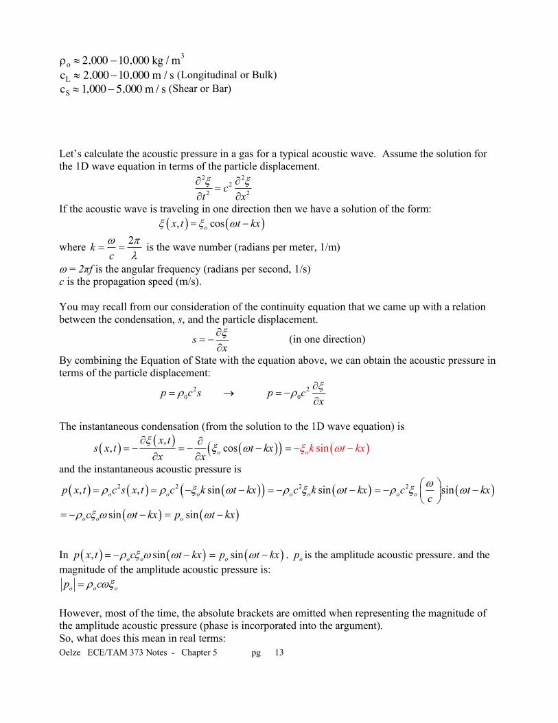
(Shear or Bar) Let’s calculate the acoustic pressure in a gas for a typical acoustic wave. Assume the solution for the 1D wave equation in terms of the particle displacement.

If the acoustic wave is traveling in one direction then we have a solution of the form:

where is the wave number (radians per meter, 1/m)

w = 2πf is the angular frequency (radians per second, 1/s) c is the propagation speed (m/s). You may recall from our consideration of the continuity equation that we came up with a relation between the condensation, s, and the particle displacement.

(in one direction)

By combining the Equation of State with the equation above, we can obtain the acoustic pressure in terms of the particle displacement:

®

The instantaneous condensation (from the solution to the 1D wave equation) is

and the instantaneous acoustic pressure is

In , is the amplitude acoustic pressure, and the magnitude of the amplitude acoustic pressure is:

However, most of the time, the absolute brackets are omitted when representing the magnitude of the amplitude acoustic pressure (phase is incorporated into the argument). So, what does this mean in real terms:

ro » 2,000 -10,000 kg / m3

cL » 2,000-10,000 m / scS » 1,000- 5,000 m / s

2 22

2 2ct xx x¶ ¶=

¶ ¶

( ) ( ), cosox t t kxx x w= -

2kcw p

l= =

sxx¶

= -¶

20p c sr= 2

0p cxxr ¶

= -¶

( ) ( ) ( )( ),, coso

x ts x t t kx

x xx

x w¶ ¶

= - = - -¶ ¶

( )sinok t kxx w -= -

( ) ( ) ( )( )2 2, , sino o op x t c s x t c k t kxr r x w= = - - ( )2 sino oc k t kxr x w= - - ( )2 sino oc t kxcwr x wæ ö= - -ç ÷è ø

( )sino oc t kxr x w w= - - ( )sinop t kxw= -

( ) ( ), sino op x t c t kxr x w w= - - ( )sinop t kxw= - op

o o op cr wx=


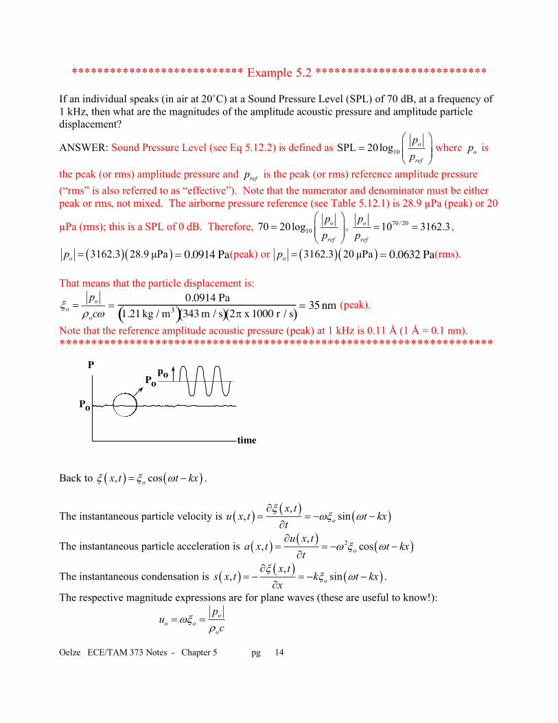
*************************** Example 5.2 ***************************

If an individual speaks (in air at 20˚C) at a Sound Pressure Level (SPL) of 70 dB, at a frequency of 1 kHz, then what are the magnitudes of the amplitude acoustic pressure and amplitude particle displacement?

ANSWER: Sound Pressure Level (see Eq 5.12.2) is defined as where is

the peak (or rms) amplitude pressure and is the peak (or rms) reference amplitude pressure (“rms” is also referred to as “effective”). Note that the numerator and denominator must be either peak or rms, not mixed. The airborne pressure reference (see Table 5.12.1) is 28.9 µPa (peak) or 20

µPa (rms); this is a SPL of 0 dB. Therefore, , ,

(peak) or (rms). That means that the particle displacement is:

(peak).

Note that the reference amplitude acoustic pressure (peak) at 1 kHz is 0.11 Å (1 Å = 0.1 nm). ********************************************************************

Back to .

The instantaneous particle velocity is

The instantaneous particle acceleration is

The instantaneous condensation is .

The respective magnitude expressions are for plane waves (these are useful to know!):

10SPL 20log o

ref

pp

æ ö= ç ÷ç ÷

è øop

refp

1070 20log o

ref

pp

æ ö= ç ÷ç ÷

è ø

70/ 2010 3162.3o

ref

pp

= =

( )( )3162.3 28.9 µPaop = = 0.0914 Pa ( )( )3162.3 20 µPaop = = 0.0632 Pa

oo

o

pc

xr w

= =0.0914 Pa

1.21 kg / m3( )343m / s( ) 2p x1000 r / s( )= 35nm

( ) ( ), cosox t t kxx x w= -

( ) ( ) ( ),, sino

x tu x t t kx

tx

wx w¶

= = - -¶

( ) ( ) ( )2,, coso

u x ta x t t kx

tw x w

¶= = - -

¶

( ) ( ) ( ),, sino

x ts x t k t kx

xx

x w¶

= - = - -¶

oo o

o

pu

cwx

r= =

time

P

Po

poPo


*************************** Example 5.2 ***************************

If an individual speaks (in air at 20˚C) at a Sound Pressure Level (SPL) of 70 dB, at a frequency of 1 kHz, then what are the magnitudes of the amplitude particle velocity, amplitude particle acceleration and amplitude condensation? ANSWER: Using information from the previous example, magnitudes (peak values) of the amplitude particle velocity is 2.20x10-4 m/s, amplitude particle acceleration is 1.38 m/s2 and amplitude condensation is 6.72x10-7. Small… ******************************************************************** A significant parameter in nonlinear acoustics and what is called shock wave theory is the Mach number (see Problem 5.7.1 in Kinsler et al). Based on the parameters introduced already, the Mach

number is defined as . Note how this compares to the magnitude of condensation:

2 oo o o

o

pa u

cw

w w xr

= = =

2oo o

o oo

pus kc c c

wxxr

= = = =

ouMc

=

2oo o

o oo

pus kc c c

wxxr

= = = =

chapter 5 – the acoustic wave equation and simple...

Documents