mathematical musical physics of the wave … musical physics of the wave ... etc. to the 3-d wave...
TRANSCRIPT
UIUC Physics 406 Acoustical Physics of Music
Professor Steven Errede, Department of Physics, University of Illinois at Urbana-
Champaign, Illinois 2002-2017. All rights reserved.
1
Mathematical Musical Physics of the Wave Equation – Part 2
C. Standing Waves In Three-Dimensional Systems:
Before “diving in” on discussing specific, but still simple systems exhibiting acoustical standing wave phenomena in three dimensions, we make a few brief comments that are relevant/ common to all such systems. First, there are (at least) two general perspectives associated with acoustical standing waves in 3-dimensional systems. For (idealized) three dimensional membrane-like structures (e.g. idealized 3-D “drums”), one is interested in solving the appropriate two-dimensional wave equation, with appropriate boundary conditions, in order to obtain the standing wave eigen-solutions, etc. associated with transverse displacement of the 2-D membrane surfaces on a 3-D structure as a function of any/all positions on these surfac(es) and as a function of time. We will not discuss these here. We will discuss finding the eigen-solutions, etc. to the 3-D wave equation associated with longitudinal acoustic standing waves confined within the interior region of a (rigid) 3-D structure (e.g. idealized 3-D “organ pipes”), which of course are associated with longitudinal displacement and/or (over-)pressure standing waves in the air inside the interior of the 3-D structure. In addition, these situations are also eminently applicable to fluid-filled and/or elastic solid 3-D structures.
Note that longitudinal acoustic standing waves in 3-D “organ pipe”-like structures are excited by air flow, and hence pressure should rightly be viewed as the primary physical parameter, solving the (over-)pressure wave equation with appropriate boundary conditions ( / 0p n , where n is the normal (i.e. perpendicular) direction to the local {matter} surface {if present}) and then relating the eigen-solutions associated with longitudinal pressure standing waves to those associated with the longitudinal displacement amplitude, via use of the (appropriately modified) ( , ) ( , )airp r t B r t
.
However, one can instead solve the wave equation with the appropriate boundary conditions for longitudinal displacement amplitude at the internal boundaries of the 3-D structure to obtain the eigen-solutions, etc. describing longitudinal displacement amplitude standing waves confined within the interior of the structure, and then use the above (over-) pressure – gradient-of-longitudinal displacement relation to obtain the eigen-solutions associated with the (over-) pressure longitudinal standing waves.
There is actually a deep physical principle operative here, to explain why this works. At the microscopic (i.e. atomic) level, the collision(s) of air molecules with each other, arising from the presence of additional energy (provided by the presence of the acoustic standing waves internal to the 3-D structure), all involve elastic scattering of air molecules with each other, and with the atoms making up the interior walls of the 3-D structure. All such elastic scatterings of atoms with other atoms manifestly involves the electromagnetic force – one of the four (known) fundamental forces of nature. At the microscopic/atomic/elementary particle level, the electromagnetic force manifestly obeys time-reversal invariance – i.e. microscopically, the physics is exactly the same whether time goes forward or backward. A person watching a movie of atoms/molecules elastically scattering off of one another (via the electromagnetic interaction) in this physical situation cannot tell/determine whether time is going forward or backward.

UIUC Physics 406 Acoustical Physics of Music
Professor Steven Errede, Department of Physics, University of Illinois at Urbana-
Champaign, Illinois 2002-2017. All rights reserved.
2
This is no small/ trivial issue – e.g. because the weak force (responsible for radioactivity/beta-decay), in certain situations/systems violates time reversal invariance – i.e. one can tell/determine if time is/is not going forward or backward, watching a movie of certain types of weak interaction processes!
Thus, because of the fundamental nature of the electromagnetic interaction at the microscopic/atomic level, the macroscopic parameters of (over-)pressure, ( , )P r t
and
displacement amplitude, ( , )r t are intimately connected to each other. Which “causes” which is
really not the question, because a (local) displacement of air molecules from their equilibrium positions results in a corresponding (local) change in (over-)pressure{via
( , ) ( , )airP r t B r t
} and vice versa! Both macroscopic parameters change together, as
described by this relation between them.
Another way to look at/view this is from consideration of the microscopic energy density associated with the gas. An (ideal) gas in thermal equilibrium and no sound waves has an average, or mean energy density, u associated with it, due to it being at finite temperature, and which is the same value everywhere in the gas. Now add e.g. acoustic standing waves. Locally, at any specific instant in time, a small microscopic region in the gas will either have an excess of energy or a deficit of energy, relative to u . An excess of local energy at the microscopic level in a gas implies an increase in the frequency of local atomic/molecular collisions, which macroscopically corresponds to an increase in the local pressure and also corresponds to a (negative) increase in the gradient of the displacement of air molecules from their equilibrium positions. A deficit of local energy at the microscopic level in a gas implies a decrease in the frequency of local atomic/molecular collisions, which macroscopically corresponds to a decrease in the local pressure and also corresponds to a (positive) increase in the gradient of the displacement of air molecules from their equilibrium positions.
Thus, in the following, we attempt to be “universal” in our discussions of the various 3-D systems. We will thus focus on discussing the eigen-solutions, etc of standing wave solutions of the 3-D wave equations associated with displacement amplitudes, the longitudinal standing wave over-pressure amplitudes eigen-solutions can be derived from the longitudinal displacement amplitude eigen-solutions.

UIUC Physics 406 Acoustical Physics of Music
Professor Steven Errede, Department of Physics, University of Illinois at Urbana-
Champaign, Illinois 2002-2017. All rights reserved.
3
C1. Longitudinal Acoustic Standing Waves inside a 3-D Rectangular Box:
For a rectangular box of L x W x H dimensions Lx, Ly and Lz, the wave equation(s) in rectangular 3-dimensional coordinates (x,y,z) for the longitudinal displacement amplitude,
( , , , )x y z t and over-pressure amplitude, ( , , )p x y z are given by:
where the longitudinal speed of propagation of waves is v and the longitudinal displacement amplitude is related to the overpressure amplitude by ( , , , ) ( , , , )airp x y z t B x y z t . The
Laplacian operator, 2 in rectangular 3-D coordinates is given by:
Thus, the 3-dimensional wave equation describing the behavior of longitudinal waves in a rectangular box is given by:
Again, we can (trivially) rewrite this as:
Notice again that the LHS (RHS) contains only spatial-dependent (time-dependent) functions, respectively. Thus, we again can use the technique of separation of variables, with
( , , , ) ( , , ) ( )x y z t U x y z T t where ( , , )U x y z contains only spatially x- and y-dependent terms and ( )T t contains only the time-dependent term.
Again, we have the relation v = f = (/2)(2/k) = / k; thus vk = . We again obtain a separation constant of – k2, and, after some simple algebraic manipulations, obtain the following two linear, homogeneous differential equations:
22
2 2
22
2 2
1 ( , , , )( , , , ) 0
1 ( , , , )( , , , ) 0
x y z tx y z t
v t
p x y z tp x y z t
v t
2 2 22
2 2 2x y z
2 2 2 2
2 2 2 2 2
( , , , ) ( , , , ) ( , , , ) 1 ( , , , )0
x y z t x y z t x y z t x y z t
x y z v t
2 2 2 2
2 2 2 2 2
( , , , ) ( , , , ) ( , , , ) 1 ( , , , )x y z t x y z t x y z t x y z t
x y z v t
2 2 22
2 2 2
22
2
( , , ) ( , , ) ( , , )( , , ) 0
( )( ) 0
U x y z U x y z U x y zk U x y z
x y z
d T tT t
dt
UIUC Physics 406 Acoustical Physics of Music
Professor Steven Errede, Department of Physics, University of Illinois at Urbana-
Champaign, Illinois 2002-2017. All rights reserved.
4
We can again use the separation of variables technique on the above Helmholtz equation, with a product solution of the form ( , , ) ( ) ( ) ( )U x y z X x Y y Z z . Inserting this into the above Helmholtz equation and carrying out the (partial) differentiations, dividing by
( , , ) ( ) ( ) ( )U x y z X x Y y Z z and carrying out a simple algebraic manipulation, we obtain the following equation:
Since the first (second) {third} terms on the LHS depend only on x (y) {z}, respectively, then in order for this relation to be satisfied for all possible values of (x,y,z), each of these terms must be equal to a constant, which we call – kx
2, – ky2 and – kz
2, respectively. Thus we obtain the following characteristic equation:
with:
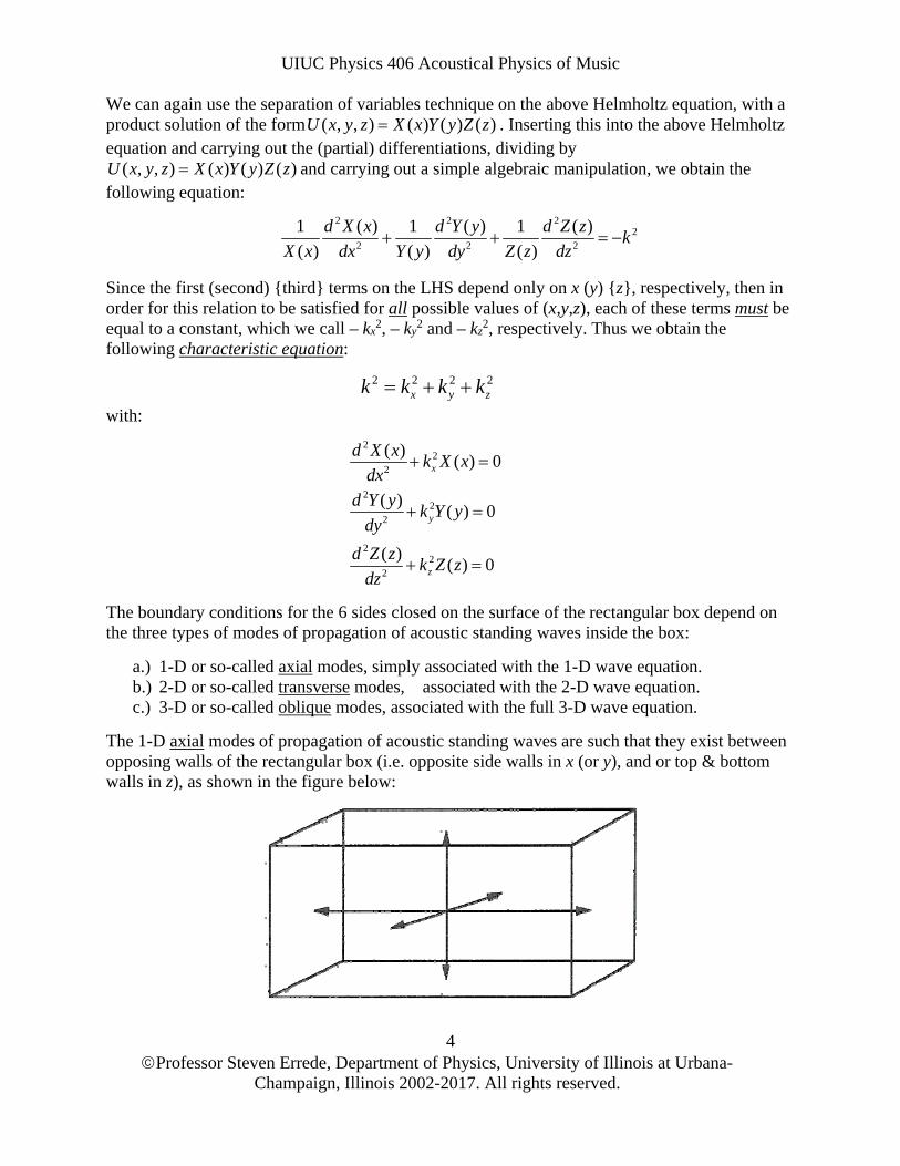
The boundary conditions for the 6 sides closed on the surface of the rectangular box depend on the three types of modes of propagation of acoustic standing waves inside the box:
a.) 1-D or so-called axial modes, simply associated with the 1-D wave equation. b.) 2-D or so-called transverse modes, associated with the 2-D wave equation. c.) 3-D or so-called oblique modes, associated with the full 3-D wave equation.
The 1-D axial modes of propagation of acoustic standing waves are such that they exist between opposing walls of the rectangular box (i.e. opposite side walls in x (or y), and or top & bottom walls in z), as shown in the figure below:
2 2 22
2 2 2
1 ( ) 1 ( ) 1 ( )
( ) ( ) ( )
d X x d Y y d Z zk
X x dx Y y dy Z z dz
2 2 2 2x y zk k k k
22
2
22
2
22
2
( )( ) 0
( )( ) 0
( )( ) 0
x
y
z
d X xk X x
dx
d Y yk Y y
dy
d Z zk Z z
dz
UIUC Physics 406 Acoustical Physics of Music
Professor Steven Errede, Department of Physics, University of Illinois at Urbana-
Champaign, Illinois 2002-2017. All rights reserved.
5
The boundary conditions on the longitudinal displacement (over-pressure) for 1-D axial modes in the x, y or z directions are such that the longitudinal displacement (over-pressure) in that direction vanishes (is maximal), respectively at the two opposing walls of the 3-D rectangular box for that mode, i.e.:
Thus, the spatial eigen-mode solutions for the longitudinal displacement (over-pressure) amplitudes associated with 1-D axial-type standing waves inside a 3-D rectangular box are respectively of the form:
and:
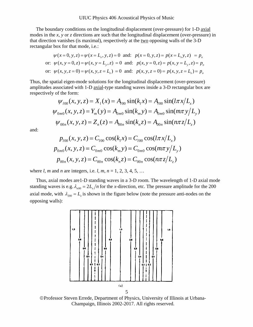
where l, m and n are integers, i.e. l, m, n = 1, 2, 3, 4, 5, …
Thus, axial modes are1-D standing waves in a 3-D room. The wavelength of 1-D axial mode standing waves is e.g. 00 2n xL n for the x-direction, etc. The pressure amplitude for the 200
axial mode, with 200 xL is shown in the figure below (note the pressure anti-nodes on the
opposing walls):
( 0, , ) ( , , ) 0 and: ( 0, , ) ( , )
or: ( , 0, ) ( , , ) 0 and: ( , 0, ) ( , , )
or: ( , , 0) ( , , ) 0 and: ( , , 0) ( , , )
x x o
y y o
z z o
x y z x L y z p x y z p x L y z p
x y z x y L z p x y z p x y L z p
x y z x y z L p x y z p x y z L p
00 00 00
0 0 0 0 0 0
00 00 00
( , , ) ( ) sin( ) sin( )
( , , ) ( ) sin( ) sin( )
( , , ) ( ) sin( ) sin( )
l l l l l x
m m m m m y
n n n n n z
x y z X x A k x A l x L
x y z Y y A k y A m y L
x y z Z z A k z A n z L
00 00 00
0 0 0 0 0 0
00 00 00
( , , ) cos( ) cos( )
( , , ) cos( ) cos( )
( , , ) cos( ) cos( )
l l l l x
m m m m y
n n n n z
p x y z C k x C l x L
p x y z C k y C m y L
p x y z C k z C n z L

UIUC Physics 406 Acoustical Physics of Music
Professor Steven Errede, Department of Physics, University of Illinois at Urbana-
Champaign, Illinois 2002-2017. All rights reserved.
6
The next type of standing waves in a room are collectively known as 2-D tangential modes, where two of the three indices are non-zero, e.g. [xyx] = [lm0], [0lm] or [l0m], with integer l,m = 1,2,3,4… These modes have 2-D type standing waves of frequency
2210 2lm x yf v l L m L , 2 21
0 2lm y zf v l L m L or 2 210 2l m x zf v l L m L
The wavelengths of 2-D tangential modes are e.g. 22
0 02 / 2lm lm x yk l L m L , etc.
For 2-D tangential modes, four of the six surfaces of the room are involved in producing a tangential standing wave. 2-D paths that can be taken for {the traveling waves associated with} such standing waves are shown in the figure below:
The boundary conditions on the longitudinal displacement (over-pressure) for 2-D tangential modes in the x, y or z directions are such that the longitudinal displacement (over-pressure) vanishes (is maximal), respectively on the four surfaces of the 3-D rectangular box for that mode, i.e.:
and:
( 0, , ) ( , , ) 0 and: ( , 0, ) ( , , ) 0
or: ( , 0, ) ( , , ) 0 and: ( , , 0) ( , , ) 0
or: ( 0, , ) ( , , ) 0 and: ( , , 0) ( , , ) 0
x y
y z
x z
x y z x L y z x y z x y L z
x y z x y L z x y z x y z L
x y z x L y z x y z x y z L
( 0, , ) ( , , ) and: ( , 0, ) ( , , )
or: ( , 0, ) ( , , ) and: ( , , 0) ( , , )
or: ( 0, , ) ( , , ) and: ( , , 0) ( , , )
x o y o
y o z o
x o z o
p x y z p x L y z p p x y z p x y L z p
p x y z p x y L z p p x y z p x y z L p
p x y z p x L y z p p x y z p x y z L p
UIUC Physics 406 Acoustical Physics of Music
Professor Steven Errede, Department of Physics, University of Illinois at Urbana-
Champaign, Illinois 2002-2017. All rights reserved.
7
The spatial eigen-mode solutions for the longitudinal displacement (over-pressure) amplitudes associated with 2-D tangential-type standing waves inside a 3-D rectangular box are respectively of the form:
and:
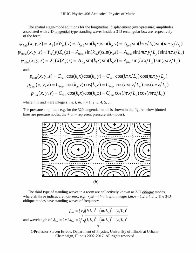
where l, m and n are integers, i.e. l, m, n = 1, 2, 3, 4, 5, …
The pressure amplitude e.g. for the 320 tangential mode is shown in the figure below (dotted lines are pressure nodes, the + or represent pressure anti-nodes):
The third type of standing waves in a room are collectively known as 3-D oblique modes, where all three indices are non-zero, e.g. [xyx] = [lmn], with integer l,m,n = 1,2,3,4,5… The 3-D oblique modes have standing waves of frequency
22 212lmm x y zf v l L m L n L
and wavelength of 22 22 / 2lmn lmn x y zk l L m L n L .
0 0 0
0 0 0
0 0 0
( , , ) ( ) ( ) sin( )sin( ) sin( )sin( )
( , , ) ( ) ( ) sin( )sin( ) sin( )sin( )
( , , ) ( ) ( ) sin( )sin( ) sin( )sin(
lm l m lm l m lm x y
mn m n mn m n mn y z
l n l n l n l n l n x
x y z X x Y y A k x k y A l x L m y L
x y z Y y Z z A k y k z A m y L n z L
x y z X x Z z A k x k z A l x L n
) zz L
0 0 0
0 0 0
0 0 0
( , , ) cos( )cos( ) cos( )cos( )
( , , ) cos( )cos( ) cos( )cos( )
( , , ) cos( )cos( ) cos( )cos( )
lm lm l m lm x y
mn mn m n mn y z
l n l n l n l n x z
p x y z C k x k y C l x L m y L
p x y z C k y k z C m y L n z L
p x y z C k x k z C l x L n z L

UIUC Physics 406 Acoustical Physics of Music
Professor Steven Errede, Department of Physics, University of Illinois at Urbana-
Champaign, Illinois 2002-2017. All rights reserved.
8
The boundary conditions on longitudinal displacement (over-pressure) amplitudes for the 3-D oblique modes in the x, y or z directions are such that the longitudinal displacement (over-pressure) amplitude vanishes (is maximal), respectively on the six surfaces of the 3-D rectangular box for that mode, i.e.:
and:
The complete eigen-mode solutions for 3-D oblique longitudinal displacement amplitude (over-pressure) standing waves inside a rectangular box are thus respectively given by:
and:
where l, m and n are integers, i.e. l, m, n = 1, 2, 3, 4, 5, …
The eigen-frequencies, eigen-wavelengths and eigen-energies associated with 1-D axial, 2-D tangential and 3-D oblique modes of standing waves inside a 3-D rectangular box via the “generic formulas:
( , , , ) sin( ) sin( ) sin( )
( , , , ) sin( )sin( )sin( )
lmn lmn
lmn lmn
i tlmn lmn l m n
i tlmn lmn x y z
x y z t A k x k y k z e
x y z t A l x L m y L n z L e
22 212
22 2
22 22 2 2 2 2 2 2 21 1, , , , , , , , , , , ,4 4
2 / 2
, , 0,1,
lmm x y z
lmn lmn x y z
l m n l m n l m n l m n l m n l m n x y z
f v l L m L n L
k l L m L n L
E M A Mf A v MA l L m L n L
l m n
( 0, , ) ( , , ) 0 and: ( , 0, ) ( , , ) 0
and: ( , , 0) ( , , ) 0
x y
z
x y z x L y z x y z x y L z
x y z x y z L
( 0, , ) ( , , ) and: ( , 0, ) ( , , )
and: ( , , 0) ( , , )
x o y o
z o
p x y z p x L y z p p x y z p x y L z p
p x y z p x y z L p
( , , , ) cos( ) cos( ) cos( )
( , , , ) cos( ) cos( ) cos( )
lmn lmn
lmn lmn
i tlmn lmn l m n
i tlmn lmn x y z
p x y z t C k x k y k z e
p x y z t C l x L m y L n z L e

UIUC Physics 406 Acoustical Physics of Music
Professor Steven Errede, Department of Physics, University of Illinois at Urbana-
Champaign, Illinois 2002-2017. All rights reserved.
9
For the special case of a cubical box with all sides Lx = Ly = Lz = L, then the eigen-frequencies, eigen-wavelengths, eigen-energies, etc. are:
Here again, as we saw in e.g. the 2-D case for standing waves on a rectangular square membrane, degeneracies will exist. We summarize this for the first few modes of longitudinal standing waves in a cubical box in the table below.
[l,m,n] Mode Degeneracy Mode Type [100,010,001] 3 1-D Axial [101,011,110] 3 2-D Transverse
[111] 1 3-D Oblique [200,020,002] 3 1-D Axial
[201,210,021,012,102,120] 6 2-D Transverse [211,121,112] 3 3-D Oblique
Thus, the degeneracies associated with a cubical-shaped room imply that e.g. a cubical room will be more problematic in terms of room resonances and acoustic feedback than for a rectangular-shaped room, where {Lx Ly Lz}. This can be seen from the so-called density of states for 3-D standing waves in a cubical vs. rectangular room, as shown in the figure below for two equal volume rooms, one cubical, the other rectangular, the latter with L:W:H ratio 3:2:1:
2 2 212
2 2 2
22 2 2 2 2 2 2 2 2 21 1
4 4
/ 2 / 2 /
2 / 2
, , 0,1,
lmn lmn lmn lmn
lmn lmn
lmn lmn lmn lmn lmn lmn
vf vk v l m n
L
k L l m n
vE M A Mf A MA l m n
L
l m n
UIUC Physics 406 Acoustical Physics of Music
Professor Steven Errede, Department of Physics, University of Illinois at Urbana-
Champaign, Illinois 2002-2017. All rights reserved.
10
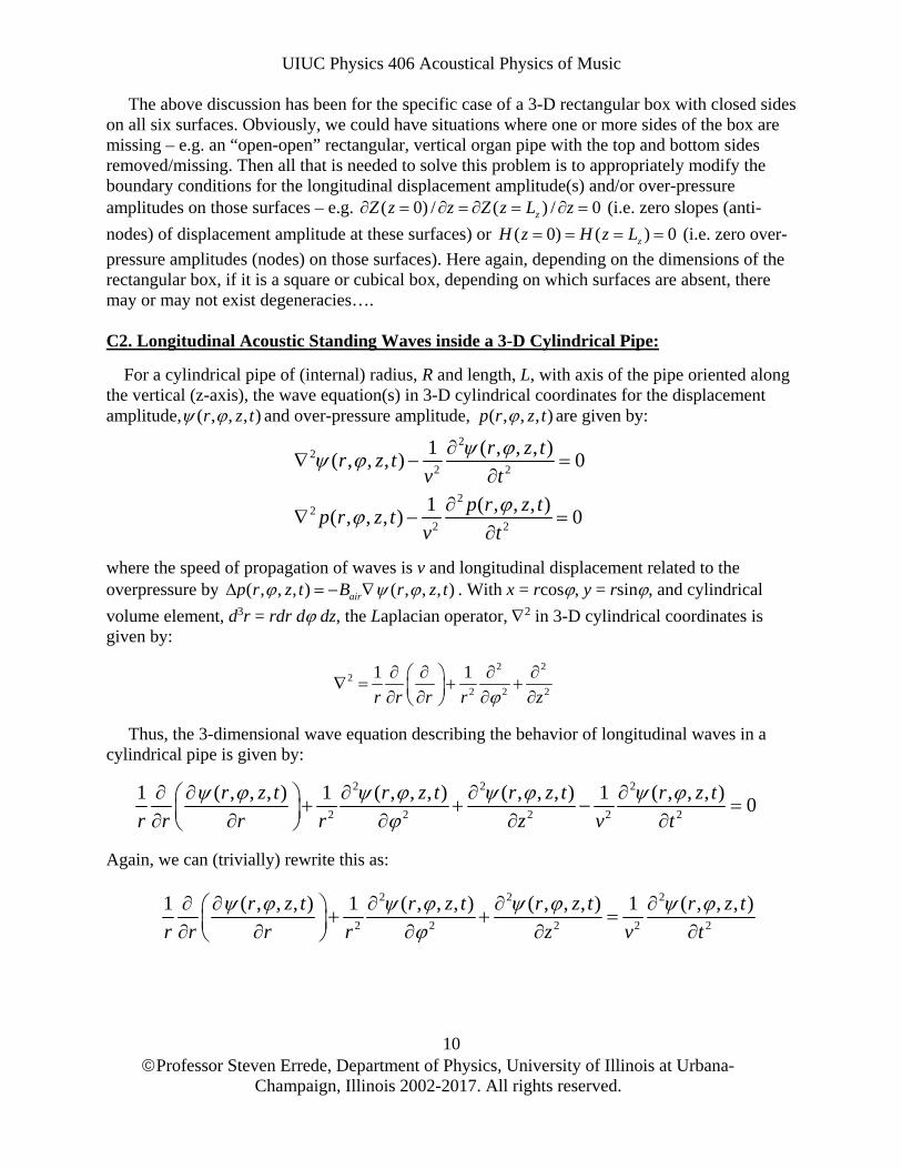
The above discussion has been for the specific case of a 3-D rectangular box with closed sides on all six surfaces. Obviously, we could have situations where one or more sides of the box are missing – e.g. an “open-open” rectangular, vertical organ pipe with the top and bottom sides removed/missing. Then all that is needed to solve this problem is to appropriately modify the boundary conditions for the longitudinal displacement amplitude(s) and/or over-pressure amplitudes on those surfaces – e.g. ( 0) / ( ) / 0zZ z z Z z L z (i.e. zero slopes (anti-
nodes) of displacement amplitude at these surfaces) or ( 0) ( ) 0zH z H z L (i.e. zero over-
pressure amplitudes (nodes) on those surfaces). Here again, depending on the dimensions of the rectangular box, if it is a square or cubical box, depending on which surfaces are absent, there may or may not exist degeneracies…. C2. Longitudinal Acoustic Standing Waves inside a 3-D Cylindrical Pipe:
For a cylindrical pipe of (internal) radius, R and length, L, with axis of the pipe oriented along the vertical (z-axis), the wave equation(s) in 3-D cylindrical coordinates for the displacement amplitude, ( , , , )r z t and over-pressure amplitude, ( , , , )p r z t are given by:
where the speed of propagation of waves is v and longitudinal displacement related to the overpressure by ( , , , ) ( , , , )airp r z t B r z t . With x = rcos, y = rsin, and cylindrical
volume element, d3r = rdr d dz, the Laplacian operator, 2 in 3-D cylindrical coordinates is given by:
Thus, the 3-dimensional wave equation describing the behavior of longitudinal waves in a cylindrical pipe is given by:
Again, we can (trivially) rewrite this as:
22
2 2
22
2 2
1 ( , , , )( , , , ) 0
1 ( , , , )( , , , ) 0
r z tr z t
v t
p r z tp r z t
v t
2 22
2 2 2
1 1
r r r r z
2 2 2
2 2 2 2 2
1 ( , , , ) 1 ( , , , ) ( , , , ) 1 ( , , , )0
r z t r z t r z t r z t
r r r r z v t
2 2 2
2 2 2 2 2
1 ( , , , ) 1 ( , , , ) ( , , , ) 1 ( , , , )r z t r z t r z t r z t
r r r r z v t
UIUC Physics 406 Acoustical Physics of Music
Professor Steven Errede, Department of Physics, University of Illinois at Urbana-
Champaign, Illinois 2002-2017. All rights reserved.
11
Notice again that the LHS (RHS) contains only spatial-dependent (time-dependent) functions, respectively. Thus, we again can use the technique of separation of variables, with
( , , , ) ( , , ) ( )r z t U r z T t where ( , , )U r z contains only spatially r-, - and z-dependent terms and ( )T t contains only the time-dependent term.
Again, we have the relation v = f = (/2)(2/k) = /k; thus vk = . We again obtain a separation constant of – k2, and, after some simple algebraic manipulations, obtain the following two linear, homogeneous differential equations:
We can again use the separation of variables technique on the above Helmholtz equation, however, first we will consciously separate out the z-dependence from the (r,) portion, using a product solution of the form ( , , ) ( , ) ( )U r z V r Z z . Inserting this into the above Helmholtz equation and carrying out the (partial) differentiations, dividing by ( , , ) ( , ) ( )U r z V r Z z and carrying out a simple algebraic manipulation, we obtain the following two equations:
where 2zk is the separation constant for this product solution. We can rewrite each of these two
equations as:
The second wave equation, that for Z(z) we’ve seen before (déjà vu!) e.g. for the four boundary condition cases associated with one-dimensional longitudinal standing waves in closed-closed, open-open, closed-open and open-closed organ pipes of length, L. Thus, we immediately know what the mathematical form of the longitudinal standing wave eigen-solutions are for Z(z), depending on which of the four boundary conditions are imposed at Z(z=0) and Z(z=L):
2 22
2 2 2
22
2
1 ( , , ) 1 ( , , ) ( , , )( , , ) 0
( )( ) 0
U r z U r z U r zk U r z
r r r r z
d T tT t
dt
2
2 22 2
22
2
1 1 ( , ) 1 1 ( , )0
( , ) ( , )
1 ( )0
( )
z
z
V r V rr k k
V r r r r V r r
d Z zk
Z z dz
2
2 22 2
22
2
1 ( , ) 1 ( , )( , ) 0
( )( ) 0
z
z
V r V rr k k V r
r r r r
d Z zk Z z
dz

UIUC Physics 406 Acoustical Physics of Music
Professor Steven Errede, Department of Physics, University of Illinois at Urbana-
Champaign, Illinois 2002-2017. All rights reserved.
12
A.) Closed-Closed Ends (Dirichlet BC’s):
B.) Open-Open Ends (Neumann BC’s):
C.) Closed-Open Ends (Cauchy BC’s):
D.) Open-Closed Ends (Cauchy BC’s):
Thus, we see that the Z(z)-dependent behavior associated with longitudinal standing waves in a 3-D cylindrical pipe of radius, R and length, L is precisely the same as that associated with an “idealized” one-dimensional organ pipe of the same length, L. Note that these solutions are also relevant e.g. for a 3-D cylindrical “singing rod” of radius, R and length, L made of an elastic solid, such as aluminum.
We now turn our attention to finding the eigen-solutions, etc. associated with solving the ( , )V r equation. We again try a product solution of the form ( , ) ( ) ( )V r R r . Again, after some simple algebraic manipulations, we obtain the following:
Note again that the LHS (RHS) of this relation depends only on r (), respectively, thus:
Again, the separation constant, m2 arises because we insist upon physically-sensible, single-valued solutions of the ( ) -equation, namely that ( 0) ( 2 ) ( 2 );m with m
= 0, 1, 2, 3, 4, 5, … Thus, the eigen-solutions, ( )m of the ( ) -equation:
are again one of two equivalent forms:
( 0) ( ) 0; ( ) ~ sin( ) sin(2 / ); / ; 1, 2, 3, 4, 5,...C Cn z z nZ z Z z L Z z k z nz L k k n L n
( 0) ( )0; ( ) ~ cos( ) cos(2 / ); / ; 1, 2, 3, 4, 5,...O O
n z z n
dZ z dZ z LZ z k z nz L k k n L n
dz dz
( )( 0) 0; ( ) ~ sin( ) sin(4 / ); / ; 1, 3, 5, 7, 9,...C O
n z z n
dZ z LZ z Z z k z nz L k k n L n
dz
( 0)( ) 0; ( ) ~ cos( ) cos(4 / ); / ; 1, , , , ,...O C
n z z n
dZ zZ z L Z z k z nz L k k n L n
dz
2
2 2 2 22
1 ( ) 1 ( )
( ) ( )z
d dR r dr r k k r m
R r dr dr d
2 2 2 2
22
2
( )( ) 0
( )( ) 0
z
d dR rr r k k r m R r
dr dr
dm
d
22
2
( )( ) 0m
m
dm
d
2 2
1
( ) cos sin
1 1 1 1 1
( ) tan
0, 1, 2, 3,....
m
m m m
m m m m
i mm m m m
m m
e
m
UIUC Physics 406 Acoustical Physics of Music
Professor Steven Errede, Department of Physics, University of Illinois at Urbana-
Champaign, Illinois 2002-2017. All rights reserved.
13
Now for the radial equation, note that 2 2 2z rk k k or 2 2 2
r zk k k . Then the radial equation
becomes:
Again, this linear, homogeneous, 2nd-order differential equation is the Bessel equation, the allowed eigen-solutions for a displacement amplitude node at r = R i.e. R(r = R)=0 we have already discussed above for the 2-D circular membrane! They are of the form:
However, again on physical grounds, the Bessel functions of the 2nd kind must be excluded because they are singular at the origin, i.e. r = 0. Hence all coefficients, Bm = 0 for all m. Thus for the physically-allowed radial eigen-function solutions, we have only:
The radial boundary condition for longitudinal standing waves in a rigid, 3-D circular pipe at r = R is Rm(r=R) = 0, i.e. the zeroes associated with Jm(x=krR), i.e. Jm(x=krR) = 0, precisely as we found for the radial eigen-modes in the 2-D circular membrane case!
Since x = krR, then kr = x/R and noting that again, for this 2-dimensional longitudinal standing wave eigen-value problem in the r- plane, we need to have two indices, m and j to denote the radial eigen-wavenumbers, i.e. , , /m j m jk x R , where the first (second) index, m = 0, 1, 2, 3,…
(j = 1, 2, 3, 4, …) denotes the order # (zero #) of the ordinary Bessel function of the first kind, ,( )m m jJ k R respectively.
For the eigen-solutions associated with standing waves in a 3-D circular pipe, the characteristic equation becomes:
The eigen-frequencies, eigen-wavelengths, eigen-energies, etc. are given by:
2 2 2( )( ) 0r
d dR rr r k r m R r
dr dr
( ) ( ) ( )m m m r m m rR r A J k r B Y k r
( ) ( )m m m rR r A J k r
2 2 2 2 2 2, , ,r z m j n m j nk k k k k k
2 2 2 2, , , , , , , , , , , ,
2 2, , ,
, ,
2 2 /
2 ;
/ , 0,1,2,3, .... 1, 2,3,4, ....
2 / 1,2,3,4, .... 4 / 1,3,5,7,
m j n m j n m j n m j n m j n m j n m j n
m j n m j n
m j m j
n n
vk v k k f v k k v
k k
k x R m j
k n L n or k n L n
2 2 2 2 2 2 2 2 21 1
, , , , , , , , , , , , ,4 4
....
m j n air m j n m j n air m j n m j n air m j n m j nE M A M f A M v A k k

UIUC Physics 406 Acoustical Physics of Music
Professor Steven Errede, Department of Physics, University of Illinois at Urbana-
Champaign, Illinois 2002-2017. All rights reserved.
14
The eigen-mode solutions of the associated temporal wave equation for longitudinal standing waves inside a 3-D circular pipe are of the following equivalent form(s):
The complete eigen-mode solutions for longitudinal displacement amplitude standing waves inside a 3-D cylindrical pipe are thus given e.g. by:
Thus, we see that the eigen-solutions, etc. for longitudinal standing waves in a 3-D cylindrical pipe are intimately related to those associated with the simpler model of a 1-D organ pipe! The following figure shows the (over-)pressure and transverse air-flow in a cross-section of a cylindrical pipe for the three lowest standing wave modes after the fundamental.
, , , ,
, , , , , , , , , ,
2 2, , , , , , , ,
, , , , , ,
, , , , , ,
, , , , 2
, ,
( ) sin cos
1 1 1 1 1
( ) sin
( ) cos
( ) m j n m j n
m j n m j n m j n m j n m j n
m j n m j n m j n m j n
m j n m j n m j n
m j n m j n m j n
m j n m j n
i t
m j n
T t b t c t
b c b c
T t t
T t t
T t e
, , , ,
, , , ,
, , , , ,
, , , , , , , , , , , , ,
( , , , ) ( ) ( ) ( ) ( )
( , , , ) ( )
( , , , ) ( ) cos sin cos sin cos sin
m j n m j nm n n
m j n m j m n m n
i ti m i k zm j n m j n m m j
m j n m j n m m j m m m n m n m j n m j n m j n m j n
r z t R r Z z T t
r z t A J k r e e e
r z t A J k r m m k z k z b t c t

UIUC Physics 406 Acoustical Physics of Music
Professor Steven Errede, Department of Physics, University of Illinois at Urbana-
Champaign, Illinois 2002-2017. All rights reserved.
15
The figure shown below shows a side view of the acoustic flow patterns and pressure maxima/minima for higher modes in a cylindrical pipe.
The so-called critical frequency (also known as the cutoff frequency), , , , ,Critm j n m j nvk .
For modal frequencies less than this, , ,m j nk is imaginary, and this particular mode is exponentially
attenuated – it is known as an evanescent wave.

UIUC Physics 406 Acoustical Physics of Music
Professor Steven Errede, Department of Physics, University of Illinois at Urbana-
Champaign, Illinois 2002-2017. All rights reserved.
16
C3. Longitudinal Acoustic Standing Waves inside a 3-D Sphere:
Finally, the last system we consider here in this set of lecture notes is longitudinal standing waves inside a 3-D sphere of radius, R. The wave equation(s) in 3-D spherical polar coordinates for the displacement amplitude, ( , , , )r t and over-pressure amplitude, ( , , , )p r t are given by:
where the speed of propagation of waves is v and longitudinal displacement related to the overpressure by ( , , , ) ( , , , )airp r t B r t . With x = rsincos, y = rsinsin,
z = rcos, 2 2 2r x y z , cos = z/r, tan = y/x and spherical volume element,
d3r = r2dr d = r2dr dcos d = r2dr sin d d, the Laplacian operator, 2 in 3-D spherical polar coordinates is given by:
Thus, the 3-dimensional wave equation describing the behavior of longitudinal waves in a cylindrical pipe is given by:
Again, we can (trivially) rewrite this as:
Notice again that the LHS (RHS) contains only spatial-dependent (time-dependent) functions, respectively. Thus, we again can use the technique of separation of variables, with
( , , , ) ( , , ) ( )r t U r T t where ( , , )U r contains only spatially r-, - and -dependent terms and ( )T t contains only the time-dependent term.
Again, we have the relation v = f = (/2)(2/k) = /k; thus vk = . We again obtain a separation constant of – k2, and, after some simple algebraic manipulations, obtain the following two linear, homogeneous differential equations:
22
2 2
22
2 2
1 ( , , , )( , , , ) 0
1 ( , , , )( , , , ) 0
r tr t
v t
p r tp r t
v t
22 2
2 2 2 2 2
1 1 1sin
sin sinr
r r r r r
2 22
2 2 2 2 2 2 2
1 1 1 1 ( , , , )sin ( , , , ) 0
sin sin
r tr r t
r r r r r v t
2 22
2 2 2 2 2 2 2
1 1 1 1 ( , , , )sin ( , , , )
sin sin
r tr r t
r r r r r v t
22 2
2 2 2 2 2
22
2
1 1 1sin ( , , ) ( , , ) 0
sin sin
( )( ) 0
r U r k U rr r r r r
d T tT t
dt

UIUC Physics 406 Acoustical Physics of Music
Professor Steven Errede, Department of Physics, University of Illinois at Urbana-
Champaign, Illinois 2002-2017. All rights reserved.
17
We can again use the separation of variables technique on the above Helmholtz equation, however, first we will consciously separate out the angular (,)-dependence from the radial, r-dependent portion, using a product solution of the form ( , , ) ( ) ( , )U r R r Y . Inserting this into the above Helmholtz equation and carrying out the (partial) differentiations, dividing by
( , , ) ( ) ( , )U r R r Y and carrying out a simple algebraic manipulation, we obtain the following two equations:
where is the separation constant for this product solution. We can rewrite each of these two equations as:
We can again use the separation of variables technique on the angular equation, writing the angular solution, ( , )Y as a product solution of the form ( , ) ( ) ( )Y . Inserting this
into the above equation, multiplying through by sin2, carrying out the partial derivatives and some simple algebraic manipulations, we obtain the following two equations:
which have a separation constant, m2. Again, these two equations can be rewritten as:
The second equation, involving the azimuthal angle, is the usual one we have been dealing with. The separation constant, m2 arises because we insist upon physically-sensible, single-valued solutions of the ( ) -equation, i.e. ( 0) ( 2 ) ( 2 );m
with m = 0, 1, 2, 3, 4, 5, … and with corresponding eigen-solutions of the form ( )( ) ~ mi m
m e .
2
2 2
2 2 2
1 1 ( , ) 1 ( , )sin
( , ) sin sin
1 ( )( )
( )
Y Y
Y
d dR rr k r R r
R r dr dr
2
2 2
2 2 2
1 ( , ) 1 ( , )sin ( , ) 0
sin sin
( )( ) 0
Y YY
d dR rr k r R r
dr dr
2 2
22
2
1 ( )sin sin sin ( )
( )
1 ( )
( )
d dm
d d
dm
d
2 2
22
2
( )sin sin sin ( ) 0
( )( ) 0
d dm
d d
dm
d

UIUC Physics 406 Acoustical Physics of Music
Professor Steven Errede, Department of Physics, University of Illinois at Urbana-
Champaign, Illinois 2002-2017. All rights reserved.
18
The first equation, involving the polar angle, is known as the Associated Legendre equation. Skipping some ~ tedious derivational details, the separation constant,
( 1); 0,1, 2, 3, 4, .... with the additional constraint that | |m , with m = 0, 1, 2,
3, 4, 5, … For = integers, the most general form of the eigen-solutions for the associated Legendre equation are linear combination of associated Legendre polynomials, ( )mP x and
( )mQ x of the first and second kind, respectively, with cosx , i.e.
If the poles (i.e. = 0 and = ) are excluded from the physical problem (corresponding to x = 1), then both of the 1st and 2nd kind associated Legendre polynomials must be included. However, if the poles are included in the physical problem, then the associated Legendre polynomials of the 2nd kind, ( )mQ x must be excluded, because they are singular at x = 1. For our
problem of standing waves inside a sphere of radius, R, the poles at = 0 and = are included and hence the associated Legendre polynomials of the 2nd kind, ( )mQ x must be
excluded, hence we require all , 1ma and all , 0mb .
For integer values of , the associated Legendre polynomials of the first kind, ( )mP x are such
that ( ) ( )m mP x P x . With cosx these functions are products of | |sin m and are polynomials
of degree ( | |); | |m m in cosx . These functions are even if ( | |)m is even, and odd, if ( | |)m is odd.
The angular eigen-solutions for the (,) product solution are thus of the form:
Note that the ( , )mY are normalized, orthogonal functions known as spherical harmonics.
Appropriate linear combinations of the ( , )mY can precisely describe any arbitrary (but well-
behaved, non-singular) angular function ( , )f everywhere on the unit sphere (r = R = 1), i.e.
| |2 ( )2 1 ( | |)!
( , ) ( ) ( ) ( , ) ( 1) ( )4 ( | |)!
m mm m i mm
Y Y P em
,0 ,
| |
( , ) ( , )mm
mm
f a Y
, , ,( ) ( ) ( )m mm m mx a P x b Q x
UIUC Physics 406 Acoustical Physics of Music
Professor Steven Errede, Department of Physics, University of Illinois at Urbana-
Champaign, Illinois 2002-2017. All rights reserved.
19
The first few spherical harmonics are listed in the table below.
0 1 2
0m 00
1( , )
4Y
0
1
3( , ) cos
4Y
20
2
5 3cos 1( , )
4 2Y
1m
11
3( , ) sin
8iY e
1
2
5( , ) 3sin cos
24iY e
2m
2 2 22
5( , ) 3sin
96iY e
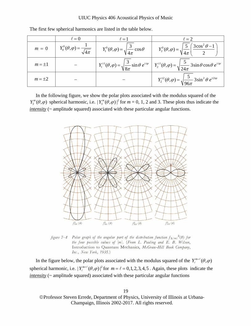
In the following figure, we show the polar plots associated with the modulus squared of the
3 ( , )mY spherical harmonic, i.e. 23| ( , ) |mY for m = 0, 1, 2 and 3. These plots thus indicate the
intensity (~ amplitude squared) associated with these particular angular functions.
In the figure below, the polar plots associated with the modulus squared of the ( , )mY
spherical harmonic, i.e. 2| ( , ) |mY for 0,1,2,3,4,5m . Again, these plots indicate the
intensity (~ amplitude squared) associated with these particular angular functions

UIUC Physics 406 Acoustical Physics of Music
Professor Steven Errede, Department of Physics, University of Illinois at Urbana-
Champaign, Illinois 2002-2017. All rights reserved.
20

UIUC Physics 406 Acoustical Physics of Music
Professor Steven Errede, Department of Physics, University of Illinois at Urbana-
Champaign, Illinois 2002-2017. All rights reserved.
21
We now turn our attention to solving and finding the eigen-solutions associated with the radial equation:
If we make a change of variables, ( ) ( ) /R r u r r then inserting this into the above equation, carrying out the differentiation, after some algebraic manipulations, we obtain:
Which again, is Bessel’s equation with x kr and 12" "m . Thus, the most general form of
the radial eigen-solutions is:
By convention, we define the so-called spherical Bessel functions of first and second kind, of order as:
It can be shown that:
The analytic form e.g. of the first two 0,1 spherical Bessel functions are thus:
0
sin xj x
x and 0
cos xy x
x
1 2
sin cosx xj x
x x and 1 2
cos sinx xy x
x x
Note that 0
sin xj x
x is sometimes also called the sinc function, i.e. 0
sin xj x sinc x
x
2 22 2
1 ( ) ( 1)( ) 0
d dR rr k R r
r dr dr r
22 12 2
2 2
( )( ) 1 ( )( ) 0
d u r du rk u r
dr r dr r
1 12 2
1 1 12 2 2
( ) ( )( )
J kr Y krR r A B
r r
1 12 2
( ) ( ) ( ) ( )2 2
j x J x y x Y xx x
1 sin 1 cos( ) ( ) ( ) ( )
d x d xj x x y x x
x dx x x dx x
UIUC Physics 406 Acoustical Physics of Music
Professor Steven Errede, Department of Physics, University of Illinois at Urbana-
Champaign, Illinois 2002-2017. All rights reserved.
22
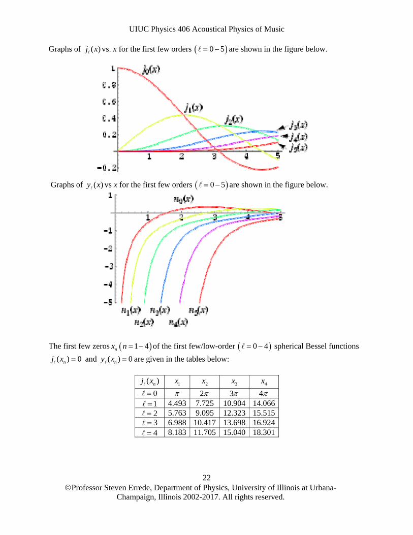
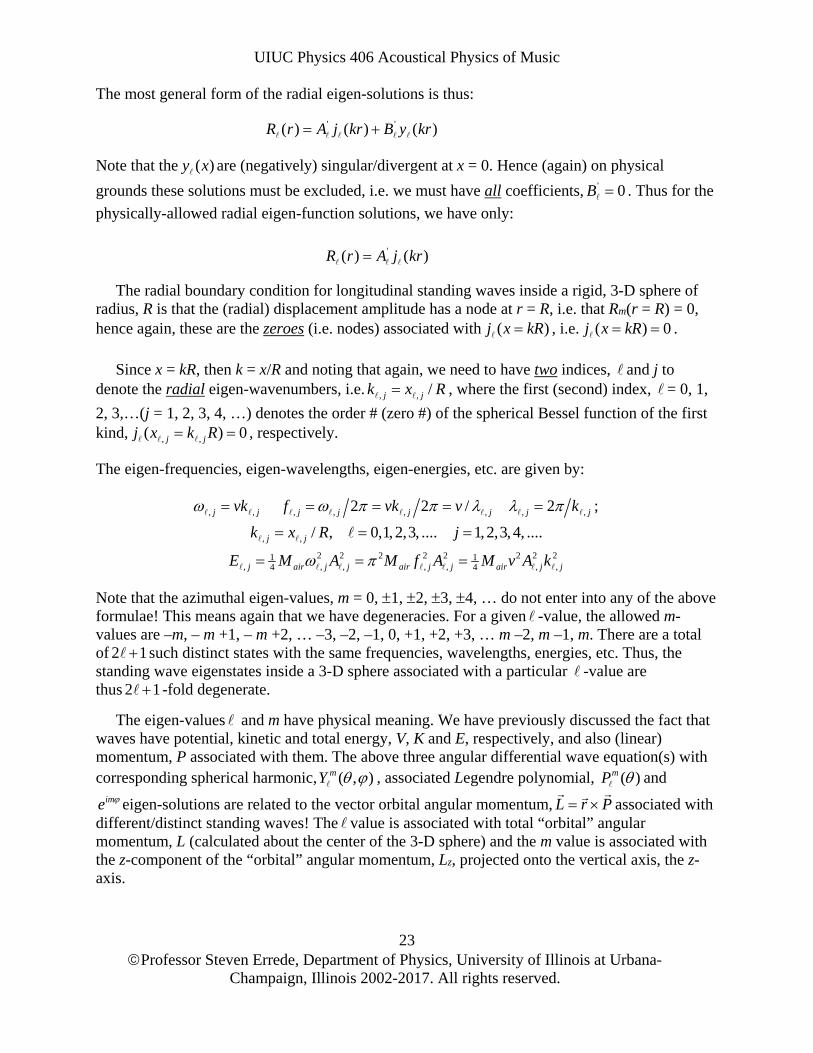
Graphs of ( )j x vs. x for the first few orders 0 5 are shown in the figure below.
Graphs of ( )y x vs x for the first few orders 0 5 are shown in the figure below.
The first few zeros nx 1 4n of the first few/low-order 0 4 spherical Bessel functions
( ) 0nj x and ( ) 0ny x are given in the tables below:
( )nj x 1x 2x 3x 4x
0 2 3 4 1 4.493 7.725 10.904 14.066 2 5.763 9.095 12.323 15.515 3 6.988 10.417 13.698 16.924 4 8.183 11.705 15.040 18.301
UIUC Physics 406 Acoustical Physics of Music
Professor Steven Errede, Department of Physics, University of Illinois at Urbana-
Champaign, Illinois 2002-2017. All rights reserved.
23
The most general form of the radial eigen-solutions is thus:
Note that the ( )y x are (negatively) singular/divergent at x = 0. Hence (again) on physical
grounds these solutions must be excluded, i.e. we must have all coefficients, ' 0B . Thus for the
physically-allowed radial eigen-function solutions, we have only:
The radial boundary condition for longitudinal standing waves inside a rigid, 3-D sphere of radius, R is that the (radial) displacement amplitude has a node at r = R, i.e. that Rm(r = R) = 0, hence again, these are the zeroes (i.e. nodes) associated with ( )j x kR , i.e. ( ) 0j x kR .
Since x = kR, then k = x/R and noting that again, we need to have two indices, and j to denote the radial eigen-wavenumbers, i.e. , , /j jk x R , where the first (second) index, = 0, 1,
2, 3,…(j = 1, 2, 3, 4, …) denotes the order # (zero #) of the spherical Bessel function of the first kind, , ,( ) 0j jj x k R , respectively.
The eigen-frequencies, eigen-wavelengths, eigen-energies, etc. are given by:
Note that the azimuthal eigen-values, m = 0, 1, 2, 3, 4, … do not enter into any of the above formulae! This means again that we have degeneracies. For a given -value, the allowed m-values are –m, – m +1, – m +2, … –3, –2, –1, 0, +1, +2, +3, … m –2, m –1, m. There are a total of 2 1 such distinct states with the same frequencies, wavelengths, energies, etc. Thus, the standing wave eigenstates inside a 3-D sphere associated with a particular -value are thus 2 1 -fold degenerate.
The eigen-values and m have physical meaning. We have previously discussed the fact that waves have potential, kinetic and total energy, V, K and E, respectively, and also (linear) momentum, P associated with them. The above three angular differential wave equation(s) with corresponding spherical harmonic, ( , )mY , associated Legendre polynomial, ( )mP and
ime eigen-solutions are related to the vector orbital angular momentum, L r P
associated with different/distinct standing waves! The value is associated with total “orbital” angular momentum, L (calculated about the center of the 3-D sphere) and the m value is associated with the z-component of the “orbital” angular momentum, Lz, projected onto the vertical axis, the z-axis.
, , , , , , , ,
, ,
2 2 2 2 2 2 2 21 1, , , , , , ,4 4
2 2 / 2 ;
/ , 0,1, 2,3, .... 1, 2,3, 4, ....
j j j j j j j j
j j
j air j j air j j air j j
vk f vk v k
k x R j
E M A M f A M v A k
' '( ) ( ) ( )R r A j kr B y kr
'( ) ( )R r A j kr
UIUC Physics 406 Acoustical Physics of Music
Professor Steven Errede, Department of Physics, University of Illinois at Urbana-
Champaign, Illinois 2002-2017. All rights reserved.
24
Glossed over in the details of the derivation of the separation constant, ( 1) associated with the angular differential equation(s) for the spherical harmonics/associated Legendre polynomials was the fact that the total angular momentum, L is not in fact an eigen-state, however, the square of the total angular momentum, L2 is an eigen-state, as is the z-component of the angular momentum, Lz. In other words, both L2 and Lz are each what is known as an operator, such that:
2 2, , 0 , ,( , , , ) ( 1) ( , , , )j m j mL r t L r t and , , 0 , ,( , , , ) ( , , , )z j m j mL r t mL r t
where L0 is the smallest unit (“quanta”) of angular momentum associated with the physical problem (MKS units: kg-m2/sec).
The eigen-states with 0 have zero total angular momentum and thus have spherically symmetric eigen-solutions. Eigen-states with increasingly higher -values have increasingly higher orbital angular momentum associated with them and thus are increasingly non-spherically symmetric.
The eigen-mode solutions of the associated temporal wave equation for longitudinal standing waves inside a 3-D sphere of radius, R are of the following equivalent form(s):
The complete eigen-mode solutions for longitudinal displacement amplitude standing waves inside a 3-D sphere of radius, R are thus given e.g. by:
Note that the above formalism is also relevant for longitudinal standing waves in a 3-D sphere of radius, R e.g. made of an elastic solid, and/or sound waves in e.g. a water drop. However, the radial boundary condition for these would instead be ( ) / 0dR r R dr , i.e. zero slope of the
radial functions – i.e. the anti-nodes of the spherical Bessel functions of order, , the ( )j x kR .
, ,
, , , , ,
2 2, , , ,
, , ,
, , ,
, , 2
,
( ) sin cos
1 1 1 1 1
( ) sin
( ) cos
( ) j j
j j j j j
j j j j
j j j
j j j
j j
i t
j
T t b t c t
b c b c
T t t
T t t
T t e
, ,
, , , ,
, , , , ,
, , , , , , , , ,
( , , , ) ( ) ( , ) ( )
( , , , ) ( ) ( , )
( , , , ) ( ) ( , ) cos sin
j j
mj m j j
i tmj m j m j
mj m j m j j j j j
r t R r Y T t
r t A j k r Y e
r t A j k r Y b t c t
UIUC Physics 406 Acoustical Physics of Music
Professor Steven Errede, Department of Physics, University of Illinois at Urbana-
Champaign, Illinois 2002-2017. All rights reserved.
25
Despite the fact that there aren’t many musical instruments that are spherical in shape, the eigen-solutions, eigen-frequencies, eigen-energies, etc. associated with standing waves inside a 3-D sphere do indeed have many interesting applications – e.g. sound waves in the interior of (all kinds of) stars, surface waves propagating near the star’s surface (where the origin, r = 0 is excluded), e.g. sound waves and radio waves in our earth’s ionosphere (again where the origin, r = 0 is excluded), gravitational waves in the early universe, as well as sound waves (propagating in the plasma) of the early universe, during ~ the first 350,000 – 400,000 years after the big bang!

UIUC Physics 406 Acoustical Physics of Music
Professor Steven Errede, Department of Physics, University of Illinois at Urbana-
Champaign, Illinois 2002-2017. All rights reserved.
26
Legal Disclaimer and Copyright Notice:
Legal Disclaimer:
The author specifically disclaims legal responsibility for any loss of profit, or any consequential, incidental, and/or other damages resulting from the mis-use of information contained in this document. The author has made every effort possible to ensure that the information contained in this document is factually and technically accurate and correct.
Copyright Notice:
The contents of this document are protected under both United States of America and International Copyright Laws. No portion of this document may be reproduced in any manner for commercial use without prior written permission from the author of this document. The author grants permission for the use of information contained in this document for private, non-commercial purposes only.