chapter 12 monitoring drought using the standardized

University of Nebraska - LincolnDigitalCommons@University of Nebraska - Lincoln

Drought Mitigation Center Faculty Publications Drought -- National Drought Mitigation Center

2000

Chapter 12 Monitoring Drought Using theStandardized Precipitation IndexMichael J. HayesUniversity of Nebraska-Lincoln, [email protected]

Mark D. SvobodaUniversity of Nebraska - Lincoln, [email protected]

Donald A. WilhiteUniversity of Nebraska - Lincoln, [email protected]

Follow this and additional works at: http://digitalcommons.unl.edu/droughtfacpub

This Article is brought to you for free and open access by the Drought -- National Drought Mitigation Center at DigitalCommons@University ofNebraska - Lincoln. It has been accepted for inclusion in Drought Mitigation Center Faculty Publications by an authorized administrator ofDigitalCommons@University of Nebraska - Lincoln.

Hayes, Michael J.; Svoboda, Mark D.; and Wilhite, Donald A., "Chapter 12 Monitoring Drought Using the Standardized PrecipitationIndex" (2000). Drought Mitigation Center Faculty Publications. 70.http://digitalcommons.unl.edu/droughtfacpub/70

http://digitalcommons.unl.edu?utm_source=digitalcommons.unl.edu%2Fdroughtfacpub%2F70&utm_medium=PDF&utm_campaign=PDFCoverPages

http://digitalcommons.unl.edu/droughtfacpub?utm_source=digitalcommons.unl.edu%2Fdroughtfacpub%2F70&utm_medium=PDF&utm_campaign=PDFCoverPages

http://digitalcommons.unl.edu/drought?utm_source=digitalcommons.unl.edu%2Fdroughtfacpub%2F70&utm_medium=PDF&utm_campaign=PDFCoverPages

http://digitalcommons.unl.edu/droughtfacpub?utm_source=digitalcommons.unl.edu%2Fdroughtfacpub%2F70&utm_medium=PDF&utm_campaign=PDFCoverPages

http://digitalcommons.unl.edu/droughtfacpub/70?utm_source=digitalcommons.unl.edu%2Fdroughtfacpub%2F70&utm_medium=PDF&utm_campaign=PDFCoverPages

Published in Drought: A Global Assessment, Vol. I, edited by Donald A. Wilhite, chap. 12, pp. 168–180 (London: Routledge, 2000). Copyright © 2000 Donald A. Wilhite for the selection and editorial matter; individual chapters, the contributors. Chapter 12

Monitoring Drought Using the Standardized Precipitation Index Michael Hayes, Mark Svoboda, and Donald A. Wilhite

Introduction Because drought is so difficult to define, detect, and measure, researchers have been striv-ing to develop indices to accomplish these tasks. The importance and historical develop-ment of drought indices for monitoring drought is emphasized in the chapters by Redmond (chapter 10) and Heim (chapter 11). The goal of a drought index is to provide a simple, quantitative assessment of three drought characteristics: intensity, duration, and spatial extent. A drought index should also provide a historical reference that can be used to compare current conditions with past conditions.

In 1993, researchers at Colorado State University developed a new drought index, the Standardized Precipitation Index (SPI) (McKee et al. 1993), to improve operational water supply monitoring in Colorado. The need for the new index arose from the limitations of the indices being used at the time. For example, the commonly used Palmer Drought Se-verity Index (PDSI) has an inherent local time scale that reduces its flexibility in assessing rapidly changing conditions and reduces its use for monitoring longer-term water re-sources important in Colorado (McKee et al. 1993, 1995). Additional weaknesses of the PDSI are discussed by Hayes et al. (1998).

The Surface Water Supply Index (SWSI) is also being used in Colorado to monitor water supply. This index is based on an analysis of precipitation, snowpack, streamflow, and reservoir levels within a river basin. The SWSI, however, is difficult to adjust with the de-velopment of new water resources, such as a new reservoir, and each SWSI value is unique to the individual river basins, limiting comparisons between basins (Doesken et al. 1991).

H A Y E S E T A L . , “ M O N I T O R I N G D R O U G H T U S I N G T H E S PI ,” 2 0 00

2

Presently, Colorado is monitoring its water resources using a combination of the SPI, SWSI, and Palmer indices.

Although developed for Colorado, the SPI has attributes that are advantageous for other regions. The National Drought Mitigation Center (NDMC) began creating monthly na-tional maps of the SPI at the climatic division level for the continental United States in February 1996. The precipitation data are collected by the National Climatic Data Center (NCDC) and the SPI values are calculated by the Western Regional Climate Center (WRCC) in Reno, Nevada. The data archive at NCDC extends from 1895 to the present. The NDMC has been making the near real-time SPI maps available over the World Wide Web (http://enso.unl.edu/ndmc/watch/watch.htm#sectionla/), with links to NCDC, the Cli-mate Prediction Center (CPC), and the Regional Climate Centers. In February 1997, the WRCC also made near real-time monthly SPI maps, and associated products, available on the Web in the form of a matrix that allows the user the opportunity to choose the SPI map for many time periods (http://wrcc.noaa.gov/spi/spi.html). The Standardized Precipitation Index The SPI was designed to be a relatively simple, year-round index applicable to all water supply conditions. Simple in comparison with other indices, the SPI is based on precipita-tion alone. Its fundamental strength is that it can be calculated tor a variety of time scales from one month out to several years. Any time period can be selected, often dependent on the element of the hydrological system of greatest interest. This versatility allows the SPI to monitor short-term water supplies, such as soil moisture important for agricultural pro-duction, and longer-term water resources such as groundwater supplies, streamflow, and lake and reservoir levels.

Calculation of the SPI for any location is based on the long-term precipitation record for a desired period (three months, six months, etc.). This long-term record is fitted to a prob-ability distribution, which is then transformed into a normal distribution so that the mean SPI for the location and desired period is zero (Edwards and McKee 1997). A particular precipitation total is given an SPI value according to this distribution. Positive SPI values indicate greater than median precipitation, while negative values indicate less than median precipitation. The magnitude of departure from zero represents a probability of occurrence so that decisions can be made based on this SPI value. McKee et al. (1993, 1995) originally used an incomplete gamma distribution to calculate the SPI. Efforts are now in progress to standardize the SPI computing procedure so that common temporal and spatial compari-sons can be made by SPI users.

McKee et al. (1993) suggest a classification scale (given in table 12.1). One can expect SPI values to be within one standard deviation approximately 68 percent of the time, within two standard deviations 95 percent of the time, and within three standard deviations 99 percent of the time. It is considered to be a strength for water management planning that the frequencies of the “extreme” and “severe” classifications (table 12.1) for any location and any time scale are consistent and low. An “extreme” drought according to this scale (SPI ≤–2.0) occurs approximately two to three times in 100 years.


3

Table 12.1. SPI classification scale SPI values Drought category 0 to –0.99 Mild drought –1.00 to –1.49 Moderate drought –1.50 to –1.99 Severe drought –2.00 or less Extreme drought

Source: McKee et al. 1993

The SPI has several limitations and unique characteristics that must be considered when

it is used. For example, the SPI is only as good as the data used in calculating it. Near real-time data collected at NCDC are still preliminary. These preliminary data are gathered from 450–550 stations each month across the nation. Climatic divisions in the eastern United States may have several stations used in calculations for that division, while west-ern climatic divisions may not have data available for any stations. In the divisions with no available station data for that month, divisional values are interpolated from surround-ing divisions. PDSI values are also calculated this way. Since it normally takes three to four months for all data to be collected and quality-controlled, preliminary data must initially be used by decision makers. The final quality-controlled data base contains approximately 1,200 stations across the country. Coverage is still somewhat limited in the western United States where terrain differences increase the spatial variability of climatic variables. Colo-rado, Nebraska, and Montana have improved the data coverage by using station networks within their states to calculate the SPI on a site-by-site basis.

Before the SPI is applied in a specific situation, a knowledge of the climatology for that region is necessary. At the shorter time scales (one, two, or three months), the SPI is very similar to the percent of normal representation of precipitation, which can be misleading in regions with low seasonal precipitation totals. For example, in California during the summer or the Great Plains in winter, low precipitation totals are normal. As a result, large positive or negative SPI values may be caused by a relatively small anomaly in the precip-itation amount. Understanding the climatology of these regions improves the interpreta-tion of the SPI values. For this reason, the NDMC has included an interpretation of regional climatology in its presentation of monthly SPI maps on its website. Historical Analyses Using the SPI McKee et al. (1993) and the Colorado Climate Center originally tested the SPI using a his-torical data base for Fort Collins, Colorado. Since then, interest in the SPI has grown, and the SPI is now being used to monitor water supplies and moisture conditions on state, re-gional, and national levels.

Historical analyses using the SPI, like the one done for Fort Collins, are useful for illus-trating the characteristics of the SPI for locations and comparing the SPI’s ability to monitor drought events with the more common PDSI. For this reason, a detailed analysis of the SPI was completed for Nebraska using two different historical data bases. Particular attention was given to those years having significant drought impacts across the state, such as the


4

1930s, the 1950s, 1985, 1988, and 1989. This historical analysis provides a background for, and illustrates the characteristics of, the SPI and emphasizes the importance of the index as a tool to monitor droughts of local, regional, or national scope.

Drought is a common feature of Nebraska’s climate. Over the last 100 years, Nebraska has experienced many severe droughts lasting a number of years, along with even more droughts of shorter duration. Substantial impacts have occurred in a number of areas, in-cluding the agricultural, energy, environmental, transportation, and social sectors.

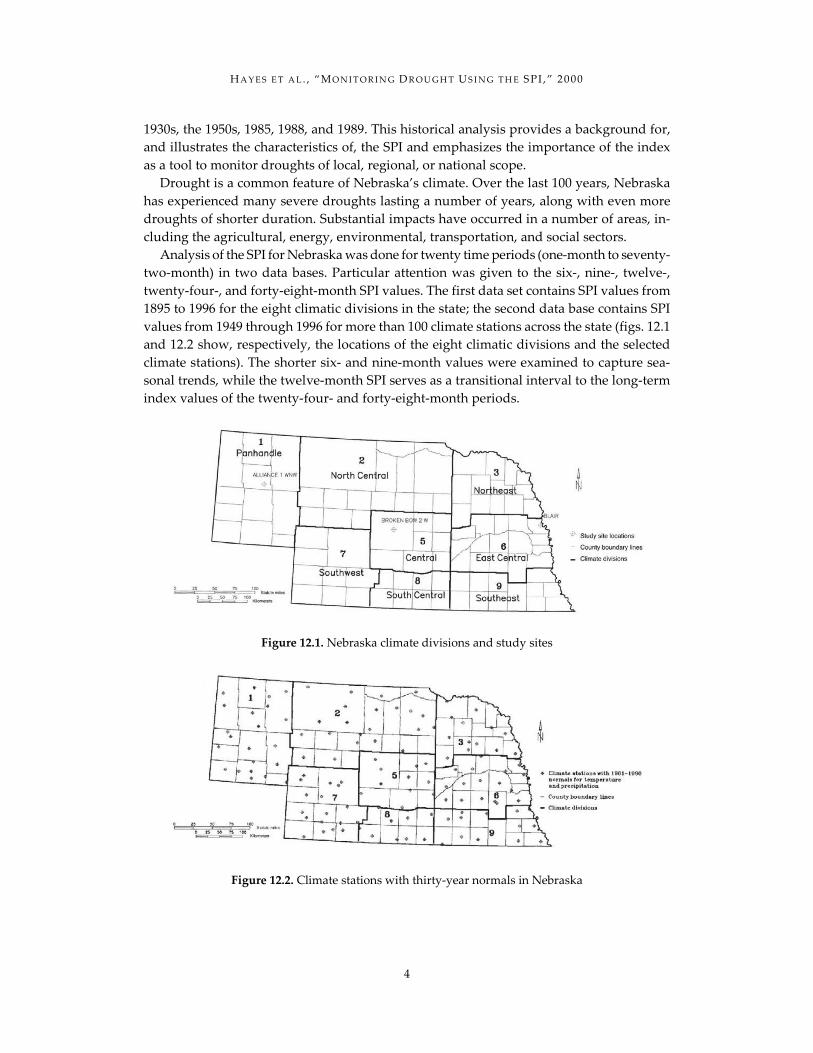
Analysis of the SPI for Nebraska was done for twenty time periods (one-month to seventy-two-month) in two data bases. Particular attention was given to the six-, nine-, twelve-, twenty-four-, and forty-eight-month SPI values. The first data set contains SPI values from 1895 to 1996 for the eight climatic divisions in the state; the second data base contains SPI values from 1949 through 1996 for more than 100 climate stations across the state (figs. 12.1 and 12.2 show, respectively, the locations of the eight climatic divisions and the selected climate stations). The shorter six- and nine-month values were examined to capture sea-sonal trends, while the twelve-month SPI serves as a transitional interval to the long-term index values of the twenty-four- and forty-eight-month periods.

Figure 12.1. Nebraska climate divisions and study sites

Figure 12.2. Climate stations with thirty-year normals in Nebraska


5

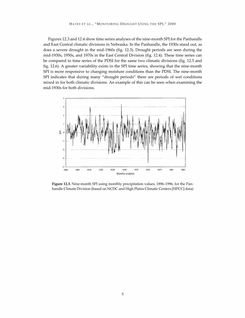
Figures 12.3 and 12.4 show time series analyses of the nine-month SPI for the Panhandle and East Central climatic divisions in Nebraska. In the Panhandle, the 1930s stand out, as does a severe drought in the mid-1960s (fig. 12.3). Drought periods are seen during the mid-1930s, 1950s, and 1970s in the East Central Division (fig. 12.4). These time series can be compared to time series of the PDSI for the same two climatic divisions (fig. 12.5 and fig. 12.6). A greater variability exists in the SPI time series, showing that the nine-month SPI is more responsive to changing moisture conditions than the PDSI. The nine-month SPI indicates that during many “drought periods” there are periods of wet conditions mixed in for both climatic divisions. An example of this can be seen when examining the mid-1930s for both divisions.

Figure 12.3. Nine-month SPI using monthly precipitation values, 1896–1996, for the Pan-handle Climate Division (based on NCDC and High Plains Climatic Centers [HPCC] data)


6

Figure 12.4. Nine-month SPI using monthly precipitation values, 1896–1996, for the East Central Climate Division (sources as for fig. 12.3)

Figure 12.5. Palmer Drought Severity Index (PDSI) using monthly values. 1896–1996, for the Panhandle Climate Division (based on data from the Climate Prediction Center)


7

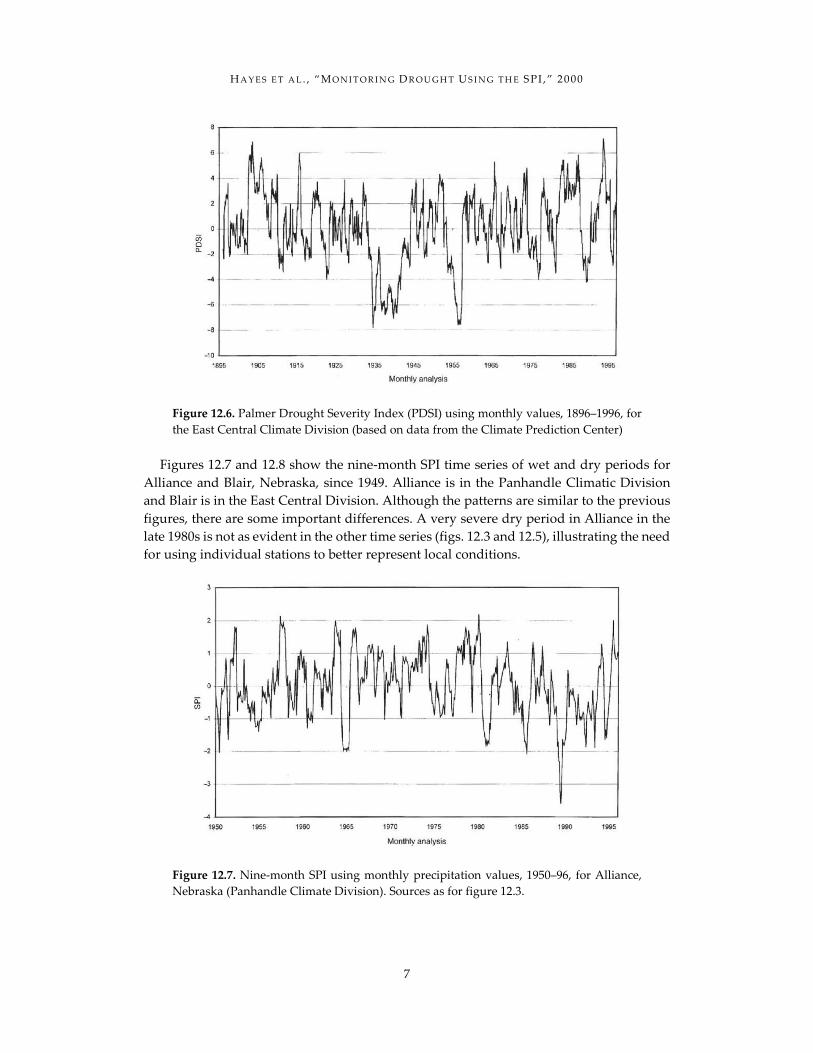
Figure 12.6. Palmer Drought Severity Index (PDSI) using monthly values, 1896–1996, for the East Central Climate Division (based on data from the Climate Prediction Center)

Figures 12.7 and 12.8 show the nine-month SPI time series of wet and dry periods for

Alliance and Blair, Nebraska, since 1949. Alliance is in the Panhandle Climatic Division and Blair is in the East Central Division. Although the patterns are similar to the previous figures, there are some important differences. A very severe dry period in Alliance in the late 1980s is not as evident in the other time series (figs. 12.3 and 12.5), illustrating the need for using individual stations to better represent local conditions.

Figure 12.7. Nine-month SPI using monthly precipitation values, 1950–96, for Alliance, Nebraska (Panhandle Climate Division). Sources as for figure 12.3.


8

Figure 12.8. Nine-month SPI using monthly precipitation values, 1950–96, for Blair, Ne-braska (East Central Climate Division). Sources as for figure 12.3.

Figure 12.9 is an example of using site data to interpolate SPI values across the state.

The two-year period ending in December 1989 indicates that conditions were very dry in both the western and eastern parts of the state. Much of the eastern quarter of the state was in severe drought as defined by the SPI. The drought of 1988–89 was very severe and had a substantial impact on the entire Corn Belt region. The eastern half of Nebraska makes up the western edge of the Corn Belt. By using the site values, the variability that frequently occurs within each climatic division (fig. 12.1) can be seen.

Figure 12.9. Twenty-four-month SPI through the end of December 1989 Sources: McKee et al. 1993, NDMC 1997, High Plains Climate Center 1997

In the case of Alliance and the Panhandle Division, a small pocket of severe drought is

seen in the twenty-four-month SPI values in the immediate area, but most of the Panhandle


9

is experiencing only moderate drought or near-normal conditions. This provides a better picture for local conditions rather than relying on a single representative value for the en-tire climatic division, and it explains why the SPI time series for Alliance is so low (fig. 12.7) while the climatic division time series is not (fig. 12.3). The use of local SPI infor-mation has been very useful for determining the impacts of weather on crop yields (Ya-moah et al. 1997).

Tables 12.2–12.4 summarize drought occurrences from 1949 to 1996 for Alliance, Broken Bow, and Blair, Nebraska (for locations of these towns, see fig. 12.1). Broken Bow is located in the Central Climatic Division. McKee et al. (1993) define a “drought event” as the period when the SPI is continuously negative and reaches an intensity of –1.0 or less. The drought would then end when a positive value occurs. These three sites were chosen to provide a cross-section of drought occurrences across the state. For some of the SPI time periods, two droughts are shown to illustrate that the longest droughts are not necessarily the most intense and might not have the largest impacts or damages associated with them. Factors such as the time of onset or the mean intensity instead of the duration should be looked at in addition to the magnitude and peak intensity. For example, the longest drought period at Alliance using the twelve-month SPI lasted 37 months, from 1990 to 1993 (table 12.2). However, the drought of 1987–90, with a peak intensity of –4.28 (extreme drought) and a mean intensity of –1.27, had a greater impact on the area.

For Broken Bow (table 12.3), three drought periods during the 1949–1996 period were identified. The drought of longest duration, eighty-one months, began in 1966 and con-cluded in 1973. However, the drought of 1952–58, lasting sixty-seven months, had a peak intensity of –3.53 (extreme drought) and a mean intensity for the duration of the drought that fell into the severe classification at –1.60. The analysis for Blair, Nebraska, is shown in table 12.4.

Table 12.2. 1949–96 SPI drought analysis for Alliance, Nebraska

Years SPI interval

(months) Duration (months)

Peak intensity

Mean intensity

1990–93 12 37 –1.67 –0.89 1987–90 12 33 –4.28 –1.27 1988–95 24 83 –2.98 –1.23 1983–96 48 153 –3 –1.06

Table 12.3. 1949–96 SPI drought analysis for Broken Bow, Nebraska

Years SPI interval


Peak intensity

Mean intensity

1952–57 12 58 –2.62 –1.4 1952–57 24 61 –2.88 –1.61 1952–58 48 67 –3.53 –1.63 1966–73 48 81 –1.25 –0.65


10

Table 12.4. 1949–96 SPI drought analysis for Blair, Nebraska

Years SPI interval


Peak intensity

Mean intensity

1974–77 12 37 –1.94 –1.15 1953–59 24 69 –2.39 –1.13 1954–60 48 68 –2.67 –1.2 1976–82 48 74 –1.76 –0.89

After the Dust Bowl years of the 1930s, the 1950s are generally considered the next worst

years in terms of prolonged drought within Nebraska in the modern era. At the drought’s peak in the middle of the decade, nearly two-thirds of the state was experiencing severe or extreme drought. Even at the twenty-four-month time period (fig. 12.10), severe drought is evident in all but the Panhandle region in the state. Of course, drought severity levels fluctuated, but a severe or extreme classification (SPI values <–1. 5) over a two-year period is a strong signal of persistent drought. Figure 12.10 gives a quick picture of the potential impacts expected given the general lack of irrigation at the time. Shorter-term SPI values (six-, nine-, and twelve-month analysis) during the same time frame (mid-1950s) illustrate the ebb and flow of extreme drought values (SPI <–2.0) and spatial extent across the state.

Figure 12.10. Twenty-four-month SPI through the end of December 1956. Sources as for figure 12.9.

The tendency of fewer but longer droughts was found in the 24- and 48-month SPI av-

eraging periods (table 12.5). In the years since 1949, Alliance has experienced ten 12-month SPI drought periods, six 24-month drought periods, and two 48-month drought periods. This trend held true across the other climatic divisions as well. Broken Bow had twelve 12-month, six 24-month, and three 48-month droughts while Blair showed eleven 12-month, seven 24-month, and three 48-month SPI drought periods.


11

Table 12.5. Drought frequency across Nebraska, 1949–96 Location SPI time period Number of droughts

Alliance 12 10 24 6 48 2 Broken Bow 12 12 24 6 48 3 Blair 12 11 24 7 48 3

Table 12.6 shows the variation in precipitation both across the state and within the cli-

matic divisions. This table demonstrates why there is a need to use climatic division data with caution, depending on the scale of monitoring efforts. In some years, the divisional data does a good job of representing some of the individual sites; in other years, the depar-ture from the division average can be extreme. This is especially true in the Great Plains region, where convective precipitation is “hit and miss” for any given location during the spring and summer months.

Table 12.6. Annual rainfall by site and climatic division Location 1934 1953 1965 1989 1993

Panhandle 10.98 17.12 21.67 11.92 21.8 Alliance 8.78 13.89 21.73 9.57 17.52 East Central 15.85 21.38 39.98 22.26 39.71 Lincoln 17.23 17.55 45.15 23.82 39.21

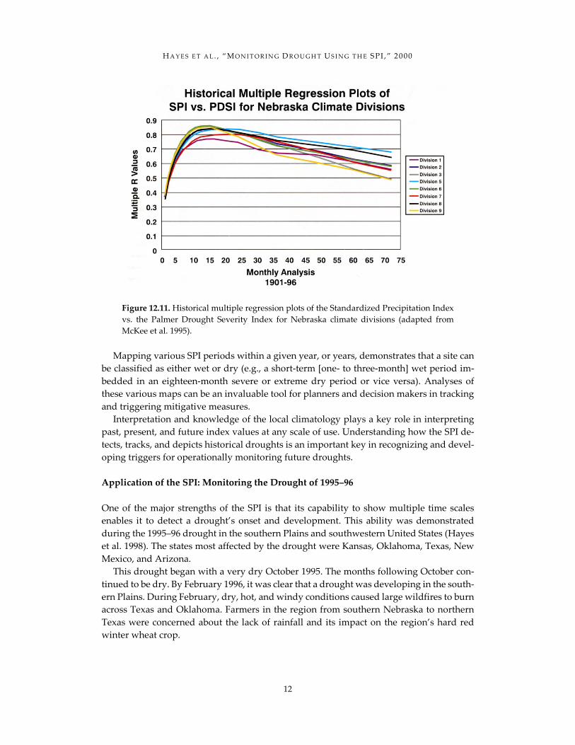
In comparing the SPI to the PDSI for the Panhandle (Climatic Division 1) and East Cen-

tral (Climatic Division 6) climatic divisions in Nebraska, initial findings of the relationship for monthly values (1895–1996) are very similar to those that McKee et al. (1993, 1995) found for Fort Collins, Colorado (fig. 12.11). Looking at the twelve-month period, the cor-relation coefficient for the Panhandle was 0.76 while the twenty-four-month value dropped only slightly, to 0.75. For the East Central Division, the twelve-month correlation was also the strongest, with a value of 0.86. The twenty-four-month value was 0.81. For both divisions, the values were much lower for the nine- and six-month relationships. Thus, the inherent time scale of the PDSI shows a larger lag in response time to current conditions than does the SPI, which can be computed from one to twelve months. As seen in figure 12.11, the strongest relationship between the PDSI and SPI for all of the climatic divisions was generally found in the twelve- to fifteen-month range, where r2 values were greater than 0.80.


12

Figure 12.11. Historical multiple regression plots of the Standardized Precipitation Index vs. the Palmer Drought Severity Index for Nebraska climate divisions (adapted from McKee et al. 1995).

Mapping various SPI periods within a given year, or years, demonstrates that a site can

be classified as either wet or dry (e.g., a short-term [one- to three-month] wet period im-bedded in an eighteen-month severe or extreme dry period or vice versa). Analyses of these various maps can be an invaluable tool for planners and decision makers in tracking and triggering mitigative measures.

Interpretation and knowledge of the local climatology plays a key role in interpreting past, present, and future index values at any scale of use. Understanding how the SPI de-tects, tracks, and depicts historical droughts is an important key in recognizing and devel-oping triggers for operationally monitoring future droughts. Application of the SPI: Monitoring the Drought of 1995–96 One of the major strengths of the SPI is that its capability to show multiple time scales enables it to detect a drought’s onset and development. This ability was demonstrated during the 1995–96 drought in the southern Plains and southwestern United States (Hayes et al. 1998). The states most affected by the drought were Kansas, Oklahoma, Texas, New Mexico, and Arizona.

This drought began with a very dry October 1995. The months following October con-tinued to be dry. By February 1996, it was clear that a drought was developing in the south-ern Plains. During February, dry, hot, and windy conditions caused large wildfires to burn across Texas and Oklahoma. Farmers in the region from southern Nebraska to northern Texas were concerned about the lack of rainfall and its impact on the region’s hard red winter wheat crop.


13

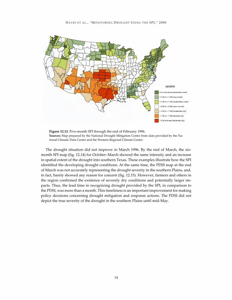
By the end of February, a chart prepared by the Joint Agricultural Weather Facility (fig. 12.12) depicted precipitation for the October 1995–February 1996 period in this winter wheat region as the second lowest over the past 101 years. The five-month SPI map for the country (fig. 12.13) was also clearly showing the dryness for the October–February period in the southern Plains. Most of the climatic divisions from southern Nebraska to northern Texas, which includes the winter wheat region, were at least in the “severely dry” category (SPI values ≤–1.5). Dry conditions also appeared in the Southwest from southern California to New Mexico.

Figure 12.12. Precipitation departure from normal in the hard red winter wheat region for the five-month period October–February for 1896–1996 Sources: Data supplied by NCDC; map prepared by Joint Agricultural Weather Facility.


14

Figure 12.13. Five-month SPI through the end of February 1996. Sources: Map prepared by the National Drought Mitigation Center from data provided by the Na-tional Climatic Data Center and the Western Regional Climate Center.

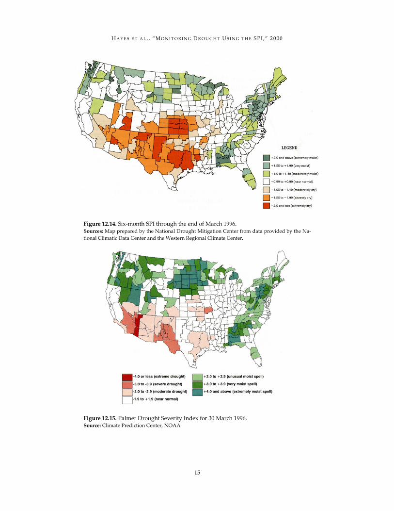
The drought situation did not improve in March 1996. By the end of March, the six-

month SPI map (fig. 12.14) for October–March showed the same intensity and an increase in spatial extent of the drought into southern Texas. These examples illustrate how the SPI identified the developing drought conditions. At the same time, the PDSI map at the end of March was not accurately representing the drought severity in the southern Plains, and, in fact, barely showed any reason for concern (fig. 12.15). However, farmers and others in the region confirmed the existence of severely dry conditions and potentially larger im-pacts. Thus, the lead time in recognizing drought provided by the SPI, in comparison to the PDSI, was more than a month. This timeliness is an important improvement for making policy decisions concerning drought mitigation and response actions. The PDSI did not depict the true severity of the drought in the southern Plains until mid-May.


15

Figure 12.14. Six-month SPI through the end of March 1996. Sources: Map prepared by the National Drought Mitigation Center from data provided by the Na-tional Climatic Data Center and the Western Regional Climate Center.

Figure 12.15. Palmer Drought Severity Index for 30 March 1996. Source: Climate Prediction Center, NOAA


16

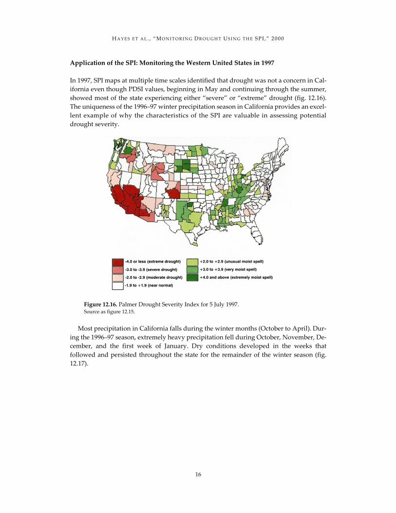
Application of the SPI: Monitoring the Western United States in 1997 In 1997, SPI maps at multiple time scales identified that drought was not a concern in Cal-ifornia even though PDSI values, beginning in May and continuing through the summer, showed most of the state experiencing either “severe” or “extreme” drought (fig. 12.16). The uniqueness of the 1996–97 winter precipitation season in California provides an excel-lent example of why the characteristics of the SPI are valuable in assessing potential drought severity.

Figure 12.16. Palmer Drought Severity Index for 5 July 1997. Source as figure 12.15.

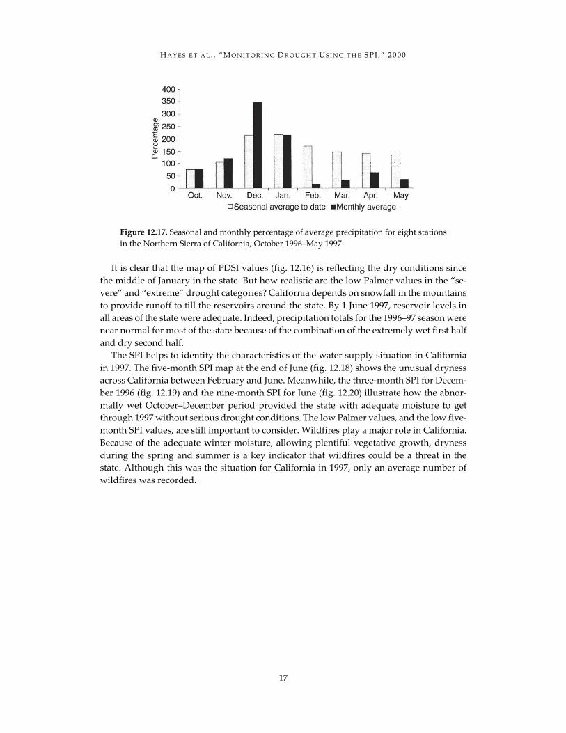
Most precipitation in California falls during the winter months (October to April). Dur-

ing the 1996–97 season, extremely heavy precipitation fell during October, November, De-cember, and the first week of January. Dry conditions developed in the weeks that followed and persisted throughout the state for the remainder of the winter season (fig. 12.17).


17

Figure 12.17. Seasonal and monthly percentage of average precipitation for eight stations in the Northern Sierra of California, October 1996–May 1997

It is clear that the map of PDSI values (fig. 12.16) is reflecting the dry conditions since

the middle of January in the state. But how realistic are the low Palmer values in the “se-vere” and “extreme” drought categories? California depends on snowfall in the mountains to provide runoff to till the reservoirs around the state. By 1 June 1997, reservoir levels in all areas of the state were adequate. Indeed, precipitation totals for the 1996–97 season were near normal for most of the state because of the combination of the extremely wet first half and dry second half.

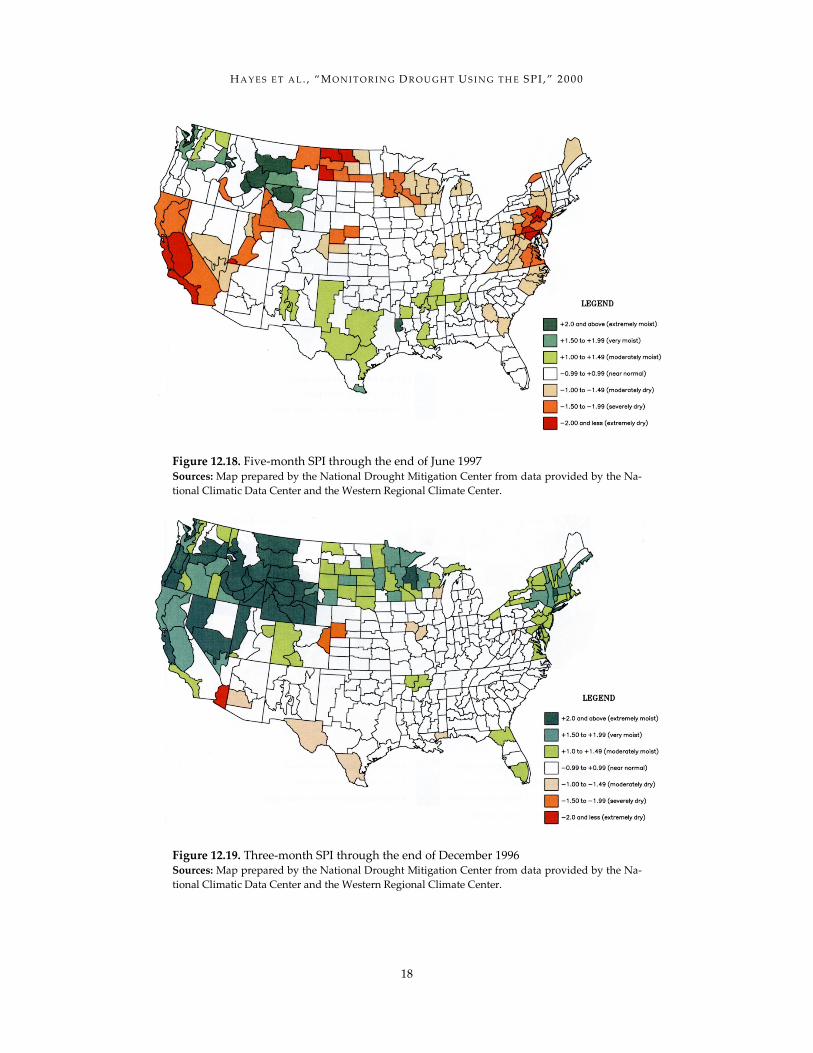
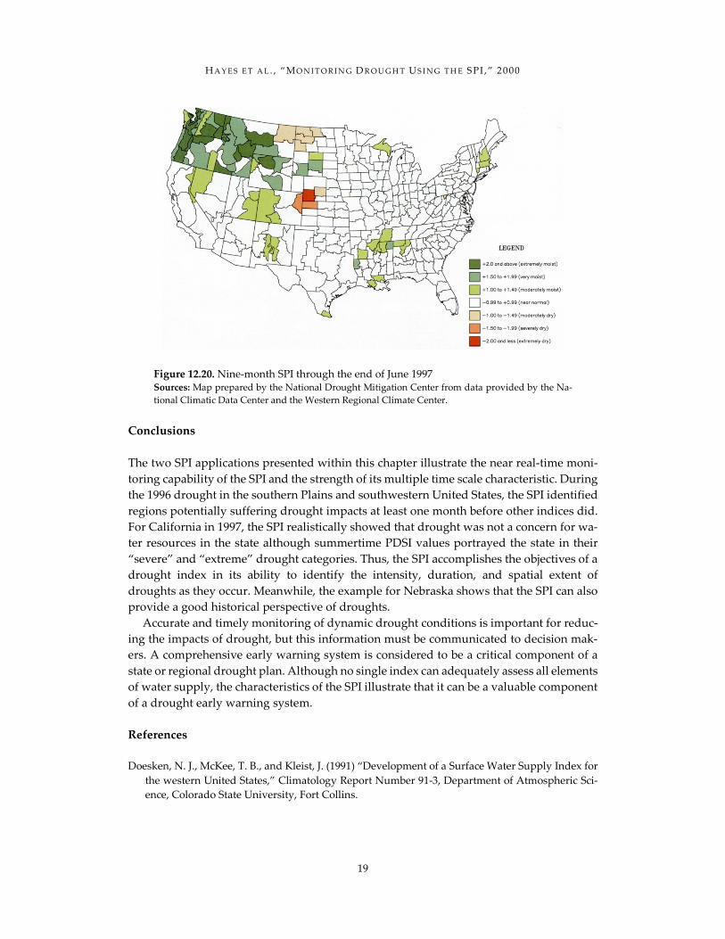
The SPI helps to identify the characteristics of the water supply situation in California in 1997. The five-month SPI map at the end of June (fig. 12.18) shows the unusual dryness across California between February and June. Meanwhile, the three-month SPI for Decem-ber 1996 (fig. 12.19) and the nine-month SPI for June (fig. 12.20) illustrate how the abnor-mally wet October–December period provided the state with adequate moisture to get through 1997 without serious drought conditions. The low Palmer values, and the low five-month SPI values, are still important to consider. Wildfires play a major role in California. Because of the adequate winter moisture, allowing plentiful vegetative growth, dryness during the spring and summer is a key indicator that wildfires could be a threat in the state. Although this was the situation for California in 1997, only an average number of wildfires was recorded.


18

Figure 12.18. Five-month SPI through the end of June 1997 Sources: Map prepared by the National Drought Mitigation Center from data provided by the Na-tional Climatic Data Center and the Western Regional Climate Center.

Figure 12.19. Three-month SPI through the end of December 1996 Sources: Map prepared by the National Drought Mitigation Center from data provided by the Na-tional Climatic Data Center and the Western Regional Climate Center.


19

Figure 12.20. Nine-month SPI through the end of June 1997 Sources: Map prepared by the National Drought Mitigation Center from data provided by the Na-tional Climatic Data Center and the Western Regional Climate Center.

Conclusions The two SPI applications presented within this chapter illustrate the near real-time moni-toring capability of the SPI and the strength of its multiple time scale characteristic. During the 1996 drought in the southern Plains and southwestern United States, the SPI identified regions potentially suffering drought impacts at least one month before other indices did. For California in 1997, the SPI realistically showed that drought was not a concern for wa-ter resources in the state although summertime PDSI values portrayed the state in their “severe” and “extreme” drought categories. Thus, the SPI accomplishes the objectives of a drought index in its ability to identify the intensity, duration, and spatial extent of droughts as they occur. Meanwhile, the example for Nebraska shows that the SPI can also provide a good historical perspective of droughts.

Accurate and timely monitoring of dynamic drought conditions is important for reduc-ing the impacts of drought, but this information must be communicated to decision mak-ers. A comprehensive early warning system is considered to be a critical component of a state or regional drought plan. Although no single index can adequately assess all elements of water supply, the characteristics of the SPI illustrate that it can be a valuable component of a drought early warning system. References Doesken, N. J., McKee, T. B., and Kleist, J. (1991) “Development of a Surface Water Supply Index for

the western United States,” Climatology Report Number 91-3, Department of Atmospheric Sci-ence, Colorado State University, Fort Collins.


20

Edwards, D. C., and McKee, T. B. (1997) “Characteristics of 20th century drought in the United States at multiple time scales,” Climatology Report Number 97-2, Department of Atmospheric Science, Colorado State University, Fort Collins.

Hayes, M. J., Svoboda, M. D., Wilhite, D. A., and Vanyarkho, O. V. (1999) “Monitoring the 1996 drought using the Standardized Precipitation Index,” Bulletin of the American Meteorological Soci-ety 80, 3: 429–38.

McKee, T. B., Doesken, N. J., and Kleist, J. (1993) “The relationship of drought frequency and dura-tion to time scales,” Proceedings of the Eighth Conference on Applied Climatology, Boston, MA: Amer-ican Meteorological Society.

McKee, T. B., Doesken, N. J., and Kleist, J. (1995) “Drought monitoring with multiple time scales,” Proceedings of the Ninth Conference on Applied Climatology, Boston, MA: American Meteorological Society.

Yamoah, C., Hayes, M. J., and Svoboda, M. D. (1997) “Application of the Standardized Precipitation Index to estimate crop yields in Nebraska,” Proceedings of the Tenth Conference on Applied Clima-tology, Boston, MA: American Meteorological Society.

chapter 12 monitoring drought using the standardized

Documents