- Bogotá - Colombia - Bogotá - Colombia - Bogotá - Colombia - Bogotá - Colombia - Bogotá - Colombia - Bogotá - Colombia - Bogotá - Colombia - Bogotá - Colombia - B

The Effects of In utero Programs on Birth Outcomes:

The Case of “Buen Comienzo” *

Lina Cardona-Sosa† Carlos Medina‡

Banco de la República de Colombia

Abstract

This paper studies the effects of an in utero program on birth outcomes addressed to vulnerable

pregnant women. We use information from the Buen Comienzo program, an initiative run by the

local government of Medellin, the second largest city of Colombia. In order to identify the

effects we obtain matching estimates using data from program participants and the census of

birth statistics. We find that the program increased the birth weight of participant children by

0.09 and 0.23 standard deviations for boys and girls, respectively, and reduced the prevalence

of low birth weight by 2.6 and 4.6 ppts for boys and girls, respectively. In terms of size, the

program reduces the incidence of being short by 3 and 4 ppts, for boys and girls, respectively.

The program also significantly reduced preterm births between 3 and 8 ppts. We also provide

evidence of the existence of heterogeneous effects depending on a mother’s exposure to the

program and her frequency of attendance. Finally, an estimate of the cost-benefit ratio of the

program suggests that its benefits could be 2 to 6 times its costs, respectively for boys and girls

born from participant mothers with early exposure to the program.

JEL Classification codes: I38, J13, J18 Keywords: Early childhood programs, program evaluation, selection on observables.

* The authors thank the administrators of the Buen Comienzo Program and their technical team for their help with the data. We are very grateful to Juan Felipe Gonzalez, Henry Puerta, and Gladys Restrepo for all their support understanding the program. This document has also benefited from comments by participants in different seminars: NIP-Network of Inequality and Poverty, 2013; I-Early Childhood Seminar in EAFIT-Medellín, 2014; Universidad Javeriana Seminar, 2014, and internal seminar at the Banco de la República (Central Bank of Colombia), and two anonymous referees. The series Borradores de Economía is published by the Economic Studies Department at the Banco de la República. The works published are provisional, and their authors are fully responsible for the opinions expressed in them, as well as for possible mistakes. The contents of the works published do not compromise Banco de la República or its Board of Directors. † Researcher. Corresponding author. Calle 50 No. 50-21, Banco de la República, Medellín. E-mail address: lcardoso@banrep.gov.co ‡ Manager Medellín Branch. E-mail address: cmedindu@banrep.gov.co

El Efecto de Programas dirigidos a Madres Gestantes en Indicadores al Nacer:

El caso de “Buen Comienzo” *

Lina Cardona-Sosa†

Carlos Medina‡

Banco de la República de Colombia

Resumen

Este documento examina los efectos de una estrategia dirigida a madres gestantes en

condiciones de vulnerabilidad sobre los indicadores de sus hijos al nacer. Para lo anterior se

usa información administrativa del programa Buen Comienzo, una iniciativa lanzada por el

gobierno local de Medellín, la segunda ciudad más grande de Colombia. Con el fin de

identificar el efecto, se obtienen estimadores de emparejamiento o matching usando datos de

madres participantes del programa así como del censo de estadísticas vitales. Se encuentra que

el programa aumentó el peso al nacer de hijos de madres participantes en 0.09 y 0.23

desviaciones estándar para niños y niñas respectivamente, reduciendo la incidencia de bajo

peso al nacer en 2.6 y 4.6 pp respectivamente. En cuanto a la talla al nacer, el programa Buen

Comienzo habría reducido la probabilidad de tener baja talla en 3 y 4 pp para niños y niñas en

cada caso. En términos de nacimientos prematuros, los resultados muestran una reducción en

su probabilidad de entre 3 y 8 pp. Finalmente, se encuentra evidencia de efectos diferenciales

del programa dependiendo del tiempo de exposición y frecuencia de asistencia a la estrategia.

En términos de costo-beneficio nuestros estimados sugieren que los beneficios del programa

podrían estar entre 2 y 6 veces sus costos en el caso de niños y niñas nacidos de madres

participantes con exposición temprana al programa.

Clasificación JEL: I38, J13, J18 Palabras clave: peso al nacer, atención a la primera infancia, evaluación de programas, selección basada en observables, matching.

* Los autores agradecen a los administradores del programa Buen Comienzo y a su equipo técnico por su ayuda con los datos. En particular el apoyo de Henry Puerta, Juan Felipe Gonzalez y Gladys Puerta por todo su apoyo entendiendo el programa. Este documento se ha beneficiado de los comentarios de los participantes a diferentes seminarios: NIP Network of Inequality and Poverty, 2013; I-Seminario de Primera Infancia en EAFIT-Medellín, 2014; Seminario Universidad Javeriana, 2014, seminario interno del Banco de la República, y dos referees anónimos. La serie Borradores de Economía es una publicación de la Subgerencia de Estudios Económicos del Banco de la República. Los trabajos son de carácter provisional, las opiniones y posibles errores son responsabilidad exclusiva de los autores y sus contenidos no comprometen al Banco de la República ni a su Junta Directiva. † Investigadora. Autora corresponsal. Calle 50 No. 50-21, Banco de la República, Medellín. Correo electrónico: lcardoso@banrep.gov.co ‡ Gerente Banco de la República Sucursal Medellín. Correo electrónico: cmedindu@banrep.gov.co

1. Introduction

Birth outcomes have been found to be important predictors of a child’s health in the short run

as well as of different outcomes as an adult in the long run. While in the short run birth

outcomes are related to child mortality (Barker, 1989), in the long run, they affect an adult’s

education and health (Barker, 2006), and, as a result, the individual’s labor market

performance, one of the determinants of poverty and inequality.

Previous studies have found that a 10% increase in birth weight represents a one-year

reduction of children’s mortality and a 1% increase in future earnings (Black, 2007). Similarly, a

0.57 cm increase in a child’s size is translated into a 0.06 higher IQ score at age 18 (in a scale

from 1 to 9). The importance of previous indicators relies on the support that economists and

governments have provided to policy strategies aiming to improve nutrition, education and

health for children under five. Following Heckman (2010), a child’s inputs exhibit higher

malleability at this stage with higher long-term returns in cognitive and non-cognitive skills

(Heckman et al. 2010; Cunha et al. 2006). Thus, birth weight is an important factor that early

childhood programs should consider due to its role in improving skills that affect poverty

transmission. In this paper, we examine one of the early-childhood strategies launched in

Colombia and its effects on children’s birth outcomes (weight and size), with the purpose of

identifying not only the effectiveness of the program, but also its potential, long-run

contribution.

In Colombia, infants weighing under 2,500 grams (or with Low Birth Weight, LBW) account

for 8.7% of all newborns regardless of their gestational length (Pinzón-Rondón, et al. 2015).

To place the previous figures in context, the lower incidence of LBW can be found in

developed countries (3%), while the highest can be found in South Asia (40%). Furthermore,

the incidence of LBW in Colombia gains importance considering that of all infants born

worldwide, 15.5% have low birth weight, and among them 96% are located in developing

countries.

Nevertheless, the incidence of LBW is not homogeneous across Colombian population. By

gender, the proportion of girls born with LBW is 9%, while among boys the proportion is 7%.

By health insurance, the incidence of LBW among those attending the subsidized regime (low

income households and vulnerable population) is between 7.9% and 8.3%. In Colombian rural

areas, the incidence of LBW is even higher. The percentage of infants born with LBW is 7.3%

and 7.9% for boys and girls, respectively. Moreover, big cities such as Bogotá and Medellín are

experiencing some of the highest incidence of LBW in the country (13% and 9.1%,

respectively, in 2010).

Governments around the world have implemented different strategies addressed to

disadvantaged households with the aim of affecting early childhood development. In the US,

programs such as The Perry School Meal Program, the Milwakes Project, and the Abecedarian

Project have been addressed to improve nutrition and education among children. In Bolivia

and Colombia, PIDI and Hogares Comunitarios, respectively, have attempted to improve

children’s development, and they have made some evidence available.

In contrast to the programs addressing the needs of young children, the ones aimed at

pregnant women (or in utero programs) have been less explored by the literature. Programs with

such characteristics include the Women, Infant and Children (WIC) in the US, and the

Uruguayan program PANES (or Plan de Atencion Nacional a la Emergencia Social). Nevertheless,

additional anti-poverty strategies also affect a mother’s health during pregnancy. This is the

case of the Food Stamp Transfer Program (FSP) in the US, or the conditional cash-transfer

programs in Latin America such as Bolsa Scuola in Brazil, Progresa/Oportunidades in Mexico, and

Familias en Acción in Colombia.

The main advantage of the programs addressed exclusively to pregnant women is that they do

not only provide in-kind transfers, but also interdisciplinary support during pregnancy and

training to future parents, which has been found to be effective in early childhood programs

(Bernal et al., 2010). However, little is yet known about the effect of in utero programs in

Colombia, which is the aim of this study.

In 2009, the Colombian municipality of Medellín launched the in utero component of the

program Buen Comienzo, an early childhood strategy addressed to affect infants’ early

development. The strategy consists of two elements: providing the nutritional supplement for

pregnant women, and parental training. In this paper, we study the effects of the first

component, targeted at pregnant women. We examine short-run outcomes such as birth

weight, height, and the APGAR score (Appearance, Pulse, Grimace, and Respiration). Due to

the non-random assignment of the program, we follow a non-experimental setting to identify

the effects. To do so, we link administrative information from program beneficiaries to vital

statistics data from the compilation of births in the country. To complement the demographic

information of our data, we link this information with the one available in the means-test

classification system available in Colombia (SISBEN).

Our results suggest that Buen Comienzo increased the birth weight of girls from participant

mothers by a 0.23 standard deviation (SD), which is equivalent to a 115 gram increase in

weight, approximately. Moreover, among boys, the increase in weight was about 45 grams (i.e.,

0.09 SD). We state that this increase corresponds to an upper bound of the program’s effect

since this is observed for those attending the program once a month after the first trimester of

pregnancy. This provides evidence of the importance of not only being treated, but also of the

intensity of the program. Regarding children’s height, we found an increase of 0.19 standard

deviations among treated girls (or a 0.45 cm increase) for those attending the program.

Moreover, after simulating a cost/benefit relation, we found that the benefits of the program

are between 2 and 6 times its cost for boys and girls, respectively.

This paper is organized as follows. The next section discusses the causes of LBW and its

consequences. The third section describes the main features of the program Buen Comienzo,

while section four discusses the methodology used for the analysis. Section five describes the

data, and section six presents the results. Section seven discusses the main findings, and finally

section eight concludes.

2. Causes and Consequences of Low Birth Weight

Low birth weight (henceforth LBW) can result from two different factors: fetal growth

retardation (commonly known as intra-uterine growth retardation, IUGR) or a gestational

length below 37 weeks (pre-term birth). While the causes of prematurity are less well

understood and consequently are less explored in the literature (Kramer, 1987), most studies

have focused on the understanding of fetal growth retardation and its impacts on LBW.

The medical literature has identified the following factors as the main predictors of intra-

uterine growth retardation: poor nutrition during pregnancy, lower mother’s weight and

stature, mother’s economic activity, prenatal care, poor mother’s health, for example, suffering

from diabetes or malaria during pregnancy (see Kramer, 1987 for a complete survey of

literature’s main findings). In contrast, pre-term births have been found to be explained by

previous abortions and pre-term births, poor pre-pregnancy weight, and inadequate prenatal

care, mother’s physical and economic activities, stress and cigarette smoking, among others.

But, which factors should policy makers focus on? The answer depends on the main source of

a country’s LBW. Kramer’s study concludes that while most of the LBW incidence in

developed countries is due to pre-term births, intra-uterine growth retardation is the main

explanation for the incidence observed in the developing world. This should not be surprising

if we consider that nutrition, one of the factors delaying a fetus’ growth, is an issue in many

developing countries. As for Colombia, the latest government figure suggests that half of LBW

is due to IUGR, and the other half to preterm births (Quiroga, 2015).

Particularly in Colombia, previous studies have found that previous abortion experiences,

inadequate weight gain during pregnancy, diabetes, inadequate prenatal control, mother’s

stress, anxiety or depression, mother’s ingestion of alcohol, coffee or drugs, and some

environmental issues are the main risk factors for having LBW. Regarding mothers’ age, being

over 35 or being a teenage mother (younger than 20) also affects the probability of being born

below 2,500 grams. This figure gains relevance in a country like Colombia since the incidence

of LBW among teenage mothers is about 12% (above the national figure of 9%), and accounts

for 22% of total births in the country (Quiroga, 2015).

More recently, the study by Pinzón-Rondón, et al. (2015) shows that the absence and quality of

prenatal care and the number of visits to the doctor account for some of the most important

determinants of LBW in Colombia.

Following the previous studies, there is scope for policy makers to affect LBW by affecting

modifiable factors. In fact, when the source of LBW is IUGR, it is possible to affect a

mother’s nutrition or to provide antenatal care, whereas if the source for LBW is mainly

gestational length, a mother’s habits (alcohol consumption, stress, etc.) can be also affected via

parental training, in addition to an increase in the mother’s caloric intake. Moreover, the role of

public policy in reducing LBW becomes more relevant when more evidence about the long-

lasting effects of improving birth weight is found in the literature. As a matter of fact,

economists have provided plenty of evidence showing that LBW has significant medium and

long-lasting effects on education and employment. In the presence of IUGR, LBW affects an

individual’s academic performance through his/her deficit of micronutrients, which accounts

for the deficit in weight. For instance, iodine deficits directly affect children’s cognitive

development and mental retardation (Black, 2003), while lack of folic acid (folate) increases the

risk of a neural tube defect (Black et al. 2008). Both of them affect a child’s future academic

performance.

Furthermore, estimating the causal effect of LBW on an individual’s outcomes is challenging

because unobserved factors affecting a child’s birth weight such as genetics, parental interest,

and motivation, among others, could be correlated with the outcomes under study (health,

education, and employment). In order to overcome this, most studies have relied on within-

twin comparisons, a method whose advantage is to keep constant observable and

unobservable family and household characteristics. Hence, twins living in the same household,

sharing the same mother, and facing the same environment with the same gestational length

would differ mainly in their birth weight due to differences in vitamin intake before birth.

Something similar could be concluded from siblings’ studies, except for the fact that they lack

the same gestational length.

Behrman and Rosenzweig (2004) use the within-twins variation technique for a sample of

monozygotic (identical) twins in the US. The study finds that birth weight is an important

predictor of an adult’s height and that it affects negatively an adult’s labor market outcomes.

Following their results for the US, a 481 gram (17 oz) increase in birth weight among LBW

children would increase an individual’s life time earnings by 10%. Although the analysis is

conducted for a very restricted sample (only monozygotic twins), a similar conclusion

regarding labor market earnings was found in the siblings’ study by Johnson et al. (2011). In

fact, the authors find that LBW children see their labor market earnings reduced by 15%.

Also using within-twin variation (fraternal and monozygotic twins) and data from Norway,

Black et al. (2007) show that a 10% increase in a child’s birth weight reduces his/her mortality

probability by one-year. Similarly, they find that a 0.57 cm increase in size at birth increases an

individual’s IQ score by 0.06 at age 18 (in a scale from 1 to 9). The study also finds that high-

school completion rates increase in a proportion below 1 ppts, while earnings are augmented

by 1%. In terms of next-generation effects, they find that an improvement in today’s children’s

birth weight will lead to an increase in their offspring’s birth weight.

Another study exploiting within-twin variation is the one by Royer (2009), who estimates the

effect of LBW on long-run outcomes of Californian and British children. He finds that a 1 kg

increase in birth weight is related to a 0.13 increase in the number of years of education. Since

there is a negligible probability that a program reaches a 1,000 gram increase in birth weight,

the authors translate the previous effects into a lower scale, showing that a 200 gram increase

in weight increases the number of years of education by 0.03 for an average child, and by 0.08

for those born under 2,500 grams. In a different study for the US, adding siblings to the

analysis, Fletcher (2011) finds that a child with LBW has a 4 ppts higher probability of

repeating a grade in the school.

Glewwe et al. (2001), using siblings rather than twins’ data and longitudinal information for

Filipino children, find that a higher birth weight is related to a better school performance. In a

similar study using Scottish data, Lawlor et al. (2006) find that among all male siblings, a 1 SD

increase in birth weight is translated into higher IQ scores by age 7.

Although this finding was observed by keeping the mother’s gestational length constant, other

studies have found that being preterm (e.g., with a gestational length below week 37) also has

negative effects on children’s cognitive scores (see the meta-analysis written by Bhutta et al.

2002).

In terms of health outcomes, using twins’ data, Almond et al. (2005) find that a 1 SD increase

in child’s birth weight reduces infant mortality by 0.41 SD, improves the APGAR score by 0.5

SD, and reduces children’s assisted ventilation by 0.25 SD. The authors also provide an

estimation of hospital costs related to LBW. The study finds that a 1 SD increase in birth

weight or a 667 gram increase is equivalent to a USD 3,200 reduction in hospitalization costs.

In line with the previous finding, the study by Glewwe et al. (2001) estimates that per each

dollar invested in programs aiming to improve birth weight through nutritional strategies, three

dollars will be returned through its improvement on a child’s educational performance.

Although within-twins studies allow to identify the causal effect of LBW for a given gestational

length, there is some concern about twins’ representativeness of the general population

(usually twins occur in less than 1% of the population). Hence, among the other alternative

approaches explored by literature on LBW to identify its effects, exogenous changes such as

policy reforms, introduction of new programs or institutional shocks have been studied (see

Currie and MacLeod (2008); Hoynes et al. (2009); and Hoynes et al. (2012); Alderman (2007)

for some of them).

Alderman et al. (2007) combine both methods. The first method exploits within-siblings

variation, while the second one uses civil war shocks to identify differences on nutrition across

siblings. They find that a 3.4 cm taller child increases the number of grades completed at

school by 0.85 and reduces the entrance at school by 6 months. Similarly, Alderman et al.

(2001) use price shocks during the pre-school stage to see how early nutrition (measured with

height z-score) affects enrollment rates in rural Pakistan, finding a negative effect.

A previous study by Almond et al. (2010) explores a regression discontinuity design to identify

the effect of having a very low birth weight (1,500 grams) on hospital costs. The study shows

that an infant born above 1,500 grams sees his/her probability of one-year mortality reduced

by 1 ppt, while a child with birth weight below 1,500 grams increases hospital costs by 10%.

Other sets of studies have used instrumental variables to identify the effect of weight

indicators such as height versus age on long-run outcomes. For instance, Glewwe et al. (2005)

use distance to health facilities and father’s height as instruments to explain height versus age.

His findings support evidence that lower height versus age delays school entrance.

Very few studies using cross-sectional records have addressed the selectivity problem that

arises when identifying the effects on children’s outcomes on interventions directed to

vulnerable populations (See Bitler and Currie, 2005 who do examine this bias). Linear

regression approaches have been conducted for Estonia by Rahu et al. (2010), finding that a

500 gram increase in birth weight is associated with a 0.7 point increase in a child’s IQ scores.

The increase in the IQ score as a result of a higher birth weight was also observed for all

Danish men living in a particular region (Sorensen et al., 2007). Although administrative data

have many advantages and reduce some self-selectivity bias present in some surveys, they

suffer from some bias due to unobservable variables driving both, birth and adult outcomes.

2.1 In-kind programs affecting LBW

What types of strategies have worked in reducing the incidence of LBW? Previous

research has found that, in the presence of IUGR, intake of the following micro-nutrients has

reduced the incidence of LBW due to IUGR: folic acid, iodine, vitamin B6, protein, and iron

(Kramer, 1987). Thus, food supplement programs could have an important effect on a child’s

birth weight. Following Black (2005), who also uses within-twin techniques, treated moms see

their child’s birth weight increased by 7.5%. Bitler and Currie (2004) also find that, although

mothers attending the Women, Infants and Children program are a negative selected sample of

the population, there is a positive effect on children’s birth outcomes for eligible mothers.

They increase their probability of attending prenatal care since the first trimester by 6%, while

the probability of being born under the 25th percentile of child’s weight distribution is around

2% for a given gestational length. Moreover, the study finds that such an effect is even larger

among teenage mothers and high school dropouts.

More recently, Currie and Rajani (2014) use the mothers’ fixed effects and New York

administrative records to identify the effect of WIC on birth outcomes. The study finds that

treated infants see their probability of having LBW reduced by 5.6%, while the probability of

being small for their age is reduced by 4.9%. Moreover, for firstborns, the probability of being

born with LBW is reduced by a third. Foster et al. (2010) reached a similar finding by using a

propensity score matching approach according to which the program reduced the probability

of LBW by 1 percent.

Almond et al. (2008) exploit the timing of operation of the Food Stamp Program between

counties. The authors find a 7% reduction in the incidence of LBW among mothers exposed

to the program with infants at the bottom of the weight distribution. Figlio et al. (2009), using

large administrative data and implementing RDD, find that WIC participation reduced the

probability of having LBW and very high birth weights.

3. Description of the Program

Buen Comienzo is an early childhood strategy launched by the local government of

Medellín addressed to families with young children (below age 6) with the purpose of

promoting children’s healthy development, early stimulation, and nutrition and parental

training. Program strategies are delivered through different modalities depending on the child’s

age, as follows: pregnant and breastfeeding mothers and children up to 1 year old; children

from 1 to 2 years old; children from 2 to 4; and children from 5 to 6. From them, pregnant

mothers are the subcomponent that we studied.

The program trains future parents during pregnancy, with support from an interdisciplinary

group of professionals including nutritionists, social workers, psychologists, pedagogues, and

physical educators. Parents are invited to attend the program when they visit the doctor for

first time during pregnancy. By becoming beneficiaries of Buen Comienzo, they are offered a

nutritional supplement once a month and three hours of parental training every two weeks.

Less regularly, they receive visits from different professionals to complement their training at

home. The nutritional supplement accounts for 20% of a mother’s daily nutritional

requirement, and it includes the following micro-nutrients: calcium, folic acid, zinc, iron and

vitamin B.

Figure 1. Number of sessions attended by treated mothers during their pregnancy

Source: Author’s own calculations based on the administrative records from the program

Although attendance to the program is not mandatory, mothers are self-encouraged to attend

at least once a month, which is usually the session when the nutritional supplement is

0

2

4

6

8

10

12

14

16

1 2 3 4 5 6 7 8 9 10 11 12 13 14 15 16 17 18 19 20 21 22 23 24

Perc

en

t

delivered1. Nevertheless, the program’s professionals work very hard at motivating parents to

attend twice a month, explaining to them the importance of the training. Figure 1 shows the

number of sessions attended by participant mothers per month. In fact, it shows that the

largest frequency is that of participant women attending only once and an important fraction

of them attended less than 7 sessions (which could be once per month after they know they

are pregnant). Mothers are weighted every session, and a special follow-up is made to those

mothers with low pregnancy weight. Unfortunately, the administrative information of the

program for the period analyzed did not keep a complete record of this.

3.1 Program eligibility

In order to be eligible for the gestational component of the program, pregnant women

were required to register in the proxy-means testing Colombian system, SISBEN 2. This

system is based on an index that weights households’ demographic characteristics (e.g.,

income, education, wealth, etc.) collected around 2005, assigning a score between 0 and 100

to each household. The system classifies households into six different levels according to this

score, where level 1 accounts for the most disadvantaged households and level six

corresponds to the less disadvantaged ones. In general, applicants eligible to government

programs are those households in levels 1 and 2 of SISBEN 2 (see Bottia et al., 2012), which

was the case for pregnant women applying to Buen Comienzo. The system was updated in 2009

to become SISBEN 3 (which is the year when the gestational strategy of Buen Comienzo was

introduced) changing the way the SISBEN score was estimated and defining a new threshold

for household eligibility into the program. In the interim, administrators of Buen Comienzo

simultaneously accepted households who held the conditions under the old classification (i.e.,

those belonging to levels 1 and 2 of SISBEN 2) and households already re-classified in the

new version with equivalent conditions (i.e., those scoring less than 47.99 in SISBEN 3).

Moreover, most of households had already been re-classified under the new version so their

eligibility conditions were based on having a SISBEN 3 score below 47.99. Displaced

households, victims of the conflict, and those belonging to ethnic minorities were

automatically eligible for the program, as were those mothers whose pregnancy was at risk

such as teenagers (around 22% of all mothers) and women above 35 years of age (8% of all

mothers).

Although the SISBEN score requirement was meant to be a necessary condition (as well as

sufficient for whoever applied) for program eligibility, in practice there were beneficiaries and

non-beneficiaries on both sides of the SISBEN 2 and 3 cutoffs. Pregnant mothers who were

potentially eligible for the program were invited to be part of it during their first visit to the

doctor. The program took place in public health facilities of the city; hence, at the beginning,

the physicians and health practitioners from public health centers were the ones who

promoted participation in the program. In some cases, the strategy came to be known by the

mothers through neighbors or friends. Furthermore, mothers who were considered at risk due

to their age, low gestational weight, or any sickness were particularly encouraged to be part of

the program. Similarly, mothers already receiving government support due to their poverty

conditions would also be invited and highly encouraged to participate in the program.

Although there is no official record of the take up rate of the program or how many mothers

attended the program from all those who received the invitation, anecdotal evidence suggests

that the nutritional supplement and the free biscuits were an important motivation for mothers

to attend the sessions at least once.

Figure 2. Mothers who attended Buen Comienzo during pregnancy and breastfeeding period.

2009-2014

Source: Data taken from Medellín’s education indicators 2004-2014 (Secretary of Education) based on Program

attention data for 2009-2010 and the Buen Comienzo Information System 2011-2014.

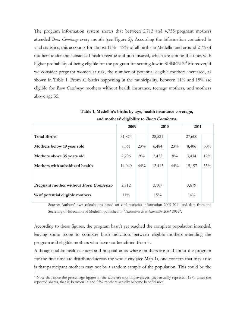
The program information system shows that between 2,712 and 4,755 pregnant mothers

attended Buen Comienzo every month (see Figure 2). According the information contained in

vital statistics, this accounts for almost 11% - 18% of all births in Medellín and around 21% of

mothers under the subsidized health regime and non-insured, which are among the ones with

higher probability of being eligible for the program for scoring low in SISBEN 2.4 Moreover, if

we consider pregnant women at risk, the number of potential eligible mothers increased, as

shown in Table 1. From all births happening in the municipality, between 11% and 15% are

eligible for Buen Comienzo: mothers without health insurance, teenage mothers, and mothers

above age 35.

Table 1. Medellin’s births by age, health insurance coverage,

and mothers’ eligibility to Buen Comienzo.

2009 2010 2011

Total Births 31,874 28,521 27,600

Mothers below 19 year sold 7,361 23% 6,484 23% 8,406 30%

Mothers above 35 years old 2,796 9% 2,422 8% 3,434 12%

Mothers with subsidized health 14,040 44% 12,413 44% 15,197 55%

Pregnant mother without Buen Comienzo 2,712 3,107 3,679

% of potential eligible mothers 11% 15% 14%

Source: Authors’ own calculations based on vital statistics information 2009-2011 and data from the

Secretary of Education of Medellín published in "Indicadores de la Educación 2004-2014".

According to these figures, the program hasn’t yet reached the complete population intended,

leaving some scope to compare birth indicators between eligible mothers attending the

program and eligible mothers who have not benefitted from it.

Although public health centers and hospital units where mothers are told about the program

for the first time are distributed across the whole city (see Map 1), one concern that may arise

is that participant mothers may not be a random sample of the population. This could be the

4 Note that since the percentage figures in the table are monthly averages, they actually represent 12/9 times the reported shares, that is, between 14 and 25% mothers actually become beneficiaries.

case if mothers living in slightly better neighborhoods become more motivated to be part of

the program, or if, on the contrary, those in worse conditions are persuaded to attend. In both

cases, the effect of the program could be biased by unobserved factors (physicians, mother’s

motivation, etc.) which may affect participation in the program and birth outcomes. Map 1a

shows the distribution of beneficiaries across the city, and Map 1b shows the average

socioeconomic stratum of the area in which the neighborhood is located. The socioeconomic

stratum is the way in which the population is classified based on residential location with the

purpose of targeting subsidies to the country’s residential public utilities services, with

households living in stratum 1 being the poorest and those living in stratum 6 the wealthiest.

Map 1b to the right shows that most of the disadvantaged neighborhoods are located mainly in

the north of the city, where most of the beneficiaries live. Moreover, there is still a high

percentage of births in deprived areas (strata 2 and 3) which were not covered by the program

at the beginning, leaving some scope to compare birth outcomes among similar mothers

participating and not participating into the program.

Map 1. Distribution of beneficiaries of Buen Comienzo

a. b.

Source: Authors’ own calculations based on Vital statistics information 2009-2011 and data from the Secretary of

Education of Medellín published in “Indicadores de la Educación 2004-2014”.

4. Empirical Strategy

As previously stated, once pregnant women are identified at public health centers, they

are invited to enroll Buen Comienzo, provided they meet the eligibility requirements that made

them vulnerable. Nonetheless, and as shown above, not all potential eligible mothers have

been cared for by the strategy, allowing us to compare participant and non-participant mothers

from all eligible mothers. As previously stated, one of the eligibility conditions required by the

program is having a SISBEN 3 score below 47.99; however, the high number of exceptions

made by program administrators (e.g., being displaced, being younger than 20 or older than 35,

as well as experiencing other risk factors) did not allow for the SISBEN score to work as the

actual forcing variable. In fact, when testing for the existence of a discontinuity in the

probability of being treated with the SISBEN cutoff, we found no significant evidence of it

(see figure A.1 in the Appendix), which led us to discard the possibility of using a regression

discontinuity approach to identify the effects of the intervention, at least for the phase of the

program considered (2009-2011). Therefore, we followed a matching approach based on the

assumption that pregnant women self-select into the program based on their observable

characteristics. There are several variables that might affect both women’s selection into the

program and the assessed outcomes, which we were not able to observe, which include

ethnicity, parent’s height and weight, mother’s cigarette and alcohol consumption, etc.

(Kramer, 1987). Our estimates would still be unbiased once we condition on our set of

observables, as long as these unobserved variables were balanced. Since we were able to

control for a wide set of characteristics, we expect this to have been the case. Particularly, we

expect newborns with equally aged and educated parents, similar household sizes, income,

socioeconomic stratum, home ownership, health insurance type of coverage, etc.; to be similar

in their unobservable traits regardless of whether or not they were beneficiaries of the program

(Bitler and Currie, 2005).

The conceptual framework is based on the child’s health production function (Yi), which is

determined by the genetic endowment, captured, in part, through a child's family

characteristics. Other inputs affecting a child's health nutrition and parental care provided, (li),

among other components which affect the newborn’s health (ui).

𝑌𝑖 = 𝑓(𝐹𝑖; 𝐼𝑖; 𝑢𝑖) (1)

The reduced form would be given by

𝑌𝑖 = 𝛽0 + 𝛽1𝐹𝐴𝑀𝐼𝑖 + 𝛽2𝑋𝑖 + 𝛽3𝐼𝑖 + 𝜀𝑖 (2)

Where Yi is a proxy for a child's i nutrition at birth (e.g., weight and size). FAMi corresponds

to the child’s set of socio-demographic background (e.g., parent’s age and schooling, parent’s

economic activity, income, etc.). Similarly, Xi corresponds to the vector of individual

characteristics of the child at birth, such as mother’s duration of the pregnancy, child’s gender,

type of birth, among others. Ii is an indicator for additional inputs that the child receives. This

includes a nutritional complement and better parental care. Finally, 𝜀𝑖 corresponds to other

factors that affect the health status of the newborn.

The estimation of the effect of the program Buen Comienzo on birth outcomes can be framed

into the model for potential outcomes proposed by Roy-Rubin (Roy [1951]; Rubin [1978])

which defines participation in the program as the treatment under study and participating

individuals as the treated individuals.

The model starts with the existence of a binary treatment (participation and non-participation)

where the indicator for treatment, Di, is defined as equal to 1 if the individual i is treated, and

as 0 otherwise. There are two potential outcomes (Yi(Di)) for the same individual: the outcome

under treatment Yi(1) and without treatment (Yi(0)). Hence, the effect of the treatment (Ti) for

individual i could be written as the difference in outcomes between the participating and non-

participating individual:

Ti = Yi(1) - Yi(0) (3)

Nevertheless, the main problem with any program evaluation (equation 3) is that it is not

possible to observe the same individual under both states, i.e., as an individual participating in

the program in the state of non-participation. In other words, the main difficulty is that we

cannot observe Yi(0), therefore, we face a missing data problem (Caliendo [2006];Blundell and

Dias [2009]). An alternative way to estimate (3) would be to average the participants’ outcome

and subtract it from the one for non-participants. Nevertheless, by doing so, we would add

bias to the estimate given that participants and non-participants could differ systematically in

their characteristics even in the absence of the program. Similarly, participants may not be a

random sample of the population, and could have particular characteristics that defined their

participation into the program, which at the same time could be affecting some of the

individuals’ outcomes under study.

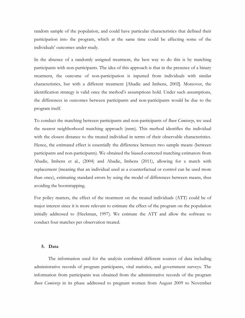
In the absence of a randomly assigned treatment, the best way to do this is by matching

participants with non-participants. The idea of this approach is that in the presence of a binary

treatment, the outcome of non-participation is inputted from individuals with similar

characteristics, but with a different treatment [Abadie and Imbens, 2002]. Moreover, the

identification strategy is valid once the method’s assumptions hold. Under such assumptions,

the differences in outcomes between participants and non-participants would be due to the

program itself.

To conduct the matching between participants and non-participants of Buen Comienzo, we used

the nearest neighborhood matching approach (nnm). This method identifies the individual

with the closest distance to the treated individual in terms of their observable characteristics.

Hence, the estimated effect is essentially the difference between two sample means (between

participants and non-participants). We obtained the biased-corrected matching estimators from

Abadie, Imbens et al., (2004) and Abadie, Imbens (2011), allowing for a match with

replacement (meaning that an individual used as a counterfactual or control can be used more

than once), estimating standard errors by using the model of differences between means, thus

avoiding the bootstrapping.

For policy matters, the effect of the treatment on the treated individuals (ATT) could be of

major interest since it is more relevant to estimate the effect of the program on the population

initially addressed to (Heckman, 1997). We estimate the ATT and allow the software to

conduct four matches per observation treated.

5. Data

The information used for the analysis combined different sources of data including

administrative records of program participants, vital statistics, and government surveys. The

information from participants was obtained from the administrative records of the program

Buen Comienzo in its phase addressed to pregnant women from August 2009 to November

2011. Among the information available, there is the national identification number for each

participating mother, date of entry into the program, the phase of the participant (pregnant or

lactating), among others. Although the information is presented as an unbalanced panel of

participants (with a monthly frequency), we use it as a cross-section relying on the fact that

each participant could attend several sessions during the period analyzed.

The information on birth weight, height, and health outcomes was obtained from the vital

statistics dataset, a census of all individuals born alive in a particular year. We matched the

mothers’ information from this source and the dataset mentioned above to identify the birth

outcomes of treated women. One concern is that the births registered in the vital statistics

dataset are underreported (Duryea et al., 2006). Following the study by Duryea et al., (2006)

this was the case in urban areas, mainly due to the lack of parental identification, lack of time,

or proper stationary at the place of register. Moreover, the study reports a national average of

16% of unreported births in the country, a rate that is lower in Medellín, the city where the

program took place (4%). Similarly, in the case of the sample used for the analysis (to match

treated and untreated mothers), all of them are registered in SISBEN, which implies the need

to have parental identification, a condition that reduces the probability of not having registered

the births.

To create the counterfactual (i.e., the group of non-participants), we merged vital statistics

information with data from SISBEN, a system that allocates a score to households according

to their socioeconomic characteristics (amenities, income, etc.) and classifies them into six

levels, where level 1 identifies the most disadvantaged and level 6 refers to the least

disadvantaged individuals. As mentioned previously, the government used this classification to

allocate education and health subsidies to households classified in the first three levels of

SISBEN.

The SISBEN dataset for Medellin has information on approximately 1,500,000 individuals (out

of a total population of 2,500,000, excluding the metropolitan area). This corresponds to 60%

of the city’s population, all of them in socio-economic disadvantages. To identify which

mothers did not participate in the program, the dataset of participants was merged with the

data from SISBEN (already merged with vital statistics), defining the SISBEN group that was

not merged with participants' information to conform the untreated or control group.

Merging the three datasets leaves us with 41,659 observations for mothers (including their

children's outcomes), which is the sample that we will use for the estimations. The treated

group has 19,525 observations, and the control group (mothers not attending the program)

reaches 22,134 observations. Depending on the outcomes analyzed, the observations will be

slightly reduced.

5.1 Birth Outcomes

The main outcomes studied here are birth weight, size at birth, and APGAR (Appearance,

Pulse, Grimace and Respiration). Following the literature, we started by estimating the

standardized version (or z-score) for weight and height, respectively (i.e., each outcome is

normalized to have mean 0 and a standard deviation of 1). The APGAR is built as a dummy

variable which takes the value of 1 if the child scores between seven and ten, which are the

normal measures for vital signs at birth during the first and 5th minute after birth.

Additional indicators for birth weight and size are also examined following the World Health

Organization (WHO) standards, which have been adopted by the Colombian law to

characterize children’s growth and their nutritional state per Resolution 2121 of 2010. We use

weight per age, which in our case corresponds to a child's birth weight. We define each of the

child’s weight outcomes according to the position of a child's weight with respect to the mean

and standard deviation proposed by the WHO at a particular age, by gender. This is how

several indicators used to define a child’s weight can be analyzed (see Table 2). This is the case

for very low weight, low weight, at risk of low weight, and normal weight. Similarly, the

indicators for children's height are: low height, at risk of low height, and normal height.

Other additional indicators that can be used include those based on weight versus size, which

is the recommended measure to define overweight and obese children, opposite to the Body

Mass Index (BMI), which is the common indicator used to measure those outcomes for

children over 2 years of age. Hence, we include children across all the birth weight distribution,

differentiating them by using weight categories (very low birth weight, low birth weight,

normal weight, overweight, etc.)

Table 2 shows the criteria used to define the different categories each child belongs to

according to his/her birth outcomes. Similarly, Table 3 reports the different cut-offs at which

every child would be categorized into one of the groups mentioned above. We built dummy

variables indicating whether or not each child's outcomes belong to that classification.

Table 2. Reference measures for children in Colombia

< -3 sd

< -2 sd

< -1 sd

0 > 1 sd > 2 sd

> 3 sd

Boys' weight (kg) 2.1 2.5 2.9 3.3 3.9 4.4 5.0

Girls' weight (kg) 2.0 2.4 2.8 3.2 3.7 4.2 4.8

Boys' height (cm) 44.2 46.1 48.0 49.9 51.8 53.7 55.6

Girls' height (cm) 43.6 45.4 47.3 49.1 51.0 52.9 54.7

Boys' BMI (kg/m2) 10.2 11.1 12.2 13.4 14.8 16.3 17.7

Girls' BMI (kg/m2) 10.1 11.1 12.2 13.3 14.6 15.1 18.1

Source: Colombian Resolution 00002121 of 2010.

Table 3. Criteria to classify children’s birth indicators according to his/her anthropometric measures

A. WEIGHT Very low weight < -3 SD

Low weight < -2 SD

At risk of low weight > - 2 SD, < - 1 SD

Appropriate weight > - 1 SD, < 1 SD

B. HEIGHT Low height < -2 SD

At risk of low height > - 2 SD, < - 1 SD

Appropriate height > - 1 SD

C. BMI Overweight > 1 SD, < 2 SD

Obese > 2 SD

Source: Colombian Resolution 00002121 of 2010.

5.2 Descriptive Statistics

The matched sample between SISBEN and vital statistics data accounts for 46.726 mothers.

From them, we excluded those mothers for whom we were unable to determine the number of

months they had attended the program, or those with unlikely answers. Thus we ended up

with a sample of 40,229 mothers. Among them, 14,865 were treated and 25,364 were included

in the control group. Moreover, following previous literature (Behrman et al., 2004), there

could be heterogeneous effects from a particular treatment depending on an individual’s

differences regarding exposure to the program and their frequency of attendance. Thus, we

built three different treatment groups accounting for that difference. Treatment 1 corresponds

to the whole sample of treated mothers participating in the program regardless of their time of

exposure and frequency of attendance; treatment 2 includes only treated individuals who

entered the program from the first quarter of their pregnancy period; treatment 3 comprises

treated mothers who entered during their third quarter of pregnancy. It is important to take

into account that this group (treatment 3) includes mothers who, according to officials of the

program, is heavily represented by mothers who have been diagnosed at risk due to difficulties

during their pregnancy such as anemia or low gestational weight.

Finally, treatment 4 corresponds to those mothers who not only entered the program during

the first quarter of their pregnancy, but also attended at least once a month in the last 6

months of their gestational length. In all cases, the control group was the same: mothers who

were not participating in the program Buen Comienzo. We ended up with four different samples,

whose sizes varied according to the group under analysis. Group 1 (which included treatment 1

and its respective control group) accounted for 40,229 mothers; group 2 (accounting for

treatment 2 and the usual control group), included 29,146 mothers; group 3, 29,146, and group

4 included 27,635 mothers.

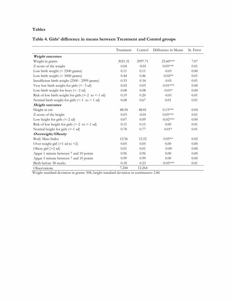
The main set of variables characterizing the sample and each group are presented in Tables 4

to 7. Tables 4 and 5 report, for boys and girls, respectively, the difference in the main

outcomes between treated and control mothers in our most extended definition of treatment

(i.e., regardless the time of exposure into the program). Tables 6 and 7 compare the main set

of demographic variables between treated and control mothers, separately by gender of the

newborn. These variables were included in the matching procedure. The set of variables

included from SISBEN and vital statistics data includes: mother’s characteristics (e.g., marital

status, years and levels of education, economic activity, strata, housing, and health insurance);

level of education and age of a child’s father; and a child’s birth characteristics such as type of

labor (or delivery type), whether or not there was a multiple birth, whether or not the SISBEN

score was below 47.99, timing after the birth was registered, and birth year dummies.

The comparison reported in the previous tables allows inferring that children from participant

mothers have better birth outcomes than those from the control group (higher birth weight

and height). Moreover, the comparison between demographic characteristics shows that

participant mothers are slightly more disadvantaged individuals than non-participants. In fact,

participant mothers have less years of education, and are more likely to have completed

primary education versus secondary education. Similarly, they are less likely to be working and

are more likely to belong to strata 1. Thus, following Currie et al., (2004), in the presence of

negative selection of the treated population, the existence of a positive effect would imply the

existence of the impact.

6. Estimates of the Program’s Impact on Birth Outcomes

Tables 8 and 9 show the birth weight estimates from the nearest neighborhood

matching approach for girls and boys, respectively. Each row corresponds to a different

anthropometric category used as dependent variable. With the exception of the z-score, all

outcomes are expressed as indicator variables, i.e., showing the change in a child’s probability

of being in each of the weight categories. Every table shows the estimated outcome for each of

the treatment groups in four different columns. The estimates from Column (1) of each table

refer to the first group considered in the analysis (the one using treatment 1). In this case, the

estimates would indicate whether or not there is an effect of the program among all participant

mothers regardless of the date they started attending the program or their frequency.

Following the estimates from Column (1) in Table 8, the results suggest that the program

improves girls’ birth weight by a 0.06 standard deviation (e.g., 30 grams). Similarly, the

program reduces the probability of a girl experiencing low birth weight and a very low birth

weight by 1 ppt in each case.

In the next set of columns we test for the existence of heterogeneous effects as suggested by

Behrman et al., (2004), we examine whether or not mothers attending the program with

different exposure and frequency experienced a different effect. Column (2) estimates the

impact of Buen Comienzo restricting the treated group to those mothers attending the program

from the first quarter of their pregnancy. With a smaller sample, results suggest a 0.19 SD

improvement on girls’ birth weight, and a significant reduction on the probability of being

born with LBW. There is a reduction in the probability of having low birth weight by 3.7 ppts

and of having very low birth weight by 3.1 ppts. Similarly, the probability of being born with

normal weight increases by 5 ppts.

The estimates for birth size using the second treatment group also suggest that the program

increased girls’ size at birth by 0.15 standard deviations (i.e., 37 mm), and reduced the

probability of being born short (i.e., below 45 cm) by 4 ppts. Once we restricted our treatment

group for mothers attending the program since the last quarter of their gestational period

(Column (3)), the estimates showed fewer evidences of the program’s effect on birth

outcomes. In relation to this group 3 (which is over represented by mothers at risk), it is

important to point out that our set of covariates does not include information of the mother’s

health status either at the baseline or during their pregnancy, therefore, we are unable to

control for such traits if present among mothers. We must bear this limitation in mind at the

moment of interpreting the results obtained for mothers included in this group 3, whose

prevalence of such traits is known to be much more frequent. This will very likely prevent us

from being able to obtain an appropriate match of them from mothers in the control group,

potentially leading us to obtain underestimated effects of the program.

Frequency of attendance is another factor that affects the outcome of an intervention

(Behrman et al., 2004). In Column (4), we examine whether this was the case during the first

stage of the program Buen Comienzo. For those estimates, the sample was restricted to mothers

who attended the program since their first quarter of pregnancy, attending the program’s

sessions at least once a month in the last six months of their gestational period. The estimates

suggest that the program increased girls’ birth weight by 0.23 SD (which is around a 115 gram

increase in girls’ birth weight), and reduced the incidence of having LBW (following the

reference for girls suggested in Tables 2 and 3) by 4.6 ppts, and the probability of being born

below 2,500 grams by 5.4 ppts5. The reduction of LBW incidence is above the one found in

Uruguay (1.9 – 2.4 ppts) for the cash-transfer program PANES (Amarante et al., 2015),

suggesting that in-kind transfer programs might have a higher impact on children’s health.

The results in this column also suggest that the program reduced the probability of having very

low birth weight by 3 ppts, and the risk of being born with LBW by 2.4 ppts.

5 LBW and having a birth weight below 2.500gr are included as different outcomes. We did this because in the

case of girls, LBW defined as a BW 2SD below the average population, correspond to having a weight below 2.400gr. In the case of boys both indicators are the same.

In terms of birth size, Column (4), in the lower panel of the same Table, shows a reduction in

the probability of being short and being born shorter than 45 cm by 4.6 ppts6, while the

coefficient for the z-score of size at birth increased by 0.19 SD.

Table 9 presents the program’s impacts among boys born from participant mothers. As

previously stated, each set of Columns accounts for each of the treatment groups considered in

the analysis. The estimates from Column (2) suggest that mothers attending the program from

the first quarter of their pregnancy experienced a lower probability of having a boy with very

low birth weight or with LBW. In both cases the probability was reduced by 2 ppts. Similarly,

they were 3.6 ppts more likely to have a normal weight and 2.7 ppts less likely to be short. The

impact of the treatment for mothers who entered the program from the last quarter of their

pregnancy is null or negative (Column (3)). As in the case of girls, this result needs to be read

with caution since our set of covariates does not include information of the mother’s health

status either at the baseline or during their pregnancy, which is key to characterize the type of

mothers entering at this stage of the program as previously mentioned.

On the contrary, once we account for mothers with the highest exposure and a moderate

frequency of attendance (Column (4)), the results suggest that the program increased boys’

birth weight by 0.09 SD (or 45 grams, approximately), reduced the probability of LBW and

very low birth weight in 2.6 and 2.7 ppts, respectively, while it increased the probability of

experiencing normal weight by 3.6 ppts. Finally, the APGAR estimates (not shown in the

table) were found to be negligible7.

Another possible outcome that could be affected by the program is the probability of having a

pre-term birth, or being born before week 38. In fact, parental training, and good practices

such as the intake of vitamins and micro-nutrients are some of the factors that affect a

mother’s gestational length. Table 10 reports the results using as dependent variable an

indicator for whether or not mothers experienced a pre-term birth. Similar to the previous

tables, Table 10 presents the results in four sets of columns for each of the treatment groups

used in the analysis. Results suggest that treated mothers were less likely to have a pre-term

6 Low height and being shorter than 45cm are included as different outcomes. This was because in the case of

boys, having low height is defined as being shorter than 46cm. In the case of girls, both indicators are the same (i.e., below 45cm) 7 Results available upon request.

delivery. In fact, the probability was reduced between 3 and 9 ppts depending on a mother’s

exposure and frequency of attendance, i.e., a relative increase between 12.5% and 32% with

respect to the control’s mean. Boys and girls born from mothers attending the program are, on

average, 3.6 ppts less likely to be born pre-term (somewhat smaller to the effect found by

Haeck and Lefebvre, 2016, although statistically significant in this case). Similarly, boys whose

mothers attended the program since their first quarter of pregnancy experienced a reduction of

6.5 ppts in the probability, which is higher (7 ppts) once we account for those attending the

program at least once a month. As for girls born from treated mothers, the probability for

those attending the program since the first quarter and attending once a month, the probability

is reduced between 6.5 and 8.7 ppts, respectively (similar to the effect found by Bitler and

Currie, 2005).8

6.1 Balancing test for covariates

Table 11 reports the covariate balance for treated and control mothers for the matched sample.

By comparing the difference in means between the treatment and control groups that were

matched9 with its average difference, it is possible to see that the differences in the matched

sample are smaller than the ones presented in Tables 6 and 7. This provides evidence that the

matching procedure considerably reduced the difference between treated and control mothers

in terms of observable characteristics.

7. Cost-benefit analysis estimates

In this section, we propose a cost-benefit analysis of the program. To do so, we define the

following as “program benefits”: the positive evidence found on birth outcomes; the long-term

consequences of birth improvement (e.g., an individual’s productivity); and the consequential

reduction of bad outcomes (e.g., infant mortality, hospitalization, medical attention, etc.). The

cost of the program is the per capita amount of money allocated yearly by the municipality to

each participating mother. The unitary costs of each of the health practices and/or health

indicators (child’s mortality, hospitalization costs, etc.) were difficult to find and to estimate for

8 Both Haeck and Lefebvre (2016), and Bitler and Currie (2005), assess food and nutrition advice programs. 9 We conducted a covariate balance test for the extended group used in the analysis: treatment 1, which includes all mothers attending the program regardless of their time of exposure and number of days attended.

the Colombian case, mainly due to the lack of public information and available sources. Thus,

under the respective assumptions, we follow Behrman, Alderman and Hoddinott (2004) to

obtain benefit/cost ratios of the program. In this study, the authors provide health costs

estimates for average low/middle income country using information from different countries

in Africa, Asia and Latin America where birth weight and child’s indicators are usually a

concern.

The cost-benefit analysis is reported in Table 12. We will focus on the results for treatment

groups 2 and 4, given the potential limitations our methodology might have to identify the

effect of the program for mothers included in treatment group 3, as previously mentioned.

Nevertheless, the cost benefit analysis is presented for all groups.

The table includes our estimates for the program’s benefits and costs for each of the

populations considered in this study. We include benefits for children moving from below to

above the 2,500 kg threshold, and from increasing their height at birth. As Behrman, Alderman

and Hoddinott (2004) do, we provide an estimation of seven items that represent the benefits

of children leaving the status of being born with LBW. First, we include the benefits of

reducing infant mortality, estimated by the authors as a 7.8% reduction in the likelihood of a

child dying due to LBW, multiplied by the likelihood of the child moving out of LBW thanks

to the program. Then, we include the reduction in neonatal medical attention, estimated in

USD $255 per child born weighing less than 2,500 kg. By assuming that children born at the

hospital are about 90% of all, we assume that the costs for children born at home are 10% of

those for children who were born at the hospital. After multiplying the figure obtained by the

likelihood of the child moving out of LBW thanks to the program, the net present value of this

benefit for boys in the treatment 2 group is USD $4.9.

The third benefit is the reduced costs of subsequent illnesses and medical care for infants and

children, which is estimated to be around USD $48 per child born weighing less than 2,500 kg.

The net present value of this benefit for boys in the second group (column 3) is USD $1.0.

The fourth benefit considered in this analysis is the reduction of an individual’s lifetime

productivity due to stunting, which is estimated to be 2.2% of earnings. We estimate a child’s

future earnings in USD $2,500, then we discount this flow during 60 years, and multiply the

figure by the likelihood of the child moving out of LBW thanks to the program, obtaining a

net present value of USD $22.

The fifth benefit is the increase on an individual’s lifetime productivity thanks to the ability

increase when moving out of the LBW population, which is estimated to be 5.3% of lifetime

earnings, according to Behrman et al., (2004). After following a similar procedure to that of the

previous benefit, we obtain a net present value of this benefit of USD $53.

The last benefit we consider due to reductions in the share of children below 2,500 kg. is the

reduction of costs regarding chronic diseases, which is estimated to be 10 years of an

individual’s earnings, for a net present value of USD $2. For girls, we additionally consider an

intergenerational cost of being born with low weight. We follow Behrman, Alderman and

Hoddinott (2004), who estimate its potential effects by assuming that the children of LBW

mothers are born with a higher probability of having LBW, thus implying future costs which

must be discounted to its present value10. The estimated cost for girls in treatment group 2

(Column 4) is USD $52.4.

We then estimate the benefits of the program thanks to its effect on children’s health at birth.

As before, we use the estimates suggested by Behrman, Alderman and Hoddinott (2004): a 2%

increase in a lifetime’s earnings per a 0.25 standard deviation increase in children’s height. We

multiply the estimated earnings from the impact of the program by the children’s height,

measured by its impact on the z-score for height. For girls in treatment group 2 (Column 4),

the estimated benefits are USD $603. Thus, the total benefits are the sum of those obtained by

both birth weight and height.

The costs of the program are estimated to be USD $22 per month. By adopting a conservative

approach and assuming that treatment groups 1, 2, and 4, remain 7.5 months in the program

while treatment group 3 only remains 3 months, we calculate the total cost for each of the

treated mothers. The benefit/cost ratio calculated from the previous figures is reported in the

last row of the Table. It shows that when a participant mother is exposed to the program for

10 The assumptions of the authors are: (a) these effects are only for LBW mothers, not fathers;(b) on average,

they have four children, born when she is 17, 20, 26 and 35; (c) the probability for each of her children of being LBW given her mother was, is 20 percent; (d) this probability is 10 percent if the mother was not LBW; and (e) the benefits of reducing LBW for the children over their life cycles are the same as the benefits for the mothers, but lagged in time, with such possibilities over three generations of children.

7.5 months and attends at least six sessions, the benefits from the program are between 2 and

6 times as large as the costs for boys and girls, respectively. When eligible mothers who are

pregnant with girls are enrolled into the program since the first quarter of pregnancy the

benefit is 5 times the program’s costs. Columns (2) and (4) which are our preferred

specification reinforce the importance of exposure and frequency of attendance.

8. Conclusions

Using a matching estimator approach, we estimated the impact of a program run by the

local authorities of Medellín, the second largest city in Colombia. The program, named Buen

Comienzo (meaning “having a good start”), was addressed in one of its modalities to pregnant

women, promoting parental training and complementing mothers’ nutrition as its main

strategies. We assess its impact on children’s birth outcomes, estimating it separately for boys

and girls and in each case for four different treatment groups, according to the duration of

their exposure to the program and their frequency of attendance.

We found that the program impacts the birth weight of treated mothers positively on three-

out-of-four different treatment groups considered in the analysis: all participant mothers; those

enrolled in the program during the first quarter of pregnancy; and those enrolled in the first

quarter of pregnancy and attending once per month during the last six months of their

pregnancy. For the latter, the program reduced the likelihood of girls from treated mothers

being born underweight (i.e., below 2,500 kg) between 3 and 5 ppts. This result is slightly

above the reduction of the effects of LBW found among Uruguayan children from mothers

benefitted from cash-transfers programs (Amarante et al., 2015), suggesting the importance of

in-kind transfer programs.

The program also reduced the likelihood of boys being born below 2.5 kg by 2.6 ppts.

Similarly, the program also reduced the probability of being short (below 2 SD) by 5 and 4

ppts for girls and boys, respectively.

We also found that the program reduced the likelihood of children being born before week 38

in the same three treatment groups in magnitudes between 3 ppts for the whole sample

considered to around 9 ppts for the sample of treated women with the largest exposure to the

program.

After considering the total costs and benefits of the program for this population using some

estimates calculated for low/middle income countries (Behrman, Alderman and Hoddinott,

2004), we found that the benefit/cost relationship 2 for boys and 6 for girls. The program’s

benefits are also larger than its costs for the population of mothers who enrolled in their first

quarter of pregnancy and for those attending frequently the program. The results of the

evaluation pointed out the importance of mothers enrolling at an early stage of their pregnancy

in order to guarantee significant impacts on their children’s weight and height at birth.

Similarly, they state the lower benefit from the program that can be obtained when enrolling

late. Thus, detecting and enrolling pregnant mothers early in their pregnancy, preventing

mothers from enrolling late in their pregnancy, and making additional efforts to retain mothers

who are already in the program, are promissory ways to make this a cost-effective program.

Finally, since the program is in essence “gender blind,” the reasons behind differential impact

estimates found for boys and girls born from treated mothers could be the result of boys’

greater capacity to capitalize food supply in contrast to girls’ (Eriksson et al., (2009)), or of

intentional family behavior, which in turn could be the result of cultural traits that lead them to

exert a deferential treatment to their children depending on their gender. This is an issue worth

assessing in future research.

Tables

Table 4. Girls’ difference in means between Treatment and Control groups

Treatment Control Difference in Means St. Error

Weight outcomes Weight in grams 3021.31 2997.71 23.60*** 7.07

Z-score of the weight 0.04 -0.01 0.05*** 0.01

Low birth weight (< 2500 grams) 0.11 0.11 -0.01 0.00

Low birth weight (< 3000 grams) 0.44 0.46 -0.02** 0.01

Insufficient birth weight (2500 - 2999 grams) 0.33 0.34 -0.01 0.01

Very low birth weight for girls (<- 3 sd) 0.02 0.03 -0.01*** 0.00

Low birth weight for boys (<- 2 sd) 0.08 0.08 -0.01* 0.00

Risk of low birth weight for girls (=-2 to <-1 sd) 0.19 0.20 -0.01 0.01

Normal birth weight for girls (=-1 to = 1 sd) 0.68 0.67 0.01 0.01

Height outcomes Height in cm 48.94 48.81 0.13*** 0.04

Z-score of the height 0.03 -0.01 0.05*** 0.01

Low height for girls (<-2 sd) 0.07 0.09 -0.02*** 0.00

Risk of low height for girls (=-2 to <-1 sd) 0.15 0.15 0.00 0.01

Normal height for girls (=-1 sd) 0.78 0.77 0.01* 0.01

Overweight/Obesity Body Mass Index 12.56 12.52 0.05** 0.02

Over weight girl (>1 sd to =2) 0.05 0.05 0.00 0.00

Obese girl (>2 sd) 0.01 0.01 -0.00 0.00

Apgar 1 minute between 7 and 10 points 0.96 0.96 0.00 0.00

Apgar 5 minute between 7 and 10 points 0.99 0.99 0.00 0.00

Birth before 38 weeks 0.18 0.23 -0.05*** 0.01

Observations 7.244 12.264

Weight standard deviation in grams: 508, height standard deviation in centimeters: 2.86

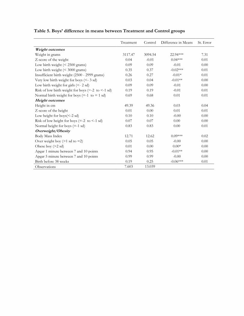
Table 5. Boys’ difference in means between Treatment and Control groups

Treatment Control Difference in Means St. Error

Weight outcomes Weight in grams 3117.47 3094.54 22.94*** 7.31

Z-score of the weight 0.04 -0.01 0.04*** 0.01

Low birth weight (< 2500 grams) 0.09 0.09 -0.01 0.00

Low birth weight (< 3000 grams) 0.35 0.37 -0.02*** 0.01

Insufficient birth weight (2500 - 2999 grams) 0.26 0.27 -0.01* 0.01

Very low birth weight for boys (<- 3 sd) 0.03 0.04 -0.01** 0.00

Low birth weight for girls (<- 2 sd) 0.09 0.09 -0.01 0.00

Risk of low birth weight for boys (=-2 to <-1 sd) 0.19 0.19 -0.01 0.01

Normal birth weight for boys (=-1 to = 1 sd) 0.69 0.68 0.01 0.01

Height outcomes Height in cm 49.39 49.36 0.03 0.04

Z-score of the height 0.01 0.00 0.01 0.01

Low height for boys(<-2 sd) 0.10 0.10 -0.00 0.00

Risk of low height for boys (=-2 to <-1 sd) 0.07 0.07 0.00 0.00

Normal height for boys (=-1 sd) 0.83 0.83 0.00 0.01

Overweight/Obesity Body Mass Index 12.71 12.62 0.09*** 0.02

Over weight boy (>1 sd to =2) 0.05 0.05 -0.00 0.00

Obese boy (>2 sd) 0.01 0.00 0.00* 0.00

Apgar 1 minute between 7 and 10 points 0.94 0.95 -0.01** 0.00

Apgar 5 minute between 7 and 10 points 0.99 0.99 -0.00 0.00

Birth before 38 weeks 0.19 0.25 -0.06*** 0.01

Observations 7.603 13.039

Table 6. Boys’ descriptive statistics by treatment status

Treatment Control Difference in Means St. Error

Married or cohabitating 0.34 0.50 -0.16*** 0.01

Disabled 0.01 0.00 0.00** 0.00

Attending school 0.23 0.15 0.08*** 0.01

Years of schooling 8.05 9.83 -1.77*** 0.04

No education 0.01 0.01 0.01*** 0.00

Primary school 0.24 0.12 0.12*** 0.01

Secondary school 0.71 0.72 -0.01 0.01

Technical education 0.02 0.09 -0.06*** 0.00

Degree 0.01 0.06 -0.06*** 0.00

Post-degree 0.00 0.00 -0.00*** 0.00

No activity 0.16 0.08 0.08*** 0.00

Working 0.15 0.34 -0.19*** 0.01

Looking for a job 0.04 0.04 0.01* 0.00

Studying 0.23 0.14 0.09*** 0.01

Several tasks 0.42 0.40 0.02*** 0.01

Retired 0.00 0.00 -0.00** 0.00

Household size 1.07 1.05 0.03*** 0.00

Monthly income 38398.71 141861.20 -103462.49*** 4089.45

Income -missing information 0.86 0.71 0.15*** 0.01

Number of prenatal appointments 6.42 6.76 -0.34*** 0.03

Number of prenatal appointments missing 0.01 0.02 -0.01*** 0.00

Stratum 0 0.00 0.00 0.00** 0.00

Stratum 1 0.37 0.19 0.18*** 0.01

Stratum 2 0.54 0.53 0.01 0.01

Stratum 3 0.09 0.28 -0.19*** 0.01

Stratum 4 0.00 0.00 -0.00*** 0.00

SISBEN score below 48 0.78 0.58 0.19*** 0.01

Months registered after birth 0.09 0.05 0.04*** 0.00

Months registered after birth – missing 0.43 0.64 -0.21*** 0.01

Certified by a doctor 0.99 0.98 0.01*** 0.00

Twins 0.00 0.00 0.00 0.00

Twins category – missing 0.98 0.98 0.01** 0.00

Labor spontaneous 0.68 0.56 0.11*** 0.01

Labor cesarean 0.29 0.37 -0.08*** 0.01

Labor instrumented 0.03 0.06 -0.03*** 0.00

Labor attended by a doctor 1.00 1.00 0.00 0.00

Father’s age 27.96 29.35 -1.39*** 0.11

Father’s without education 0.01 0.00 0.00*** 0.00

Father’s educational level: primary 0.09 0.04 0.05*** 0.00

Father’s educational level: vocational 0.32 0.21 0.11*** 0.01

Father’s educational level: technical 0.02 0.03 -0.01*** 0.00

Father’s educational level: degree 0.03 0.03 -0.01** 0.00

Father’s educational level: missing 0.53 0.68 -0.15*** 0.01

Owned house 0.40 0.35 0.05*** 0.01

Health insurance subsidized 0.76 0.32 0.44*** 0.01

Without health insurance 0.17 0.14 0.03*** 0.01

Contribute to health insurance 0.07 0.54 -0.48*** 0.01

Year of birth: 2009 0.15 0.42 -0.26*** 0.01

Year of birth: 2010 0.45 0.29 0.17*** 0.01

Observations 7.603 13.039

Table 7. Girls’ descriptive statistics by Treatment Status

Treatment Control Difference in Means St. Error

Married or cohabitating 0.33 0.51 -0.18*** 0.01

Disabled 0.01 0.00 0.00** 0.00

Attending school 0.24 0.16 0.08*** 0.01

Years of schooling 8.12 9.80 -1.69*** 0.05

No education 0.02 0.01 0.01*** 0.00

Primary school 0.22 0.12 0.10*** 0.01

Secondary school 0.73 0.71 0.01 0.01

Technical education 0.03 0.09 -0.06*** 0.00

Degree 0.01 0.06 -0.05*** 0.00

Post-degree 0.00 0.00 -0.00*** 0.00

No activity 0.16 0.08 0.08*** 0.00

Working 0.14 0.34 -0.20*** 0.01

Looking for a job 0.05 0.04 0.01*** 0.00

Studying 0.24 0.14 0.10*** 0.01

Several tasks 0.42 0.41 0.01 0.01

Retired 0.00 0.00 -0.00*** 0.00

Household size 1.07 1.05 0.02*** 0.00

Monthly income 37216.32 140319.33 -103103.02*** 3749.18

Income -missing information 0.86 0.72 0.14*** 0.01

Number of prenatal appointments 6.44 6.80 -0.36*** 0.04

Number of prenatal appointments missing 0.01 0.03 -0.01*** 0.00

Stratum 0 0.00 0.00 0.00** 0.00

Stratum 1 0.37 0.19 0.18*** 0.01

Stratum 2 0.54 0.53 0.01 0.01

Stratum 3 0.09 0.28 -0.19*** 0.01

Stratum 4 0.00 0.00 -0.00** 0.00

SISBEN score below 48 0.77 0.57 0.20*** 0.01

Months registered after birth 0.09 0.05 0.04*** 0.00

Months registered after birth – missing 0.43 0.64 -0.21*** 0.01

Certified by a doctor 0.98 0.98 0.01*** 0.00

Twins 0.00 0.00 0.00 0.00

Twins category – missing 0.98 0.98 0.00** 0.00

Labor spontaneous 0.70 0.59 0.11*** 0.01

Labor cesarean 0.27 0.34 -0.07*** 0.01

Labor instrumented 0.03 0.06 -0.03*** 0.00

Labor attended by a doctor 1.00 1.00 0.00 0.00

Father’s age 27.97 29.35 -1.38*** 0.12

Father’s without education 0.01 0.00 0.00*** 0.00

Father’s educational level: primary 0.09 0.04 0.05*** 0.00

Father’s educational level: vocational 0.32 0.21 0.11*** 0.01

Father’s educational level: technical 0.02 0.03 -0.01*** 0.00

Father’s educational level: degree 0.03 0.03 -0.01** 0.00

Father’s educational level: missing 0.53 0.69 -0.15*** 0.01

Owned house 0.39 0.35 0.04*** 0.01

Health insurance subsidized 0.77 0.32 0.45*** 0.01

Without health insurance 0.17 0.14 0.03*** 0.01

Contribute to health insurance 0.06 0.54 -0.47*** 0.01

Year of birth: 2009 0.16 0.42 -0.26*** 0.01

Year of birth: 2010 0.45 0.28 0.17*** 0.01

Observations 7.244 12.264

Table 8. Impact of the program Buen Comienzo on Birth Outcomes among Girls

Treatment 1 Treatment 2 Treatment 3 Treatment 4

Dependent variable

Z-score of Birth Weight 0.057 *** 0.193 *** 0.007

0.230 ***

(0.021)

(0.028)

(0.034)

(0.036)

Low Birth Weight (LBW) -0.012 *** -0.037 *** -0.001

-0.046 ***

(0.006)

(0.007)

(0.009)

(0.009)

Very Low Birth Weight -0.014 *** -0.031 *** 0.003

-0.028 ***

(0.003)

(0.004)

(0.006)

(0.005)

At risk of LBW -0.005

-0.022 ** -0.020

-0.024 *

(0.008)

(0.012)

(0.013)

(0.014)

Insufficient Birth Weight -0.010

-0.007

-0.030 * -0.008

(0.01)

(0.014)

(0.016)

(0.018)

Normal Weight 0.012

0.048 *** 0.018

0.054 ***

(0.01)

(0.014)

(0.016)

(0.017)

Birth Weight<2.5 -0.007

-0.044 *** 0.008

-0.054 ***

(0.006)

(0.009)

(0.01)

(0.011)

Birth Weight<1.5 -0.006 *** -0.015 *** 0.002

-0.011 ***

(0.002)

(0.003)

(0.004)

(0.004)

Z-score size (cm) 0.047 *** 0.159 *** -0.003

0.195 ***

(0.02)

(0.028)

(0.033)

(0.035)

Short -0.014 *** -0.038 *** 0.006

-0.046 ***

(0.006)

(0.007)

(0.009)

(0.009)

At risk of being short 0.005

0.002

-0.020 * 0.006

(0.008)

(0.01)

(0.012)

(0.013)

Normal Size 0.008

0.034 *** 0.013

0.039 ***

(0.009)

(0.012)

(0.014)

(0.015)

Size <45 cm -0.014 *** -0.038 *** 0.006

-0.046 ***

(0.006) (0.007) (0.009) (0.009)

18911 13994 13654 12931

Notes: *, **, ***, refers to 10%, 5%, and 1% levels of significance, respectively. We include LBW and having a

birth weight below 2.500gr as separated outcomes. We did this because in the case of girls, LBW defined as a BW

2SD below the average population, is being below 2.400gr. In the case of boys both indicators are the same.

Similarly, Low height and being shorter than 45cm are included as different outcomes. This was because in the

case of boys, having low height is defined as being shorter than 46cm. In the case of girls, both indicators are the

same. Among the covariates included there are the child’s mother’s characteristics such as age, marital status,

disability, school attendance, number of years of education, education level, indicators for economic activity,

health insurance and multiple births: We also include as covariates household size, household income, strata,

father’s education, housing.

Table 9. Impact of the program Buen Comienzo on Birth Outcomes among Boys

Treatment 1 Treatment 2 Treatment 3 Treatment 4

Dependent variable Z-score of Birth Weight 0.006

0.088 *** -0.098 *** 0.090 ***

(0.02)

(0.027)

(0.033)

(0.034)

Low Birth Weight (LBW) 0.003

-0.021 *** 0.024 *** -0.026 ***

(0.006)

(0.007)

(0.01)

(0.009)

Very Low Birth Weight -0.002

-0.022 *** 0.018 *** -0.027 ***

(0.004)

(0.004)

(0.006)

(0.005)

At risk of LBW -0.006

-0.011

0.011

-0.002

(0.008)

(0.011)

(0.013)

(0.015)

Insufficient Birth Weight -0.003

-0.006

0.013

0.002

(0.009)

(0.013)

(0.014)

(0.017)

Normal Weight 0.005

0.036 *** -0.024

0.036 ***

(0.009)

(0.014)

(0.015)

(0.017)

Birth Weight<2.5 0.003

-0.021 *** 0.024 *** -0.026 ***

(0.006)

(0.007)

(0.01)

(0.009)

Birth Weight<1.5 -0.005 *** -0.015 *** 0.007 * -0.014 ***

(0.002)

(0.002)

(0.004)

(0.003)

Z-score size (cm) -0.017

0.065 *** -0.132 *** 0.091 ***

(0.02)

(0.026)

(0.034)

(0.033)

Short -0.003

-0.027 *** 0.018 * -0.038 ***

(0.006)

(0.008)

(0.01)

(0.01)

At risk of being short 0.014 *** 0.018 *** 0.013

0.011

(0.005)

(0.007)

(0.008)

(0.009)

Normal Size -0.011

0.009

-0.033 *** 0.025 ***

(0.008)

(0.01)

(0.012)

(0.013)

Size <45 cm -0.002

-0.024

0.022 *** -0.026 ***

(0.005)

(0.006)

(0.008)

(0.007)

20012 14797 14529 13654 Notes: *, **, ***, refers to 10%, 5%, and 1% levels of significance, respectively. We include LBW and having a

birth weight below 2.500gr as separated outcomes. We did this because in the case of girls, LBW defined as a BW

2SD below the average population, is being below 2.400gr. In the case of boys both indicators are the same.

Similarly, Low height and being shorter than 45cm are included as different outcomes. This was because in the

case of boys, having low height is defined as being shorter than 46cm. In the case of girls, both indicators are the

same. Among the covariates included there are the child’s mother’s characteristics such as age, marital status,

disability, school attendance, number of years of education, education level, indicators for economic activity,

health insurance and multiple births: We also include as covariates household size, household income, strata,

father’s education, housing.

Table 10. Pre-term Birth

Treatment 1 Treatment 2 Treatment 3 Treatment 4

Boys

Girls

Boys

Girls

Boys

Girls

Boys

Girls

Being born -0.036 *** -0.036 *** -0.065 *** -0.080 *** 0.005

-0.002

-0.073 *** -0.087 ***

before week 38 (0.008) (0.008) (0.011) (0.012) (0.013) (0.014) (0.014) (0.015)

Note: *, **, *** corresponds to the 10%, 5% and 1% level of significance, respectively. Among the covariates

included there are the child’s mother’s characteristics such as age, marital status, disability, school attendance,

number of years of education, education level, indicators for economic activity, health insurance and multiple

births: We also include as covariates household size, household income, strata, father’s education, housing.

Table 11. Covariate balance after the matching

Girls Boys

Control Treatment 1

Diff. In means

Control Treatment

1 Diff. In means

Married or cohabitating 0.33 0.37 -0.04*** 0.34 0.37 -0.03***

Disabled 0.01 0.01 0.00 0.00 0.00 0.00

Attend school 0.24 0.23 0.01*** 0.23 0.22 0.01***

Years of schooling 8.14 8.52 -0.38*** 8.08 8.46 -0.37***

Primary school 0.22 0.20 0.02*** 0.24 0.22 0.02***

Secondary school 0.73 0.76 -0.03*** 0.72 0.75 -0.03***

Technical education 0.03 0.02 0.00 0.02 0.02 0.00**

Degree 0.01 0.01 0.00 0.01 0.01 0.00

Post-degree 0.00 0.00 0.00 0.00 0.00 0.00

Working 0.14 0.15 -0.00 0.15 0.15 -0.00

Looking for a job 0.05 0.04 0.00 0.04 0.04 0.00

Studying 0.24 0.23 0.01*** 0.23 0.22 0.01*

Several tasks 0.42 0.44 -0.03*** 0.42 0.45 -0.03***

Retired 0.00 0.00 0.00 0.00 0.00 0.00

Household size 1.07 1.04 0.03*** 1.07 1.04 0.03***

Monthly income 37277.99 42162.70 -4884.72*** 39099.99 43174.63 -4074.64***

Income -missing information

0.86 0.88 -0.02*** 0.86 0.88 -0.02***

Stratum 1 0.37 0.32 0.04*** 0.37 0.34 0.03***

Stratum 2 0.54 0.58 -0.04*** 0.54 0.57 -0.04***

Stratum 3 0.09 0.10 -0.01*** 0.09 0.09 0.00

Stratum 4 0.00 0.00 0.00 0.00 0.00 0.00

Sisben score below 48 0.77 0.77 0.01 0.77 0.77 0.00

Twins 0.01 0.01 0.00 0.00 0.00 0.00

Twins category – missing 0.98 0.98 -0.00 0.98 0.98 -0.00

Father’s age 27.97 27.50 0.46*** 27.96 27.46 0.50***

Father’s without education 0.01 0.01 0.00 0.01 0.01 0.00

Father’s educational level: primary 0.09 0.08 0.01*** 0.09 0.09 0.01***

Father’s educational level: vocational 0.34 0.32 0.02*** 0.34 0.32 0.02***

Father’s educational level: technical 0.02 0.02 0.00 0.02 0.02 0.00

Father’s educational level: degree 0.03 0.03 0.00 0.03 0.03 0.00

Father’s educational level: missing 0.52 0.54 -0.03*** 0.52 0.54 -0.03***

Owned house 0.39 0.36 0.03*** 0.39 0.36 0.04***

Without health insurance 0.17 0.14 0.03*** 0.17 0.14 0.03***

Contribute to health insurance 0.07 0.23 -0.17*** 0.07 0.23 -0.17***

Year of birth: 2009 0.15 0.22 -0.07*** 0.15 0.22 -0.07***

Year of birth: 2010 0.45 0.34 0.10*** 0.45 0.36 0.09***

Mother's age 23.56 23.74 -0.18*** 23.52 23.64 -0.11**

Birth Month 2 0.07 0.06 0.00 0.06 0.06 0.00

Birth Month 3 0.08 0.08 0.00 0.08 0.08 0.00

Birth Month 4 0.07 0.07 0.00 0.07 0.07 0.00

Birth Month 5 0.07 0.07 0.00 0.07 0.07 0.00

Birth Month 6 0.06 0.06 0.00 0.06 0.06 0.00

Birth Month 7 0.07 0.06 0.00 0.07 0.07 -0.00

Birth Month 8 0.09 0.09 0.00 0.09 0.09 0.00

Birth Month 9 0.10 0.10 0.00 0.11 0.11 0.00

Birth Month 10 0.11 0.11 -0.00 0.11 0.11 0.00

Birth Month 11 0.10 0.10 -0.00 0.10 0.10 0.00

Birth Month 12 0.11 0.11 0.00 0.11 0.11 -0.00

Sisben Score 35.20 37.17 -1.97*** 35.12 36.88 -1.76***

Note: *, **, *** corresponds to the 10%, 5% and 1% level of significance, respectively. The average values

correspond to the matched observations using treatment group 1, four matches and correcting by bias.

Table 12. Cost-benefit estimates

Concept

Para

mete

rs Treatment 1 Treatment 2 Treatment 3 Treatment 4

Boys Girls Boys Girls Boys Girls Boys Girls

(1) (2) (3) (4) (5) (6) (7) (8)

Benefits

1. Birthweight* 0.0 0.0 85.3 229.9 -128.6 0.0 103.7 284.5

Impact Estimate

Weight below 2500 gr 0.003

-0.007

-0.021 *** -0.044 *** 0.024 *** 0.008 (0) -0.026 *** -0.054 ***

(0.006)

(0.006)

(0.007)

(0.009)

(0.01)

(0.01) (0.009)

(0.011)

Discount Rate 5.0%

1. Reducing Infant Mortality

Drop in probability of infant death for moving from 2.00-2.49 kg to 2.50-2.99 kg

7.8%

Cost of saving a life (USD$2012) 1,520

0.8

2.4

4.9

-2.8

2.9

6.1 Years Discounted 1

2. Reducing Neonatal Medical Attention

Estimated Costs per Child born weighing <2.5 kg 255

1.7

4.9

10.1

-5.7

5.9

12.6 90% born at hospital, 10% at home 0

Home costs=10% hospital costs

3. Reducing Costs of Illnesses and Medical Care for Infants and Children Due to LBW

Cost per child under 2.5 kg 48

0.3

1.0

2.0

-1.1

1.2

2.5 Years Discounted 1

4. Reducing Lifetime Productivity due to Stunting

Share of Annual Earnings 2.2%

8

22

46

(25)

27

56 Expected Annual Earnings 2500

Years Discounted 60

5. Increase in Lifetime Productivity due to Increased Ability Due to Reduction of LBW

Share of Annual Earnings (7.5%-2.2%) 5.3%

18

53

110

(61)

64

136 Years Discounted 60

6. Reducing Costs of Chronic Diseases Due to LBW

Reduction in the Prob of Chronic Disease 8.7%

1

2

5

-3

3

6 Number of Years of Earnings 10

7. Cross-Generational Impacts of LBW 0.0 0.0 0.0 52.4 -29.3 0.0 0.0 64.9

2. Height* 0 177 245 603 -499 0 343 740

Impact Estimate

Z-score Height -0.017

0.047 *** 0.065 *** 0.159 *** -0.132 *** -0.003 0.091 *** 0.195 ***

(0.02) (0.02) (0.026) (0.028) (0.034) (0.033) (0.033) (0.035)

Increase in Lifetime Earnings 0

177

245

603

-499

0

343

740 2% per 0.25 SD increase 2.0%

Years Discounted 60

Total Benefits 0 177 330 833 -628 0 447 1024

Costs 163.5 163.5 163.5 163.5 65.4 65.4 163.5 163.5

Unitary Cost Per Month 22

Number Of Months 7.5

7.5

7.5

7.5

3.0

3.0

7.5

7.5

Benefit/Cost 0.00 1.08 2.02 5.10 -9.60 0.00 2.74 6.27

Note: * Assumptions based on Behrman, Alderman and Hoddinott (2004).

References

Alberto Abadie and Guido W. Imbens. Simple and bias-corrected matching estimators for average treatment effects. NBER TechnicalWorking Papers 0283, National Bureau of Economic Research, Inc, October 2002. Harold Alderman, Jere R. Behrman, Victor Lavy, and Rekha Menon. Child health and school enrollment: A longitudinal analysis. The Journal of Human Resources, 36(1):pp. 185-205, 2001. Harold Alderman, John Hoddinott, and Bill Kinsey. Long-term consequences of early childhood malnutrition. FCND discussion papers 168, International Food Policy Research Institute (IFPRI), 2003. Douglas Almond, Kenneth Y. Chay, and David S. Lee. The costs of low birth weight. The Quarterly Journal of Economics, 120(3):1031-1083, 2005. Douglas Almond, Joseph J. Doyle, Amanda E. Kowalski, and Heidi Williams. Estimating marginal returns to medical care: Evidence from at-risk newborns. The Quarterly Journal of Economics, 125(2):591-634, 2010. Douglas Almond, Hilary W. Hoynes, and Diane Whitmore Schanzenbach. Inside the war on poverty: The impact of food stamps on birth outcomes. The Review of Economics and Statistics, 93(2):387-403, December 2011. Verónica Amarante & Marco Manacorda & Edward Miguel & Andrea Vigorito, 2016."Do Cash Transfers Improve Birth Outcomes? Evidence from Matched Vital statistics, Program, and Social Security Data," American Economic Journal: Economic Policy, American Economic Association, vol. 8(2), pages 1-43, May. Jere R. Behrman, Harold Alderman, and John Hoddinott. “Hunger and Malnutrition” Copenhagen Consensus Challenge Paper, May 2004. Jere R. Behrman and Mark R. Rosenzweig. Returns to birthweight. The Review of Economics and Statistics, 86(2):586-601, 06 2004. Jere R. Behrman, Yingmei Cheng, and Petra E. Todd. Evaluating Preschool Programs When Length of Exposure to the Program Varies: A Nonparametric Approach. The Review of Economics and Statistics, 86(1):108-132, February 2004. Raquel Bernal and Adriana Camacho. La importancia de los programas para la primera infancia en Colombia. DOCUMENTOS CEDE 007605, UNIVERSIDAD DE LOS ANDES-CEDE, July 2010. AT Bhutta, MA Cleves, PH Casey, MM Cradock, and KS Anand. Cognitive and behavioral outcomes of school-aged children who were born preterm: A meta-analysis. JAMA, 288(6):728-737, 2002.

Marianne P. Bitler and Janet Currie. Does WIC work? the effects of WIC on pregnancy and birth outcomes. Journal of Policy Analysis and Management, 24(1):73-91, 2005. Maureen M. Black. Micronutrient deficiencies and cognitive functioning. The Journal of Nutrition, 133(11):3927S-3931S, 2003. Robert E. Black. Micronutrients in pregnancy. British Journal of Nutrition, 85: S193-S197, 5 2001. ISSN 1475-2662. Sandra E. Black, Paul J. Devereux, and Kjell Salvanes. From the cradle to the labor market? the effect of birth weight on adult outcomes. NBER Working Papers 11796, National Bureau of Economic Research, Inc, November 2005. Richard Blundell and Monica Costa Dias. Alternative approaches to evaluation in empirical microeconomics. Journal of Human Resources, 44(3):565-640, Jun 2009. Marco Caliendo. Microeconometric Evaluation of Labour Market Policies. Springer, 2006. Anne Case and Christian Paxson. Children's health and social mobility. The Future of Children, 6:151-173, 2006. Resul Cesur and Inas Rashad. High birth weight and cognitive outcomes. NBER Working Papers 14524, National Bureau of Economic Research, Inc, December 2008. Paul Contoyannis and Martin Dooley. The role of child health and economic status in educational, health, and labour market outcomes in young adulthood. Canadian Journal of Economics, 43(1):323-346, February 2010. Flavio Cunha and James J. Heckman. The economics and psychology of inequality and human development. Journal of the European Economic Association, 7(2-3): 320-364, 04-05 2009. Janet Currie. Inequality at birth: Some causes and consequences. American Economic Review, 101(3):1-22, May 2011. Janet Currie and W. Bentley MacLeod. First do no harm? tort reform and birth outcomes. The Quarterly Journal of Economics, 123(2):795-830, 05 2008. Suzanne Duryea, A. Olgiati and L. Stone (2006), “Registro inexacto de nacimientos en América Latina”, RES Working Papers, 4444, Inter-American Development Bank, Research Department. Washington DC. Johan G.,Eriksson, Kajantie, E., Osmond, C., Thornburg, K. and Barker, D. J.P. (2010), Boys live dangerously in the womb. Am. J. Hum. Biol., 22: 330–335. Jason M. Fletcher. The medium term schooling and health effects of low birth weight: Evidence from siblings. Economics of Education Review, 30(3):517-527, June 2011.

Paul Glewwe and Hanan G Jacoby. An economic analysis of delayed primary school enrollment in a low income country: The role of early childhood nutrition. The Review of Economics and Statistics, 77(1):156-69, February 1995. Paul Glewwe, Hanan G. Jacoby, and Elizabeth M. King. Early childhood nutrition and academic achievement: a longitudinal analysis. Journal of Public Economics, 81(3):345-368, September 2001. Catherine Haeck and Pierre Lefebvre. A Simple Recipe: the Effect of a Prenatal Nutrition Program on Child Health at Birth. Forthcoming, Labour Economics, 2016. James Heckman and Edward Vytlacil. Identifying the role of cognitive ability in explaining the level of and change in the return to schooling. The Review of Economics and Statistics, 83(1):1-12, February 2001. James J. Heckman. The economics, technology and neuroscience of human capability formation. NBER Working Papers 13195, National Bureau of Economic Research, Inc, June 2007. James J Heckman, Hidehiko Ichimura, and Petra E Todd. Matching as an econometric evaluation estimator: Evidence from evaluating a job training programme. Review of Economic Studies, 64(4):605-54, October 1997. James J Heckman, Hidehiko Ichimura, and Petra Todd. Matching as an econometric evaluation estimator. Review of Economic Studies, 65(2):261-94, April 1998. Hilary W. Hoynes, Marianne E. Page, and Ann Huff Stevens. Is a WIC start a better start? evaluating wics impact on infant health using program introduction. NBER Working Papers 15589, National Bureau of Economic Research, Inc, December 2009. Hilary W. Hoynes, Douglas L. Miller, and David Simon. Income, the earned income tax credit, and infant health. NBER Working Papers 18206, National Bureau of Economic Research, Inc, July 2012. Guido W. Imbens. Nonparametric estimation of average treatment effects under exogeneity: A review. The Review of Economics and Statistics, 86(1):4-29, February 2004. Rucker C Johnson and Robert F Schoeni. The influence of early-life events on human capital, health status, and labor market outcomes over the life course. The B.E. Journal of Economic Analysis & Policy, 11(3):1-57, September 2011. Ida Kirkegaard, Carsten Obel, Morten Hedegaard, and Tine Brink Henriksen. Gestational age and birth weight in relation to school performance of 10-year-old children: A follow-up study of children born after 32 completed weeks. Pediatrics, 118(4):1600-1606, 2006. MS Kramer. Determinants of low birth weight : methodological assessment and meta-analysis. Bulletin of World Health Organisation, 65:663737, 1987.

D. Lawlor, G. Davey Smith, H. Clark, and D. Leon. The associations of birthweight, gestational age and childhood bmi with type 2 diabetes: findings from the Aberdeen children of the 1950s cohort. Diabetologia, 49:2614-2617, 2006. H J McArdle and C J Ashworth. Micronutrients in fetal growth and development. British medical bulletin, 55(3):499-510, 1999. Anne M Molloy, Peadar N Kirke, Lawrence C Brody, John M Scott, and James L Mills. Effects of folate and vitamin b12 deficiencies during pregnancy on fetal, infant, and child development. Food and nutrition bulletin, 29(2 Suppl):S101-S111; discussion S112-S115, 2008. Philip Oreopoulos, Mark Stabile, RandyWalld, and Leslie L. Roos. Short-, medium-, and long-term consequences of poor infant health: An analysis using siblings and twins. Journal of Human Resources, 43(1):88-138, 2008. Kaja Rahu, Mati Rahu, Helle Pullmann, and Jri Allik. Effect of birth weight, maternal education and prenatal smoking on offspring intelligence at school age. Early Human Development, 86:493-497, 2010. A. D. Roy. Some thoughts on the distribution of earnings. Oxford Economic Papers, 3(2):135-146, 1951. Heather Royer. Separated at girth: Us twin estimates of the effects of birth weight. American Economic Journal: Applied Economics, 1(1):49-85, January 2009. Donald Rubin. Bayesian inference for causal effects. The Annals of Statistics, 6: 34-58, 1978. Henrik Toft Sorensen, Svend Sabroe, Jorn Olsen, Kenneth J Rothman, Matthew W Gillman, and Peer Fischer. Birth weight and cognitive function in young adult life: historical cohort study. BMJ, 315(7105):401-403, 8 1997.

Appendix

Figure A.1 Probability of being treated by SISBEN Score

Table A.1. Descriptive Statistics for Girls: differences in mean outcomes between the

Treatment and Control groups under analysis. SISBEN 1 & 2

SISBEN 1 and 2 SISBEN 3

Treatment Control

Diff. In Means

Treatment Control Diff. In Means

Weight outcomes

Weight in grams 3018.82 2987.83 30.99*** 3029.90 3010.85 19.05

Z-score of the weight 0.03 -0.03 0.06*** 0.06 0.02 0.04

Low birth weight (< 2500 grams) 0.11 0.12 -0.01* 0.11 0.11 0.00

Low birth weight (< 3000 grams) 0.44 0.47 -0.02*** 0.43 0.45 -0.01

Insufficient birth weight (2500 - 2999 grams)

0.34 0.35 -0.01 0.32 0.34 -0.01

Very low birth weight (<- 3 sd) 0.02 0.03 -0.01*** 0.02 0.03 -0.01**

Low birth weight (<- 2 sd) 0.07 0.09 -0.01** 0.08 0.08 -0.00

Risk of low birth weight (=-2 to <-1 sd) 0.20 0.21 -0.01 0.18 0.19 -0.01

Normal birth weight (=-1 to = 1 sd) 0.68 0.66 0.02* 0.68 0.68 0.00

Height outcomes

Height in cm 48.92 48.76 0.16*** 48.99 48.87 0.12

Z-score of the height 0.03 -0.03 0.06*** 0.05 0.01 0.04

Low height (<-2 sd) 0.07 0.09 -0.02*** 0.07 0.08 -0.01*

Risk of low height (=-2 to <-1 sd) 0.16 0.16 0.00 0.14 0.14 -0.00

Normal height (=-1 sd) 0.78 0.76 0.02** 0.79 0.78 0.02

Over weight child(>1 sd to =2) 0.05 0.05 0.00 0.06 0.05 0.01

Obese child (>2 sd) 0.01 0.01 -0.00 0.01 0.01 -0.00

APGAR 1 minute between 7 and 10 points 0.96 0.95 0.01 0.95 0.97 -0.01*

APGAR 5 minute between 7 and 10 points 0.99 0.99 0.00 0.99 0.99 -0.00

Birth before 38 weeks 0.18 0.23 -0.05*** 0.18 0.23 -0.04***

Observations 12637 6907

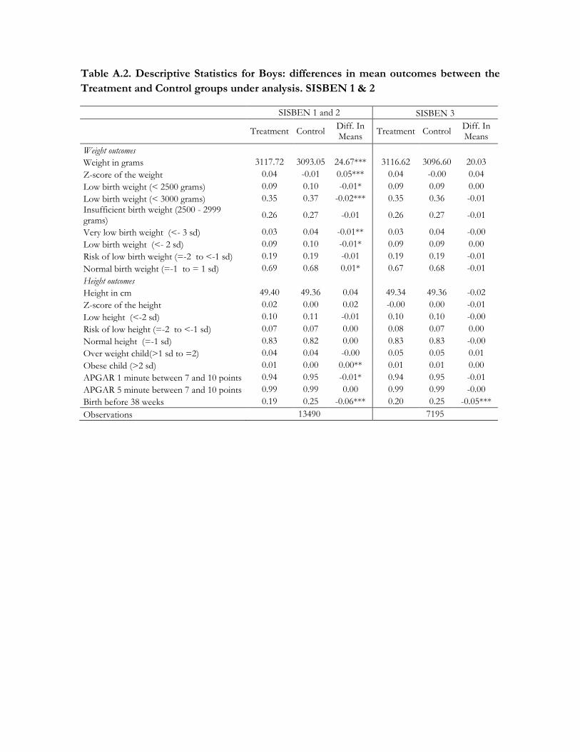
Table A.2. Descriptive Statistics for Boys: differences in mean outcomes between the

Treatment and Control groups under analysis. SISBEN 1 & 2

SISBEN 1 and 2 SISBEN 3

Treatment Control

Diff. In Means

Treatment Control Diff. In Means

Weight outcomes

Weight in grams 3117.72 3093.05 24.67*** 3116.62 3096.60 20.03

Z-score of the weight 0.04 -0.01 0.05*** 0.04 -0.00 0.04

Low birth weight (< 2500 grams) 0.09 0.10 -0.01* 0.09 0.09 0.00

Low birth weight (< 3000 grams) 0.35 0.37 -0.02*** 0.35 0.36 -0.01

Insufficient birth weight (2500 - 2999 grams)

0.26 0.27 -0.01 0.26 0.27 -0.01

Very low birth weight (<- 3 sd) 0.03 0.04 -0.01** 0.03 0.04 -0.00

Low birth weight (<- 2 sd) 0.09 0.10 -0.01* 0.09 0.09 0.00

Risk of low birth weight (=-2 to <-1 sd) 0.19 0.19 -0.01 0.19 0.19 -0.01

Normal birth weight (=-1 to = 1 sd) 0.69 0.68 0.01* 0.67 0.68 -0.01

Height outcomes

Height in cm 49.40 49.36 0.04 49.34 49.36 -0.02

Z-score of the height 0.02 0.00 0.02 -0.00 0.00 -0.01

Low height (<-2 sd) 0.10 0.11 -0.01 0.10 0.10 -0.00

Risk of low height (=-2 to <-1 sd) 0.07 0.07 0.00 0.08 0.07 0.00

Normal height (=-1 sd) 0.83 0.82 0.00 0.83 0.83 -0.00

Over weight child(>1 sd to =2) 0.04 0.04 -0.00 0.05 0.05 0.01

Obese child (>2 sd) 0.01 0.00 0.00** 0.01 0.01 0.00

APGAR 1 minute between 7 and 10 points 0.94 0.95 -0.01* 0.94 0.95 -0.01

APGAR 5 minute between 7 and 10 points 0.99 0.99 0.00 0.99 0.99 -0.00

Birth before 38 weeks 0.19 0.25 -0.06*** 0.20 0.25 -0.05***

Observations 13490 7195

ogotá -