An asymptotic-parallel-in-time method for weather and climate prediction

Beth Wingate University of Exeter

Terry Haut Los Alamos National Laboratory

Jared Whitehead Brigham Young University

Outline

o  A brief introduction to parallel-in-time

o  Describe a locally asymptotic slow solution

o  Show some results from the shallow water equations

o  Summarize and lead into highly parallel linear propagators

The early days of computational science

Slow Dynamics L.F. Richardson in (1922) - using ‘computers’ (us)

Charney (1948) and Charney (1950) - derived ‘slow’ or Quasi-Geostrophic (QG) equations (important conceptual model)

Charney and Phillips (1953) – the first realistic numerical weather prediction using the QG eqs

L.F. Richardson

J. Charney J. von Neumann

And then our community proceeded to not use QG for weather prediction.

We have been dealing with strategies for overcoming or managing small time steps ever since.

Characteristics of emerging computer architectures

o  Unprecedented parallelism: Current High Performance computers can scale up to 250,000 processors. Efficient use of new architectures will require we know how to scale up to 1 Billion parallel processors.

o  Processors speeds will not be significantly faster than current processors.

o  Memory per processor limited.

o  We will have a greater need to have fault-tolerant algorithms

o  We will have to understand asynchronous computing

Algorithms and new computing architectures

o  Fixed grid on N processors

For a fixed grid you may have an optimal distribution of the grid on N processors, then the only dimension left available for parallelization is time.

o  Grid refinement (we’ll still have to wait for each time step) Because current algorithms need to reduce their maximum time step as the number of grid points increases, these new machines may not significantly reduce wall clock time . You may be able to have a higher resolution grid but you will still wait a longer time for each time step to complete.

From a wall-clock-time point of view, current models may appear to dissipate into the machine.

See Jean Côté’s talk from PDEs on the Sphere Cambridge at http://www.newton.ac.uk/programmes/AMM/seminars/2012092814201.html

Graphical representation of the parallel-in-time algorithm

Nievergelt, 1964 Lions, Maday, Turinici, 2001

Successful for dissipative stiffness

Oscillatory Stiffness in Parareal

The roots of the locally asymptotic slow/coarse solution

Slow Manifolds (nonlinear normal mode initialization, center manifolds, dynamical systems, etc)

Machanauer (1977), Baer (1877), Tribbia ( 1979), etc

Leith, Nonlinear Normal Mode Initialization and Quasi-Geostrophic Theory (1980)

Lorenz, On the Existence of a Slow Manifold (1986)

Lorenz and Krishnamurthy, On the non-Existence of the Slow Manifold (1987)

Lorenz, The Slow Manifold – what is it? (1991)

(….so far the answer is ‘it is a fuzzy manifold’.)

Ed Lorenz Chuck Leith

PDEs with oscillatory stiffness – the equations of climate and weather

•  The operator results in temporal oscillations on a time scale of

•  Standard numerical time-stepping methods must use time steps

Embid and Majda, 1996, 1998, Majda and Embid, 1998, Schochet, 1994, Klainerman and Majda 1981, Wingate, Embid, Holmes-Cerfon, Taylor, 2011

One way to view the problem (also used for exponential integrators)

v varies slower than u, but v still has some oscillations

An asymptotic method-of-multiple scales in time (another way to derive Quasi Geostrophy is a singular perturbation in time):

Asymptotic solution looks like:

Embid and Majda, 1996, 1998, Majda and Embid, 1998, Schochet, 1994, Klainerman and Majda 1981, Wingate, Embid,, Cerfon-Holme Taylor, 2011

Over a few oscillations we approximate the time integral using HMM:

Test of the method on the shallow water equations

Example of the solution in time: epsilon=.01, Delta T = .3

�T

Relative L∞ errors for epsilon=10^{-1} , using the asymptotic based parallel-in-time integrator and taking Delta T=3/10 and Delta t=1/500 . Each graph is for fixed a iteration k (1,3,5 ), and the errors are plotted as a function of the time n Delta T , n=1..N . The errors are shown on a log10 scale.

Maximum relative error versus number of iterations

APAR: 5 Parareal: 5

APAR: 13 Parareal: 4

APAR : 100 Parareal: 10

✏ = 10�2

✏ = 10�1✏ = 1

Large time step dependence on epsilon

Summary (Haut & Wingate, SIAM J. Sci Comp 2014)

o  Proposed Locally Asymptotic slow integrator for the parareal algorithm. Has it’s theoretical roots in the ‘slow manifold’.

o  Separation of time scales not required for it to work, but it means you’ll get a parallel-speed-up-in-time, allowing you to use things like asynchronous computing, fault tolerance, and large time steps.

o  Initial results from the shallow water equations are promising. A factor of 10 over the best parareal methods available and a factor of 100 over standard methods for epsilon=10-2

o  We can double the resolution and keep the same coarse time step.

o  We haven’t even tried exploiting this parallelism on GPUs or getting more speed out of an asynchronous algorithm.

o  There is a crucial step to introducing even more parallelism is the representation of the linear propagators.

Pseudocode

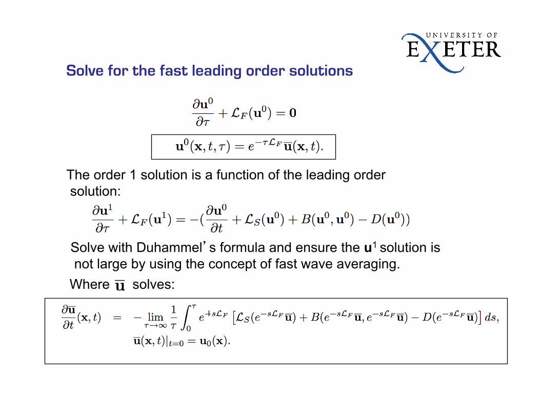
Solve for the fast leading order solutions

Solve with Duhammel’s formula and ensure the u1 solution is not large by using the concept of fast wave averaging.

The order 1 solution is a function of the leading order solution:

Where solves:

Boussinesq equations - nonlocal form in a Hilbert Space

Hilbert Space X of vector fields u in L that are divergence free and equipped with the L norm.

2

2