best available retrofit technology modeling … · best available retrofit technology modeling...
TRANSCRIPT

10333 Richmond Avenue, Suite 910, Houston TX 77042 Tel: 713.470.6546
Best Available Retrofit Technology Modeling Analysis
Huntsman Polymers Corporation
Odessa Plant TCEQ Account EB0057B
Prepared for:
Huntsman Polymers Corporation Odessa, Texas
Prepared by:
Steven H. Ramsey, P.E., BCEE Christopher J. Colville, EIT, EPI
ENVIRON International Corporation
June 2007 Project No. 26-18166A
BART Modeling -i- E N V I R O N Huntsman Odessa Plant
C O N T E N T S
Page
TEXAS PROFESSIONAL ENGINEER’S STATEMENT .............................................................1
1. INTRODUCTION ......................................................................................................................2
1.1 Purpose.............................................................................................................................2
1.2 Background information ..................................................................................................2
1.3 Potentially Affected Sources ...........................................................................................2
1.4 Exemptions ......................................................................................................................3 1.4.1 Exempt by Rule ........................................................................................................3 1.4.2 EGU Exemption .......................................................................................................4 1.4.3 TCEQ Screening Exemption Modeling....................................................................4 1.4.4 Source-Specific Exemption Modeling ......................................................................5
2. CALPUFF MODELING APPROACH ......................................................................................7
2.1 Overview..........................................................................................................................7
2.2 Class I Areas to Assess ....................................................................................................7
2.3 Air Quality Model and Inputs ..........................................................................................8 2.3.1 Modeling Domains...................................................................................................8 2.3.2 CALPUFF System Implementation..........................................................................8 2.3.3 Meteorological Data Modeling (CALMET) ............................................................9 2.3.4 Source Parameters...................................................................................................9 2.3.5 Emission Rates .......................................................................................................10 2.3.6 Dispersion Model (CALPUFF)..............................................................................12 2.3.7 Post-Processing (CALPOST).................................................................................13 2.3.8 Model Code Recompilation ...................................................................................14
3. CALPUFF MODELING RESULTS ........................................................................................15
BART Modeling -ii- E N V I R O N Huntsman Odessa Plant
T A B L E S
Page Table 2-1. CALPUFF Modeling Components ................................................................................ 9
Table 2-2. Source Parameters Used in CALPUFF Modeling Analysis......................................... 10
Table 2-3. Species Included in BART Screening Modeling Analysis .......................................... 11
Table 2-4. Emission Rates Used in CALPUFF Modeling Analysis.............................................. 11
Table 2-5. Ozone Monitoring Stations .......................................................................................... 12
Table 3-1. CALPUFF Modeling Results....................................................................................... 15
F I G U R E S
Page Figure 2-1. CENRAP South Domain................................................................................................ 7
Figure 3.1. CALPUFF Modeling Results: Class I Areas Bandelier through La Garita ................. 16
Figure 3.2. CALPUFF Modeling Results: Class I Areas Mesa Verde through Wichita Mountains .................................................................................................................... 16
A T T A C H M E N T S
Attachment A TCEQ BART Modeling Protocol
Attachment B 30 TAC Chapter 116, Subchapter M: Best Available Retrofit Technology
Attachment C CALPUFF Control File Inputs
Attachment D POSTUTIL Control File Inputs
Attachment E CALPOST Control File Inputs
Attachment F Modeling Archive

BART Modeling -1- E N V I R O N Huntsman Odessa Plant
TEXAS PROFESSIONAL ENGINEER’S STATEMENT
30 TAC 116.1510(b) requires that modeling demonstrations used to show that a BART-eligible source does not contribute to visibility impairment at any Class I area must be submitted under seal of a Texas licensed professional engineer to the Texas Commission on Environmental Quality Air Permits Division. By this statement, I hereby certify that the dispersion modeling analysis described and documented within this report was performed by me or under my direct supervision and that the model inputs used and results presented are true and correct to the best of my knowledge. Any limitations with respect to sources or availability of information and assumptions used in the analysis are noted within the report.
Steven Hunter Ramsey, P.E. Date
Texas Licensed Professional Engineer Number 69070

BART Modeling -2- E N V I R O N Huntsman Odessa Plant
1. INTRODUCTION
1.1 Purpose
The Huntsman Polymers Corporation (Huntsman) retained ENVIRON International Corporation (ENVIRON) to perform a source-specific Best Available Retrofit Technology (BART) modeling analysis using the CALPUFF model for the Huntsman Odessa Plant located near Odessa, Texas. The source-specific BART screening modeling analysis presented within this report follows Texas Commission on Environmental Quality (TCEQ) and Central States Regional Air Planning Association (CENRAP) guidance.1,2 TCEQ guidance is included as Attachment A to this report.
1.2 Background information
In 1999, the EPA promulgated rules to address visibility impairment – often referred to as “regional haze” – at designated federal Class I areas. These include areas such as national parks and wilderness areas where visibility is considered to be an important part of the visitor experience.3 There are two Class I areas in Texas – Big Bend and Guadalupe National Parks – as well as a number in surrounding states in close proximity to Texas. Guidelines providing direction to the states for implementing the regional haze rules were issued by EPA in July 2005. Affected states, including Texas, are required to develop plans for addressing visibility impairment. This includes a requirement that certain existing sources be equipped with Best Available Retrofit Technology, or BART. Texas is required to submit a regional haze plan to EPA no later than December 17, 2007.
1.3 Potentially Affected Sources
The Texas Commission on Environmental Quality (TCEQ) regional haze rule adopted on January 10, 2007 (presented in Attachment B), identifies potentially affected sources as those:4
• Belonging to one of 26 industry source categories;5
1 Best Available Retrofit Technology (BART) Modeling Protocol to Determine Sources Subject to BART in the State of Texas, January 2007, prepared by the TCEQ. 2 Alpine Geophysics, LLC.2005. CENRAP BART Modeling Guidelines. 3 40 CFR 51, Subpart P 4 30 TAC Chapter 116, Subchapter M, effective February 7, 2007. 5 (1) fossil fuel-fired steam electric plants of more than 250 MMBtu/hour heat input; (2) coal-cleaning plants (thermal dryers); (3) Kraft pulp mills; (4) Portland cement plants; (5) primary zinc smelters; (6) iron and steel mill plants; (7) primary aluminum ore reduction plants; (8) primary copper smelters; (9) municipal incinerators capable of charging more than 250 tons of refuse per day; (10) hydrofluoric, sulfuric, and nitric acid plants; (11) petroleum refineries; (12) lime plants; (13) phosphate rock processing plants; (14) coke oven batteries; (15) sulfur recovery plants; (16) carbon black plants (furnace process); (17) primary lead smelters; (18) fuel conversion plants; (19) sintering plants; (20) secondary metal production facilities; (21) chemical process plants; (22) fossil fuel-fired boilers of more than 250 MMBtu/hour heat input; (23) petroleum storage and transfer facilities with capacity exceeding 300,000 barrels; (24) taconite ore processing facilities; (25) glass fiber processing plants; and (26) charcoal production facilities.
BART Modeling -3- E N V I R O N Huntsman Odessa Plant
• Having the potential to emit (PTE) 250 tons per year or more of any visibility-impairing pollutant;6 and
• Not in operation prior to August 7, 1962, and in existence on August 7, 1977.
Based on results of a survey completed by potential BART-eligible sources and submitted to the TCEQ in 2005, 126 accounts were identified as potentially BART-eligible. This includes the Huntsman Odessa Plant.
1.4 Exemptions
In 30 TAC 116.1510, the regulations identify four methods of exempting a BART-eligible source from the engineering analysis (described in 30 TAC 116.1520) and control requirements (described in 30 TAC 116.1530) of BART. These exemptions are as follows:
• Exempt by rule based on potential emissions and distance to the nearest Class I area.
• Electric Generating units (EGUs) participating in the Clean Air Interstate Rule (for nitrogen oxides and sulfur dioxide only).
• Screening exemption modeling conducted by the TCEQ.
• Source-specific exemption modeling.
Following is a brief discussion of each exemption.
1.4.1 Exempt by Rule
Following EPA guidance, the TCEQ has established exemptions based on potential emissions and distance to the nearest Class I area.
• Sources with the potential-to-emit (PTE) less than 500 tons per year of combined nitrogen oxides (NOX) and sulfur dioxide (SO2) and located more than 50 kilometers (km) from any Class I area are not subject to BART for NOX and SO2.
• Sources with the PTE less than 1,000 tons per year of combined NOX and SO2 and located more than 100 km from any Class I area are not subject to BART for NOX and SO2.
• Sources with the PTE of less than 40 tons per year of NOX or SO2 are not subject to BART for that pollutant, regardless of distance to a Class I area.
• Sources with the PTE less than 15 tons per year of particulate matter less than 10 microns in diameter (PM10) are not subject to BART for PM10, regardless of distance to a Class I area.
PTE is defined in 30 TAC 116.10 (27) as “The maximum capacity of a stationary source to emit a pollutant under its physical and operational design. Any physical or enforceable operational limitation on the capacity of the stationary source to emit a pollutant, including air pollution control equipment and restrictions on hours of operation or on the type or amount of material combusted, stored, or processed, may be treated as part of its 6 Visibility-impairing air pollutant is defined in 30 TAC 116.1500(2) as “Any of the following: nitrogen oxides, sulfur dioxide, or particulate matter.”
BART Modeling -4- E N V I R O N Huntsman Odessa Plant
design only if the limitation or the effect it would have on emissions is federally enforceable.” To take advantage of a model plant exemption, the PTE must be federally enforceable no later than April 30, 2007.
PTE for BART-eligible emission units at the Huntsman Odessa Plant is less than 1,000 tons per year and the distance to the closest Class I area is greater than 100 km. Therefore, the source is not subject to BART for NOX and SO2. Emissions of PM10, however, are greater than the 15 ton per year threshold. Therefore, the Odessa Plant is not exempt by rule from BART for particulate matter.
1.4.2 EGU Exemption
BART-eligible EGUs that participate in the Clean Air Interstate Rule trading program for NOX and SO2 are not subject to the engineering analysis and control requirements of BART. The Huntsman Odessa Plant is not an EGU and does not qualify for this exemption.
1.4.3 TCEQ Screening Exemption Modeling
The TCEQ performed cumulative group BART screening exemption modeling using the Comprehensive Air Quality Model with extensions (CAMx). The 126 potentially BART-eligible sources were included in the screening exemption modeling.
Three types of BART screening exemption modeling were conducted:
• BART sources volatile organic compound (VOC) zero-out modeling to ascertain whether or not Texas BART VOC emissions cause or contribute to visibility impairment at any Class I area;
• BART sources primary particulate matter (PM) zero-out and chemically inert modeling to ascertain whether or not BART primary PM emissions cause or contribute to visibility impairment at any Class I area; and
• BART sources SO2 and NOX modeling using the PM Source Apportionment Technology (PSAT) and the Plume-in-Grid (PiG) subgrid-scale point source model.
Findings were as follows:
• The VOC zero-out modeling analysis indicated that visibility impacts at Class I areas due to VOC emissions from all Texas BART sources were well below the 0.5 deciview (dv) significance threshold.7 As a result of this finding, the TCEQ decided to exclude VOC from the definition of visibility-impairing pollutant.
• Visibility impacts due to PM emissions were greater than the 0.5 dv significance threshold for two EGU and one non-EGU accounts. The EGUs are TXU’s Monticello Steam Electric Station and AEP’s Welsh Power Plant. The non-EGU is International Paper’s Texarkana Mill.
• Visibility impacts due to SO2 and NOX emissions were greater than the 0.5 dv significance threshold for
7 A deciview is a measure of visibility impairment.
BART Modeling -5- E N V I R O N Huntsman Odessa Plant
source groupings that included 48 accounts.
For a more detailed description of the BART screening exemption modeling and the results of the modeling, the reader is referred to the following documents:
• Final Report, Screening Analysis of Potential BART-Eligible Sources in Texas, September 27, 2006, prepared by ENVIRON International Corporation;8 and
• ADDENDUM I, BART Exemption Screening Analysis, DRAFT, December 6, 2006, prepared by ENVIRON International Corporation.9
30 TAC 116.1510(e) specifies that:
“Any BART-eligible source that has been screened out by the Texas Commission on Environmental Quality-conducted screening modeling is not subject to the requirements of [BART] if the owner or operator has reviewed that modeling inputs for that source and the executive director receives written certification that the inputs are correct no later than February 28, 2007.”
The Huntsman Odessa Plant passed the screening analysis for PM, NOX and SO2. However, certain PM emissions (specifically, emissions from a cooling tower) were not included in the TCEQ’s screening analysis. As a result, Huntsman could not certify that the emissions used in the screening analysis were an accurate representation of worst-case actual 24-hour emissions. No model plant was developed by the TCEQ for the Class I Area closest to the Huntsman Odessa Plant: Carlsbad Caverns National Park in New Mexico. Therefore, the model plant approach is not available for demonstrating insignificant impacts and exemption from BART.
1.4.4 Source-Specific Exemption Modeling
TCEQ regulations state that:
“The owner or operator of a BART-eligible source may demonstrate, using a model and modeling guidelines approved by the executive director, that the source does not contribute to visibility impairment at a Class I area. A BART-eligible source that does not contribute to visibility impairment at any Class I area is not subject to the requirements of [BART]. A source is considered to not contribute to visibility impairment if, as demonstrated by modeling performed by the executive director or performed in accordance with the guidelines approved by the executive director, it causes a visibility impairment of less than 0.5 deciviews at all Class I areas.”
Exemption modeling is to be submitted to the TCEQ under the seal of a Texas professional engineer.
8 http://www.tceq.state.tx.us/assets/public/implementation/air/sip/bart/BART_FinalReport.pdf. 9 http://www.tceq.state.tx.us/assets/public/implementation/air/sip/bart/addendum-screening.pdf.

BART Modeling -6- E N V I R O N Huntsman Odessa Plant
TCEQ guidance identifies the following exemption modeling options for potentially BART-affected sources:
• CALPUFF for Class I areas located within 300 km of the source;
• CALPUFF for Class I areas located beyond 300 km of the source for a conservative screening analysis; and
• CAMx for Class I areas located beyond 300 km of the source in a refined analysis.
The Huntsman Odessa Plant is located approximately 190 km from the nearest Class I area: Carlsbad Caverns National Park in New Mexico.
BART Modeling -7- E N V I R O N Huntsman Odessa Plant
2. CALPUFF MODELING APPROACH
2.1 Overview
One of the air quality modeling approaches in EPA’s BART guidance is an individual source attribution approach. Specifically, this entails modeling source-specific BART-eligible units and comparing modeled impacts to the deciview threshold. The modeling approach discussed here is specifically designed for conducting a source-specific BART screening modeling analysis.
2.2 Class I Areas to Assess
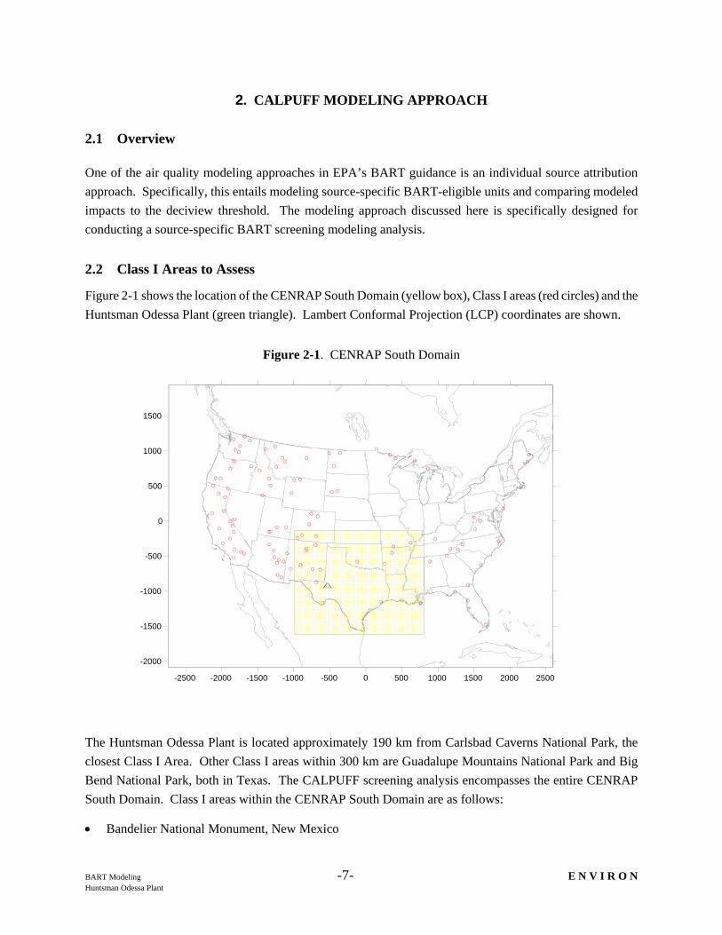
Figure 2-1 shows the location of the CENRAP South Domain (yellow box), Class I areas (red circles) and the Huntsman Odessa Plant (green triangle). Lambert Conformal Projection (LCP) coordinates are shown.
Figure 2-1. CENRAP South Domain
The Huntsman Odessa Plant is located approximately 190 km from Carlsbad Caverns National Park, the closest Class I Area. Other Class I areas within 300 km are Guadalupe Mountains National Park and Big Bend National Park, both in Texas. The CALPUFF screening analysis encompasses the entire CENRAP South Domain. Class I areas within the CENRAP South Domain are as follows:
• Bandelier National Monument, New Mexico
-2500 -2000 -1500 -1000 -500 0 500 1000 1500 2000 2500 -2000
-1500
-1000
-500
0
500
1000
1500

BART Modeling -8- E N V I R O N Huntsman Odessa Plant
• Big Bend National Park, Texas
• Bosque del Apache National Wildlife Refuge, New Mexico
• Breton Wilderness Area, Louisiana
• Caney Creek Wilderness Area, Arkansas
• Carlsbad Caverns National Park, New Mexico
• Great Sand Dunes Wilderness Area, Colorado
• Guadalupe Mountains National Park, Texas
• Hercules-Glade Wilderness Area, Missouri
• La Garita Wilderness Area, Colorado
• Mesa Verde National Park, Colorado
• Mingo Wilderness Area, Missouri
• Pecos Wilderness Area, New Mexico
• Salt Creek Wilderness Area, New Mexico
• San Pedro Parks Wilderness Area, New Mexico
• Upper Buffalo Wilderness Area, Arkansas
• Weminuche Wilderness Area, Colorado
• Wheeler Peak Wilderness Area, New Mexico
• White Mountain Wilderness Area, New Mexico
• Wichita Mountains National Wildlife Refuge, Oklahoma
2.3 Air Quality Model and Inputs
2.3.1 Modeling Domains
The CALPUFF source-specific screening modeling for the Huntsman Odessa Plant is conducted with the CENRAP South Domain 6 km grid as shown in Figure 2-1. The domain extents are as follows.
• SW Corner (1,1): -1008.0 km, -1620.0 km
• NX, NY: 306, 246
• DX, DY: 6 km 6 km
2.3.2 CALPUFF System Implementation
There are three main components to the CALPUFF model:
• Meteorological Data Modeling (CALMET);
BART Modeling -9- E N V I R O N Huntsman Odessa Plant
• Dispersion Modeling (CALPUFF); and
• Post-processing (POSTUTIL / CALPOST).
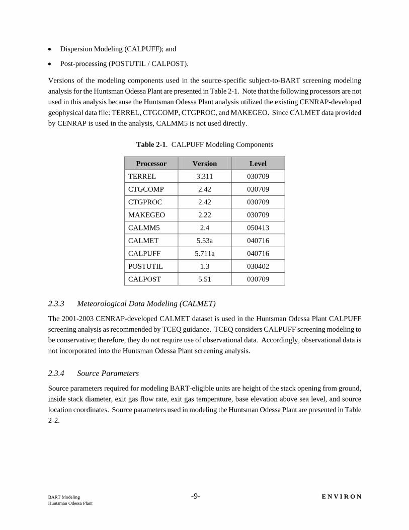
Versions of the modeling components used in the source-specific subject-to-BART screening modeling analysis for the Huntsman Odessa Plant are presented in Table 2-1. Note that the following processors are not used in this analysis because the Huntsman Odessa Plant analysis utilized the existing CENRAP-developed geophysical data file: TERREL, CTGCOMP, CTGPROC, and MAKEGEO. Since CALMET data provided by CENRAP is used in the analysis, CALMM5 is not used directly.
Table 2-1. CALPUFF Modeling Components
Processor Version Level
TERREL 3.311 030709
CTGCOMP 2.42 030709
CTGPROC 2.42 030709
MAKEGEO 2.22 030709
CALMM5 2.4 050413
CALMET 5.53a 040716
CALPUFF 5.711a 040716
POSTUTIL 1.3 030402
CALPOST 5.51 030709
2.3.3 Meteorological Data Modeling (CALMET)
The 2001-2003 CENRAP-developed CALMET dataset is used in the Huntsman Odessa Plant CALPUFF screening analysis as recommended by TCEQ guidance. TCEQ considers CALPUFF screening modeling to be conservative; therefore, they do not require use of observational data. Accordingly, observational data is not incorporated into the Huntsman Odessa Plant screening analysis.
2.3.4 Source Parameters
Source parameters required for modeling BART-eligible units are height of the stack opening from ground, inside stack diameter, exit gas flow rate, exit gas temperature, base elevation above sea level, and source location coordinates. Source parameters used in modeling the Huntsman Odessa Plant are presented in Table 2-2.
BART Modeling -10- E N V I R O N Huntsman Odessa Plant
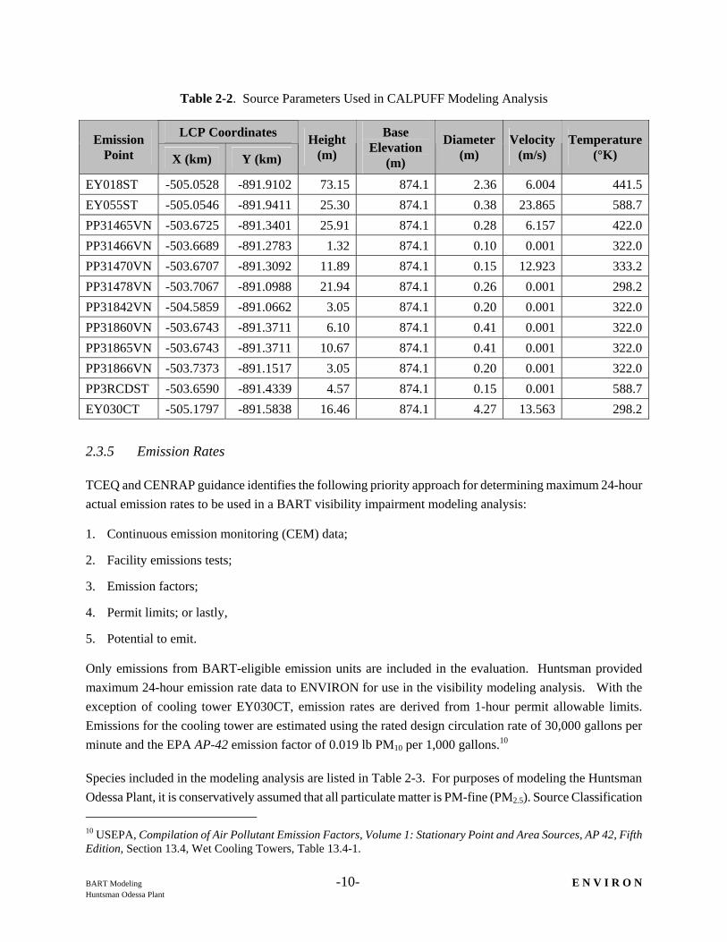
Table 2-2. Source Parameters Used in CALPUFF Modeling Analysis
LCP Coordinates Emission Point X (km) Y (km)
Height (m)
Base Elevation
(m)
Diameter (m)
Velocity (m/s)
Temperature (°K)
EY018ST -505.0528 -891.9102 73.15 874.1 2.36 6.004 441.5EY055ST -505.0546 -891.9411 25.30 874.1 0.38 23.865 588.7PP31465VN -503.6725 -891.3401 25.91 874.1 0.28 6.157 422.0PP31466VN -503.6689 -891.2783 1.32 874.1 0.10 0.001 322.0PP31470VN -503.6707 -891.3092 11.89 874.1 0.15 12.923 333.2PP31478VN -503.7067 -891.0988 21.94 874.1 0.26 0.001 298.2PP31842VN -504.5859 -891.0662 3.05 874.1 0.20 0.001 322.0PP31860VN -503.6743 -891.3711 6.10 874.1 0.41 0.001 322.0PP31865VN -503.6743 -891.3711 10.67 874.1 0.41 0.001 322.0PP31866VN -503.7373 -891.1517 3.05 874.1 0.20 0.001 322.0PP3RCDST -503.6590 -891.4339 4.57 874.1 0.15 0.001 588.7EY030CT -505.1797 -891.5838 16.46 874.1 4.27 13.563 298.2
2.3.5 Emission Rates
TCEQ and CENRAP guidance identifies the following priority approach for determining maximum 24-hour actual emission rates to be used in a BART visibility impairment modeling analysis:
1. Continuous emission monitoring (CEM) data;
2. Facility emissions tests;
3. Emission factors;
4. Permit limits; or lastly,
5. Potential to emit.
Only emissions from BART-eligible emission units are included in the evaluation. Huntsman provided maximum 24-hour emission rate data to ENVIRON for use in the visibility modeling analysis. With the exception of cooling tower EY030CT, emission rates are derived from 1-hour permit allowable limits. Emissions for the cooling tower are estimated using the rated design circulation rate of 30,000 gallons per minute and the EPA AP-42 emission factor of 0.019 lb PM10 per 1,000 gallons.10
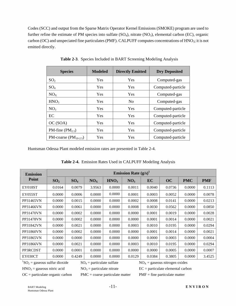
Species included in the modeling analysis are listed in Table 2-3. For purposes of modeling the Huntsman Odessa Plant, it is conservatively assumed that all particulate matter is PM-fine (PM2.5). Source Classification 10 USEPA, Compilation of Air Pollutant Emission Factors, Volume 1: Stationary Point and Area Sources, AP 42, Fifth Edition, Section 13.4, Wet Cooling Towers, Table 13.4-1.
BART Modeling -11- E N V I R O N Huntsman Odessa Plant
Codes (SCC) and output from the Sparse Matrix Operator Kernel Emissions (SMOKE) program are used to further refine the estimate of PM species into sulfate (SO4), nitrate (NO3), elemental carbon (EC), organic carbon (OC) and unspeciated fine particulates (PMF). CALPUFF computes concentrations of HNO3; it is not emitted directly.
Table 2-3. Species Included in BART Screening Modeling Analysis
Species Modeled Directly Emitted Dry Deposited
SO2 Yes Yes Computed-gas
SO4 Yes Yes Computed-particle
NOX Yes Yes Computed-gas
HNO3 Yes No Computed-gas
NO3 Yes Yes Computed-particle
EC Yes Yes Computed-particle
OC (SOA) Yes Yes Computed-particle
PM-fine (PM2.5) Yes Yes Computed-particle
PM-coarse (PM10-2.5) Yes Yes Computed-particle
Huntsman Odessa Plant modeled emission rates are presented in Table 2-4.
Table 2-4. Emission Rates Used in CALPUFF Modeling Analysis
Emission Rate (g/s)1 Emission Point SO2 SO4 NOX HNO3 NO3 EC OC PMC PMF
EY018ST 0.0164 0.0079 3.9563 0.0000 0.0011 0.0040 0.0736 0.0000 0.1113
EY055ST 0.0000 0.0006 0.0000 0.0000 0.0001 0.0003 0.0052 0.0000 0.0078 PP31465VN 0.0000 0.0015 0.0000 0.0000 0.0002 0.0008 0.0141 0.0000 0.0213 PP31466VN 0.0000 0.0061 0.0000 0.0000 0.0008 0.0030 0.0562 0.0000 0.0850 PP31470VN 0.0000 0.0002 0.0000 0.0000 0.0000 0.0001 0.0019 0.0000 0.0028 PP31478VN 0.0000 0.0002 0.0000 0.0000 0.0000 0.0001 0.0014 0.0000 0.0021 PP31842VN 0.0000 0.0021 0.0000 0.0000 0.0003 0.0010 0.0195 0.0000 0.0294 PP31860VN 0.0000 0.0002 0.0000 0.0000 0.0000 0.0001 0.0014 0.0000 0.0021 PP31865VN 0.0000 0.0000 0.0000 0.0000 0.0000 0.0000 0.0003 0.0000 0.0004 PP31866VN 0.0000 0.0021 0.0000 0.0000 0.0003 0.0010 0.0195 0.0000 0.0294 PP3RCDST 0.0000 0.0001 0.0000 0.0000 0.0000 0.0000 0.0005 0.0000 0.0007 EY030CT 0.0000 0.4249 0.0000 0.0000 0.0129 0.0384 0.3805 0.0000 3.4525 1SO2 = gaseous sulfur dioxide SO4 = particulate sulfate NOX = gaseous nitrogen oxides HNO3 = gaseous nitric acid NO3 = particulate nitrate EC = particulate elemental carbon OC = particulate organic carbon PMC = coarse particulate matter PMF = fine particulate matter
BART Modeling -12- E N V I R O N Huntsman Odessa Plant
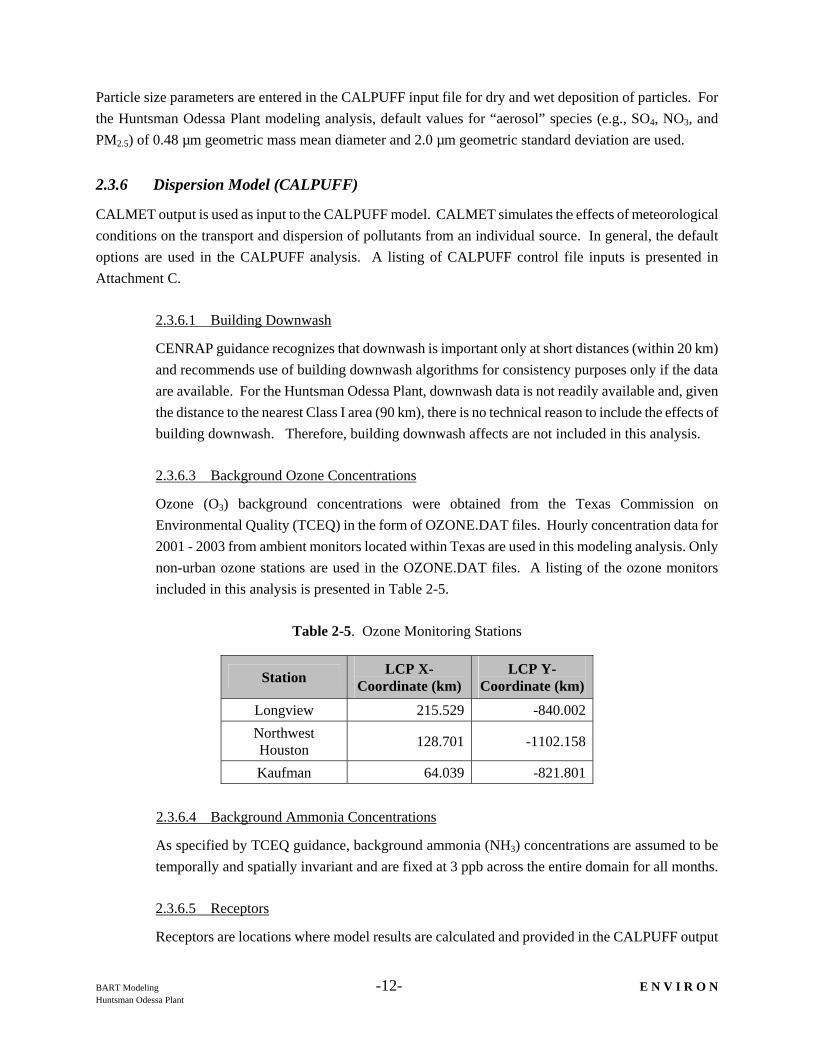
Particle size parameters are entered in the CALPUFF input file for dry and wet deposition of particles. For the Huntsman Odessa Plant modeling analysis, default values for “aerosol” species (e.g., SO4, NO3, and PM2.5) of 0.48 µm geometric mass mean diameter and 2.0 µm geometric standard deviation are used.
2.3.6 Dispersion Model (CALPUFF)
CALMET output is used as input to the CALPUFF model. CALMET simulates the effects of meteorological conditions on the transport and dispersion of pollutants from an individual source. In general, the default options are used in the CALPUFF analysis. A listing of CALPUFF control file inputs is presented in Attachment C.
2.3.6.1 Building Downwash
CENRAP guidance recognizes that downwash is important only at short distances (within 20 km) and recommends use of building downwash algorithms for consistency purposes only if the data are available. For the Huntsman Odessa Plant, downwash data is not readily available and, given the distance to the nearest Class I area (90 km), there is no technical reason to include the effects of building downwash. Therefore, building downwash affects are not included in this analysis.
2.3.6.3 Background Ozone Concentrations
Ozone (O3) background concentrations were obtained from the Texas Commission on Environmental Quality (TCEQ) in the form of OZONE.DAT files. Hourly concentration data for 2001 - 2003 from ambient monitors located within Texas are used in this modeling analysis. Only non-urban ozone stations are used in the OZONE.DAT files. A listing of the ozone monitors included in this analysis is presented in Table 2-5.
Table 2-5. Ozone Monitoring Stations
Station LCP X-Coordinate (km)
LCP Y-Coordinate (km)
Longview 215.529 -840.002 Northwest Houston 128.701 -1102.158
Kaufman 64.039 -821.801
2.3.6.4 Background Ammonia Concentrations
As specified by TCEQ guidance, background ammonia (NH3) concentrations are assumed to be temporally and spatially invariant and are fixed at 3 ppb across the entire domain for all months.
2.3.6.5 Receptors
Receptors are locations where model results are calculated and provided in the CALPUFF output
BART Modeling -13- E N V I R O N Huntsman Odessa Plant
files. Receptor locations are derived from the National Park Service (NPS) Class I area receptor database.11 The receptors are kept at the one (1) km spacing provided by the NPS.
2.3.6.6 Model Output
CALPUFF modeling results are displayed in units of micrograms per cubic meter (µg/m3). CALPUFF output files are post-processed using CALPOST to determine visibility impacts in deciviews.
2.3.7 Post-Processing (CALPOST)
Hourly concentration outputs from CALPUFF are processed using POSTUTIL and CALPOST to determine impacts on visibility. POSTUTIL takes the concentration file output from CALPUFF and recalculates the nitric acid and nitrate partition based on total available sulfate and ammonia. CALPOST uses the concentration file processed through POSTUTIL, along with relative humidity data, to perform visibility calculations. POSTUTIL and CALPOST control file inputs are listed in Attachments D and E, respectively.
Light extinction must be determined in order to calculate visibility. CALPOST has seven methods for computing light extinction. The Huntsman Odessa Plant analysis uses Method 6, which computes extinction from speciated particulate matter with monthly Class I area-specific relative humidity adjustment factors. Relative humidity correction factors [f(RH)s] are applied to sulfate and nitrate concentration outputs from CALPUFF. Relative humidity correction factors are obtained from EPA’s “Guidance for Estimating Natural Visibility Conditions under the Regional Haze Rule.”12 The PM2.5 concentrations are considered part of the dry light extinction equation and do not have a humidity adjustment factor. The light extinction equation is the sum of the wet sulfate and nitrate and dry components (PM2.5 plus Rayleigh scattering) which is 10 inverse megameters (Mm-1).
Perceived visibility in deciviews is derived from the light extinction coefficient. The visibility change related to background is calculated using the modeled and established natural visibility conditions. For the Huntsman Odessa Plant evaluation, daily visibility is expressed as a change in deciviews compared to natural visibility conditions. Natural visibility conditions are based on the annual average natural levels of aerosol components at each Class I area taken from the EPA’s “Guidance for Estimating Natural Visibility Conditions Under the Regional Haze Rule.”13
To determine whether or not a source may significantly contribute to visibility impairment at a Class I area, in a cooperative agreement with the FLMs and EPA Region VI and VII, CENRAP guidance deviates from use of 98th percentile impacts. The CALMET datasets, as described in the TCEQ protocol, were processed without use of surface and upper air observations in the CALMET wind field interpolation. In some applications, this may lead to potentially less conservatism in the CALPUFF visibility results compared with the use of CALMET with observations. As a result CENRAP agreed to EPA’s recommendation that the
11 http://www2.nature.nps.gov/air/maps/receptors/index.cfm. 12 U.S. EPA (September 2003). Regional Haze: Estimating Natural Visibility Conditions Under the Regional Haze Rule. EPA-454/B-03-005. 13 Ibid.
BART Modeling -14- E N V I R O N Huntsman Odessa Plant
maximum visibility impact rather than the 98th percentile value should be used for screening analyses performed using the CENRAP-developed CALMET datasets. This approach is used in performing the Huntsman Odessa Plant screening analysis.
2.3.8 Model Code Recompilation
To ensure compatibility with the CENRAP-developed CALMET files, CALPUFF, POSTUTIL and CALPOST model codes were recompiled using the Lahey-Fujitsu FORTRAN Express v7.1 compiler after making changes to the respective parameter files as follows (new parameter value provided).14
• CALPUFF (modified params.puf):
− MXNX = 306
− MXNXG = 306
− MXSS = 375 (not applicable to this screening analysis)
− MXPUFF = 100500 (not applicable to this screening analysis)
• POSTUTIL (modified params.utl):
− MXGX = 306
− MXGY = 246
− MXSS = 375 (not applicable to this screening analysis)
− MXPS = 375 (not applicable to this screening analysis)
• CALPOST (modified params.pst):
− MXGX = 306
− MXGY = 246
− MXSS = 375 (not applicable to this screening analysis)
Updated executables for each program were created using the Lahey-Fujitsu FORTRAN Express v7.1 compiler following changes to the parameter files. These updated executables were used in this CALPUFF analysis. The updated parameter files are included in the electronic archive submitted with this modeling analysis.
14 CALPUFF, POSTUTIL, and CALPOST have been modified for use in other BART modeling investigations, including those conducted in a refined mode. The same executables have been used for all facilities. As a result, some parameter changes are not applicable to a screening analysis and are noted accordingly.
BART Modeling -15- E N V I R O N Huntsman Odessa Plant
3. CALPUFF MODELING RESULTS
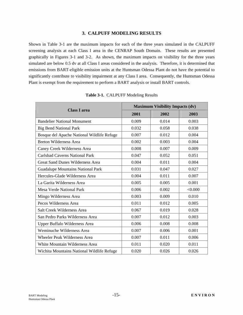
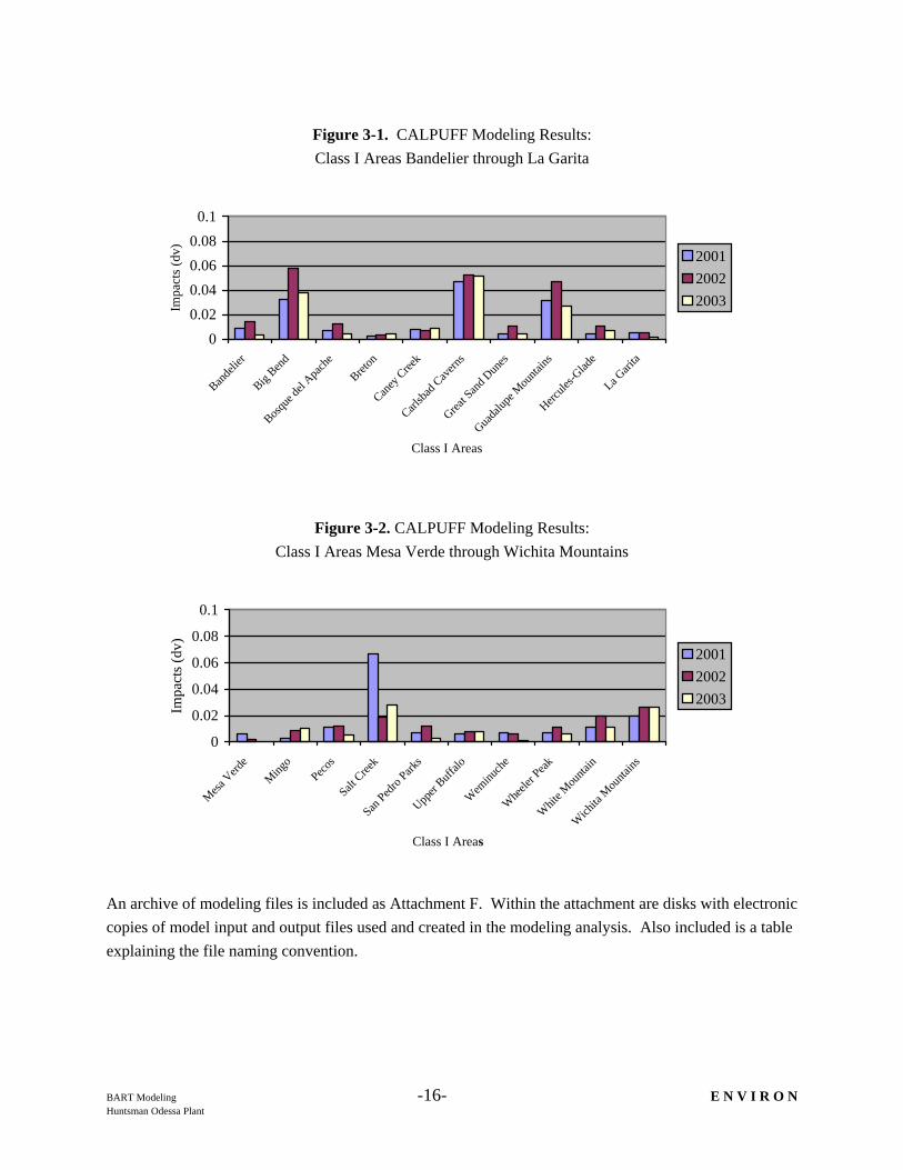
Shown in Table 3-1 are the maximum impacts for each of the three years simulated in the CALPUFF screening analysis at each Class I area in the CENRAP South Domain. These results are presented graphically in Figures 3-1 and 3-2. As shown, the maximum impacts on visibility for the three years simulated are below 0.5 dv at all Class I areas considered in the analysis. Therefore, it is determined that emissions from BART-eligible emission units at the Huntsman Odessa Plant do not have the potential to significantly contribute to visibility impairment at any Class I area. Consequently, the Huntsman Odessa Plant is exempt from the requirement to perform a BART analysis or install BART controls.
Table 3-1. CALPUFF Modeling Results
Maximum Visibility Impacts (dv) Class I area
2001 2002 2003
Bandelier National Monument 0.009 0.014 0.003 Big Bend National Park 0.032 0.058 0.038 Bosque del Apache National Wildlife Refuge 0.007 0.012 0.004 Breton Wilderness Area 0.002 0.003 0.004 Caney Creek Wilderness Area 0.008 0.007 0.009 Carlsbad Caverns National Park 0.047 0.052 0.051 Great Sand Dunes Wilderness Area 0.004 0.011 0.004 Guadalupe Mountains National Park 0.031 0.047 0.027 Hercules-Glade Wilderness Area 0.004 0.011 0.007 La Garita Wilderness Area 0.005 0.005 0.001 Mesa Verde National Park 0.006 0.002 <0.000 Mingo Wilderness Area 0.003 0.009 0.010 Pecos Wilderness Area 0.011 0.012 0.005 Salt Creek Wilderness Area 0.067 0.019 0.028 San Pedro Parks Wilderness Area 0.007 0.012 0.003 Upper Buffalo Wilderness Area 0.006 0.008 0.008 Weminuche Wilderness Area 0.007 0.006 0.001 Wheeler Peak Wilderness Area 0.007 0.011 0.006 White Mountain Wilderness Area 0.011 0.020 0.011 Wichita Mountains National Wildlife Refuge 0.020 0.026 0.026
BART Modeling -16- E N V I R O N Huntsman Odessa Plant
Figure 3-1. CALPUFF Modeling Results: Class I Areas Bandelier through La Garita
Figure 3-2. CALPUFF Modeling Results: Class I Areas Mesa Verde through Wichita Mountains
An archive of modeling files is included as Attachment F. Within the attachment are disks with electronic copies of model input and output files used and created in the modeling analysis. Also included is a table explaining the file naming convention.
00.020.040.060.08
0.1
Bande
lier
Big Ben
d
Bosque
del A
pach
eBret
on
Caney
Creek
Carlsba
d Cav
erns
Great S
and D
unes
Guada
lupe M
ounta
ins
Hercule
s-Glad
e
La Gari
ta
Class I Areas
Impa
cts (
dv)
200120022003
0
0.02
0.04
0.06
0.08
0.1
Mesa V
erde
Mingo
Pecos
Salt Cree
k
San Ped
ro Park
s
Upper
Buffalo
Wem
inuch
e
Whe
eler P
eak
Whit
e Mou
ntain
Wich
ita M
ounta
ins
Class I Areas
Impa
cts (
dv)
200120022003
BART Modeling E N V I R O N Huntsman Odessa Plant
ATTACHMENT A
TCEQ BART Modeling Protocol
January 2007
Best Available Retrofit Technology (BART)
Modeling Protocol to Determine Sources Subject to BART
in the State of Texas
Air Permits Division Texas Commission on Environmental Quality
Print on Recycled paper
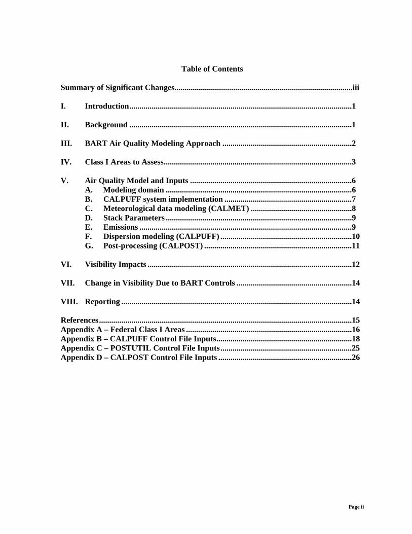
Table of Contents
Summary of Significant Changes........................................................................................iii I. Introduction..............................................................................................................1 II. Background ..............................................................................................................1 III. BART Air Quality Modeling Approach ................................................................2 IV. Class I Areas to Assess.............................................................................................3 V. Air Quality Model and Inputs ................................................................................6 A. Modeling domain ............................................................................................6 B. CALPUFF system implementation ...............................................................7 C. Meteorological data modeling (CALMET) ..................................................8 D. Stack Parameters ............................................................................................9 E. Emissions .........................................................................................................9 F. Dispersion modeling (CALPUFF) .................................................................10 G. Post-processing (CALPOST) .........................................................................11 VI. Visibility Impacts .....................................................................................................12 VII. Change in Visibility Due to BART Controls .........................................................14 VIII. Reporting ..................................................................................................................14 References.............................................................................................................................15 Appendix A – Federal Class I Areas ..................................................................................16 Appendix B – CALPUFF Control File Inputs...................................................................18 Appendix C – POSTUTIL Control File Inputs.................................................................25 Appendix D – CALPOST Control File Inputs ..................................................................26
Page ii
Summary of Significant Changes
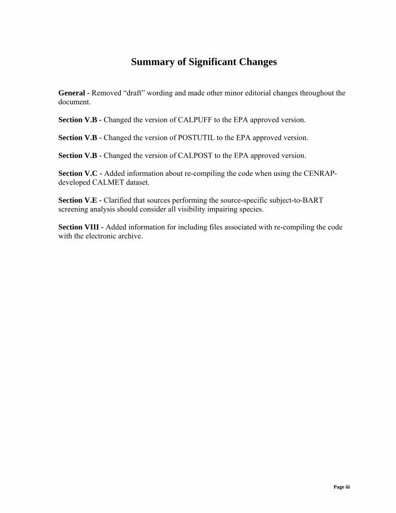
General - Removed “draft” wording and made other minor editorial changes throughout the document. Section V.B - Changed the version of CALPUFF to the EPA approved version. Section V.B - Changed the version of POSTUTIL to the EPA approved version. Section V.B - Changed the version of CALPOST to the EPA approved version. Section V.C - Added information about re-compiling the code when using the CENRAP-developed CALMET dataset. Section V.E - Clarified that sources performing the source-specific subject-to-BART screening analysis should consider all visibility impairing species. Section VIII - Added information for including files associated with re-compiling the code with the electronic archive.
Page iii

I. Introduction On July 6, 2005, the U.S. Environmental Protection Agency (EPA) published final amendments to its 1999 Regional Haze Rule in the Federal Register, including Appendix Y, the final guidance for Best Available Retrofit Technology (BART) determinations (70 FR 39104-39172). The BART rule requires the installation of BART on emission sources that fit specific criteria and “may reasonably be anticipated to cause or contribute” to visibility impairment in any Class I area. Air quality modeling is a means for determining which sources cause or contribute to visibility impairment. Texas’ proposed protocol for conducting this modeling for BART is provided herein. The Texas Commission on Environmental Quality (TCEQ) foresees two purposes for this protocol. First, sources may use the protocol to determine if BART-eligible units are subject to BART and must perform a BART analysis. Second, sources that are subject to BART will have this protocol to use as a starting point to conduct modeling required when making a BART analysis. New BART guidance, both formal and informal, continues to become available from EPA and the Federal Land Managers (FLMs) that oversee visibility in Class I areas. Texas has developed a schedule for completing BART analyses and implementing the BART strategy in order to meet State Implementation Plan (SIP) deadlines. If the state is to meet those deadlines, modeling to determine sources subject to BART and modeling to make BART analyses may need to be done before all final BART guidance from EPA and the FLMs becomes available.
II. Background Generally, Class I areas are national parks and wilderness areas in which visibility is more stringently protected under the Clean Air Act than any other areas in the United States. The Class I areas are shown in Appendix A. The BART requirements are a part of the SIP that will be submitted to EPA in late 2007. The SIP is a comprehensive plan of action to increase visibility in the Class I areas and includes reasonable progress goals in addition to the goals established by sources subject to BART.
Page 1
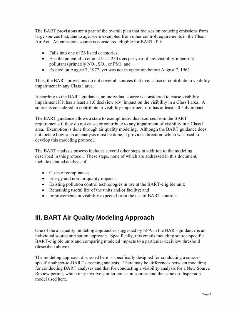
The BART provisions are a part of the overall plan that focuses on reducing emissions from large sources that, due to age, were exempted from other control requirements in the Clean Air Act. An emissions source is considered eligible for BART if it:
• Falls into one of 26 listed categories; • Has the potential to emit at least 250 tons per year of any visibility-impairing
pollutant (primarily NOx, SO2, or PM); and • Existed on August 7, 1977, yet was not in operation before August 7, 1962.
Thus, the BART provisions do not cover all sources that may cause or contribute to visibility impairment in any Class I area. According to the BART guidance, an individual source is considered to cause visibility impairment if it has a least a 1.0 deciview (dv) impact on the visibility in a Class I area. A source is considered to contribute to visibility impairment if it has at least a 0.5 dv impact. The BART guidance allows a state to exempt individual sources from the BART requirements if they do not cause or contribute to any impairment of visibility in a Class I area. Exemption is done through air quality modeling. Although the BART guidance does not dictate how such an analysis must be done, it provides direction, which was used to develop this modeling protocol. The BART analysis process includes several other steps in addition to the modeling described in this protocol. These steps, none of which are addressed in this document, include detailed analysis of:
• Costs of compliance; • Energy and non-air quality impacts; • Existing pollution control technologies in use at the BART-eligible unit; • Remaining useful life of the units and/or facility; and • Improvements in visibility expected from the use of BART controls.
III. BART Air Quality Modeling Approach One of the air quality modeling approaches suggested by EPA in the BART guidance is an individual source attribution approach. Specifically, this entails modeling source-specific BART-eligible units and comparing modeled impacts to a particular deciview threshold (described above). The modeling approach discussed here is specifically designed for conducting a source-specific subject-to-BART screening analysis. There may be differences between modeling for conducting BART analyses and that for conducting a visibility analysis for a New Source Review permit, which may involve similar emission sources and the same air dispersion model used here.
Page 2

In preparing this modeling protocol, the TCEQ consulted BART modeling protocols drafted by other organizations to maintain an appropriately consistent approach within the Central States Regional Air Planning Association (CENRAP). The three available BART modeling protocols consulted were:
1.
2.
3.
“Best Available Retrofit Technology (BART) Modeling Protocol to Determine Sources Subject to BART in the State of Minnesota,” final version March 2006; “Best Available Retrofit Technology (BART) Modeling Protocol to Determine Sources Subject to BART in the State of Kansas,” final version June 2006; “Screening Analysis of Potentially BART-Eligible Sources in Texas,” developed by ENVIRON International Corporation, December 2005.
This protocol is most similar to the Kansas and Minnesota final protocols. Texas is in EPA Region VI, and they will be reviewing Texas’ Regional Haze SIP, of which BART will be a part.
IV. Class I Areas to Assess Table 1, Class I Areas Evaluated for BART, contains the list of Class I areas to be included in the modeling analysis. The list was developed for the subject-to-BART screening evaluation conducted by ENVIRON for the TCEQ. Figure 1, Location of Class I Areas, shows the location of each Class I area to be evaluated. Sources conducting the source-specific subject-to-BART screening analysis should include all Class I areas that the ENVIRON screening evaluation showed their source group to have impacts greater than 0.5 dv on visibility.
Page 3
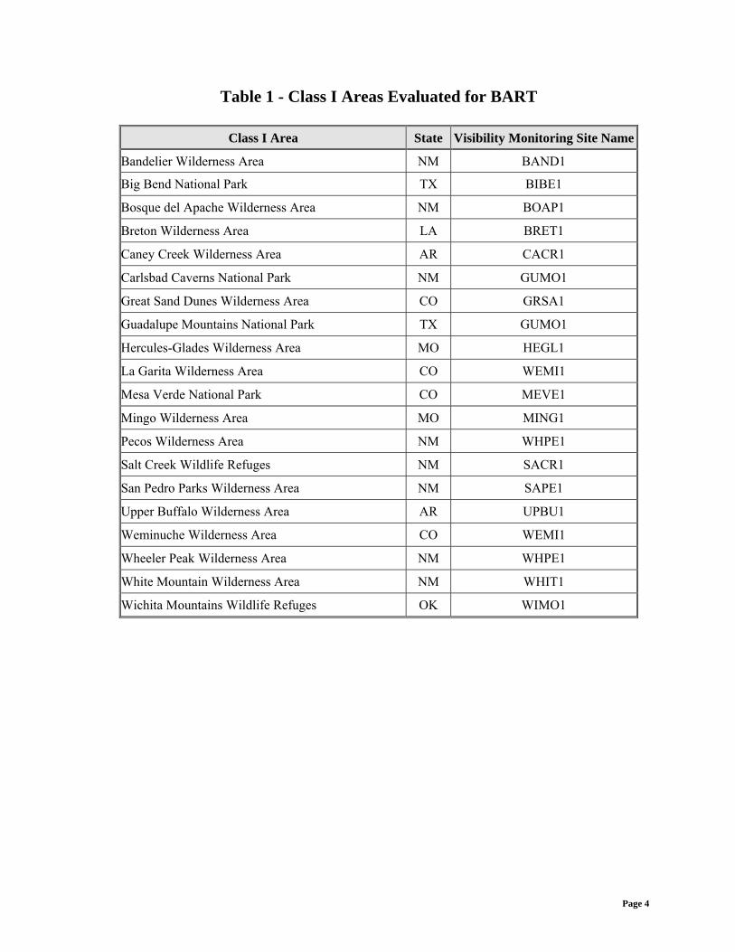
Table 1 - Class I Areas Evaluated for BART
Class I Area State Visibility Monitoring Site Name
Bandelier Wilderness Area NM BAND1
Big Bend National Park TX BIBE1
Bosque del Apache Wilderness Area NM BOAP1
Breton Wilderness Area LA BRET1
Caney Creek Wilderness Area AR CACR1
Carlsbad Caverns National Park NM GUMO1
Great Sand Dunes Wilderness Area CO GRSA1
Guadalupe Mountains National Park TX GUMO1
Hercules-Glades Wilderness Area MO HEGL1
La Garita Wilderness Area CO WEMI1
Mesa Verde National Park CO MEVE1
Mingo Wilderness Area MO MING1
Pecos Wilderness Area NM WHPE1
Salt Creek Wildlife Refuges NM SACR1
San Pedro Parks Wilderness Area NM SAPE1
Upper Buffalo Wilderness Area AR UPBU1
Weminuche Wilderness Area CO WEMI1
Wheeler Peak Wilderness Area NM WHPE1
White Mountain Wilderness Area NM WHIT1
Wichita Mountains Wildlife Refuges OK WIMO1
Page 4
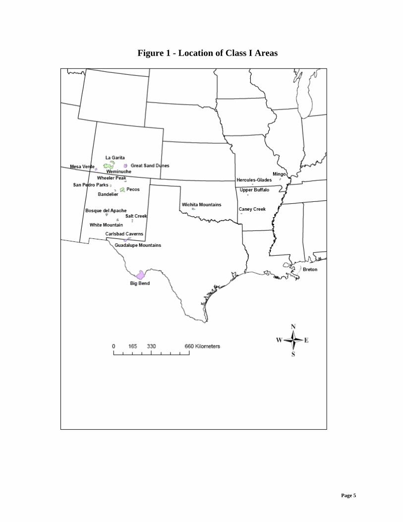
Figure 1 - Location of Class I Areas
Page 5
V. Air Quality Model and Inputs According to the final Regional Haze Rule’s BART guidance, a source “can use CALPUFF or other appropriate model to predict the visibility impacts from a single source at a Class I area.” For purposes of the source-specific subject-to-BART screening analysis, the TCEQ recommends the use of CALPUFF. The TCEQ recognizes that CALPUFF has limited ability to simulate the complex atmospheric chemistry involved in the estimation of secondary particulate formation. However, for purposes of this source-specific subject-to-BART screening analysis, the TCEQ recommends the use of CALPUFF for the following reasons:
1.
2. 3.
The increased level of effort required for conducting particulate apportionment in the regional scale, full-chemistry Eulerian model (CAMx or CMAQ) to acquire individual source contributions to Class I areas, relative to the simplicity of the CALPUFF model; The limited scope of what this modeling is to determine; and The additional modeling of BART controls that will be conducted as part of the Regional Haze SIP with the CAMx or CMAQ models.
EPA’s BART guidance recommends following the EPA’s Interagency Workgroup on Air Quality Modeling (IWAQM) guidance, Phase 2 recommendations for long-range transport. The IWAQM guidance was developed to address air quality impacts as assessed through the Prevention of Significant Deterioration (PSD) program at Class I areas, where the source generally is located beyond 50 kilometer (km) of the Class I area. The IWAQM guidance does not specifically address the type of assessment that will occur with the BART analysis. Given the uncertainties of transport and dispersion processes in CALPUFF for distances greater than 300 km, consideration may be given to the CAMx model for determining visibility impacts at Class I areas located 300 km beyond the source in a refined modeling analysis. Below is a list of options for selecting a model to use. The first two apply to the source-specific subject-to-BART screening analysis, and the third is an option for a refined modeling analysis:
1. CALPUFF for Class I areas located within 300 km of the source; 2. CALPUFF for Class I areas located beyond 300 km of the source for a conservative
screening analysis; and 3. CAMx for Class I areas located beyond 300 km of the source in a refined analysis.
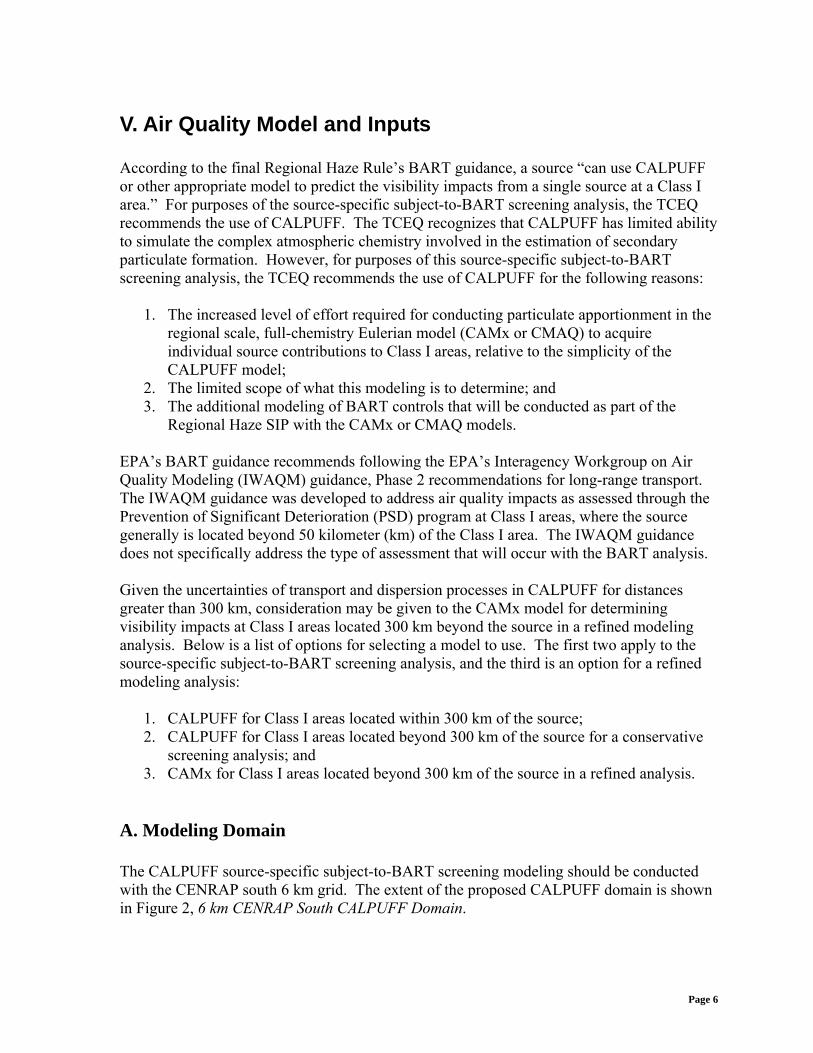
A. Modeling Domain The CALPUFF source-specific subject-to-BART screening modeling should be conducted with the CENRAP south 6 km grid. The extent of the proposed CALPUFF domain is shown in Figure 2, 6 km CENRAP South CALPUFF Domain.
Page 6
Figure 2 - 6 km CENRAP South CALPUFF Domain
CALPUFF should be applied for three annual simulations spanning the years 2001 through 2003. The IWAQM guidance allows the use of fewer than five years of meteorological data if a meteorological model using four-dimensional data assimilation is used to supply data. See the section on meteorology for more information. B. CALPUFF System Implementation There are three main components to the CALPUFF model:
1. 2. 3.
Meteorological Data Modeling (CALMET); Dispersion Modeling (CALPUFF); and Post processing (CALPOST).
Versions of the modeling components that may be used in the source-specific subject-to-BART screening analysis are shown in Table 2, CALPUFF Modeling Components.
Page 7

Table 2 - CALPUFF Modeling Components
Processor Version Level
TERREL 3.311 030709
CTGCOMP 2.42 030709
CTGPROC 2.42 030709
MAKEGEO 2.22 030709
CALMM5 2.4 050413
CALMET 5.53a 040716
CALPUFF 5.711a 040716
POSTUTIL 1.3 030402
CALPOST 5.51 030709
C. Meteorological data modeling (CALMET) The 2001-2003 CENRAP-developed CALMET dataset should be used in the source-specific subject-to-BART screening analysis. For additional information on the settings used to develop this dataset, refer to the CENRAP BART Modeling Guidelines document at www.cenrap.org/modeling_document.asp. Since no observational data were used in the CALMET outputs developed by CENRAP, the prognostic meteorological dataset from MM5 is not supplemented with surface or upper air observations during the CALMET processing. The use of observations is thought to counterbalance smoothing that may occur when using the coarse grid scale of the MM5 data. Both the EPA and FLMs commented on the draft CENRAP guidelines that observations should be used in refined CALPUFF modeling. However, the TCEQ considers this screening modeling to be conservative. Therefore, the TCEQ will not require the use of observational data. Sources may use observational data if they wish to conduct a more refined modeling analysis. In order to use the CENRAP-developed CALMET dataset, the parameter files for CALPUFF, POSTUTIL, and CALPOST may have to be edited to accommodate the size of the CENRAP-developed CALMET dataset modeling domain. Once the parameter files have been edited, the CALPUFF, POSTUTIL, and CALPOST model code will need to be re-compiled.
Page 8
D. Stack parameters Stack parameters required for modeling BART-eligible units are: height of the stack opening from ground, inside stack diameter, exit gas flow rate, exit gas temperature, base elevation above sea level, and location coordinates of the stack. Because the modeling conducted for BART is concerned with long-range transport, not localized impacts, including the effects of building downwash in the source-specific subject-to-BART screening analysis are not necessary. Sources may include the effects of building downwash if they wish to conduct a more refined modeling analysis. E. Emissions Emission rates for the BART analyses follow EPA’s BART guidance. Specifically, the 24-hour average actual emission rate with normal operations from the highest emitting day of the year should be modeled. Identification of the maximum 24-hour actual emission rates should be made for the most recent four years (2002-2005), according to the following prioritization:
1. 2. 3. 4. 5.
Continuous Emissions Monitoring (CEM) data; Facility emissions tests; Emissions factors; Permit limits; or lastly, Potential to emit.
The species that should be modeled and/or emitted in the source-specific subject-to-BART screening analysis are listed in Table 3, Species Modeled in BART Screening Analysis. Sources should include all species if the ENVIRON screening evaluation showed any of their source groups to have impacts greater than 0.5 dv on visibility.
Page 9
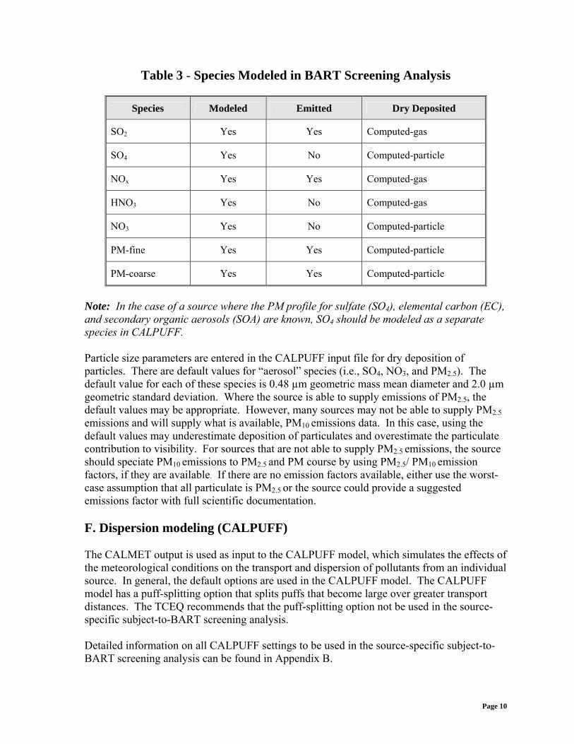
Table 3 - Species Modeled in BART Screening Analysis
Species Modeled Emitted Dry Deposited
SO2 Yes Yes Computed-gas
SO4 Yes No Computed-particle
NOx Yes Yes Computed-gas
HNO3 Yes No Computed-gas
NO3 Yes No Computed-particle
PM-fine Yes Yes Computed-particle
PM-coarse Yes Yes Computed-particle
Note: In the case of a source where the PM profile for sulfate (SO4), elemental carbon (EC), and secondary organic aerosols (SOA) are known, SO4 should be modeled as a separate species in CALPUFF. Particle size parameters are entered in the CALPUFF input file for dry deposition of particles. There are default values for “aerosol” species (i.e., SO4, NO3, and PM2.5). The default value for each of these species is 0.48 µm geometric mass mean diameter and 2.0 µm geometric standard deviation. Where the source is able to supply emissions of PM2.5, the default values may be appropriate. However, many sources may not be able to supply PM2.5
emissions and will supply what is available, PM10 emissions data. In this case, using the default values may underestimate deposition of particulates and overestimate the particulate contribution to visibility. For sources that are not able to supply PM2.5 emissions, the source should speciate PM10 emissions to PM2.5 and PM course by using PM2.5/ PM10 emission factors, if they are available. If there are no emission factors available, either use the worst-case assumption that all particulate is PM2.5 or the source could provide a suggested emissions factor with full scientific documentation. F. Dispersion modeling (CALPUFF) The CALMET output is used as input to the CALPUFF model, which simulates the effects of the meteorological conditions on the transport and dispersion of pollutants from an individual source. In general, the default options are used in the CALPUFF model. The CALPUFF model has a puff-splitting option that splits puffs that become large over greater transport distances. The TCEQ recommends that the puff-splitting option not be used in the source-specific subject-to-BART screening analysis. Detailed information on all CALPUFF settings to be used in the source-specific subject-to-BART screening analysis can be found in Appendix B.
Page 10
Ozone and ammonia concentrations: Ozone (O3) and ammonia (NH3) can be input to CALPUFF as hourly or monthly background values. Background ozone and ammonia concentrations are assumed to be temporally and spatially invariant and will be fixed at 40 and 3 ppb, respectively, across the entire domain for all months. NH3 concentrations may be derived from regional modeling outputs that CENRAP is currently developing. However, at this time these NH3 values are not available in a model ready form. Receptors: Receptors are locations where model results are calculated and provided in the CALPUFF output files. Receptor locations should be derived from the National Park Service (NPS) Class I area receptor database at www2.nature.nps.gov/air/maps/receptors/index.cfm. The discrete receptors are necessary for calculating visibility impacts in the selected Class I areas. The NPS provides receptors in all the Class I areas on a 1 km basis. These receptors should be kept at the 1 km spacing for the BART modeling. Outputs: The CALPUFF modeling results will be displayed in units of micrograms per cubic meter (µg/m3). In order to determine visibility impacts, the CALPUFF outputs must be post-processed. G. Post-processing (CALPOST) Hourly concentration outputs from CALPUFF are processed through POSTUTIL and CALPOST to determine visibility conditions. Specifically, POSTUTIL takes the concentration file output from CALPUFF and recalculates the nitric acid and nitrate partition based on total available sulfate and ammonia. CALPOST uses the concentration file processed through POSTUTIL, along with relative humidity data, to perform visibility calculations. For the source-specific subject-to-BART screening analysis, the only modeling results out of the CALPUFF modeling system of interest are the visibility impacts. Please see Appendix C and D for detailed settings for POSTUTIL and CALPOST. Light extinction: Light extinction must be computed in order to calculate visibility. CALPOST has seven methods for computing light extinction. The BART screening analysis should use Method 6, which computes extinction from speciated particulate matter with monthly Class I area-specific relative humidity adjustment factors. Relative humidity is an important factor in determining light extinction (and therefore visibility) because sulfate and nitrate aerosols, which absorb moisture from the air, have greater extinction efficiencies with greater relative humidity. The BART screening analysis should apply relative humidity correction factors (f(RH)s) to sulfate and nitrate concentration outputs from CALPUFF, which can be obtained from EPA’s “Guidance for Estimating Natural Visibility Conditions under the Regional Haze Rule (EPA, 2003). The f(RH) values for the Class I areas that should be assessed are provided in Table 4, Monthly Averaged ƒ(RH) Based on Centroid of the Class I Area.
Page 11
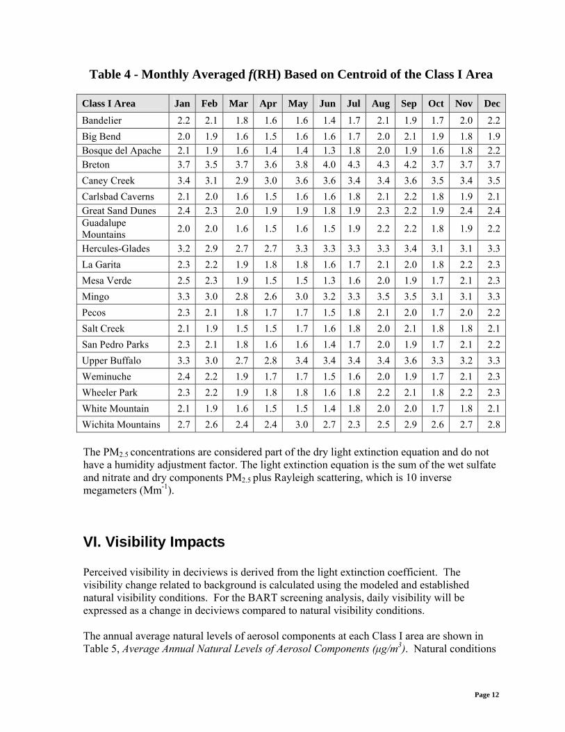
Table 4 - Monthly Averaged f(RH) Based on Centroid of the Class I Area Class I Area Jan Feb Mar Apr May Jun Jul Aug Sep Oct Nov Dec
Bandelier 2.2 2.1 1.8 1.6 1.6 1.4 1.7 2.1 1.9 1.7 2.0 2.2 Big Bend 2.0 1.9 1.6 1.5 1.6 1.6 1.7 2.0 2.1 1.9 1.8 1.9 Bosque del Apache 2.1 1.9 1.6 1.4 1.4 1.3 1.8 2.0 1.9 1.6 1.8 2.2 Breton 3.7 3.5 3.7 3.6 3.8 4.0 4.3 4.3 4.2 3.7 3.7 3.7 Caney Creek 3.4 3.1 2.9 3.0 3.6 3.6 3.4 3.4 3.6 3.5 3.4 3.5 Carlsbad Caverns 2.1 2.0 1.6 1.5 1.6 1.6 1.8 2.1 2.2 1.8 1.9 2.1 Great Sand Dunes 2.4 2.3 2.0 1.9 1.9 1.8 1.9 2.3 2.2 1.9 2.4 2.4 Guadalupe Mountains 2.0 2.0 1.6 1.5 1.6 1.5 1.9 2.2 2.2 1.8 1.9 2.2
Hercules-Glades 3.2 2.9 2.7 2.7 3.3 3.3 3.3 3.3 3.4 3.1 3.1 3.3 La Garita 2.3 2.2 1.9 1.8 1.8 1.6 1.7 2.1 2.0 1.8 2.2 2.3 Mesa Verde 2.5 2.3 1.9 1.5 1.5 1.3 1.6 2.0 1.9 1.7 2.1 2.3 Mingo 3.3 3.0 2.8 2.6 3.0 3.2 3.3 3.5 3.5 3.1 3.1 3.3 Pecos 2.3 2.1 1.8 1.7 1.7 1.5 1.8 2.1 2.0 1.7 2.0 2.2 Salt Creek 2.1 1.9 1.5 1.5 1.7 1.6 1.8 2.0 2.1 1.8 1.8 2.1 San Pedro Parks 2.3 2.1 1.8 1.6 1.6 1.4 1.7 2.0 1.9 1.7 2.1 2.2 Upper Buffalo 3.3 3.0 2.7 2.8 3.4 3.4 3.4 3.4 3.6 3.3 3.2 3.3 Weminuche 2.4 2.2 1.9 1.7 1.7 1.5 1.6 2.0 1.9 1.7 2.1 2.3 Wheeler Park 2.3 2.2 1.9 1.8 1.8 1.6 1.8 2.2 2.1 1.8 2.2 2.3 White Mountain 2.1 1.9 1.6 1.5 1.5 1.4 1.8 2.0 2.0 1.7 1.8 2.1 Wichita Mountains 2.7 2.6 2.4 2.4 3.0 2.7 2.3 2.5 2.9 2.6 2.7 2.8 The PM2.5 concentrations are considered part of the dry light extinction equation and do not have a humidity adjustment factor. The light extinction equation is the sum of the wet sulfate and nitrate and dry components PM2.5 plus Rayleigh scattering, which is 10 inverse megameters (Mm-1).
VI. Visibility Impacts Perceived visibility in deciviews is derived from the light extinction coefficient. The visibility change related to background is calculated using the modeled and established natural visibility conditions. For the BART screening analysis, daily visibility will be expressed as a change in deciviews compared to natural visibility conditions. The annual average natural levels of aerosol components at each Class I area are shown in Table 5, Average Annual Natural Levels of Aerosol Components (μg/m3). Natural conditions
Page 12
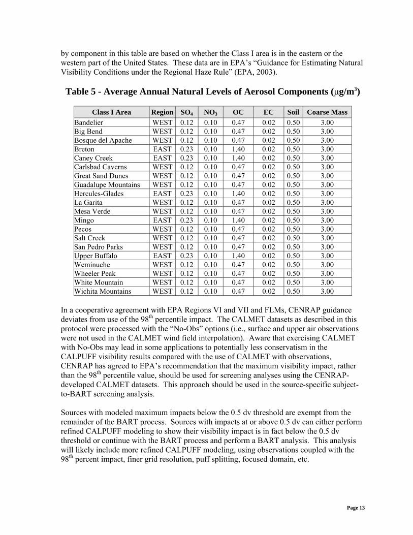
by component in this table are based on whether the Class I area is in the eastern or the western part of the United States. These data are in EPA’s “Guidance for Estimating Natural Visibility Conditions under the Regional Haze Rule” (EPA, 2003). Table 5 - Average Annual Natural Levels of Aerosol Components (μg/m3)
Class I Area Region SO4 NO3 OC EC Soil Coarse Mass
Bandelier WEST 0.12 0.10 0.47 0.02 0.50 3.00 Big Bend WEST 0.12 0.10 0.47 0.02 0.50 3.00 Bosque del Apache WEST 0.12 0.10 0.47 0.02 0.50 3.00 Breton EAST 0.23 0.10 1.40 0.02 0.50 3.00 Caney Creek EAST 0.23 0.10 1.40 0.02 0.50 3.00 Carlsbad Caverns WEST 0.12 0.10 0.47 0.02 0.50 3.00 Great Sand Dunes WEST 0.12 0.10 0.47 0.02 0.50 3.00 Guadalupe Mountains WEST 0.12 0.10 0.47 0.02 0.50 3.00 Hercules-Glades EAST 0.23 0.10 1.40 0.02 0.50 3.00 La Garita WEST 0.12 0.10 0.47 0.02 0.50 3.00 Mesa Verde WEST 0.12 0.10 0.47 0.02 0.50 3.00 Mingo EAST 0.23 0.10 1.40 0.02 0.50 3.00 Pecos WEST 0.12 0.10 0.47 0.02 0.50 3.00 Salt Creek WEST 0.12 0.10 0.47 0.02 0.50 3.00 San Pedro Parks WEST 0.12 0.10 0.47 0.02 0.50 3.00 Upper Buffalo EAST 0.23 0.10 1.40 0.02 0.50 3.00 Weminuche WEST 0.12 0.10 0.47 0.02 0.50 3.00 Wheeler Peak WEST 0.12 0.10 0.47 0.02 0.50 3.00 White Mountain WEST 0.12 0.10 0.47 0.02 0.50 3.00 Wichita Mountains WEST 0.12 0.10 0.47 0.02 0.50 3.00
In a cooperative agreement with EPA Regions VI and VII and FLMs, CENRAP guidance deviates from use of the 98th percentile impact. The CALMET datasets as described in this protocol were processed with the “No-Obs” options (i.e., surface and upper air observations were not used in the CALMET wind field interpolation). Aware that exercising CALMET with No-Obs may lead in some applications to potentially less conservatism in the CALPUFF visibility results compared with the use of CALMET with observations, CENRAP has agreed to EPA’s recommendation that the maximum visibility impact, rather than the 98th percentile value, should be used for screening analyses using the CENRAP-developed CALMET datasets. This approach should be used in the source-specific subject-to-BART screening analysis. Sources with modeled maximum impacts below the 0.5 dv threshold are exempt from the remainder of the BART process. Sources with impacts at or above 0.5 dv can either perform refined CALPUFF modeling to show their visibility impact is in fact below the 0.5 dv threshold or continue with the BART process and perform a BART analysis. This analysis will likely include more refined CALPUFF modeling, using observations coupled with the 98th percent impact, finer grid resolution, puff splitting, focused domain, etc.
Page 13
VII. Change in Visibility Due to BART Controls Once sources perform their BART analysis and BART emission limits are established, additional CALPUFF modeling should be conducted in order to establish visibility improvement at Class I areas with BART applied. The post-control CALPUFF simulation should be compared to the pre-control CALPUFF simulation by calculating the change in visibility over natural conditions between the pre-control and post-control simulations.
VIII. Reporting Sources performing refined modeling will be required to submit a modeling protocol to the TCEQ for approval. Protocols must also be made available concurrently to EPA and FLMs for their review. Sources using TCEQ’s source-specific subject-to-BART screening modeling protocol will not be required to provide a modeling protocol to the TCEQ. However, sources using the TCEQ’s source-specific subject-to-BART screening modeling protocol must provide a modeling protocol to the EPA and FLMs for their review. The report accompanying the source-specific subject-to-BART screening analysis should provide a clear description of the modeling procedures and the results of the analysis. An electronic archive that includes the full set of CALPUFF inputs and model output fields should also be included with the report. If the model code is re-compiled, the electronic archive should include all of the edited parameter files and a summary of the steps taken to re-compile the code, including the compiler used.
Page 14
References Minnesota Pollution Control Agency (March 2006). Best Available Retrofit Technology (BART) Modeling Protocol to Determine Sources Subject to BART in the State of Minnesota. Kansas Department of Health and Environment (June 2006). Best Available Retrofit Technology (BART) Modeling Protocol to Determine Sources Subject to BART in the State of Minnesota. Iowa Department of Natural Resources (May 2006). Variegated Protocol in Support of Best Available Retrofit Technology Determinations. Scire, J.S., D.G. Strimaitis, and R.J. Yamartino. (January 2000). A User’s Guide for the CALPUFF Dispersion Model (Version 5). Earth Tech, Inc., Concord, Massachusetts. Scire, J.S., D.G. Strimaitis, and R.J. Yamartino. (January 2000). A User’s Guide for the CALMET Dispersion Model (Version 5). Earth Tech, Inc., Concord, Massachusetts. U.S. EPA. (December 1998). Interagency Workgroup on Air Quality Modeling (IWAQM) Phase2—Summary Report and Recommendations for Modeling Long Range Transport Impacts. EPA-454/R98-019. U.S. EPA (September 2003). Regional Haze: Estimating Natural Visibility Conditions Under the Regional Haze Rule. EPA-454/B-03-005. U.S. EPA. (July 2005). Regional Haze Regulations and Guidelines for Best Available Retrofit Technology (BART) Determinations. Federal Register Vol. 70, No. 128.
Page 15
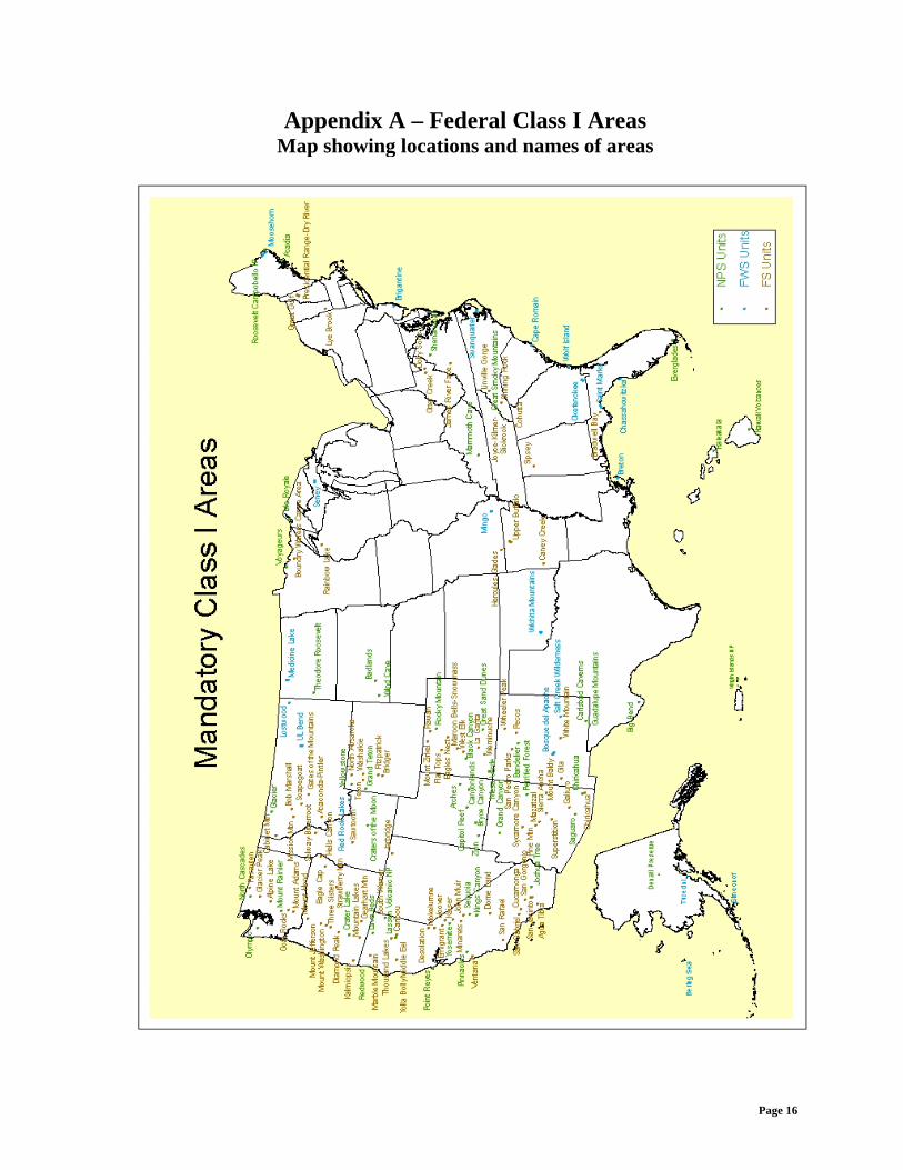
Appendix A – Federal Class I Areas Map showing locations and names of areas
Page 16
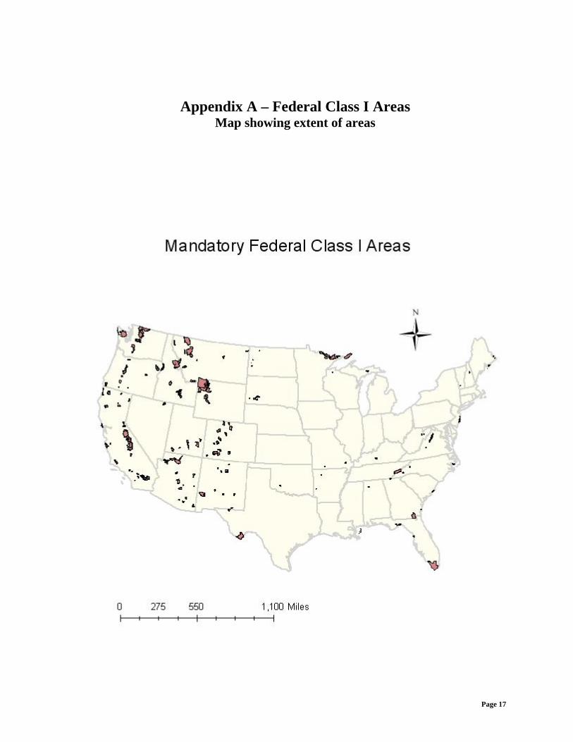
Appendix A – Federal Class I Areas Map showing extent of areas
Page 17
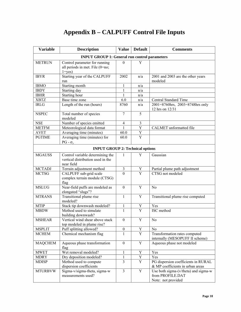
Appendix B – CALPUFF Control File Inputs
Variable Description Value Default Comments
INPUT GROUP 1: General run control parameters METRUN Control parameter for running
all periods in met. File (0=no; 1=yes)
0 Y
IBYR Starting year of the CALPUFF run
2002 n/a 2001 and 2003 are the other years modeled
IBMO Starting month 1 n/a IBDY Starting day 1 n/a IBHR Starting hour 1 n/a XBTZ Base time zone 6.0 n/a Central Standard Time IRLG Length of the run (hours) 8760 n/a 2001=8760hrs, 2003=8748hrs only
12 hrs on 12/31 NSPEC Total number of species
modeled 7 5
NSE Number of species emitted 4 3 METFM Meteorological data format 1 Y CALMET unformatted file AVET Averaging time (minutes) 60.0 Y PGTIME Averaging time (minutes) for
PG - σy
60.0 Y
INPUT GROUP 2: Technical options MGAUSS Control variable determining the
vertical distribution used in the near field
1 Y Gaussian
MCTADJ Terrain adjustment method 3 Y Partial plume path adjustment MCTSG CALPUFF sub-grid scale
complex terrain module (CTSG) flag
0 Y CTSG not modeled
MSLUG Near-field puffs are modeled as elongated “slugs”?
0 Y No
MTRANS Transitional plume rise modeled?
1 Y Transitional plume rise computed
MTIP Stack tip downwash modeled? 1 Y Yes MBDW Method used to simulate
building downwash? 1 Y ISC method
MSHEAR Vertical wind shear above stack top modeled in plume rise?
0 Y No
MSPLIT Puff splitting allowed? 0 Y No MCHEM Chemical mechanism flag 1 Y Transformation rates computed
internally (MESOPUFF II scheme) MAQCHEM Aqueous phase transformation
flag 0 Y Aqueous phase not modeled
MWET Wet removal modeled? 1 Y Yes MDRY Dry deposition modeled? 1 Y Yes MDISP Method used to compute
dispersion coefficients 3 Y PG dispersion coefficients in RURAL
& MP coefficients in urban areas MTURBVW Sigma-v/sigma-theta, sigma-w
measurements used? 3 Y Use both sigma-(v/theta) and sigma-w
from PROFILE.DAT Note: not provided
Page 18
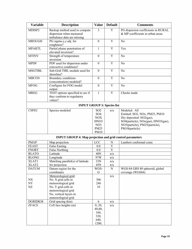
Variable Description Value Default Comments MDISP2 Backup method used to compute
dispersion when measured turbulence data are missing
3 Y PG dispersion coefficients in RURAL & MP coefficients in urban areas
MROUGH PG sigma-y,z adj. for roughness?
0 Y No
MPARTL Partial plume penetration of elevated inversion?
1 Y Yes
MTINV Strength of temperature inversion
0 Y No
MPDF PDF used for dispersion under convective conditions?
0 Y No
MSGTIBL Sub-Grid TIBL module used for shoreline?
0 Y No
MBCON Boundary conditions (concentration) modeled?
0 Y No
MFOG Configure for FOG model output
0 Y No
MREG TEST options specified to see if they conform to regulatory values?
1 Y Checks made
INPUT GROUP 3: Species list CSPEC Species modeled SO2
SO4 NOX
HNO3 NO3 PM25 PM10
n/a Modeled: All Emitted: SO2, NOx, PM25, PM10 Dry deposited: SO2(gas), SO4(particle), NOx(gas), HNO3(gas), NO3(particle), PM25(particle), PM10(particle)
INPUT GROUP 4: Map projection and grid control parameters PMAP Map projection LCC N Lambert conformal conic FEAST False Easting 0.0 Y FNORT False Northing 0.0 Y RLATO Latitude 40N n/a RLONG Longitude 97W n/a XLAT1 XLAT2
Matching parallel(s) of latitude for projection
33N 45N
n/a n/a
DATUM Datum region for the coordinates
WGS-G
N WGS-84 GRS 80 spheroid, global coverage (WGS84)
NX NY NZ
Meteorological grid: No. X grid cells in meteorological grid No. Y grid cells in meteorological grid No. vertical layers in meteorological grid
306 246 10
n/a
DGRIDKM Grid spacing (km) 6 n/a ZFACE Cell face heights (m) 0, 20,
40,80, 160, 320, 640,
1200,
n/a
Page 19
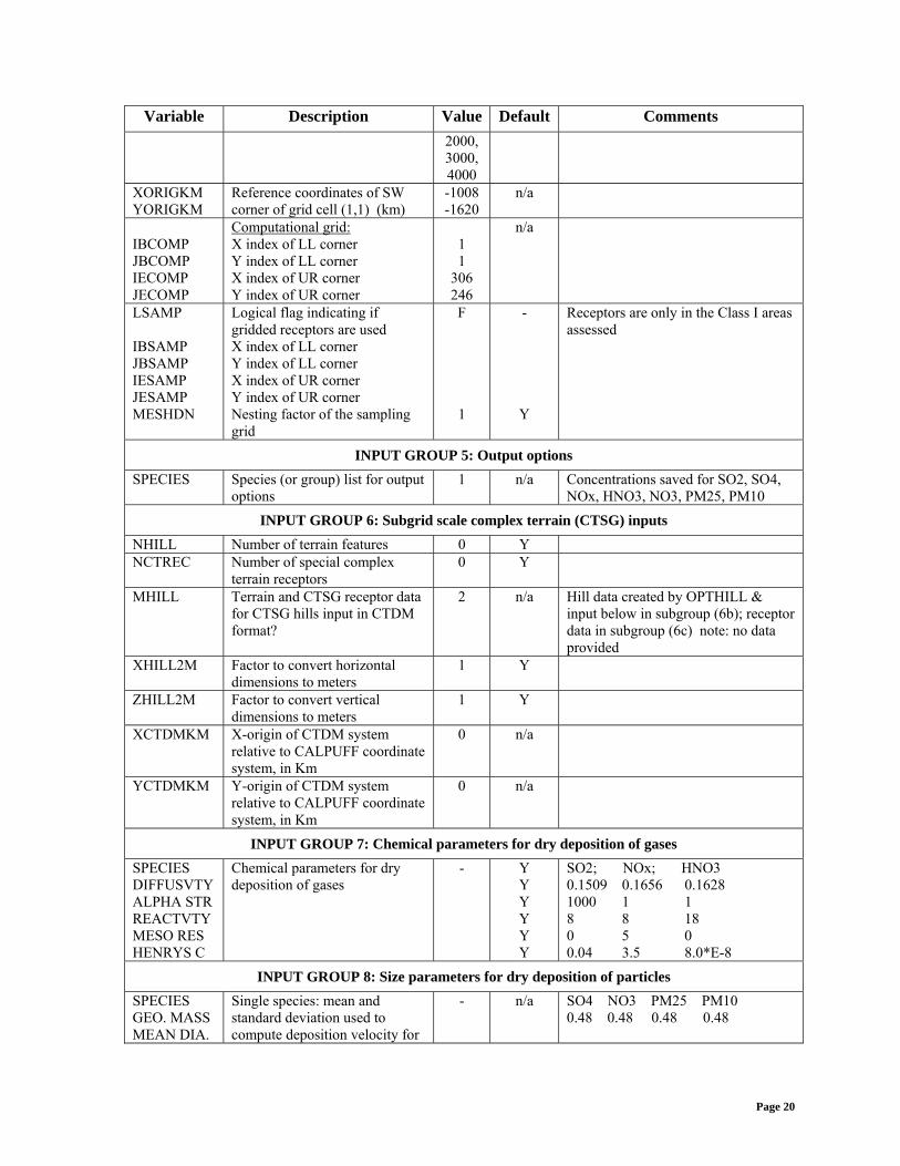
Variable Description Value Default Comments 2000, 3000, 4000
XORIGKM YORIGKM
Reference coordinates of SW corner of grid cell (1,1) (km)
-1008 -1620
n/a
IBCOMP JBCOMP IECOMP JECOMP
Computational grid: X index of LL corner Y index of LL corner X index of UR corner Y index of UR corner
1 1
306 246
n/a
LSAMP IBSAMP JBSAMP IESAMP JESAMP MESHDN
Logical flag indicating if gridded receptors are used X index of LL corner Y index of LL corner X index of UR corner Y index of UR corner Nesting factor of the sampling grid
F
1
-
Y
Receptors are only in the Class I areas assessed
INPUT GROUP 5: Output options SPECIES Species (or group) list for output
options 1 n/a Concentrations saved for SO2, SO4,
NOx, HNO3, NO3, PM25, PM10
INPUT GROUP 6: Subgrid scale complex terrain (CTSG) inputs NHILL Number of terrain features 0 Y NCTREC Number of special complex
terrain receptors 0 Y
MHILL Terrain and CTSG receptor data for CTSG hills input in CTDM format?
2 n/a Hill data created by OPTHILL & input below in subgroup (6b); receptor data in subgroup (6c) note: no data provided
XHILL2M Factor to convert horizontal dimensions to meters
1 Y
ZHILL2M Factor to convert vertical dimensions to meters
1 Y
XCTDMKM X-origin of CTDM system relative to CALPUFF coordinate system, in Km
0 n/a
YCTDMKM Y-origin of CTDM system relative to CALPUFF coordinate system, in Km
0 n/a
INPUT GROUP 7: Chemical parameters for dry deposition of gases SPECIES DIFFUSVTY ALPHA STR REACTVTY MESO RES HENRYS C
Chemical parameters for dry deposition of gases
- Y Y Y Y Y Y
SO2; NOx; HNO3 0.1509 0.1656 0.1628 1000 1 1 8 8 18 0 5 0 0.04 3.5 8.0*E-8
INPUT GROUP 8: Size parameters for dry deposition of particles SPECIES GEO. MASS MEAN DIA.
Single species: mean and standard deviation used to compute deposition velocity for
- n/a SO4 NO3 PM25 PM10 0.48 0.48 0.48 0.48
Page 20
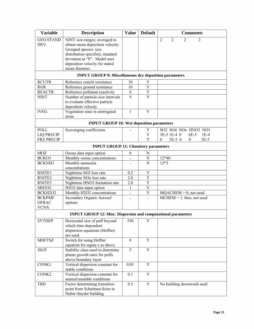
Variable Description Value Default Comments GEO.STAND DEV.
NINT size-ranges; averaged to obtain mean deposition velocity. Grouped species: size distribution specified, standard deviation as “0”. Model uses deposition velocity for stated mean diameter.
2 2 2 2
INPUT GROUP 9: Miscellaneous dry deposition parameters RCUTR Reference cuticle resistance 30 Y RGR Reference ground resistance 10 Y REACTR Reference pollutant reactivity 8 Y NINT Number of particle-size intervals
to evaluate effective particle deposition velocity
9 Y
IVEG Vegetation state in unirrigated areas
1 Y
INPUT GROUP 10: Wet deposition parameters POLL LIQ PRECIP FRZ PRECIP
Scavenging coefficients - Y Y Y
SO2 SO4 NOx HNO3 NO3 3E-5 1E-4 0 6E-5 1E-4 0 3E-5 0 0 3E-5
INPUT GROUP 11: Chemistry parameters MOZ Ozone data input option 0 N BCKO3 Monthly ozone concentrations - N 12*40 BCKNH3 Monthly ammonia
concentrations - N 12*3
RNITE1 Nighttime SO2 loss rate 0.2 Y RNITE2 Nighttime NOx loss rate 2.0 Y RNITE3 Nighttime HNO3 formation rate 2.0 Y MH2O2 H2O2 data input option 1 Y BCKH2O2 Monthly H2O2 concentrations - Y MQACHEM = 0; not used BCKPMF OFRAC VCNX
Secondary Organic Aerosol options
- - MCHEM = 1; thus, not used
INPUT GROUP 12: Misc. Dispersion and computational parameters SYTDEP Horizontal size of puff beyond
which time-dependent dispersion equations (Heffter) are used.
550 Y
MHFTSZ Switch for using Heffter equation for sigma z as above
0 Y
JSUP Stability class used to determine plume growth rates for puffs above boundary layer
5 Y
CONK1 Vertical dispersion constant for stable conditions
0.01 Y
CONK2 Vertical dispersion constant for neutral/unstable conditions
0.1 Y
TBD Factor determining transition-point from Schulman-Scire to Huber-Snyder building
0.5 Y No building downwash used
Page 21
Variable Description Value Default Comments downwash scheme
IURB1 IURB2
Range of land use categories for which urban dispersion is assumed
10 19
Y Y
METFM=1; not used
ILANDUIN Land use category for modeling domain
- - METFM=1; not used
ZOIN Roughness length (m) for modeling domain
- - METFM=1; not used
XLAIIN Leaf area index for modeling domain
- - METFM=1; not used
ELEVIN Elevation above sea level - - METFM=1; not used XLATIN Latitude (degrees) for met
location - - METFM=1; not used
XLONIN Longitude (degrees) for met location
- - METFM=1; not used
ANEMHT Anemometer height (m) - - METFM=1; not used ISIGMAV Form of lateral turbulence data
in PROFILE.DAT 1 Y Read sigma-v
IMIXCTDM Choice of mixing heights - - METFM=1; not used XMXLEN Maximum length of a slug 1 Y XSAMLEN Maximum travel distance of a
puff/slug during one sampling step
1 Y
MXNEW Maximum number of slugs/puffs released from one source during one time step
99 Y
MXSAM Maximum number of sampling steps for one puff/slug during one time step
99 Y
NCOUNT Number of iterations used when computing the transport wind for a sampling step that includes gradual rise
2 Y
SYMIN Minimum sigma y for a new puff/slug
1 Y
SZMIN Minimum sigma z for a new puff/slug
1 Y
SVMIN SWMIN
Default minimum turbulence velocities sigma-v and sigma-w for each stability class
- Y A B C D E F .5 .5 .5 .5 .5 .5 .2 .12 .08 .06 .03 .016
CDIV Divergence criterion for dw/dz across puff used to initiate adjustment for horizontal convergence
0, 0 Y
WSCALM Minimum wind speed allowed for non-calm conditions. Used as minimum speed returned when using power-law extrapolation toward surface
0.5 Y
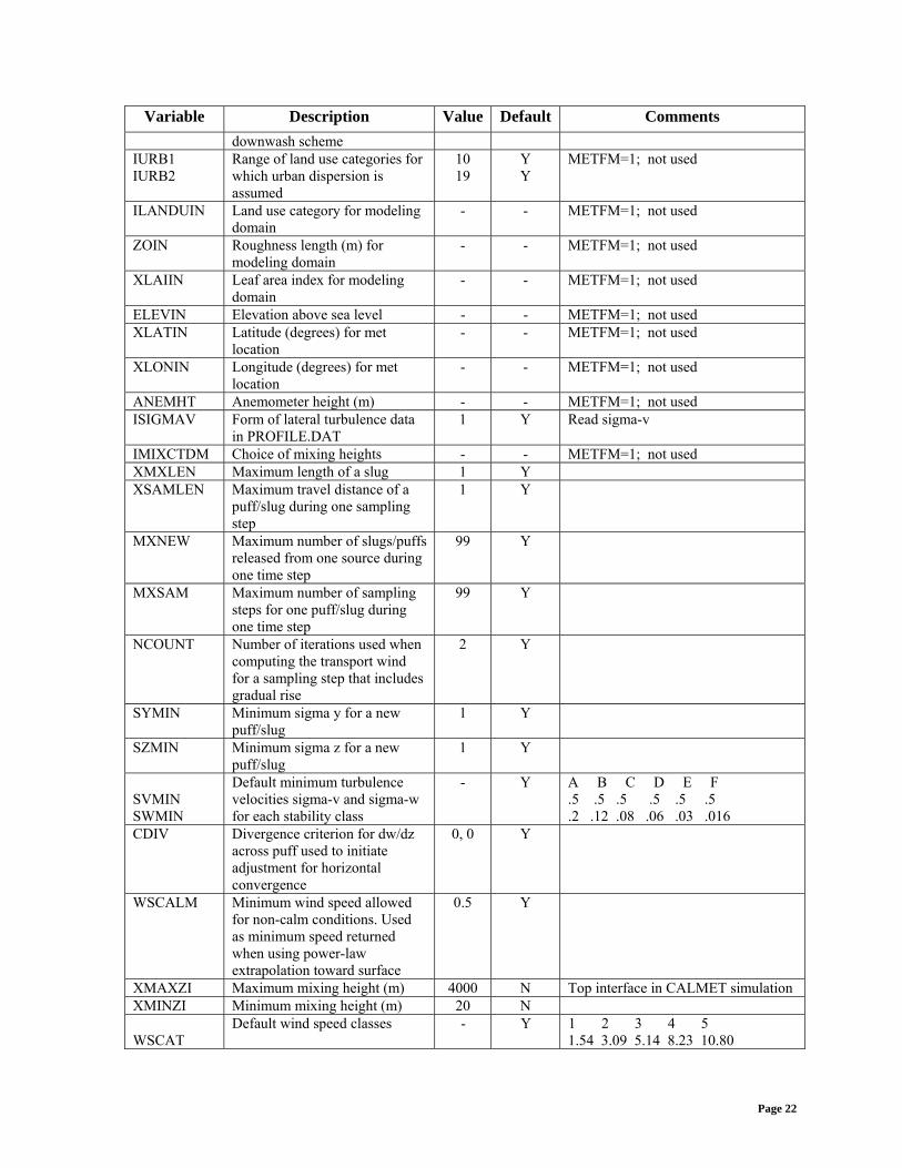
XMAXZI Maximum mixing height (m) 4000 N Top interface in CALMET simulation XMINZI Minimum mixing height (m) 20 N WSCAT
Default wind speed classes - Y 1 2 3 4 5 1.54 3.09 5.14 8.23 10.80
Page 22
Variable Description Value Default Comments PLXO
Default wind speed profile power-law exponents for stabilities 1-6
- Y ISC
RURAL
A B C D E F .07 .07 .10 .15 .35 .55
PTGO Default potential temperature gradient for stable classes E, F (deg K/m)
- Y 0.020; 0.035
PPC Default plume path coefficients for each stability class
- Y A B C D E F .5 .5 .5 .5 .35 .35
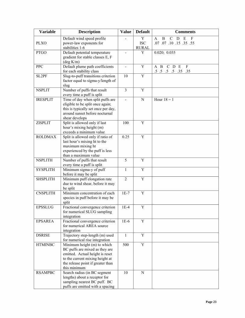
SL2PF Slug-to-puff transitions criterion factor equal to sigma-y/length of slug
10 Y
NSPLIT Number of puffs that result every time a puff is split
3 Y
IRESPLIT Time of day when split puffs are eligible to be split once again; this is typically set once per day, around sunset before nocturnal shear develops
- N Hour 18 = 1
ZISPLIT Split is allowed only if last hour’s mixing height (m) exceeds a minimum value
100 Y
ROLDMAX Split is allowed only if ratio of last hour’s mixing ht to the maximum mixing ht experienced by the puff is less than a maximum value
0.25 Y
NSPLITH Number of puffs that result every time a puff is split
5 Y
SYSPLITH Minimum sigma-y of puff before it may be split
1 Y
SHSPLITH Minimum puff elongation rate due to wind shear, before it may be split
2 Y
CNSPLITH Minimum concentration of each species in puff before it may be split
1E-7 Y
EPSSLUG Fractional convergence criterion for numerical SLUG sampling integration
1E-4 Y
EPSAREA Fractional convergence criterion for numerical AREA source integration
1E-6 Y
DSRISE Trajectory step-length (m) used for numerical rise integration
1 Y
HTMINBC Minimum height (m) to which BC puffs are mixed as they are emitted. Actual height is reset to the current mixing height at the release point if greater than this minimum
500 Y
RSAMPBC Search radius (in BC segment lengths) about a receptor for sampling nearest BC puff. BC puffs are emitted with a spacing
10 N
Page 23
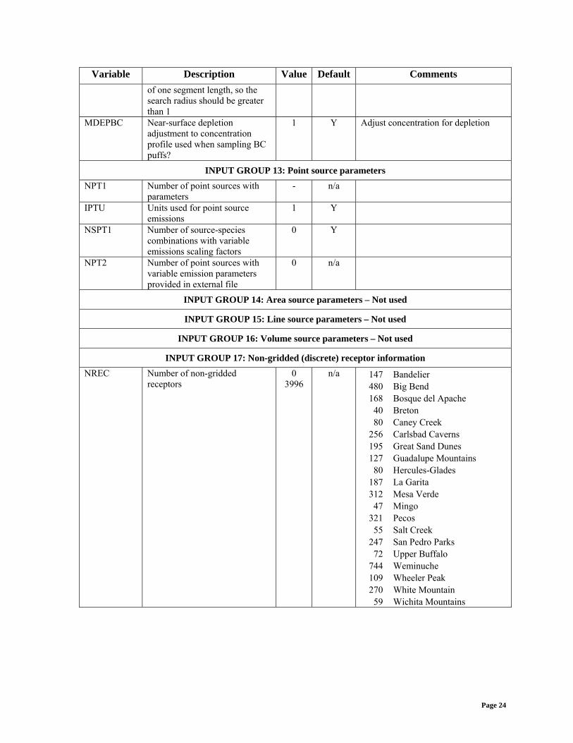
Variable Description Value Default Comments of one segment length, so the search radius should be greater than 1
MDEPBC Near-surface depletion adjustment to concentration profile used when sampling BC puffs?
1 Y Adjust concentration for depletion
INPUT GROUP 13: Point source parameters NPT1 Number of point sources with
parameters - n/a
IPTU Units used for point source emissions
1 Y
NSPT1 Number of source-species combinations with variable emissions scaling factors
0 Y
NPT2 Number of point sources with variable emission parameters provided in external file
0 n/a
INPUT GROUP 14: Area source parameters – Not used
INPUT GROUP 15: Line source parameters – Not used
INPUT GROUP 16: Volume source parameters – Not used
INPUT GROUP 17: Non-gridded (discrete) receptor information NREC Number of non-gridded
receptors 0
3996 n/a 147 Bandelier
480 Big Bend 168 Bosque del Apache 40 Breton 80 Caney Creek
256 Carlsbad Caverns 195 Great Sand Dunes 127 Guadalupe Mountains 80 Hercules-Glades
187 La Garita 312 Mesa Verde 47 Mingo
321 Pecos 55 Salt Creek
247 San Pedro Parks 72 Upper Buffalo
744 Weminuche 109 Wheeler Peak 270 White Mountain 59 Wichita Mountains
Page 24

Appendix C – POSTUTIL Control File Inputs
Variable Description Value Default Comments
INPUT GROUP 1: General run control parameters ISYR Starting Year 2002 n/a 2001 and 2003 also modeled ISMO Starting month 1 n/a IDY Starting day 1 n/a ISHR Starting hour 1 n/a NPER Number of periods to process 8760 n/a 2001=8760 hrs,
2003=8748hrs only 12 hrs on 12/31
NSPECINP Number of species to process from CALPUFF runs
7 n/a
NSPECOUT Number of species to write to output file 7 n/a NSPECCMP Number of species to compute from those
modeled 0 n/a
MDUPLCT Stop run if duplicate species names found?
0 Y
NSCALED Number of CALPUFF data files that will be scaled
0 Y
MNITRATE Re-compute the HNO3/NO3 partition for concentrations?
1 N Yes, for all sources combined
BCKNH3 Default ammonia concentrations used for HNO3/NO3 partition
- N 12*3
INPUT GROUP 2: Species processing information ASPECI NSPECINP species will be processed - n/a SO2, SO4, NOx, HNO3,
NO3, PM25, PM10 ASPECO NSPECOUT species will be written - n/a SO2, SO4, NOx, HNO3,
NO3, PM25, PM10
Page 25
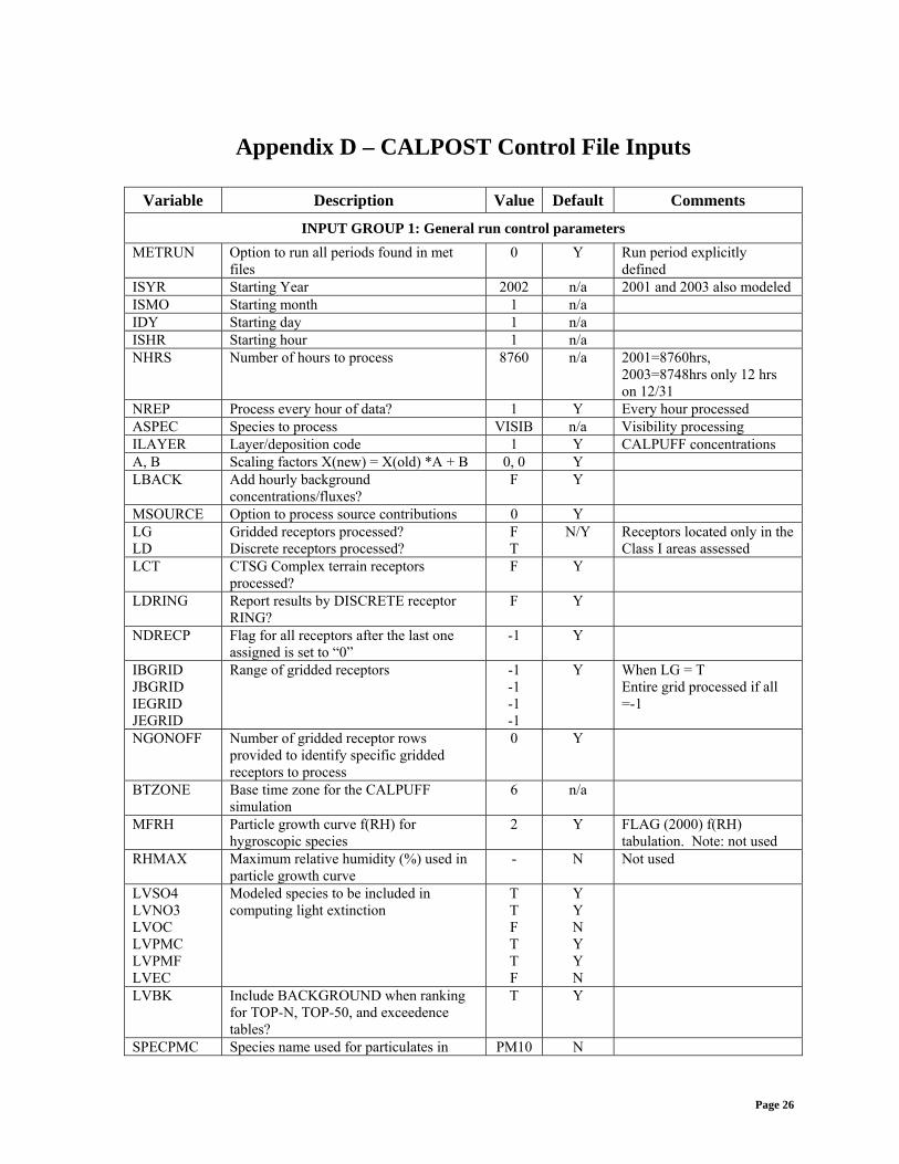
Appendix D – CALPOST Control File Inputs
Variable Description Value Default Comments
INPUT GROUP 1: General run control parameters METRUN Option to run all periods found in met
files 0 Y Run period explicitly
defined ISYR Starting Year 2002 n/a 2001 and 2003 also modeled ISMO Starting month 1 n/a IDY Starting day 1 n/a ISHR Starting hour 1 n/a NHRS Number of hours to process 8760 n/a 2001=8760hrs,
2003=8748hrs only 12 hrs on 12/31
NREP Process every hour of data? 1 Y Every hour processed ASPEC Species to process VISIB n/a Visibility processing ILAYER Layer/deposition code 1 Y CALPUFF concentrations A, B Scaling factors X(new) = X(old) *A + B 0, 0 Y LBACK Add hourly background
concentrations/fluxes? F Y
MSOURCE Option to process source contributions 0 Y LG LD
Gridded receptors processed? Discrete receptors processed?
F T
N/Y Receptors located only in the Class I areas assessed
LCT CTSG Complex terrain receptors processed?
F Y
LDRING Report results by DISCRETE receptor RING?
F Y
NDRECP Flag for all receptors after the last one assigned is set to “0”
-1 Y
IBGRID JBGRID IEGRID JEGRID
Range of gridded receptors -1 -1 -1 -1
Y When LG = T Entire grid processed if all =-1
NGONOFF Number of gridded receptor rows provided to identify specific gridded receptors to process
0 Y
BTZONE Base time zone for the CALPUFF simulation
6 n/a
MFRH Particle growth curve f(RH) for hygroscopic species
2 Y FLAG (2000) f(RH) tabulation. Note: not used
RHMAX Maximum relative humidity (%) used in particle growth curve
- N Not used
LVSO4 LVNO3 LVOC LVPMC LVPMF LVEC
Modeled species to be included in computing light extinction
T T F T T F
Y Y N Y Y N
LVBK Include BACKGROUND when ranking for TOP-N, TOP-50, and exceedence tables?
T Y
SPECPMC Species name used for particulates in PM10 N
Page 26
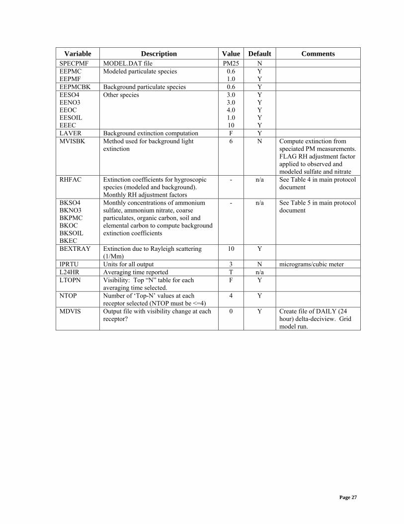
Variable Description Value Default Comments SPECPMF MODEL.DAT file PM25 N EEPMC EEPMF
Modeled particulate species 0.6 1.0
Y Y
EEPMCBK Background particulate species 0.6 Y EESO4 EENO3 EEOC EESOIL EEEC
Other species 3.0 3.0 4.0 1.0 10
Y Y Y Y Y
LAVER Background extinction computation F Y MVISBK Method used for background light
extinction 6 N Compute extinction from
speciated PM measurements. FLAG RH adjustment factor applied to observed and modeled sulfate and nitrate
RHFAC Extinction coefficients for hygroscopic species (modeled and background). Monthly RH adjustment factors
- n/a See Table 4 in main protocol document
BKSO4 BKNO3 BKPMC BKOC BKSOIL BKEC
Monthly concentrations of ammonium sulfate, ammonium nitrate, coarse particulates, organic carbon, soil and elemental carbon to compute background extinction coefficients
- n/a See Table 5 in main protocol document
BEXTRAY Extinction due to Rayleigh scattering (1/Mm)
10 Y
IPRTU Units for all output 3 N micrograms/cubic meter L24HR Averaging time reported T n/a LTOPN Visibility: Top “N” table for each
averaging time selected. F Y
NTOP Number of ‘Top-N’ values at each receptor selected (NTOP must be <=4)
4 Y
MDVIS Output file with visibility change at each receptor?
0 Y Create file of DAILY (24 hour) delta-deciview. Grid model run.
Page 27
BART Modeling E N V I R O N Huntsman Odessa Plant
ATTACHMENT B
30 TAC Chapter 116, Subchapter M: Best Available Retrofit Technology
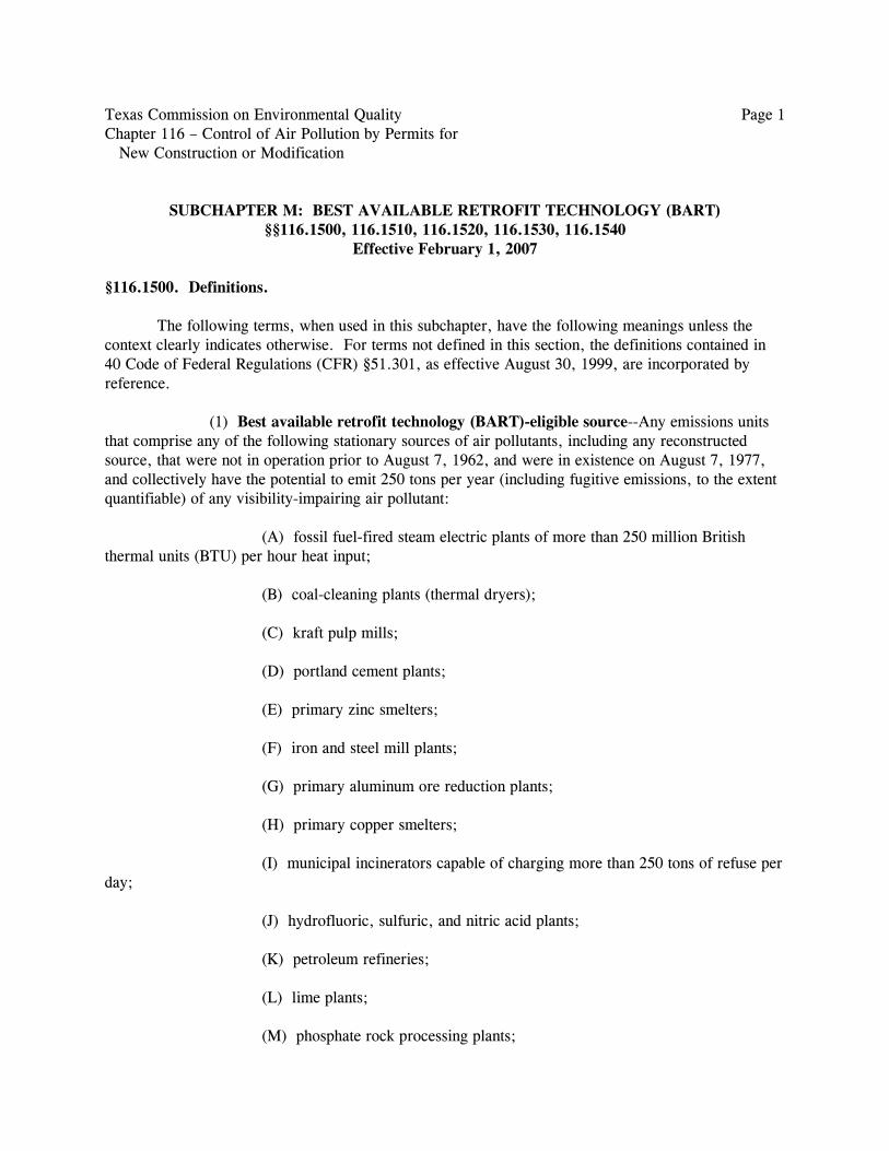
Texas Commission on Environmental Quality Page 1 Chapter 116 – Control of Air Pollution by Permits for New Construction or Modification
SUBCHAPTER M: BEST AVAILABLE RETROFIT TECHNOLOGY (BART) §§116.1500, 116.1510, 116.1520, 116.1530, 116.1540
Effective February 1, 2007
§116.1500. Definitions.
The following terms, when used in this subchapter, have the following meanings unless the context clearly indicates otherwise. For terms not defined in this section, the definitions contained in 40 Code of Federal Regulations (CFR) §51.301, as effective August 30, 1999, are incorporated by reference.
(1) Best available retrofit technology (BART)-eligible source--Any emissions units that comprise any of the following stationary sources of air pollutants, including any reconstructed source, that were not in operation prior to August 7, 1962, and were in existence on August 7, 1977, and collectively have the potential to emit 250 tons per year (including fugitive emissions, to the extent quantifiable) of any visibility-impairing air pollutant:
(A) fossil fuel-fired steam electric plants of more than 250 million British thermal units (BTU) per hour heat input;
(B) coal-cleaning plants (thermal dryers);
(C) kraft pulp mills;
(D) portland cement plants;
(E) primary zinc smelters;
(F) iron and steel mill plants;
(G) primary aluminum ore reduction plants;
(H) primary copper smelters;
(I) municipal incinerators capable of charging more than 250 tons of refuse per day;
(J) hydrofluoric, sulfuric, and nitric acid plants;
(K) petroleum refineries;
(L) lime plants;
(M) phosphate rock processing plants;

Texas Commission on Environmental Quality Page 2 Chapter 116 – Control of Air Pollution by Permits for New Construction or Modification
(N) coke oven batteries;
(O) sulfur recovery plants;
(P) carbon black plants (furnace process);
(Q) primary lead smelters;
(R) fuel conversion plants;
(S) sintering plants;
(T) secondary metal production facilities;
(U) chemical process plants;
(V) fossil fuel-fired boilers of more than 250 million BTUs per hour heat input;
(W) petroleum storage and transfer facilities with capacity exceeding 300,000 barrels;
(X) taconite ore processing facilities;
(Y) glass fiber processing plants; and
(Z) charcoal production facilities.
(2) Visibility-impairing air pollutant--Any of the following: nitrogen oxides, sulfur dioxide, or particulate matter.
Adopted January 10, 2007 Effective February 1, 2007
§116.1510. Applicability and Exemption Requirements.
(a) The requirements of this subchapter apply to best available retrofit technology (BART)-eligible sources as defined in §116.1500 of this title (relating to Definitions).
(b) The owner or operator of a BART-eligible source may demonstrate, using a model and modeling guidelines approved by the executive director, that the source does not contribute to visibility impairment at a Class I area. A BART-eligible source that does not contribute to visibility impairment at any Class I area is not subject to the requirements of §116.1520 or §116.1530 of this title (relating to Best Available Retrofit Technology (BART) Analysis and Best Available Retrofit Technology (BART) Control Implementation). A source is considered to not contribute to visibility impairment if, as
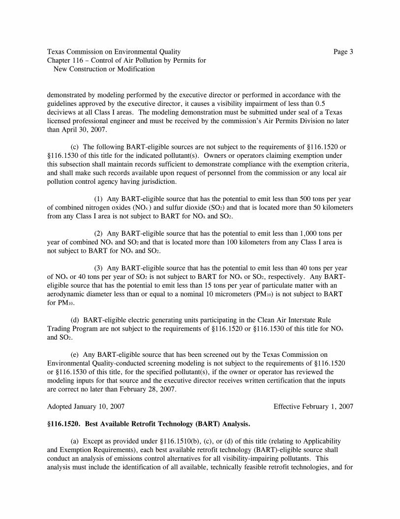
Texas Commission on Environmental Quality Page 3 Chapter 116 – Control of Air Pollution by Permits for New Construction or Modification
demonstrated by modeling performed by the executive director or performed in accordance with the guidelines approved by the executive director, it causes a visibility impairment of less than 0.5 deciviews at all Class I areas. The modeling demonstration must be submitted under seal of a Texas licensed professional engineer and must be received by the commission’s Air Permits Division no later than April 30, 2007.
(c) The following BART-eligible sources are not subject to the requirements of §116.1520 or §116.1530 of this title for the indicated pollutant(s). Owners or operators claiming exemption under this subsection shall maintain records sufficient to demonstrate compliance with the exemption criteria, and shall make such records available upon request of personnel from the commission or any local air pollution control agency having jurisdiction.
(1) Any BART-eligible source that has the potential to emit less than 500 tons per year of combined nitrogen oxides (NOx ) and sulfur dioxide (SO2) and that is located more than 50 kilometers from any Class I area is not subject to BART for NOx and SO2.
(2) Any BART-eligible source that has the potential to emit less than 1,000 tons per year of combined NOx and SO2 and that is located more than 100 kilometers from any Class I area is not subject to BART for NOx and SO2.
(3) Any BART-eligible source that has the potential to emit less than 40 tons per year of NOx or 40 tons per year of SO2 is not subject to BART for NOx or SO2, respectively. Any BART-eligible source that has the potential to emit less than 15 tons per year of particulate matter with an aerodynamic diameter less than or equal to a nominal 10 micrometers (PM10) is not subject to BART for PM10.
(d) BART-eligible electric generating units participating in the Clean Air Interstate Rule Trading Program are not subject to the requirements of §116.1520 or §116.1530 of this title for NOx
and SO2.
(e) Any BART-eligible source that has been screened out by the Texas Commission on Environmental Quality-conducted screening modeling is not subject to the requirements of §116.1520 or §116.1530 of this title, for the specified pollutant(s), if the owner or operator has reviewed the modeling inputs for that source and the executive director receives written certification that the inputs are correct no later than February 28, 2007.
Adopted January 10, 2007 Effective February 1, 2007
§116.1520. Best Available Retrofit Technology (BART) Analysis.
(a) Except as provided under §116.1510(b), (c), or (d) of this title (relating to Applicability and Exemption Requirements), each best available retrofit technology (BART)-eligible source shall conduct an analysis of emissions control alternatives for all visibility-impairing pollutants. This analysis must include the identification of all available, technically feasible retrofit technologies, and for
Texas Commission on Environmental Quality Page 4 Chapter 116 – Control of Air Pollution by Permits for New Construction or Modification
each technology identified, an analysis of the cost of compliance, the energy and non-air quality environmental impacts, the degree of visibility improvement in affected Class I areas resulting from the use of the control technology, the remaining useful life of the source, and any existing control technology present at the source. Based on this analysis, the owner or operator shall identify an emission control strategy as the prospective BART control strategy for the source. The determination of BART must be made according to 40 Code of Federal Regulations Part 51, Appendix Y, as effective September 6, 2005.
(b) As part of the BART analysis required in subsection (a) of this section, the owner or operator shall include detailed information documenting the projected hourly and annual emission limits for the selected BART control strategy.
(c) The owner or operator of each BART-eligible source shall submit a completed BART analysis to the commission’s Air Permits Division under seal of a Texas licensed professional engineer. The completed BART analysis must be received by the commission’s Air Permits Division no later than April 30, 2007.
Adopted January 10, 2007 Effective February 1, 2007
§116.1530. Best Available Retrofit Technology (BART) Control Implementation.
(a) Each owner or operator of a best available retrofit technology (BART)-eligible source shall install and operate BART-required control equipment no later than five years after the United States Environmental Protection Agency has approved a Regional Haze State Implementation Plan for the State of Texas. Each owner or operator shall maintain the BART-required control equipment and establish procedures to ensure such equipment is properly and continuously operated and maintained.
(b) Prior to any installation of BART-required control equipment, each owner or operator of a BART-eligible source shall comply with the requirements under Subchapter B of this chapter (relating to New Source Review Permits), Subchapter F of this chapter (relating to Standard Permits) or Subchapter H of this chapter (relating to Permits for Grandfathered Facilities) as applicable to authorize the construction or modification and to establish emission limitations of BART.
Adopted January 10, 2007 Effective February 1, 2007
Texas Commission on Environmental Quality Page 5 Chapter 116 – Control of Air Pollution by Permits for New Construction or Modification
§116.1540. Exemption from Best Available Retrofit Technology (BART) Control Implementation.
The owner or operator of any best available retrofit technology (BART)-eligible source may apply for an exemption from the requirement to install, operate, and maintain BART-required control equipment, pursuant to the provisions of 40 Code of Federal Regulations §51.303. Any exemption request under this section requires initial approval from the executive director and final approval from the administrator of the United States Environmental Protection Agency (EPA). Exemption requests submitted to the EPA must be accompanied by written concurrence from the executive director.
Adopted January 10, 2007 Effective February 1, 2007
BART Modeling E N V I R O N Huntsman Odessa Plant
ATTACHMENT C
CALPUFF Control File Inputs

Group Paramater Description CALPUFF Input Default Comments
METRUN Control parameter for running all periods in met. File (0=no; 1=yes) 0 0
IBYR Starting year of the CALPUFF run 2002 N.A. 2001 and 2003 are the other years modeledIBMO Starting month 1 N.A.IBDY Starting day 1 N.A.IBHR Starting hour 0 N.A.XBTZ Base time zone 0 N.A. Greenwich Mean Time
IRLG Length of the run (hours) 8760 N.A. 2001=8760hrs, 2003=8748hrs only 12 hrs on 12/31
NSPEC Total number of species modeled 9 5NSE Number of species emitted 9 3METFM Meteorological data format 1 1 CALMET unformatted fileAVET Averaging time (minutes) 60 60PGTIME Averaging time (minutes) for PG - σ 60 60
MGAUSSControl variable determining the vertical distribution used in the near field
1 1 Gaussian
MCTADJ Terrain adjustment method 3 3 Partial plume path adjustment
MCTSG CALPUFF sub-grid scale complex terrain module (CTSG) flag 0 0 CTSG not modeled
MSLUG Near-field puffs are modeled as elongated "slugs"? 0 0 No
MTRANS Transitional plume rise modeled? 1 1 Transitional plume rise computedMTIP Stack tip downwash modeled? 1 1 Yes
MBDW Method used to simulate building downwash? 1 1 ISC method
MSHEAR Vertical wind shear above stack top modeled in plume rise? 0 0 No
MSPLIT Puff splitting allowed? 0 0 0=No
MCHEM Chemical mechanism flag 1 1 Transformation rates computed internally (MESOPUFF II scheme)
MAQCHEM Aqueous phase transformation flag 0 0 Aqueous phase not modeledMWET Wet removal modeled? 1 1 YesMDRY Dry deposition modeled? 1 1 Yes
MDISP Method used to compute dispersion coefficients 3 3 PG dispersion coefficients in RURAL & MP
coefficients in urban areas
MTURBVW Sigma-v/sigma theta, sigma-w measurements used? 3 3
Use both sigma-(v/theta) and sigma-w from PROFILE.DAT Note: not provided
MDISP2Backup method used to compute dispersion when measured turbulence data are missing
3 3 PG dispersion coefficients in RURAL & MP coefficients in urban areas
MROUGH PG sigma-y,z adj. for roughness? 0 0 No
MPARTL Partial plume penetration of elevated inversion? 1 1 Yes
MTINV Strength of temperature inversion 0 0 No
MPDF PDF used for dispersion under convective conditions? 0 0 No
MSGTIBL Sub-Grid TIBL module used for shoreline? 0 0 No
MBCON Boundary conditions (concentration) modeled? 0 0 No
MFOG Configure for FOG model output 0 0 No
MREG TEST options specified to see if they conform to regulatory values? 1 1 Checks made
3 CSPEC Species modeledSO2, SO4, NOX, HNO3, NO3, EC, OC (SOA), PM25, PM10
N.A. PM25=PMFPM10=PMC
1
2
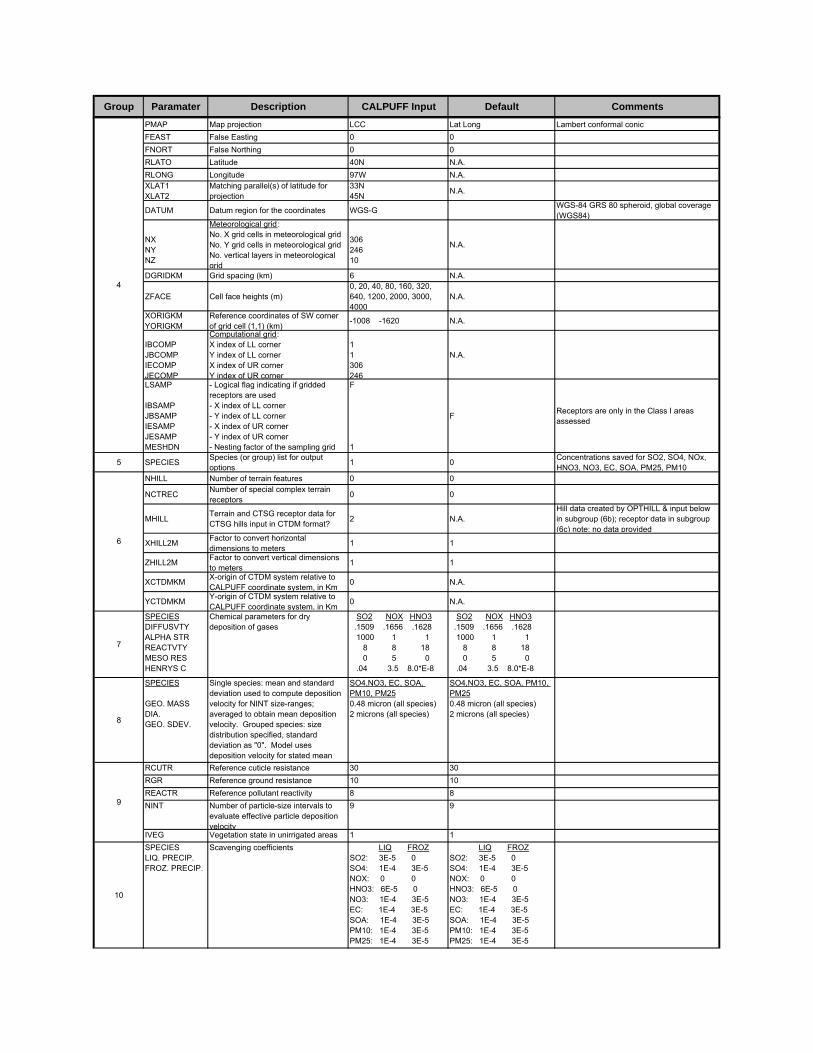
Group Paramater Description CALPUFF Input Default CommentsPMAP Map projection LCC Lat Long Lambert conformal conicFEAST False Easting 0 0FNORT False Northing 0 0RLATO Latitude 40N N.A.RLONG Longitude 97W N.A.XLAT1 XLAT2
Matching parallel(s) of latitude for projection
33N45N N.A.
DATUM Datum region for the coordinates WGS-G WGS-84 GRS 80 spheroid, global coverage (WGS84)
NXNYNZ
Meteorological grid :No. X grid cells in meteorological grid No. Y grid cells in meteorological gridNo. vertical layers in meteorological grid
30624610
N.A.
DGRIDKM Grid spacing (km) 6 N.A.
ZFACE Cell face heights (m)0, 20, 40, 80, 160, 320, 640, 1200, 2000, 3000, 4000
N.A.
XORIGKM YORIGKM
Reference coordinates of SW corner of grid cell (1,1) (km) -1008 -1620 N.A.
IBCOMPJBCOMPIECOMPJECOMP
Computational grid:X index of LL corner Y index of LL cornerX index of UR cornerY index of UR corner
11306246
N.A.
LSAMP
IBSAMPJBSAMPIESAMPJESAMPMESHDN
- Logical flag indicating if gridded receptors are used- X index of LL corner - Y index of LL corner - X index of UR corner - Y index of UR corner- Nesting factor of the sampling grid
F
1
F Receptors are only in the Class I areas assessed
5 SPECIES Species (or group) list for output options 1 0 Concentrations saved for SO2, SO4, NOx,
HNO3, NO3, EC, SOA, PM25, PM10NHILL Number of terrain features 0 0
NCTREC Number of special complex terrain receptors 0 0
MHILL Terrain and CTSG receptor data for CTSG hills input in CTDM format? 2 N.A.
Hill data created by OPTHILL & input below in subgroup (6b); receptor data in subgroup (6c) note: no data provided
XHILL2M Factor to convert horizontal dimensions to meters 1 1
ZHILL2M Factor to convert vertical dimensions to meters 1 1
XCTDMKM X-origin of CTDM system relative to CALPUFF coordinate system, in Km 0 N.A.
YCTDMKM Y-origin of CTDM system relative to CALPUFF coordinate system, in Km 0 N.A.
7
SPECIESDIFFUSVTYALPHA STRREACTVTYMESO RESHENRYS C
Chemical parameters for dry deposition of gases
SO2 NOX HNO3 .1509 .1656 .1628 1000 1 1 8 8 18 0 5 0 .04 3.5 8.0*E-8
SO2 NOX HNO3 .1509 .1656 .1628 1000 1 1 8 8 18 0 5 0 .04 3.5 8.0*E-8
8
SPECIES
GEO. MASS DIA.GEO. SDEV.
Single species: mean and standard deviation used to compute deposition velocity for NINT size-ranges; averaged to obtain mean deposition velocity. Grouped species: size distribution specified, standard deviation as "0". Model uses deposition velocity for stated mean
SO4,NO3, EC, SOA, PM10, PM250.48 micron (all species)2 microns (all species)
SO4,NO3, EC, SOA, PM10, PM250.48 micron (all species)2 microns (all species)
RCUTR Reference cuticle resistance 30 30RGR Reference ground resistance 10 10REACTR Reference pollutant reactivity 8 8NINT Number of particle-size intervals to
evaluate effective particle deposition velocity
9 9
IVEG Vegetation state in unirrigated areas 1 1
10
SPECIESLIQ. PRECIP.FROZ. PRECIP.
Scavenging coefficients LIQ FROZSO2: 3E-5 0SO4: 1E-4 3E-5NOX: 0 0HNO3: 6E-5 0NO3: 1E-4 3E-5EC: 1E-4 3E-5SOA: 1E-4 3E-5PM10: 1E-4 3E-5PM25: 1E-4 3E-5
LIQ FROZSO2: 3E-5 0SO4: 1E-4 3E-5NOX: 0 0HNO3: 6E-5 0NO3: 1E-4 3E-5EC: 1E-4 3E-5SOA: 1E-4 3E-5PM10: 1E-4 3E-5PM25: 1E-4 3E-5
4
6
9
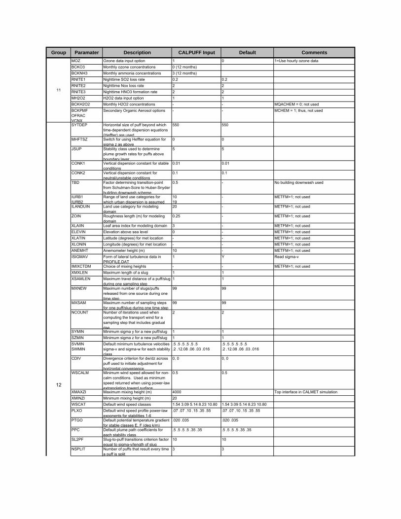
Group Paramater Description CALPUFF Input Default CommentsMOZ Ozone data input option 1 0 1=Use hourly ozone dataBCKO3 Monthly ozone concentrations 0 (12 months)BCKNH3 Monthly ammonia concentrations 3 (12 months)RNITE1 Nighttime SO2 loss rate 0.2 0.2RNITE2 Nighttime Nox loss rate 2 2RNITE3 Nighttime HNO3 formation rate 2 2MH2O2 H2O2 data input option 1 1BCKH2O2 Monthly H2O2 concentrations - - MQACHEM = 0; not usedBCKPMF OFRAC VCNX
Secondary Organic Aerosol options - - MCHEM = 1; thus, not used
SYTDEP Horizontal size of puff beyond which time-dependent dispersion equations (Heffter) are used.
550 550
MHFTSZ Switch for using Heffter equation for sigma z as above
0 0
JSUP Stability class used to determine plume growth rates for puffs above boundary layer
5 5
CONK1 Vertical dispersion constant for stable conditions
0.01 0.01
CONK2 Vertical dispersion constant for neutral/unstable conditions
0.1 0.1
TBD Factor determining transition-point from Schulman-Scire to Huber-Snyder building downwash scheme
0.5 - No building downwash used
IURB1IURB2
Range of land use categories for which urban dispersion is assumed
10 19
- METFM=1; not used
ILANDUIN Land use category for modeling domain
20 - METFM=1; not used
ZOIN Roughness length (m) for modeling domain
0.25 - METFM=1; not used
XLAIIN Leaf area index for modeling domain 3 - METFM=1; not usedELEVIN Elevation above sea level 0 - METFM=1; not usedXLATIN Latitude (degrees) for met location - - METFM=1; not usedXLONIN Longitude (degrees) for met location - - METFM=1; not usedANEMHT Anemometer height (m) 10 - METFM=1; not usedISIGMAV Form of lateral turbulence data in
PROFILE.DAT1 Y Read sigma-v
IMIXCTDM Choice of mixing heights - - METFM=1; not usedXMXLEN Maximum length of a slug 1 1XSAMLEN Maximum travel distance of a puff/slug
during one sampling step1 1
MXNEW Maximum number of slugs/puffs released from one source during one time step
99 99
MXSAM Maximum number of sampling steps for one puff/slug during one time step
99 99
NCOUNT Number of iterations used when computing the transport wind for a sampling step that includes gradual rise
2 2
SYMIN Minimum sigma y for a new puff/slug 1 1SZMIN Minimum sigma z for a new puff/slug 1 1SVMIN SWMIN
Default minimum turbulence velocities sigma-v and sigma-w for each stability class
.5 .5 .5 .5 .5 .5
.2 .12.08 .06 .03 .016.5 .5 .5 .5 .5 .5.2 .12.08 .06 .03 .016
CDIV Divergence criterion for dw/dz across puff used to initiate adjustment for horizontal convergence
0, 0 0, 0
WSCALM Minimum wind speed allowed for non-calm conditions. Used as minimum speed returned when using power-law extrapolation toward surface
0.5 0.5
XMAXZI Maximum mixing height (m) 4000 Top interface in CALMET simulationXMINZI Minimum mixing height (m) 20WSCAT Default wind speed classes 1.54 3.09 5.14 8.23 10.80 1.54 3.09 5.14 8.23 10.80PLXO Default wind speed profile power-law
exponents for stabilities 1-6.07 .07 .10 .15 .35 .55 .07 .07 .10 .15 .35 .55
PTGO Default potential temperature gradient for stable classes E, F (deg k/m)
.020 .035 .020 .035
PPC Default plume path coefficients for each stability class
.5 .5 .5 .5 .35 .35 .5 .5 .5 .5 .35 .35
SL2PF Slug-to-puff transitions criterion factor equal to sigma-y/length of slug
10 10
NSPLIT Number of puffs that result every time a puff is split
3 3
11
12
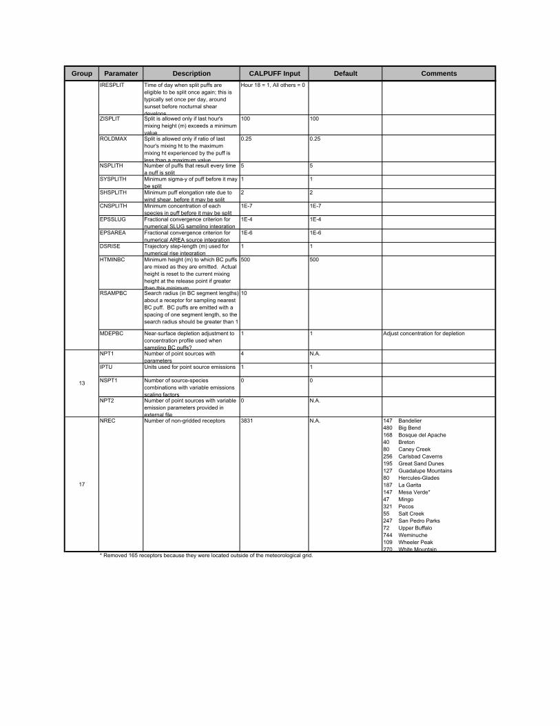
Group Paramater Description CALPUFF Input Default CommentsIRESPLIT Time of day when split puffs are
eligible to be split once again; this is typically set once per day, around sunset before nocturnal shear develops
Hour 18 = 1, All others = 0
ZISPLIT Split is allowed only if last hour's mixing height (m) exceeds a minimum value
100 100
ROLDMAX Split is allowed only if ratio of last hour's mixing ht to the maximum mixing ht experienced by the puff is less than a maximum value
0.25 0.25
NSPLITH Number of puffs that result every time a puff is split
5 5
SYSPLITH Minimum sigma-y of puff before it may be split
1 1
SHSPLITH Minimum puff elongation rate due to wind shear, before it may be split
2 2
CNSPLITH Minimum concentration of each species in puff before it may be split
1E-7 1E-7
EPSSLUG Fractional convergence criterion for numerical SLUG sampling integration
1E-4 1E-4
EPSAREA Fractional convergence criterion for numerical AREA source integration
1E-6 1E-6
DSRISE Trajectory step-length (m) used for numerical rise integration
1 1
HTMINBC Minimum height (m) to which BC puffs are mixed as they are emitted. Actual height is reset to the current mixing height at the release point if greater than this minimum
500 500
RSAMPBC Search radius (in BC segment lengths) about a receptor for sampling nearest BC puff. BC puffs are emitted with a spacing of one segment length, so the search radius should be greater than 1
10
MDEPBC Near-surface depletion adjustment to concentration profile used when sampling BC puffs?
1 1 Adjust concentration for depletion
NPT1 Number of point sources with parameters
4 N.A.
IPTU Units used for point source emissions 1 1
NSPT1 Number of source-species combinations with variable emissions scaling factors
0 0
NPT2 Number of point sources with variable emission parameters provided in external file
0 N.A.
17
NREC Number of non-gridded receptors 3831 N.A. 147 Bandelier480 Big Bend168 Bosque del Apache40 Breton80 Caney Creek256 Carlsbad Caverns 195 Great Sand Dunes127 Guadalupe Mountains80 Hercules-Glades187 La Garita147 Mesa Verde*47 Mingo321 Pecos55 Salt Creek247 San Pedro Parks72 Upper Buffalo744 Weminuche109 Wheeler Peak270 White Mountain
* Removed 165 receptors because they were located outside of the meteorological grid.
13
BART Modeling E N V I R O N Huntsman Odessa Plant
ATTACHMENT D
POSTUTIL Control File Inputs
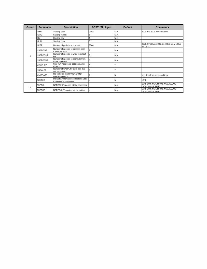
Group Paramater Description POSTUTIL Input Default CommentsISYR Starting year 2002 N.A. 2001 and 2003 also modeledISMO Starting month 1 N.A.IDY Starting day 1 N.A.ISHR Starting hour 0 N.A.
NPER Number of periods to process 8760 N.A. 2001=8760 hrs, 2003=8748 hrs (only 12 hrs on 12/31)
NSPECINP Number of species to process from CALPUFF runs 9 N.A.
NSPECOUT Number of species to write to output file 9 N.A.
NSPECCMP Number of species to compute from those modeled 0 N.A.
MDUPLCT Stop run if duplicate species names found? 0 Y
NSCALED Number of CALPUFF data files that will be scaled 0 Y
MNITRATE Re-compute the HNO3/NO3 for concentrations? 1 N Yes, for all sources combined
BCKNH3 Default ammonia concentrations used for HNO3/NO3 partition - N 12*3
ASPECI NSPECINP species will be processed - N.A. SO2, SO4, NOx, HNO3, NO3, EC, OC (SOA), PM25, PM10
ASPECO NSPECOUT species will be written - N.A. SO2, SO4, NOx, HNO3, NO3, EC, OC (SOA), PM25, PM10
2
1
BART Modeling E N V I R O N Huntsman Odessa Plant
ATTACHMENT E
CALPOST Control File Inputs
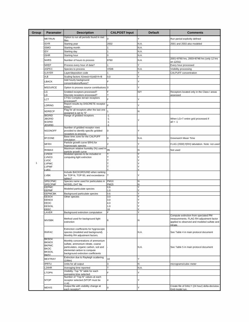
Group Paramater Description CALPOST Input Default Comments
METRUN Option to run all periods found in met files 0 Y Run period explicitly defined
ISYR Starting year 2002 N.A. 2001 and 2003 also modeledISMO Starting month 1 N.A.IDY Starting day 1 N.A.ISHR Starting hour 0 N.A.
NHRS Number of hours to process 8760 N.A. 2001=8760 hrs, 2003=8748 hrs (only 12 hrs on 12/31)
NREP Process every hour of data? 1 Y Every hour processedASPEC Species to process VISIB N.A. Visibility processingILAYER Layer/deposition code 1 Y CALPUFF concentrationA,B Scaling factors X(new)=X(old)*A+B 0,0 Y
LBACK Add hourly background concentrations/fluxes? F Y
MSOURCE Option to process source contributions 0 Y
LGLD
Gridded receptors processed?Discrete receptors processed?
FT
N/Y Receptors located only in the Class I areas assessed
LCT CTSG Complex terrain receptors processed? F Y
LDRING Report results by DISCRETE receptor RING? F Y
NDRECP Flag for all receptors after the last one assigned is set to "0" 1 N
IBGRIDJBGRIDIEGRIDJEGRID
Range of gridded receptors -1-1-1-1
Y When LG=T entire grid processed if all = -1
NGONOFFNumber of gridded receptor rows provided to identify specific gridded receptors to process
0 Y
BTZONE Base time zone for the CALPUFF simulation 0 N.A. Greenwich Mean Time
MFRH Particle growth curve f(RH) for hygroscopic species 2 Y FLAG (2000) f(RH) tabulation. Note: not used
RHMAX Maximum relative humidity (%) used in particle growth curve 95 N Not used
LVSO4LVNO3LVOCLVPMCLVPMFLVEC
Modeled species to be included in computing light extinction
TTTTTT
YYYYYY
LVBKInclude BACKGROUND when ranking for TOP-N, TOP-50, and exceedance tables?
T Y
SPECPMCSPECPMF
Species name used for particulates in MODEL.DAT file
PM10PM25
NN
EEPMCEEPMF Modeled particulate species 0.6
1.0YY
EEPMCBK Background particulate species 0.6 YEESO4EENO3EEOCEESOILEEEC
Other species 3.03.04.01.010
YYYYY
LAVER Background extinction computation F Y
MVISBK Method used for background light extinction 6 N
Compute extinction from speciated PM measurements. FLAG RH adjustment factor applied to observed and modeled sulfate and nitrate.
RHFACExtinction coefficients for hygroscopic species (modeled and background). Monthly RH adjustment factors.
- N.A. See Table 4 in main protocol document
BKSO4BKNO3BKPMCBKOCBKSOILBKEC
Monthly concentrations of ammonium sulfate, ammonium nitrate, coarse particulates, organic carbon, soil and elemental carbon to compute background extinction coefficients
- N.A. See Table 5 in main protocol document
BEXTRAY Extinction due to Rayleigh scattering (1/Mm) 10 Y
IPRTU Units for all output 3 N micrograms/cubic meterL24HR Averaging time reported T N.A.
LTOPN Visibility: Top "N" table for each averaging time selected. F Y
NTOPNumber of "Top-N" values at each receptor selected (NTOP must be <=4)
4 Y
MDVIS Output file with visibility change at each receptor? 0 Y Create file of DAILY (24 hour) delta-deciview.
Grid model run.
1

BART Modeling E N V I R O N Huntsman Odessa Plant
ATTACHMENT F
Modeling Archive
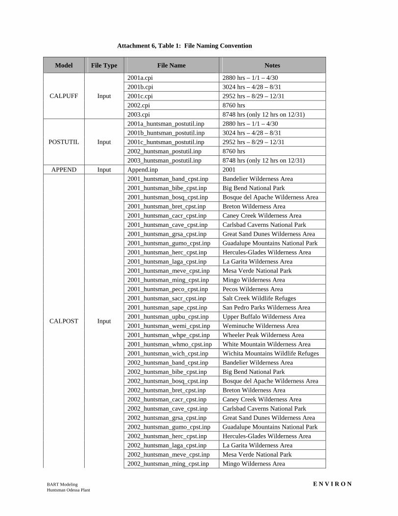
BART Modeling E N V I R O N Huntsman Odessa Plant
Attachment 6, Table 1: File Naming Convention
Model File Type File Name Notes
2001a.cpi 2880 hrs – 1/1 – 4/30 2001b.cpi 3024 hrs – 4/28 – 8/31 2001c.cpi 2952 hrs – 8/29 – 12/31 2002.cpi 8760 hrs
CALPUFF Input
2003.cpi 8748 hrs (only 12 hrs on 12/31) 2001a_huntsman_postutil.inp 2880 hrs – 1/1 – 4/30 2001b_huntsman_postutil.inp 3024 hrs – 4/28 – 8/31 2001c_huntsman_postutil.inp 2952 hrs – 8/29 – 12/31 2002_huntsman_postutil.inp 8760 hrs
POSTUTIL Input
2003_huntsman_postutil.inp 8748 hrs (only 12 hrs on 12/31) APPEND Input Append.inp 2001
2001_huntsman_band_cpst.inp Bandelier Wilderness Area 2001_huntsman_bibe_cpst.inp Big Bend National Park 2001_huntsman_bosq_cpst.inp Bosque del Apache Wilderness Area 2001_huntsman_bret_cpst.inp Breton Wilderness Area 2001_huntsman_cacr_cpst.inp Caney Creek Wilderness Area 2001_huntsman_cave_cpst.inp Carlsbad Caverns National Park 2001_huntsman_grsa_cpst.inp Great Sand Dunes Wilderness Area 2001_huntsman_gumo_cpst.inp Guadalupe Mountains National Park 2001_huntsman_herc_cpst.inp Hercules-Glades Wilderness Area 2001_huntsman_laga_cpst.inp La Garita Wilderness Area 2001_huntsman_meve_cpst.inp Mesa Verde National Park 2001_huntsman_ming_cpst.inp Mingo Wilderness Area 2001_huntsman_peco_cpst.inp Pecos Wilderness Area 2001_huntsman_sacr_cpst.inp Salt Creek Wildlife Refuges 2001_huntsman_sape_cpst.inp San Pedro Parks Wilderness Area 2001_huntsman_upbu_cpst.inp Upper Buffalo Wilderness Area 2001_huntsman_wemi_cpst.inp Weminuche Wilderness Area 2001_huntsman_whpe_cpst.inp Wheeler Peak Wilderness Area 2001_huntsman_whmo_cpst.inp White Mountain Wilderness Area 2001_huntsman_wich_cpst.inp Wichita Mountains Wildlife Refuges 2002_huntsman_band_cpst.inp Bandelier Wilderness Area 2002_huntsman_bibe_cpst.inp Big Bend National Park 2002_huntsman_bosq_cpst.inp Bosque del Apache Wilderness Area 2002_huntsman_bret_cpst.inp Breton Wilderness Area 2002_huntsman_cacr_cpst.inp Caney Creek Wilderness Area 2002_huntsman_cave_cpst.inp Carlsbad Caverns National Park 2002_huntsman_grsa_cpst.inp Great Sand Dunes Wilderness Area 2002_huntsman_gumo_cpst.inp Guadalupe Mountains National Park 2002_huntsman_herc_cpst.inp Hercules-Glades Wilderness Area 2002_huntsman_laga_cpst.inp La Garita Wilderness Area 2002_huntsman_meve_cpst.inp Mesa Verde National Park
CALPOST Input
2002_huntsman_ming_cpst.inp Mingo Wilderness Area
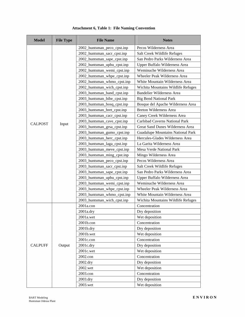
BART Modeling E N V I R O N Huntsman Odessa Plant
Attachment 6, Table 1: File Naming Convention
Model File Type File Name Notes
2002_huntsman_peco_cpst.inp Pecos Wilderness Area 2002_huntsman_sacr_cpst.inp Salt Creek Wildlife Refuges 2002_huntsman_sape_cpst.inp San Pedro Parks Wilderness Area 2002_huntsman_upbu_cpst.inp Upper Buffalo Wilderness Area 2002_huntsman_wemi_cpst.inp Weminuche Wilderness Area 2002_huntsman_whpe_cpst.inp Wheeler Peak Wilderness Area 2002_huntsman_whmo_cpst.inp White Mountain Wilderness Area 2002_huntsman_wich_cpst.inp Wichita Mountains Wildlife Refuges 2003_huntsman_band_cpst.inp Bandelier Wilderness Area 2003_huntsman_bibe_cpst.inp Big Bend National Park 2003_huntsman_bosq_cpst.inp Bosque del Apache Wilderness Area 2003_huntsman_bret_cpst.inp Breton Wilderness Area 2003_huntsman_cacr_cpst.inp Caney Creek Wilderness Area 2003_huntsman_cave_cpst.inp Carlsbad Caverns National Park 2003_huntsman_grsa_cpst.inp Great Sand Dunes Wilderness Area 2003_huntsman_gumo_cpst.inp Guadalupe Mountains National Park 2003_huntsman_herc_cpst.inp Hercules-Glades Wilderness Area 2003_huntsman_laga_cpst.inp La Garita Wilderness Area 2003_huntsman_meve_cpst.inp Mesa Verde National Park 2003_huntsman_ming_cpst.inp Mingo Wilderness Area 2003_huntsman_peco_cpst.inp Pecos Wilderness Area 2003_huntsman_sacr_cpst.inp Salt Creek Wildlife Refuges 2003_huntsman_sape_cpst.inp San Pedro Parks Wilderness Area 2003_huntsman_upbu_cpst.inp Upper Buffalo Wilderness Area 2003_huntsman_wemi_cpst.inp Weminuche Wilderness Area 2003_huntsman_whpe_cpst.inp Wheeler Peak Wilderness Area 2003_huntsman_whmo_cpst.inp White Mountain Wilderness Area
CALPOST Input
2003_huntsman_wich_cpst.inp Wichita Mountains Wildlife Refuges 2001a.con Concentration 2001a.dry Dry deposition 2001a.wet Wet deposition 2001b.con Concentration 2001b.dry Dry deposition 2001b.wet Wet deposition 2001c.con Concentration 2001c.dry Dry deposition 2001c.wet Wet deposition 2002.con Concentration 2002.dry Dry deposition 2002.wet Wet deposition 2003.con Concentration 2003.dry Dry deposition
CALPUFF Output
2003.wet Wet deposition
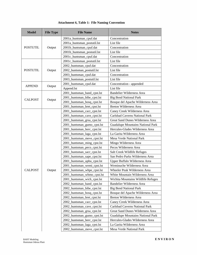
BART Modeling E N V I R O N Huntsman Odessa Plant
Attachment 6, Table 1: File Naming Convention
Model File Type File Name Notes
2001a_huntsman_cpuf.dat Concentration 2001a_huntsman_postutil.lst List file 2001b_huntsman_cpuf.dat Concentration 2001b_huntsman_postutil.lst List file
POSTUTIL Output
2001c_huntsman_cpuf.dat Concentration 2001c_huntsman_postutil.lst List file 2002_huntsman_cpuf.dat Concentration 2002_huntsman_postutil.lst List file 2003_huntsman_cpuf.dat Concentration
POSTUTIL Output
2003_huntsman_postutil.lst List file 2001_huntsman_cpuf.dat Concentration - appended
APPEND Output Append.lst List file 2001_huntsman_band_cpst.lst Bandelier Wilderness Area 2001_huntsman_bibe_cpst.lst Big Bend National Park 2001_huntsman_bosq_cpst.lst Bosque del Apache Wilderness Area
CALPOST Output
2001_huntsman_bret_cpst.lst Breton Wilderness Area 2001_huntsman_cacr_cpst.lst Caney Creek Wilderness Area 2001_huntsman_cave_cpst.lst Carlsbad Caverns National Park 2001_huntsman_grsa_cpst.lst Great Sand Dunes Wilderness Area 2001_huntsman_gumo_cpst.lst Guadalupe Mountains National Park 2001_huntsman_herc_cpst.lst Hercules-Glades Wilderness Area 2001_huntsman_laga_cpst.lst La Garita Wilderness Area 2001_huntsman_meve_cpst.lst Mesa Verde National Park 2001_huntsman_ming_cpst.lst Mingo Wilderness Area 2001_huntsman_peco_cpst.lst Pecos Wilderness Area 2001_huntsman_sacr_cpst.lst Salt Creek Wildlife Refuges 2001_huntsman_sape_cpst.lst San Pedro Parks Wilderness Area 2001_huntsman_upbu_cpst.lst Upper Buffalo Wilderness Area 2001_huntsman_wemi_cpst.lst Weminuche Wilderness Area 2001_huntsman_whpe_cpst.lst Wheeler Peak Wilderness Area 2001_huntsman_whmo_cpst.lst White Mountain Wilderness Area 2001_huntsman_wich_cpst.lst Wichita Mountains Wildlife Refuges 2002_huntsman_band_cpst.lst Bandelier Wilderness Area 2002_huntsman_bibe_cpst.lst Big Bend National Park 2002_huntsman_bosq_cpst.lst Bosque del Apache Wilderness Area 2002_huntsman_bret_cpst.lst Breton Wilderness Area 2002_huntsman_cacr_cpst.lst Caney Creek Wilderness Area 2002_huntsman_cave_cpst.lst Carlsbad Caverns National Park 2002_huntsman_grsa_cpst.lst Great Sand Dunes Wilderness Area 2002_huntsman_gumo_cpst.lst Guadalupe Mountains National Park 2002_huntsman_herc_cpst.lst Hercules-Glades Wilderness Area 2002_huntsman_laga_cpst.lst La Garita Wilderness Area
CALPOST Output
2002_huntsman_meve_cpst.lst Mesa Verde National Park
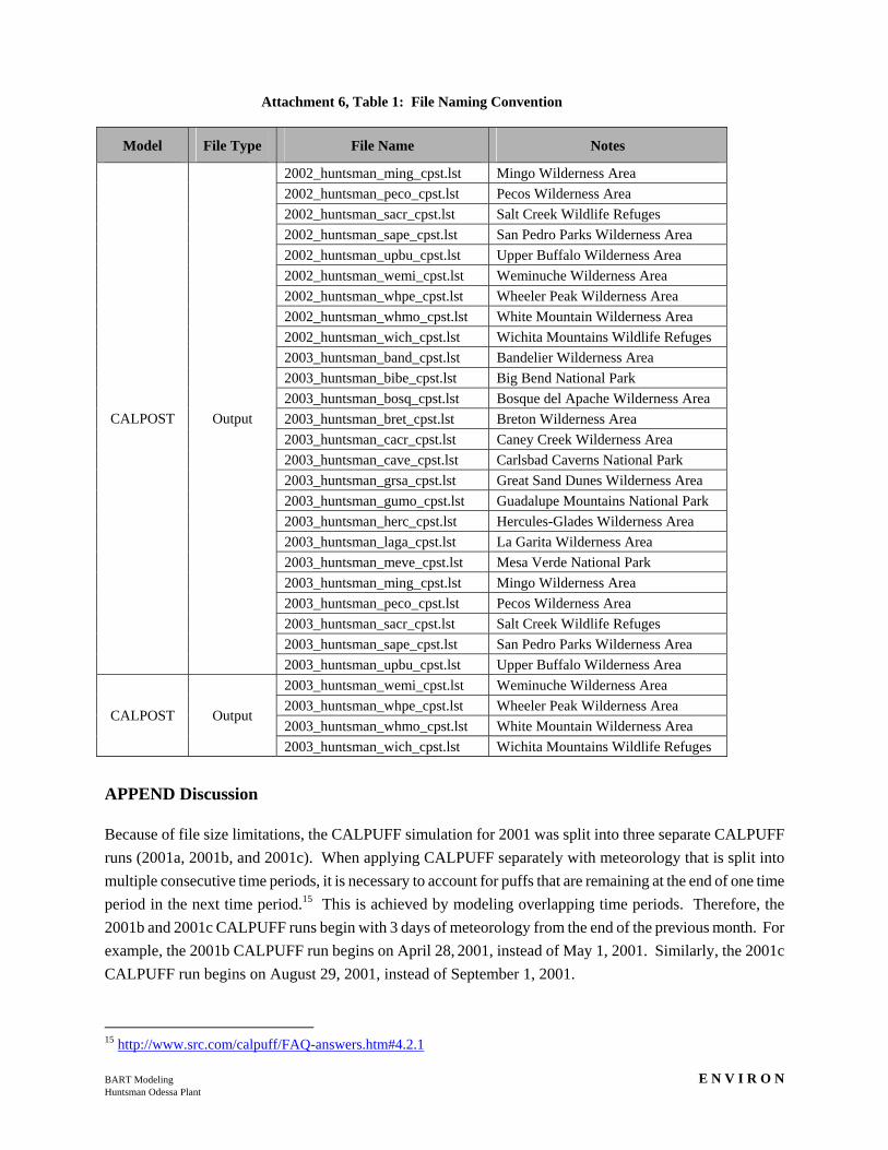
BART Modeling E N V I R O N Huntsman Odessa Plant
Attachment 6, Table 1: File Naming Convention
Model File Type File Name Notes
2002_huntsman_ming_cpst.lst Mingo Wilderness Area 2002_huntsman_peco_cpst.lst Pecos Wilderness Area 2002_huntsman_sacr_cpst.lst Salt Creek Wildlife Refuges 2002_huntsman_sape_cpst.lst San Pedro Parks Wilderness Area 2002_huntsman_upbu_cpst.lst Upper Buffalo Wilderness Area 2002_huntsman_wemi_cpst.lst Weminuche Wilderness Area 2002_huntsman_whpe_cpst.lst Wheeler Peak Wilderness Area 2002_huntsman_whmo_cpst.lst White Mountain Wilderness Area 2002_huntsman_wich_cpst.lst Wichita Mountains Wildlife Refuges 2003_huntsman_band_cpst.lst Bandelier Wilderness Area 2003_huntsman_bibe_cpst.lst Big Bend National Park 2003_huntsman_bosq_cpst.lst Bosque del Apache Wilderness Area 2003_huntsman_bret_cpst.lst Breton Wilderness Area 2003_huntsman_cacr_cpst.lst Caney Creek Wilderness Area 2003_huntsman_cave_cpst.lst Carlsbad Caverns National Park 2003_huntsman_grsa_cpst.lst Great Sand Dunes Wilderness Area 2003_huntsman_gumo_cpst.lst Guadalupe Mountains National Park 2003_huntsman_herc_cpst.lst Hercules-Glades Wilderness Area 2003_huntsman_laga_cpst.lst La Garita Wilderness Area 2003_huntsman_meve_cpst.lst Mesa Verde National Park 2003_huntsman_ming_cpst.lst Mingo Wilderness Area 2003_huntsman_peco_cpst.lst Pecos Wilderness Area 2003_huntsman_sacr_cpst.lst Salt Creek Wildlife Refuges 2003_huntsman_sape_cpst.lst San Pedro Parks Wilderness Area
CALPOST Output
2003_huntsman_upbu_cpst.lst Upper Buffalo Wilderness Area 2003_huntsman_wemi_cpst.lst Weminuche Wilderness Area 2003_huntsman_whpe_cpst.lst Wheeler Peak Wilderness Area 2003_huntsman_whmo_cpst.lst White Mountain Wilderness Area
CALPOST Output
2003_huntsman_wich_cpst.lst Wichita Mountains Wildlife Refuges
APPEND Discussion
Because of file size limitations, the CALPUFF simulation for 2001 was split into three separate CALPUFF runs (2001a, 2001b, and 2001c). When applying CALPUFF separately with meteorology that is split into multiple consecutive time periods, it is necessary to account for puffs that are remaining at the end of one time period in the next time period.15 This is achieved by modeling overlapping time periods. Therefore, the 2001b and 2001c CALPUFF runs begin with 3 days of meteorology from the end of the previous month. For example, the 2001b CALPUFF run begins on April 28, 2001, instead of May 1, 2001. Similarly, the 2001c CALPUFF run begins on August 29, 2001, instead of September 1, 2001.
15 http://www.src.com/calpuff/FAQ-answers.htm#4.2.1

BART Modeling E N V I R O N Huntsman Odessa Plant
The APPEND program can be used to append the sequential output data files into a single file for CALPOST processing. Output data files for 2001a, 2001b, and 2001c are appended to produce the 2001 output data file. Overlapping time periods are not a problem because the user can specify the number of hours to skip at the beginning and the total number of hours to read from each file. For this project, 72 hours (3 days) were skipped at the beginning of the 2001b and 2001c data files. The resulting output data file is 8760 hours in length.