Best Available Retrofit Technology (BART)

Modeling Protocol to Determine Sources Subject to BART in

the State of Minnesota

Draft October 10, 2005

Minnesota Pollution Control Agency 520 Lafayette Road North

St. Paul, Minnesota 55155-4194

aq-sip2-02

2

Table of Contents

Page No.

I. Introduction 3 II. Background 4 III. BART Air Quality Modeling Approach 5 IV. BART-Eligible Units 6 V. Physical Characteristics of BART-Eligible Units 9 A. Emissions 9 B. Stack Parameters 9 VI. Class I Areas to Assess 9 VII. Air Quality Model and Inputs 11 CALPUFF Modeling 11 A. Meteorological Data Modeling (CALMET) 13 B. Dispersion Modeling (CALPUFF) 15 C. Post Processing (CALPOST) 19 VIII. Visibility Impacts 20 IX. Change in Visibility due to BART Controls 22

aq-sip2-02

3

I. Introduction. On July 6, 2005, the U.S. Environmental Protection Agency (EPA) published final amendments to its 1999 regional haze rule in the Federal Register, including Appendix Y, the final guidance for Best Available Retrofit Technology (BART) determinations (70 FR 39104-39172). The BART rule requires the installation of BART on emission sources that fit specific criteria and “may reasonably be anticipated to cause or contribute” to visibility impairment in any Class I area. Air quality modeling is a means for determining who causes or contributes to visibility impairment. Minnesota’s proposed protocol for conducting this modeling for BART is provided herein. The Minnesota Pollution Control Agency (MPCA) foresees three purposes for this protocol. First, the MPCA will use the protocol to determine what BART-eligible units are subject-to-BART and must perform a BART determination. Second, facilities that the MPCA notifies are subject-to-BART will use this protocol to conduct modeling required when making BART determinations. Third, the MPCA will use this protocol to conduct modeling to show visibility impact on Class I areas, once the MPCA approves the BART emission limits for facilities subject-to-BART. This final modeling will be submitted to the EPA as part of the BART section of the Minnesota State Implementation Plan (SIP) for Regional Haze. New—both informal and formal—BART guidance continues to become available from the EPA and the Federal Land Managers (FLMs) that oversee visibility in Class I areas. Minnesota has developed a schedule for completing BART determinations and implementing the BART strategy in order to meet SIP deadlines. If the state is to meet those deadlines, modeling to determine sources subject-to-BART, and modeling to make BART determinations may need to be done before all new BART guidance from EPA and the FLMs becomes available. The MPCA intends to start modeling to determine sources subject-to-BART by the end of October. The MPCA will use the most current draft version of the protocol The draft should include all comments received and incorporated during the comment period for this draft (herein). The MPCA anticipates that it will notify sources subject-to-BART by December. The MPCA intends to provide guidance to facilities on making BART determinations at the beginning of January 2006. At that time, the MPCA intends to finalize the modeling protocol. The final protocol will include all available new EPA and FLM BART guidance as of that time. In the BART- determination guidance provided by the MPCA, facilities subject-to-BART will be directed to the final modeling protocol for making BART determinations. It is difficult at this time to know what new BART guidance may become available between the end of October and the beginning of January 2006.

aq-sip2-02

4

II. Background. Generally, Class I areas are national parks and wilderness areas in which visibility is more stringently protected under the Clean Air Act than any other areas in the United States. All the Class I areas are shown in Appendix A. Rainbow Lake Wilderness Area, a Class I area in Wisconsin, is shown on the map in Appendix A. However, it is not included in BART or other Regional Haze analyses because the FLMs have indicated that visibility is not a valuable feature of this Class I area. The BART requirements are a part of the SIP that will be submitted to EPA in late 2007. The SIP is a comprehensive plan of action to achieve reasonable progress goals to increase visibility in the Class I areas, and it is subject to approval by the EPA. The BART provisions are a part of the overall plan that focuses on reducing emissions from large sources that, due to age, were exempted from other control requirements in the Clean Air Act. An emissions source is considered eligible for BART if it falls into one of 26 listed categories, has the potential to emit at least 250 tons per year of any haze forming pollutant and existed on August 7, 1977, yet was not in operation before August 7, 1962. Thus, the BART provisions do not cover all sources that may cause or contribute to visibility impairment in any Class I area. According to the BART guidance, an individual source is considered to cause visibility impairment if it has a least a 1.0 deciview impact on the visiblity in a Class I area. A source is considered to contribute to visibility impairment if it has at least a 0.5 deciview impact. The final BART rule gives States discretion to establish a lower impact threshold than 0.5 deciviews. Although at this time the MPCA does not intend to establish a lower impact threshold, the MPCA has put this out for comment in a public notice dated September 6, 2005. For the purposes of this protocol, at this time the threshold will be considered 0.5 deciviews. The BART guidance allows a state to exempt individual sources from the BART requirements if they do not cause or contribute to any impairment of visibility in a Class I area. Exemption is done through air quality modeling. Although the BART guidance does not dictate how such an analysis must be done, it provides direction, which was used to develop this modeling protocol. The BART determination process includes many other steps in addition to the modeling described in this protocol. These steps—none of which are addressed in this document—include costs of compliance, energy and non-air quality impacts, existing pollution control technologies in use at the BART-eligible unit, remaining useful life of the units and improvements in visibility expected from the use of BART controls.

aq-sip2-02

5

III. BART Air Quality Modeling Approach. One of the air quality modeling approaches suggested by EPA in the BART guidance is an individual source attribution approach. This is the approach Minnesota proposes to take. Specifically, this entails modeling source-specific units and comparing modeled impacts to a particular deciview threshold (described above). Minnesota has decided to conduct the subject-to-BART modeling, rather than have each BART-eligible facility either conduct the modeling, or hire a contractor. This plan will eliminate the need for the State to quickly review many air quality modeling analyses conducted using varying approaches. This plan will also satisfy the need to use a consistent approach among the modeling analyses. Once the subject-to-BART modeling is complete, all the modeling inputs will be available to facilities subject-to-BART for them, or their consultants, to conduct modeling for making BART determinations. The modeling approach discussed here is specifically designed for conducting the BART analyses. There may be differences between acceptable modeling for conducting BART-analyses and that for conducting a visibility analysis for a New Source Review Permit; which may involve similar emission sources and the same air dispersion model used here. The State continues to refer New Source Review visibility modeling to the Federal Land Managers responsible for each of the Class I Areas in Minnesota. In preparing this modeling protocol, the State consulted BART modeling protocols drafted by other organizations to attain consistency. The three available draft BART modeling protocols consulted were the:

1. “Single Source Modeling to Support Regional Haze BART”, version 3, protocol developed by the Lake Michigan Air Directors Consortium (LADCO), Draft, September 6, 2005;

2. “Calpuff Modeling Protocol in Support of Best Available Retrofit Technology Determinations”, developed by the State of Iowa, Draft, August 2005; and

3. “Protocol for BART-Related Visibility Impairment Modeling Analyses in North Dakota”, developed by the State of North Dakota, Draft, September 2005.

This draft protocol is most similar to the LADCO and Iowa draft protocols, although North Dakota’s proposed method for determining natural background concentrations in each Class I area is proposed here. The LADCO protocol was reviewed by the National Park Service, EPA headquarters, and EPA Region V and addresses comments they had on earlier versions of the LADCO protocol. Minnesota is in EPA region V, and they will be reviewing Minnesota’s Regional Haze SIP of which BART will be a part. The Iowa DNR has indicated that they have not received comments on their protocol within their public comment period. North Dakota only recently made their draft protocol available for public comment. The Visibility Improvement State and Tribal Association of the Southeast states (VISTAS) has made its September 20, 2005, revised draft available, however, the MPCA has yet to review that document for consistency with this draft

aq-sip2-02

6

protocol. The MPCA intends to do this by the end of the comment period for this protocol. The MPCA intends to take several steps to complete the BART air quality modeling:

1. Send a Request For Information (RFI) to certain facilities in Minnesota and, from the response, determine the sources in Minnesota that fit the criteria for eligibility (Completed August 2005);

2. Extract the physical characteristics of the BART-eligible units from the RFI responses;

3. Determine which Class I areas to assess; 4. Choose an appropriate air quality model and develop inputs; 5. Conduct and post-process the subject-to-BART modeling and evaluate the

results: 6. Notify facilities subject-to-BART, and indicate that they use the final modeling

protocol and MPCA inputs while conducting modeling as part of their BART determinations;

7. Obtain emission limits and stack parameters resulting from BART determinations made by facilities subject-to-BART; and

8. Conduct follow-up modeling showing the difference between pre- and post-BART determinations.

IV. BART-Eligible Units. On July 28, 2005, the Minnesota Pollution Control Agency mailed to 130 facilities that are major for New Source Review a request for information about any BART-eligible units at their facility. Responses to that request indicate there are 25 facilities in Minnesota with BART-eligible units. The results are summarized in Table 1. Detailed information on the BART-eligible units based on their response to the RFI is provided in Appendix B (to be provided in the next version of this draft protocol). These are the sources that will undergo air quality modeling to determine whether the source must undergo an engineering analysis and possibly install the resulting BART. Figure 1 shows the facilities with BART-eligible units in relation to the two Class I areas in Minnesota, the Boundary Waters Canoe Area (BWCA) and Voyageurs National Park (Voyageurs).

aq-sip2-02

7

Figure 1. BART-eligible facilities in Minnesota.

EVTAC

New Ulm PUC

Hibbing PUCVirginia PUC

Sappi Cloquet

Rochester PUC

Gopher Resources

US Steel-Minntac

Hibbing Taconite

Marathon Ashland

Otter Tail Power

MN Power-Boswell

Austin Utilities

Boise White Paper

Xcel Energy-Sherco

Xcel Energy-Riverside

Southern MN Beet Sugar

MN Power-Taconite Harbor

Northshore Mining-Silver Bay

Flint Hills Resources-Pine Bend

American Crystal Sugar-E Grand For

BART-Eligible Minnesota Sources & Class I Areas

Legend

NPS Class IFWS Class IBART_Eligible SourcesFSminusRainbow

.

aq-sip2-02

Table 1. Facilities with BART-eligible Units BART Source Category Name

SIC Code

Facility ID Facility Name BART Emission Units as Identified by Facility

4931 2709900001 Austin Utilities NE Power Station

*Boiler No. 1 (EU001)

4931 2713700027 Hibbing Public Utilities

North boiler (EU003)

4911 2703100001 MN Power, Taconite Harbor

*Boiler no. 3 (EU003)

4911 2706100004 MN Power, Boswell Energy Center

*Boiler nos. 3 and possibly 4 (EU003, EU004)

4931 2701500010 New Ulm Public Utilities

No. 4 boiler (EU003)

4911 2711100002 Otter Tail Power Hoot Lake

*Unit 3 boiler (EU003)

4911 2710900011 Rochester Public Utilities, Silver Lake

Unit #3 boiler, *unit #4 boiler (EU003, EU004)

4911 2713700028 Virginia Public Utilities

Boiler no. 9 (EU003)

4911 2714100004 Xcel Energy, Sherco *Boilers 1 and 2 (EU001, EU002) 4911 2716300005 Xcel Energy, Allen S

King *Boiler 1 (EU001)

Fossil Fuel-fired Steam Electric Plants greater than 250 MMBtu/hour -- Electric Generating Units (EGUs)

4911 2705300015 Xcel Energy, Riverside

*Boiler 8 (EU003)

2911 2703700011 Flint Hills Resources LP – Pine Bend

15 emission units Petroleum Refineries

2911 2716300003 Marathon Ashland Petroleum LLC

24 emission units

1011 2713700113 EVTAC 54 emission units 1011 2713700061 Hibbing Taconite Co 29 emission units 1011 2713700062 Ispat Inland Mining 32 emission units 1011 2707500003 Northshore Mining,

Silver Bay 43 emission units (*EU002 potentially is CAIR EGU)

1011 2713700063 US Steel, Keewatin Taconite

32 emission units

Taconite Ore Processing Plants

1011 2713700005 US Steel, Minntac 375 emission units 2063 2711900002 American Crystal

Sugar, E. Gr. Forks Boilers 1 and 2 (EU001, EU002) Fossil fuel fired

boilers of more than 250 MMBTU/hr

2063 2712900014 Southern MN Beet Sugar

Boiler no. 1 (EU001)

2621 2707100002 Boise White Paper LLC, Intl Falls

#2 boiler, recovery furnace, smelt dissolving tank (EU340, EU320, EU322)

Kraft Pulp Mills

2611 2701700002 Sappi Cloquet, LLC #7, #8 power boilers (EU002, EU037)

Iron and Steel Mill Plants

3312 2712300055 Gerdau Ameristeel Reheat furnace (EU004)

Secondary Metal Production Facilities

3341 2703700016 Gopher Resources 3 emission units in reverberatory furnace area (EU003, EU007, EU008)

* Some Electric Generating Units are covered under the Clean Air Interstate Rule (CAIR). The BART guidance suggests that CAIR qualifies as better-than-BART. This suggestion has been put out for public comment. In the meantime, EGU’s covered under CAIR will be handled similarly to all other BART-eligible units in this modeling protocol.

aq-sip2-02

V. Physical Characteristics of BART-Eligible Units. A. Emissions. Emission data was obtained from facilities through the RFI described above. The State requested that the facilities submit emission data for nitrogen oxides (NOx), sulfur dioxide (SO2), particulate matter up to 10 microns in size (PM10) and particulate matter up to 2.5 microns in size (PM2.5). Emissions are reported in units of pounds per hour (lbs/hour) and reflect the maximum 24-hour actual emissions, as outlined in the BART guidance. This emission data will be used to model peak 24-hour averages for evaluating visiblity. The State does not intend to evaluate emissions of volatile organic compounds (VOCs) and ammonia from facilties. VOC emissions will not be evaluated because the necessary emission data has not been gathered. Only specific VOC compounds form secondary organic aerosols that affect visibility. These compounds are a fraction of the total VOCs reported in the emissions inventory. The MPCA does not have the breakdown of VOC emissions necessary to model those that only impair visibility. Even if Minnesota had this data, CALPUFF can not simulate formation of particles from anthropogenic VOC, nor its visibility impacts. Ammonia from specific sources will not be evaluated in this process, although ammonia is included in the modeling as a background concentration—this will be discussed later in this modeling protocol. The appropriate VOCs and ammonia emission data can, and will be, included in regional scale modeling used for the Regional Haze SIP. B. Stack parameters. Stack parameters for modeling were also obtained through the RFI described above. Parameters requested for each BART eligible unit were: height of the stack opening from ground, inside diameter, flow-rate, exit gas temperature, elevation of ground, and location coordinates of the stack. Because the modeling conducted for BART is concerned with long-range transport, not localized impacts, the RFI did not include data about building heights and widths that are used to calculate downwash. Details on the stack parameters to be used as inputs in the modeling are provided in Appendix B (to be provided in the next version of this draft protocol). VI. Class I Areas to Assess. There are two class I areas located in Minnesota, BWCA and Voyageurs. All facilities in Minnesota are located nearer to one of these two Class I areas than any other Class I areas. Thus, impacts of Minnesota facilities on BWCA and Voyageurs will be the focus of the BART visibility analysis. Impact to Class I areas in other states will be looked at in a broader sense, which will be described further below. The list of 10 Class I areas which will be included are depicted in Table 2. Figure 2 shows the location of each Class I area.

aq-sip2-02

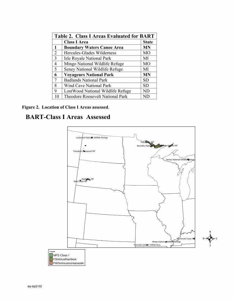
Table 2. Class I Areas Evaluated for BART Class I Area State 1 Boundary Waters Canoe Area MN 2 Hercules-Glades Wilderness MO 3 Isle Royale National Park MI 4 Mingo National Wildlife Refuge MO 5 Seney National Wildlife Refuge MI 6 Voyageurs National Park MN 7 Badlands National Park SD 8 Wind Cave National Park SD 9 LostWood National Wildlife Refuge ND 10 Theodore Roosevelt National Park ND

Figure 2. Location of Class I Areas assessed.

Voyageurs NP

Isle Royale NP

Badlands NP

Mammoth Cave NP

Theodore Roosevelt NP

Wind Cave NP

Boundry Waters Canoe Area

Hercules-Glades Wilderness

Seney National Wildlife Refuge

Mingo National Wildlife Refuge

Lostwood National Wildlife Refuge

BART-Class I Areas Assessed

Legend

NPS Class IFSminusRainbowFWSminusmontanasite

.

aq-sip2-02

VII. Air Quality Model and Inputs. According to EPA BART guidance, a State “can use CALPUFF, or another EPA approved model, to predict the visibility impacts from a single source at a Class I area.” For purposes of the BART determination, the MPCA intends to use CALPUFF. The MPCA recognizes that CALPUFF has limited ability to simulate the complex atmospheric chemistry involved in the estimation of secondary particulate formation. However, for purposes of the BART determination, the MPCA intends to use CALPUFF for the following reasons:

1. The increased level of effort required for conducting Particulate Matter Apportionment Technique in the regional scale full-chemistry eulerian model CAMx to acquire individual source contributions to Class I area, relative to the simplicity of the CALPUFF model;

2. The lack of a plume-in-grid feature with particulate apportionment technique currently available in CAMx;

3. The desire to be consistent with other states, which all—except perhaps Texas—appear to be using CALPUFF;

4. The limited scope of what this modeling is to determine (who must conduct an engineering analysis on various control options, and any perceived visibility difference with controls); and

5. The additional modeling of BART controls that will be conducted as part of the Regional Haze SIP with the CAMx model.

The EPA BART guidance states that States should follow the EPA’s Interagency Workgroup on Air Quality Modeling (IWAQM) guidance, Phase 2 recommendations, for long-range transport. The IWAQM guidance was developed to address air quality impacts—as assessed through the Prevention of Significant Deterioration (PSD) program—at Class I areas, where the source generally is located beyond 50 km of the Class I area. The IWAQM guidance does not specifically address the type of assessment that will occur with the BART analysis. As shown in Figure 1, above, Minnesota has BART-eligible units within 50 km of the class I areas: BWCA and Voyageurs. Based on limited verbal consultation with the National Park Service and the Forest Service, the MPCA will use the CALPUFF model for sources located within 50 km as well as beyond that distance. CALPUFF Modeling. Potentially, there will be three modeling scenarios. However, the third will only be applied if a modeling sensitivity test indicates that it is necessary. The scenarios and main features of each are as follows:

1. Sources within 50 km of the nearest Class I area ( 4 km CALPUFF/CALMET grid);

2. Sources further than 50 km from the nearest Class I area ( 12 km CALPUFF/CALMET grid); and

aq-sip2-02

12

3. Sources further than 250 km from the nearest Class I area if prescribed by sensitivity test ( 12 km CALPUFF/CALMET grid; with puff-splitting TO BE DETERMINED).

Modeling Domain. The CALPUFF modeling will be conducted on course- and fine-grid scales. The extent of the proposed 12 km and 4 km CALPUFF domains are shown in Figure 2. Using a finer 4-km grid for the nearest sources to the Class I areas will attempt to resolve issues associated with using CALPUFF within 50 km for visibility purposes. Figure 2. 12-km and 4 km CALPUFF domain .

Years Modeled. CALPUFF will be applied to each source for three annual simulations spanning the years 2002 through 2004. The IWAQM guidance allows the use of fewer than 5 years of meteorological data if a meteorological model using four-dimensional data assimilation is used to supply data. This is the case in this modeling analysis. See the section on meteorology for more information.

aq-sip2-02

13

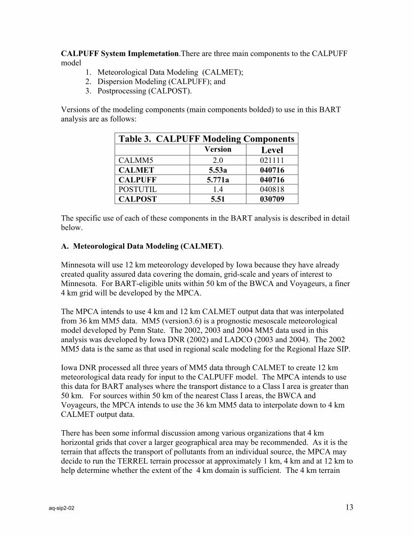
CALPUFF System Implemetation.There are three main components to the CALPUFF model

1. Meteorological Data Modeling (CALMET); 2. Dispersion Modeling (CALPUFF); and 3. Postprocessing (CALPOST).

Versions of the modeling components (main components bolded) to use in this BART analysis are as follows:

Table 3. CALPUFF Modeling Components Version Level CALMM5 2.0 021111 CALMET 5.53a 040716 CALPUFF 5.771a 040716 POSTUTIL 1.4 040818 CALPOST 5.51 030709

The specific use of each of these components in the BART analysis is described in detail below. A. Meteorological Data Modeling (CALMET). Minnesota will use 12 km meteorology developed by Iowa because they have already created quality assured data covering the domain, grid-scale and years of interest to Minnesota. For BART-eligible units within 50 km of the BWCA and Voyageurs, a finer 4 km grid will be developed by the MPCA. The MPCA intends to use 4 km and 12 km CALMET output data that was interpolated from 36 km MM5 data. MM5 (version3.6) is a prognostic mesoscale meteorological model developed by Penn State. The 2002, 2003 and 2004 MM5 data used in this analysis was developed by Iowa DNR (2002) and LADCO (2003 and 2004). The 2002 MM5 data is the same as that used in regional scale modeling for the Regional Haze SIP. Iowa DNR processed all three years of MM5 data through CALMET to create 12 km meteorological data ready for input to the CALPUFF model. The MPCA intends to use this data for BART analyses where the transport distance to a Class I area is greater than 50 km. For sources within 50 km of the nearest Class I areas, the BWCA and Voyageurs, the MPCA intends to use the 36 km MM5 data to interpolate down to 4 km CALMET output data. There has been some informal discussion among various organizations that 4 km horizontal grids that cover a larger geographical area may be recommended. As it is the terrain that affects the transport of pollutants from an individual source, the MPCA may decide to run the TERREL terrain processor at approximately 1 km, 4 km and at 12 km to help determine whether the extent of the 4 km domain is sufficient. The 4 km terrain

aq-sip2-02

14

developed for input to the CALMET modeling determines the CALMET-derived 4 km windfields To create the 4 km CALMET data, the MPCA will run the requisite pre-processors to CALMET: TERREL, a terrain pre-processor that averages terrain features to the modeling grid resolution; CTGPROC, which computes the fractional land use for the modeling grid resolution; and MAKEGEO, the final pre-processor that combines the terrain and land use data for input to CALMET. The MPCA will obtain CALMM5 output from the Iowa DNR. CALMM5 converts the MM5 data into a form compatible with CALMET. No observation data was used in the CALMET modeling. This means the prognostic meteorological data set from MM5 is not supplemented with surface or upper air observations. The use of observations is thought to counter-balance smoothing that may occur based on the grid-scale of the MM5 data. Neither LADCO nor Iowa DNR (and CenRAP; although no protocol is available) proposes to supplement the MM5 with observation data. Both LADCO and Iowa claim that because the observation data is included in the ETA analysis fields used to initialize MM5, adding observational data in CALMET is redundant. The prognostic model MM5 is designed to “fill in missing data around the surface monitoring network and sparse upper air monitoring network.” (LADCO). The CALMET control file contains the following options in order to reflect no observations:

♦ ICLOUD = 3; Gridded cloud cover from Prognostic Rel. Humidity (default is ICLOUD = 0; recommended by FLMs)

♦ IPROG = 14; Use winds from the MM5 output as initial guess field ♦ ITPROG = 2; No surface or upper air observations, use MM5

Another deviation from defaults is allowing the computation of kinematic effects in the wind field options and parameters. This was the case in the CALMET modeling. The control option for computing kinematic effects was turned on (IKINE = 1). Some BART-eligible units are located near Lake Superior. Although the FLMs have recommended the use of the “lake breeze module” for at least one PSD application in Minnesota—where the source is located near Lake Superior—the MPCA proposes not to use the option for the BART analysis. Appendix C contains a section of the Iowa DNR draft modeling protocol detailing the meteorological data included in this BART analysis. It includes the map projection and grid control parameters (for example, the Lambert Conformal Conic coordinate system is used). Although no comments were received during the Iowa public comment period, the document may still be subject to change due to any forthcoming comments from the National Park Service, Forest Service and EPA Region VII to Iowa.

aq-sip2-02

15

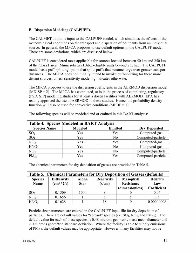
B. Dispersion Modeling (CALPUFF). The CALMET output is input to the CALPUFF model, which simulates the effects of the meteorological conditions on the transport and dispersion of pollutants from an individual source. In general, the MPCA proposes to use default options in the CALPUFF model. There are some deviations, which are discussed below. CALPUFF is considered most applicable for sources located between 50 km and 250 km of the Class I area. Minnesota has BART-eligible units beyond 250 km. The CALPUFF model has a puff-splitting option that splits puffs that become large over greater transport distances. The MPCA does not initially intend to invoke puff-splitting for these more distant sources, unless sensitivity modeling indicates otherwise. The MPCA proposes to use the dispersion coefficients in the AERMOD dispersion model (MDISP = 2). The MPCA has completed, or is in the process of completing, regulatory (PSD, SIP) modeling studies for at least a dozen facilities with AERMOD. EPA has readily approved the use of AERMOD in these studies. Hence, the probability density function will also be used for convective conditions (MPDF = 1). The following species will be modeled and or emitted in this BART analysis: Table 4. Species Modeled in BART Analysis

Species Name Modeled Emitted Dry Deposited SO2 Yes Yes Computed-gas SO4 Yes No Computed-particle NOX Yes Yes Computed-gas HNO3 Yes No Computed-gas NO3 Yes No Computed-particle PM2.5 Yes Yes Computed-particle The chemical parameters for dry deposition of gasses are provided in Table 5. Table 5. Chemical Parameters for Dry Deposition of Gasses (defaults)

Species Name

Diffusivity (cm**2/s)

Alpha Star

Reactivity (s/cm)

Mesophyll Resistance

(dimensionless)

Henry’s Law

Coefficient SO2 0.1509 1000 8 0 0.04 NOX 0.1656 1 8 5 3.5 HNO3 0.1628 1 18 0 0.00000008 Particle size parameters are entered in the CALPUFF input file for dry deposition of particles. There are default values for “aerosol” species (i.e. SO4, NO3, and PM2.5). The default value for each of these species is 0.48 microns geometric mass mean diameter and 2.0 microns geometric standard deviation. Where the facility is able to supply emissions of PM2.5, the default values may be appropriate. However, many facilities may not be

aq-sip2-02

16

able to supply PM2.5 emissions and will supply what is available; PM10 emissions. In this case, using the default values may underestimate deposition of particulates and overestimate the particulate contribution to visibility. For sources that did not report PM2.5 emissions in the RFI, the MPCA intends to scale PM10 emissions to PM2.5 using the PM2.5/ PM10 ratio calculated by the MPCA for the 2002 emissions inventory. The MPCA request for information described above did not request that sources indicate how much of their particulate emissions might be elemental carbon (EC) or secondary organic aerosol (SOA). The light extinction coefficient for PM2.5 is 1, EC is 10 and SOA is 4. Thus, EC and SOA will have a comparatively higher impact on visiblity. The main sources of these particles are fuel combustion. A way to account for this, without including EC and SOA in the modeling, is to use particle speciation in the post processing step. This is discussed below in the CALPOST section. Wet deposition parameters—which are defaults—are provided in Table 6.

Table 6. Wet Deposition Parameters (defaults). Scavenging Coefficient – (sec-1)

Pollutant Liquid Precipitation Frozen Precipitation SO2 3.0E-05 0.0E-00 SO4 1.0E-04 3.0E-05 HNO3 6.0E-05 0.0E-00 NO3 1.0E-04 3.0E-05 PM10 1.0E-04 3.0E-05

Ozone, ammonia and hydrogen peroxide concentrations are input to CALPUFF as monthly background values reflecting each—12 km and 4 km—modeling domain. The monthly values of ozone, ammonia and hydrogen peroxide concentrations were obtained from an annual CAMx4 model simulation for the year 2002, which was conducted by LADCO. The values were averaged over the size of the modeling domain, using tools developed by LADCO. Thus, the values input in the 12 km CALPUFF analysis will be those values averaged over the 12 km domain, and the values input in the 4 km CALPUFF analysis will be those values averaged over the 4 km domain. The background ozone, ammonia and hydrogen peroxide values used in this analysis are provided in Table 7.

aq-sip2-02

17

Table 7. Ozone, Ammonia and Hydrogen Peroxide Concentrations –Domain Seasonal Average—ppb Jan-

Mar Apr-Jun

Jul-Sep

Oct-Dec

Ozone 12 km domain 27.06 38.16 36.70 23.22

4 km domain 36.46 44.42 36.55 29.90

NH3 12 km domain 0.59 1.11 1.16 1.09

4 km domain 0.05 0.18 0.15 0.13

H2O2 12 km domain 0.32 2.23 3.54 0.47

4 km domain 0.25 2.08 3.33 0.30

Receptors are locations where model results are calculated and provided in the CALPUFF output files. Receptor locations were derived from National Park Service’s Class I area receptor database at http://www2.nature.nps.gov/air/maps/receptors/index.cfm. Two receptor applications will be modeled in CALPUFF. One with discrete receptors densely placed in the Class I areas BWCA and Voyageurs. The other with receptors located at the center of each grid on the 12 km grid domain. The discrete receptors are necessary for calculating visibility impacts in the selected Class I areas. All the discrete receptors will be placed with enough density that the highest visibility impacts should be evident. The NPS provides receptors in all the Class I areas on a 1 km basis. These receptors will be kept at the 1 km spacing for the BART modeling. Discrete receptor placement in the two Class I areas is shown in Figure 3.

aq-sip2-02

18

Figure 3. 1 km Receptor Placement in BWCA and Voyageurs.

Receptors placed at the center of each grid square will provide a broader scope of the impacts and will show the general impacts to Class I areas (see Table 2) in addition to the BWCA and Voyageurs. Receptors located within each 12-km grid cell will allow a tile plot to be created to display the extent of CALPUFF modeling impacts in all directions. Receptor placement is shown in Figure 5. Figure 4. Grid Receptor Placement throughout 12 km Domain. <insert Figure 4.> Outputs. Because the BART analysis only addresses visibility, CALPUFF outputs will exclude wet (IWET = 0) and dry (IDRY = 0) deposition fluxes. The CALPUFF modeling results will be displayed in units of micrograms per cubic meter (μg/m3). In order to determine visibility impacts, the CALPUFF outputs must be post-processed.

aq-sip2-02

19

C. Post Processing (CALPOST). Hourly concentration outputs from CALPUFF are processed through POSTUTIL and CALPOST to determine visibility conditions. Specifically, POSTUTIL takes the concentration file output from CALPUFF and recalculates the nitric acid and nitrate partition based on total available sulfate and ammonia. CALPOST uses the concentration file processed through POSTUTIL, and relative humidity data, to perform visibility calculations. For the BART analysis, the only modeling results out of the CALPUFF modeling system of interest are the visibility impacts. Light extinction must be computed in order to calculate visibility. CALPOST has seven methods for computing light extinction. This BART analysis will use Method 6, which computes extinction from speciated particulate matter with monthly Class I area specific relative humidity adjustment factors, and is implied by the BART guidance. Relative humidity is an important factor in determining visibility because sulfate and nitrate aerosols—which absorb moisture from the air—have greater extinction efficiencies with greater relative humidity. This BART analysis will apply relative humidity correction factors (f(RH))—to sulfate and nitrate concentrations output from CALPUFF— which were obtained from EPA’s “Guidance for Estimating Natural Visibility Conditions under the Regional Haze Rule (EPA, 2003). The f(RH) values for the Class I areas that will be assessed are provided in Table 8, below.

Table 8. Monthly Averaged f(RH) based on centroid of the Class I Area Class I Area Jan Feb Mar Apr May Jun Jul Aug Sep Oct Nov DecBoundary Waters Canoe Area

3.0

2.6

2.7

2.4

2.3 2.9 3.1 3.4 3.5 2.8 3.2 3.2

Hercules-Glades Wilderness 3.2 2.9 2.7 2.7 3.3 3.3 3.3 3.3 3.4 3.1 3.1 3.3 Isle Royale National Park 3.1 2.5 2.7 2.4 2.2 2.6 3.0 3.2 3.8 2.7 3.3 3.3 Mingo National Wildlife Refuge

3.3 3.0 2.8 2.6 3.0 3.2 3.3 3.5 3.5 3.1 3.1 3.3

Seney National Wildlife Refuge

3.3 2.8 2.9 2.7 2.6 3.1 3.6 4.0 4.1 3.4 3.6 3.5

Voyageurs National Park 2.8 2.4 2.4 2.3 2.3 3.1 2.7 3.0 3.2 2.6 2.9 2.8 Badlands National Park 2.6 2.7 2.6 2.4 2.8 2.7 2.5 2.4 2.2 2.3 2.7 2.7 Wind Cave National Park 2.5 2.5 2.5 2.5 2.7 2.5 2.3 2.3 2.2 2.2 2.6 2.6 LostWood National Wildlife Refuge

3.0 2.9 2.9 2.3 2.3 2.6 2.7 2.4 2.3 2.4 3.2 3.2

Theodore Roosevelt National Park

2.9 2.8 2.8 2.3 2.3 2.5 2.4 2.2 2.2 2.3 3.0 3.0

aq-sip2-02

The PM2.5 concentrations are considered part of the dry light extinction equation and do not have a humidity adjustment factor. The light extinction equation is the sum of the wet—sulfate and nitrate—and dry components—PM2.5 –plus Rayleigh scattering, which is in 10 Mm-1. VIII. Visibility Impacts. Perceived visibility in deciviews is derived from the light extinction coefficient. The visibility change related to background is calculated using the modeled and established natural visibility conditions. For this BART analysis, daily visibility will be expressed as a change in deciviews compared to natural visibility conditions. The North Dakota draft protocol provides a method for determining natural visibility conditions on the 20 percent best days by Class I area based on discussions with the EPA and the National Park Service. The MPCA proposes to use this method. The method is fully described in an excerpt from North Dakota’s proposed BART modeling protocol in Appendix D. Essentially, this method involves converting the default 20 percent best-days natural conditions in deciviews for each Class I area to light extinction, in inverse megameters. A scaling factor was then created by solving for the species components in the light extinction equation, where light extinction is the light-extinction for the 20 percent best-days. The annual average natural levels of aerosol components at each Class I area (see Table 9 below) were then scaled using the scaling factor. Natural conditions by component in this Table are based on whether the Class I area is in the Eastern or the Western part of the United States. In this BART analysis, some Class I areas are located in the East and some in the West. All data used is available in Table 2-1, Table A-3 and Appendix B of EPA’s “Guidance for Estimating Natural Visibility Conditions Under the Regional Haze Rule (EPA, 2003). The scaling factors developed for each Class I area are provided in Table 10. The resulting average annual natural levels of aerosol components based on 20 percent best days at each Class I area are shown in Table 11.

aq-sip2-02

21

Table 9 - Average Annual Natural Levels of Aerosol Components (μg/m3) Class I Area Region SO4 NO3 OC EC Soil Coarse

Mass Boundary Waters Canoe Area

EAST 0.23 0.10 1.40 0.02 0.50 3.00

Hercules-Glades Wilderness

EAST 0.23 0.10 1.40 0.02 0.50 3.00

Isle Royale National Park EAST 0.23 0.10 1.40 0.02 0.50 3.00 Mingo National Wildlife Refuge

EAST 0.23 0.10 1.40 0.02 0.50 3.00

Seney National Wildlife Refuge

EAST 0.23 0.10 1.40 0.02 0.50 3.00

Voyageurs National Park EAST 0.23 0.10 1.40 0.02 0.50 3.00 Badlands National Park WEST 0.12 0.10 0.47 0.02 0.50 3.00 Wind Cave National Park WEST 0.12 0.10 0.47 0.02 0.50 3.00 LostWood National Wildlife Refuge

WEST 0.12 0.10 0.47 0.02 0.50 3.00

Theodore Roosevelt National Park

WEST 0.12 0.10 0.47 0.02 0.50 3.00

Table 10 – Scaling Factors for Average Annual Natural Levels of Aerosol Components based on Best 20% Visibility Days Class I Area Scaling Factor Boundary Waters Canoe Area 0.385 Hercules-Glades Wilderness 0.386 Isle Royale National Park 0.387 Mingo National Wildlife Refuge 0.385 Seney National Wildlife Refuge 0.393 Voyageurs National Park 0.377 Badlands National Park 0.402 Wind Cave National Park 0.394 LostWood National Wildlife Refuge 0.402 Theodore Roosevelt National Park 0.403

aq-sip2-02

22

Table 11- Average Annual Natural Levels of Aerosol Components based on Best 20% Visibility Days (μg/m3) Class I Area SO4 NO3 OC EC Soil Coarse

Mass Boundary Waters Canoe Area 0.089 0.038 0.539 0.008 0.192 1.155 Hercules-Glades Wilderness 0.089 0.039 0.540 0.008 0.193 1.157 Isle Royale National Park 0.089 0.039 0.542 0.008 0.194 1.161 Mingo National Wildlife Refuge 0.089 0.039 0.539 0.008 0.933 1.156 Seney National Wildlife Refuge 0.090 0.039 0.550 0.008 0.196 1.178 Voyageurs National Park 0.087 0.038 0.528 0.008 0.188 1.131 Badlands National Park 0.048 0.040 0.189 0.008 0.201 1.205 Wind Cave National Park 0.047 0.039 0.185 0.008 0.197 1.181 LostWood National Wildlife Refuge 0.048 0.040 0.189 0.008 0.201 1.206 Theodore Roosevelt National Park 0.048 0.040 0.190 0.008 0.202 1.210 Daily visibility—the change in deciviews compared to natural visibility conditions—will be ranked. The 98th percentile is the 21st ranked value over three model years. Thus, any facility that has a 0.5 deciview impact at any Class I area beyond the 21st ranked value are subject to BART. Sources with modeled impacts below the 0.5 deciview threshold will be exempt from the remainder of the BART process. The remaining sources must continue with the BART process and make BART determinations. IX. Change in Visibility due to BART controls. Once facilities perform their BART determination and BART emission limits are established, the MPCA will conduct CALPUFF modeling in order to establish visibility improvement at Class I areas with BART applied. The post-control CALPUFF simulation will be compared to the pre-control CALPUFF simulation by calculating the change in visibility over natural conditions between the pre-control and post-control simulations. As mentioned above, the MPCA will make available the CALPUFF input files used for determining sources subject-to-BART, which facilities can than use when making their BART determination. The MPCA anticipates that there may be changes to this protocol between the time that the MPCA conducts the subject-to-BART modeling and the MPCA provides guidance to facilities for doing their BART determinations. The MPCA intends to finalize the BART modeling protocol at the time the MPCA provides BART determination guidance. Once the MPCA has approved final BART emission limits, the MPCA intends to use the final modeling protocol to assess visibility improvements due to BART controls. In doing this, the MPCA intends to use the same CALPUFF model inputs, altering only the changes in emissions and stack parameters due to BART controls. The results of this analysis will become part of the Regional Haze SIP. The BART controls will also become part of a future year strategy modeling analysis with regional scale models conducted by regional planning organizations for the Regional Haze SIP.

aq-sip2-02

References Baker, K. (2005, September 6). Single Source Modeling to Support Regional Haze BART, Lake Michigan Air Directors Consortium. Scire, J.S., D.G. Strimaitis, and R.J. Yamartino. (2000, January). A User’s Guide for the CALPUFF Dispersion Model (Version 5). Earth Tech, Inc., Concord, Massachusetts. Scire, J.S., D.G. Strimaitis, and R.J. Yamartino. (2000, January). A User’s Guide for the CALMET Dispersion Model (Version 5). Earth Tech, Inc., Concord, Massachusetts. U.S. EPA. (1998, December). Interagency Workgroup on Air Quality Modeling (IWAQM) Phase2—Summary Report and Recommendations for Modeling Long Range Transport Impacts. EPA-454/R98-019. Johnson, M. (2005, August). Calpuff Modeling Protocol in Suppport of Best Available Retrofit Technology Determinations, Iowa Department of Natural Resources, Air Quality Bureau. Earth Tech. (retrieved from CD CALPUFF Training Course, Lake Michigan Air Directors Consortium (LADCO), Des Plaines, Illinois. June 15-16, 2004. U.S. EPA (2003, September). Regional Haze: Estimating Natural Visibility Conditions Under the Regional Haze Rule. EPA-454/B-03-005. U.S. EPA. (2005, July). Regional Haze Regulations and Guidelines for Best Available Retrofit Technology (BART) Determinations. Federal Register Vol. 70, No. 128. MPCA. (2005, August 16). Proposed Best Available Retrofit Technology Strategy for Minnesota. Weber, S (2005, September), Protocol for BART-Related Visibility Impairment Modeling Analyses in North Dakota, State of North Dakota, Draft.

aq-sip2-02

24

Appendix A

– Federal Class I A

reas

aq-sip2-02

25

Appendix B – BART Eligible Units Detail The data for this appendix will be available in the next version of this draft BART modeling protocol.

aq-sip2-02

26

Appendix C Excerpt from the: Iowa Department of Natural Resources, Air Quality Bureau Calpuff Modeing Protocol in Support of Best Available Retrofit Technology Determinations Draft August 2005

Horizontal Domain Meteorological processing will be computed upon a Lambert Conic Conformal (LCC) projection consisting of 171 by 165 horizontal grid cells with 12 km resolution. In order to reduce the computational burden and minimize potential boundary artifacts, the CALPUFF domain consists of a subset of the CALMET domain. Specifically, 9 grid cells (108 km) are eliminated along each boundary. Figure 1 depicts the horizontal attributes of the CALMET and CALPUFF modeling domains. The CALMET/CALPUFF domains are depicted with reference to the 36 km Regional Planning Organizations (RPO) meteorological modeling domain. Table 2 provides the LCC specifications of each domain.

Figure 1. The dark blue area depicts the horizontal attributes of the CALPUFF modeling domain. Boundary cells modeled within CALMET and excluded in CALPUFF are indicated in

aq-sip2-02

27

aqua. The outer domain represents the RPO 36 km MM5 domain. Grid cells which contain a National Park Service 1 km Class I area receptor (flagged for evaluation) are indicated in orange. Table 2. Lambert Conic Conformal modeling domain specifications. (Referencing MM5 terminology, the coordinate data represent ‘dot’ points, while the number of grid cells refers to ‘cross’ points.)

Domain Southwest Coordinate

Northeast Coordinate

Number of X

grid cells

Number of Y

grid cells Resolution

MM5 (-2952.0, -2304.0) (2952.0, 2304.0) 164 128 36 km CALMET (-792.0,-720.0) (1260.0,1260.0) 171 165 12 km CALPUFF (-684.0,-612.0) (1152.0,1152.0) 153 147 12 km

Within the CALPUFF modeling system, three1 processors are required to generate the domain, landuse, and elevation data: TERREL, CTGPROC, and MAKEGEO. The necessary configuration and implementation details specific to each processor are provided below. TERREL The TERREL processor constructs the basic properties of the gridded domain and subsequently defines the coordinates upon which meteorological data are stored. Key assignments include specification of grid type, location, resolution and terrain elevation. As mentioned, grid type is a Lambert Conic Conformal projection spanning 171x165 grid cells with 12 km resolution. The projection is centered at 97 degrees West longitude, 40 degrees North latitude, with true latitudes of 33 and 45 degrees North. Terrain elevation is assigned using 30 second GTOPO data. To ensure comprehensive disclosure of all model configuration options related to TERREL, Appendix A provides a complete listing of control script variables and their assigned values. CTGPROC Land use characteristics for each grid cell are assigned using CTGPROC. The primary variable adjustment associated with CTGRPOC is selection of an appropriate land use database. Version 1.2 of the North American Land Cover Characteristics database is recommended. A model ready version of this dataset was distributed with the CALPUFF Training Course CD provided during the CENSARA sponsored CALPUFF training held in Kansas City, November 17-19, 2003, and is also available through the IDNR. Reference Appendix B if further guidance regarding CTGPROC control file configuration is required.

1 The CTGCOMP processor was not required as the North American landuse file was obtained from the CALPUFF Training Course CD provided during the CENSARA sponsored CALPUFF training held in Kansas City, November 17-19, 2003.

aq-sip2-02

28

MAKEGEO Generating the appropriate MAKEGEO.INP control file requires only minimal alteration of the default assignments. Key modifications include specifying domain attributes and ensuring input files are correctly referenced. Appendix C provides complete detail regarding the IDNR control script configuration. CALMM5 Meteorological data required by CALPUFF are generated through implementation of the CALMM5 and CALMET processors. Previous application of the prognostic Mesoscale Meteorological model version 5 (MM5) serves as the source of the gridded meteorological fields for calendar year 2002. This dataset was generated by the IDNR and has been evaluated by several sources (Baker, 2004; Johnson, 2003; Kemball-Cook, et. al, 2005) and found appropriate for implementation in air quality modeling studies. Two additional years of MM5 meteorological data, 2003 and 2004, obtained from Kirk Baker with the Lake Michigan Air Directors Consortium (LADCO), will fulfill the three years of meteorological data required. Through independent evaluation, K. Baker has completed a model evaluation of years 2003 & 2004, and found the meteorology to be of the same quality as other datasets currently employed in regional scale one-atmosphere modeling efforts (Baker, 2005). CALMM5 configuration is intuitive as only a minimal number of variables are available for user modification. Two setting are of primary importance: 1) All vertical layers from MM5 were extracted, providing CALMET configuration flexibility. 2) Vertical velocity, relative humidity, cloud/rain fields, and ice/snow fields were extracted. Graupel was not available in the MM5 datasets. Appendix D contains an example control file.

CALMET Consistent with the guidelines, initial CALMET configuration begins with the recommendations published in the Interagency Workgroup on Air Quality Modeling (IWAQM) Phase 2 report. However, the authors of the IWAQM report and EPA recognize a ‘cookbook’ approach is rarely proper. When deemed appropriate for reasons of scientific validity, or for resource constraint issues (which do not compromise results), the IDNR CALMET configuration will differ from IWAQM settings. Modifications are discussed below. Appendix E contains the complete control file. Meteorological data sources are a primary point of asymmetry between the IWAQM recommendations and the IDNR configuration. The IDNR will utilize three annual MM5 simulations (2002, 2003, and 2004) as the sole source for meteorological data within CALMET. Blending observational data with the MM5 data within CALMET is viewed as redundant. The reasoning supporting this decision involves the numerous advances incorporated in mesoscale meteorological modeling procedures since publication of the IWAQM report. Substantial gains in the quality of MM5 initialization data serves as a critical point. All three MM5 simulations utilized ETA analysis data in assignment of the initial and boundary conditions, as well as within the four dimensional-data assimilations (FDDA) fields. The ETA data consists of 3 hourly, 40km objective analysis fields computed using an extensive supply of observational data. In addition to

aq-sip2-02

29

the standard National Weather Service (NWS) surface and upper air data, example data sources include: GOES (satellite) precipitable water; VAD wind profiles from NEXRAD; ACARS aircraft temperature data; SSM/I oceanic surface winds; daily NESDIS 23-km snow cover and sea-ice analysis data; raob balloon drift; GOES and TOVS-1B radiance data; 2D-VAR SST from NCEP Ocean Modeling Branch; radar estimated rainfall; and surface rainfall. The complexity, resolution, and accuracy of the ETA data exceeds that of traditional initialization sources such as the ECMWF datasets. During the timeframe of the IWAQM Phase 2 studies, mesoscale meteorological data was generated using a precursor of MM5 (MM4 specifically). Current meteorological modeling efforts utilize an updated model employing a new land surface model, new/updated physics parameterizations, bug fixes, and increased model resolution, all of which contribute to more accurate simulations. Additionally, four dimensional data assimilation (FDDA) was employed in each of the three annual MM5 simulations, with surface winds and several state variables above the PBL nudged toward observations. Generation of the surface FDDA fields within MM5 requires the blending of the NWS surface and upper air data with the ETA fields. While the blending of the NWS data with the ETA data is viewed as redundant by many meteorological modelers (as the ETA data initially incorporates the NWS data) this step is required and does not degrade performance. Combined, the above features alleviate the need for inclusion of observational data within the IDNR CALMET configuration. Obtaining and preparing the NWS data for a third blending within CALMET is viewed as extraneous. In addition to data sources, the vertical structure in the IDNR configuration differs from that of the IWAQM. The IDNR vertical structure was designed to reduce the need for vertical interpolation while simultaneously improving vertical resolution within the planetary boundary layer (PBL). Table 3 specifies the 13 layer interfaces required to define the IDNR 12 layer vertical structure. With the exception of the interfaces at 20 and 40 meters, all values correspond to an MM5 interface. The top interface in the CALMET simulation is 3448 meters, which also corresponds to the maximum mixing height. Given that PBLs regularly exceed 3000 meters over the Dakotas and arid regions in the western third of the IDNR CALMET domain, the PBL increase is justified and appropriate. Table 3. Vertical resolution as defined through 13 layer interfaces. Heights are in meters.

LAYER NUMBER

LAYER HEIGHT

LAYER NUMBER

LAYER HEIGHT

0 0. 7 1071. 1 20. 8 1569. 2 40. 9 2095. 3 73. 10 2462. 4 146. 11 2942. 5 369. 12 3448. 6 598.

aq-sip2-02

30

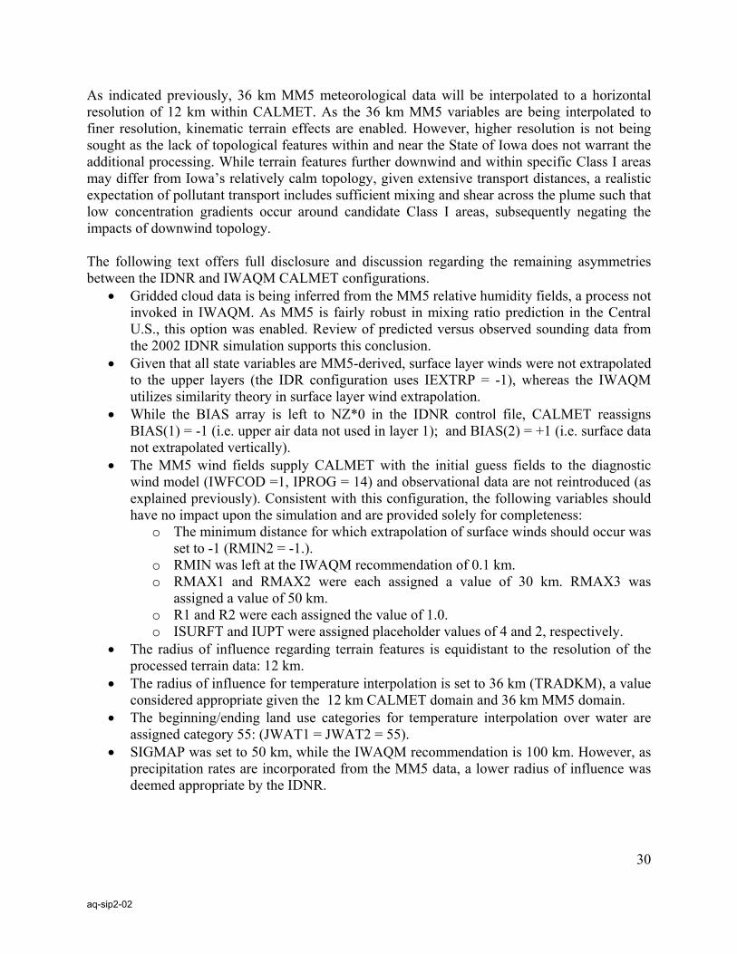
As indicated previously, 36 km MM5 meteorological data will be interpolated to a horizontal resolution of 12 km within CALMET. As the 36 km MM5 variables are being interpolated to finer resolution, kinematic terrain effects are enabled. However, higher resolution is not being sought as the lack of topological features within and near the State of Iowa does not warrant the additional processing. While terrain features further downwind and within specific Class I areas may differ from Iowa’s relatively calm topology, given extensive transport distances, a realistic expectation of pollutant transport includes sufficient mixing and shear across the plume such that low concentration gradients occur around candidate Class I areas, subsequently negating the impacts of downwind topology. The following text offers full disclosure and discussion regarding the remaining asymmetries between the IDNR and IWAQM CALMET configurations.

• Gridded cloud data is being inferred from the MM5 relative humidity fields, a process not invoked in IWAQM. As MM5 is fairly robust in mixing ratio prediction in the Central U.S., this option was enabled. Review of predicted versus observed sounding data from the 2002 IDNR simulation supports this conclusion.

• Given that all state variables are MM5-derived, surface layer winds were not extrapolated to the upper layers (the IDR configuration uses IEXTRP = -1), whereas the IWAQM utilizes similarity theory in surface layer wind extrapolation.

• While the BIAS array is left to NZ*0 in the IDNR control file, CALMET reassigns BIAS(1) = -1 (i.e. upper air data not used in layer 1); and BIAS(2) = +1 (i.e. surface data not extrapolated vertically).

• The MM5 wind fields supply CALMET with the initial guess fields to the diagnostic wind model (IWFCOD =1, IPROG = 14) and observational data are not reintroduced (as explained previously). Consistent with this configuration, the following variables should have no impact upon the simulation and are provided solely for completeness:

o The minimum distance for which extrapolation of surface winds should occur was set to -1 (RMIN2 = -1.).

o RMIN was left at the IWAQM recommendation of 0.1 km. o RMAX1 and RMAX2 were each assigned a value of 30 km. RMAX3 was

assigned a value of 50 km. o R1 and R2 were each assigned the value of 1.0. o ISURFT and IUPT were assigned placeholder values of 4 and 2, respectively.

• The radius of influence regarding terrain features is equidistant to the resolution of the processed terrain data: 12 km.

• The radius of influence for temperature interpolation is set to 36 km (TRADKM), a value considered appropriate given the 12 km CALMET domain and 36 km MM5 domain.

• The beginning/ending land use categories for temperature interpolation over water are assigned category 55: (JWAT1 = JWAT2 = 55).

• SIGMAP was set to 50 km, while the IWAQM recommendation is 100 km. However, as precipitation rates are incorporated from the MM5 data, a lower radius of influence was deemed appropriate by the IDNR.

aq-sip2-02

31

Appendix D Excerpt from the: North Dakota Department of Health – Division of Air Quality Protocol for BART-Related Visibility Impairment Modeling Analyses in North Dakota Draft September 2005 preference for monthly average relative humidity implies the use of CALPOST visibility Method

6 (MVISBK = 6).

In order to develop background conditions for visibility Method 6, CALPOST requires monthly

background concentrations of ammonium sulfate, ammonium nitrate, coarse particulate mass,

organic carbon, soil, and elemental carbon. Annual averages reflective of natural background

conditions for these species are found in EPA=s AGuidance for Estimating Natural Visibility

Conditions Under the Regional Haze Program@ (2003)2. For each Class I area, this guidance

document provides separate deciview values representative of annual average natural

background, and natural background for the 20 percent best days.

The EPA natural visibility guidance document does not provide speciated background

concentrations (above) representative of the 20 percent best days, as would be needed for

implementation of CALPOST Method 6 consistent with the BART rule. Upon consultation with

EPA and National Park Service/Fish and Wildlife Service representatives3, it was concluded that

the annual concentrations (Table 2-1 in guidance document) should be scaled back, in equal

2EPA, 2003. Guidance for Estimating Natural Visibility Conditions Under the Regional Haze

Program. Office of Air Quality Planning and Standards, Research Triangle Park, NC 27711.

3NDDH, 2005. Electronic message summarizing BART modeling-related conference-call discussion with representatives of EPA, National Park Service, and Fish and Wildlife Service, August 31, 2005

aq-sip2-02

32

proportion, until they converge to lower concentratons that produce the deciview value specified

for the 20 percent best days (guidance document Appendix B) to provide the necessary

CALPOST input. The scaling procedure would be conducted separately for each Class I area.

The scaling procedure as applied by NDDH is illustrated here for Theodore Roosevelt National

Park (TRNP). From Appendix B in the natural visibility guidance document, the deciview value

for annual average natural conditions at TRNP is 4.75, and the deciview value for the 20 percent

best days is 2.19. Note that the TRNP annual average deciview value reflects natural

background components for the US west region. To obtain the speciated background

concentrations representative of the 20 percent best days at TRNP, the deciview value (2.19)

must first be converted to light extinction. The relationship between deciviews and light

extinction is expressed,

dv = 10 ln (bext/10) or

bext = 10 exp (dv/10) where

dv represents deciviews, bext represents total light extinction expressed in inverse megameters (Mm-1).

Using this relationship with a deciview value of 2.19, one obtains a light extinction value of

12.45 Mm-1. Next, the natural visibility guidance document background concentrations for

annual average (Table 2-1, west) are adjusted in order to provide the extinction value just

determined (12.45 Mm-1). The relationship between light extinction and background

concentrations is:

aq-sip2-02

33

bext = (3) f (RH) [ammonium sulfate] + (3) f (RH) [ammonium nitrate] + (0.6) [coarse mass] + (4) [organic carbon] + (1) [soil] + (10) [elemental carbon] + bray

where

bracketed quantities represent background concentrations in μg/m3, values in parenthesis represent scattering efficiencies, f (RH) is the relative humidity adjustment factor (applied to hygroscopic species only), bray is light extinction due to Rayleigh scattering (10 Mm-1 used for all Class I areas).

Substituting the annual average natural background values and TRNP f (RH) from the natural

visibility guidance document, and including the coefficient for scaling, one obtains

12.45 = (3) (2.56) [0.12] X + (3) (2.56) [0.1] X + (0.6) [3.0] X + (4) [0.47] X + (1) [0.5] X + (10) [0.02] X + 10

where

X represents scaling factor to convert annual average natural background concentrations to values representative of 20 percent best days.

Solving for X provides a value of 0.403. This scaling factor was applied to the annual average

natural background components in the natural visibility guidance document (Table 2-1, west

region) to obtain background components for the 20 percent best days for TRNP. The scaling

procedure was repeated for Lostwood Wilderness Area.

Results of the scaling procedure are shown in Table 3-6, which includes speciated natural

background concentrations representative of annual average visibility, 20 percent best days for

Theodore Roosevelt National Park, and 20 percent best days for Lostwood Wilderness Area.

aq-sip2-02

34

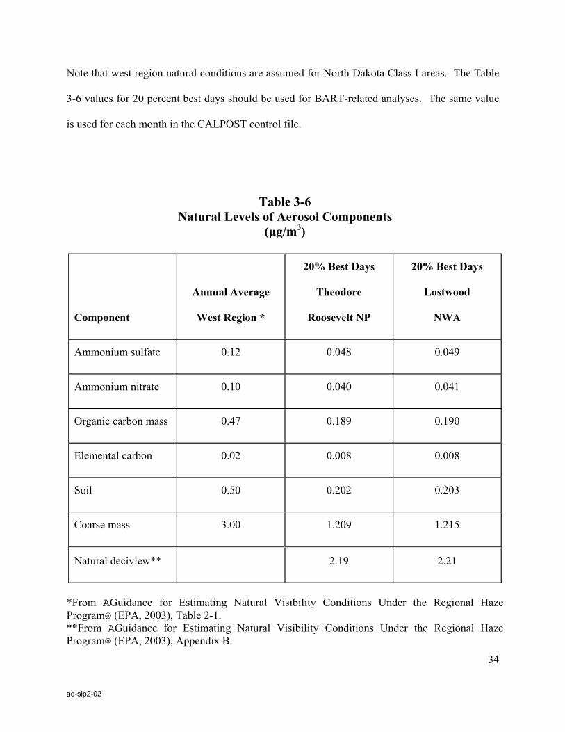
Note that west region natural conditions are assumed for North Dakota Class I areas. The Table

3-6 values for 20 percent best days should be used for BART-related analyses. The same value

is used for each month in the CALPOST control file.

Table 3-6 Natural Levels of Aerosol Components (μg/m3)

Component

Annual Average

West Region *

20% Best Days

Theodore

Roosevelt NP

20% Best Days

Lostwood

NWA

Ammonium sulfate

0.12

0.048

0.049

Ammonium nitrate

0.10

0.040

0.041

Organic carbon mass

0.47

0.189

0.190

Elemental carbon

0.02

0.008

0.008

Soil

0.50

0.202

0.203

Coarse mass

3.00

1.209

1.215

Natural deciview**

2.19

2.21

*From AGuidance for Estimating Natural Visibility Conditions Under the Regional Haze Program@ (EPA, 2003), Table 2-1. **From AGuidance for Estimating Natural Visibility Conditions Under the Regional Haze Program@ (EPA, 2003), Appendix B.

aq-sip2-02

35

Monthly RH adjustment factors (RHFAC input in CALPOST) for Theodore Roosevelt National

Park and Lostwood Wilderness Area BART-related analyses are provided in Table 3-7. These

values are also from the EPA guidance document for natural visibility conditions. One other

setting needed for CALPOST development of natural background is extinction due to Rayleigh

scattering (BEXTRAY), which should be left at the default value of 10.0.

Table 3-7 Monthly RH Adjustment Factors*

Month

Theodore Roosevelt NP

Lostwood NWA

Jan Feb Mar Apr May Jun

2.9 2.8 2.8 2.3 2.3 2.5

3.0 2.9 2.9 2.3 2.3 2.6

Jul Aug Sep Oct Nov Dec

2.4 2.2 2.2 2.3 3.0 3.0

2.7 2.4 2.3 2.4 3.2 3.2

* From AGuidance for Estimating Natural Visibility Conditions Under the Regional Haze

Program@ (EPA, 2003)

The remainder of CALPOST control file settings are intuitive, and mirror settings in the

CALPUFF control file. Settings as discussed above are incorporated in the CALPOST control

file developed by the NDDH for BART-related visibility analyses. A sample file with NDDH

settings will be provided upon request.

aq-sip2-02