bert ju¨ttler evolutionof t-splinelevelsetsformeshingnon

The Visual Computer manuscript No.(will be inserted by the editor)

Huaiping Yang · Bert Juttler

Evolution of T-spline Level Sets for Meshing Non-uniformlySampled and Incomplete Data

Abstract Given a large set of unorganized point sampledata, we propose a new framework for computing a tri-angular mesh representing an approximating piecewisesmooth surface. The data may be non–uniformly dis-tributed, noisy, and they may contain holes. This frame-work is based on the combination of two types of surfacerepresentations: triangular meshes, and T-spline level sets,which are implicit surfaces defined by refinable splinefunctions allowing T-junctions. Our method contains threemain steps. Firstly, we construct an implicit representa-tion of a smooth (C2 in our case) surface, by using anevolution process of T-spline level sets, such that theimplicit surface captures the topology and outline of theobject to be reconstructed. The initial mesh with highquality is obtained through the marching triangulationof the implicit surface. Secondly, we project each datapoint to the initial mesh, and get a scalar displacementfield. Detailed features will be captured by the displacedmesh. Finally, we present an additional evolution pro-cess, which combines data-driven velocities and feature-preserving bilateral filters, in order to reproduce sharpfeatures. We also show that various shape constraints,such as distance field constraints, range constraints andvolume constraints can be naturally added to our frame-work, which is helpful to obtain a desired reconstructionresult, especially when the given data contains noise andinaccuracies.

Keywords Mesh reconstruction · Point cloud ·Displacement maps · T-spline · Level sets

1 Introduction

We consider the problem of surface reconstruction andapproximation from unorganized data points. Due to the

H. Yang, B. JuttlerInstitute of Applied Geometry, Johannes Kepler University4040 Linz, AustriaE-mail: [email protected], [email protected]

widespread use of 3D scanning devices for shape acquisi-tion, this problem has an increasing number of applica-tions in computer graphics, computer aided design, com-puter vision and image processing. Depending on thearea of the application, the reconstructed surface mayhave a explicit representation (e.g. meshes) or an im-plicit representation (e.g. level sets). Among the variousapproaches, these two representations may complementeach other. On the one hand, the implicit representa-tions [51] offer advantages such as the non-existence ofthe parametrization problem, repairing capabilities of in-complete data and simple operations of shape editing,but they are hard to model sharp features [39]. On theother hand, the explicit representations can easily han-dle sharp features, but have difficulties when processingtopology changes.

1.1 Our Work

We propose a hybrid model for surface reconstruction bycombining two types of representations: an implicit T-spline level set and a mesh. Given a set of unorganizedand noisy data points without normals as input, we wantto reconstruct a mesh surface which approximates thedata. We develop a three-phase algorithm (cf. Fig. 1) toperform this reconstruction:

1. Initial mesh generation (Fig. 1 (c)). In the first phase,we use an evolution process (Fig. 1 (a) and (b)) tocreate an implicit representation, which is defined asthe zero level set of a C2 T-spline scalar function. Theobtained T-spline level set (with correct topology) isto serve as a smooth base surface S0 for the displace-ment mapping. A high-quality initial mesh (with ac-curate normals) is generated from the implicit func-tion by using the marching triangulation [26] method.

2. Displacement mapping (Fig. 1 (d)). In the secondphase, we produce a smooth scalar displacement field,which is computed by projecting data points to theinitial mesh. Small geometric features are then con-structed by the displacement mapping of the mesh

2 Huaiping Yang, Bert Juttler

(a) (b) (c) (d) (e)

Fig. 1 Mesh reconstruction of the Rocker-Arm model. The figure shows the data points and the T-mesh in (a), an interme-diate T-spline level set during the evolution in (b), the final T-spline level set (the initial mesh) in (c), the displaced meshin (d), and the final mesh with sharp features in (e).

along the normal direction, which is guided by thesmooth gradient vector field of the implicit function.

3. Recovering sharp features (Fig. 1 (e)). In the thirdphase, we use an additional evolution process, whichcombines data-driven velocities and feature-preservingbilateral filters, in order to better represent sharp fea-tures.

This paper is an extension to our work [55] presentedat Shape Modeling International 2007. In this extendedversion, we concentrate more on the process generatingthe base surface, i.e., we show how to formulate the evo-lution of T-spline level sets. More specifically, we dis-cuss how to combine different shape constraints, suchas distance field constraints, range constraints and vol-ume constraints, into the framework such that a morerobust and effective evolution process can be establishedthat produces the desired result. The distance field con-straints help us to avoid additional branches and singu-larities of the level sets, without having to use costlyre-initialization steps. The range constraints allow usto specify regions lying inside or outside of the recon-structed surface. A suitable volume constraint can beused to stop the level sets from entering the holes in thedata. We note that these constraints have been used inour previous work [18] in 2D for dual evolution of planarB-spline curves and T-spline level sets.

Our method combines two types of representations:the implicit T-spline level set and the mesh. This com-bination strategy makes our method benefit from theadvantages of both representations. On the one hand,the evolution of T-spline level sets is able to capture thecomplex topology of noisy data. On the other hand, themesh representation helps to produce detailed and sharpfeatures. Compared with other existing approaches forsimilar purposes, our method also shows the followingadvantages:

1) The use of two complementary representations canimprove and speed up some geometric computations in

the algorithm. For example, with the help of implicit rep-resentation, a high-quality initial mesh can be obtained,and the projection of the data points to the base surfacecan be efficiently computed by Newton iteration.

2) We use an evolution process to recover the sharpfeatures. The evolution is governed by a combination oftwo terms: a data-driven velocity and a bilateral filtering.This evolution process can produce sharp features, whichare faithful to the given data.

3) By incorporating the range constraints and volumeconstraints, we are able to conveniently exploit the a pri-ori knowledge about the geometric properties of the ob-ject to be reconstructed. This is especially helpful whenthe given data contains noise and inaccuracies.

1.2 Related Work

Numerous approaches have been proposed to computea surface approximation of a given set of unorganizedpoints. Depending on the area of the application, differ-ent representations have been used, such as triangularmeshes [3,7,15,38,2,41,47], subdivision surfaces [28,44,12], parametric spline surfaces [16,23], discretized levelsets [42,57,8], scalar spline functions [45,33], radial basisfunctions [10,40] and point set surfaces [1,43,19]. It is be-yond the scope of this paper to give a detailed overviewof all the existing work. [29] gives an excellent surveyof the previous work on surface extraction from pointclouds.

In this paper, we suggest a new reconstruction algo-rithm combining two types of representations: an implicitT-spline level set and a mesh. The proposed method re-lies on two main tools: displacement mapping [14] andbilateral filtering [48,50]. In the remainder of this sec-tion, we will describe some related work about these twotools.

Evolution of T-spline Level Sets for Meshing Non-uniformly Sampled and Incomplete Data 3

Given a smooth base surface S0, a displaced surface Scan be generated by a scalar field (a displacement map),which specifies the displacement values along the normaldirections of S0. The use of displacement maps is quitepopular for geometric modeling purposes. They are usedin high end rendering systems [14,5], to capture the finedetail of a 3D photography model [36], for geometric sim-plification with appearance-preserving [13], for buildingsemi-regular multiresolution meshes from an arbitraryconnectivity input mesh[25] and for multiresolution meshdeformations [35]. In order to avoid cracks between ad-jacent triangles of a mesh, the interpolated normal isused [24] to displace the surface, B-spline surfaces arefitted [36] to the mesh before the displacement mapping,displaced subdivision surfaces [37] are suggested which isbased on the butterfly subdivision scheme. There are alsoexisting approaches for reconstructing a displaced sub-division surface directly from a given set of points [31].Most recently, the author in [56] presents a displacedsurface representation based on a manifold structure.

Extracting sharp features from 3D data is impor-tant [49], but difficult due to the feature-insensitive sam-pling and the noise of the given data. Many approacheshave been proposed to address this problem [27,30,53,6]. As a non-iterative scheme for edge-preserving smooth-ing, the bilateral filter is used in [20] and [32] to denoisea given surface. The author in [52] presents a robust gen-eral approach conducting bilateral filters to govern thesharping of triangular meshes. Also, the authors in [4]conduct the bilateral filter in the reconstruction of sur-faces from scattered data.

The remainder of the paper is organized as follows.The next section describes how to formulate the evo-lution process of T-spline level sets, in order to gener-ate the smooth base surface for the object reconstruc-tion. Section 3 discusses the combination of differentconstraints into the evolution process. In particular, itis shown how to incorporate distance field constraints,range constraints and volume constraints such that theT-spline level sets evolution will be more robust and ef-fective when dealing with non-uniformly sampled andincomplete data. Section 4 presents how to reconstructgeometric details and sharp features of the object by de-riving a mesh representation from the smooth implicitsurface. After presenting some experimental results inSection 5, we conclude this paper and discuss futurework.

2 Evolution of T-spline Level Set for Base

Surface Generation

In this section, we describe how to generate the basesurface through the evolution of T-spline level sets. Theinput of our algorithm is a set of unorganized (maybenoisy and defected) data points (pk)k=1,2,...,n, which arescattered over an unknown piecewise smooth surface Sp.

The base surface represented S0 by T-spline level setswill capture the topology and the outline of the surfaceSp.

2.1 Definition of T-spline Level Sets

The T-spline level set Γ (f) is defined as the zero set ofa trivariate T-spline function f over some domain D,

Γ (f) = { (x, y, z) ∈ D ⊂ R3 | f(x, y, z) = 0 }, (1)

where

f(x, y, z) =

∑ni=1 ciBi(x, y, z)

∑ni=1 Bi(x, y, z)

(2)

are T-spline [46] functions in 3D, with the real coeffi-cients (control points) ci, i = 1, 2, ..., n. For cubic T-splines, the basis functions are

Bi(x, y, z) = N3i0(x)N3

i0(y)N3i0(z), (3)

where N3i0(x), N3

i0(y) and N3i0(z) are certain cubic B-

splines, whose associated knot vectors are determinedby the T-spline control grids (T-mesh).

In order to simplify the notation, we use x to repre-sent the point x = (x, y, z) in 3D, and gather the controlcoefficients (in a suitable ordering) in a column vector c.The T-spline basis functions form another column vectorb = [b1, b2, ..., bn]⊤, where

bi =Bi(x)

∑ni=1 Bi(x)

, i = 1, 2, ..., n.

Now the T-spline function f(x) = b(x)⊤c.T-splines [46] are generalizations of tensor product B-

splines. T-spline control grids permit T-junctions, whichprovides a valuable property of local refinement. As shownin Figure 2, much less (decreased by 71%) control pointsare needed to represent the same level set (a horse) bytrivariate T-splines than that by trivariate tensor prod-uct B-splines. Since a T-spline function is piecewise ra-tional, the T-spline level sets are piecewise algebraic sur-faces (C2 in our case).

The T-spline control grid (T-mesh) (cf. Fig. 1 (a)) isconstructed through octree subdivision of the functiondomain D, as follows.

1. Set the initial T-mesh to be an axis-aligned boundingbox of the cubic domain which contains all the datapoints.

2. For each cell containing more than n0 data points(n0 is a user-specified constant value), subdivide itby applying the octree subdivision.

3. Repeat step 2 until a user-specified threshold (e.g., amaximum level of subdivision) is reached or no cellcontains more than n0 data points any more.

In this way, the distribution of T-spline control points ismade adaptive to the geometry of the object to be recon-structed, which usually leads to a sparse representation.


(a) B-splines with 5148 control points (b) T-splines with 1484 control points

Fig. 2 A horse implicitly defined by trivariate B-spline (T-spline) scalar functions.

2.2 Evolution of T-spline level sets

Consider a T-spline level set Γ (f) defined as the zero setof a time-dependent function f(x, τ), where

f(x, τ) = b(x)⊤c(τ), (4)

with some time parameter τ . It will be subject to theevolution process

∂x

∂τ· n(x, τ) = v(x, τ) · n(x, τ), x ∈ Γ (f), (5)

which is driven by a (possibly time-dependent) vectorfield v. Note that we only consider the normal compo-nent (v · n) of the velocity along the level set, since thetangent velocity does not change the shape at all. Theunit normal vector n is given by

n(x, τ) =∇f(x, τ)

|∇f(x, τ)|. (6)

During the evolution, the definition of T-spline levelsets

f(x, τ) ≡ 0, x ∈ Γ (f), (7)

implies

∂f(x, τ)

∂τ+ ∇f(x, τ) ·

∂x

∂τ= 0, x ∈ Γ (f). (8)

Combining (5), (6) and (8), we get the evolution equationof T-spline level sets under the vector field v,

∂f(x, τ)

∂τ= −v(x, τ) · ∇f(x, τ), x ∈ Γ (f). (9)

In our method, we always start the evolution of T-spline level sets from an initial level set, which containsall data points inside. The initial level set function f canbe found by approximating it to the signed distance fieldof a bounding sphere or a rough offset of the surface tobe reconstructed [57].

2.3 Evolution Speed Function

The speed function v plays a a key role in the evolutionof T-spline level sets. In order to capture the base surfaceof the given data points, we use a similar speed functionas that proposed by Caselles et al. [11],

v = e(d)(γ + κ)n − (1 − e(d))(∇d · n)n (10)

where γ is a constant velocity (which is also known as aballoon force), κ = div(∇f/|∇f |) is the mean curvatureof the level set surface, d is the unsigned distance func-

tion of the data points, and e(d) = 1− e−ηd2

is the edgedetector function. η is pre-defined, and its value is af-fected by the size of the data range. In our experimentalsetting, all data points are contained in a unit boundingbox (−1 ≤ x, y, z ≤ 1), and we usually set η = 1.

The speed function (10) is a linear combination oftwo parts. In the first part, the mean curvature termκ makes the level set smooth, and the balloon force γ isused to increase the speed of the evolution (especially forcapturing narrow concave boundaries). The second partattracts the level set to the detected boundary edges.The edge detector function e(d) is used as weighting co-efficients to balance the influence of the two parts.

2.4 Discretization of the Evolution Equation

The evolution equation (9) under the speed function (10)is discretized by uniformly sampling a set of points xj ,j = 1, . . . , N0 on the T-spline level set. We use themarching triangulation method to generate the uniformsamples, which will be described later in Section 4.1.Since usually the number of sample points N0 is muchlarger than the number of T-spline control coefficientsn, the equation can not be exactly satisfied. We use aleast-squares approach to choose the time derivative of


the function f by solving

E =

N0∑

j=1

( f(xj , τ) + v(xj , τ) · ∇f(xj , τ) )2 → Min (11)

where f(xj , τ) = ∂f(xj , τ)/∂τ is the time derivative of f .In order to prevent the problem from being ill-posed,

we add a regularization term to the above function E tobe minimized,

E + λc|c|2 → Min, (12)

where c is the time derivative of the T-spline controlcoefficients, and λc is a pre-scribed small constant [17].

Since in our case f(x, τ) = b(x)⊤c(τ) (cf. Equa-tion (4)), the solution to (12) can be found by solvinga sparse linear system of equations.

Then we generate the updated control coefficients

c(τ + ∆τ) = c(τ) + c∆τ. (13)

by using an explicit Euler step ∆τ . ∆τ is chosen as

∆τ = min(1, {h

|v(xj , τ) · n(xj , τ)|}0≤j≤N0

) (14)

where h is a user-defined constant to indicate the max-imum allowed evolution step size for each sample pointon the T-spline level set.

3 Constraints for T-spline level sets evolution

In this section, we present three different constraints in-cluding distance field constraints, range constraints, andvolume constraints, which can be applied to improve therobustness and effectiveness of T-spline level sets evolu-tion.

3.1 Distance Field Constraint

The distance field constraint is used to restore the signed

distance property of the T-spline level set function duringthe evolution, without having to use the costly level set

reinitialization procedure [54].Since an ideal signed distance function φ satisfies

|∇φ| = 1 everywhere in the domain of D, we proposethe following constraint term

S0 =

∫

D

(∂|∇f(x, τ)|

∂τ+|∇f(x, τ)|−1 )2dV → Min, (15)

where dV is the volume element. This constraint acts asa penalty function to penalize the deviation of f from asigned distance function.

In practice, we realize that it is usually sufficient tomaintain the signed distance property of f only in a smallneighborhood of the zero level set (like the narrow-band

(a) (b) (c)

Fig. 3 The distance field constraint (DFC) for T-spline levelsets in 2D. The figure shows the data points with T-mesh in(a), the resulting level set function without DFC in (b), andthe resulting level set function with DFC in (c).

level set method). Thus we propose to use a much moreefficient version of the distance field constraint,

S =

N0∑

j=1

(∂|∇f(xj , τ)|

∂τ+ |∇f(xj , τ)| − 1)2, (16)

by only considering the sample points xj , j = 1, . . . , N0

on the zero level set. Combining the distance field con-straint into the evolution equation, we get the new ob-jective function to be minimized

E + λc|c|2 + λsS → Min. (17)

We usually choose the weight λs = 0.1 in our experi-ments. More details about the influence and choice of λs

are described in [54].Fig. 3 illustrates an example of using the distance

field constraint. As shown in (b), without the using ofdistance field constraints, the level set function becomesvery steep (or flat) in some regions, which may causedifficulties in maintaining the numerical stability duringthe evolution. This situation can be cured by applyingthe distance field constraint, as shown in (c).

3.2 Range Constraint

One typical advantage of the implicit representation of asurface is fast inside/outside distinction. In our case, weassume that the T-spline level set function f(x) > 0 rep-resents the region outside the surface, and f(x) < 0 in-side the surface. The range constraints are used to spec-ify regions which should lie inside/outside the surface tobe reconstructed. More specifically, we consider a set ofpoints {xk}k=1,...,N1

which should not lie outside the zerolevel set, and another set of points {yk}k=1,...,N2

whichshould not lie inside the zero level set,

{

f(xk) ≤ 0, k = 1, . . . , N1.f(yk) ≥ 0, k = 1, . . . , N2.

(18)

The above range constraints can be achieved by addingcorresponding penalty terms to the objective function (17)

such that the time derivative satisfies f(xk) < 0 if f(xk) >


0, and f(yk) > 0 if f(yk) < 0, respectively. For example,to the first set of points xk, we propose to use

R =

N1∑

k=1

(f(xk, τ) − f(xk, τ))2α(f(xk, τ)) (19)

where the ’activator’ function α is defined as

α(f) =

{

1, f > 0.0, f ≤ 0.

(20)

The second set of points yk can be dealt with similarly.The range constraints are very useful in practical ap-

plications. As noticed in [22], the presence of the bal-loon force in the evolution speed function (10) may leadto problems when a large time step size is used for theevolution, because the level set may skip over and missobject boundaries defined by incomplete data. This prob-lem can be handled by treating all the data points as theset of points xk to be constrained not outside the surface,which is easily done by combining the range constraintterm (19) into the objective function to be minimized

E + λc|c|2 + λsS + λrR → Min. (21)

Usually we use a large value for the weight λr (e.g.λr = 100) of the range constraint. Figure 4(b) and (c) il-lustrate different results before and after applying rangeconstraints. Another example is given in Figure 6.

3.3 Volume Constraint

In some applications of surface reconstruction, the vol-ume of the object to be reconstructed may be knowna priori. In order to utilize this geometric information,we propose to formulate the volume constraint for theevolution of surfaces.

Let V0 be the volume of the initial surface (T-splinelevel set), and V∞ be the volume of the final surface. Inour case V0 > V∞, since the initial surface contains thefinal surface. By defining a smooth monotonic functionV (τ) with respect to the time τ such that V (0) = V0 andV (τ) → V∞ as τ → ∞, the volume of the surface willcontinuously converge to the desired value V∞. Then thevolume constraint is represented as

∫

Γ

vn(x, τ)dA = V (τ), (22)

where A is the area element of the level set surface Γ ,and

vn(x, τ) = −f(x, τ)

|∇f(x, τ)|(23)

is the normal velocity of the T-spline level set. We usethe exponential function to define the curve of volumechanges

V (τ) = (V0 − V∞)e−τ + V∞, (24)

(a) (b)

(c) (d)

Fig. 4 The range constraint and volume constraint. The fig-ure shows the data points with T-mesh in (a), the resultingT-spline level set without range and volume constraints in(b), the result with range constraint in (c), and the resultwith volume constraint in (d).

Fig. 5 The volume function V (τ ).

which is illustrated in Fig. 5. It becomes a volume pre-serving constraint when V∞ = V0.

By combining (22) and (23), the volume constraintis linear in the time derivatives of the T-spline controlcoefficients. Now the evolution of T-spline level sets istransformed into a least-squares problem (21) subject tothe linear volume constraint. By using the method ofLagrange multipliers, the solution can be obtained bysolving a sparse linear system of equations.

The volume constraint is very helpful to handle in-complete data with large holes. Without the volume con-straint, the level set may easily shrink into the holesduring the evolution (cf. Fig. 4(b) and (c)). With thevolume constraint, the level set surface will keep an ap-


propriate volume and the holes will be properly closed(cf. Fig. 4(d)).

4 Mesh Reconstruction with Geometric Details

and Sharp Features

4.1 Initial Mesh Generation through MarchingTriangulation

After the smooth base surface S0 is obtained, we usethe Marching Triangulation [26] method to generate themesh representation of S0. We choose the Marching Tri-angulation since it is able to produce a high-quality tri-angular mesh. Other polygonization methods [34,21] canbe also considered.

The requirement for applying the Marching Triangu-lation method is that the function value f(x) and thegradient ∇f(x) are available for any point x in the func-tion domain. This is satisfied by our T-spline function fsince f is C2 continuous in the domain of interest.

A key procedure of the Marching Triangulation isthe choice of seed points on the implicit surface. If theimplicit surface contains multiple components, then atleast one seed point must be chosen for one component,otherwise those components without seed points will notbe triangulated. In our case, since the implicit functionf defines a good base surface S0 for the data points(pk)k=1,2,...,n, we solve this problem as follows:

1. Project each data point (pk)k=1,2,...,n to S0, get thecorresponding closest point (qk)k=1,2,...,n. (More de-tails will be described later in Section 4.2.1.)

2. Initialize the set of potential seed pointsP = {pk}k=1,2,...,n.

3. Initialize the set of generated triangles M = ∅.4. Choose an arbitrary seed point si from P , and apply

the Marching Triangulation to get a new mesh Mi.Add Mi to M.

5. For each potential seed point (pk)pk∈P , compute thedistance from its closest point qk to the new meshMi. If the distance is sufficiently small, then remove(pk) from P .

6. Repeat steps 4 ∼ 5 until P = ∅.7. Output the generated triangular meshes M.

A similar strategy is also used to generate uniformsamples on the T-spline level set during the evolution.The idea is to treat the sample points on the currentsurface as the data points in the above procedure whenapplying the marching triangulation for the next surface.Since the triangulation of the initial surface with onlyone component is easily obtained, all the other surfacescan be handled subsequently.

The Marching Triangulation method is very fast andalso simple to implement. As shown in Section 5, usu-ally we can generate over 10, 000 triangles within sec-onds. The generated mesh is semi-regular, and the vast

majority of the mesh vertices have valence 6. The edgelength of the triangles is approximately indicated by themarching step length δt, which can be determined bythe feature size of the reconstructed surface. We usuallychoose δt = 0.2lT , where lT is the diameter of the cellsat the finest level of the T-mesh.

4.2 Displacement Mapping

After the base surface S0 is triangulated by the initialmesh M0, the topology and parametrization of the sur-face to be reconstructed is now defined by M0. Fine geo-metric details are to be captured through a displacementmapping,

M = M0 + D, (25)

where the displacement field D is generated from thedata points (pk)k=1,2,...,n.

4.2.1 Data Points Projection

In order to get the displacement field D, we project alldata points to the initial mesh M0. Since M0 is a dis-cretization of the smooth base surface S0, the projectionprocess can be transformed into the computation of clos-est points on the surface S0, which is implicitly definedby the T-spline function f . Thus, for each data pointpk, one can compute its closest point qk efficiently byNewton iteration. Then we associate qk to its closesttriangle Tk, which will be needed later for the Gaussianfiltering of the displacement field. The whole projectionprocedure is given as follows:

1. For each triangle Ti ∈ M0, initialize the array of in-dices of its associated data points Ii = ∅.

2. Initialize the displacement array (dk = 0)k=1,2,...,n.3. For each data point (pk)k=1,2,...,n,

(a) Initialize the closest point qk,0 = pk.(b) Using Newton’s method to get the updated closest

point qk,i+1 = qk,i −f(qk,i)

‖∇f(qk,i)‖2∇f(qk,i).

(c) Repeat step 3.2 until ‖qk,i+1−qk,i‖ is sufficientlysmall. Set qk = qk,i+1.

(d) Set the signed displacement value dk = sign(f(pk))·‖pk − qk‖.

(e) Find the closest vertex vkvof M0 to the point qk.

(f) From the one-ring neighborhood of vkv, get the

closest triangle(s) Tktto qk.

(g) Add k to the array of indices Ikt.

4. Output (Ii)Ti∈M0and the displacement array (dk)k=1,2,...,n.

Please note that we do not compute any ray-triangleintersections for the data points projection. This im-provement of efficiency has been achieved by exploitingthe advantages of the implicit representation of the basesurface.


4.2.2 Displaced Mesh

After the scalar displacement field D is already sampledat each closest point (qk)k=1,2,...,n, we then want to mapit to each vertex v of the initial mesh M0,

v = v + d(v) · n. (26)

Note that the normals n are computed from the implic-itly defined T-spline surface, n = ∇f

‖∇f‖ |v, instead of the

discretized mesh.Since the given data points are often noisy, the sam-

pled field is therefore not smooth. In order to avoid cracksbetween adjacent triangles of the displaced mesh, we useGaussian filtering to smooth the displacement field (weusually choose σ = 2δt, where δt is the marching steplength in Section 4.1). Of course, the use of Gaussian fil-tering will also smooth some desired sharp features. Thenext section will describe how to recover these sharp fea-tures.

After the displacement mapping, the quality of thedisplaced mesh may be degraded. In the worst case, flipsor self-intersections may happen to the displaced trian-gles, where the displacement values are too large for somedeep convex or concave parts of the object surface. Theallowed displacement can be bounded with the help ofthe principal curvature radii, which can be estimatedfrom the implicit T-spline function.

One way to prevent this problem is to find a betterbase surface by using more degrees of freedom (T-splinecontrol coefficients) and applying the ’final refinement’step [54] to make the T-spline level set more close tothe data points. In our algorithm, we use the principalcurvature radii as an indicator. If the displacement valueis close to or larger than the corresponding curvatureradii, we check if the displaced triangle is flipped. If someflips happen, we refine the T-spline level set to make surethat the displacement mapping is intersection free.

4.3 Recovering Sharp Features

After the displacement mapping, the displaced mesh ap-proximates the data points far better than the initialmesh. Most parts of the object to be reconstructed are al-ready well fitted, except near sharp features. In this sec-tion, we introduce a data-driven bilateral filtering methodto reproduce sharp features of the reconstructed mesh.

4.3.1 Bilateral Filter

The bilateral filter, which was originally proposed in im-age processing [48,50], is a nonlinear filter derived fromGaussian blur, with a feature-preserving term that de-creases the weights of pixels as a function of intensitydifferences. Following the formulation in [48], the bilat-eral filtering for image I(p) at the pixel p∗ is defined

as

ˆI(p∗)=∑

pj∈N(p∗)

Wc(‖p∗ − pj‖)Ws(|I(p∗) − I(pj)|)

WI(pj),

(27)

where N(p∗) is the neighborhood of p. Wc is the stan-

dard Gaussian filter with parameter σc: Wc(x) = e−x2/2σ2

c ,and Ws is a similarity weight function for feature-preserving

with parameter σs: Ws(x) = e−x2/2σ2

s . W is a normal-ization factor

W =∑

pj∈N(p∗)

Wc(‖p∗ − pj‖)Ws(‖I(p∗) − I(pj)‖).

Recently, the bilateral filter has been applied to meshdenoising while preserving sharp features [20,32]. Theauthor in [52] uses the bilateral filtering for recovering ofsharp edges on feature-insensitive sampled edges. In [4],the bilateral filter in used for data denoising such that thefiltered data points can be later connected into a meshstructure. Unlike these previous works, we combine thebilateral filtering term into a data-driven evolution pro-cess, such that the produced sharp features are faithfulto the given data points.

4.3.2 Data-Driven Bilateral Evolution

Recall that our bilateral evolution is to obtain a meshthat meets two goals:

1. It provides a good fit to the point set (pk)k=1,2,...,n.2. It recovers sharp features by conducting bilateral fil-

ters.

Consider a mesh M with time-dependent vertices V(τ) =(vi(τ))i=1,2,...,m (m is the number of vertices), whoseevolution process is governed by minimizing the followingenergy function

F (V(τ)) = Edist(V(τ)) + ωEbila(V(τ)) → min, (28)

where the two terms Edist and Ebila correspond to thetwo goals listed above, and ω > 0 is a constant weightingcoefficient.

The distance energy Edist is defined as

Edist(V(τ)) =n

∑

k=1

(qk + qk − pk)2, (29)

where qk on the mesh is the closest point of pk, and itstime derivative qk = ∂qk/∂τ can be represented as alinear combination of related vertex velocities vj

qk =∑

vj∈φ(pk)

λj vj , (30)

where φ(pk) contains 3 vertices of the corresponding tri-angle, and λj are the barycentric coordinates of qk.


eavr (10−3) emax (10−3) Run time (s)Dataset np nt nv MI MD MS MI MD MS TL MT D-Map B-EvlRocker-Arm 10044 992 8577 4.34 0.88 0.69 24.44 14.12 11.30 10.50 2.19 0.52 6.64Horse 48485 1484 9137 5.63 0.36 – 43.78 7.69 – 36.13 2.40 3.11 –Fandisk(cut) 5817 1019 12856 18.27 1.27 0.21 68.86 19.90 7.93 12.30 2.94 0.39 7.78Ball-joint 137062 988 11831 33.42 0.83 – 60.33 8.05 – 7.50 2.41 6.32 –Foot 25845 871 4517 35.86 0.62 0.55 98.47 9.07 8.22 7.94 0.81 1.19 0.63Sculpture 25386 2551 14026 3.93 0.74 0.63 20.72 6.33 5.41 56.33 5.03 1.67 6.16

Table 1 The approximation errors and the execution time of the given examples. np: number of data points; nt: numberof T-spline control points; nv: number of mesh vertices; MI : initial mesh; MD: displaced mesh; MS: sharpened mesh afterbilateral evolution; TL: T-spline level set evolution; MT: marching triangulation; D-Map: displacement mapping; B-Evl:bilateral evolution. The right three columns show the run time for the T-spline level set evolution, the marching triangulation,the displacement mapping and the bilateral evolution, respectively. The left several columns show the number of data points,the number of T-spline control points, and the number of mesh vertices. The middle columns give both the approximationerrors (eavr) and the maximum errors (emax) for the initial meshes, the displaced meshes and the final meshes, respectively.

The bilateral energy Ebila is defined as

Ebila(V(τ)) =

m∑

i=1

(vi + vi − v′i)

2, (31)

where v′i is the updated position of vi according to the

bilateral filter [52]

v′ =∑

Tj∈N(v)

Wc(‖v− cj‖)Ws(‖v − v∗j‖)

Wαjv

∗j , (32)

where v is any vertex of the mesh M , v∗j is the projec-

tion point of v on the plane of the triangle Tj , αj is thearea of Tj , cj is the center of Tj , and N(v) is the setof neighboring triangles contributing to the position ofv. Wc and Ws are the Gaussian filters as used in (27).See [52] for more details.

Combining (28), (29), (30) and (31), the minimizerof (28) leads to a quadratic objective function of the un-

known time derivatives V = (vi)i=1,2,...,m. The solution

V is found by solving a sparse linear system of equations,∇F = 0. Using explicit Euler steps vi → vi+∆τ vi, witha suitable step-size ∆τ , one can trace the evolving mesh.

Actually, in practice, we do not need to update allvertices during the data-driven bilateral evolution, sincethe non-sharp region of the surface is already well fittedby the displacement mapping. Instead, we only need toupdate those sharp-vertices with both a high dihedral an-gle and a large approximation error, while keeping v = 0for the remaining vertices. Here, we use the same methodas indicated in [52] to detect potential sharp vertices witha high dihedral angle. If the one-ring neighborhood re-gion of a potential sharp vertex is already well fitted (theapproximation error is small), then we discard it from thelist of real sharp vertices. After that, to construct Edist

and Ebila, we only consider those terms related with realsharp-vertices, such that the size of the linear system isgreatly reduced.

The bilateral evolution continues until the approxi-mation error can not be reduced any more. In our method,

the approximation error eavr is measured as the averagedistance of the data points to the mesh

eavr =1

n

n∑

k=1

‖qk − pk‖. (33)

4.3.3 Discussion

The parameters σc and σs of the bilateral filter are im-portant to get a satisfying reconstruction result. On theone hand, if σc and σs are set too large, the sharp fea-tures will be smoothed. On the other hand, if they are settoo small, the reconstruction result will be very sensitiveto the noise of the given data set. In our experimen-tal settings, we usually choose σs = σc = 2δt (δt is themarching step length in Section 4.1).

Usually within 10 iterations, the sharp features canbe well reconstructed. But because most sharp-verticesare attracted towards their corresponding sharp edges,many degenerate triangles will be produced afterwards.Therefore, in order to improve the regularity of the re-constructed mesh, a MeshSlicing [9] operation is used toremove degenerate triangles after the bilateral evolutionstops (See Figures 7 (d1), 8 (c1) and 10 (d1)).

5 Experimental results

In this section, we present some examples to demon-strate the effectiveness of our method. All the given datapoints are normalized to be contained in a cubic domain([−1, 1] × [−1, 1] × [−1, 1]). The maximum error emax

mentioned below is the maximum distance of the datapoints to the mesh. The average error eavr is the approx-imation error defined by Eq. (33). All the experimentsare run on a PC with AMD Opteron(tm) 2.20GHz CPUand 3.25G RAM. The approximation errors and the ex-ecution time are reported in Table 1.

Example 1. The first example is the Rocker-Arm model,which contains non-uniform samples with holes and sharp


(a) (b) (c)

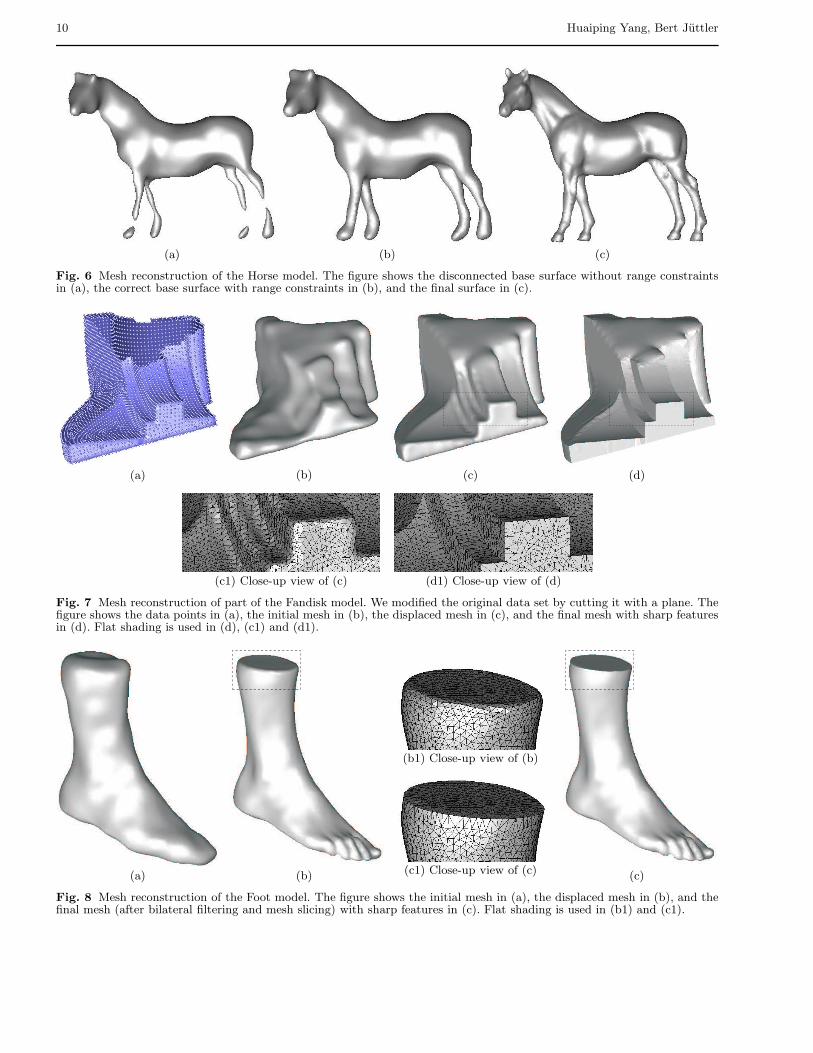
Fig. 6 Mesh reconstruction of the Horse model. The figure shows the disconnected base surface without range constraintsin (a), the correct base surface with range constraints in (b), and the final surface in (c).

(a) (b) (c) (d)

(c1) Close-up view of (c) (d1) Close-up view of (d)

Fig. 7 Mesh reconstruction of part of the Fandisk model. We modified the original data set by cutting it with a plane. Thefigure shows the data points in (a), the initial mesh in (b), the displaced mesh in (c), and the final mesh with sharp featuresin (d). Flat shading is used in (d), (c1) and (d1).

(a) (b)

(b1) Close-up view of (b)

(c1) Close-up view of (c) (c)

Fig. 8 Mesh reconstruction of the Foot model. The figure shows the initial mesh in (a), the displaced mesh in (b), and thefinal mesh (after bilateral filtering and mesh slicing) with sharp features in (c). Flat shading is used in (b1) and (c1).


(a) (b) (c)

Fig. 9 Mesh reconstruction of the Ball-joint model. The figure shows the data points and the T-mesh in (a), the initialmesh in (b), and the displaced mesh in (c).

(a) (b) (c) (d)

(c1) Close-up view of (c) (d1) Close-up view of (d)

Fig. 10 Mesh reconstruction of the Sculpture model. The figure shows the data points and the T-mesh in (a), the initialmesh in (b), the displaced mesh in (c), and the final mesh with sharp features in (d). Flat shading is used in (c1) and (d1).

features, as shown in Fig. 1. The T-spline level set adaptsits topology from genus-0 in (b) to genus-1 in (c), wherethe initial mesh is constructed. The displaced mesh isshown in (d). By using the data-driven bilateral evolu-tion, the approximation error is further reduced by 21.6%(cf. Table 1), and the sharp edges are recovered in (e).

Example 2. The second example is a horse model, asshown in Fig. 6. The narrow and thin legs of the horsecan easily split into several disconnected components in(a) without using the range constraint. After combiningthe range constraint (cf. Section 3.2), the base surfaceis correctly constructed in (b), and the final mesh withgeometric details is shown in (c).

Example 3. The third example is part of the Fandiskmodel, which was cut by a plane, creating a large hole inthe data set, as shown in Fig. 7. By using our method,the cutting hole can be filled by the T-spline level setrepresentation, and the sharp edges can be recovered bythe bilateral evolution of the mesh, as shown in (d). Theapproximation error is reduced by 83.5%, and the maxi-mum error is reduced by 60.2% during the bilateral evo-lution (cf. Table 1).

Example 4. The fourth example is the Ball-joint model,as shown in Fig. 9. Since the data points are already wellapproximated by the displacement mesh, the last phaseof our algorithm (recovering sharp features) is discarded.


Example 5. The fifth example is the Foot model, as shownin Fig. 8. After the displacement mapping in (b), thesharp edges can be recovered by the data-driven bilat-eral evolution, as shown in (c).

Example 6. The last example is a complex sculpturemodel, as shown in Fig. 10. Through the evolution ofT-spline level sets, the base surface with a correct topol-ogy is obtained in (b). The updated mesh after displace-ment mapping is given in (c). Finally, the sharp edgesare produced in (d) by using the bilateral evolution.

6 Conclusions

We have introduced a new framework for surface re-construction from unorganized data points. We use thedisplacement mapping of a smooth base surface, whichis implicitly represented by scalar T-spline functions.We have shown that, with the help of different shapeconstraints, even non-uniformly sampled and incompletedata can be handled by the implicitly defined base sur-face. Geometric details can efficiently be dealt with withthe help of the displacement mapping. The sharp fea-tures of the mesh surface are produced by using a data-driven bilateral evolution. Possible future work includescomparing results by using different forms of functionsfor the implicit representation of the base surface, andexploiting other kinds of a priori knowledge about thegeometric properties of the surface to be reconstructed.

Acknowledgment. The first author was supported bya Marie Curie Incoming International Fellowship of theEuropean commission (project 022073 ISIS). The sec-ond author was supported by the Austrian Science Fundthrough the national research network on Industrial Ge-ometry (S9202). The data sets used for our experimentsare courtesy of Stanford computer graphics laboratoryand UCI (University of California, Irvine) computer graph-ics laboratory.

References

1. M. Alexa, J. Behr, D. Cohen-Or, S. Fleishman, D. Levin,and C. Silva. Point set surfaces. In Proc. VIS’01, pages21–28, 2001.

2. R. Allegre, R. Chaine, and S. Akkouche. Convection-driven dynamic surface reconstruction. In Proc. SMI’05,pages 33–42, 2005.

3. N. Amenta, S. Choi, T. K. Dey, and N. Leekha. A simplealgorithm for homeomorphic surface reconstruction. InSCG ’00: Proceedings of the sixteenth annual symposiumon Computational geometry, pages 213–222, 2000.

4. A.Miropolsky and A.Fischer. Reconstruction with 3Dgeometric bilateral filter. In 9th ACM Symposium onSolid Modeling and Applications, pages 225–231, Genoa,Italy, 2004.

5. A. Apodaca and L. Gritz. Advanced RenderMan: Cre-ating CGI for Motion Pictures. Morgan Kaufmann, SanFrancisco, CA, 1999.

6. M. Attene, B. Falcidieno, J. Rossignac, and M. Spagn-uolo. Sharpen & Bend: Recovering curved sharp edgesin triangle meshes produced by feature-insensitive sam-pling. IEEE Transactions on Visualization and Com-puter Graphics, 11(2):181–192, 2005.

7. F. Bernardini, J. Mittleman, H. Rushmeier, C. Silva, andG. Taubin. The ball-pivoting algorithm for surface re-construction. IEEE Transactions on Visualization andComputer Graphics, 5(4):349–359, 1999.

8. J. Boissonnat and F. Cazals. Smooth surface recon-struction via natural neighbour interpolation of distancefunctions. Comput. Geom. Theory Appl., 22(1):185–203,2002.

9. M. Botsch and L. Kobbelt. A robust procedure to elim-inate degenerate faces from triangle meshes. In Proc.VMV’01, pages 283–290, 2001.

10. J. C. Carr, R. K. Beatson, J. B. Cherrie, T. J. Mitchell,W. R. Fright, B. C. McCallum, and T. R. Evans. Recon-struction and representation of 3D objects with radialbasis functions. In Proc. SIGGRAPH’01, pages 67–76,2001.

11. V. Caselles, R. Kimmel, and G. Sapiro. Geodesic activecontours. Int. J. Comput. Vision, 22(1):61–79, 1997.

12. K.-S. D. Cheng, W. Wang, H. Qin, K.-Y. K. Wong,H. Yang, and Y. Liu. Fitting subdivision surfaces to un-organized point data using SDM. In Proc. PG’04, pages16–24, 2004.

13. J. Cohen, M. Olano, and D. Manocha. Appearance-preserving simplification. In Proc. SIGGRAPH’98, pages115–122, 1998.

14. R. Cook. Shade trees. In Proc. SIGGRAPH’84, pages223–231, 1984.

15. T. K. Dey and S. Goswami. Tight cocone: a water-tightsurface reconstructor. In Proc. SMI’03, pages 127–134,2003.

16. M. Eck and H. Hoppe. Automatic reconstruction of b-spline surfaces of arbitrary topological type. In Proc.SIGGRAPH’96, pages 325–334, 1996.

17. H. W. Engl, M. Hanke, and A. Neubauer. Regularizationof Inverse Problems. Kluwer, Dordrecht, 1996.

18. R. Feichtinger, M. Fuchs, B. Juttler, O. Scherzer, andH. Yang. Dual evolution of planar parametric splinecurves and T-spline level sets. Computer-Aided Design,2007, to appear.

19. S. Fleishman, D. Cohen-Or, and C. Silva. Robust movingleast-squares fitting with sharp features. ACM Trans.Graph. (Proc. SIGGRAPH’05), 24(3):544–552, 2005.

20. S. Fleishman, I. Drori, and D. Cohen-Or. Bilateral meshdenoising. ACM Trans. Graph. (Proc. SIGGRAPH’03),22(3):950–953, 2003.

21. M. Gavriliu, J. Carranza, D. Breen, and A. Barr. Fastextraction of adaptive multiresolution meshes with guar-anteed properties from volumetric data. In Proc. VIS’01,pages 295–303, 2001.

22. R. Goldenberg, R. Kimmel, E. Rivlin, and M. Rudzsky.Fast geodesic active contours. IEEE Trans. on ImageProcessing, 10:1467–1475, 2001.

23. X. Gu, Y. He, and H. Qin. Manifold splines. GraphicalModels, 68(3):23–254, 2006.

24. S. Gumhold and T. Huttner. Multiresolution renderingwith displacement mapping. In Proceedings of the ACMSIGGRAPH/EUROGRAPHICS workshop on Graphicshardware, pages 55–66, 1999.

25. I. Guskov, K. Vidimce, W. Sweldens, and P. Schroder.Normal meshes. In Proc. SIGGRAPH’00, pages 95–102,2000.

26. E. Hartmann. A marching method for the triangulationof surfaces. The Visual Computer, 14(3):95–108, 1998.

27. H. Hoppe. Progressive meshes. In Proc. SIGGRAPH’96,pages 99–108, 1996.


28. H. Hoppe, T. DeRose, T. Duchamp, M. Halstead, H. Jin,J. McDonald, J. Schweitzer, and W. Stuetzle. Piecewisesmooth surface reconstruction. In Proc. SIGGRAPH’94,pages 295–302, 1994.

29. A. Hornung and L. Kobbelt. Robust reconstruction ofwatertight 3d models from non-uniformly sampled pointclouds without normal information. In EurographicsSymposium on Geometry Processing (SGP 2006), pages41–50, 2006.

30. A. Hubeli and M. H. Gross. Multiresolution feature ex-traction from unstructured meshes. In Proc. of IEEEVisualization’01, pages 16–25, 2001.

31. W.-K. Jeong and C.-H. Kim. Direct reconstruction ofa displaced subdivision surface from unorganized points.Graphical Models, 64(2):78–93, 2002.

32. T. Jones, F. Durand, and M. Desbrun. Non-iterative,feature-preserving mesh smoothing. ACM Trans. Graph.(Proc. SIGGRAPH’03), 22(3):943–949, 2003.

33. B. Juttler and A. Felis. Least squares fitting of algebraicspline surfaces. Adv. Comput. Math., 17:135–152, 2002.

34. T. Karkanis and A. J. Stewart. Curvature-dependent tri-angulation of implicit surfaces. IEEE Computer Graphicsand Applications, 21(2):60–69, 2001.

35. L. Kobbelt, T. Bareuther, and H. P. Seidel. Multiresolu-tion shape deformations for meshes with dynamic vertexconnectivity. Computer Graphics Forum (Proc. Euro-graphics’00), 19(3):249–260, 2000.

36. V. Krishnamurthy and M. Levoy. Fitting smooth surfacesto dense polygon meshes. In Proc. SIGGRAPH’96, pages313–324, 1996.

37. A. Lee, H. Moreton, and H. Hoppe. Displaced subdivisionsurfaces. In Proc. SIGGRAPH’00, pages 85–94, 2000.

38. B. Mederos, N. Amenta, L. Velho, and L. H.de Figueiredo. Surface reconstruction for noisy pointclouds. In Symposium on Geometry Processing, pages53–62, 2005.

39. Y. Ohtake, A. Belyaev, M. Alexa, G. Turk, and H.-P. Sei-del. Multi-level partition of unity implicits. ACM Trans.Graph. (Proc. SIGGRAPH’03), 22(3):463–470, 2003.

40. Y. Ohtake, A. Belyaev, and H.-P. Seidel. 3d scattereddata approximation with adaptive compactly supportedradial basis functions. In Proc. SMI’04, pages 31–39,2004.

41. Y. Ohtake, A. Belyaev, and H.-P. Seidel. A compos-ite approach to meshing scattered data. Graph. Models,68(3):255–267, 2006.

42. S. Osher and R. Fedkiw. Level Set Methods and DynamicImplicit Surfaces. Springer Verlag, New York, 2002.

43. M. Pauly, R. Keiser, L. Kobbelt, and M. Gross. Shapemodeling with point-sampled geometry. ACM Trans.Graph. (Proc. SIGGRAPH’03), 22(3):641–650, 2003.

44. H. Qin, C. Mandal, and B. C. Vemuri. Dynamic catmull-clark subdivision surfaces. IEEE Transactions on Visu-alization and Computer Graphics, 4(3):215–229, 1998.

45. A. Raviv and G. Elber. Three dimensional freeformsculpting via zero sets of scalar trivariate functions. InProc. 5th ACM Symposium on Solid Modeling and Ap-plications, pages 246–257, 1999.

46. T. W. Sederberg, J. Zheng, A. Bakenov, and A. Nasri.T-splines and T-NURCCs. ACM Trans. Graph. (Proc.SIGGRAPH’03), 22(3):477–484, 2003.

47. A. Sharf, T. Lewiner, A. Shamir, L. Kobbelt, andD. Cohen-Or. Competing fronts for coarse–to–fine sur-face reconstruction. In Proc. Eurographics’06, pages 389–398, 2006.

48. S. M. Smith and J. M. Brady. SUSAN–a new approachto low level image processing. Int. J. Comput. Vision,23(1):45–78, 1997.

49. W. B. Thompson, J. C. Owen, H. J. de St. Germain,S. R. Stark, and T. C. Henderson. Feature-based reverseengineering of mechanical parts. IEEE Transactions onRobotics and Automation, 12(1):57–66, 1999.

50. C. Tomasi and R. Manduchi. Bilateral filtering for grayand color images. In Proc. ICCV’98, pages 839–846.IEEE Computer Society, 1998.

51. L. Velho, J. Gomes, and L. H. Figueiredo. Implicit Ob-jects in Computer Graphics. Springer Verlag, New York,2002.

52. C. Wang. Bilateral recovering of sharp edges on feature-insensitive sampled meshes. IEEE Transactions on Visu-alization and Computer Graphics, 12(4):629–639, 2006.

53. K. Watanabe and A.G. Belyaev. Detection of salient cur-vature features on polygonal surfaces. Computer Graph-ics Forum (Proc. Eurographics’01), 20(3):385–392, 2001.

54. H. Yang, M. Fuchs, B. Juttler, and O. Scherzer. Evolu-tion of T-spline level sets with distance field constraintsfor geometry reconstruction and image segmentation. InProc. SMI’06, pages 247–252, 2006.

55. H. Yang and B. Juttler. Meshing non-uniformly sampledand incomplete data based on displaced T-spline levelsets. In Proc. SMI’07, pages 251–260, 2007.

56. S.-H. Yoon. A surface displaced from a manifold. In Proc.GMP’06, pages 677–686, 2006.

57. H.-K. Zhao, S. Osher, and R. Fedkiw. Fast surface re-construction using the level set method. In VLSM ’01:Proceedings of the IEEE Workshop on Variational andLevel Set Methods, pages 194–201, 2001.

HUAPING YANG receivedthe BE (1998) degree in hy-draulic engineering and thePhD (2004) degree in computerscience from Tsinghua Univer-sity, China. In 2004, he did aone-year postdoc in the com-puter graphics group at theUniversity of Hong Kong. In2005, he starts a postdoc atJKU Linz, Austria, in the fieldof applied geometry, funded bya Marie Curie incoming in-ternational fellowship. His re-search interests include ge-ometric modeling, computer

graphics, and scientific visual-ization.

BERT JUETTLER is pro-fessor of Mathematics at Jo-hannes Kepler University ofLinz, Austria. He did his PhDstudies (1992-94) at DarmstadtUniversity of Technology un-der the supervision of the lateProfessor Josef Hoschek. Hisresearch interests include var-ious branches of applied geom-etry, such as Computer AidedGeometric Design, Kinemat-ics and Robotics. Bert Juet-tler is member of the EditorialBoards of Computer Aided Ge-ometric Design (Elsevier) andthe Int. J. of Shape Modeling

(World Scientific) and serves on the program committees ofvarious international conference (e.g., the SIAM conferenceon Geometric Design and Computing 2007).

bert ju¨ttler evolutionof t-splinelevelsetsformeshingnon

Documents