basic business statistics, 10/e -...
TRANSCRIPT

Chapter 12 12-1
Basic Business Statistics, 10/e © 2006 Prentice Hall, Inc.
Basic Business Statistics, 11e © 2009 Prentice-Hall, Inc. Chap 12-1
Chapter 12
Chi-Square Tests and Nonparametric Tests
Basic Business Statistics11th Edition
Basic Business Statistics, 11e © 2009 Prentice-Hall, Inc.. Chap 12-2
Learning Objectives
In this chapter, you learn:
How and when to use the chi-square test for contingency tables
How to use the Marascuilo procedure for determining pairwise differences when evaluating more than two proportions
How and when to use the McNemar test
How to use the chi-square test for a variance or standard deviation
How and when to use nonparametric tests

Chapter 12 12-2
Basic Business Statistics, 10/e © 2006 Prentice Hall, Inc.
Basic Business Statistics, 11e © 2009 Prentice-Hall, Inc.. Chap 12-3
Contingency Tables
Contingency Tables
Useful in situations involving multiple population
proportions
Used to classify sample observations according
to two or more characteristics
Also called a cross-classification table.
Basic Business Statistics, 11e © 2009 Prentice-Hall, Inc.. Chap 12-4
Contingency Table Example
Left-Handed vs. Gender
Dominant Hand: Left vs. Right
Gender: Male vs. Female
2 categories for each variable, so
called a 2 x 2 table
Suppose we examine a sample of
300 children

Chapter 12 12-3
Basic Business Statistics, 10/e © 2006 Prentice Hall, Inc.
Basic Business Statistics, 11e © 2009 Prentice-Hall, Inc.. Chap 12-5
Contingency Table Example
Sample results organized in a contingency table:
(continued)
Gender
Hand Preference
Left Right
Female 12 108 120
Male 24 156 180
36 264 300
120 Females, 12
were left handed
180 Males, 24 were
left handed
sample size = n = 300:
Basic Business Statistics, 11e © 2009 Prentice-Hall, Inc.. Chap 12-6
2 Test for the Difference Between Two Proportions
If H0 is true, then the proportion of left-handed females should be
the same as the proportion of left-handed males
The two proportions above should be the same as the proportion of
left-handed people overall
H0: π1 = π2 (Proportion of females who are left
handed is equal to the proportion of
males who are left handed)
H1: π1 ≠ π2 (The two proportions are not the same –
hand preference is not independent
of gender)

Chapter 12 12-4
Basic Business Statistics, 10/e © 2006 Prentice Hall, Inc.
Basic Business Statistics, 11e © 2009 Prentice-Hall, Inc.. Chap 12-7
The Chi-Square Test Statistic
where:
fo = observed frequency in a particular cell
fe = expected frequency in a particular cell if H0 is true
(Assumed: each cell in the contingency table has expected
frequency of at least 5)
cells
2
2)(
all e
eo
STAT f
ffχ
The Chi-square test statistic is:
freedom of degree 1 has case 2x 2 thefor 2
STATχ
Basic Business Statistics, 11e © 2009 Prentice-Hall, Inc.. Chap 12-8
Decision Rule
2
2α
Decision Rule:
If , reject H0,
otherwise, do not reject
H0
The test statistic approximately follows a chi-
squared distribution with one degree of freedom
0
Reject H0Do not reject H0
2
STATχ
22
αSTAT χ χ

Chapter 12 12-5
Basic Business Statistics, 10/e © 2006 Prentice Hall, Inc.
Basic Business Statistics, 11e © 2009 Prentice-Hall, Inc.. Chap 12-9
Computing the Average Proportion
Here:120 Females, 12
were left handed
180 Males, 24 were
left handed
i.e., of all the children the proportion of left handers is 0.12,
that is, 12%
n
X
nn
XXp
21
21
12.0300
36
180120
2412p
The average
proportion is:
Basic Business Statistics, 11e © 2009 Prentice-Hall, Inc.. Chap 12-10
Finding Expected Frequencies
To obtain the expected frequency for left handed
females, multiply the average proportion left handed (p)
by the total number of females
To obtain the expected frequency for left handed males,
multiply the average proportion left handed (p) by the
total number of males
If the two proportions are equal, then
P(Left Handed | Female) = P(Left Handed | Male) = .12
i.e., we would expect (.12)(120) = 14.4 females to be left handed
(.12)(180) = 21.6 males to be left handed

Chapter 12 12-6
Basic Business Statistics, 10/e © 2006 Prentice Hall, Inc.
Basic Business Statistics, 11e © 2009 Prentice-Hall, Inc.. Chap 12-11
Observed vs. Expected Frequencies
Gender
Hand Preference
Left Right
FemaleObserved = 12
Expected = 14.4
Observed = 108
Expected = 105.6120
MaleObserved = 24
Expected = 21.6
Observed = 156
Expected = 158.4180
36 264 300
Basic Business Statistics, 11e © 2009 Prentice-Hall, Inc.. Chap 12-12
Gender
Hand Preference
Left Right
FemaleObserved = 12
Expected = 14.4
Observed = 108
Expected = 105.6120
MaleObserved = 24
Expected = 21.6
Observed = 156
Expected = 158.4180
36 264 300
0.7576158.4
158.4)(156
21.6
21.6)(24
105.6
105.6)(108
14.4
14.4)(12
f
)f(fχ
2222
cells all e
2
eo2
STAT
The Chi-Square Test Statistic
The test statistic is:

Chapter 12 12-7
Basic Business Statistics, 10/e © 2006 Prentice Hall, Inc.
Basic Business Statistics, 11e © 2009 Prentice-Hall, Inc.. Chap 12-13
Decision Rule
Decision Rule:
If > 3.841, reject H0,
otherwise, do not reject H0
3.841 d.f. 1 with ; 0.7576 is statistic test The 2
05.0
2 χχSTAT
Here,
= 0.7576< = 3.841,
so we do not reject H0 and
conclude that there is not
sufficient evidence that the two
proportions are different at =
0.05
2
20.05 = 3.841
0
0.05
Reject H0Do not reject H0
2
STATχ
2
STATχ
2
05.0χ
Basic Business Statistics, 11e © 2009 Prentice-Hall, Inc.. Chap 12-14
Extend the 2 test to the case with more than
two independent populations:
2 Test for Differences Among More Than Two Proportions
H0: π1 = π2 = … = πc
H1: Not all of the πj are equal (j = 1, 2, …, c)
Chapter 12 12-8
Basic Business Statistics, 10/e © 2006 Prentice Hall, Inc.
Basic Business Statistics, 11e © 2009 Prentice-Hall, Inc.. Chap 12-15
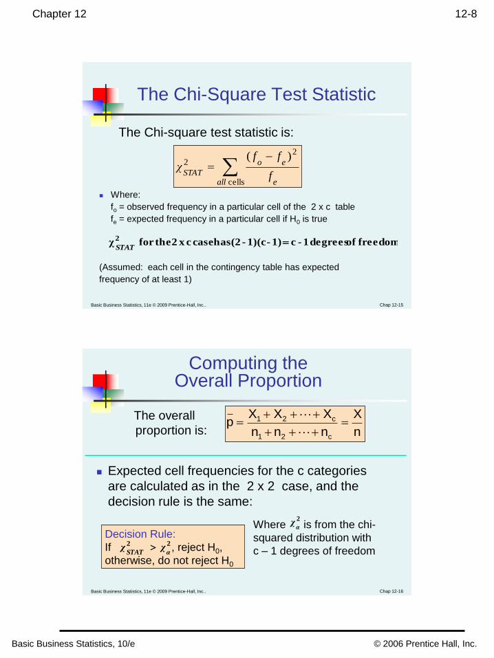
The Chi-Square Test Statistic
Where:
fo = observed frequency in a particular cell of the 2 x c table
fe = expected frequency in a particular cell if H0 is true
(Assumed: each cell in the contingency table has expected
frequency of at least 1)
cells
2
2)(
all e
eo
STAT f
ffχ
The Chi-square test statistic is:
freedom of degrees 1-c 1)-1)(c-(2 has case cx 2 thefor χ2 STAT
Basic Business Statistics, 11e © 2009 Prentice-Hall, Inc.. Chap 12-16
Computing the Overall Proportion
n
X
nnn
XXXp
c21
c21
The overall
proportion is:
Expected cell frequencies for the c categories
are calculated as in the 2 x 2 case, and the
decision rule is the same:
Where is from the chi-
squared distribution with
c – 1 degrees of freedom
Decision Rule:
If , reject H0,
otherwise, do not reject H0
22
αSTAT χ χ
2
αχ

Chapter 12 12-9
Basic Business Statistics, 10/e © 2006 Prentice Hall, Inc.
Basic Business Statistics, 11e © 2009 Prentice-Hall, Inc.. Chap 12-17
The Marascuilo Procedure
Used when the null hypothesis of equal
proportions is rejected
Enables you to make comparisons between all
pairs
Start with the observed differences, pj – pj’, for all pairs (for j ≠ j’) . . .
. . .then compare the absolute difference to a
calculated critical range
Basic Business Statistics, 11e © 2009 Prentice-Hall, Inc.. Chap 12-18
The Marascuilo Procedure
Critical Range for the Marascuilo Procedure:
(Note: the critical range is different for each pairwise comparison)
A particular pair of proportions is significantly
different if
|pj – pj’| > critical range for j and j’
(continued)
'j
'j'j
j
jj2
n
)p(1p
n
)p(1pχrange Critical
α

Chapter 12 12-10
Basic Business Statistics, 10/e © 2006 Prentice Hall, Inc.
Basic Business Statistics, 11e © 2009 Prentice-Hall, Inc.. Chap 12-19
Marascuilo Procedure Example
A University is thinking of switching to a trimester academic
calendar. A random sample of 100 administrators, 50 students,
and 50 faculty members were surveyed
Opinion Administrators Students Faculty
Favor 63 20 37
Oppose 37 30 13
Totals 100 50 50
Using a 1% level of significance, which groups have a
different attitude?
Basic Business Statistics, 11e © 2009 Prentice-Hall, Inc.. Chap 12-20
Chi-Square Test Results
Chi-Square Test: Administrators, Students, Faculty
Admin Students Faculty Total
Favor 63 20 37 120
60 30 30
Oppose 37 30 13 80
40 20 20
Total 100 50 50 200
ObservedExpected
H0: π1 = π2 = π3
H1: Not all of the πj are equal (j = 1, 2, 3)
0
2
010
2 Hreject so 9.2103 79212 .STAT
χ.χ

Chapter 12 12-11
Basic Business Statistics, 10/e © 2006 Prentice Hall, Inc.
Basic Business Statistics, 11e © 2009 Prentice-Hall, Inc.. Chap 12-21
Marascuilo Procedure: Solution
Marascuilo Procedure
Sample Sample Absolute Std. Error Critical
Group Proportion Size ComparisonDifference of Difference Range Results
1 0.63 100 1 to 2 0.23 0.084445249 0.2563 Means are not different
2 0.4 50 1 to 3 0.11 0.078606615 0.2386 Means are not different
3 0.74 50 2 to 3 0.34 0.092994624 0.2822 Means are different
0.01 9.2103
2
3.034854
Chi-sq Critical Value
Other Data
d.f
Q Statistic
Level of significance
Excel Output:
compare
At 1% level of significance, there is evidence of a difference
in attitude between students and faculty
Basic Business Statistics, 11e © 2009 Prentice-Hall, Inc.. Chap 12-22
2 Test of Independence
Similar to the 2 test for equality of more than
two proportions, but extends the concept to
contingency tables with r rows and c columns
H0: The two categorical variables are independent
(i.e., there is no relationship between them)
H1: The two categorical variables are dependent
(i.e., there is a relationship between them)
Chapter 12 12-12
Basic Business Statistics, 10/e © 2006 Prentice Hall, Inc.
Basic Business Statistics, 11e © 2009 Prentice-Hall, Inc.. Chap 12-23
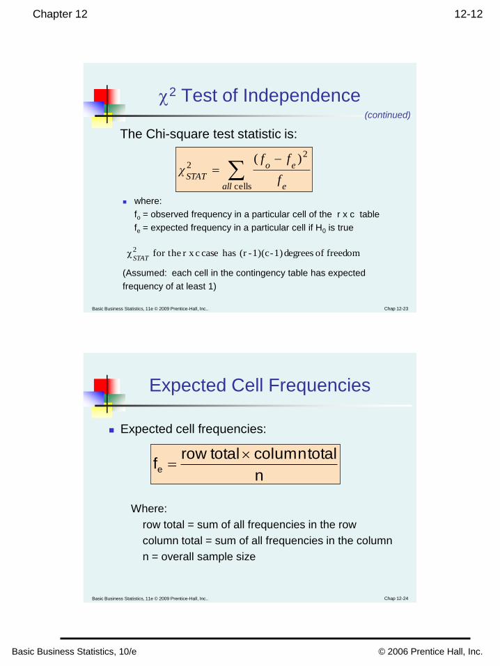
2 Test of Independence
where:
fo = observed frequency in a particular cell of the r x c table
fe = expected frequency in a particular cell if H0 is true
(Assumed: each cell in the contingency table has expected
frequency of at least 1)
cells
2
2)(
all e
eo
STAT f
ffχ
The Chi-square test statistic is:
(continued)
freedom of degrees 1)-1)(c-(r has case cr x for the χ 2
STAT
Basic Business Statistics, 11e © 2009 Prentice-Hall, Inc.. Chap 12-24
Expected Cell Frequencies
Expected cell frequencies:
n
total columntotalrow fe
Where:
row total = sum of all frequencies in the row
column total = sum of all frequencies in the column
n = overall sample size

Chapter 12 12-13
Basic Business Statistics, 10/e © 2006 Prentice Hall, Inc.
Basic Business Statistics, 11e © 2009 Prentice-Hall, Inc.. Chap 12-25
Decision Rule
The decision rule is
Where is from the chi-squared distribution
with (r – 1)(c – 1) degrees of freedom
If , reject H0,
otherwise, do not reject H0
22
αSTAT χ χ
2
αχ
Basic Business Statistics, 11e © 2009 Prentice-Hall, Inc.. Chap 12-26
Example
The meal plan selected by 200 students is shown below:
Class
Standing
Number of meals per week
Total20/week 10/week none
Fresh. 24 32 14 70
Soph. 22 26 12 60
Junior 10 14 6 30
Senior 14 16 10 40
Total 70 88 42 200
Chapter 12 12-14
Basic Business Statistics, 10/e © 2006 Prentice Hall, Inc.
Basic Business Statistics, 11e © 2009 Prentice-Hall, Inc.. Chap 12-27
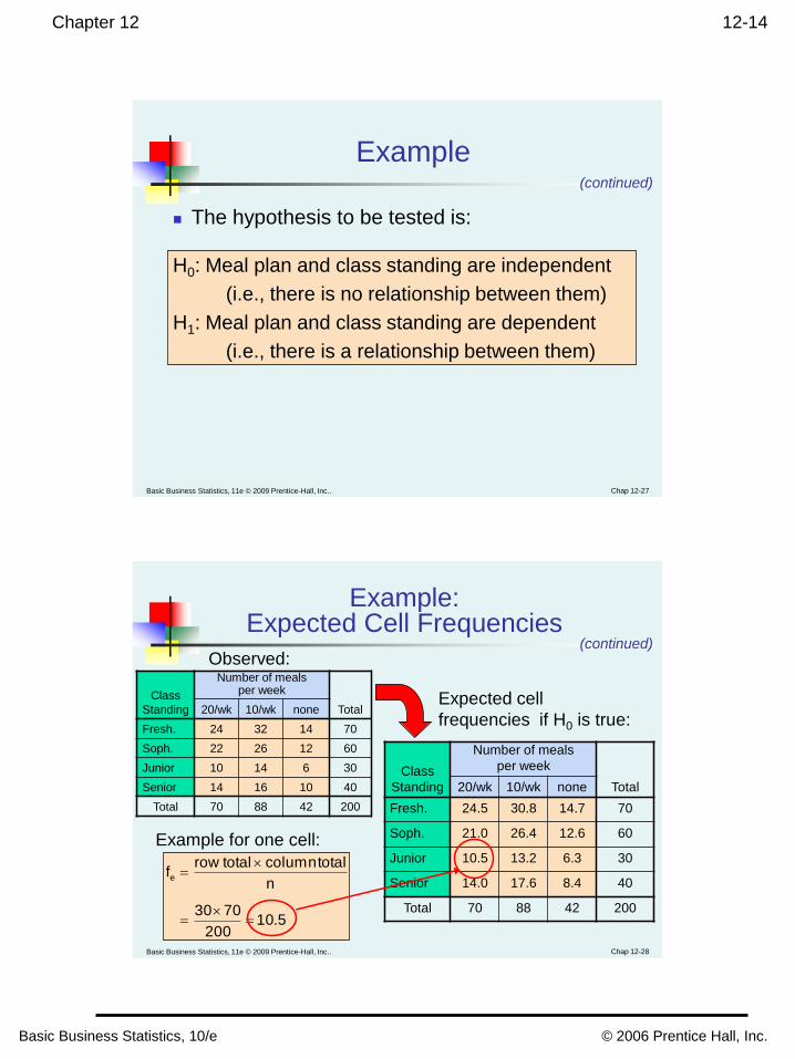
Example
The hypothesis to be tested is:
(continued)
H0: Meal plan and class standing are independent
(i.e., there is no relationship between them)
H1: Meal plan and class standing are dependent
(i.e., there is a relationship between them)
Basic Business Statistics, 11e © 2009 Prentice-Hall, Inc.. Chap 12-28
Class
Standing
Number of meals per week
Total20/wk 10/wk none
Fresh. 24 32 14 70
Soph. 22 26 12 60
Junior 10 14 6 30
Senior 14 16 10 40
Total 70 88 42 200
Class
Standing
Number of meals
per week
Total20/wk 10/wk none
Fresh. 24.5 30.8 14.7 70
Soph. 21.0 26.4 12.6 60
Junior 10.5 13.2 6.3 30
Senior 14.0 17.6 8.4 40
Total 70 88 42 200
Observed:
Expected cell
frequencies if H0 is true:
5.10200
7030
n
total columntotalrow fe
Example for one cell:
Example: Expected Cell Frequencies
(continued)

Chapter 12 12-15
Basic Business Statistics, 10/e © 2006 Prentice Hall, Inc.
Basic Business Statistics, 11e © 2009 Prentice-Hall, Inc.. Chap 12-29
Example: The Test Statistic
The test statistic value is:
709048
4810
830
83032
524
52424 222
cells
2
2
..
).(
.
).(
.
).(
f
)ff(χ
all e
eo
STAT
(continued)
= 12.592 from the chi-squared distribution
with (4 – 1)(3 – 1) = 6 degrees of freedom
2
050.χ
Basic Business Statistics, 11e © 2009 Prentice-Hall, Inc.. Chap 12-30
Example: Decision and Interpretation
(continued)
Decision Rule:
If > 12.592, reject H0,
otherwise, do not reject H0
12.592 d.f. 6 with ; 7090 is statistictest The2
050
2 .STAT
χ.χ
Here,
= 0.709 < = 12.592,
so do not reject H0
Conclusion: there is not
sufficient evidence that meal
plan and class standing are
related at = 0.05
2
20.05=12.592
0
0.05
Reject H0Do not reject H0
2
STATχ
2
STATχ 2
050.χ
Chapter 12 12-16
Basic Business Statistics, 10/e © 2006 Prentice Hall, Inc.
Basic Business Statistics, 11e © 2009 Prentice-Hall, Inc.. Chap 12-31
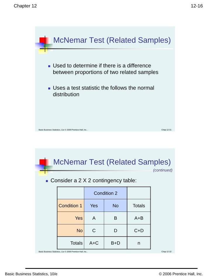
McNemar Test (Related Samples)
Used to determine if there is a difference
between proportions of two related samples
Uses a test statistic the follows the normal
distribution
Basic Business Statistics, 11e © 2009 Prentice-Hall, Inc.. Chap 12-32
McNemar Test (Related Samples)
Consider a 2 X 2 contingency table:
(continued)
Condition 2
Condition 1 Yes No Totals
Yes A B A+B
No C D C+D
Totals A+C B+D n

Chapter 12 12-17
Basic Business Statistics, 10/e © 2006 Prentice Hall, Inc.
Basic Business Statistics, 11e © 2009 Prentice-Hall, Inc.. Chap 12-33
McNemar Test (Related Samples)
The sample proportions of interest are
Test H0: π1 = π2
(the two population proportions are equal)
H1: π1 ≠ π2
(the two population proportions are not equal)
(continued)
2 condition to yesanswer whosrespondent of proportionn
CAp
1 condition to yesanswer whosrespondent of proportionn
BAp
2
1
Basic Business Statistics, 11e © 2009 Prentice-Hall, Inc.. Chap 12-34
McNemar Test (Related Samples)
The test statistic for the McNemar test:
where the test statistic Z is approximately
normally distributed
(continued)
CB
CBZ
STAT

Chapter 12 12-18
Basic Business Statistics, 10/e © 2006 Prentice Hall, Inc.
Basic Business Statistics, 11e © 2009 Prentice-Hall, Inc.. Chap 12-35
McNemar Test
Example
Suppose you survey 300 homeowners and
ask them if they are interested in refinancing
their home. In an effort to generate business,
a mortgage company improved their loan
terms and reduced closing costs. The same
homeowners were again surveyed.
Determine if change in loan terms was
effective in generating business for the
mortgage company. The data are
summarized as follows:
Basic Business Statistics, 11e © 2009 Prentice-Hall, Inc.. Chap 12-36
McNemar Test
Example
Survey response
before change
Survey response after change
Yes No Totals
Yes 118 2 120
No 22 158 180
Totals 140 160 300
Test the hypothesis (at the 0.05 level of significance):
H0: π1 ≥ π2: The change in loan terms was ineffective
H1: π1 < π2: The change in loan terms increased business
Chapter 12 12-19
Basic Business Statistics, 10/e © 2006 Prentice Hall, Inc.
Basic Business Statistics, 11e © 2009 Prentice-Hall, Inc.. Chap 12-37
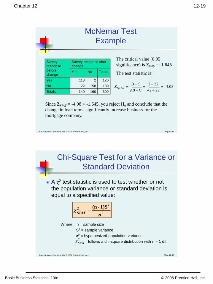
McNemar Test
Example
Survey
response
before
change
Survey response after
change
Yes No Totals
Yes 118 2 120
No 22 158 180
Totals 140 160 300
The critical value (0.05
significance) is Z0.05 = -1.645
The test statistic is:
08.4222
222
CB
CBZSTAT
Since ZSTAT = -4.08 < -1.645, you reject H0 and conclude that the
change in loan terms significantly increase business for the
mortgage company.
Basic Business Statistics, 11e © 2009 Prentice-Hall, Inc.. Chap 12-38
Chi-Square Test for a Variance or
Standard Deviation
A χ2 test statistic is used to test whether or not
the population variance or standard deviation is
equal to a specified value:
Where n = sample size
S2 = sample variance
σ2 = hypothesized population variance
follows a chi-square distribution with n – 1 d.f.
2
22
σ
1)S-(n
STATχ
2
STATχ

Chapter 12 12-20
Basic Business Statistics, 10/e © 2006 Prentice Hall, Inc.
Basic Business Statistics, 11e © 2009 Prentice-Hall, Inc.. Chap 12-39
Wilcoxon Rank-Sum Test for Differences in 2 Medians
Test two independent population medians
Populations need not be normally distributed
Distribution free procedure
Used when only rank data are available
Must use normal approximation if either of the
sample sizes is larger than 10
Basic Business Statistics, 11e © 2009 Prentice-Hall, Inc.. Chap 12-40
Wilcoxon Rank-Sum Test: Small Samples
Can use when both n1 , n2 ≤ 10
Assign ranks to the combined n1 + n2 sample
observations
If unequal sample sizes, let n1 refer to smaller-sized
sample
Smallest value rank = 1, largest value rank = n1 + n2
Assign average rank for ties
Sum the ranks for each sample: T1 and T2
Obtain test statistic, T1 (from smaller sample)

Chapter 12 12-21
Basic Business Statistics, 10/e © 2006 Prentice Hall, Inc.
Basic Business Statistics, 11e © 2009 Prentice-Hall, Inc.. Chap 12-41
Checking the Rankings
The sum of the rankings must satisfy the
formula below
Can use this to verify the sums T1 and T2
2
1)n(nTT 21
where n = n1 + n2
Basic Business Statistics, 11e © 2009 Prentice-Hall, Inc.. Chap 12-42
Wilcoxon Rank-Sum Test:Hypothesis and Decision Rule
H0: M1 = M2
H1: M1 M2
H0: M1 M2
H1: M1 M2
H0: M1 M2
H1: M1 < M2
Two-Tail Test Left-Tail Test Right-Tail Test
M1 = median of population 1; M2 = median of population 2
Reject
T1L T1U
RejectDo Not
RejectReject
T1L
Do Not Reject
T1U
RejectDo Not Reject
Test statistic = T1 (Sum of ranks from smaller sample)
Reject H0 if T1 ≤ T1L
or if T1 ≥ T1U
Reject H0 if T1 ≤ T1L Reject H0 if T1 ≥ T1U

Chapter 12 12-22
Basic Business Statistics, 10/e © 2006 Prentice Hall, Inc.
Basic Business Statistics, 11e © 2009 Prentice-Hall, Inc.. Chap 12-43
Sample data are collected on the capacity rates
(% of capacity) for two factories.
Are the median operating rates for two factories
the same?
For factory A, the rates are 71, 82, 77, 94, 88
For factory B, the rates are 85, 82, 92, 97
Test for equality of the population medians
at the 0.05 significance level
Wilcoxon Rank-Sum Test: Small Sample Example
Basic Business Statistics, 11e © 2009 Prentice-Hall, Inc.. Chap 12-44
Wilcoxon Rank-Sum Test: Small Sample Example
Capacity Rank
Factory A Factory B Factory A Factory B
71 1
77 2
82 3.5
82 3.5
85 5
88 6
92 7
94 8
97 9
Rank Sums: 20.5 24.5
Tie in 3rd and
4th places
Ranked
Capacity
values:
(continued)

Chapter 12 12-23
Basic Business Statistics, 10/e © 2006 Prentice Hall, Inc.
Basic Business Statistics, 11e © 2009 Prentice-Hall, Inc.. Chap 12-45
Wilcoxon Rank-Sum Test: Small Sample Example
(continued)
Factory B has the smaller sample size, so
the test statistic is the sum of the
Factory B ranks:
T1 = 24.5
The sample sizes are:
n1 = 4 (factory B)
n2 = 5 (factory A)
The level of significance is = .05
Basic Business Statistics, 11e © 2009 Prentice-Hall, Inc.. Chap 12-46
n2
n1
One-
Tailed
Two-
Tailed4 5
4
5
.05 .10 12, 28 19, 36
.025 .05 11, 29 17, 38
.01 .02 10, 30 16, 39
.005 .01 --, -- 15, 40
6
Wilcoxon Rank-Sum Test: Small Sample Example
Lower and
Upper
Critical
Values for
T1 from
Appendix
table E.8:
(continued)
T1L = 11 and T1U = 29

Chapter 12 12-24
Basic Business Statistics, 10/e © 2006 Prentice Hall, Inc.
Basic Business Statistics, 11e © 2009 Prentice-Hall, Inc.. Chap 12-47
H0: M1 = M2
H1: M1 M2
Two-Tail Test
Reject
T1L=11 T1U=29
RejectDo Not
Reject
Reject H0 if T1 ≤ T1L=11
or if T1 ≥ T1U=29
= .05
n1 = 4 , n2 = 5 Test Statistic (Sum of
ranks from smaller sample):
T1 = 24.5
Decision:
Conclusion:
Do not reject at = 0.05
There is not enough evidence to
prove that the medians are not
equal.
Wilcoxon Rank-Sum Test:Small Sample Solution
(continued)
Basic Business Statistics, 11e © 2009 Prentice-Hall, Inc.. Chap 12-48
Wilcoxon Rank-Sum Test (Large Sample)
For large samples, the test statistic T1 is
approximately normal with mean and
standard deviation :
Must use the normal approximation if either n1
or n2 > 10
Assign n1 to be the smaller of the two sample sizes
Can use the normal approximation for small samples
1Tμ
1Tσ
2
)1(1
1
nnTμ
12
)1n(nnσ 21
T1

Chapter 12 12-25
Basic Business Statistics, 10/e © 2006 Prentice Hall, Inc.
Basic Business Statistics, 11e © 2009 Prentice-Hall, Inc.. Chap 12-49
Wilcoxon Rank-Sum Test (Large Sample)
The Z test statistic is
Where ZSTAT approximately follows a
standardized normal distribution
12
1)(nnn
2
1)(nnT
σ
μT
Z
21
1
1
T
T1
1
1
STAT
(continued)
Basic Business Statistics, 11e © 2009 Prentice-Hall, Inc.. Chap 12-50
Wilcoxon Rank-Sum Test: Normal Approximation Example
Use the setting of the prior example:
The sample sizes were:
n1 = 4 (factory B)
n2 = 5 (factory A)
The level of significance was α = .05
The test statistic was T1 = 24.5

Chapter 12 12-26
Basic Business Statistics, 10/e © 2006 Prentice Hall, Inc.
Basic Business Statistics, 11e © 2009 Prentice-Hall, Inc.. Chap 12-51
Wilcoxon Rank-Sum Test: Normal Approximation Example
The test statistic is
202
)19(4
2
)1n(nμ 1
T1
082412
1954
12
1σ 21
1
.)()()n(nn
T
(continued)
1014.0882
20524
σ
μ
Z
1
11
..
T
T
T
STAT
Z = 1.10 is not greater than the critical Z value of 1.96
(for α = .05) so we do not reject H0 – there is not
sufficient evidence that the medians are not equal
Basic Business Statistics, 11e © 2009 Prentice-Hall, Inc.. Chap 12-52
Wilcoxon Signed Ranks Test
A nonparametric test for two related populations
Steps:
1. For each of n sample items, compute the difference,
Di, between two measurements
2. Ignore + and – signs and find the absolute values, |Di|
3. Omit zero differences, so sample size is n’
4. Assign ranks Ri from 1 to n’ (give average rank to
ties)
5. Reassign + and – signs to the ranks Ri
6. Compute the Wilcoxon test statistic W as the sum of
the positive ranks

Chapter 12 12-27
Basic Business Statistics, 10/e © 2006 Prentice Hall, Inc.
Basic Business Statistics, 11e © 2009 Prentice-Hall, Inc.. Chap 12-53
Wilcoxon Signed Ranks
Test Statistic
The Wilcoxon signed ranks test statistic is the
sum of the positive ranks:
For small samples (n’ < 20), use Table E.9 for
the critical value of W
n'
1i
)(
iRW
Basic Business Statistics, 11e © 2009 Prentice-Hall, Inc.. Chap 12-54
Wilcoxon Signed Ranks
Test Statistic
For samples of n’ > 20, W is approximately
normally distributed with
24
1)1)(2n'(n'n'σ
4
1)(n'n'μ
W
W

Chapter 12 12-28
Basic Business Statistics, 10/e © 2006 Prentice Hall, Inc.
Basic Business Statistics, 11e © 2009 Prentice-Hall, Inc.. Chap 12-55
Wilcoxon Signed Ranks Test
The large sample Wilcoxon signed ranks Z test statistic is
To test for no median difference in the paired values:
H0: MD = 0
H1: MD ≠ 0
24
1)1)(2n'(n'n'
4
1)(n'n'W
ZSTAT
Basic Business Statistics, 11e © 2009 Prentice-Hall, Inc.. Chap 12-56
Kruskal-Wallis Rank Test
Tests the equality of more than 2 population medians
Use when the normality assumption for one-way ANOVA is violated
Assumptions: The samples are random and independent
Variables have a continuous distribution
The data can be ranked
Populations have the same variability
Populations have the same shape

Chapter 12 12-29
Basic Business Statistics, 10/e © 2006 Prentice Hall, Inc.
Basic Business Statistics, 11e © 2009 Prentice-Hall, Inc.. Chap 12-57
Kruskal-Wallis Test Procedure
Obtain rankings for each value
In event of tie, each of the tied values gets the
average rank
Sum the rankings for data from each of the c
groups
Compute the H test statistic
Basic Business Statistics, 11e © 2009 Prentice-Hall, Inc.. Chap 12-58
Kruskal-Wallis Test Procedure
The Kruskal-Wallis H-test statistic: (with c – 1 degrees of freedom)
)1n(3n
T
)1n(n
12H
c
1j j
2
j
where:
n = sum of sample sizes in all groups
c = Number of groups
Tj = Sum of ranks in the jth group
nj = Number of values in the jth group (j = 1, 2, … , c)
(continued)
Chapter 12 12-30
Basic Business Statistics, 10/e © 2006 Prentice Hall, Inc.
Basic Business Statistics, 11e © 2009 Prentice-Hall, Inc.. Chap 12-59
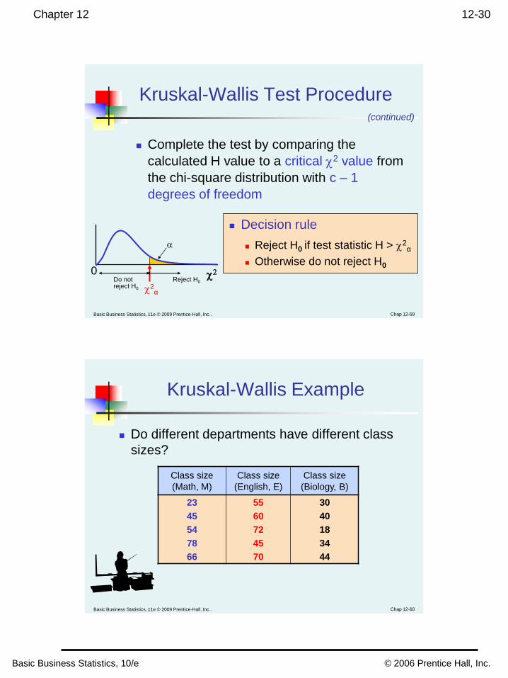
Decision rule
Reject H0 if test statistic H > 2α
Otherwise do not reject H0
(continued)
Kruskal-Wallis Test Procedure
Complete the test by comparing the
calculated H value to a critical 2 value from
the chi-square distribution with c – 1
degrees of freedom
2
2α
0
Reject H0Do not reject H0
Basic Business Statistics, 11e © 2009 Prentice-Hall, Inc.. Chap 12-60
Do different departments have different class
sizes?
Kruskal-Wallis Example
Class size
(Math, M)
Class size
(English, E)
Class size
(Biology, B)
23
45
54
78
66
55
60
72
45
70
30
40
18
34
44

Chapter 12 12-31
Basic Business Statistics, 10/e © 2006 Prentice Hall, Inc.
Basic Business Statistics, 11e © 2009 Prentice-Hall, Inc.. Chap 12-61
Do different departments have different class
sizes?
Kruskal-Wallis Example
Class size
(Math, M)Ranking
Class size
(English, E)Ranking
Class size
(Biology, B)Ranking
23
41
54
78
66
2
6
9
15
12
55
60
72
45
70
10
11
14
8
13
30
40
18
34
44
3
5
1
4
7
= 44 = 56 = 20
(continued)
Basic Business Statistics, 11e © 2009 Prentice-Hall, Inc.. Chap 12-62
The H statistic is
(continued)
Kruskal-Wallis Example
7.121)3(155
19
5
55.5
5
45.5
1)15(15
12
1)3(nn
T
1)n(n
12H
222
c
1j j
2
j
equal are Medians population allNot :H
MedianMedianMedian :H
1
BEM0

Chapter 12 12-32
Basic Business Statistics, 10/e © 2006 Prentice Hall, Inc.
Basic Business Statistics, 11e © 2009 Prentice-Hall, Inc.. Chap 12-63
Since H = 7.12 > ,
reject H0
(continued)
Kruskal-Wallis Example
5.991205.0 χ
Compare H = 7.12 to the critical value from the
chi-square distribution for 3 – 1 = 2 degrees of
freedom and = 0.05:
5.991χ 2
0.05
There is sufficient evidence to reject that
the population medians are all equal
Basic Business Statistics, 11e © 2009 Prentice-Hall, Inc.. Chap 12-64
Friedman Rank Test
Use the Friedman rank test to determine
whether c groups (i.e., treatment levels) have
been selected from populations having equal
medians
H0: M.1 = M.2 = . . . = M.c
H1: Not all M.j are equal (j = 1, 2, …, c)

Chapter 12 12-33
Basic Business Statistics, 10/e © 2006 Prentice Hall, Inc.
Basic Business Statistics, 11e © 2009 Prentice-Hall, Inc.. Chap 12-65
Friedman Rank Test
Friedman rank test for differences among c
medians:
where = the square of the total ranks for group j
r = the number of blocks
c = the number of groups
(continued)
1)3r(cR1)rc(c
12F
c
1j
2
.jR
2
.jR
Basic Business Statistics, 11e © 2009 Prentice-Hall, Inc.. Chap 12-66
Friedman Rank Test
The Friedman rank test statistic is approximated
by a chi-square distribution with c – 1 d.f.
Reject H0 if
Otherwise do not reject H0
(continued)
2
RχFα
Chapter 12 12-34
Basic Business Statistics, 10/e © 2006 Prentice Hall, Inc.
Basic Business Statistics, 11e © 2009 Prentice-Hall, Inc.. Chap 12-67
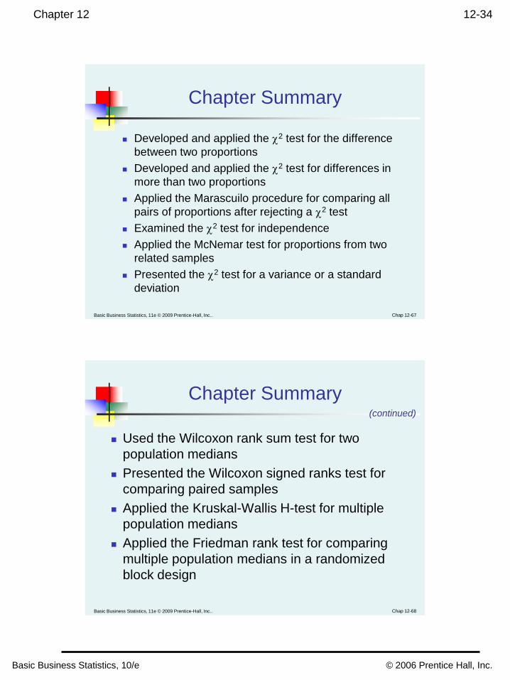
Chapter Summary
Developed and applied the 2 test for the difference
between two proportions
Developed and applied the 2 test for differences in
more than two proportions
Applied the Marascuilo procedure for comparing all
pairs of proportions after rejecting a 2 test
Examined the 2 test for independence
Applied the McNemar test for proportions from two
related samples
Presented the 2 test for a variance or a standard
deviation
Basic Business Statistics, 11e © 2009 Prentice-Hall, Inc.. Chap 12-68
Chapter Summary
Used the Wilcoxon rank sum test for two
population medians
Presented the Wilcoxon signed ranks test for
comparing paired samples
Applied the Kruskal-Wallis H-test for multiple
population medians
Applied the Friedman rank test for comparing
multiple population medians in a randomized
block design
(continued)