article info - ijgsep.com · identify the critical erosion prone areas of the watershed for...

International Journal of Geosciences and Environment Planning, Vol. 1, No. 3, Autumn 2016 71

Mapping Soil Erosion and Sediment Yield Susceptibility Using RUSLE Model (A Case Study, Ilam Dam

Watershed-Upper part, Iran)

Seyedeh Fatemeh Mousavia, Ali Janabi Naminb , Akbar Norouzi Shokrluc,1

* , Seyed Javad Sadatinejad d,

Hamed Mahmoudic

a.Master of science Student at the University of Kashan, Faculty of Agriculture and Natural Resources, Kashan,

Isfahan, Iran b. M.Sc Graduate of Watershed Management Engineering at the University of Mohagheghe Ardabili, Department of

Range and Watershed Management, Ardabil, Iran c Ph.D. Candidate of Watershed Management Engineering at the University of Shahrekord, Chaharmahale

Bakhtiari, Department of Range and Watershed Management, Shahrekord, Iran d. Associate Professor at the Tehran University, Department of Renewable Energy and the Environment

1

Corresponding author. Tel.:+989394013466 E-mail address: [email protected]

Article info Abstract

Article history: Received 26 Novemver 2016 Accepted 20 April 2017 Available online 21 May 2017

Ilam dam watershed is divided into 50×50 m grid cells and Average Annual Soil Loss and Sediment Yields (AASL&SY) are estimated for each grid cell of the watershed to identify the critical erosion prone areas of the watershed for prioritization purpose. The Rainfall erosivity (R), Soil erodibility (K), Slope length and Steepness (LS), Crop management (C) and Conservation practice factor (P) are obtained from monthly and annual rainfall data, soil map of the region, Digital Elevation Model (DEM), Normalized Difference Vegetation Index (NDVI), and land use/land cover maps, respectively. The mean values of the R, K, LS, C and P factors are 260.90 MJ mm ha−1 h−1 year−1, 0.15 T h MJ-1 mm-1, 1.97, 0.5 and 0.21, respectively. The estimated AASL&SY are 44.69 and 14.75 t ha-1 year-1, respectively.Results show that the slope length (L) and slope steepness (S) of the RUSLE model (R2 =0.77) are the most effective factors on the controlling of soil erosion in the study area. The Sediment Delivery Ratio (SDR) of estimated annual sediment yield from the observed value is 11.03%, which is indicated an accurate estimation of sediment yield from the watershed. Moreover, the results indicate that 45.76%, 13.22%, 12.85%, 10.66%, 17.49% of the study area is classed based on actual erosion risks under minimal, low, moderate, high and extreme, respectively. Overall, the RUSLE model has suitable potential to produce accurate and inexpensive erosion and sediment yield risk maps in the areas such as the study area in Iran.

Keywords: Ilam Dam watershed (Upper part), GIS, Remote Sensing, RUSLE model, Sediment yield


INTRODUCTION Soil erosion in watershed areas and the subsequent deposition in rivers, lakes and reservoirs are of great concern for two reasons. Firstly, rich fertile soil is eroded from the watershed areas. Secondly, there is a reduction in reservoir capacity as well as degradation of downstream water quality (European Environment Agency, 1995). Although sedimentation occurs naturally, it is exacerbated by poor land use and land management practices adopted in the upland areas of watersheds. Uncontrolled deforestation due to forest fires, over grazing, incorrect methods of tillage and unscientific agriculture practices are some of the poor land management practices that accelerate soil erosion, resulting in large increases in sediment inflow into streams (Rajendra,2011). Therefore, prevention of soil erosion is of paramount importance in the management and conservation of natural resources (Sadeghi et al.; 2007).Land degradation by soil erosion is a serious problem in Iran with an estimated soil loss of 2500 ×106t year-1 and about 94% of arable lands and permanent rangelands are in the process of degradation (Programme and Budget Organization, 1996; Masoudi, 2006). In terms of erosion, Iranian soils are under a serious risk due to hilly topography, soil conditions facilitating water erosion (i.e. low organic matter, poor plant coverage due to arid and semiarid climate), and inappropriate agricultural practices (i.e. excessive soil tillage and cultivation of steep lands). This widespread problem threatens the sustainability of Ilam Dam watershed, which is the main surface source of drinking water for Ilam city, Iran. Water and soil losses are the main reasons for sediment entering the reservoir and these processes potentially reduce water quality and impact on impact on ecosystem services(Dominati et al.; 2010) . Soil erosion in this area strongly influences the ecological health of the city.To estimate soil erosion and to develop optimal soil erosion management plans, many erosion models, such as Universal Soil Loss Equation (USLE) (Wischmeier and Smith, 1978), Water Erosion Prediction Project (WEPP) (Flanagan and Nearing, 1995), Soil and Water Assessment Tool (SWAT) (Arnold et al.; 1998), and European Soil Erosion Model (EUROSEM) (Morgan et al.; 1998), have been developed and used over the years. Among these models, the USLE model has remained as the most practical method for estimating soil erosion potential in fields and estimating the effects of different control management practices on soil erosion for nearly 40 years (Kinnell, 2000; Pandey et al.; 2007). The other

process-based erosion models require intensive data and thoughtfully computation steps. The new version of the USLE model, called the Revised Universal Soil Loss Equation (RUSLE), a desktop-based model, was developed by modifying the USLE to more accurately estimate the R, K, C, P factors of the soil loss equation, and soil erosion losses (Renard et al.; 1991). RUSLE is a field scale model, thus it cannot be directly used to estimate the amount of sediment reaching downstream areas because some portion of the eroded soil may be deposited while traveling to the outlet of the watershed, or the downstream point of interest. To estimate for these processes, the Sediment Delivery Ratio (SDR) for a given watershed should be used to estimate the total sediment transported to the outlet. Erskine et al.; (2002) compared RUSLE estimated soil loss with the measured sediment yield for 12 subwatersheds in Australia. The coefficient of determination was 0.88 for this comparison, although they did not consider the sediment delivery ratio in the estimated soil erosion using RUSLE. The SDR changes in the size of the watersheds, thus, the SDR needs to be considered when RUSLE is applied for a large watershed. The application of Remote sensing and GIS techniques makes soil erosion estimation and its spatial distribution to be determined with reasonable costs and better accuracy in larger areas (Millward and Mersey, 1999; Wang et al.; 2003). A combination of Remote sensing, GIS, and RUSLE is an effective tool to estimate soil loss on a cell-by-cell basis (Millward and Mersey 1999). Boggs et al.; (2001) assessed soil erosion risk based on a simplified version of RUSLE using Digital Elevation Models (DEM) data and soil mapping units. Bartsch et al.; (2002) used GIS techniques to interpolate RUSLE parameters for determining the soil erosion risk in sample plots Camp Wiliams, Utah. Wilson and Lorang, (2000) reviewed the applications of GIS in estimating soil erosion. Wang et al.; (2003) used a sample ground dataset, Thematic Mapper (TM) images, and DEM data predict soil erosion loss through geostatistical methods. They showed that such methods provided significantly better results than using traditional methods. In general, Remote sensing data were primarily used to develop the cover-management factor image through the land-cover classifications (Millward and Mersey, 1999; Reusing et al.; 2000), while GIS tools were used for derivation of the topographic factor from DEM data, data interpolation of sample plots, calculation of soil erosion loss and sediment yield (Cerri et al.; 2001; Bartsch et al.; 2002; Wang et al.; 2003; Pandey et al.; 2009).


However, the above studies did not consider the sediment delivery ratio to estimate the sediment delivered to the downstream point of interest. Regional variations in sediment yields are very important for sediment delivery processes vary in space and time. Lin et al.; (2002) investigated the sediment delivery ratio based on the ratio receiving drainage length to total drainage length using the WinGrid System and computed soil erosion using USLE model. However, this system has separate component programs rather than being fully integrated with a GIS system. Hence, it is not readily available to soil erosion decision makers and it was developed for research purposes only. Instead of this approach, GIS-based Sediment Assessment Tool for Effective Erosion Control (SATEEC) system was used to estimate soil loss and sediment yield for any location within a watershed by a combined application of RUSLE and a spatially distributed sediment delivery ratio within the GIS software environment (Lim et al.; 2003). The input data for the SATEEC GIS system are rainfall erosivity (R), soil erodibility (K), DEM, plant cover and management practice (C) and conservation support practice (P) maps, which are the basic input maps to RUSLE. Thus, one of the advantages of using the SATEEC GIS system is that no additional input data, other than those for RUSLE are required to operate the system. Moreover, all of the functions are fully integrated and automated within the GIS system and soil erosion is not only one complex space time change process comprehensively influenced by many factors, but also a typical multi-scale (space-time) variation process(Zessner et al.; 2011; Xiao Hua et al.; 2011). Thus, with several clicks of the mouse button with SATEEC menus, users can estimate the sediment yield for every cell within a watershed.Keeping this in view, the study is planned to estimate the spatial soil loss and sediment yield in Ilam Dam watershed (Upper part) to identify the critical erosion prone areas of soil and water conservation using remote sensing and GIS. 2. MATERIAL AND METHODS 2.1. Study area The study area is a mountainous watershed, which is known as Ilam Dam watershed (Upper part), and is located in the southeast of Ilam Province in the south western of Iran. The watershed area is 13475 ha (33°23' 42.15" to 33°30' 3.2" N and 46°20' 17.23" to 46°25' 1.22" E)(Figure 1). The elevations at the highest and lowest points are 1817 m and 940 m asl, respectively. Climatic condition is semi-arid with 592.78 mm rainfall, and average temperature is 21.7 °C in summer and 4.7 °C in winter. Land use in the study area, mostly includes dry farmland, forestland, rangeland, orchard, and waterbody,

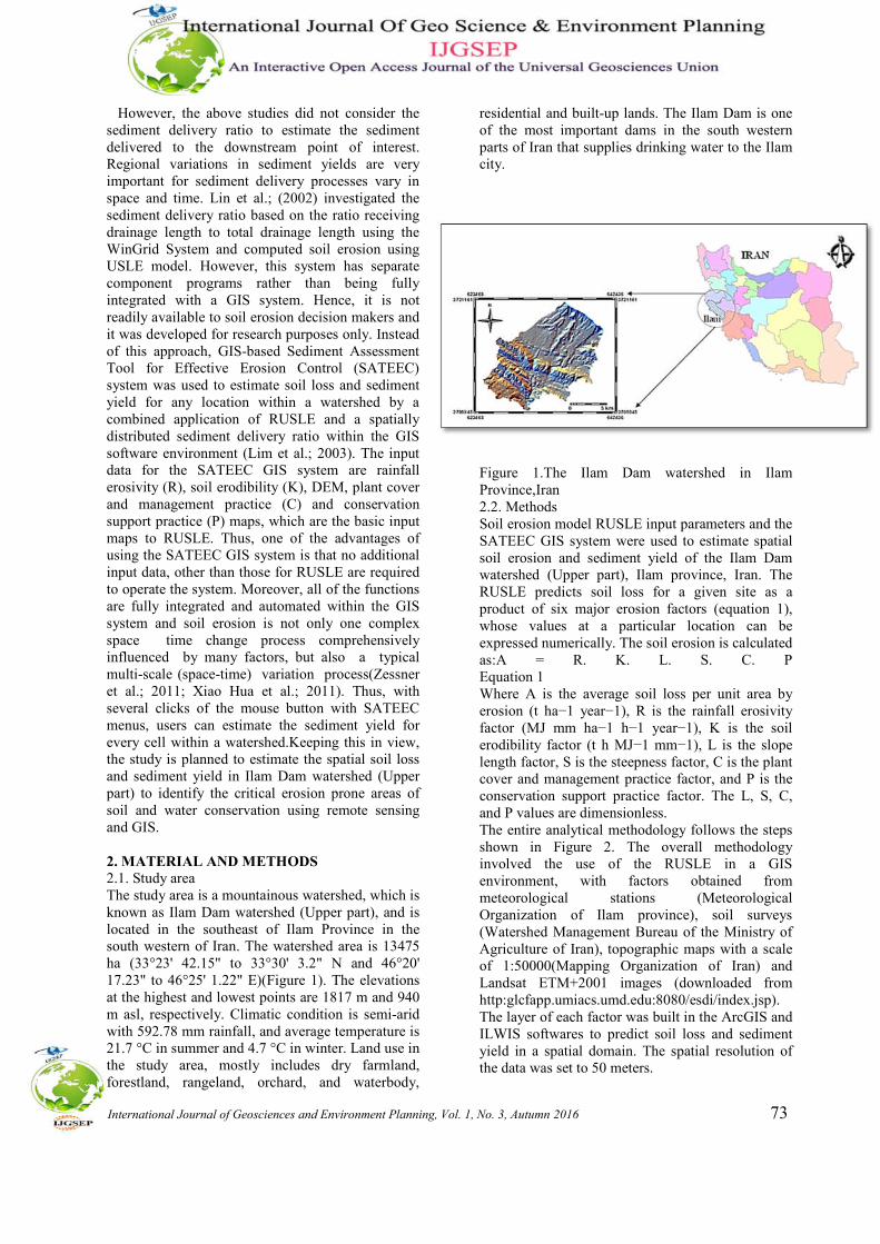
residential and built-up lands. The Ilam Dam is one of the most important dams in the south western parts of Iran that supplies drinking water to the Ilam city.

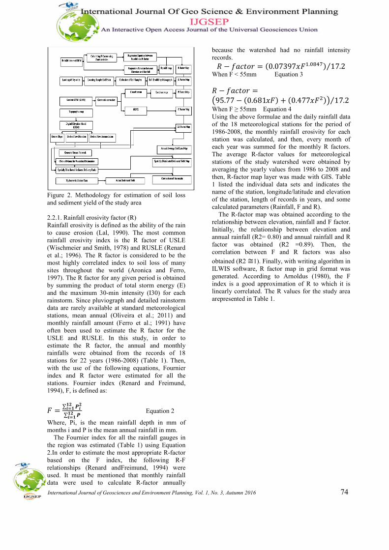
Figure 1.The Ilam Dam watershed in Ilam Province,Iran 2.2. Methods Soil erosion model RUSLE input parameters and the SATEEC GIS system were used to estimate spatial soil erosion and sediment yield of the Ilam Dam watershed (Upper part), Ilam province, Iran. The RUSLE predicts soil loss for a given site as a product of six major erosion factors (equation 1), whose values at a particular location can be expressed numerically. The soil erosion is calculated as:A = R. K. L. S. C. P Equation 1 Where A is the average soil loss per unit area by erosion (t ha−1 year−1), R is the rainfall erosivity factor (MJ mm ha−1 h−1 year−1), K is the soil erodibility factor (t h MJ−1 mm−1), L is the slope length factor, S is the steepness factor, C is the plant cover and management practice factor, and P is the conservation support practice factor. The L, S, C, and P values are dimensionless. The entire analytical methodology follows the steps shown in Figure 2. The overall methodology involved the use of the RUSLE in a GIS environment, with factors obtained from meteorological stations (Meteorological Organization of Ilam province), soil surveys (Watershed Management Bureau of the Ministry of Agriculture of Iran), topographic maps with a scale of 1:50000(Mapping Organization of Iran) and Landsat ETM+2001 images (downloaded from http:glcfapp.umiacs.umd.edu:8080/esdi/index.jsp). The layer of each factor was built in the ArcGIS and ILWIS softwares to predict soil loss and sediment yield in a spatial domain. The spatial resolution of the data was set to 50 meters.


Figure 2. Methodology for estimation of soil loss and sediment yield of the study area 2.2.1. Rainfall erosivity factor (R) Rainfall erosivity is defined as the ability of the rain to cause erosion (Lal, 1990). The most common rainfall erosivity index is the R factor of USLE (Wischmeier and Smith, 1978) and RUSLE (Renard et al.; 1996). The R factor is considered to be the most highly correlated index to soil loss of many sites throughout the world (Aronica and Ferro, 1997). The R factor for any given period is obtained by summing the product of total storm energy (E) and the maximum 30-min intensity (I30) for each rainstorm. Since pluviograph and detailed rainstorm data are rarely available at standard meteorological stations, mean annual (Oliveira et al.; 2011) and monthly rainfall amount (Ferro et al.; 1991) have often been used to estimate the R factor for the USLE and RUSLE. In this study, in order to estimate the R factor, the annual and monthly rainfalls were obtained from the records of 18 stations for 22 years (1986-2008) (Table 1). Then, with the use of the following equations, Fournier index and R factor were estimated for all the stations. Fournier index (Renard and Freimund, 1994), F, is defined as:

� =∑ ��

��

∑ ��

Equation 2

Where, Pi, is the mean rainfall depth in mm of months i and P is the mean annual rainfall in mm. The Fournier index for all the rainfall gauges in the region was estimated (Table 1) using Equation 2.In order to estimate the most appropriate R-factor based on the F index, the following R-F relationships (Renard andFreimund, 1994) were used. It must be mentioned that monthly rainfall data were used to calculate R-factor annually

because the watershed had no rainfall intensity records.

� − �� = (0.07397��.��) 17.2⁄ When F < 55mm Equation 3

� − �� =�95.77 − (0.681��)+ (0.477��)� 17.2⁄When F ≥ 55mm Equation 4 Using the above formulae and the daily rainfall data of the 18 meteorological stations for the period of 1986-2008, the monthly rainfall erosivity for each station was calculated, and then, every month of each year was summed for the monthly R factors. The average R-factor values for meteorological stations of the study watershed were obtained by averaging the yearly values from 1986 to 2008 and then, R-factor map layer was made with GIS. Table 1 listed the individual data sets and indicates the name of the station, longitude/latitude and elevation of the station, length of records in years, and some calculated parameters (Rainfall, F and R). The R-factor map was obtained according to the relationship between elevation, rainfall and F factor. Initially, the relationship between elevation and annual rainfall (R2= 0.80) and annual rainfall and R factor was obtained (R2 =0.89). Then, the correlation between F and R factors was also

obtained (R2 ≅ 1). Finally, with writing algorithm in ILWIS software, R factor map in grid format was generated. According to Arnoldus (1980), the F index is a good approximation of R to which it is linearly correlated. The R values for the study area arepresented in Table 1.


Table 1. Calculated and estimated F, R and rainfall values of the rainfall stations

Stations

Longitude

easting (UTM)

Latitude northing (UTM)

Elevation

(m)

Length of

records (years)

Rainfall values (mm)

F values

R values (MJ mm ha-1 h-1 y-

1)

Arkavaz 648478 3695819 1290 21 506.00 89.15 194 Saleh Abad 610408 3704129 620 19 341.02 67.36 108 Sarab Kalan 659379 3716270 970 11 460.89 83.89 171 Taleghani 651900 3692580 1400 8 425.22 85.09 176

Tulab 647049 3713886 1600 10 531.69 100.20 249 Gholender 651010 3723966 1045 10 488.62 91.37 205 Mishkhas 642804 3708636 1250 13 426.29 76.23 140 Karezan 641860 3733617 1280 21 583.23 101.73 257 Gonbad 643307 3680459 860 19 400.25 78.17 148 Darageh 647344 3686969 1300 10 521.25 102.14 259 Ghajar 638768 3715554 1480 8 476.10 90.67 202

Ban Rahman 626355 3669981 290 11 251.91 54.71 69 Siah Ab 639090 3689984 1220 11 440.55 91.44 205 Gol Gol 637736 3703826 1140 10 449.88 82.88 167 Gelan 617471 3698514 560 12 378.70 71.72 123 Ilam 633013 3716879 1337 22 501.50 92.29 209

Mehran 608713 3665106 200 15 200.35 38.90 4 Ema 633214 3702094 1090 19 478.69 93.61 215


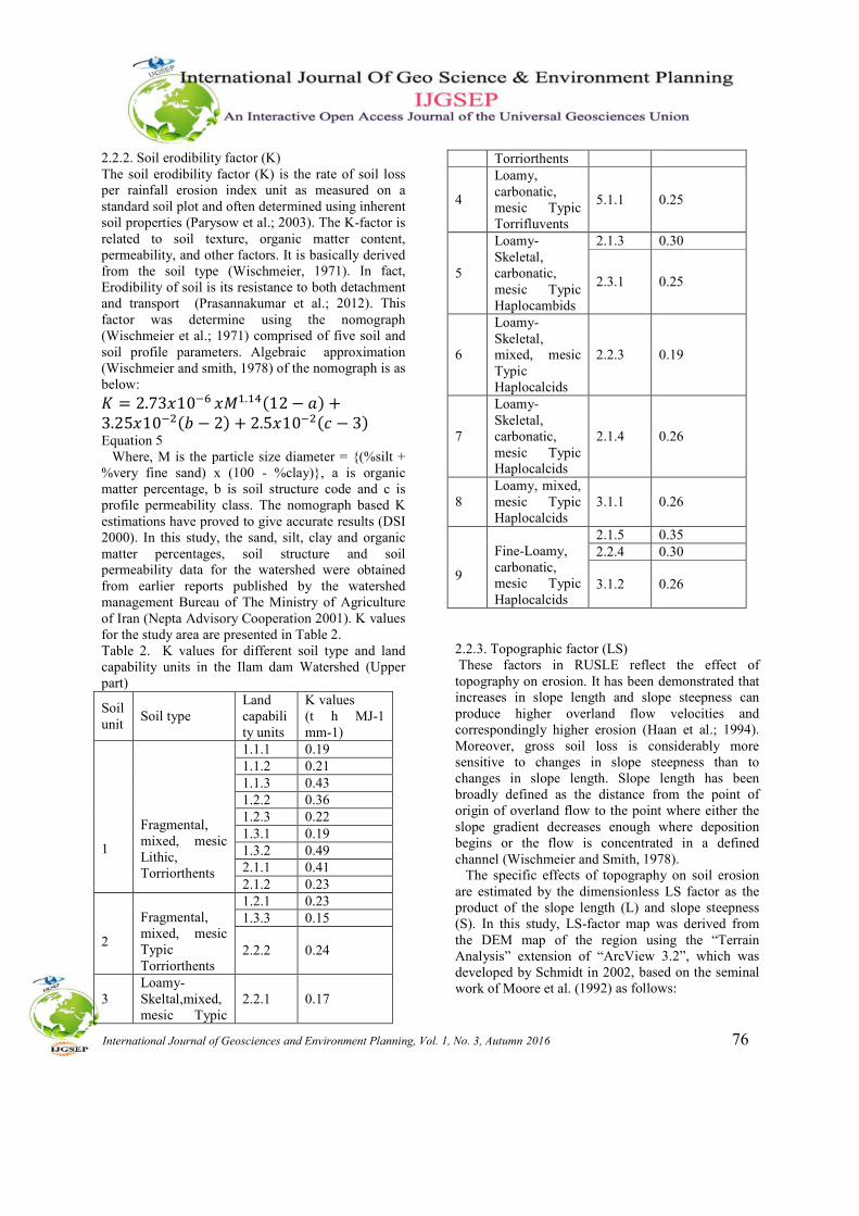
2.2.2. Soil erodibility factor (K) The soil erodibility factor (K) is the rate of soil loss per rainfall erosion index unit as measured on a standard soil plot and often determined using inherent soil properties (Parysow et al.; 2003). The K-factor is related to soil texture, organic matter content, permeability, and other factors. It is basically derived from the soil type (Wischmeier, 1971). In fact, Erodibility of soil is its resistance to both detachment and transport (Prasannakumar et al.; 2012). This factor was determine using the nomograph (Wischmeier et al.; 1971) comprised of five soil and soil profile parameters. Algebraic approximation (Wischmeier and smith, 1978) of the nomograph is as below:

� = 2.73�10�� .��(12− �)+3.25�10��(� − 2)+ 2.5�10��(� − 3) Equation 5 Where, M is the particle size diameter = {(%silt + %very fine sand) x (100 - %clay)}, a is organic matter percentage, b is soil structure code and c is profile permeability class. The nomograph based K estimations have proved to give accurate results (DSI 2000). In this study, the sand, silt, clay and organic matter percentages, soil structure and soil permeability data for the watershed were obtained from earlier reports published by the watershed management Bureau of The Ministry of Agriculture of Iran (Nepta Advisory Cooperation 2001). K values for the study area are presented in Table 2. Table 2. K values for different soil type and land capability units in the Ilam dam Watershed (Upper part)

Soil unit

Soil type Land capability units

K values (t h MJ-1 mm-1)

1

Fragmental, mixed, mesic Lithic, Torriorthents

1.1.1 0.19 1.1.2 0.21 1.1.3 0.43 1.2.2 0.36 1.2.3 0.22 1.3.1 0.19 1.3.2 0.49 2.1.1 0.41 2.1.2 0.23

2

Fragmental, mixed, mesic Typic Torriorthents

1.2.1 0.23 1.3.3 0.15

2.2.2 0.24

3 Loamy-Skeltal,mixed,mesic Typic

2.2.1 0.17

Torriorthents

4

Loamy, carbonatic, mesic Typic Torrifluvents

5.1.1 0.25

5

Loamy-Skeletal, carbonatic, mesic Typic Haplocambids

2.1.3 0.30

2.3.1 0.25

6

Loamy-Skeletal, mixed, mesic Typic Haplocalcids

2.2.3 0.19

7

Loamy-Skeletal, carbonatic, mesic Typic Haplocalcids

2.1.4 0.26

8 Loamy, mixed, mesic Typic Haplocalcids

3.1.1 0.26

9

Fine-Loamy, carbonatic, mesic Typic Haplocalcids

2.1.5 0.35 2.2.4 0.30

3.1.2 0.26

2.2.3. Topographic factor (LS) These factors in RUSLE reflect the effect of topography on erosion. It has been demonstrated that increases in slope length and slope steepness can produce higher overland flow velocities and correspondingly higher erosion (Haan et al.; 1994). Moreover, gross soil loss is considerably more sensitive to changes in slope steepness than to changes in slope length. Slope length has been broadly defined as the distance from the point of origin of overland flow to the point where either the slope gradient decreases enough where deposition begins or the flow is concentrated in a defined channel (Wischmeier and Smith, 1978). The specific effects of topography on soil erosion are estimated by the dimensionless LS factor as the product of the slope length (L) and slope steepness (S). In this study, LS-factor map was derived from the DEM map of the region using the “Terrain Analysis” extension of “ArcView 3.2”, which was developed by Schmidt in 2002, based on the seminal work of Moore et al. (1992) as follows:


L = 1.4��

��.��.� Equation 6

S = ��

�.��.�

Equation 7

Where, AS is a specific watershed area (m2/m) and β is the slope angle (degree). 2.2.4. Cover management factor (C) The C factor represents the effect of cropping and management practices in agricultural management as well as the effect of ground, tree and grass covers on reducing soil loss in non-agricultural situation (Kouli, 2009). As the vegetation cover increases, soil organic carbon accumulation increases (Lugato et al.;2014, Louwagie et al.; 2010), which in turn promotes soil aggregation and prevents erosion.. According to Biesemans et al.; (2000), C and LS are the most sensitive factors to soil loss. In the USLE/RUSLE model, the C factor is derived based on empirical equations with measurements of ground cover, aerial cover, and minimum drip height (Wischmeier and Smith, 1978). In fact the C-factor accounts for how land cover,crops and crop management cause soil loss to vary from those losses occurring in bare fallow areas (Kinnell, 2010). The most widely used indicator of vegetation growth based on the Remote Sensing technique is the Normalized Difference Vegetation Index (NDVI), which for Landsat-ETM is given by the following equation:

NDVI =��

�� Equation 8

Where NIR and R are near infrared and red band, respectively. This index is an indicator of the energy reflected by the Earth related to various cover type conditions. NDVI values range between -1.0 and +1.0. When the measured spectral response of the earth’s surface is very similar to both bands, the NDVI values approach to zero. A large difference between the two bands results in NDVI values at the extremes of the data range. Photo synthetically active vegetation presents a high reflectance in the near IR portion of the spectrum, in comparison to the visible portion. Therefore, The NDVI values for photosynthetically active vegetation will be positive. Areas with low vegetation cover or without vegetative cover (such as bare soil and urban areas) as well as inactive vegetation (unhealthy plants) will usually display NDVI values fluctuating between -0.1 and +0.1. Clouds and water bodies will give negative or zero values.

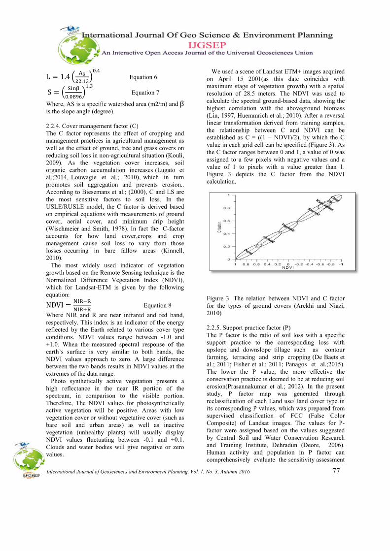
We used a scene of Landsat ETM+ images acquired on April 15 2001(as this date coincides with maximum stage of vegetation growth) with a spatial resolution of 28.5 meters. The NDVI was used to calculate the spectral ground-based data, showing the highest correlation with the aboveground biomass (Lin, 1997, Huemmrich et al.; 2010). After a reversal linear transformation derived from training samples, the relationship between C and NDVI can be established as C = ((1 − NDVI)/2), by which the C value in each grid cell can be specified (Figure 3). As the C factor ranges between 0 and 1, a value of 0 was assigned to a few pixels with negative values and a value of 1 to pixels with a value greater than 1. Figure 3 depicts the C factor from the NDVI calculation.

Figure 3. The relation between NDVI and C factor for the types of ground covers (Arekhi and Niazi, 2010) 2.2.5. Support practice factor (P) The P factor is the ratio of soil loss with a specific support practice to the corresponding loss with upslope and downslope tillage such as contour farming, terracing and strip cropping (De Baets et al.; 2011; Fisher et al.; 2011; Panagos et al.;2015). The lower the P value, the more effective the conservation practice is deemed to be at reducing soil erosion(Prasannakumar et al.; 2012). In the present study, P factor map was generated through reclassification of each Land use/ land cover type in its corresponding P values, which was prepared from supervised classification of FCC (False Color Composite) of Landsat images. The values for P-factor were assigned based on the values suggested by Central Soil and Water Conservation Research and Training Institute, Dehradun (Deore, 2006). Human activity and population in P factor can comprehensively evaluate the sensitivity assessment


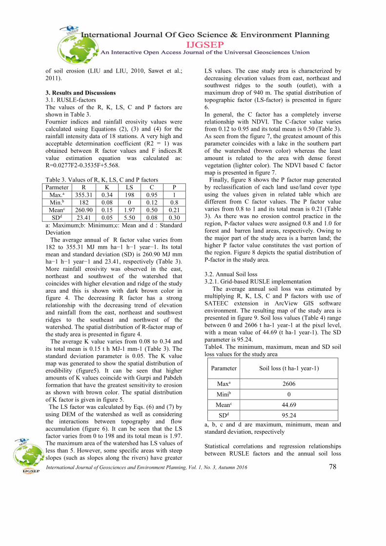
of soil erosion (LIU and LIU, 2010, Sawet et al.; 2011). 3. Results and Discussions 3.1. RUSLE-factors The values of the R, K, LS, C and P factors are shown in Table 3. Fournier indices and rainfall erosivity values were calculated using Equations (2), (3) and (4) for the rainfall intensity data of 18 stations. A very high and acceptable determination coefficient (R2 = 1) was obtained between R factor values and F indices.R value estimation equation was calculated as: R=0.0277F2-0.3535F+5.568. Table 3. Values of R, K, LS, C and P factors Parmeter R K LS C P

Max.a 355.31 0.34 198 0.95 1 Min.b 182 0.08 0 0.12 0.8 Meanc 260.90 0.15 1.97 0.50 0.21 SDd 23.41 0.05 5.50 0.08 0.30

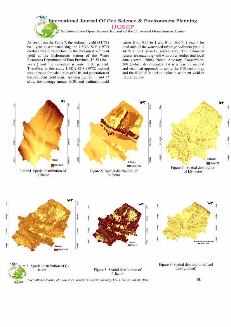
a: Maximum;b: Minimum;c: Mean and d : Standard Deviation The average annual of R factor value varies from 182 to 355.31 MJ mm ha−1 h−1 year−1. Its total mean and standard deviation (SD) is 260.90 MJ mm ha−1 h−1 year−1 and 23.41, respectively (Table 3). More rainfall erosivity was observed in the east, northeast and southwest of the watershed that coincides with higher elevation and ridge of the study area and this is shown with dark brown color in figure 4. The decreasing R factor has a strong relationship with the decreasing trend of elevation and rainfall from the east, northeast and southwest ridges to the southeast and northwest of the watershed. The spatial distribution of R-factor map of the study area is presented in figure 4. The average K value varies from 0.08 to 0.34 and its total mean is 0.15 t h MJ-1 mm-1 (Table 3). The standard deviation parameter is 0.05. The K value map was generated to show the spatial distribution of erodibility (figure5). It can be seen that higher amounts of K values coincide with Gurpi and Pabdeh formation that have the greatest sensitivity to erosion as shown with brown color. The spatial distribution of K factor is given in figure 5. The LS factor was calculated by Eqs. (6) and (7) by using DEM of the watershed as well as considering the interactions between topography and flow accumulation (figure 6). It can be seen that the LS factor varies from 0 to 198 and its total mean is 1.97. The maximum area of the watershed has LS values of less than 5. However, some specific areas with steep slopes (such as slopes along the rivers) have greater

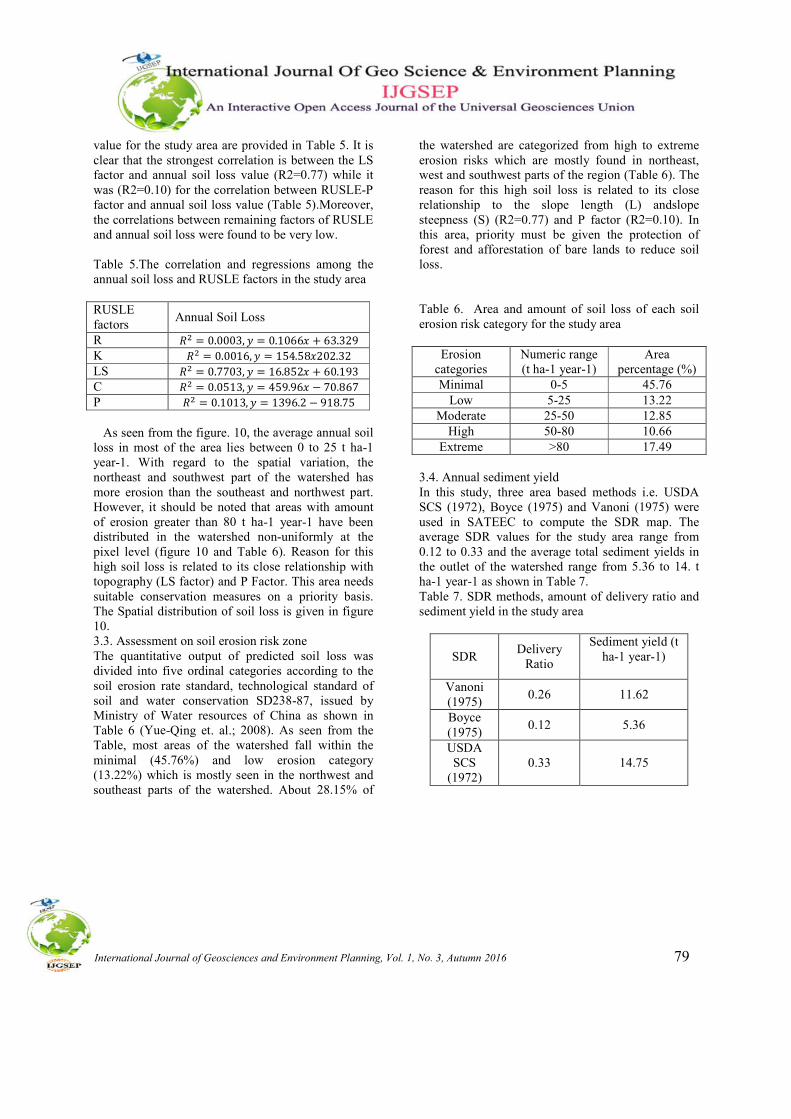
LS values. The case study area is characterized by decreasing elevation values from east, northeast and southwest ridges to the south (outlet), with a maximum drop of 940 m. The spatial distribution of topographic factor (LS-factor) is presented in figure 6. In general, the C factor has a completely inverse relationship with NDVI. The C-factor value varies from 0.12 to 0.95 and its total mean is 0.50 (Table 3). As seen from the figure 7, the greatest amount of this parameter coincides with a lake in the southern part of the watershed (brown color) whereas the least amount is related to the area with dense forest vegetation (lighter color). The NDVI based C factor map is presented in figure 7. Finally, figure 8 shows the P factor map generated by reclassification of each land use/land cover type using the values given in related table which are different from C factor values. The P factor value varies from 0.8 to 1 and its total mean is 0.21 (Table 3). As there was no erosion control practice in the region, P-factor values were assigned 0.8 and 1.0 for forest and barren land areas, respectively. Owing to the major part of the study area is a barren land; the higher P factor value constitutes the vast portion of the region. Figure 8 depicts the spatial distribution of P-factor in the study area. 3.2. Annual Soil loss 3.2.1. Grid-based RUSLE implementation The average annual soil loss was estimated by multiplying R, K, LS, C and P factors with use of SATEEC extension in ArcView GIS software environment. The resulting map of the study area is presented in figure 9. Soil loss values (Table 4) range between 0 and 2606 t ha-1 year-1 at the pixel level, with a mean value of 44.69 (t ha-1 year-1). The SD parameter is 95.24. Table4. The minimum, maximum, mean and SD soil loss values for the study area

Parameter Soil loss (t ha-1 year-1)

Maxa 2606

Minib 0

Meanc 44.69

SDd 95.24

a, b, c and d are maximum, minimum, mean and standard deviation, respectively Statistical correlations and regression relationships between RUSLE factors and the annual soil loss


value for the study area are provided in Table 5. It is clear that the strongest correlation is between the LS factor and annual soil loss value (R2=0.77) while it was (R2=0.10) for the correlation between RUSLE-P factor and annual soil loss value (Table 5).Moreover, the correlations between remaining factors of RUSLE and annual soil loss were found to be very low. Table 5.The correlation and regressions among the annual soil loss and RUSLE factors in the study area RUSLE factors

Annual Soil Loss

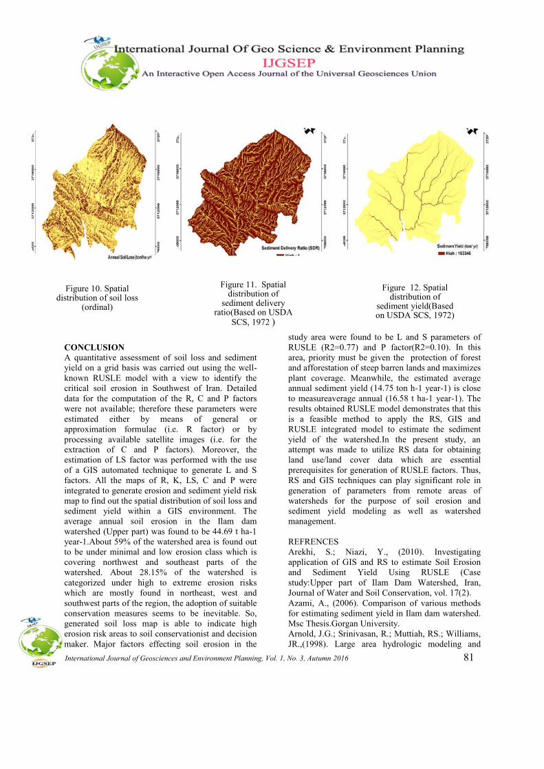
R �� = 0.0003, � = 0.1066� + 63.329 K �� = 0.0016, � = 154.58�202.32 LS �� = 0.7703, � = 16.852� + 60.193 C �� = 0.0513, � = 459.96� − 70.867 P �� = 0.1013, � = 1396.2 − 918.75 As seen from the figure. 10, the average annual soil loss in most of the area lies between 0 to 25 t ha-1 year-1. With regard to the spatial variation, the northeast and southwest part of the watershed has more erosion than the southeast and northwest part. However, it should be noted that areas with amount of erosion greater than 80 t ha-1 year-1 have been distributed in the watershed non-uniformly at the pixel level (figure 10 and Table 6). Reason for this high soil loss is related to its close relationship with topography (LS factor) and P Factor. This area needs suitable conservation measures on a priority basis. The Spatial distribution of soil loss is given in figure 10. 3.3. Assessment on soil erosion risk zone The quantitative output of predicted soil loss was divided into five ordinal categories according to the soil erosion rate standard, technological standard of soil and water conservation SD238-87, issued by Ministry of Water resources of China as shown in Table 6 (Yue-Qing et. al.; 2008). As seen from the Table, most areas of the watershed fall within the minimal (45.76%) and low erosion category (13.22%) which is mostly seen in the northwest and southeast parts of the watershed. About 28.15% of

the watershed are categorized from high to extreme erosion risks which are mostly found in northeast, west and southwest parts of the region (Table 6). The reason for this high soil loss is related to its close relationship to the slope length (L) andslope steepness (S) (R2=0.77) and P factor (R2=0.10). In this area, priority must be given the protection of forest and afforestation of bare lands to reduce soil loss. Table 6. Area and amount of soil loss of each soil erosion risk category for the study area

Erosion categories

Numeric range (t ha-1 year-1)

Area percentage (%)

Minimal 0-5 45.76 Low 5-25 13.22

Moderate 25-50 12.85 High 50-80 10.66

Extreme >80 17.49 3.4. Annual sediment yield In this study, three area based methods i.e. USDA SCS (1972), Boyce (1975) and Vanoni (1975) were used in SATEEC to compute the SDR map. The average SDR values for the study area range from 0.12 to 0.33 and the average total sediment yields in the outlet of the watershed range from 5.36 to 14. t ha-1 year-1 as shown in Table 7. Table 7. SDR methods, amount of delivery ratio and sediment yield in the study area

SDR Delivery

Ratio

Sediment yield (t ha-1 year-1)

Vanoni (1975)

0.26 11.62

Boyce (1975)

0.12 5.36

USDA SCS

(1972) 0.33 14.75


Figure4. Spatial distribution of R-factor

Figure 5. Spatial distribution of K-factor

Figure 6. Spatial distribution of LS-factor

As seen from the Table 7, the sediment yield (14.75 t ha-1 year-1) estimatedusing the USDA SCS (1972) method was almost close to the measured sediment yield at the hydrometric station of the Water Resources Department of Ilam Province (16.58 t ha-1 year-1) and the deviation is only 11.03 percent. Therefore, in this study USDA SCS (1972) method was selected for calculation of SDR and generation of the sediment yield map. As seen figures 11 and 12 show the average annual SDR and sediment yield

varies from 0.33 to 1 and 0 to 163346 t year-1 for total area of the watershed (average sediment yield is 14.75 t ha-1 year-1), respectively. The estimated results are matching well with other studies and local data (Azami 2006; Nepta Advisory Cooperation, 2001),which demonstrates that is a feasible method and technical approach to apply the GIS technology and the RUSLE Model to estimate sediment yield in Ilam Province.

Figure 7. Spatial distribution of C-factor Figure 8. Spatial distribution of

P-factor

Figure 9. Spatial distribution of soil loss (gradual)


CONCLUSION A quantitative assessment of soil loss and sediment yield on a grid basis was carried out using the well-known RUSLE model with a view to identify the critical soil erosion in Southwest of Iran. Detailed data for the computation of the R, C and P factors were not available; therefore these parameters were estimated either by means of general or approximation formulae (i.e. R factor) or by processing available satellite images (i.e. for the extraction of C and P factors). Moreover, the estimation of LS factor was performed with the use of a GIS automated technique to generate L and S factors. All the maps of R, K, LS, C and P were integrated to generate erosion and sediment yield risk map to find out the spatial distribution of soil loss and sediment yield within a GIS environment. The average annual soil erosion in the Ilam dam watershed (Upper part) was found to be 44.69 t ha-1 year-1.About 59% of the watershed area is found out to be under minimal and low erosion class which is covering northwest and southeast parts of the watershed. About 28.15% of the watershed is categorized under high to extreme erosion risks which are mostly found in northeast, west and southwest parts of the region, the adoption of suitable conservation measures seems to be inevitable. So, generated soil loss map is able to indicate high erosion risk areas to soil conservationist and decision maker. Major factors effecting soil erosion in the

study area were found to be L and S parameters of RUSLE (R2=0.77) and P factor(R2=0.10). In this area, priority must be given the protection of forest and afforestation of steep barren lands and maximizes plant coverage. Meanwhile, the estimated average annual sediment yield (14.75 ton h-1 year-1) is close to measureaverage annual (16.58 t ha-1 year-1). The results obtained RUSLE model demonstrates that this is a feasible method to apply the RS, GIS and RUSLE integrated model to estimate the sediment yield of the watershed.In the present study, an attempt was made to utilize RS data for obtaining land use/land cover data which are essential prerequisites for generation of RUSLE factors. Thus, RS and GIS techniques can play significant role in generation of parameters from remote areas of watersheds for the purpose of soil erosion and sediment yield modeling as well as watershed management. REFRENCES Arekhi, S.; Niazi, Y., (2010). Investigating application of GIS and RS to estimate Soil Erosion and Sediment Yield Using RUSLE (Case study:Upper part of Ilam Dam Watershed, Iran, Journal of Water and Soil Conservation, vol. 17(2). Azami, A., (2006). Comparison of various methods for estimating sediment yield in Ilam dam watershed. Msc Thesis.Gorgan University. Arnold, J.G.; Srinivasan, R.; Muttiah, RS.; Williams, JR.,(1998). Large area hydrologic modeling and

Figure 10. Spatial distribution of soil loss

(ordinal)

Figure 11. Spatial distribution of

sediment delivery ratio(Based on USDA

SCS, 1972 )

Figure 12. Spatial distribution of

sediment yield(Based on USDA SCS, 1972)


assessment: Part I. Model development. Journal of the American Water Resources Association 34 (1), 73– 89. Arnoldus, HMJ.,(1980). An approximation of the rainfall factor in the Universal Soil Loss Equation. In: De Boodt, M.andGabriels, D. (eds) Assessment of erosion. Wiley, Chichester, pp 127–132. Aronica, G.; Ferro, V., (1997). Rainfall erosivity over the Calabrian region. Hydrological Science Journal 42 (1), 35–48. Bartsch, KP.;Van Miegroet, H.; Boettinger, J.; Dobrwolski, JP., (2002). Using empirical erosion models and GIS to determine erosion risk at Camp Williams.Journal of soil and water conservation 57:29-37. Biesemans, J.; Meirvenne, MV.;Gabriels, D., (2000). Extending the RUSLE with the Monte Carlo error propagation technique to predict long-term average off-site sediment accumulation. J Soil Water Conserv 55:35–42. Boggs G, Devonport C, Evans K,Puig P.,(2001). GIS-based rapid assessment of erosion risk in a small catchment in the wet/dry tropics of Australia. Land Degrad. Dev. 12, 417–434. Boyce, RC., (1975). Sediment routing with sediment delivery ratios. Present and Prospective Technology for ARS. USDA, Washington, D.C. Cerri, CEP.; Dematte, JAM.; Ballester, MVR.; Martinelli, LA.; Victoria, RL.;Roose, E., (2001). GIS erosion risk assessment of the Piracicaba River Basin,southeastern Brazil,Mapping sciences and remote sensing 38:157-171. De Baets, S.; Poesen, J.; Merrsmans, J.; Serlet, L., (2011). Cover crops and their erosion-reducing effects during concentrated flow erosion. Catena 85 (3),237–244. Deore, A.; Sachin, J.,(2006). Prioritization of micro-watersheds of upper Bhama basin on the basis of soil erosion risk using remote sensing and GIS technology.Ph.D thesis. Department of Geography. University of Pune. Dominati, E.; Patterson, M.; Mackay, A., (2010).A framework for classifying and quantifying the natural capital and ecosystem services of soils. Ecol. Econ. 69 (9), 1858–1868 D.S.I, (2000). General directorate of state hydraulic works,Turkey emergency, flood and earthquake recovery project(TEFER),Sediment transport investigation in west Black sea flood region, Final report, Turkey. Erskine, WD.; Mahmoudzadeh, A.; Myers, C., (2002). Land use effects on sediment yields and soil loss rates in small basins of Triassic sandstone near Sydney, NSW, Australia. Catena 49, 271-287.

European Environment Agency,1995. CORINE soil risk and important land resources-in the southern regions of the european community, Commission of the European Communities. Fisher, K.A.; Momen, B.; Kratochvil, R.J., (2011). Is broadcasting seed an effective winter cover crop planting method, Agron. J. 103 (2), 472–478 Flanagan, D.C.; Nearing, M.A., (1995). USDA water erosion prediction project: hillslope profile and watershed model documentation. NSERL Report No. 10. USDA-ARS National soil erosion research laboratory, West Lafayette, IN 47907-1194. Haan, C.T.; Barfield, B.J.; Hayes, J.C., (1994). Design hydrology and sedimentology for small catchments. Academic Press, San Diego, 588pp. Huemmrich, K. F.; Kinoshita, G.; Gamon, J. A.; Houston, S.; Kwon, H.,(2010b). Tundra carbon balance under varying temperature and 406 moisture regimes. Journal of Geophysical Research-Biogeosciences,115. Kinnell, P.I.A., (2000). AGNPS-UM: Applying the USLE-M within the agricultural non point source pollution model. EnvironmentalModelling and Software 15 (3), 331–341. Kinnell, P.I.A. (2010). Event soil loss, runoff and the Universal Soil Loss Equation family of models: a review. J. Hydrol. 385 (1–4), 384–397. Kouli, M.; Soupios,P.; Vallianatos, F., (2009). Soil erosion prediction using the Revised Universal Soil Loss Equation(RUSLE) in a GIS framework, Chania, Northwestern Crete, Greece, Environ Geol.; 57:483-497. Lal, R., (1990). Soil erosion in the tropics. Principles and Management. McGraw-Hill, New York. 580 pp. Lim, K.J.; Choi, J.; Kim, K.; Sagong, M.; Engel, B.A., (2003). Development of sediment assessment tool for effective erosion control (SATEEC) in small scale watershed. Transactions of the Korean Society of Agricultural Engineers 45 (5), 85–96. Lin, C.; Lin, W.; Chou, W., (2002). Soil erosion prediction and sediment yield estimation: the Taiwan experience. Soil and Tillage Research 68, 143– 152. Lin, C.Y., (1997). A study on the width and placement of vegetated buffer strips in a mudstone-distributed watershed.J.china. Soil water conserve.29 (3), 250-266(in Chinese with English abstract). LIU, L.; LIU, X.H., (2010). Sensitivity analysis of soil erosion in the northern loess Plateau. Procedia environmental sciences 2 :134–148. Louwagie, G.; Gay, S.H.; Sammeth, F.; Ratinger, T., (2010). The potential of European Union policies to address soil degradation in agriculture. Land Degrad. Dev. 22(1), 5–17


Lugato, E.; Panagos, P.; Bampa, F.; Jones, A.; Montanarella, L., (2014). A new baseline of organic carbon stock in European agricultural soils using a modelling approach. Global Change Biol. 20 (1), 313–326 Masoudi, M.; Patwardhan, A.M.; Gore, S.D., (2006). Risk assessment of water erosion for the Qareh Aghaj subbasin, southern Iran. Stochastic Environmental Resources Risk Assessment. 21:15-24 Millward, A.A.; Mersey, J.E., (1999). Adapting the RUSLE to model soil erosion potential in a mountainous tropical watershed. Catena 3:109-129. Moore, I.D,Wilson, J.P., (1992). Length-slope factors for the Revised Universal Soil Loss Equation: Simplified method of estimation. Journal of Soil and Water Conservation 47:423–428. Morgan, R.P.C.; Quinton, J.N.; Smith, R.E.; Govers, G.; Poesen, J.; Auerswald, K.; Chisci, G.; Torri, D., (2001).Styczen Nepta Advisory Coopeation . Detail project of Ilam Dam watershed, Jahad and Agriculture Organization of Ilam province.; 135 p. Oliveira, P.T.S.; Rodrigues, D.B.B.; Alves, Sobrinho T.; Carvalho, D.F.; Panachuki, E.,(2011). Spatial varibility of the rainfall erosive potencial in the State of Mato Grosso do Sul, Brazil, Brazil. Engenharia Agrícola 32, 69–79.http://dx.doi.org/10.1590/S0100-69162012000100008 Panagos, P.; Borrelli, P.; Meusburger, K.; van der Zanden, E.H.; Poesen, J.; Alewell, C., (2015). Modelling the effect of support practices (P-factor) on the reduction of soil erosion by water at European Scale. Environ. Sci. Policy 51, 23–34. Pandey, A.; Chowdary, V. M.; Mal, BC., (2007). Identification of critical erosion prone areas in the small agricultural watershed using USLE, GIS and Remote Sensing. Water Resources Management (Springer).; 21(4) :729–746. Pandey, A.; Chowdary, V.M.; Mal, B.C., (2009). Sediment yield modelling of an agricultural watershed using MUSLE, Remote Sensing and GIS. Journal of Paddy Water Environment (Springer).; 7 (2): 105–113. Parysow, P.; Wang, G.X.; Gertner, G.; Anderson, A.B., (2003). Spatial uncertainty analysis for mapping soil erodibility based on joint sequential simulation. Catena 53:65–78. Prasannakumar, V.; Vijith,H.; Abinod, S.; Geetha,N.,(2012). Estimation of soil erosion risk within a small mountainous sub-watershed in Kerala, India, using Revised Universal Soil Loss Equation (RUSLE) and geo information technology. Geoscience Frontiers 3(2): 209-215.

Programme and budget organization.,(1996). First national report on human development of Iran. Rajendra, Hegde.; A. Natarajan, L .G .K.;Naidu and Dipak, S., (2011). Soil Degradation, Soil Erosion Issues in Agriculture, Dr. Danilo Godone (Ed.), ISBN: 978-953-307-435-1 Renard, K.G.; Foster, G.R.; Weesies, G.A.; McCool, D.K., (1996). Predicting soil erosion by water. A guide to conservation planning with the revised universal soil loss equation (RUSLE). Agriculture Handbook 703. US Govt Print Office, Washington, DC. Renard, K.G.;Freimund, J.R., (1994). Using monthly precipitation data to estimate the R factor in the revised USLE. Journal of Hydrology. 157:287–306. Renard, K.G.; Foster, G.R.; Weesies, G.A.; Porter, J.P., (1991). RUSLE: revised universal soil loss equation. Journal of Soil and Water Conservation 46 (1), 30– 33. Reusing, M.; Schneider, T.; Ammer, U., (2000). Modeling soil erosion rates in the Ethiopian Highlands by integration of high resolution MOMs-2/D2-stereo-data in a GIS.International Journal of Remote sensing 21:1885-1896. Sadeghi, SHR,,Ghaderi, M.;Vangah, B.; Safaeeian, N.A., (2007). Comparision between effects of open grazing and manual harvesting of cultivated summer rangelands of Northern Iran on infiltration, runoff and sediment yield. Land degradation and development (DOI/10,1002:1dr.799). Sawet, P.W. P.; and Charlie, Navanugr., (2011). Soil Erosion Analysis Using Universal Soil Loss Equation (USLE) to Estimate the Loss of Plant Nutrient in Huaimaeprachan Watershed. Journal of Social Science, Srinakharinwirot University, 14 (6). Schmidt, F.; Persson ,A ., (2002). Comparison of DEM data capture and topographic wetness indices. Precision Agriculture 4(2): 179-192 USDA., (1975). Sediment sources, yields, and delivery ratios. National Engineering Handbook, Section 3 Sedimentation. Vanoni, V.A.,(1975).Sedimentation engineering, Manual and report No. 54. American Society of Civil Engineers, New York, N.Y Wang, G.; Gertner, G.; Fang, S.; Anderson, A.B., (2003). Mapping multiple variables for predicting soil loss by geostatistical methods with TM images and a slope map.Photogrammetric Engineering and remote sensing 69:889-898. Wilson, J.P.; Lorang, M.S., (2000). Spatial models of soil erosion and GIS.In spatial models and GIS.New potential and new models,Fotheringham, A.S. and Wegener, M.(eds).Taylor and Francis:Philadelphia,PA;83-108.


Wischmeier, W.H., (1971). A soil erodibility nomograph for farmland and construction sites. Journal of Soil and Water Conservation 26:189 193. Wischmeier,WH.; Johnson, C.B.; Cross, B.V., (1971). A soil erodibility nomograph for farmland and construction sites. Journal of Soil Water Conservation 26 (5):189–193. Wischmeier, W.H.; Smith, D.D., (1978). Predicting rainfall erosion. losses: a guide to conservation planning. Agriculture Handbook, vol. 537. US Department of Agriculture, Washington,DC, 58 pp. XiaoHua, Xu.; Xin-Fa, Xu.; Sheng, Lei .; ShaSha, Fu. ; Gaowei, Wu., (2011). Soil erosion environmental analysis of the three Gorges Reservoir Area Based on the "3S" technology. Procedia Environmental Sciences 10:2218-2225.

Yue-Qing, X.;Shao, X.M.; Kong, X.B.; 2008.Adapting the RUSLE and GIS to model soil erosion risk in a mountains karst watershed,Guizhou Province,China.Environmental Monitoring Assessment.; 141:275-286. Zessner, M.; Kovacs, A.; Schilling, C.; Hochedlinger, G.; Gabriel, O.; Natho, S.; Thaler, S.; Windhofer, G.; 2011. Enhancement of the MONERIS model for application in alpine catchments in Austria, International Review of Hydrobiology.

article info - ijgsep.com · identify the critical erosion prone areas of the watershed for...

Documents