Long-range acoustic transmissions Long-range acoustic transmissions

for navigation, communication, and for navigation, communication, and

ocean observation in the Arcticocean observation in the Arctic

Alexander Gavrilov, CMST

Peter Mikhalevsky, SAIC

OUTLINE

1. Some examples of long-range acoustic transmissions in the Arctic Ocean (TAP and ACOUS experiments)

2. Numerical prediction of transmission loss at different frequencies and experimental results

3. Possible outline of the network• Navigation• Communication• Ocean Observation

4. Problems ?

TAP (blue) and ACOUS (red) experiment paths in the Arctic Ocean

APLIS

ACOUSSource

Nanse

n Bas

in

Fram

Bas

in

Greenland

RussiaCanada

Spitsbergen

1805 1810 1815 1820 1825 1830 1835

500

1000

1500

2000

2500

3000

3500

Travel time, s

Am

plitu

de,

Pa

3

2

4

1

- numerical prediction

TAP signal at ice camp SIMI after pulse compression

Evidence of multi-path (multi-mode) propagation

4500 50 100 150 200 250 300 350 40060

65

70

75

80

85

90

95

100

105

110

Day number

Sign

al le

vel,

dB re

. 1

Pa

Before processing

ACOUS signal and noise levels at individual receivers of the Lincoln Sea array

0 50 100 150 200 250 300 350 400 45050

60

70

80

90

100

110

120

Day number

Sign

al le

vel,

dB re

. 1

Pa

After pulse compression

Noise level in a 1-Hz frequency band

(ACOUS source level: 195 dB; distance: ~ 1250 km)

Noise level limited by receivers’ dynamic range

0 50 100 150 200 250 300 350 400 450-5

0

5

10

15

20

25

30

35

40

45

Day number

SN

R, d

B

SNR before (blue) and after (red) pulse compression

Cross-correlation matrix of 10 periods of ACOUS signal

2 4 6 8 10

1

2

3

4

5

6

7

8

9

100.9

0.91

0.92

0.93

0.94

0.95

0.96

0.97

0.98

0.99

1

1 3 5 7 9Period number

SNR and coherence of ACOUS signals onthe Lincoln Sea array

Exceptional temporal stability of the channel at 20 Hz!

100 200 300 400 500 600 70035

40

45

50

55

60

65

70

75

80

Depth, m

Sig

nal l

evel

, dB

re. 1

P

a

Level of two ACOUS signals (blue) and noise (red) on APLIS vertical array after pulse compression

(Distance: ~2720 km)

~ 34 dB theoretical limit

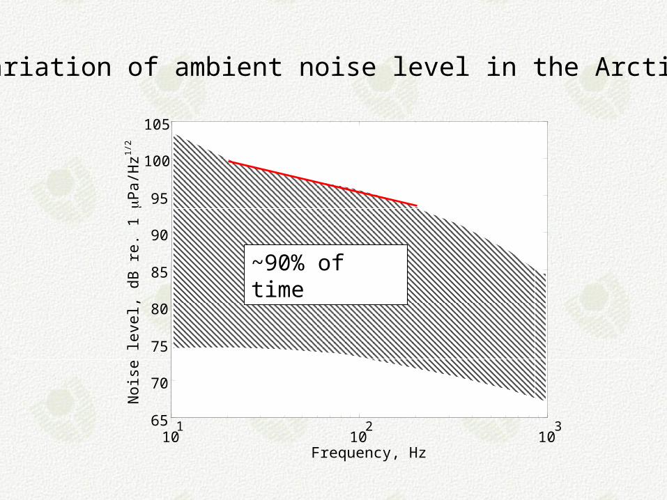
Variation of ambient noise level in the Arctic

101

102

10365

70

75

80

85

90

95

100

105

Frequency, Hz

Noi

se le

vel,

dB re

. 1

Pa/

Hz1/

2

~90% of time

10 1

10 2

10 -3

10 -2

10 -1

10 0

Frequency, Hz

Atte

nuat

ion,

dB

/km

F 1.5

Ice model parameters: mean ice thickness – 3.5 m; bottom standard deviation – 2.3 m; top standard deviation – 0.6 m; correlation length – 40 m

Frequency dependence of modes 1 - 40 attenuation modeled for the Central Arctic Basin and some experimental results

NUSC 1959

FRAM IV, 1982

TAP, 1994 (mode 1)

TAP, 1994 (modes 2-4)

ACOUS, APLIS (mode 1)

ACOUS, APLIS (mode 2)

Transmission loss along ACOUS path at 50 m and 400 m modeled for a broadband signal

0-dB SNR for a 50-Watt (~190 dB) source

Range, km200 400 600 800 1000 1200

30

40

50

60

70

80Depth: 400 m

-120

-115

-110

-100-95

-90

-140

-130

-120

-110

-100

-90

-80

-105

200 400 600 800 1000 1200

30

40

50

60

70

80-135

-130-125

-120

-115

-110

-105-100

-95

-90

-85

Range, km

Freq

uenc

y, H

z

Depth: 50 m

-20-dB SNR for a 50-Watt (~190 dB) source

Cabled/autonomous transceiver nodes

Cabled transceiver nodeswith shore terminals

Autonomous sources Acoustic observation pathsCable

90E

30

150

60

120

120

60

150

30

1800

GGGrrreeeeeennnlllaaannnddd

RRRuuussssssiiiaaa

CCCaaannnaaadddaaa

4000

500

35002000

500

500

2000

3500

2000

500

ACOUSsource

90WNotional acoustic network

1. Navigation:• Stationary acoustic sources are to transmit pulse-like signals

for accurate measurements of travel times to moving platforms. Nav. signals should also contain certain information (at least source ID numbers, UTC time, etc.).

3. Observation (thermometry, ice monitoring)Feasible for stationary receivers/transceivers. For mobile platforms, it requires accurate timing and complicated interpretation of travel time data.

2. Communication:• Two-way communication is needed to check the operational

state (most important) and to track position of mobile platforms

• Underwater communication of oceanographic data over long distances does seem feasible

) (),()( mss , t-kTS, t-iTS=tX dcc

))21(exp()(2)(1

0o

N-

i=isss c- jt-iTE = t, S c

c{ }c , c , ..., cN-0 1 1

dm m mN-m d , d , ..., d { }0 1 1

A simple method to design navigational/ communicational/observational signals

Series of two signals: training (observational) signals followed by informational signal = navigational signal

is the M-sequence of length N = 2M - 1

, where

, and

is the Hadamard code of number m < N

l

j=

M

i=

mijij

lm Syhy0 0

*0

)( Re=)(

Processing: compute the likelihood function:

for each message m, using Hadamard transform

Signal-to-noise ratio

10-1

1.0

0.0 0.05 0.10

0.15 0.20 0.25

M=512

M=1024

10-2

10-3

E

rror

pro

babi

lity

Error probability for binary message m at different SNR for two different signal bases

1. Weight, power consumption and reliability of low-frequency sources, especially for mobile platforms

Most serious problems

3. Slow communication rate

2. Doppler effect for mobile platforms

4. Accurate timing for mobile platforms

5. Separation of acoustic thermometry/halinometry data from navigational errors.

6,7,… ?