FILE CARVING AND MALWARE IDENTIFICATION ALGORITHMS APPLIED

TO FIRMWARE REVERSE ENGINEERING

THESIS

Karl A. Sickendick, Captain, USAF

AFIT-ENG-13-M-46

DEPARTMENT OF THE AIR FORCEAIR UNIVERSITY

AIR FORCE INSTITUTE OF TECHNOLOGY

Wright-Patterson Air Force Base, Ohio

DISTRIBUTION STATEMENT A.APPROVED FOR PUBLIC RELEASE; DISTRIBUTION UNLIMITED

The views expressed in this thesis are those of the author and do not reflect the officialpolicy or position of the United States Air Force, the Department of Defense, or the UnitedStates Government.

This material is declared a work of the U.S. Government and is not subject to copyrightprotection in the United States.

AFIT-ENG-13-M-46

FILE CARVING AND MALWARE IDENTIFICATION ALGORITHMS APPLIED TO

FIRMWARE REVERSE ENGINEERING

THESIS

Presented to the Faculty

Department of Electrical and Computer Engineering

Graduate School of Engineering and Management

Air Force Insitute of Technology

Air University

Air Education and Training Command

in Partial Fulfillment of the Requirements for the

Degree of Master of Science in Computer Science

Karl A. Sickendick, B.S.E.E.

Captain, USAF

March 2013

DISTRIBUTION STATEMENT A.APPROVED FOR PUBLIC RELEASE; DISTRIBUTION UNLIMITED

AFIT-ENG-13-M-46

FILE CARVING AND MALWARE IDENTIFICATION ALGORITHMS APPLIED TO

FIRMWARE REVERSE ENGll"'EERII'\G

Karl A. Sickcndick. B.S.E.E. Captain, USAF

Approved:

Maj Thomas E. Dube, PhD (Chaim1an)

Maj Jo1 athan W. Butts, PhD (Member)

Zt- Fn. \3 Date

L..{ 1\!kr I '"3. Date

Date

AFIT-ENG-13-M-46Abstract

Modern society depends on critical infrastructure (CI) managed by Programmable

Logic Controllers (PLCs). PLCs depend on firmware, though firmware security

vulnerabilities and contents remain largely unexplored. Attackers are acquiring the

knowledge required to construct and install malicious firmware on CI. To the defender,

firmware reverse engineering is a critical, but tedious, process.

This thesis applies machine learning algorithms, from the file carving and malware

identification fields, to firmware reverse engineering, then characterizes the algorithms’

performance. This research describes a process to speed and simplify PLC firmware

analysis, and implements that process with the cross-platform Firmware Disassembly

System. The system partitions a firmware into segments, labels each segment with a file

type, determines the target architecture of code segments, then disassembles and performs

rudimentary analysis on the code segments. This research characterizes the performance

of file carving algorithms applied to the file type identification problem, and of malware

identification algorithms applied to the architecture identification problem.

This research discusses the system’s accuracy on a set of pseudo-firmwares. Of the

algorithms it considers, the combination of a byte-frequency file carving algorithm and a

support vector machine (SVM) algorithm using information gain (IG) for feature selection

achieve the best performance. That combination correctly identifies the file types of 57.4%

of non-code bytes, and the architectures of 85.3% of code bytes.

Finally, the system performs opcode frequency analysis on disassembly results. This

research analyzes the opcode frequencies of four common PLC processor architectures.

Opcode frequency analysis provides analysts a measure of disassembly correctness. This

research applies the Firmware Disassembly System to several real-world firmwares, and

discusses the contents.

iv

Table of Contents

Page

Abstract . . . . . . . . . . . . . . . . . . . . . . . . . . . . . . . . . . . . . . . . . iv

Table of Contents . . . . . . . . . . . . . . . . . . . . . . . . . . . . . . . . . . . . v

List of Figures . . . . . . . . . . . . . . . . . . . . . . . . . . . . . . . . . . . . . . vii

List of Tables . . . . . . . . . . . . . . . . . . . . . . . . . . . . . . . . . . . . . . viii

List of Acronyms . . . . . . . . . . . . . . . . . . . . . . . . . . . . . . . . . . . . x

1 Introduction . . . . . . . . . . . . . . . . . . . . . . . . . . . . . . . . . . . . . 11.1 Problem Description . . . . . . . . . . . . . . . . . . . . . . . . . . . . . 11.2 Purpose and Goals . . . . . . . . . . . . . . . . . . . . . . . . . . . . . . 21.3 Summary of Contributions and Organization . . . . . . . . . . . . . . . . . 3

2 Background . . . . . . . . . . . . . . . . . . . . . . . . . . . . . . . . . . . . . 52.1 SCADA . . . . . . . . . . . . . . . . . . . . . . . . . . . . . . . . . . . . 5

2.1.1 Monolithic Architecture . . . . . . . . . . . . . . . . . . . . . . . 62.1.2 Distributed Architecture . . . . . . . . . . . . . . . . . . . . . . . 62.1.3 Networked Architecture . . . . . . . . . . . . . . . . . . . . . . . 72.1.4 Network Composition . . . . . . . . . . . . . . . . . . . . . . . . 82.1.5 PLC Composition . . . . . . . . . . . . . . . . . . . . . . . . . . 82.1.6 Threats . . . . . . . . . . . . . . . . . . . . . . . . . . . . . . . . 102.1.7 Attacks . . . . . . . . . . . . . . . . . . . . . . . . . . . . . . . . 12

2.2 Firmware . . . . . . . . . . . . . . . . . . . . . . . . . . . . . . . . . . . 142.3 Related Research . . . . . . . . . . . . . . . . . . . . . . . . . . . . . . . 16

2.3.1 File Carving . . . . . . . . . . . . . . . . . . . . . . . . . . . . . 172.3.2 Code Classification . . . . . . . . . . . . . . . . . . . . . . . . . . 25

2.4 Statistical Measures . . . . . . . . . . . . . . . . . . . . . . . . . . . . . . 26

3 Methodology . . . . . . . . . . . . . . . . . . . . . . . . . . . . . . . . . . . . 293.1 Problem Definition . . . . . . . . . . . . . . . . . . . . . . . . . . . . . . 293.2 Approach . . . . . . . . . . . . . . . . . . . . . . . . . . . . . . . . . . . 293.3 System Boundaries . . . . . . . . . . . . . . . . . . . . . . . . . . . . . . 323.4 Workload . . . . . . . . . . . . . . . . . . . . . . . . . . . . . . . . . . . 333.5 Performance Metrics . . . . . . . . . . . . . . . . . . . . . . . . . . . . . 353.6 Experimental Design . . . . . . . . . . . . . . . . . . . . . . . . . . . . . 36

v

Page

3.7 System Implementation . . . . . . . . . . . . . . . . . . . . . . . . . . . . 373.8 Methodology Summary . . . . . . . . . . . . . . . . . . . . . . . . . . . . 38

4 Results and Analysis . . . . . . . . . . . . . . . . . . . . . . . . . . . . . . . . 394.1 File Segmenting Algorithms . . . . . . . . . . . . . . . . . . . . . . . . . 394.2 Classifier Analysis . . . . . . . . . . . . . . . . . . . . . . . . . . . . . . 44

4.2.1 Fileprints . . . . . . . . . . . . . . . . . . . . . . . . . . . . . . . 444.2.2 Statistical . . . . . . . . . . . . . . . . . . . . . . . . . . . . . . . 504.2.3 Normalized Compression Distance . . . . . . . . . . . . . . . . . . 514.2.4 Decision Tree . . . . . . . . . . . . . . . . . . . . . . . . . . . . . 53

4.3 Classifier Accuracies . . . . . . . . . . . . . . . . . . . . . . . . . . . . . 564.3.1 Fileprints . . . . . . . . . . . . . . . . . . . . . . . . . . . . . . . 564.3.2 File Statistics . . . . . . . . . . . . . . . . . . . . . . . . . . . . . 604.3.3 Normalized Compression Distance . . . . . . . . . . . . . . . . . . 624.3.4 Code Classifiers . . . . . . . . . . . . . . . . . . . . . . . . . . . 66

4.4 Whole Pipeline . . . . . . . . . . . . . . . . . . . . . . . . . . . . . . . . 674.5 Opcode Analysis . . . . . . . . . . . . . . . . . . . . . . . . . . . . . . . 704.6 Firmware Disassembly . . . . . . . . . . . . . . . . . . . . . . . . . . . . 74

4.6.1 PPC & ZLib - Firmware 99449204.bin . . . . . . . . . . . . . . 754.6.2 ARM & ZLib - Firmware PN-20028.bin . . . . . . . . . . . . . . 804.6.3 ARM Only . . . . . . . . . . . . . . . . . . . . . . . . . . . . . . 834.6.4 Strengths and Weaknesses . . . . . . . . . . . . . . . . . . . . . . 83

5 Conclusions . . . . . . . . . . . . . . . . . . . . . . . . . . . . . . . . . . . . . 855.1 Limitations . . . . . . . . . . . . . . . . . . . . . . . . . . . . . . . . . . 865.2 Future Work . . . . . . . . . . . . . . . . . . . . . . . . . . . . . . . . . . 87

Appendix A: Disassembly at Four Offsets . . . . . . . . . . . . . . . . . . . . . . . 90

Appendix B: Opcode Frequency Analysis . . . . . . . . . . . . . . . . . . . . . . . 99

Bibliography . . . . . . . . . . . . . . . . . . . . . . . . . . . . . . . . . . . . . . 117

vi

List of Figures

Figure Page

2.1 Example SCADA network diagram . . . . . . . . . . . . . . . . . . . . . . . . 9

3.1 Block diagram of the Firmware Disassembly System . . . . . . . . . . . . . . 30

3.2 Firmware Disassembly System boundaries, inputs, and outputs . . . . . . . . . 32

4.1 File segmenter performance . . . . . . . . . . . . . . . . . . . . . . . . . . . 40

4.2 Fileprint of random files . . . . . . . . . . . . . . . . . . . . . . . . . . . . . 46

4.3 Fileprint of GZip training files . . . . . . . . . . . . . . . . . . . . . . . . . . 47

4.4 Fileprint of JPEG training files . . . . . . . . . . . . . . . . . . . . . . . . . . 47

4.5 Fileprint of Text training files . . . . . . . . . . . . . . . . . . . . . . . . . . . 48

4.6 Fileprint of PostScript training files . . . . . . . . . . . . . . . . . . . . . . . . 48

4.7 Fileprint of GIF training files . . . . . . . . . . . . . . . . . . . . . . . . . . . 49

4.8 Fileprint of code training files . . . . . . . . . . . . . . . . . . . . . . . . . . . 49

4.9 Statistical classifier model . . . . . . . . . . . . . . . . . . . . . . . . . . . . 50

4.10 Decision tree classifier model . . . . . . . . . . . . . . . . . . . . . . . . . . . 54

4.11 Decision tree leaf use on the training set . . . . . . . . . . . . . . . . . . . . . 55

4.12 Decision tree leaf use on the test set . . . . . . . . . . . . . . . . . . . . . . . 55

4.13 Proportions of opcode type . . . . . . . . . . . . . . . . . . . . . . . . . . . . 74

4.14 Symbol table contained in firmware 99449204.bin . . . . . . . . . . . . . . . 79

4.15 Code from the function UsrInit . . . . . . . . . . . . . . . . . . . . . . . . . 80

4.16 A portion of the IDA Pro code diagram for PN-20028.bin . . . . . . . . . . . 82

4.17 Summary of system performance on firmware 99449204.bin . . . . . . . . . 84

4.18 Summary of system performance on firmware PN-20028.bin . . . . . . . . . 84

vii

List of Tables

Table Page

1.1 Summary of contributions . . . . . . . . . . . . . . . . . . . . . . . . . . . . 4

2.1 Confusion matrix for a two-way classifier . . . . . . . . . . . . . . . . . . . . 26

2.2 Confusion matrix for an n-way classifier . . . . . . . . . . . . . . . . . . . . . 27

3.1 Characteristics of the test and training set file corpus . . . . . . . . . . . . . . 34

4.1 Performance vs. parameter value for the sliding window algorithms . . . . . . 42

4.2 Performance vs. parameter value for the entropy algorithms . . . . . . . . . . . 43

4.3 Training set characteristics . . . . . . . . . . . . . . . . . . . . . . . . . . . . 45

4.4 NCD classifier training corpus model statistics . . . . . . . . . . . . . . . . . . 52

4.5 Decision tree leaf use on the test and training set . . . . . . . . . . . . . . . . . 56

4.6 Test set characteristics . . . . . . . . . . . . . . . . . . . . . . . . . . . . . . 57

4.7 Producer accuracy confusion matrix for the Fileprints classifier . . . . . . . . . 58

4.8 Consumer accuracy confusion matrix for the Fileprints classifier . . . . . . . . 59

4.9 Fileprints classifier error summary . . . . . . . . . . . . . . . . . . . . . . . . 60

4.10 Producer accuracy confusion matrix for the file statistics classifier . . . . . . . 61

4.11 Consumer accuracy confusion matrix for the file statistics classifier . . . . . . . 62

4.12 File statistics classifier error summary . . . . . . . . . . . . . . . . . . . . . . 63

4.13 Producer accuracy confusion matrix for the NCD classifier . . . . . . . . . . . 64

4.14 Consumer accuracy confusion matrix for the NCD classifier . . . . . . . . . . 65

4.15 NCD classifier error summary . . . . . . . . . . . . . . . . . . . . . . . . . . 66

4.16 Code classifier omission and commission errors . . . . . . . . . . . . . . . . . 67

4.17 Overall accuracy summary, and 95% confidence interval . . . . . . . . . . . . 68

4.18 Producer accuracy summary by file type, and 95% confidence interval . . . . . 69

4.19 Most frequent opcodes from four architectures . . . . . . . . . . . . . . . . . . 71

viii

Table Page

4.20 Categorization of firmware contents . . . . . . . . . . . . . . . . . . . . . . . 75

4.21 Summary of Foremost output for the firmware . . . . . . . . . . . . . . . . . . 76

4.22 Contents of firmware 99449204.bin . . . . . . . . . . . . . . . . . . . . . . 78

4.23 Contents of firmware PN-20028.bin . . . . . . . . . . . . . . . . . . . . . . 81

A.1 Offset zero disassembly . . . . . . . . . . . . . . . . . . . . . . . . . . . . . . 91

A.2 Offset one disassembly . . . . . . . . . . . . . . . . . . . . . . . . . . . . . . 92

A.3 Offset two disassembly . . . . . . . . . . . . . . . . . . . . . . . . . . . . . . 93

A.4 Offset three disassembly . . . . . . . . . . . . . . . . . . . . . . . . . . . . . 94

A.5 Offset zero opcode analysis . . . . . . . . . . . . . . . . . . . . . . . . . . . . 95

A.6 Offset one opcode analysis . . . . . . . . . . . . . . . . . . . . . . . . . . . . 96

A.7 Offset two opcode analysis . . . . . . . . . . . . . . . . . . . . . . . . . . . . 97

A.8 Offset three opcode analysis . . . . . . . . . . . . . . . . . . . . . . . . . . . 98

B.1 Top 100 opcodes for ARM . . . . . . . . . . . . . . . . . . . . . . . . . . . . 99

B.2 Top 100 opcodes for Motorola 68000 . . . . . . . . . . . . . . . . . . . . . . . 103

B.3 Top 100 opcodes for PowerPC . . . . . . . . . . . . . . . . . . . . . . . . . . 107

B.4 Top 100 opcodes for AVR . . . . . . . . . . . . . . . . . . . . . . . . . . . . 112

ix

List of Acronyms

Acronym Definition

APT advanced persistent threat

ASCII American Standard Code for Information Interchange

BMP bitmap

CE Compact Edition

CERT computer emergency response team

CI critical infrastructure

COTS commercial off-the-shelf

CPU central processing unit

DHS Department of Homeland Security

DNS Domain Name System

EDS electronic data sheet

EEPROM electrically erasable programmable read-only memory

ELF Executable and Linkable Format

EPROM erasable programmable read-only memory

FAT File Allocation Table

FTP File Transfer Protocol

GIF Graphics Interchange Format

GUI graphical user interface

HMI human-machine interface

HTML HyperText Markup Language

I/O input/output

ICMP Internet Control Message Protocol

ICS Industrial Control System

x

Acronym Definition

IEC International Electrotechnical Commission

IG information gain

IP Internet Protocol

JPEG Joint Photographic Experts Group

k-NN k-Nearest Neighbor

LAN local area network

LZMA Lempel-Ziv-Markov chain algorithm

LZW Lempel-Ziv-Welch

NCD normalized compression distance

NIC network interface card

NTSB National Transportation Safety Board

OS operating system

PC personal computer

PCA principal component analysis

PDD Presidential Decision Directive

PDF Portable Document Format

PLC Programmable Logic Controller

RAM random-access memory

RMSE root mean square error

RPC remote procedure call

RTU Remote Terminal Unit

SCADA Supervisory Control And Data Acquisition

SMTP Simple Mail Transfer Protocol

SNMP Simple Network Management Protocol

SVM support vector machine

xi

Acronym Definition

TI Texas Instruments

US United States

WAN wide area network

XML Extensible Markup Language

xii

FILE CARVING AND MALWARE IDENTIFICATION ALGORITHMS APPLIED TO

FIRMWARE REVERSE ENGINEERING

1 Introduction

1.1 Problem Description

Programmable Logic Controllers (PLCs) quietly manage dozens of systems that

modern society depends on every day. PLCs, in turn, depend on firmware. Firmware is a

black box to control system operators, as they have no control or knowledge of its contents.

Though largely ignored in the past, recent security research focuses on firmware [69–73].

Researchers now routinely find remotely-exploitable PLC firmware bugs.

Few published efforts reveal PLC internals. Schwartz et al. focus on the

hardware internals [58], Peck and Peterson manually reverse engineer two firmwares but

their discussion does not focus on firmware contents [48], and McMinn considers the

communications protocols PLCs use to update firmware [41]. Manufacturers consider

many specifications proprietary, including processor architecture, and in most cases devices

are too expensive or mission critical to disassemble.

The networked generation of Industrial Control System (ICS) hardware enables

operators to make economic decisions which compromise system security. Operators

connect their critical infrastructure (CI) systems to their business networks to enable

improved customer service or less expensive long distance control. Attacking ICSs once

required a sophisticated, well-financed attacker. Recent high-profile incidents, like that

which pr0f srs claimed in 2011, show that ICS attacks no longer require many resources

[53]. More sophisticated attacks like Stuxnet now target PLCs specifically, but have

not yet attacked or modified PLC firmware [11]. History shows that these attacks are

1

likely coming. Open-source firmware projects for wireless routers [45, 63] and music

players [64], and published modifications of other firmware [19, 43], indicate that even

unsophisticated attackers will perpetrate PLC firmware attacks.

Once a system operator discovers that an attacker compromised their device, they

must determine the extent and effect of that compromise. Analysis requires a measure

of firmware reverse engineering. Unfortunately firmware is a black box to the user and

a proprietary, undocumented, binary blob to the researcher. Header format is arbitrary,

and varies between manufacturer and even model. Devices may reorder or uncompress

sections at several times, and may load code segments with arbitrary offsets. Devices

may skip installing firmware sections based upon hardware configuration. These device

activities complicate analysis, because firmware images retrieved with chip debugging tools

differ from pristine firmware images. Fortunately, manufacturers do not seem to purposely

obfuscate firmwares.

1.2 Purpose and Goals

The reverse engineering process is tedious [3]. It requires detailed analysis even

before disassembling code segments. Consequently, few analyses of PLC firmwares

exist, academic or otherwise. This research effort’s goal is to automate firmware reverse

engineering. Specifically, this research automates the steps of reverse engineering prior to

code analysis. It characterizes the performance of file carving and malware identification

algorithms when applied to firmware reverse engineering. This paper describes the

steps of firmware reversing, describes an implementation of those steps in the Firmware

Disassembly System, characterizes the system’s performance, and presents some PLC

firmware disassembly results.

Until recently, little need existed for efficient PLC firmware reverse engineering.

Forensics teams did not require the capability, and researchers had luck discovering

security vulnerabilities with externally-applied techniques like fuzzing [16]. Slow reverse

2

engineering methods sufficed for the patient researcher. This requirement changed with the

proliferation of Internet connectivity for attackers and CI alike.

The Firmware Disassembly System simplifies firmware reverse engineering. Firm-

wares often include compressed segments [48], and the system finds and uncompresses

those. Complex firmwares often include web-server functionality including documenta-

tion or status outputs, so the system identifies likely data segments containing common

file types. The Firmware Disassembly System finds segments containing executable code,

identifies the target architecture and disassembles that code, then performs rudimentary

analysis on the result.

This research hypothesizes that of the three file type identification algorithms it

considers, Axelsson’s normalized compression distance (NCD) algorithm provides the

most accurate type identification [7]. Axelsson’s experimental configuration involves more

file types than the other researchers’, and his n-valued classification results showed greater

accuracy, for several file types, than the other algorithms.

Of the two code segment architecture classification algorithms this research considers,

it hypothesizes that Kolter and Maloof’s boosted decision tree algorithm provides the most

accurate architecture and endianness detection [35]. In three out of four experimental

configurations, boosted decision trees provide the most accurate malware classification.

In the fourth configuration boosted decision trees provide the second most accurate

classification. support vector machines (SVMs) produce the second most accurate

classification when averaged over the four configurations.

1.3 Summary of Contributions and Organization

Table 1.1 summarizes this research’s contributions. Chapter 2 discusses the security

problems that motivate this research, and related work. Next, Chapter 3 concerns testing

methodology and system implementation. Chapter 4 discusses test results, and investigates

the reason for those results. Finally, Chapter 5 provides closing discussion.

3

Table 1.1: Summary of contributions

Contribution Relevant Section Related Work

Survey of related work Chapter 2 Academic: [9, 46]

Pseudo-firmware construction method Section 3.4

Firmware disassembly toolkit

construction

Section 3.7

Evaluation of file segmenting algorithms Section 4.1 Academic: [15, 33,

44]

File carving algorithm application to

firmware, and evaluation

Section 4.3 Academic: [5, 7,

12, 15, 23, 32, 33,

36, 38, 40, 44, 52,

60, 67, 74, 80]

Non-academic: [81]

Evaluation of malware classification

algorithm applied to

architecture-classification problem

Section 4.3 Academic: [35]

Opcode frequency analysis Section 4.5

PLC firmware content analysis Section 4.6 Academic: [18, 25,

79]

Non-academic: [19,

28, 29, 43]

4

2 Background

This chapter provides an overview of Supervisory Control And Data Acquisition

(SCADA) technology and its components. It discusses existing threats to SCADA

infrastructure, then discusses known and theoretical attacks against SCADA. The chapter

then provides a basic overview of device firmware. It considers firmware’s function and

complexity, then discusses firmware attacks. Finally, this chapter provides an overview of

related research including firmware analysis in other fields, research into file carving, and

compiled code architecture classification efforts.

2.1 SCADA

SCADA systems, and more generally ICS networks, control and monitor a diverse set

of modern industrial processes. Services including gas and electricity distribution, water

and wastewater control, telecommunications, and food processing rely on these systems to

provide a modern level of performance [8]. These processes are too complex to monitor and

control economically without automation techniques. SCADA and ICS systems make these

processes feasible by gathering data from remote sites, then correlating and displaying it at

an operator terminal. SCADA systems first came into prominence in the 1960’s and have

since evolved, along with computing itself [39].

SCADA systems are a part of the United States CI as Presidential Decision Directive

(PDD)-63 defined in 1998 [13]. CI includes public and private “physical and cyber-

based systems essential to the minimum operations of the economy and government”.

The directive acknowledges that in the past these systems were separate and independent,

but recent automation and interconnection introduced vulnerabilities. PDD-63, and the

Homeland Security Presidential Directive-7 in 2003 [10], establish United States (US)

5

policy regarding CI security. This section describes changes in SCADA infrastructure over

the years, and their motivation.

2.1.1 Monolithic Architecture

Initially, SCADA systems worked independently and in isolation, in a configuration

similar to server mainframes. These characteristics defined the monolithic phase of

SCADA architecture because one central unit, the SCADA Master, provided all computing

and monitoring functionality [39].

The lack of widespread networks and networking standards required every manufac-

turer to develop a proprietary system. Generally, the protocols did not tolerate other net-

work traffic and were not easily extensible. Manufacturers designed and installed each

SCADA system uniquely. The proprietary nature of the system software, networking, and

even the connectors, required the manufacturer to perform most system modifications.

Monolithic systems provided fault tolerance through SCADA Master redundancy. A

secondary system duplicated all functions of the primary, and monitored the primary’s

operation. When the secondary detected a fault it took over all operations. In general, the

secondary greatly increased system cost but performed little work.

2.1.2 Distributed Architecture

In the late 1980’s personal computers became more affordable, and local area network

(LAN) protocols became more standardized. These changes enabled SCADA architectures

that distributed operator functionality and processing across multiple systems. Individual

computers acted as human-machine interface (HMI) stations, as historian computers, and

in many other roles [39].

While manufacturers used standard LAN technologies to connect operator stations,

these networks had limited range. Many industrial processes still required communications

between geographically scattered equipment. Manufacturers continued to use proprietary

6

protocols developed during the monolithic architecture phase, and their makeshift wide

area networks (WANs) were effectively single-use.

Distributed architecture SCADA systems only contained vendor-provided equipment.

Often, only the vendor could perform system maintenance and upgrades. The distributed

architecture enabled more flexible and economical fault tolerance, however. Often, other

system components could handle the operations of failed system components in addition

to their own tasks. Thus, distributed architecture systems did not require full-time standby

systems.

2.1.3 Networked Architecture

Finally, in the mid 1990’s manufacturers began to use largely commercial off-the-

shelf (COTS) networking hardware and computer systems. They began to standardize

protocols for end-devices like PLCs and Remote Terminal Units (RTUs), which enabled

protocol transport over standard WAN networks. Standard protocols enabled companies to

make in-house modifications to their SCADA networks, and to lower costs by leveraging

their existing network infrastructure [39].

The networked SCADA architecture gave organizations greater flexibility in their

operations. Connection with the business network for performance tracking and billing

purposes became simple [39]. Networked architectures also enabled off-site backup

and fault-tolerance, enabling systems with the ability to survive disasters affecting entire

geographical regions.

For all the benefits, the networked generation created new issues regarding system

security and reliability. Unexpected interaction between SCADA and business systems

caused reliability issues. Manufacturers’ use of standard network protocols lowered the bar

to system exploitation, and integrating CI and business network infrastructure expanded the

potential attack surface-area [39].

7

2.1.4 Network Composition

SCADA networks have a hierarchical structure, as Figure 2.1 shows. Sensors and

actuators comprise the lowest level, and the sensor network connects them to PLCs and

RTUs. Sensor network connections are generally short, and analog. PLCs and RTUs

consolidate control over the sensors and actuators, then SCADA master units control the

PLCs and RTUs via the field network. Field networks consist of longer-distance links than

the sensor network. Modern field networks consist of Ethernet, serial cable, microwave

radio, telephone, and many other connections [8].

The control centers provide centralized operator control over the system, and include

terminals such as HMIs and data historians. Respectively, these enable operator control

over a physical process, and long term system state storage. Modern control centers consist

of COTS computer and networking hardware, running COTS operating systems and custom

control software. For example, Siemens’ SIMATIC WinCC product supports several

operating systems, from Microsoft Windows XP through Windows 7 [59]. SIMATIC

WinCC is Siemens’ primary control system software product, and Siemens is one of the

largest ICS manufacturers [58].

Increasingly, companies connect control centers to their business networks. Generally

they make this connection through a COTS firewall. Business network connections

enable companies to manage expenses and billing in real time, and to save costs by

leveraging existing long-distance network connections. These connections also introduce

vulnerabilities into the control system because many business networks have connections

to external networks like the Internet.

2.1.5 PLC Composition

The general PLC hardware architecture is modular, with some PLCs permitting end-

user module configuration, and others permitting only manufacturer configuration [58].

Modules communicate via the backplane and include processor, communications, and

8

Figure 2.1: Example SCADA network diagram

input/output (I/O) modules. The processor module executes ladder-logic code to manage

physical processes, coordinates between the other modules, and even handles simple field

network communications if the PLC does not include a communications module. As such,

the processor module is generally the most complex.

The communications module is of similar complexity to the processor. The module

handles time-sensitive network communications, and frees the processor module to manage

9

time-sensitive physical processes [58]. Communications modules handle multiple types of

network communications, including Internet Protocol (IP) over Ethernet and RS-422.

I/O modules output and input analog signals based upon commands from the processor

module [58]. These modules read gauges and switch positions, and control motors and

solenoids. I/O modules require the least intelligence, as their function is to process simple

backplane commands and manage digital/analog conversion hardware.

All three PLC modules contain microprocessors, and the most common processor

architectures are ARM, Motorola 68000 and PowerPC [58]. The processors execute code

contained in PLC firmware, and generally stored in nonvolatile flash memory. Additionally,

the processors interpret operator instructions regarding physical processes. Proprietary

software derives the instructions from one of the simple programming languages defined in

International Electrotechnical Commission (IEC) 61131-3 [31]. The specification defines

the Ladder Diagram, Function Block Diagram, Structured Text, and Instruction List

languages. Operators commonly call instructions in these languages ladder-logic.

2.1.6 Threats

The Department of Homeland Security (DHS) defines five groups of cyber threats,

depicted below in order of increasing consequence and decreasing threat frequency [17].

Nuisance hackers comprise the overwhelming majority of cyber attacks and include groups

such as hacktivists, individuals that use cyber action as a form of protest or to achieve

political ends [56]. Despite the group’s lack of resources and the general low complexity of

their attacks, nuisance hacker attacks occasionally cause significant economic consequence

[42]. Notoriety, mischief, or publicity for a cause frequently motivate nuisance hackers.

Money motivates criminals and gangs, who have resources which enable attacks of greater

complexity than nuisance hackers. The DHS list of cyber threats is:

1. Nuisance Hackers

2. Criminals and Gangs

10

3. Nation-States Motivated by Theft

4. Limited Resource Nation-States and Terrorists

5. Unlimited Resource Nation-States

Threat groups three through five possess significantly more resources [17]. Each has

the ability to seize control, through force, of corporations which produce cyber technology.

Military concerns motivate each, and economic and diplomatic concerns motivate all but

terrorists. Group three includes nation-states that steal private intellectual property and

national secrets. This threat group’s actors are unwilling to cause physical damage with

their actions, though they possess that capability. The limited and unlimited resource

groups are willing to cause physical damage. Money, time, or technical access may limit

the limited resource actors. Unlimited resource actors attack with monetary resources,

technical access, and speed, that overwhelm any adversary.

Attacks on the older, distributed architecture, SCADA systems, require physical

access and special network equipment. These requirements demand a moderate amount

of attacker resources. Attacks demand long-term planning, and that reduces attack payoff.

Modern networked SCADA systems lower the bar to attacker entry. Their connections

to the Internet, and use of common network protocols, enable nuisance hacker attacks.

Search engines like SHODAN make searching for Internet-facing SCADA networks simple

[68]. SHODAN and tools like Metasploit and THC-Hydra enable nuisance hacker

SCADA HMI attacks.

System operators can recognize many simple cyber attacks by their immediate system

effects, but the term advanced persistent threat (APT) describes a more insidious attacker

[66]. Long term reconnaissance and data exfiltration characterize the APT. These

actions require more resources than nuisance hackers possess, and until recently required

11

more resources than criminals possessed. The proliferation of network attack tools and

knowledge enables organized criminals to act as APTs.

The insider threat and self-inflicted malfunction form a sixth threat category [62].

Insiders are employees and business associates that intentionally cause damage to an

organization. They work with an external actor, or alone, to sabotage the organization.

Insiders do not require many resources because their position grants them access to

critical systems. Separately, self-inflicted malfunction causes unintentional damage to an

organization, and occurs due to operator error or equipment failure.

Emergency responders found self-inflicted malfunction as the cause of several

SCADA emergencies, although attribution is notoriously difficult when an incident includes

cyber assets. The National Transportation Safety Board (NTSB) attributed a gasoline

pipeline leak in Bellingham, Washington, to pipeline damage and degraded SCADA

software performance [1]. The leak and a subsequent explosion resulted in three deaths.

Investigators were unable to determine the cause of the software performance degradation,

but determined that it was likely due to an administrator’s configuration update on the live

system. The investigators also found several network security issues that could have led to

the pipeline leak, leaving open the possibility of an intentional attack.

2.1.7 Attacks

Vitek Boden attacked the Maroochy Shire Council sewage system in 2000 in the

first well-known ICS attack [2]. He stole equipment from Hunter Watertech, his former

employer and the company which installed the SCADA system, then used the equipment

to sabotage the system’s operation. The system lacked cyber defenses, and its security

relied on the obscurity of the system’s radio communication frequencies and protocols.

Vitek disabled sewage pumps and sensor alarms, and disrupted remote station

communications at several locations over a period of three months [2]. Initially, operators

attributed malfunction to installation error. A lack of cyber defense logs and tools, and

12

Vitek’s actions to hide his attacks, led system operators to that incorrect conclusion. Vitek’s

success was due to his theft of equipment and a lack of cyber defense, and as such his attack

was of low complexity.

Attacker pr0f srs broke into the water infrastructure for South Houston, Texas, in 2011

[53]. He claimed that the SCADA system used a three letter password, and that knowledge

of the system’s software, and guessing the password, allowed him control over the system.

The attacker posted screenshots of the control system to Twitter and claimed that the attack

was partly in response to public DHS statements [65]. This attack was of low complexity,

and the attacker acted as a hacktivist in this instance.

Stuxnet is a computer worm that targets particular ICS hardware configurations and

sabotages their operation [11]. Specifically, Stuxnet targets Siemens’ SIMATIC PCS 7, an

industrial automation system in which the operator terminals execute Microsoft Windows.

It uses four exploits to propagate: a Windows shortcut vulnerability, shared network

folders, a Windows remote procedure call (RPC) vulnerability, and a Windows printer

sharing vulnerability [37]. Stuxnet uses several other Windows vulnerabilities to increase

its privileges.

Stuxnet modifies code on PLCs to vary the speed of motors [24]. The modified motor

speed sabotages the industrial process controlled by the motor. Some researchers count

Stuxnet among the most complex threats they have analyzed. It exploits at least four

previously-undisclosed bugs, and analysis shows that an organized team with delineated

responsibilities likely built its components [37]. Analysts believe that constructing the

Stuxnet worm required resources beyond the capabilities of all but a few attackers [24].

The complexity and consequences of Stuxnet suggest that the attacker belonged to threat

groups four or five: limited resource nation-states and terrorists, or unlimited resource

nation-states.

13

2.2 Firmware

Firmware exists on the boundary of hardware and software. Firmware controls

the start-up sequence of modern personal computers (PCs), enabling low-level user

configuration and transfer to larger, more complex operating systems (OSs). Firmware

eases startup by permitting modern OSs access to a standard interface, abstracting out

many differences in PC hardware. Modern PCs store firmware in electrically erasable

programmable read-only memory (EEPROM) chips, and store the main OS on storage

external to the system motherboard.

In contrast, firmware often provides all system software functionality for embedded

devices. Due to space and durability requirements embedded devices often do not contain

storage external to the motherboard, and can therefore only execute an OS stored in

EEPROM or flash memory. Little reason exists, then, for firmware to transfer control to

any other entity, and manufacturers incorporate a full OS and all software in the firmware.

Generally, PC OSs and software provide simple update techniques, enabling users to

patch insecure software quickly once manufacturers release updates. Updates to firmware

require more user effort. Many systems require that the user reboot into maintenance

mode or manipulate hardware switches. Performance or safety-critical devices may require

disconnection from the rest of the system. Firmware’s critical function also makes testing

procedures more vital than for conventional software. These complications make firmware

security vulnerabilities more valuable to attackers.

Dacosta et al. reverse engineer the firmware of a Cisco 7960G IP phone [18]. They

first disassemble the binary firmware image, retrieving the assembly code for the phone’s

ARM processor. Then they manually perform control and data flow analysis to look for

potential software vulnerabilities. Firmware image disassembly requires several steps.

First, the researchers note that the firmware image consists of a compressed ZIP archive

14

containing five named files. They deduce the contents of the files, then character strings

within the files identify the phone processor’s architecture.

Once they determine the code’s target architecture, the researchers possess much of

the information they require for code disassembly. Dacosta et al. manually analyze and

determine the contents of the file headers. They disassemble the appropriate code sections

and analyze addresses in switch statement jump tables to determine the code’s memory

mapping. The researchers identify C library functions that commonly lead to security

vulnerabilities, including strcpy, malloc, and sprintf, then begin manual code analysis

from those points.

Critically, Dacosta et al. note that they are not aware of tools that automate analysis

of ARM binaries. They use IDA Pro to perform the majority of their analysis. They use

their intuition to perform the initial analysis of the binary firmware image. They have

success relying on standard compression tools to unpack most of the image, and relying on

character strings to reveal the target architecture.

Delugre analyzes and modifies the firmware for a Broadcom Ethernet network

interface card (NIC) [19]. The Linux kernel contains the binary firmware image in an

undocumented format. Delugre determines that the firmware targets a MIPS processor

by locating the central processing unit (CPU) model on the physical device. He uses a

modified Linux kernel driver to retrieve the firmware from the NIC while in operation. The

process reveals the relevant memory addresses for code analysis and disassembly. After

retrieving the NIC firmware code, Delugre discusses how to compile and install firmware

with covert communications capabilities.

Miller disassembles the firmware of an Apple MacBook smart battery [43]. He

destructively disassembles the hardware to determine its components. The researcher

removes the Texas Instruments (TI) chips containing the firmware and uses TI software

to retrieve the firmware image. Miller manually analyzes the firmware contents and,

15

although TI holds the firmware’s target architecture as proprietary information, the

researcher determines the target architecture from the format of several instructions. Miller

successfully modifies the battery firmware to report incorrect values for battery capacity

and charge.

Yasinsac et al. analyze the security of voting machine firmware [79]. They use

static code analysis and manual code review to find vulnerabilities in Florida voting

machines. The machines contain external storage (Compact Flash and a proprietary voting

ballot device) and on-board flash memory. An erasable programmable read-only memory

(EPROM) chip contains the voting machine firmware, but the manufacturer provides the

researchers with the firmware source code. The firmware contains all application code, and

was written entirely by the vendor, with the exception of the Compact Flash driver and C

standard library. Yasinsac’s review finds several buffer overflow vulnerabilities, and the

researchers theorize about potential problems with the general voting security process.

Fogie applies firmware reverse engineering techniques to Windows Compact Edition

(CE) embedded systems [25]. He discusses the basics of the ARM architecture, and

applies several common reverse engineering tools to real firmware. Hurman goes into

similar detail about Windows CE, but focuses on exploiting bugs and crafting shellcode

[29]. His analysis discusses embedded system software analysis using reverse engineering

techniques. Grand discusses general security concerns regarding firmware code, and

suggests that manufacturers incorporate code signing and encryption [28]. He notes that

they can immediately increase security by removing firmware images from public websites.

Grand also points out that manufacturers can use obfuscation to discourage the majority of

attackers.

2.3 Related Research

This research effort develops techniques to automate the firmware analysis process.

No known research considers firmware analysis as a rigorous process, but some research

16

analyzes embedded system firmware, and the individual activities required for firmware

disassembly are active areas of research.

Peck and Peterson perform some related work in [48], where they disassemble the

firmwares for two PLC Ethernet modules. The authors separate program code from

the Rockwell 1756 ENBT and Koyo H4-ECOM100 Ethernet module firmwares, then

demonstrate a proof-of-concept modification of the Rockwell firmware. They place their

firmware modification within the firmware’s File Transfer Protocol (FTP) server code, and

program it to send an Internet Control Message Protocol (ICMP) ping to a remote host

periodically. The authors update a target PLC over an Ethernet network, and find that the

PLC performs no authentication of the firmware code or of the personnel performing the

firmware update. Both devices update firmware over custom protocols, and current COTS

firewalls do not understand those protocols. In addition to the firmware modification, the

authors demonstrate cross-site scripting attacks on both Ethernet modules’ web servers.

The Rockwell device also provides FTP and Simple Network Management Protocol

(SNMP) servers, and both servers have authentication vulnerabilities.

With their paper, Peck and Peterson demonstrate that malicious firmware modification

and installation, while not simple, is within the realm of the determined hacker. They

outline several situations where this form of attack benefits the attacker. The authors

conclude that system operators must be vigilant with PLC network security. Ultimately, the

proprietary nature of PLC firmware requires that vendors take action to improve security.

SCADA asset owners must hold vendors accountable by taking security into account when

purchasing equipment.

2.3.1 File Carving

Firmware images contain many component segments, including code and data

segments. Separating data from code is an initial step in firmware disassembly. File

carving is an active area of research in the digital forensics field that involves identifying

17

and recovering files from hard disks, including partially destroyed disks. File carving

techniques are applicable to firmware image disassembly, and this section describes several

file carving research efforts.

Traditional file carvers search for file magic numbers, sequences of bytes that identify

the headers or footers of particular file types. The UNIX file command has existed since

at least 1973, and is the most well-known example of anything like a traditional file carver

[81]. The file command has a flexible configuration file which specifies magic numbers

for hundreds of file types. In general, it does not search for multiple sections and file types

within a file.

Foremost searches for magic numbers in both headers and footers, and carves the

appropriate section [46]. The United States Air Force Office of Special Investigations

developed the tool, and it is now an open-source project. Its configuration file allows users

to specify new file types by adding the header and footer magic numbers. Scalpel is a

traditional file carver Richard et al. designed for high performance [52]. Richard outlines

requirements for a high performance file carver, and implements those requirements by

improving Foremost.

Sites et al. describe a system for binary code translation between two architectures

[60]. The system locates the code within an executable, then translates it for a second

architecture. An executable’s header and symbol table describe the entry points for much of

the code, but can skip some. Sites’ system attempts to find other code by scanning through

sections skipped by the header and symbol table, including groups of valid instructions

which end in an unconditional branch or jump.

Underwood extends context-free grammars to describe the format of binary files, and

validates a binary file’s format via a context-free grammar parser [67]. The technique can

detect file format more accurately than simple magic number detection, but requires much

18

more metadata describing each format. The technique is most useful for finding well-

formed files, or detecting which file parts are not well-formed.

McDaniel and Heydari first describe fingerprinting file types with byte frequency

analysis [40]. For each training file, their system generates an array of normalized

frequencies for each byte value. The system averages all files of a particular type, then

calculates a correlation strength similar to variance, to generate a fingerprint for that type.

The researchers create an algorithm to compute a test file’s similarity to each fingerprint,

then classify the test file’s type as that of the most similar fingerprint. Their test set contains

30 file types, and the classifier performs 30-class classification. When relying on file

headers and footers, their algorithm achieves a 96% accuracy. Otherwise, it achieves only

a 46% accuracy.

Erbacher and Mulholland distinguish file and data type to facilitate the identification of

compound file contents [23]. Compound files, like Microsoft Word Documents or firmware

images, can contain other files in addition to their own data and metadata. Thus while a

file’s overall file type may be Word Document it also contains other data types, like images

and spreadsheets, in their native file types. They apply 13 statistical file measures to a 7 file

type test corpus, and find that the measures which best differentiate the test files by type

are: average byte value, distribution of byte value averages, standard deviation, distribution

of standard deviations, and kurtosis.

Moody and Erbacher describe a system, SADI, which applies 6 statistical techniques

to data type identification [44]. Their techniques include distribution of byte values, and

Erbacher and Mulholland’s top five. They classify sections of test files using a sliding

window which varies by file type, but is generally 256 bytes. This enables them to identify

data types within a file. The system achieves 74% accuracy on 9-class classification.

In the Oscar file carver, Karresand and Shahmehri classify files with the normalized

Euclidean distance to a file type centroid [33]. Their file type centroids consist of the byte

19

value frequency mean and standard deviation of a set of files belonging to that type. The

researchers built Oscar to assist with hard disk analysis, so it classifies disk image sections

with a disk-cluster sized sliding window of 4 kB, with a 4 kB step size. Karresand’s test set

concatenates 49 file types, and Oscar classifies each cluster as Joint Photographic Experts

Group (JPEG) or not-JPEG. Oscar achieved a 98% true positive rate, 0.01% false positive

rate, on the two-way classification problem.

Later, the researchers expand Oscar to consider a byte value rate-of-change frequency

metric [32]. Their system calculates the absolute value of the distance between all

consecutive bytes, then builds a histogram with those values. The rate-of-change values

fall within the range 0 to 255. The system extends the original Oscar centroids with the

rate-of-change means and standard deviations. Karresand and Shahmehri use the same

distance metric for both byte value frequency and rate-of-change frequency centroids. With

the extended system, the researchers boost classification accuracy on the JPEG two-way

classification problem to a 99% true positive rate, 0% false positive rate.

Veenman uses a byte value histogram, entropy, and Kolmogorov complexity with

a linear classifier to classify files [74]. His research considers both 2- and 11-class

classification problems, over 11 file types. The use case in Veenman’s research is digital

forensics, thus his file corpus included common desktop file types. Veenman achieved the

best accuracy, a 45% true positive rate, with 2-class classification.

Mayer applies long byte value n-grams, for 2 ≤ n ≤ 20, to file type classification [38].

His research considers 25 file types common to office environments, and models file types

with the long n-grams common to that type. To each test sample, the classifier assigns the

file type that maximizes the number of common n-grams present. Mayer achieves a 48%

accuracy on full files and a 22% accuracy on file segments. This large accuracy difference is

due to his exclusion of file headers from the segments, but the inclusion of header n-grams

in his file type models.

20

Amirani et al. apply principal component analysis (PCA) to extract classification

features from the byte frequency distribution of test files [5]. They use the resulting

features to train a neural network to classify files of 6 types. The neural network allows

the researchers to achieve accurate classification, while PCA reduces the network size and

training time. They classify Microsoft Word, Windows Executable, Portable Document

Format (PDF), JPEG, HyperText Markup Language (HTML), and Graphics Interchange

Format (GIF) files. The system achieves an overall accuracy of 98% when classifying file

fragments that do not include headers or footers.

Calhoun and Coles perform 2-class file segment classification using Fisher’s linear

discriminant with 11 data statistics and 5 combinations of those statistics [12]. Their data

statistics include: entropy, mean byte value, byte value standard deviation, correlation,

longest common subsequence length, and byte value frequencies for bytes within a range.

While their research only quantifies results of 2-class classification, they state that their

technique applies to the more general n-value classification problem

Calhoun and Coles test their technique with two sets of GIF, JPEG and bitmap (BMP)

files. The first set includes bytes 128 through 1024 of each file, and the second set includes

bytes 512 through 1024. Including only part of each file enables them to test the accuracy

of their technique when files do not include metadata, and when forensic investigators have

only partially recovered a file. The statistic which performs best on the first test set is a

combination of byte frequency over three ranges, entropy, byte frequency mode, and byte

frequency standard deviation. This combination achieves 88.3% accuracy on the first set

and 84.2% accuracy on the second. Longest common subsequence yields the best accuracy

on the second set, at 86%, and 84.5% accuracy on the first set.

Axelsson uses NCD and k-Nearest Neighbor (k-NN) to perform n-value file segment

classification [7]. NCD is an approximation of normalized information distance, which

is a measure of data entropy. Axelsson defines NCD with Equation 2.1, where C(x) is

21

the compressed length of x, and C(x, y) the compressed length of x and y concatenated.

He chooses gzip as the compression algorithm, and investigates settings of k from 1 to

10. The algorithm calculates NCD for 512 B test and training fragments, then assigns test

segments the most common file type among the k lowest NCD values.

NCD(x, y) =C(x, y) −min(C(x),C(y))

max(C(x),C(y))(2.1)

Axelsson’s file corpus contains 17 file types including executable files, images,

movies, and common document formats. He reports approximately 50% accuracy overall

for the 17-value classification problem, but approximately 90% accuracy for several file

types. Furthermore he finds that, among the tested values, no k value performed better than

the others. Axelsson suggests that future work should consider classifying fragments into

more generic file type classes.

Conti et al. classify 14,000 1 kB file fragments from 14 common file types using k-NN

[15]. Their k-NN algorithm evaluates the distance between fragments with Euclidean and

Manhattan distance over 4 file statistics: Shannon entropy using byte bigrams, byte value

arithmetic mean, Chi Square Goodness of Fit of byte distribution to a random distribution,

and Hamming weight. They define Hamming weight as the proportion of one bits in a

segment. Equations 2.2 and 2.3 give the Shannon entropy and Chi Square equations,

respectively. In Equation 2.2, p(Xi) represents the probability that byte value i occurs

within a file fragment. In Equation 2.3, oi represents the frequency of byte i within a

file fragment, and ei represents the expected frequency of byte i within a uniform random

distribution. Conti et al. calculate Chi Square Goodness of Fit using the χ2 value and a Chi

Square distribution with 255 degrees of freedom. They determine that, for their test cases,

Euclidean distance classifies file fragments more accurately than Manhattan distance.

22

H(x) = −

255∑i=0

p(Xi)log10(p(Xi)) (2.2)

χ2 =

255∑i=0

(oi − ei)2/ei (2.3)

They extract file fragments from the approximate middle of sample files to avoid file

headers and footers. Their 14 file types consist of compressed data in several formats,

encrypted data, random data, base64 or uuencoded data, Linux ELF and Windows PE

executable data, bitmap data, and mixed text data. During classification, Conti et al.

test values of k from 1 to 25, and settle on k = 3 because larger values provide no

significant return. The classifier was unable to distinguish several file types during 14-value

classification, so Conti et al. clustered each file type by similarity, making the problem 6-

value classification. They clustered the random, encrypted and compressed data together,

clustered the executable formats, and placed the other file types in individual clusters. Their

classifier achieved 82.5% accuracy for bitmaps, and better than 96% accuracy for the 5

other clusters.

Li et al. describe the performance of a system they call Fileprints [36]. The

system models file types with the mean and standard deviation of byte value frequency.

Li et al. design Fileprints to handle byte value n-grams, but determine that 1-grams

are sufficiently complex to accurately classify files. Additionally, a 1-gram file footprint

(a fileprint) contains only 256 elements, whereas a 2-gram fileprint requires 256 times

the storage space. Li et al. find the 1-gram fileprint performance sufficient, especially

considering the low storage requirement advantages.

The Fileprints test corpus consists of five general file types: EXE (including DLL

files), GIF, JPEG, DOC (including Word, Powerpoint and Excel files), and PDF. Li et al.

consider three model types. Their single-centroid model combines each file type’s training

examples into one fileprint per type. A multi-centroid model consists of multiple models

23

for each file type. K-means clustering builds K fileprints per type. The third model type

uses individual training examples as fileprints. Therefore, if n training samples belong to

file type t, Fileprints assigns n models to file type t.

With both the single and multi-centroid models Fileprints finds average byte value

frequencies over all training examples, then calculates the Mahalanobis distance to training

samples to determine the closest training model. Li et al. give Mahalanobis distance as

Equation 2.4, where i is byte value. Values xi and σi are the mean frequency and standard

deviation, respectively, for i in the training examples. Then, yi represents i’s frequency in

the test sample. Li et al. use α as a smoothing factor, which becomes necessary when

the standard deviation is 0. Fileprints classifies a test sample as the type of the closest

training example. No standard deviation values exist for Fileprints’ third model type,

so Li et al. cannot use Mahalanobis distance, and use Manhattan distance instead.

D(x, y) =

n−1∑i=0

|xi − yi|

σi + α(2.4)

Fileprints’ accuracy on the five-way classification problem with the single-centroid

model is 82%. With the multi-centroid model and individual-example models they find

89.5% and 93.8% accuracy, respectively. Li et al. find better performance when they

truncate files. Truncation causes file header magic numbers to occupy a greater percentage

of the total file. Li et al. truncate test and training files to include only the first 20 bytes, then

apply Fileprints using the single-centroid model. This test achieves 98.9% accuracy.

Zhang and White apply a system similar to Fileprints to network traffic. They use

their system to detect executables in network traffic [80]. Their extension to Fileprints

examines traffic that represents only a portion of an executable. The researchers’ goal is

to use their system as an anomaly detection system sensor, and thus detect anomalous or

hidden executables in network traffic.

24

2.3.2 Code Classification

Kolter and Maloof construct a system which classifies Windows executables as

malicious or benign using a variety of machine learning techniques [35]. They experiment

with boosted and un-boosted decision trees, SVMs, instance-based learners, and naive

Bayes classifiers to determine the most effective technique for the classification problem.

Kolter and Maloof perform pilot studies to determine the number of attributes, n-gram size,

and number of bytes-per-gram that produce the most accurate results. They settle on 500

byte value 4-grams, and use these parameters for the remainder of their tests.

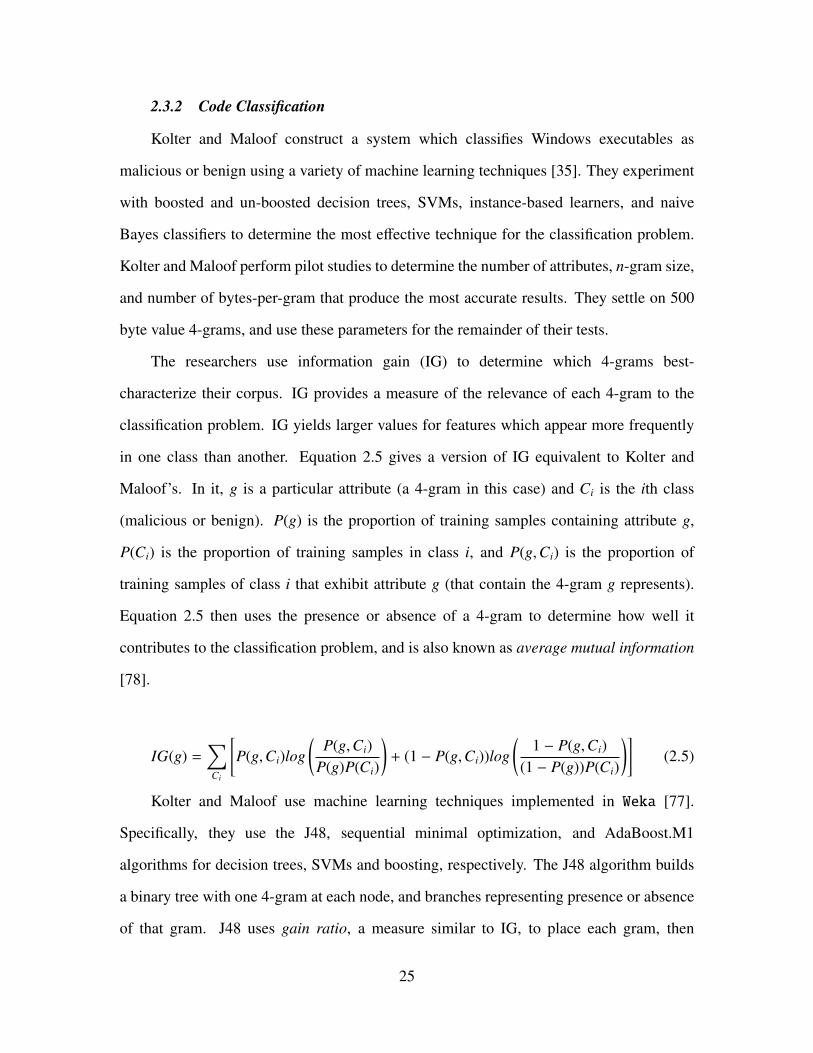
The researchers use information gain (IG) to determine which 4-grams best-

characterize their corpus. IG provides a measure of the relevance of each 4-gram to the

classification problem. IG yields larger values for features which appear more frequently

in one class than another. Equation 2.5 gives a version of IG equivalent to Kolter and

Maloof’s. In it, g is a particular attribute (a 4-gram in this case) and Ci is the ith class

(malicious or benign). P(g) is the proportion of training samples containing attribute g,

P(Ci) is the proportion of training samples in class i, and P(g,Ci) is the proportion of

training samples of class i that exhibit attribute g (that contain the 4-gram g represents).

Equation 2.5 then uses the presence or absence of a 4-gram to determine how well it

contributes to the classification problem, and is also known as average mutual information

[78].

IG(g) =∑Ci

[P(g,Ci)log

(P(g,Ci)

P(g)P(Ci)

)+ (1 − P(g,Ci))log

(1 − P(g,Ci)

(1 − P(g))P(Ci)

)](2.5)

Kolter and Maloof use machine learning techniques implemented in Weka [77].

Specifically, they use the J48, sequential minimal optimization, and AdaBoost.M1

algorithms for decision trees, SVMs and boosting, respectively. The J48 algorithm builds

a binary tree with one 4-gram at each node, and branches representing presence or absence

of that gram. J48 uses gain ratio, a measure similar to IG, to place each gram, then

25

prunes unhelpful branches to avoid overtraining [51]. Platt originally describes sequential

minimal optimization, a tool which makes training SVMs efficient [49]. The Weka

SVMs implementation solves multi-class problems through pairwise classification [77].

The AdaBoost algorithm boosts existing Weka classifiers by generating multiple classifier

models, then weighting them based on performance.

Kolter and Maloof apply their classification system to a corpus of 1,971 benign and

1,651 malicious Windows executables. They find that the boosted decision tree and SVM

classifiers perform best, with true positive rates exceeding 0.95 for false positive rates less

than 0.05.

2.4 Statistical Measures

Typical definitions of statistical measures such as true positive rate, false positive rate,

true negative rate and false negative rate work well for two-way classifiers. Equations 2.6,

2.7, 2.8, and 2.9 depict these measures, with values corresponding to the two-way classifier

confusion matrix in Table 2.1. General n-way classifiers require more general statistical

measures, and Equations 2.10, 2.11, 2.12, and 2.13 give these measures [61]. Values

correspond to the n-way classifier confusion matrix in Table 2.2.

Table 2.1: Confusion matrix for a two-way classifier

Prediction

negative positive

Act

ual

negative samplesn,n samplesn,p

positive samplesp,n samplesp,p

26

true positive rate =samplesp,p

samplesp,p + samplesp,n(2.6)

false negative rate =samplesp,n

samplesp,p + samplesp,n(2.7)

true negative rate =samplesn,n

samplesn,p + samplesn,n(2.8)

false positive rate =samplesn,p

samplesn,p + samplesn,n(2.9)

The true positive and true negative rate equations correspond with producer accuracy

in the case of a 2-way classifier. Likewise, the false positive and false negative rate

equations correspond with omission error. Producer accuracy is the percent of samples

of classi that the classifier identifies correctly as belonging to classi. It is the likelihood

that the classifier will identify an item correctly, given that it belongs to a specific class.

Consumer accuracy is the percent of samples the classifier identifies as classi that actually

belong to classi. It is the likelihood that a particular class’s output correctly identifies a

particular class.

Table 2.2: Confusion matrix for an n-way classifier

Prediction

class1 class2 ... classn

Act

ual

class1 samples1,1 samples1,2 ... samples1,n

class2 samples2,1 samples2,2 ... samples2,n

... ... ... ... ...

classn samplesn,1 samplesn,2 ... samplesn,n

27

class i producer accuracy: PAi =samplesi,i∑n

m=1 samplesi,m(2.10)

class i omission error: PEi =

∑nm=1 samplesi,m − samplesi,i∑n

m=1 samplesi,m= 1 − PAi (2.11)

class i consumer accuracy: CAi =samplesi,i∑n

m=1 samplesm,i(2.12)

class i commission error: CEi =

∑nm=1 samplesm,i − samplesi,i∑n

m=1 samplesm,i= 1 −CAi (2.13)

Equation 2.14 provides a rough measure of overall classifier accuracy. It yields the

total percent of correctly identified samples.

overall accuracy =

∑nm=1 samplesm,m∑

samples(2.14)

This chapter provided an overview of SCADA technology, describing system

components, current threats, and attacks. It discussed firmware’s function on PLCs,

and the potential for firmware-based attacks. This chapter provided an overview of

research related to this thesis, including work on firmware reversing, file carving, and

malware identification. Chapter 3 describes the file carving and malware identification

algorithms this research applies to firmware disassembly. It discusses this research’s

purpose and experimental methodology. Chapter 3 describes how this research assesses

those algorithms, how it eases firmware disassembly, and how the research validates its

results.

28

3 Methodology

3.1 Problem Definition

This research determines the effectiveness of a set of techniques which characterize,

disassemble, and analyze firmware. It seeks to automate firmware analysis whether the

vendor provides that firmware, an analyst forensically retrieves it from the contents of an

EEPROM, or a security professional intercepts it after malicious third party modification.

Therefore, the techniques this research develops must consider firmware in a generic sense.

The ideal technique set makes no assumptions about vendor firmware layout decisions or

header and footer contents. These parameters vary between vendors, devices, and firmware

acquisition method.

The analysis process begins by separating a firmware into likely component segments

and identifying the file types of those segments, then identifying the target architecture of

code segments. Therefore, this research focuses on techniques capable of completing these

two tasks. It evaluates three techniques which identify firmware file segments by file type,

and two techniques that identify code segment target architectures. This research seeks to

identify algorithms which provide the most accurate firmware segment decomposition and

code architecture classification.

3.2 Approach

Figure 3.1 depicts the system under test, the Firmware Disassembly System. To

disassemble firmware, a software system must uncompress compressed segments. It must

identify component segment boundaries, then identify those segments’ file type. The file

type classifier identifies some segments with the code file type, and the software system

must then classify those segments’ architecture and endianness. Finally it must disassemble

the binary code segments, resulting in correct assembly-language code output.

29

Figure 3.1: Block diagram of the Firmware Disassembly System

This research applies file carving algorithms to the file type identification problem, and

applies malware identification algorithms to the code architecture identification problem.

It evaluates each algorithm’s accuracy when applied to firmware binaries or code segments

respectively.

Each file carving algorithm classifies the file type of a segment of the binary image.

The file carving algorithms do not segment the file themselves, and require a separate

segmentation algorithm. This research considers two segmentation algorithms. Conti et

al. solve the problem of segmenting binary files with a sliding window [15]. The sliding

window is 1024 bytes wide with a step size of 512 bytes, and matches properties of their

statistical classifier. This research considers file segmentation with a generalized version

of the sliding window. The second file segmentation technique calculates an entropy value

for each byte in a firmware based on a sliding window. It uses a segmented-least-squares

algorithm to minimize the number of firmware sections, and to minimize the squared error

of each section’s mean entropy [34].

This research’s first file type identification technique is Axelsson’s [7]. He

characterizes files with NCD, then associates them with file types from the training set

using k-nearest neighbor. In the second technique, Li et al. perform n-gram analysis on

30

their training set to characterize file types, then use Mahalanobis distance to associate files

with file types [36]. The third file carving technique characterizes file segments with four

statistical signatures [15]. Conti et al. use k-nearest neighbor to associate members of their

test set with file types. All three file carving algorithms perform classification for two or

more classes.

Kolter and Maloof apply data mining techniques to malware detection and classifi-

cation [35]. They collect 4-grams from executables, rank them by information gain, then

select the top 500 as classifier attributes. They classify the resulting 4-gram set with seven

algorithms. Their best results come from the boosted decision tree and SVM algorithms.

This research uses the decision tree and SVM algorithms, with Kolter and Maloof’s at-

tribute selection technique, for code architecture identification.

Each algorithm requires a training set and a test set. The test and training sets

for the file carving algorithms consist of firmware images and sets of files common to

firmwares respectively. Training and test sets for the code classification algorithms consist

of code segments common to firmwares, as Section 3.4 describes. Metadata describes the

characteristics of each member in the test and training sets. The file carving algorithms

and the code classification algorithms use supervised training, so training samples require

metadata describing their file type, or code architecture and endianness. Testing the

pipeline as a whole requires firmwares or pseudo-firmwares, and metadata describing their

contents.

This research begins by training all classification algorithms with the appropriate

training set and metadata. Next, classification techniques analyze their test sets without

metadata. This research evaluates the performance of each algorithm by comparing its

output to the test set metadata. This thesis reports and compares the accuracy of each

classification technique.

31

3.3 System Boundaries

Figure 3.2 depicts the system under test as a set of inputs, outputs and components.

Each component corresponds with a Figure 3.1 block. This research tests the components

labeled CUT (Component Under Test).

SUT

(The Firmware Disassembly System)

File TypeClassifier (CUT)

Uncompressor

Code ArchitectureClassifier (CUT) Disassembler

Segmenter

Firmware Image

File

Typ

e C

lass

.A

lgo

rithm

Co

de

Arc

hite

cture

ID A

lgo

rithm

Cod

e A

rchite

ctureID

Train

ing

Data

File S

eg

men

tatio

nT

rainin

g D

ata

File Type Class. Metrics

Code Architecture Metrics

Code Segment Metadata

Binary File Components

System Parameters

Wor

kloa

d P

aram

eter

sM

etricsR

espons es

Assembly Code

File Segment TypeFile Segment BoundsCode Segment Arch.

Producer AccuracyConsumer AccuracyConfusion Matrices

Producer AccuracyConsumer AccuracyConfusion Matrices

Algo

rithm

-Sp

ecific

Pa

rame

ters

N-G

ram n V

alues

k-NN

k Valu

esA

ttribute C

o untsS

et S

izes

Statistical M

easures

Figure 3.2: Firmware Disassembly System boundaries, inputs, and outputs

The Uncompressor and Disassembler components use standard compression and

disassembly techniques. This research assumes that firmware uses standard compression

techniques like Gzip [20], ZLib [21], and Lempel-Ziv-Markov chain algorithm (LZMA)

[47]. The assumption greatly simplifies uncompression, and in practice vendors generally

use standard compression techniques. The assumption rules out proper analysis of

firmwares compressed with non-standard techniques, but the system’s modularity allows

future implementation of alternative compressions. The disassembler also uses existing

disassembly algorithms, specifically, those implemented in the GNU Binutils project

[26]. These system components already have proven performance, and the goal of this

32

research is to accurately provide those components with appropriate input, not to evaluate

the accuracy of those components.

3.4 Workload

Binary firmware images are the Firmware Disassembly System’s workload. Ideally,

real firmwares would form the system’s test set. To evaluate the system’s results, however,

the test set must include metadata that describes the firmware contents. Few PLC firmwares

exist which meet that requirement. Therefore, the system must test pseudo-firmwares with

known contents. Workload parameters characterize the pseudo-firmwares.

Real firmware images vary widely in composition. Simple PLCs may only require

a firmware with one code segment. More complex PLCs with Ethernet interfaces may

provide Web and FTP servers, and require larger firmwares that include file systems and

multiple code segments. Many PLCs are modular, and contain several processors with

potentially different architectures [58].

This research models firmware as a concatenation of multiple files of different types.

With this model, three parameters characterize a pseudo-firmware. File segment type and

bounds identify the file type of a set of bytes within a firmware image, and code architecture

identifies the architecture of segments with the code file type. Analysis shows that real

firmwares frequently include byte-padding for some segments, but this research does not

pad pseudo-firmware segments. In practice, a simple padding-detection heuristic would

increase system performance.

Analysis reveals that firmwares frequently include compiled code, compressed

sections, images, HTML files, and even documentation. This research sources firmware

file sections from the DigitalCorpora project [27]. This research uses only a fraction of

the full one million file corpus, as Table 3.1 describes. The Markup file type includes

HTML and Extensible Markup Language (XML) files. Text includes ASCII and UTF-8

33

encoded log files, character-delineated files (for instance, comma-separated value files),

and documents represented in plain-text format.

Table 3.1: Characteristics of the test and training set file corpus

File type Test Corpus

File Count

Total Data (MB) Average File Size (kB)

GZip 441 244.9 568.7

JPEG 3489 458.7 134.6

PDF 1758 1076.2 626.9

Microsoft Word 2654 1023.4 394.9

Markup 12549 808.8 66.0

Text 3770 1023.4 278.0

PostScript 684 1154.9 1729.0

GIF 1477 108.9 75.5

ARM 8926 1057.7 121.3

Motorola 68000 13038 1143.3 89.8

AVR 13499 1029.9 78.1

PowerPC 9941 1264.4 130.2

This research sources the code file types, ARM, Motorola 68000, AVR and PowerPC,

from Debian Linux repositories serving those architectures. Debian repositories contain

.deb files, a compressed archive format. GNU tools extract raw code sections from the

.deb files to build this research’s code file types. The Debian repositories contain little-

endian ARM binaries, and big-endian AVR, Motorola and PowerPC binaries.

In constructing each pseudo-firmware, this research concatenates one random-sized

segment from a random position in one file of each type. Each segment’s maximum size

34

is a function of source file size. Specifically, the system avoids selecting bytes from the

beginning and ending of source files to avoid file headers and footers. The system enforces

a 1 kB minimum segment size when files are at least 1 kB, and includes the entire source

file when files are smaller than 1 kB.

3.5 Performance Metrics

File Type Classifier Metrics measure the accuracy of the File Type Classifier

component. Producer and consumer accuracy, and correspondingly omission and

commission error, define file type classifier accuracy. Section 2.4 defines these statistics.

These implicitly tie the performance of the file segmenter with that of the file type classifier.

Producer and consumer accuracy quickly depict how accurately a multi-class classifier

assigns classes, and how useful those assignments are to an analyst. Confusion matrices

presenting these results enable detailed analysis of which classes are more difficult to

classify correctly.

The component defines the file type of a binary file segment, thereby identifying

the file type of a range of bytes. This research uses confusion matrices to describe the

proportion of bytes assigned type X out of all bytes actually of type Y . The producer

accuracy for a particular file type is the percentage of bytes in the input binary to which

the component assigns the correct file type. The system considers bytes to which the

component assigns no file type, or multiple types, incorrect. As a consequence of this

definition, this metric penalizes segment classifications with incorrect bounds when the

incorrect bounds hinder firmware analysis.

Similarly, this research uses confusion matrices to describe the proportion of bytes

actually type Y out of all bytes assigned type X. The consumer accuracy for a particular

type is the percentage of bytes assigned to a type X that are actually of type X. Again,

the system considers bytes to which the component assigns no file type, or multiple types,

incorrect.

35

The Code Architecture Metrics depicted in Figure 3.2 measure the accuracy of the

Code Architecture Classifier. Code architecture metrics include the same metrics as the

File Type Classifier Metrics. The metrics serve the same purpose, but apply to code

architectures instead of file types. In practice, the Code Architecture Classifier relies on

output of the File Type Classifier. This research evaluates the Code Architecture Classifier

independently of the File Type Classifier, simulating ideal output of the File Type Classifier.

For this reason, the Code Architecture Classifier must assign one and only one architecture

to each input byte.

In addition to using producer and consumer accuracies to evaluate system component

performance, this research uses them to evaluate the performance of the system as a whole.

Confusion matrices again enable analysis of the system’s misclassifications in detail.

3.6 Experimental Design

This research characterizes the File Type Classifiers and Code Architecture Classifiers

independently, to determine their performance without the influence of potential classifier

interactions. Within the system the File Type Classifier does not rely on the Code

Architecture Classifier, but the Code Architecture Classifier relies on correct output from

the File Type Classifier. This dependency may affect overall system performance.

Therefore, this thesis also characterizes the full system’s performance. It simulates the

Firmware Disassembly System’s response to real-world stimulus by measuring its response

to a synthetic workload. This research provides 95% confidence intervals for the synthetic

workload accuracy data. Determining the accuracy of the components under test requires

knowledge of the ideal component response, but extracting the characteristics of real PLC

firmwares is difficult. Additionally, while manufacturer websites contain repositories of

PLC firmware images, this research requires an order of magnitude more input files than

images available. These issues preclude system classification using real-world firmwares.

36

This research uses the synthetic workload described in Section 3.4, and thus simulates the

system’s responses to real-world stimuli, to overcome the former problems.

After simulation, this research demonstrates result validity through measurement of

the Firmware Disassembly System’s performance on a small validation set of real-world

PLC firmwares. Validation also shows that, although the file types included in the test and

training corpus are from firmware in general and are not specific to PLC firmwares, the

results apply to PLC firmwares. Validation requires a smaller set of firmware images than

system evaluation. Validation still requires knowledge of the ideal component responses,

but the small set of firmwares required for validation makes manual analysis feasible.

3.7 System Implementation

The Firmware Disassembly System consists of Python 3 and C++ code. A graphical

user interface (GUI), built with the cross-platform Tk framework, provides access to much

of the system functionality. The Firmware Disassembly System executes on Windows and

Unix-like operating systems, and requires no hardware more complex than a consumer-

grade laptop.

The system relies on the Weka [77] machine learning tool, and uses its command line

interface. Weka implements both of this research’s code classification algorithms. With

Weka’s decision tree algorithm, J48, this research sets the confidence factor parameter to

0.25, sets the minimum number of instances per leaf to 2, and enables pruning. With

the SVM algorithm, this research sets complexity factor to 1, and allows training data

normalization. These are Weka’s default parameter values.

The system also relies on the python-statlib [4] and bitarray [57] projects for

implementations of simple statistics functions and efficient bit arrays. The system uses

Python’s Mersenne Twister pseudo-random number generator to generate all random values

[50]. While the Mersenne Twister is not cryptographically secure, its long period makes it

suitable for this project. The system uses GNU’s Binutils to disassemble code sections.

37

Matasano Security’s deezee tool, described by Peck and Peterson [48], motivates the

Firmware Disassembly System’s uncompression implementation.

3.8 Methodology Summary

This research characterizes algorithms from file carving and malware identification,

as applied to PLC firmware reverse engineering. Figure 3.1 depicts the steps required

for firmware reverse engineering, and consequently the blocks that form the Firmware

Disassembly System. The system locates compressed sections within the firmware and

uncompresses them, segments the firmware image into multiple byte ranges, then assigns a

file type to each segment. The system then identifies the target architecture of all segments

that contain processor instructions. Finally, it disassembles those code segments.

This research evaluates the Firmware Disassembly System via simulation. It evaluates

the Code Architecture Classifier and File Type Classifier components independently, then

evaluates the system as a whole.

System evaluation uses simulation to provide the large number of well-classified input

files that statistical standards require. The simulation generates a synthetic workload

composed of firmware images which match some characteristics of real-world PLC

firmwares. Finally, this research characterizes real-world PLC firmwares to validate the

experimental results.

38

4 Results and Analysis

This chapter presents and discusses this research effort’s results. It considers the

system in stages, first discussing the performance of file segmenting algorithms, followed

by the performance of the file and code type classifiers. The chapter then analyzes the

entire machine learning pipeline’s accuracy on the test set.

Finally, the chapter discusses disassembly of real-world firmwares. It presents some

side results important for the general firmware disassembly problem, then describes the

disassembly of several firmwares. Finally, the chapter considers the research system’s

performance on real-world firmware.

4.1 File Segmenting Algorithms

This research considers two general file segmenting algorithms, and this section

analyzes the performance of four variations on those algorithms. The first general algorithm

is a generic sliding window with configurable window and step size. This section uses the

term Sliding Window to refer to this most generic case. The Even Divisions algorithm refers

to a sliding window with window size such that it breaks a file into a configurable number

of segments. Even Divisions uses a step size equal to the window size.

The second general algorithm chooses segments based upon regions of constant

entropy. Specifically, the Segmented-Least-Squares algorithm uses segmented-least-

squares to choose segments in order to minimize both mean-squared-error and segment

count. Unfortunately, the segmented-least-squares dynamic programming algorithm is of

O(n3) complexity. To achieve analysis run times less than a day on firmwares greater

than 500 kB, this section’s Segmented-Least-Squares algorithm uses the Douglas-Peucker

algorithm as an initial filter on the entropy values [22]. The Douglas-Peucker algorithm

reduces a set of points while maintaining some of the original shape. This section also

39

considers the performance of the Douglas-Peucker algorithm alone at reducing entropy

values to a set of sections.

The file segmenter test set consists of a set of pseudo-firmwares containing a total

of 120 segments, and comprising 8 MB. Figure 4.1 provides a performance overview of

the file segmenting algorithms. The segment and code type classifiers require time to run,

and the time to classify all segments increases approximately linearly with the number

of segments. Therefore an appropriate file segmenting algorithm must accurately find

file segments without introducing too many segments. Thus, Figure 4.1 compares file

segmenter root mean square error (RMSE), and the ratio of segments yielded to actual.

oo

oo

oo

oo

oo

oo o

o oo

oo o

o

1 10 100 1000 10000

even

$RM

SE

xx

xx

xx

x

xx

xx

xx

x

xx

xx

xx

x

xx

xx

xx

x

xx

xx

xx

x

xx

xx

xx

x

xx

xx

xx

x

xx

xx

xx

xxxxxxxxxx

+++

++

++

+++

+++++

++

+++

++

+++

++

+++

+

***** ***** ***** **********

*****

**

**

*

**

***

**

**

*

**

**

*

**

***

**

**

*

**

**

*

**

**

*

* *

**

*

ox+

*

Even DivisionsSliding WindowSegmented−Least−SquaresDouglas−Peucker

3e−

013e

+01

3e+

033e

+05

Number of Segments − Found/Actual

Roo

t Mea

n S

quar

ed E

rror

(by

tes)

Figure 4.1: File segmenter performance

Both general sliding window algorithms perform similarly, and produce the best

tradeoff between segment ratio and error. In no case did the entropy algorithms produce an

40

error better than the general sliding window algorithms at a similar segment ratio. Table 4.1

shows the relationship between algorithm parameters and error for both sliding window

algorithms. The performance of Sliding Window depends only upon step size and not upon

window size, due to the definition of error in this test. Thus, the table does not contain

window size. In practice the window size must be at least as large as the step size, or the

sliding window will skip bytes between windows.

Table 4.1 only displays configurations which yield between 100 and 12,000 segments

for the 120 segment input, as indicated by found-to-actual segment ratios between 0.833

and 100. Configurations with found-to-actual ratios less than 1 cannot provide enough

information for the file type classifier to identify all component files, and must provide an

analyst with incomplete results. Found-to-actual ratios greater than 100 cause firmware

analysis times to exceed 20 minutes, and are therefore unreasonable in practice.

Table 4.2 compares the performance of Douglas-Peucker and Segmented-Least-

Squares. It contains results of the tests with the best RMSE for each value of Num.

Segments. Segmented-Least-Squares only has Num. Segments values up to 213 due to

run time limitations. The algorithm’s O(n3) nature causes larger values of the parameter to

require firmware analysis times exceeding one hour.

The Num. Segments parameter specifies an approximate number of points for

the Douglas-Peucker algorithm to output, whether it’s acting as a filter for Segmented-

Least-Squares or on its own. For Douglas-Peucker an increase in this parameter value

corresponds with an increase in the the number of segments it yields. In general, this

statement holds for Segmented-Least-Squares too, because an increase in the parameter

gives the algorithm more points to consider, and therefore more potential segments. In

the case of Num. Segments values 28 and 211, however, this statement does not hold. An

interaction with the Window Size parameter causes Segmented-Least-Squares to yield more

segments than with larger Num. Segments parameter values.

41

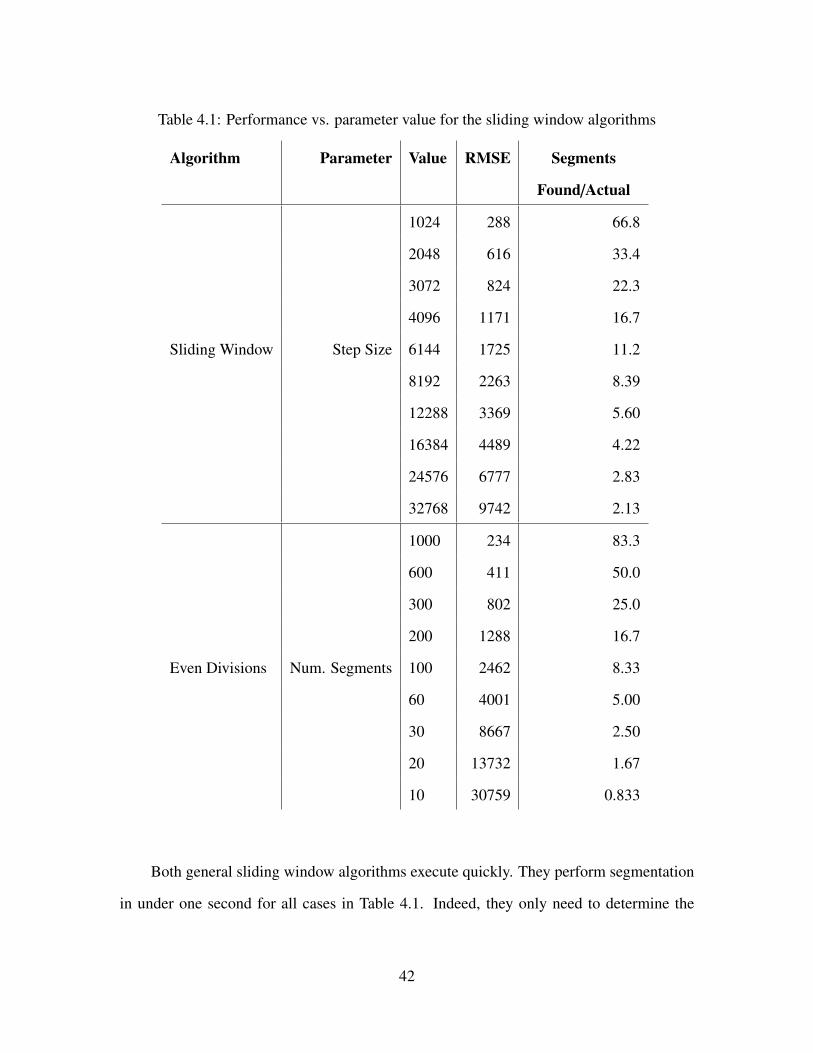
Table 4.1: Performance vs. parameter value for the sliding window algorithms

Algorithm Parameter Value RMSE Segments

Found/Actual

1024 288 66.8

2048 616 33.4

3072 824 22.3

4096 1171 16.7

Sliding Window Step Size 6144 1725 11.2

8192 2263 8.39

12288 3369 5.60

16384 4489 4.22

24576 6777 2.83

32768 9742 2.13

1000 234 83.3

600 411 50.0

300 802 25.0

200 1288 16.7

Even Divisions Num. Segments 100 2462 8.33

60 4001 5.00

30 8667 2.50

20 13732 1.67

10 30759 0.833

Both general sliding window algorithms execute quickly. They perform segmentation

in under one second for all cases in Table 4.1. Indeed, they only need to determine the

42

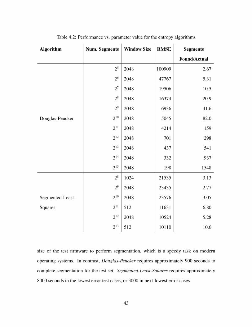
Table 4.2: Performance vs. parameter value for the entropy algorithms

Algorithm Num. Segments Window Size RMSE Segments

Found/Actual

25 2048 100909 2.67

26 2048 47767 5.31

27 2048 19506 10.5

28 2048 16374 20.9

29 2048 6936 41.6

Douglas-Peucker 210 2048 5045 82.0

211 2048 4214 159

212 2048 701 298

213 2048 437 541

214 2048 332 937

215 2048 198 1548

28 1024 21535 3.13

29 2048 23435 2.77

Segmented-Least- 210 2048 23576 3.05

Squares 211 512 11631 6.80

212 2048 10524 5.28

213 512 10110 10.6

size of the test firmware to perform segmentation, which is a speedy task on modern

operating systems. In contrast, Douglas-Peucker requires approximately 900 seconds to

complete segmentation for the test set. Segmented-Least-Squares requires approximately

8000 seconds in the lowest error test cases, or 3000 in next-lowest error cases.

43

This research selects Even Divisions as the best file segmenting algorithm of those it

tests, and uses this algorithm for the remainder of the research. The general sliding window

algorithms make the best error/segment ratio tradeoff, and run fastest. Additionally, the

Even Divisions parameter is linearly proportional to run time, and provides users with a

simple tradeoff between accuracy and computation time. Large values of the parameter (or

small input firmwares) may result in segments inappropriately small for the file type and

code classifiers, so this research enforces a minimum segment size of 512 B. This research

also uses 100 for the Num. Segments parameter, because it provides a reasonable balance

between run-time and accuracy for the available firmwares.

4.2 Classifier Analysis

Each classifier builds models to describe the training set. During testing they compare

test samples to the models to determine which model best-matches the sample. The internal

representation of the model differs by classifier, but each model must represent properties

inherent to the files it represents. The support vector machine (SVM) classifier model

is a set of weights for a neural network, and the model itself yields little insight into

the classifier performance. This section discusses the properties revealed by the classifier

models, but skips discussion of the SVM classifier. This section builds classifier models

from the training corpus. Table 4.3 describes the training corpus, which is 80% of the full

corpus as described by Table 3.1.

4.2.1 Fileprints

Fileprints represents file types as a byte-value mean frequency and variance. This

section graphs and discusses the fileprints of several file types, as generated from the

training set comprising 80% of the file corpus. Each graph represents byte values on the

X-axis and presents the mean proportion of each byte in the training files and that value’s

variance. Each graph depicts variance on a logarithmic-scale Y-axis.

44

Table 4.3: Training set characteristics

File type File Count File type File Count

GZip 352 PostScript 547

JPEG 2791 GIF 1181

PDF 1406 ARM 7140

Microsoft Word 2123 Motorola 68000 10430

Markup 10039 AVR 10799

Text 3016 PowerPC 7952

Figure 4.2 provides a reference, and is the fileprint of a set of 100 files containing

100 kB of uniformly-distributed random byte values. The expected average byte frequency

for this distribution is 1/256 = 0.39%, and Figure 4.2 shows that this expectation holds in

practice. Additionally, the random distribution has a small, flat variance profile.

GZip and Joint Photographic Experts Group (JPEG)’s fileprints are not visually

similar. Figure 4.3 shows GZip’s byte value peaks have a periodic nature, with major peaks

at bytes 127, 63, 191, and 255, and smaller peaks on every eighth byte. However, these

byte frequency peaks correspond with peaks on a variance plot that is already, generally, ten

times that of the random distribution. JPEG has no noticeable periodic nature, as Figure 4.4

depicts. It has only one major peak (besides the maximum and minimum byte values), at

byte 32. The JPEG fileprint also shows relatively large variance. Similarly, the fileprints

for Microsoft Word files and Portable Document Formats (PDFs) show relatively large

variance. Section 4.3.1 discusses the implications of this fact.

Figures 4.5 and 4.6 show that the Text and PostScript fileprints are visually similar.

Both possess similar variance distributions. However, the smallest variance values in the

Text fileprint indicate that some byte values were not present in any text files, and the

PostScript fileprint shows no such case. The largest byte frequency peak in both is at byte

45

0.38

40.

388

0.39

20.

396

Byt

e F

requ

ency

(%)

0 50 100 150 200 250

0.00

025

0.00

055

Byte Value

Var

ianc

e

Figure 4.2: Fileprint of random files

32, the American Standard Code for Information Interchange (ASCII) representation of a

space. Both fileprints show that bytes 44 through 57 and 97 through 117 occur frequently,

and these correspond to the ASCII representations of punctuation, the numbers, and most

of the lowercase alphabet.

Figure 4.7 show that Graphics Interchange Format (GIF) file byte frequency has a

periodic nature. Bytes divisible by four present more frequently, a result similar to that

of GZip files in Figure 4.3. This is because GIF images use Lempel-Ziv-Welch (LZW)

compression, an algorithm similar to GZip compression [14]. Figure 4.8 depicts the code

training files fileprint, pooling all code architectures. The code fileprint peaks correspond

with bytes present in the decision tree classifiers’ most frequently used leaves. Notably,

bytes 0x40, 0x4E, and 0x80 correspond to the peaks at 64, 78, and 128 respectively, and

Section 4.2.4 indicates that these bytes appear frequently in decision tree leaves.

46

0.4

0.8

1.2

1.6

Byt

e F

requ

ency

(%)

0 50 100 150 200 250

5e−

035e

+00

Byte Value

Var

ianc

e

Figure 4.3: Fileprint of GZip training files

0.5

1.0

1.5

2.0

Byt

e F

requ

ency

(%)

0 50 100 150 200 250

5e−

035e

+00

Byte Value

Var

ianc

e

Figure 4.4: Fileprint of JPEG training files

47

05

1015

20

Byt

e F

requ

ency

(%)

0 50 100 150 200 250

1e−

131e

−01

Byte Value

Var

ianc

e

Figure 4.5: Fileprint of Text training files

02

46

810

12

Byt

e F

requ

ency

(%)

0 50 100 150 200 250

1e−

041e

+02

Byte Value

Var

ianc

e

Figure 4.6: Fileprint of PostScript training files

48

0.5

1.0

1.5

2.0

2.5

Byt

e F

requ

ency

(%)

0 50 100 150 200 250

0.01

1.00

Byte Value

Var

ianc

e

Figure 4.7: Fileprint of GIF training files

02

46

810

14

Byt

e F

requ

ency

(%)

0 50 100 150 200 250

5e−

035e

+00

Byte Value

Var

ianc

e

Figure 4.8: Fileprint of code training files

49

4.2.2 Statistical

Figure 4.9 displays the normalized model parameters of Conti’s statistics-based

classifier, as applied to this research’s training data. Ideally, all file types have values

distinct enough to enable the classifier to distinguish between each with Euclidean distance.

Visually however, the GZip, JPEG, PDF, and GIF file types form one cluster, while the

Microsoft Word, Markup, Text, and PostScript file types form a second. This suggests that

the statistical classifier will have difficulty distinguishing between these clustered types.

oo o o

o

o

o o o

o

0.0

0.1

0.2

0.3

0.4

0.5 x

xx

x

x

x

x x

x

x

++ + +

+ ++

++

+

** * * * * * * *

*

ox+

*

Hamming WeightByte MeanEntropyChi−Square

GZip JPEG PDF GIF Word Markup Text Postscript Code Random

File Type

Nor

mal

ized

Val

ue

Figure 4.9: Statistical classifier model

Data comprising the Random file type come from a uniform distribution over all byte

values. Figure 4.9 provides the Random file type for comparison only, and shows the effect

of parameter normalization. The uniform distribution suggests that the average byte value

50

should approximate 0x80, and it does in practice. Additionally, random values should, and

do, have the highest entropy and chi-square values.

The Microsoft Word, Markup, Text, PostScript and Code file types have lower mean

byte values and entropies than the other types. Word’s hamming weight value differs

significantly from all other file types, suggesting that the classifier will have success

distinguishing its type. Unfortunately, the variance of the Word values is 10 times that

of the other file types. This indicates that these values vary more significantly between

training samples. The classifier may still have difficulty separating Word files from the rest

because it uses k-Nearest Neighbor (k-NN) with training samples. The Code file type has

a greater byte mean value than the other clustered types, suggesting that the classifier has a

method for distinguishing Code segments.

GZip, JPEG, PDF and GIF have similar values for all parameters. Their entropy

values compare to the Random file type, and show that these file types contain more

information than the others. The similarity of these types’ parameters suggest that the

classifier will confuse these types easily.

All chi-square values in Figure 4.9, except Random, are 0.02 or smaller. A non-zero

chi-square value indicates that the byte values are distributed nearly randomly. The figure’s

values indicate that all file types in the training set are significantly different from random.

This result suggests that the chi-square measure provides little information upon which the

classifier might base a decision.

4.2.3 Normalized Compression Distance

This research trains the normalized compression distance (NCD) classifier on 10% of

the training corpus due to the time constraints discussed later in Section 4.3.3. Axelsson’s

NCD classifier has little model to discuss, because it calculates little in advance. The

classifier calculates the compression length of training samples in advance, and Table 4.4

presents a summary of those values. The smallest and largest training sample compression

51

distances are 29 B and 1047 B respectively, and they belong to a code sample and a

PostScript sample respectively.

Many values in the Table 4.4 are similar, for instance, the mean compression length

of Microsoft Word and Text samples. This is not cause for concern because NCD

bases classification on a comparison of compression length of test and training samples

individually, to compression length of concatenated test and training samples. Equation 2.1

describes the comparison.

The classifier uses GZip compression, and selects multiple 1 kB disjoint sections

from training samples. When training samples are smaller than 1 kB, the classifier selects

only one section comprising the entire sample. Table 4.4 indicates that the compression

algorithm increases the length of GZip and GIF samples, and does not substantially

decrease the length of JPEG samples. This result is reasonable because compressed data

comprises the majority of files within those file types.

Table 4.4: NCD classifier training corpus model statistics

Mean Length Standard Deviation

GZip 1043.2 25.4

JPEG 1015.9 132.1

PDF 921.8 255.7

Microsoft Word 430.0 305.0

Markup 450.2 120.4

Text 437.7 126.2

PostScript 397.3 173.1

GIF 1025.6 112.9

Code 649.9 146.9

52

Table 4.4 also indicates that Microsoft Word documents have the largest standard

deviation in compression size. Word documents may contain other file formats, like GIF

and JPEG. Word documents that consist largely of those file types compress little.

The largest compression length is 1047 B, and 11% of training samples compress

to this length. The smallest compression length is 29 B, and 0.5% of training samples

compress to this length. Samples from all types compressed to these distances. These

results suggest that the classifier may have difficulty, and that future iterations of the

research should consider selecting longer training data sections.

4.2.4 Decision Tree

Figure 4.10 depicts the decision tree classifier’s model. The trained decision tree

contains only 15 leaves, indicating that it is unlikely to have over-fit the data. Its size

also suggests that information gain (IG) feature selection results in a feature set which

characterizes the training set well.

Notably, 99.8% of the AVR samples (all but 24 of 10799) contain the byte string

0xEBCD4040, and no code for other architectures contains this string. This byte string is

the most frequently used leaf in the decision tree. The string corresponds to an relative

jump followed by a subtraction from register r20. The byte string occurs as the first four

bytes, and again throughout, most of the AVR files.

The second most frequently used leaf is where byte string 0x0000004E is present,

and the tree classifies files as Motorola 68000 in that case. This decision path captures

95.9% of Motorola 68000 samples, all but 427 of 10430. Binaries in the corpus frequently

contained this byte string as the result of a jump, then a register OR with 0x00 (effectively

a no-operation instruction), then a jump.

53

Root

EBCD4040 is present: AVR

EBCD4040 is absent

4E800020 is present: PowerPC

4E800020 is absent

10402DE9 is present: ARM

10402DE9 is absent

D08DE2F0 is present: ARM

D08DE2F0 is absent

0000EBCD is present: AVR

0000EBCD is absent

A64E8004 is present: PowerPC

A64E8004 is absent

1EFF2FE1 is present: ARM

1EFF2FE1 is absent

0000A0E3 is present

FFFFFF3C is present: Motorola 68000

FFFFFF3C is absent: ARM

0000A0E3 is absent

0000004E is present: Motorola 68000

0000004E is absent

EBCD4060 is present: AVR

EBCD4060 is absent

04E02DE5 is present: ARM

04E02DE5 is absent

FFFFEB00 is present: ARM

FFFFEB00 is absent

00009421 is present: PowerPC

00009421 is absent: Motorola 68000

Figure 4.10: Decision tree classifier model

The decision tree’s third most frequently used leaf is where string 0x4E800020 is

present, classifying a sample as PowerPC. The classifier uses this leaf for 99.3% of

PowerPC samples, all but 57 of 7952. The byte string corresponds with the PowerPC blr

opcode. The opcode branches to the address in the link register, unconditionally. PowerPC

code generally places the return address for a subroutine in the link register, making blr

effectively a return statement [30].

Figure 4.10 classifies 91.1% of ARM binaries (all but 632 of 7140) with leaf

0x10402DE9, the tree’s fourth most frequently used leaf. This byte string corresponds with

54

a push, placing the contents of both register four and the link register on the stack. This

byte string frequently occurs in the function preamble, pushing those register contents, only

to pop them before returning from the function. The link register, specifically, contains the

return address for the function. ARM code frequently executes a branch to the link register

contents immediately after retrieving them with a pop.

Figures 4.11 and 4.12 depict the decision tree leaf use on the training and test sets

respectively. Each dot represents a leaf node, and dot area corresponds to the number of

samples the classifier assigns to that leaf as Table 4.5 gives. Each dot’s caption specifies

the leaf node byte string, and whether the leaf corresponds to the presence or absence of

that byte string with the letters p and a respectively. The largest dots correspond with the

leaves this section discusses. Corresponding dots in both diagrams are less than 0.2%

different, indicating that the decision tree’s performance on both sets is similar. The

research randomly assigns the test and training corpus from a larger corpus. Similar dot

size indicates that, for both test and training corpus, random assignment selects similar

proportions of files characterized by each decision tree branch.

EBCD4040(p)4E800020(p)

10402DE9(p)

D08DE2F0(p)0000EBCD(p)

A64E8004(p)

1EFF2FE1(p)FFFFFF3C(p)

FFFFFF3C(a)

0000004E(p)EBCD4060(p)

04E02DE5(p)

FFFFEB00(p)00009421(p)

00009421(a)

Figure 4.11: Decision tree leaf use on the training set

EBCD4040(p)4E800020(p)

10402DE9(p)

D08DE2F0(p)0000EBCD(p)

A64E8004(p)

1EFF2FE1(p)FFFFFF3C(p)

FFFFFF3C(a)

0000004E(p)EBCD4060(p)

04E02DE5(p)

FFFFEB00(p)00009421(p)

00009421(a)

Figure 4.12: Decision tree leaf use on the test set

55

Table 4.5: Decision tree leaf use on the test and training set

Leaf Training Test Leaf Training Test

EBCD4040 (Present) 10775 2020 FFFFFF3C (Absent) 38 5

4E800020 (Present) 7898 1477 0000004E (Present) 10005 1878

10402DE9 (Present) 6509 1220 EBCD4060 (Present) 2 0

D08DE2F0 (Present) 437 81 04E02DE5 (Present) 10 1

0000EBCD (Present) 19 5 FFFFEB00 (Present) 8 2

A64E8004 (Present) 24 5 00009421 (Present) 2 1

1EFF2FE1 (Present) 104 25 00009421 (Absent) 488 95

FFFFFF3C (Present) 2 0 Total 36321 6815

4.3 Classifier Accuracies

This section presents the results of executing each classifier independently. Table 4.6

describes the test set for the file type classifiers. The test set consists of files from the full

file corpus, which Table 3.1 describes. The test set comprises 15% of corpus files from each

file type, and the training set, described by Table 4.3, comprises another 80% of the corpus

files from each type. A cross-validation set comprises the remaining 5% of corpus files,

and is excluded from the training and testing sets. The test, training, and cross-validation

sets are mutually disjoint.

4.3.1 Fileprints

Table 4.7 depicts the Fileprints classifier producer accuracies. Highlighted cells in the

confusion matrix indicate correct matches. Fileprints’ overall accuracy, for this test set, is

71.3%. Fileprints performs better on this system’s critical file types, the Code file types.

For these types the overall accuracy is 95.6%. Accuracy on non-Code file types is 52.5%.

56

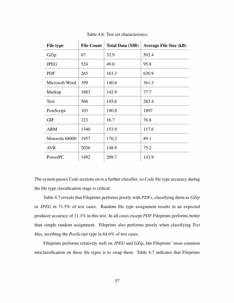
Table 4.6: Test set characteristics

File type File Count Total Data (MB) Average File Size (kB)

GZip 67 32.9 502.4

JPEG 524 49.0 95.8

PDF 265 163.3 630.9

Microsoft Word 399 140.8 361.3

Markup 1883 142.9 77.7

Text 566 145.6 263.4

PostScript 103 190.8 1897

GIF 223 16.7 76.8

ARM 1340 153.9 117.6

Motorola 68000 1957 170.2 89.1

AVR 2026 148.9 75.2

PowerPC 1492 209.7 143.9

The system passes Code sections on to a further classifier, so Code file type accuracy during

the file type classification stage is critical.

Table 4.7 reveals that Fileprints performs poorly with PDFs, classifying them as GZip

or JPEG in 71.5% of test cases. Random file type assignment results in an expected

producer accuracy of 11.1% in this test. In all cases except PDF Fileprints performs better

than simple random assignment. Fileprints also performs poorly when classifying Text

files, ascribing the PostScript type in 64.6% of test cases.

Fileprints performs relatively well on JPEG and GZip, but Fileprints’ most common

misclassification on these file types is to swap them. Table 4.7 indicates that Fileprints

57

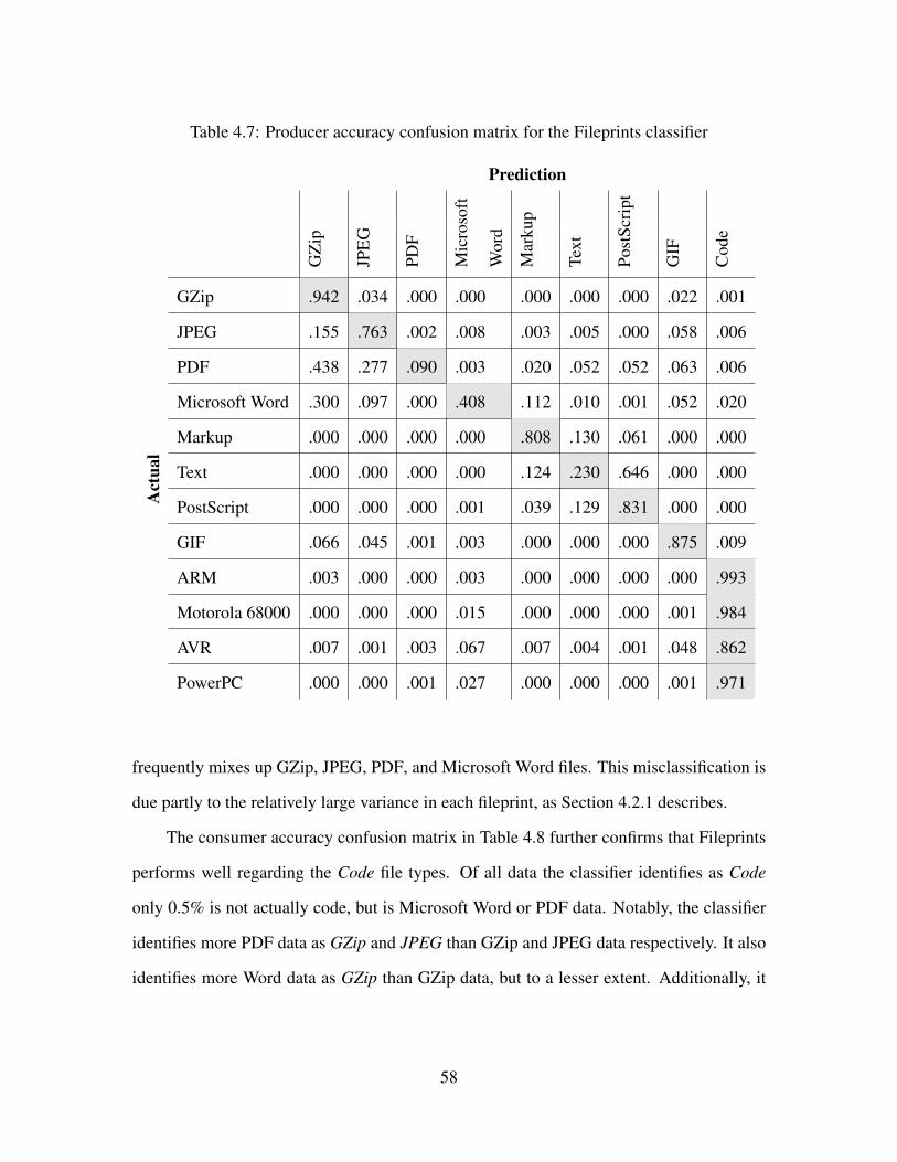
Table 4.7: Producer accuracy confusion matrix for the Fileprints classifier

Prediction

GZ

ip

JPE

G

PDF

Mic

roso

ft

Wor

d

Mar

kup

Text

Post

Scri

pt

GIF

Cod

e

Act

ual

GZip .942 .034 .000 .000 .000 .000 .000 .022 .001

JPEG .155 .763 .002 .008 .003 .005 .000 .058 .006

PDF .438 .277 .090 .003 .020 .052 .052 .063 .006

Microsoft Word .300 .097 .000 .408 .112 .010 .001 .052 .020

Markup .000 .000 .000 .000 .808 .130 .061 .000 .000

Text .000 .000 .000 .000 .124 .230 .646 .000 .000

PostScript .000 .000 .000 .001 .039 .129 .831 .000 .000

GIF .066 .045 .001 .003 .000 .000 .000 .875 .009

ARM .003 .000 .000 .003 .000 .000 .000 .000 .993

Motorola 68000 .000 .000 .000 .015 .000 .000 .000 .001 .984

AVR .007 .001 .003 .067 .007 .004 .001 .048 .862

PowerPC .000 .000 .001 .027 .000 .000 .000 .001 .971

frequently mixes up GZip, JPEG, PDF, and Microsoft Word files. This misclassification is

due partly to the relatively large variance in each fileprint, as Section 4.2.1 describes.

The consumer accuracy confusion matrix in Table 4.8 further confirms that Fileprints

performs well regarding the Code file types. Of all data the classifier identifies as Code

only 0.5% is not actually code, but is Microsoft Word or PDF data. Notably, the classifier

identifies more PDF data as GZip and JPEG than GZip and JPEG data respectively. It also

identifies more Word data as GZip than GZip data, but to a lesser extent. Additionally, it

58

identifies a relatively large amount of markup and PostScript data as Text, a large amount

of text data as PostScript, and a large amount of PDF data as GIF.

Table 4.8: Consumer accuracy confusion matrix for the Fileprints classifier

Prediction

GZ

ip

JPE

G

PDF

Mic

roso

ft

Wor

d

Mar

kup

Text

Post

Scri

pt

GIF

Cod

e

Act

ual

GZip .200 .011 .001 .000 .000 .000 .000 .017 .000

JPEG .049 .381 .006 .005 .001 .003 .000 .066 .000

PDF .461 .460 .948 .006 .020 .096 .032 .237 .001

Microsoft Word .272 .139 .003 .745 .098 .016 .001 .169 .004

Markup .000 .000 .000 .001 .716 .212 .032 .000 .000

Text .000 .000 .000 .000 .112 .384 .348 .000 .000

PostScript .000 .000 .000 .003 .046 .282 .587 .000 .000

GIF .007 .008 .001 .001 .000 .000 .000 .339 .000

ARM .003 .000 .001 .005 .000 .000 .000 .002 .233

Motorola 68000 .000 .000 .001 .033 .000 .000 .000 .004 .255

AVR .007 .001 .030 .129 .007 .006 .000 .164 .195

PowerPC .000 .000 .009 .073 .000 .000 .000 .003 .310

Table 4.9 provides an overview of Fileprints’ performance, and consists of data from

the highlighted cells of Tables 4.7 and 4.8. Table 4.9 indicates that the PDF file type’s

large consumer accuracy is due to the classifier identifying very little data as PDF. This

result is evident because PDF producer accuracy is low indicating that it identified few

PDFs correctly, yet consumer accuracy is high indicating that 94.8% of all data identified

59

as PDF is actually PDF. The Microsoft Word file type result is similar, though not to the

same extent as PDF.

Table 4.9: Fileprints classifier error summary

Producer

Accuracy

Omission

Error

Consumer

Accuracy

Commission

Error

GZip 0.942 0.058 0.200 0.800

JPEG 0.763 0.237 0.381 0.619

PDF 0.090 0.910 0.948 0.052

Microsoft Word 0.408 0.592 0.745 0.255

Markup 0.808 0.192 0.716 0.284

Text 0.230 0.770 0.384 0.616

PostScript 0.831 0.169 0.587 0.413

GIF 0.875 0.125 0.339 0.661

ARM 0.993 0.007 0.233 0.767

Motorola 68000 0.984 0.016 0.255 0.745

AVR 0.862 0.138 0.195 0.805

PowerPC 0.971 0.029 0.310 0.690

4.3.2 File Statistics

The statistical file classifier Conti et al. describe performs with an overall accuracy

of 72.7%, and accuracy among the code file types of 97.4%. The algorithm achieves a

53.6% accuracy with non-code file types. Overall, this system performs slightly better than

Fileprints, beating its accuracy by a small margin in all three cases.

Table 4.10 describes producer accuracy results for this algorithm. The classifier

performs worst with PDFs, classifying more as JPEG than PDF. Fileprints’ performance

60

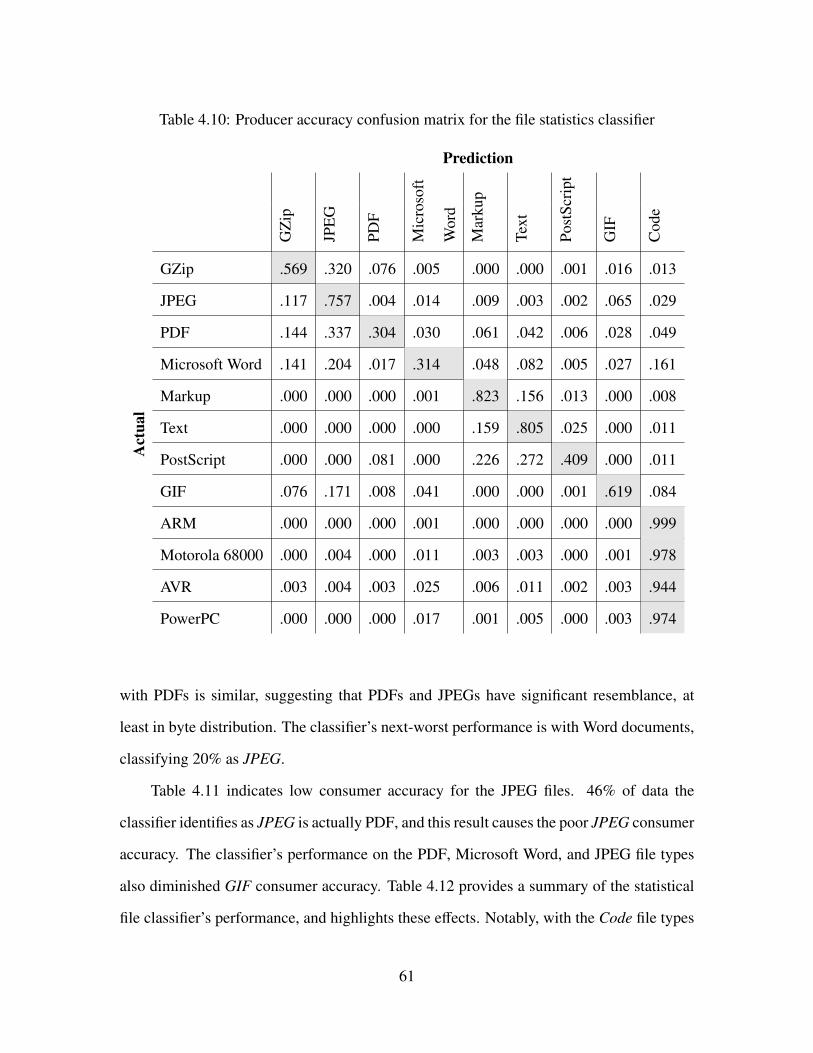
Table 4.10: Producer accuracy confusion matrix for the file statistics classifier

Prediction

GZ

ip

JPE

G

PDF

Mic

roso

ft

Wor

d

Mar

kup

Text

Post

Scri

pt

GIF

Cod

e

Act

ual

GZip .569 .320 .076 .005 .000 .000 .001 .016 .013

JPEG .117 .757 .004 .014 .009 .003 .002 .065 .029

PDF .144 .337 .304 .030 .061 .042 .006 .028 .049

Microsoft Word .141 .204 .017 .314 .048 .082 .005 .027 .161

Markup .000 .000 .000 .001 .823 .156 .013 .000 .008

Text .000 .000 .000 .000 .159 .805 .025 .000 .011

PostScript .000 .000 .081 .000 .226 .272 .409 .000 .011

GIF .076 .171 .008 .041 .000 .000 .001 .619 .084

ARM .000 .000 .000 .001 .000 .000 .000 .000 .999

Motorola 68000 .000 .004 .000 .011 .003 .003 .000 .001 .978

AVR .003 .004 .003 .025 .006 .011 .002 .003 .944

PowerPC .000 .000 .000 .017 .001 .005 .000 .003 .974

with PDFs is similar, suggesting that PDFs and JPEGs have significant resemblance, at

least in byte distribution. The classifier’s next-worst performance is with Word documents,

classifying 20% as JPEG.

Table 4.11 indicates low consumer accuracy for the JPEG files. 46% of data the

classifier identifies as JPEG is actually PDF, and this result causes the poor JPEG consumer

accuracy. The classifier’s performance on the PDF, Microsoft Word, and JPEG file types

also diminished GIF consumer accuracy. Table 4.12 provides a summary of the statistical

file classifier’s performance, and highlights these effects. Notably, with the Code file types

61

Table 4.11: Consumer accuracy confusion matrix for the file statistics classifier

Prediction

GZ

ip

JPE

G

PDF

Mic

roso

ft

Wor

d

Mar

kup

Text

Post

Scri

pt

GIF

Cod

e

Act

ual

GZip .269 .078 .035 .003 .000 .000 .000 .023 .001

JPEG .082 .274 .003 .012 .002 .001 .001 .133 .002

PDF .337 .406 .701 .081 .049 .032 .011 .189 .011

Microsoft Word .286 .212 .033 .738 .033 .054 .008 .159 .032

Markup .000 .000 .001 .001 .581 .104 .021 .000 .002

Text .000 .000 .000 .000 .114 .549 .042 .000 .002

PostScript .000 .000 .218 .000 .213 .243 .913 .000 .003

GIF .018 .021 .002 .012 .000 .000 .000 .435 .002

ARM .000 .000 .000 .002 .000 .000 .000 .001 .218

Motorola 68000 .000 .004 .001 .030 .002 .003 .001 .010 .237

AVR .007 .004 .006 .061 .004 .008 .003 .021 .200

PowerPC .000 .000 .000 .060 .001 .005 .000 .029 .290

5.5% of data the statistical classifier identifies as Code is not. This value is ten times that

of Fileprints. This difference in consumer accuracy makes the analyst’s job more difficult

when using the statistical classifier.

4.3.3 Normalized Compression Distance

Table 4.13 presents the NCD classifier producer accuracy. For the 9-class classification

problem random guessing produces producer accuracies of 11.1%. In all cases, the NCD

classifier performs worse than random guessing. This may reflect problems with the

62

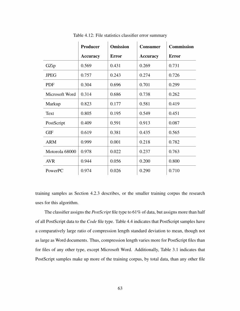
Table 4.12: File statistics classifier error summary

Producer

Accuracy

Omission

Error

Consumer

Accuracy

Commission

Error

GZip 0.569 0.431 0.269 0.731

JPEG 0.757 0.243 0.274 0.726

PDF 0.304 0.696 0.701 0.299

Microsoft Word 0.314 0.686 0.738 0.262

Markup 0.823 0.177 0.581 0.419

Text 0.805 0.195 0.549 0.451

PostScript 0.409 0.591 0.913 0.087

GIF 0.619 0.381 0.435 0.565

ARM 0.999 0.001 0.218 0.782

Motorola 68000 0.978 0.022 0.237 0.763

AVR 0.944 0.056 0.200 0.800

PowerPC 0.974 0.026 0.290 0.710

training samples as Section 4.2.3 describes, or the smaller training corpus the research

uses for this algorithm.

The classifier assigns the PostScript file type to 61% of data, but assigns more than half

of all PostScript data to the Code file type. Table 4.4 indicates that PostScript samples have

a comparatively large ratio of compression length standard deviation to mean, though not

as large as Word documents. Thus, compression length varies more for PostScript files than

for files of any other type, except Microsoft Word. Additionally, Table 3.1 indicates that

PostScript samples make up more of the training corpus, by total data, than any other file

63

Table 4.13: Producer accuracy confusion matrix for the NCD classifier

Prediction

GZ

ip

JPE

G

PDF

Mic

roso

ft

Wor

d

Mar

kup

Text

Post

Scri

pt

GIF

Cod

e

Act

ual

GZip .000 .000 .000 .000 .000 .013 .986 .000 .000

JPEG .000 .004 .002 .000 .000 .149 .842 .000 .002

PDF .000 .015 .002 .029 .001 .018 .864 .003 .068

Microsoft Word .000 .023 .031 .016 .100 .095 .561 .041 .132

Markup .000 .002 .000 .166 .000 .002 .031 .003 .796

Text .000 .024 .000 .396 .000 .000 .002 .211 .366

PostScript .000 .077 .003 .273 .000 .000 .000 .107 .539

GIF .000 .001 .000 .001 .001 .129 .867 .000 .000

ARM .000 .000 .018 .000 .013 .022 .947 .000 .000

Motorola 68000 .000 .000 .000 .000 .014 .032 .953 .000 .000

AVR .000 .001 .005 .005 .012 .047 .908 .004 .019

PowerPC .000 .000 .000 .000 .020 .050 .929 .000 .000

type except code. The large proportion of training samples and wide range of compression

lengths may make it too difficult for the NCD classifier to succeed.

Table 4.14 provides the consumer accuracy, and shows that the classifier assigns Word

documents to every type except Word. Table 4.15 provides the error summary results, and

shows the classifier is less than 5% accurate, in all cases, on this test set.

The NCD classifier requires 7.6 days to classify the test corpus, while Fileprints and

the statistical classifier require 3.5 days each. The NCD classifier can perform only one

out of three compressions during the training phase, the other two require the test sample.

64

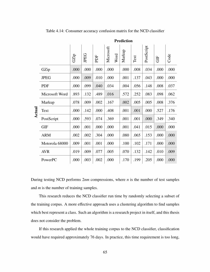
Table 4.14: Consumer accuracy confusion matrix for the NCD classifier

Prediction

GZ

ip

JPE

G

PDF

Mic

roso

ft

Wor

d

Mar

kup

Text

Post

Scri

pt

GIF

Cod

e

Act

ual

GZip .000 .000 .000 .000 .000 .008 .034 .000 .000

JPEG .000 .009 .010 .000 .001 .137 .043 .000 .000

PDF .000 .099 .040 .034 .004 .056 .148 .008 .037

Microsoft Word .893 .132 .489 .016 .572 .252 .083 .098 .062

Markup .078 .009 .002 .167 .002 .005 .005 .008 .376

Text .000 .142 .000 .408 .001 .001 .000 .527 .176

PostScript .000 .593 .074 .369 .001 .001 .000 .349 .340

GIF .000 .001 .000 .000 .001 .041 .015 .000 .000

ARM .002 .002 .304 .000 .080 .065 .153 .000 .000

Motorola 68000 .009 .001 .001 .000 .100 .102 .171 .000 .000

AVR .019 .009 .077 .005 .070 .132 .142 .010 .009

PowerPC .000 .003 .002 .000 .170 .199 .205 .000 .000

During testing NCD performs 2nm compressions, where n is the number of test samples

and m is the number of training samples.

This research reduces the NCD classifier run time by randomly selecting a subset of

the training corpus. A more effective approach uses a clustering algorithm to find samples

which best represent a class. Such an algorithm is a research project in itself, and this thesis

does not consider the problem.

If this research applied the whole training corpus to the NCD classifier, classification

would have required approximately 76 days. In practice, this time requirement is too long,

65

Table 4.15: NCD classifier error summary

Producer

Accuracy

Omission

Error

Consumer

Accuracy

Commission

Error

GZip 0.000 1.000 0.000 1.000

JPEG 0.004 0.996 0.009 0.991

PDF 0.002 0.998 0.040 0.960

Microsoft Word 0.016 0.984 0.016 0.984

Markup 0.000 1.000 0.002 0.998

Text 0.000 1.000 0.001 0.999

PostScript 0.000 1.000 0.000 1.000

GIF 0.000 1.000 0.000 1.000

ARM 0.000 1.000 0.000 1.000

Motorola 68000 0.000 1.000 0.000 1.000

AVR 0.019 0.981 0.009 0.991

PowerPC 0.000 1.000 0.000 1.000

and it hinders firmware analysis. The Fileprints and statistical classifiers permit model

calculation in advance, so training time does not impact firmware analysis. After training

they require comparatively little time to classify a sample.

4.3.4 Code Classifiers

The decision tree and SVM classifiers perform well overall, with overall accuracies

greater than 99%. Their overall errors were 5.12 × 10−3 and 1.85 × 10−5 respectively.

Table 4.16 displays the code classifier errors in detail. The code classifier accuracies are so

high that error provides a more accurate picture. In several instances the code classifiers

are 100% accurate.

66

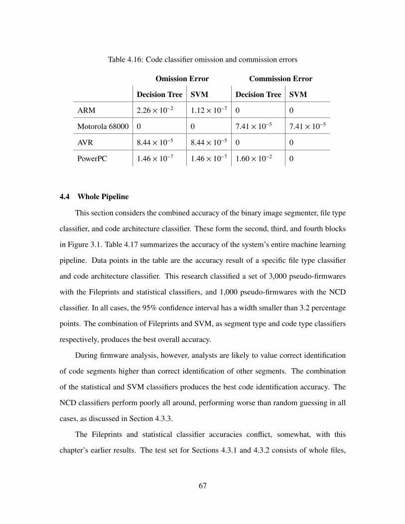
Table 4.16: Code classifier omission and commission errors

Omission Error Commission Error

Decision Tree SVM Decision Tree SVM

ARM 2.26 × 10−2 1.12 × 10−7 0 0

Motorola 68000 0 0 7.41 × 10−5 7.41 × 10−5

AVR 8.44 × 10−5 8.44 × 10−5 0 0

PowerPC 1.46 × 10−7 1.46 × 10−7 1.60 × 10−2 0

4.4 Whole Pipeline

This section considers the combined accuracy of the binary image segmenter, file type

classifier, and code architecture classifier. These form the second, third, and fourth blocks

in Figure 3.1. Table 4.17 summarizes the accuracy of the system’s entire machine learning

pipeline. Data points in the table are the accuracy result of a specific file type classifier

and code architecture classifier. This research classified a set of 3,000 pseudo-firmwares

with the Fileprints and statistical classifiers, and 1,000 pseudo-firmwares with the NCD

classifier. In all cases, the 95% confidence interval has a width smaller than 3.2 percentage

points. The combination of Fileprints and SVM, as segment type and code type classifiers

respectively, produces the best overall accuracy.

During firmware analysis, however, analysts are likely to value correct identification

of code segments higher than correct identification of other segments. The combination

of the statistical and SVM classifiers produces the best code identification accuracy. The

NCD classifiers perform poorly all around, performing worse than random guessing in all

cases, as discussed in Section 4.3.3.

The Fileprints and statistical classifier accuracies conflict, somewhat, with this

chapter’s earlier results. The test set for Sections 4.3.1 and 4.3.2 consists of whole files,

67

Table 4.17: Overall accuracy summary, and 95% confidence interval

Fileprints Statistical NCD

Decision Decision Decision

File Type Tree SVM Tree SVM Tree SVM

Non-Code .577 ± .016 .577 ± .016 .323 ± .013 .323 ± .013 .004 ± .001 .004 ± .001

Code .817 ± .012 .827 ± .012 .846 ± .011 .858 ± .010 .039 ± .005 .040 ± .005

Overall .607 ± .014 .609 ± .014 .381 ± .013 .383 ± .013 .005 ± .001 .005 ± .001

while this section uses a pseudo-firmware test set. Section 3.4 describes the construction

of pseudo-firmwares, which approximate true firmwares. The test set difference causes this

section’s accuracy values to differ from those in earlier sections.

The consumer accuracy of the code segment classifications is also likely to concern

analysts. One might focus analysis only on firmware sections classified as code segments,

and in that case a higher consumer accuracy gives the analyst less data to sift through. For

the Fileprints/SVM combination, the consumer accuracy of the code file types pooled is

86.7%. For the statistical/SVM combination the same consumer accuracy value is 66.2%.

The values are significantly different because the statistical classifier incorrectly identifies

4.2% of non-code data as code, while the Fileprints classifier only did so for 0.8%.

This research uses the Fileprints/SVM combination for firmware reverse engineering

because of the superior code segment consumer accuracy and overall producer accuracy.

The statistical/SVM classifier combination realizes a better code segment producer

accuracy, but the difference is small compared to the advantage of Fileprints/acSVM.

Table 4.18 details the system producer accuracies. In all cases, the 95% confidence

interval is smaller than 5.4 percentage points. For non-code file types, results are the same

regardless of code classifier because the code classifier does not consider segments that the

68

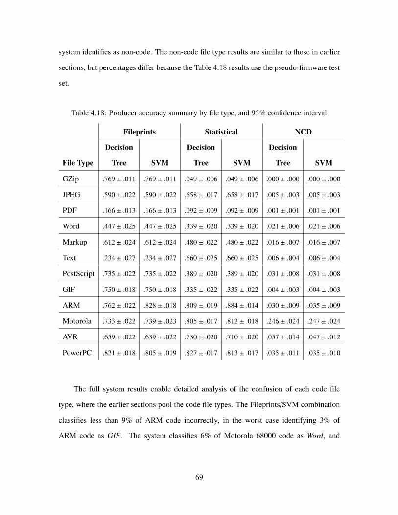
system identifies as non-code. The non-code file type results are similar to those in earlier

sections, but percentages differ because the Table 4.18 results use the pseudo-firmware test

set.

Table 4.18: Producer accuracy summary by file type, and 95% confidence interval

Fileprints Statistical NCD

Decision Decision Decision

File Type Tree SVM Tree SVM Tree SVM

GZip .769 ± .011 .769 ± .011 .049 ± .006 .049 ± .006 .000 ± .000 .000 ± .000

JPEG .590 ± .022 .590 ± .022 .658 ± .017 .658 ± .017 .005 ± .003 .005 ± .003

PDF .166 ± .013 .166 ± .013 .092 ± .009 .092 ± .009 .001 ± .001 .001 ± .001

Word .447 ± .025 .447 ± .025 .339 ± .020 .339 ± .020 .021 ± .006 .021 ± .006

Markup .612 ± .024 .612 ± .024 .480 ± .022 .480 ± .022 .016 ± .007 .016 ± .007

Text .234 ± .027 .234 ± .027 .660 ± .025 .660 ± .025 .006 ± .004 .006 ± .004

PostScript .735 ± .022 .735 ± .022 .389 ± .020 .389 ± .020 .031 ± .008 .031 ± .008

GIF .750 ± .018 .750 ± .018 .335 ± .022 .335 ± .022 .004 ± .003 .004 ± .003

ARM .762 ± .022 .828 ± .018 .809 ± .019 .884 ± .014 .030 ± .009 .035 ± .009

Motorola .733 ± .022 .739 ± .023 .805 ± .017 .812 ± .018 .246 ± .024 .247 ± .024

AVR .659 ± .022 .639 ± .022 .730 ± .020 .710 ± .020 .057 ± .014 .047 ± .012

PowerPC .821 ± .018 .805 ± .019 .827 ± .017 .813 ± .017 .035 ± .011 .035 ± .010

The full system results enable detailed analysis of the confusion of each code file

type, where the earlier sections pool the code file types. The Fileprints/SVM combination

classifies less than 9% of ARM code incorrectly, in the worst case identifying 3% of

ARM code as GIF. The system classifies 6% of Motorola 68000 code as Word, and

69

3% of PowerPC code as GIF. For all three architectures the system has no other type

misclassifications greater than 2%.

Of the code file types, the Fileprints/SVM combination shows the worst performance

with AVR. It classifies 11% of AVR code as Motorola, and 2% total as ARM or PowerPC.

Thus, the system classifies 80% of AVR code as Code, though it gets the architecture wrong

nearly 1 time out of 6. In practice, this observation suggests that the system would identify

the majority of code and apply the correct architecture, giving an analyst a strong hint as to

the correct architecture. The system labels 9% of AVR code as GIF, 5% as Word document,

and a further 3% as PDF or GZip.

Considering consumer accuracies, 20% of data the system identifies as Motorola

68000 code is actually Word document. As Table 4.6 shows, the average Word document

size is four times that of Motorola files, and the random firmware generator includes

amounts of data proportional to file size. Consequently, the number of Word document

bytes in the pseudo-firmwares is approximately four times that of Motorola 68000 bytes.

Some analysis reveals that this proportion of documentation to code is uncharacteristic

of real firmwares, and in this case the pseudo-firmwares do not adequately model real

firmwares. The 20% value is a consequence of the poor accuracy of Fileprints on Word

documents, and the disproportionate amount of Word document bytes to Motorola 68000

bytes.

4.5 Opcode Analysis

After finding a likely match for a code section’s architecture, the system disassembles

that section. Disassembly must start at the correct byte offset, and in the firmware image

byte offsets are arbitrary. The system does not automatically detect code offsets, instead

disassembling code sections at all likely offsets for the identified architecture. For each of

the architectures this research considers, the system tries offsets of zero, one, two, and three

bytes.

70

In practice, each disassembly produces a different set of partially-valid code, and the

correct disassembly is not obvious. The analyst must manually consider each disassembly

and determine which is correct. Appendix A illustrates the difficulty of determining the

correct disassembly by providing four disassemblies of a small code section.

Opcode frequency analysis is one method for assisting in the process. The system

automates this process by determining the frequency of all opcodes in each disassembly. It

then orders the opcodes by frequency, and compares the list to one from other binaries of

that architecture. It annotates the ordered list by marking those opcodes that comprise 90%

of other binaries. Those opcodes generally appear more frequently in correct disassemblies

than in incorrect disassemblies. Appendix A provides a portion of the opcode analysis

from a real firmware, and illustrates how an analyst uses that data to determine the correct

disassembly.

Table 4.19 presents the results of analyzing 100 Executable and Linkable Format

(ELF) binaries from each of this research’s four architectures. Each ELF comes from the

test and training corpus described in Section 3.4. Appendix B presents the most frequent

100 opcodes from each architecture, along with frequency values.

Table 4.19: Most frequent opcodes from four architectures

ARM PowerPC

Opcode Description Opcode Description

ldr Load word lwz Load word and zero

mov Move mr Move register

add Add stw Store word

bl Branch and link bl Branch and link

str Store addi Add

cmp Compare li Load

71

b Unconditional branch b Branch

beq Conditional branch cmpwi Compare

bx Branch and exchange beq Conditional branch

andeq Conditional and mtctr Move

sub Subtract bne Conditional branch

bne Conditional branch nop No operation

ldrb Load mflr Move

push Push bctrl Unconditional branch

pop Pop blr Unconditional branch

lsl Shift left mtlr Move

ldm Load multiple bctr Unconditional branch

strb Store byte stwu Store word

movne Conditional move lis Add

subs Subtract rlwinm Rotate word left then And

add Add

cmpw Compare

stfd Store

addis Add

Motorola 68000 AVR

Opcode Description Opcode Description

movel Move sbc Subtract with carry

moveal Move-aligned sbci Subtract with carry

bsrl Branch to subroutine rjmp Relative jump

addql Add quick ori Or

72

lea Load effective address cpi Compare

clrl Clear ldd Load indirect

pea Push effective address cp Compare

tstl Test operand ldi Load

moveq Move quick sub Subtract

beqs Conditional branch rcall Call subroutine

unlk Unlink subi Subtract

cmpl Compare andi And

rts Return from subroutine add Add

moveml Move multiple or Or

beqw Conditional branch mul Multiply unsigned

braw branch std Store indirect

jsr Jump to subroutine cpc Compare with carry

bral Branch in Input from I/O

addl Add adc Add with carry

jmp Jump out Output to I/O

bnes Conditional branch mov Move

moveb Move nop No operation

lsll Left shift eor Exclusive or

bras Branch ld Load

linkw Link sbis Conditional skip

bnew Conditional branch cbi Clear bits

subql Subtract quick muls Multiply signed

fmoved Move

73

Table 4.19 provides a description for the most frequent opcodes that comprise

90% of each architecture’s opcodes. These opcodes fall into four categories based on

how the compiler generally employs them. Figure 4.13 depicts the proportions each

category comprises for each architecture. Notably, for each architecture approximately

25% of instructions are control instructions like branch or jump. For the Motorola

68000 architecture, over 40% of instructions were move-like instructions (movel, moveal,

moveq...).

ARM Motorola 68000 PowerPC AVR

Fre

quen

cy

0.0

0.2

0.4

0.6

0.8

ControlArithmeticMemoryNo Operation

Architecture

Fre

quen

cy

Figure 4.13: Proportions of opcode type

4.6 Firmware Disassembly

While the classifier’s performance on test sets is encouraging, the true goal of

the system is to disassemble real-world firmwares. This section presents the results

of disassembling several Allen-Bradley firmwares. The results from disassembling real

74

firmwares validate this research’s results from pseudo-firmwares. Allen-Bradley includes

each within a firmware update tool containing approximately 190 firmware-like binary

images. Three categories describe the firmware contents, as Table 4.20 shows. This section

details the contents of one firmware from categories one and two, specifically the bold

firmwares in Table 4.20.

Table 4.20: Categorization of firmware contents

Category Firmwares

PPC & ZLib 99449204, 99472767, PN-20032, 99472769,

99469405

ARM & ZLib PN-20028, PN-19989, 99502404, 99482558

PN-20008, PN-50978, PN-20017, PN-50984

ARM Only 99502504, PN-19990

4.6.1 PPC & ZLib - Firmware 99449204.bin

Firmwares in the PPC & ZLib category consist of a binary image with short data and

code segments followed by a large, nearly 800 kB, ZLib-compressed segment. The ZLib

segment consists of code for PowerPC architecture central processing units (CPUs). With

the exception of 99469405.wbn, PPC & ZLib firmwares also contain a File Allocation

Table (FAT) file system. Firmware 99469405.wbn is 960 kB, while the other PPC & ZLib

firmwares are between 1.6 MB and 1.8 MB. Peck and Peterson document their disassembly

of the PPC & ZLib firmware 99472767.wbn [48].

The directory that contains firmware image 99449204.bin contains two other files.

One contains only four bytes, and provides no immediate insights into the firmware

contents. The other, 99449204.nvs, is a configuration file for the firmware update tool.

It contains a line that reveals the destination hardware’s identity as 1788-ENBT. The

75

1788-ENBT is an Ethernet daughtercard for FlexLogix Programmable Logic Controllers

(PLCs) providing Internet Protocol (IP) over Ethernet.

With its default settings, Foremost extracts 78 files from the firmware binary.

Table 4.21 summarizes Foremost’s results. Of the 33 bitmap files Foremost reveals, nine

are valid bitmaps and the remainder only contained part of the bitmap header. Foremost

extracts 19 valid GIF images. All valid bitmap and GIF images are small icons, likely for

use within a webpage. Microsoft Windows executables that Foremost produces are only

portions of the binary file that contain the common MZ magic number, but are not actually

Windows executables.

Foremost extracts 15 HyperText Markup Language (HTML) documents. Each

references several GIF images with names matching the contents of the GIF files Foremost

produces. These documents form a website displaying status information for the Ethernet

interface. The website displays Simple Mail Transfer Protocol (SMTP), Domain Name

System (DNS), and basic network configuration properties. It references Javascript files

containing a simple client-side Javascript API to retrieve settings dynamically. Foremost

output does not include the Javascript files.

Table 4.21: Summary of Foremost output for the firmware

File Type Produced Valid

Bitmap 33 9

GIF 19 19

HTML 15 15

Windows Executable 11 0

Listing the strings within the firmware reveals copyright messages from 2004,

error, and status messages, but also the strings “Dhrystone Benchmark, Version 2.1”

76

and “VxWorks 5.5, Mar 31 2005, 11:29:31”. These strings suggest that the firmware

incorporates the popular Dhrystone CPU benchmark [75], and that some component of

the firmware comes from the VxWorks 5.5 embedded operating system [76].

The Firmware Disassembly System identifies and outputs one ZLib-compressed

section and 16 non-compressed sections within the firmware. Table 4.22 summarizes

the system’s results, and compares them to a manual inspection of the firmware’s results.

The system completed firmware analysis in 100 seconds on a consumer-grade laptop with

4 GB random-access memory (RAM) and a dual-core 2.3 GHz CPU. The large PowerPC

and Motorola sections, within the system’s results, indicate byte-ranges that merit further

analysis.

Bytes 0 through 56904 contain three general sections. The first is a header with ASCII

text copyright statements, but otherwise unknown content. The largest section contains

binary data which disassembles into plausible assembly code for the PowerPC architecture.

Bytes 96774 through 113907 likewise disassemble into plausible PowerPC assembly code

when the disassembler uses an offset of two bytes.

The firmware code sections lack any clear metadata, and this makes choosing

the correct section disassembly difficult. Disassembly requires correct specification of

architecture and code byte offset. Both requirements are difficult to identify because

most byte values resolve to an opcode in the four architectures this research considers.

Comparing opcode frequency with the training set gives some clue as to whether a

particular disassembly is correct. Also, correct code disassembly generally produces a

large number of cross-references within the code. These two techniques provide an analyst

some insight into a disassembly’s correctness.

The Firmware Disassembly System correctly identifies a ZLib-compressed section

consisting of bytes 113907 through 889823. It automatically uncompresses this section and

performs analysis on it recursively. Uncompressed, the section requires 1.9 MB, but much

77

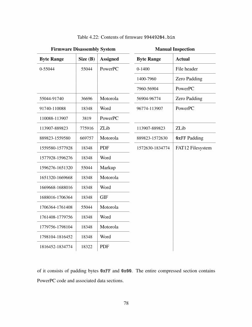
Table 4.22: Contents of firmware 99449204.bin

Firmware Disassembly System Manual Inspection

Byte Range Size (B) Assigned Byte Range Actual

0-55044 55044 PowerPC 0-1400 File header

1400-7960 Zero Padding

7960-56904 PowerPC

55044-91740 36696 Motorola 56904-96774 Zero Padding

91740-110088 18348 Word 96774-113907 PowerPC

110088-113907 3819 PowerPC

113907-889823 775916 ZLib 113907-889823 ZLib

889823-1559580 669757 Motorola 889823-1572630 0xFF Padding

1559580-1577928 18348 PDF 1572630-1834774 FAT12 Filesystem

1577928-1596276 18348 Word

1596276-1651320 55044 Markup

1651320-1669668 18348 Motorola

1669668-1688016 18348 Word

1688016-1706364 18348 GIF

1706364-1761408 55044 Motorola

1761408-1779756 18348 Word

1779756-1798104 18348 Motorola

1798104-1816452 18348 Word

1816452-1834774 18322 PDF

of it consists of padding bytes 0xFF and 0x00. The entire compressed section contains

PowerPC code and associated data sections.

78

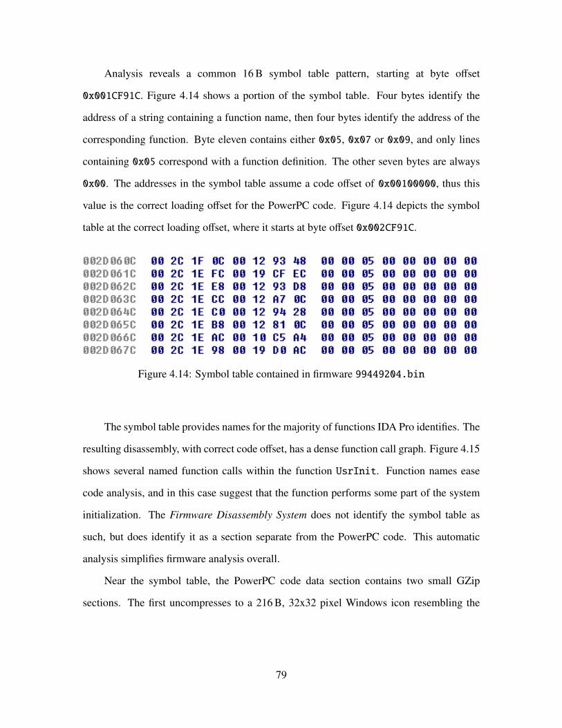
Analysis reveals a common 16 B symbol table pattern, starting at byte offset

0x001CF91C. Figure 4.14 shows a portion of the symbol table. Four bytes identify the

address of a string containing a function name, then four bytes identify the address of the

corresponding function. Byte eleven contains either 0x05, 0x07 or 0x09, and only lines

containing 0x05 correspond with a function definition. The other seven bytes are always

0x00. The addresses in the symbol table assume a code offset of 0x00100000, thus this

value is the correct loading offset for the PowerPC code. Figure 4.14 depicts the symbol

table at the correct loading offset, where it starts at byte offset 0x002CF91C.

Figure 4.14: Symbol table contained in firmware 99449204.bin

The symbol table provides names for the majority of functions IDA Pro identifies. The

resulting disassembly, with correct code offset, has a dense function call graph. Figure 4.15

shows several named function calls within the function UsrInit. Function names ease

code analysis, and in this case suggest that the function performs some part of the system

initialization. The Firmware Disassembly System does not identify the symbol table as

such, but does identify it as a section separate from the PowerPC code. This automatic

analysis simplifies firmware analysis overall.

Near the symbol table, the PowerPC code data section contains two small GZip

sections. The first uncompresses to a 216 B, 32x32 pixel Windows icon resembling the

79

Figure 4.15: Code from the function UsrInit

1788-ENBT Ethernet card. The second is an Allen-Bradley electronic data sheet (EDS)

network configuration file, providing basic information about the Ethernet card.

4.6.2 ARM & ZLib - Firmware PN-20028.bin

ARM & ZLib firmwares begin with an ARM code segment, then contain between two

and fourteen compressed files, then end with multiple short data segments separated by

0x00 or 0xFF padding bytes. Each firmware is between 1.4 MB and 1.9 MB in size, and

the ARM segment comprises between 1.2 and 1.8 MB.

At least two configuration files, with the .nvs file extension, refer to firmware

PN-20028.bin. They indicate that it targets both the 1769-L32E and 1769-L32C devices.

Both devices are communications modules for CompactLogix PLCs [54]. The .nvs files

indicate that firmwares PN-20032.bin and PN-20030.bin target devices 1769-L32E and

1769-L32C respectively. Firmware PN-20032 is a PPC& ZLib firmware, and this research

does not investigate firmware PN-20030.

Foremost produces one JPEG and one bitmap (BMP) file. The JPEG file contains the

magic number 0xFFD8FF, while the BMP file contains the magic number BM. Neither file

is a valid image, they contain sections of binary data that include JPEG and BMP magic

80

numbers. Listing the strings within the firmware produces device names, error messages,

source file names, and the compiler name. The device names are consistent with this

section’s analysis. Strings reveal that the code is C or C++, and the compiler toolkit is

the ARM Developer Suite version 1.2, released in November 2001 [6].

Table 4.23 describes the Firmware Disassembly System output and the results of

manual firmware inspection. The firmware’s strings suggest that it contains code for ARM

architecture processors, and the Firmware Disassembly System output indicates that ARM

code comprises the majority of the firmware. The ARM code sections merit further analyst

attention. Additionally, the system suggests that a zero byte offset results in correct code

disassembly.

Table 4.23: Contents of firmware PN-20028.bin

Firmware Disassembly System Manual Inspection

Byte Range Size (B) Assigned Byte Range Actual

0-1538024 1538024 ARM 0-1744908 ARM

1538024-1541673 3649 Word

1541673-1555908 14235 PowerPC

1555908-1573792 17884 GIF

1573792-1627444 53652 Motorola

1627444-1663212 35768 ARM

1663212-1744908 81696 Word

1744908-1756829 11921 16 ZLib Files 1744908-1756829 16 ZLib Files

1756829-1781248 24419 Word 1756829-1788344 Sparse binary data,

unknown format

1781248-1785924 4676 Motorola

1785924-1788344 2420 ARM

81

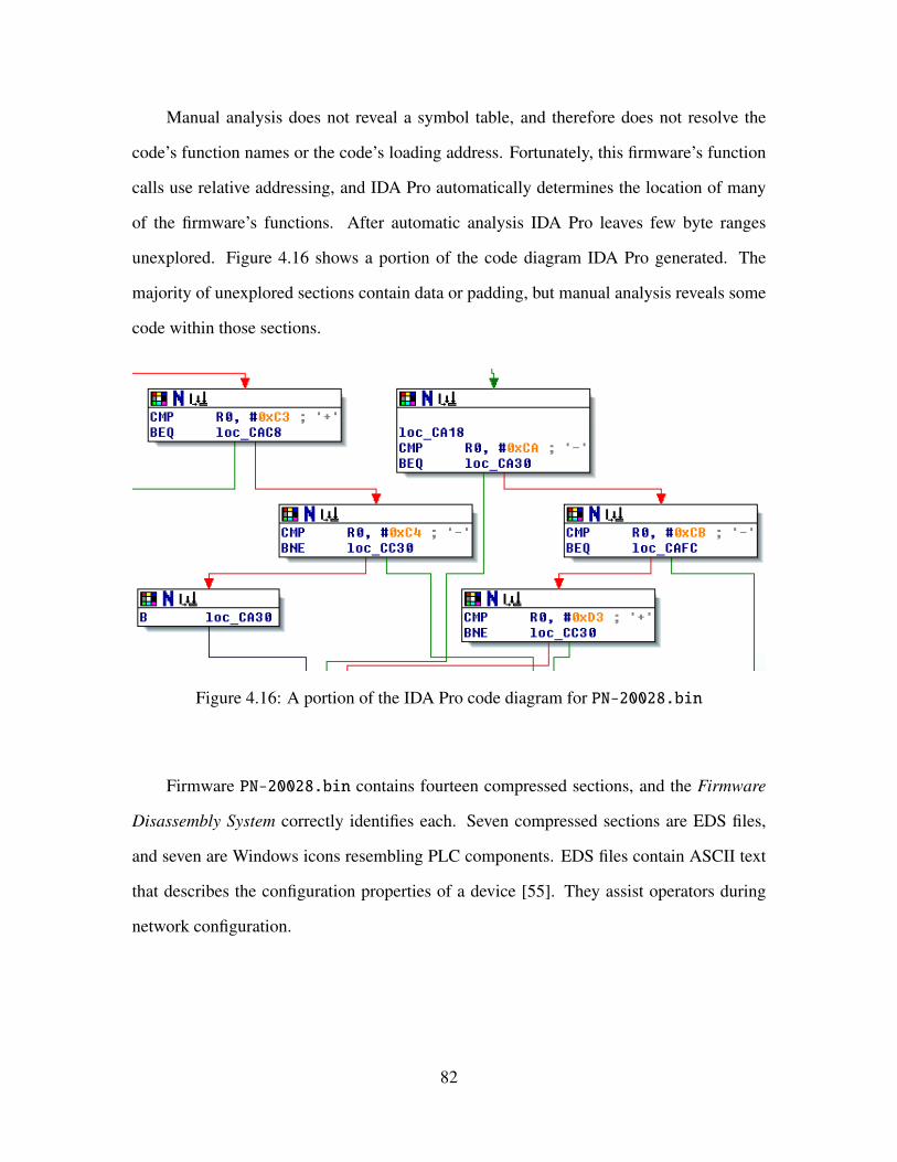
Manual analysis does not reveal a symbol table, and therefore does not resolve the

code’s function names or the code’s loading address. Fortunately, this firmware’s function

calls use relative addressing, and IDA Pro automatically determines the location of many

of the firmware’s functions. After automatic analysis IDA Pro leaves few byte ranges

unexplored. Figure 4.16 shows a portion of the code diagram IDA Pro generated. The

majority of unexplored sections contain data or padding, but manual analysis reveals some

code within those sections.

Figure 4.16: A portion of the IDA Pro code diagram for PN-20028.bin

Firmware PN-20028.bin contains fourteen compressed sections, and the Firmware

Disassembly System correctly identifies each. Seven compressed sections are EDS files,

and seven are Windows icons resembling PLC components. EDS files contain ASCII text

that describes the configuration properties of a device [55]. They assist operators during

network configuration.

82

4.6.3 ARM Only

The ARM Only firmwares are similar to the ARM & ZLib firmwares, but only

contain an ARM code section. Additionally, ARM Only firmwares are smaller. Both are

approximately 170 kB. IDA Pro’s automatic analysis identifies many function entry points,

as it did for ARM & ZLib firmwares.

4.6.4 Strengths and Weaknesses

This exercise reveals some strengths and weaknesses of the current iteration of the

Firmware Disassembly System. The system significantly reduces the time required for

firmware analysis by automatically identifying relevant sections. It automatically identifies

the architecture of code sections and disassembles them. The system automatically finds

compressed sections within the firmware and recursively analyzes them.

Unfortunately, the Firmware Disassembly System performs poorly when it encounters

sections filled with padding. Padding bytes 0x00 and 0xFF cause the system to identify

sections as Motorola 68000 code. Figures 4.17 and 4.18 summarize the system’s

performance on firmwares 99449204.bin and PN-20028.bin, respectively. The system

misidentifies each padding byte range, in Figure 4.17, as Motorola 68000. This

misclassification only slightly hinders analysis efforts, as the system’s error is evident

upon brief inspection. Figure 4.18 contains no padding byte ranges because firmware

PN-20028.bin only contains small padding segments. The file segmenter includes those

small padding segments within larger segments, which the system then misclassifies as

Word as Table 4.23 shows. Future iterations of the Firmware Disassembly System may

address the padding section misclassification by finding large sections of padding bytes

and removing them prior to further analysis.

83

0 .5 1 1.5 2Byte Offset (MB)

CorrectIncorrectPadding

Figure 4.17: Summary of system performance on firmware 99449204.bin

0 .5 1 1.5 2Byte Offset (MB)

CorrectIncorrectPadding

Figure 4.18: Summary of system performance on firmware PN-20028.bin

84

5 Conclusions

This research described the algorithms comprising the Firmware Disassembly System,

a tool to assist analysts with PLC firmware disassembly. The system found compressed

sections, determined the file type of byte ranges within the firmware, automatically

disassembled likely code sections, and provided opcode frequency analysis for human

reference. The process required machine learning algorithms, and the majority of this

research involved selecting those algorithms.

The machine learning algorithms that identified firmware segment file types required

firmware segments upon which to operate. Section 4.1 analyzed the performance of four

file segmenting algorithms. Two were variations on a sliding window, and two used a

measure of instantaneous file entropy. The sliding window algorithms outperformed the

entropy algorithms, both in speed and accuracy. Consequently, the Firmware Disassembly

System segmented files with a sliding window. Specifically, it divided files into 100

segments, or 512 B segments, whichever are larger.

Identifying the file type of byte ranges is similar to a technique called file carving, so

this research applied three file carving algorithms to the problem. One algorithm considered

four statistical features of each sample, while another used normalized compression

distance. This research revealed that the most successful file carving algorithm for this

problem was Fileprints. Fileprints models file types as the mean and variance of byte-value

frequency in the training set. On a 10,845 file test corpus consisting of 9 classes of file

type, Fileprints achieved a 71.3% accuracy overall, and a 95.6% accuracy when identifying

executable code segments.

After the file type classifier identifies the file type of each segment, another machine

learning algorithm must identify the architecture and endianness of the code segments. This

research applied two malware identification algorithms to the code classification problem.

85

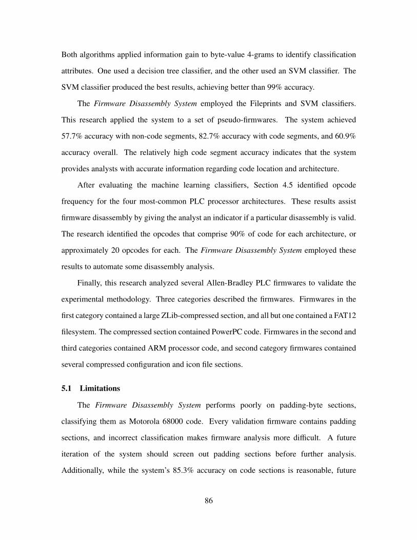
Both algorithms applied information gain to byte-value 4-grams to identify classification

attributes. One used a decision tree classifier, and the other used an SVM classifier. The

SVM classifier produced the best results, achieving better than 99% accuracy.

The Firmware Disassembly System employed the Fileprints and SVM classifiers.

This research applied the system to a set of pseudo-firmwares. The system achieved

57.7% accuracy with non-code segments, 82.7% accuracy with code segments, and 60.9%

accuracy overall. The relatively high code segment accuracy indicates that the system

provides analysts with accurate information regarding code location and architecture.

After evaluating the machine learning classifiers, Section 4.5 identified opcode

frequency for the four most-common PLC processor architectures. These results assist

firmware disassembly by giving the analyst an indicator if a particular disassembly is valid.

The research identified the opcodes that comprise 90% of code for each architecture, or

approximately 20 opcodes for each. The Firmware Disassembly System employed these

results to automate some disassembly analysis.

Finally, this research analyzed several Allen-Bradley PLC firmwares to validate the

experimental methodology. Three categories described the firmwares. Firmwares in the

first category contained a large ZLib-compressed section, and all but one contained a FAT12

filesystem. The compressed section contained PowerPC code. Firmwares in the second and

third categories contained ARM processor code, and second category firmwares contained

several compressed configuration and icon file sections.

5.1 Limitations

The Firmware Disassembly System performs poorly on padding-byte sections,

classifying them as Motorola 68000 code. Every validation firmware contains padding

sections, and incorrect classification makes firmware analysis more difficult. A future

iteration of the system should screen out padding sections before further analysis.

Additionally, while the system’s 85.3% accuracy on code sections is reasonable, future

86

iterations of the system must improve the 60.1% overall performance. Finally, the system

only incorporates three common firmware compression algorithms. Some firmwares likely

include data using other compression schemes, although this research found none.

5.2 Future Work

Several possibilities exist for future work with this system. One major hurdle that

remains during firmware analysis is identifying a code segment’s loading address. The

loading address is critical to reverse engineering when code contains jumps or branches

using absolute addressing. In that case, an analyst cannot build a function call graph

without the loading address. The loading address also enables analysts to resolve code

references to data. This research leveraged information in a symbol table, and found

a symbol table format common to at least two Allen-Bradley PowerPC PLC firmwares.

Future research might determine how common that symbol table format is, and might

identify common symbol table formats for other architectures. Manufacturers may strip

symbol tables out of firmwares before distribution, so future research should consider

other techniques for determining loading address. One such technique considers switch

conditional jump tables. Future research might investigate this method further, identifying

common jump table formats for different architectures.

This research only applied five machine learning algorithms to the reverse engineering

problem. The NCD classifier performed poorly, and future research might investigate ways

to improve its performance to better match Axelsson’s results [7]. This research found

that the code classification algorithms performed well, and future research might apply the

decision tree and SVM algorithms to the file type identification problem. Future research

might consider simplifying the system block structure by combining the file type and code

architecture classification steps. Unfortunately, the information gain attribute selection

technique incurs a time/memory tradeoff that made application to the 9-class file type

problem infeasible for this research. Future research might consider eliminating some of

87

the file types, or might combine multiple types into logical groups. Each of these research

avenues has the potential to improve the system’s overall classification accuracy.

The Firmware Disassembly System’s analysis ends with code disassembly. Future

research might expand the system, applying existing static code analysis techniques to

automate vulnerability discovery. Future research might examine techniques to compare

pristine firmware to forensically-recovered firmware. Both techniques would significantly

aid analysis of rogue firmwares, the true use case of this system. Many obstacles exist to

PLC firmware dynamic code analysis, and hardware emulation in particular, and it is also

fertile ground for future research.

The Firmware Disassembly System process applies to firmwares in general, and not

just PLC firmwares. Future research might apply a similar system to printer firmwares,

or commercial off-the-shelf (COTS) networking hardware firmwares. The security of both

device classes is relatively unexplored, yet devices from both classes are present on many

networks. Insecure printer and networking hardware firmware might act as a network back

door, or a launching point for other network attacks.

Finally, future work should automate the process of finding malicious and buggy

code within firmwares. This research designed the Firmware Disassembly System as a

preprocessor for that future system. The larger system might apply existing code analysis

tools to the code sections that the Firmware Disassembly System reveals. Automated

malware and bug detection tools would enable a firmware clearing house capable of

validating firmware security prior to installation, and would speed reaction by a critical

infrastructure (CI) computer emergency response team (CERT). Such a system would

eventually reduce CI vulnerabilities, and improve CI reliability.

Recent increases in CI system network connectivity, and advances in attacker

knowledge of firmware, necessitate faster firmware reverse engineering techniques. This

thesis applied machine learning algorithms to the firmware reverse engineering problem,

88

then developed a reverse engineering process, and implemented that process in the

Firmware Disassembly System. Critically, the Firmware Disassembly System’s automatic

disassembly and analysis permitted quick identification of PLC firmware target architecture

without possessing the PLC. The system automatically identified sections that merit

further analysis, while limiting the amount of distracting extraneous output. The Firmware

Disassembly System automatically uncompressed all firmware components and produced

the assembly-language code comprising a firmware. It completed this tedious process

considerably faster than other techniques. The combination of these qualities make the

Firmware Disassembly System unique.

89

Appendix A: Disassembly at Four Offsets

For the four architectures this research considers, bytes representing code have at least

four potential disassemblies. These correspond to initial byte offsets of zero, one, two,

or three bytes. This appendix illustrates the difficulty inherent in choosing the correct

disassembly. It provides four disassemblies of the same code section from firmware

PN-20032, one disassembly for each offset. Firmware PN-20032 contains PowerPC code.

Each disassembly for this code section contains bytes that do not resolve as valid opcodes,

and each contains bytes that do resolve as valid opcodes. This fact makes it difficult for an

analyst to immediately determine the correct disassembly. The correct disassembly results

from a three byte offset.

This appendix also provides the first twenty entries in the Firmware Disassembly

System’s opcode analysis results for each disassembly. A preponderance of popular

opcodes within a disassembly provides an analyst with a quick indicator of that

disassembly’s correctness. An opcode is popular when it is part of the group of opcodes

that comprise 90% of an architecture’s code. Table 4.19 gives the popular opcodes for

each architecture. The most frequent opcodes in offset three’s analysis are all popular, and

this is not the case for the other disassemblies. This correctly suggests that the correct

disassembly results from a three byte offset.

90

Table A.1: Offset zero disassembly

Address Byte Values Disassembly Result

2c9c8: a0 be 5c 00 lhz r5,23552(r30)

2c9cc: 00 03 fd 83 .long 0x3fd83

2c9d0: 2b f4 a6 d9 cmpli cr7,1,r20,42713

2c9d4: 86 7e 2a 00 lwzu r19,10752(r30)

2c9d8: 00 03 fe 89 .long 0x3fe89

2c9dc: 2a ec df de cmpli cr5,1,r12,57310

2c9e0: 95 47 b5 00 stwu r10,-19200(r7)

2c9e4: 00 03 fe 8f .long 0x3fe8f

2c9e8: 00 5d 5e f7 .long 0x5d5ef7

2c9ec: f5 9f 9b 00 .long 0xf59f9b00

2c9f0: 00 03 fe 94 .long 0x3fe94

2c9f4: ac 72 c9 84 lhau r3,-13948(r18)

2c9f8: 71 86 f6 00 andi. r6,r12,62976

2c9fc: 00 03 fe 9a .long 0x3fe9a

2ca00: 2f 80 e6 71 cmpwi cr7,r0,-6543

2ca04: bd da 20 00 stmw r14,8192(r26)

2ca08: 00 03 fe 9f .long 0x3fe9f

2ca0c: 89 fd c4 f4 lbz r15,-15116(r29)

2ca10: b7 a1 ed 00 sthu r29,-4864(r1)

2ca14: 00 03 fe a4 .long 0x3fea4

2ca18: bc 7d 19 34 stmw r3,6452(r29)

91

Table A.2: Offset one disassembly

Address Byte Values Disassembly Result

2c9c8: be 5c 00 00 stmw r18,0(r28)

2c9cc: 03 fd 83 2b .long 0x3fd832b

2c9d0: f4 a6 d9 86 .long 0xf4a6d986

2c9d4: 7e 2a 00 00 cmp cr4,1,r10,r0

2c9d8: 03 fe 89 2a .long 0x3fe892a

2c9dc: ec df de 95 .long 0xecdfde95

2c9e0: 47 b5 00 00 .long 0x47b50000

2c9e4: 03 fe 8f 00 .long 0x3fe8f00

2c9e8: 5d 5e f7 f5 rlwnm. r30,r10,r30,31,26

2c9ec: 9f 9b 00 00 stbu r28,0(r27)

2c9f0: 03 fe 94 ac .long 0x3fe94ac

2c9f4: 72 c9 84 71 andi. r9,r22,33905

2c9f8: 86 f6 00 00 lwzu r23,0(r22)

2c9fc: 03 fe 9a 2f .long 0x3fe9a2f

2ca00: 80 e6 71 bd lwz r7,29117(r6)

2ca04: da 20 00 00 stfd f17,0(0)

2ca08: 03 fe 9f 89 .long 0x3fe9f89

2ca0c: fd c4 f4 b7 .long 0xfdc4f4b7

2ca10: a1 ed 00 00 lhz r15,0(r13)

2ca14: 03 fe a4 bc .long 0x3fea4bc

2ca18: 7d 19 34 f7 .long 0x7d1934f7

92

Table A.3: Offset two disassembly

Address Byte Values Disassembly Result

2c9c8: 5c 00 00 03 rlwnm. r0,r0,r0,0,1

2c9cc: fd 83 2b f4 .long 0xfd832bf4

2c9d0: a6 d9 86 7e lhzu r22,-31106(r25)

2c9d4: 2a 00 00 03 cmplwi cr4,r0,3

2c9d8: fe 89 2a ec .long 0xfe892aec

2c9dc: df de 95 47 stfdu f30,-27321(r30)

2c9e0: b5 00 00 03 sthu r8,3(0)

2c9e4: fe 8f 00 5d .long 0xfe8f005d

2c9e8: 5e f7 f5 9f rlwnm. r23,r23,r30,22,15

2c9ec: 9b 00 00 03 stb r24,3(0)

2c9f0: fe 94 ac 72 .long 0xfe94ac72

2c9f4: c9 84 71 86 lfd f12,29062(r4)

2c9f8: f6 00 00 03 .long 0xf6000003

2c9fc: fe 9a 2f 80 .long 0xfe9a2f80

2ca00: e6 71 bd da .long 0xe671bdda

2ca04: 20 00 00 03 subfic r0,r0,3

2ca08: fe 9f 89 fd fnmsub. f20,f31,f7,f17

2ca0c: c4 f4 b7 a1 lfsu f7,-18527(r20)

2ca10: ed 00 00 03 .long 0xed000003

2ca14: fe a4 bc 7d fnmsub. f21,f4,f17,f23

2ca18: 19 34 f7 09 .long 0x1934f709

93

Table A.4: Offset three disassembly

Address Byte Values Disassembly Result

2c9c8: 00 00 03 fd .long 0x3fd

2c9cc: 83 2b f4 a6 lwz r25,-2906(r11)

2c9d0: d9 86 7e 2a stfd f12,32298(r6)

2c9d4: 00 00 03 fe .long 0x3fe

2c9d8: 89 2a ec df lbz r9,-4897(r10)

2c9dc: de 95 47 b5 stfdu f20,18357(r21)

2c9e0: 00 00 03 fe .long 0x3fe

2c9e4: 8f 00 5d 5e lbzu r24,23902(0)

2c9e8: f7 f5 9f 9b .long 0xf7f59f9b

2c9ec: 00 00 03 fe .long 0x3fe

2c9f0: 94 ac 72 c9 stwu r5,29385(r12)

2c9f4: 84 71 86 f6 lwzu r3,-30986(r17)

2c9f8: 00 00 03 fe .long 0x3fe

2c9fc: 9a 2f 80 e6 stb r17,-32538(r15)

2ca00: 71 bd da 20 andi. r29,r13,55840

2ca04: 00 00 03 fe .long 0x3fe

2ca08: 9f 89 fd c4 stbu r28,-572(r9)

2ca0c: f4 b7 a1 ed .long 0xf4b7a1ed

2ca10: 00 00 03 fe .long 0x3fe

2ca14: a4 bc 7d 19 lhzu r5,32025(r28)

2ca18: 34 f7 09 24 addic. r7,r23,2340

94

Table A.5: Offset zero opcode analysis

Opcode Opcode Is

Popular

Frequency in

disassembly

lwz True 0.2386

ori False 0.1144

subfic False 0.1033

mulli False 0.0828

lhz False 0.0579

lfs False 0.0530

xori False 0.0429

cmplwi False 0.0305

lis True 0.0299

stbu False 0.0231

lwzu False 0.0190

stmw False 0.0179

bl True 0.0145

stfdu False 0.0121

lhzu False 0.0118

lfsu False 0.0100

lbz False 0.0088

oris False 0.0086

b True 0.0080

cmpli False 0.0079

95

Table A.6: Offset one opcode analysis

Opcode Opcode Is

Popular

Frequency in

disassembly

rlmi False 0.0644

subfic False 0.0580

addic False 0.0533

addis True 0.0473

rlwimi False 0.0424

stfd True 0.0409

lwz True 0.0402

cmpli False 0.0295

addi True 0.0267

lfs False 0.0243

stfs False 0.0242

b True 0.0236

lwzu False 0.0218

stfsu False 0.0211

ori False 0.0200

bl True 0.0186

twi False 0.0182

lbzu False 0.0175

lfd False 0.0175

ba False 0.0169

96

Table A.7: Offset two opcode analysis

Opcode Opcode Is

Popular

Frequency in

disassembly

subfic False 0.0857

addic False 0.0707

lhzu False 0.0619

mulli False 0.0520

cmpwi True 0.0514

dozi False 0.0458

addi True 0.0310

cmpli False 0.0307

cmpi False 0.0307

addis True 0.0275

rlwimi False 0.0275

vaddubm False 0.0243

twlgti False 0.0206

cmplwi False 0.0202

tweqi False 0.0189

twi False 0.0145

stfs False 0.0137

ori False 0.0132

lwz True 0.0124

rlwinm True 0.0123

97

Table A.8: Offset three opcode analysis

Opcode Opcode Is

Popular

Frequency in

disassembly

lwz True 0.1477

stw True 0.0915

mr True 0.0838

li True 0.0768

addi True 0.0680

bl True 0.0613

lis True 0.0546

cmpwi True 0.0494

beq True 0.0464

b True 0.0344

bne True 0.0276

rlwinm True 0.0197

lbz False 0.0165

mtlr True 0.0161

ori False 0.0139

blr True 0.0136

lhz False 0.0124

add True 0.0110

cmpw True 0.0105

or False 0.0101

98

Appendix B: Opcode Frequency Analysis

This appendix lists the results of the opcode frequency analysis for 100 ELF binaries

from each of four architectures. Opcode frequency for a particular file is given by

Equation B.1. In each table, mean frequency and variance measure the mean and variance

of the opcode frequencies for individual files. Pooled frequency is from all binaries

considered as one file.

opcode frequency =number of occurrences of an opcode within a file

total opcodes in the file(B.1)

B.1 ARM Opcodes

Table B.1: Top 100 opcodes for ARM

Mnemonics Pooled Frequency Mean Frequency Variance

ldr 0.204 0.204 0.012

mov 0.176 0.151 5.460 × 10−3

add 0.096 0.075 2.796 × 10−3

bl 0.087 0.062 2.962 × 10−3

str 0.072 0.068 1.613 × 10−3

cmp 0.061 0.054 8.199 × 10−4

b 0.032 0.027 2.924 × 10−4

beq 0.030 0.031 4.513 × 10−4

bx 0.024 0.031 8.370 × 10−4

andeq 0.024 0.017 4.724 × 10−4

sub 0.020 0.016 4.595 × 10−4

bne 0.019 0.014 1.069 × 10−4

99

ldrb 0.012 0.015 3.959 × 10−4

push 0.011 0.011 6.938 × 10−5

pop 0.011 0.010 5.694 × 10−5

lsl 6.797 × 10−3 4.503 × 10−3 5.574 × 10−5

ldm 6.160 × 10−3 3.808 × 10−3 9.832 × 10−5

strb 4.328 × 10−3 2.939 × 10−3 2.253 × 10−5

movne 4.201 × 10−3 2.998 × 10−3 9.699 × 10−6

subs 4.128 × 10−3 2.883 × 10−3 1.383 × 10−5

mvn 3.726 × 10−3 2.678 × 10−3 1.481 × 10−5

rsb 3.715 × 10−3 2.462 × 10−3 1.347 × 10−5

orr 3.701 × 10−3 2.818 × 10−3 8.505 × 10−5

moveq 3.688 × 10−3 2.694 × 10−3 1.259 × 10−5

and 3.510 × 10−3 2.664 × 10−3 3.248 × 10−5

ldreq 2.564 × 10−3 2.435 × 10−3 1.240 × 10−5

ldrne 2.559 × 10−3 2.337 × 10−3 6.801 × 10−6

ble 2.529 × 10−3 1.729 × 10−3 7.280 × 10−6

lsr 2.253 × 10−3 1.638 × 10−3 1.295 × 10−5

bgt 2.186 × 10−3 1.584 × 10−3 5.758 × 10−6

tst 2.184 × 10−3 1.503 × 10−3 6.701 × 10−6

stm 2.118 × 10−3 1.416 × 10−3 5.763 × 10−6

strdeq 2.043 × 10−3 1.501 × 10−3 3.900 × 10−6

blt 1.901 × 10−3 1.435 × 10−3 5.566 × 10−6

muleq 1.862 × 10−3 1.304 × 10−3 3.746 × 10−6

ldrdeq 1.817 × 10−3 1.290 × 10−3 3.524 × 10−6

cmn 1.795 × 10−3 1.209 × 10−3 8.513 × 10−6

100

blne 1.599 × 10−3 1.165 × 10−3 4.849 × 10−6

ldrh 1.519 × 10−3 1.013 × 10−3 8.812 × 10−6

asr 1.504 × 10−3 9.891 × 10−4 4.699 × 10−6

strne 1.503 × 10−3 1.423 × 10−3 3.116 × 10−6

bhi 1.333 × 10−3 9.040 × 10−4 3.734 × 10−6

strh 1.283 × 10−3 8.581 × 10−4 4.988 × 10−6

streq 1.216 × 10−3 8.834 × 10−4 5.139 × 10−6

bic 1.198 × 10−3 1.185 × 10−3 4.174 × 10−6

bls 1.189 × 10−3 8.940 × 10−4 1.858 × 10−6

bleq 1.162 × 10−3 9.505 × 10−4 8.655 × 10−6

eor 1.122 × 10−3 8.317 × 10−4 1.394 × 10−5

bge 9.826 × 10−4 6.821 × 10−4 1.410 × 10−6

addne 9.023 × 10−4 6.169 × 10−4 1.027 × 10−6

addeq 8.209 × 10−4 6.386 × 10−4 3.628 × 10−6

adds 7.523 × 10−4 5.253 × 10−4 2.269 × 10−6

bcs 7.497 × 10−4 7.877 × 10−4 1.119 × 10−6

bcc 7.177 × 10−4 5.925 × 10−4 8.695 × 10−7

mul 7.094 × 10−4 4.603 × 10−4 1.549 × 10−6

cmpne 5.966 × 10−4 3.885 × 10−4 7.388 × 10−7

stmia 5.899 × 10−4 4.184 × 10−4 2.881 × 10−6

orrs 5.773 × 10−4 4.530 × 10−4 9.063 × 10−7

movcc 5.649 × 10−4 3.952 × 10−4 4.613 × 10−7

adc 5.278 × 10−4 3.698 × 10−4 1.933 × 10−6

stmdbhi 4.899 × 10−4 5.436 × 10−4 2.087 × 10−5

ldrsh 4.872 × 10−4 3.026 × 10−4 2.260 × 10−6

101

ands 4.834 × 10−4 3.518 × 10−4 7.610 × 10−7

bxne 4.589 × 10−4 3.537 × 10−4 4.679 × 10−7

teq 4.428 × 10−4 3.752 × 10−4 7.475 × 10−7

movle 4.333 × 10−4 2.861 × 10−4 2.997 × 10−7

movge 4.090 × 10−4 2.691 × 10−4 2.542 × 10−7

movgt 4.070 × 10−4 2.585 × 10−4 3.130 × 10−7

movlt 4.066 × 10−4 2.769 × 10−4 4.069 × 10−7

subeq 4.022 × 10−4 3.944 × 10−4 4.182 × 10−6

movcs 3.967 × 10−4 3.225 × 10−4 5.857 × 10−7

rsbs 3.799 × 10−4 2.877 × 10−4 2.493 × 10−7

mla 3.712 × 10−4 2.215 × 10−4 8.882 × 10−7

stmdami 3.647 × 10−4 4.138 × 10−4 1.184 × 10−5

svceq 3.487 × 10−4 4.284 × 10−4 1.248 × 10−5

blhi 3.468 × 10−4 3.883 × 10−4 1.051 × 10−5

stmib 3.290 × 10−4 2.600 × 10−4 2.620 × 10−7

svccc 3.258 × 10−4 2.343 × 10−4 7.766 × 10−7

bxeq 3.074 × 10−4 2.475 × 10−4 6.612 × 10−7

subcs 3.061 × 10−4 2.532 × 10−4 2.705 × 10−7

strgt 2.957 × 10−4 2.606 × 10−4 1.846 × 10−6

mvneq 2.517 × 10−4 2.118 × 10−4 1.170 × 10−6

lsrs 2.498 × 10−4 1.965 × 10−4 1.748 × 10−7

movls 2.483 × 10−4 1.735 × 10−4 1.290 × 10−7

orrne 2.436 × 10−4 1.677 × 10−4 2.580 × 10−7

ldrls 2.403 × 10−4 1.660 × 10−4 2.027 × 10−7

strbeq 2.377 × 10−4 1.950 × 10−4 3.793 × 10−7

102

strhi 2.352 × 10−4 2.384 × 10−4 2.755 × 10−6

movhi 2.345 × 10−4 1.620 × 10−4 1.136 × 10−7

orrcs 2.337 × 10−4 1.928 × 10−4 1.599 × 10−7

addls 2.314 × 10−4 1.616 × 10−4 1.840 × 10−7

lsls 2.292 × 10−4 1.867 × 10−4 2.174 × 10−7

ldmmi 2.264 × 10−4 2.505 × 10−4 4.588 × 10−6

stmdb 2.263 × 10−4 2.549 × 10−4 4.096 × 10−6

strbne 2.158 × 10−4 1.513 × 10−4 1.356 × 10−7

ldmib 2.112 × 10−4 1.900 × 10−4 2.008 × 10−7

eoreq 2.035 × 10−4 1.972 × 10−4 1.994 × 10−6

teqne 1.871 × 10−4 1.583 × 10−4 1.435 × 10−7

strheq 1.858 × 10−4 1.487 × 10−4 3.757 × 10−7

addgt 1.830 × 10−4 1.456 × 10−4 3.793 × 10−7

B.2 Motorola 68000 Opcodes

Table B.2: Top 100 opcodes for Motorola 68000

Mnemonics Pooled Frequency Mean Frequency Variance

movel 0.290 0.116 0.022

moveal 0.097 0.039 2.939 × 10−3

bsrl 0.085 0.033 2.701 × 10−3

addql 0.049 0.019 7.870 × 10−4

lea 0.042 0.017 4.936 × 10−4

clrl 0.034 0.013 3.987 × 10−4

pea 0.033 0.014 4.710 × 10−4

tstl 0.024 9.106 × 10−3 1.986 × 10−4

103

moveq 0.022 8.523 × 10−3 1.823 × 10−4

beqs 0.019 7.651 × 10−3 1.304 × 10−4

unlk 0.017 7.406 × 10−3 1.381 × 10−4

cmpl 0.017 6.295 × 10−3 9.822 × 10−5

rts 0.016 6.928 × 10−3 1.238 × 10−4

moveml 0.015 6.180 × 10−3 8.564 × 10−5

beqw 0.015 5.324 × 10−3 7.299 × 10−5

braw 0.014 5.177 × 10−3 7.327 × 10−5

jsr 0.013 5.442 × 10−3 2.790 × 10−4

bral 0.012 5.905 × 10−3 1.091 × 10−4

addl 0.011 3.964 × 10−3 6.882 × 10−5

jmp 0.011 5.215 × 10−3 8.536 × 10−5

bnes 0.010 4.275 × 10−3 4.674 × 10−5

moveb 0.010 4.059 × 10−3 1.182 × 10−4

lsll 8.356 × 10−3 2.905 × 10−3 6.086 × 10−5

bras 8.014 × 10−3 3.162 × 10−3 4.045 × 10−5

linkw 7.836 × 10−3 3.549 × 10−3 3.739 × 10−5

bnew 7.716 × 10−3 2.838 × 10−3 2.253 × 10−5

subql 7.580 × 10−3 3.095 × 10−3 3.782 × 10−5

fmoved 5.470 × 10−3 1.685 × 10−3 9.437 × 10−5

cmpal 5.320 × 10−3 2.119 × 10−3 2.496 × 10−5

subl 4.893 × 10−3 1.706 × 10−3 1.713 × 10−5

movew 4.224 × 10−3 1.472 × 10−3 4.281 × 10−5

addal 4.215 × 10−3 1.451 × 10−3 1.467 × 10−5

fmoves 3.371 × 10−3 1.063 × 10−3 9.187 × 10−5

104

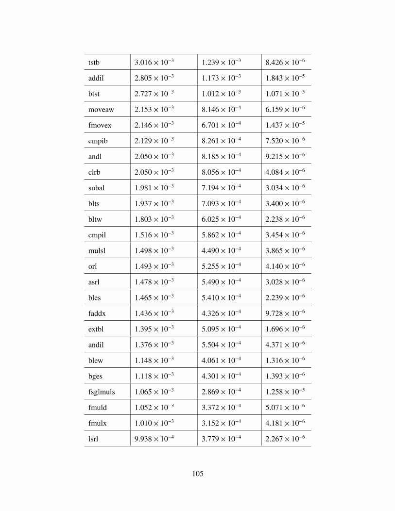
tstb 3.016 × 10−3 1.239 × 10−3 8.426 × 10−6

addil 2.805 × 10−3 1.173 × 10−3 1.843 × 10−5

btst 2.727 × 10−3 1.012 × 10−3 1.071 × 10−5

moveaw 2.153 × 10−3 8.146 × 10−4 6.159 × 10−6

fmovex 2.146 × 10−3 6.701 × 10−4 1.437 × 10−5

cmpib 2.129 × 10−3 8.261 × 10−4 7.520 × 10−6

andl 2.050 × 10−3 8.185 × 10−4 9.215 × 10−6

clrb 2.050 × 10−3 8.056 × 10−4 4.084 × 10−6

subal 1.981 × 10−3 7.194 × 10−4 3.034 × 10−6

blts 1.937 × 10−3 7.093 × 10−4 3.400 × 10−6

bltw 1.803 × 10−3 6.025 × 10−4 2.238 × 10−6

cmpil 1.516 × 10−3 5.862 × 10−4 3.454 × 10−6

mulsl 1.498 × 10−3 4.490 × 10−4 3.865 × 10−6

orl 1.493 × 10−3 5.255 × 10−4 4.140 × 10−6

asrl 1.478 × 10−3 5.490 × 10−4 3.028 × 10−6

bles 1.465 × 10−3 5.410 × 10−4 2.239 × 10−6

faddx 1.436 × 10−3 4.326 × 10−4 9.728 × 10−6

extbl 1.395 × 10−3 5.095 × 10−4 1.696 × 10−6

andil 1.376 × 10−3 5.504 × 10−4 4.371 × 10−6

blew 1.148 × 10−3 4.061 × 10−4 1.316 × 10−6

bges 1.118 × 10−3 4.301 × 10−4 1.393 × 10−6

fsglmuls 1.065 × 10−3 2.869 × 10−4 1.258 × 10−5

fmuld 1.052 × 10−3 3.372 × 10−4 5.071 × 10−6

fmulx 1.010 × 10−3 3.152 × 10−4 4.181 × 10−6

lsrl 9.938 × 10−4 3.779 × 10−4 2.267 × 10−6

105

clrw 9.822 × 10−4 3.339 × 10−4 2.638 × 10−6

bgtw 9.809 × 10−4 3.689 × 10−4 1.566 × 10−6

bgew 9.770 × 10−4 3.315 × 10−4 7.113 × 10−7

fsubx 9.406 × 10−4 2.630 × 10−4 4.472 × 10−6

negl 9.012 × 10−4 3.287 × 10−4 8.185 × 10−7

fmovel 8.524 × 10−4 3.191 × 10−4 1.930 × 10−6

bccs 8.229 × 10−4 3.250 × 10−4 9.875 × 10−7

bccw 7.345 × 10−4 2.710 × 10−4 6.021 × 10−7

bgts 7.191 × 10−4 2.791 × 10−4 6.290 × 10−7

fmovemx 6.675 × 10−4 2.461 × 10−4 8.501 × 10−7

faddd 6.475 × 10−4 2.254 × 10−4 2.218 × 10−6

swap 6.415 × 10−4 2.239 × 10−4 2.316 × 10−6

bfextu 5.953 × 10−4 2.509 × 10−4 1.930 × 10−6

subxl 5.892 × 10−4 1.955 × 10−4 7.172 × 10−7

eorl 5.607 × 10−4 2.185 × 10−4 6.544 × 10−6

rolw 5.584 × 10−4 1.844 × 10−4 6.293 × 10−6

bcsw 5.436 × 10−4 1.984 × 10−4 3.320 × 10−7

bcss 5.086 × 10−4 1.995 × 10−4 3.123 × 10−7

bhiw 4.905 × 10−4 1.826 × 10−4 6.445 × 10−7

bhis 4.900 × 10−4 2.383 × 10−4 7.891 × 10−7

cmpiw 4.871 × 10−4 1.893 × 10−4 1.432 × 10−6

fsglmulx 4.868 × 10−4 1.300 × 10−4 3.698 × 10−6

fadds 4.711 × 10−4 1.551 × 10−4 3.297 × 10−6

notb 4.599 × 10−4 2.304 × 10−4 2.173 × 10−6

oriw 4.371 × 10−4 1.481 × 10−4 5.150 × 10−7

106

fcmpx 4.358 × 10−4 1.343 × 10−4 7.121 × 10−7

sne 4.326 × 10−4 1.704 × 10−4 4.352 × 10−7

negb 4.279 × 10−4 1.675 × 10−4 6.346 × 10−7

fmovecrx 4.260 × 10−4 1.406 × 10−4 5.662 × 10−7

seq 4.242 × 10−4 1.592 × 10−4 2.551 × 10−7

blss 4.167 × 10−4 1.957 × 10−4 5.667 × 10−7

fsubs 3.926 × 10−4 9.743 × 10−5 2.093 × 10−6

fintrzx 3.565 × 10−4 1.383 × 10−4 4.447 × 10−7

fdivx 3.502 × 10−4 1.097 × 10−4 4.614 × 10−7

blsw 3.333 × 10−4 1.206 × 10−4 4.016 × 10−7

addxl 3.116 × 10−4 1.097 × 10−4 5.899 × 10−7

orib 3.044 × 10−4 1.397 × 10−4 2.177 × 10−7

rorl 2.780 × 10−4 8.583 × 10−5 1.655 × 10−6

fcmpd 2.779 × 10−4 8.750 × 10−5 2.563 × 10−7

bclr 2.707 × 10−4 9.441 × 10−5 3.968 × 10−7

notl 2.698 × 10−4 8.058 × 10−5 1.784 × 10−7

bset 2.694 × 10−4 9.131 × 10−5 3.174 × 10−7

B.3 PowerPC Opcodes

Table B.3: Top 100 opcodes for PowerPC

Mnemonics Pooled Frequency Mean Frequency Variance

lwz 0.202 0.111 0.013

mr 0.109 0.047 3.638 × 10−3

stw 0.108 0.068 5.599 × 10−3

bl 0.074 0.034 2.345 × 10−3

107

addi 0.073 0.045 2.351 × 10−3

li 0.044 0.023 7.311 × 10−4

b 0.038 0.018 5.380 × 10−4

cmpwi 0.032 0.014 3.524 × 10−4

beq 0.027 0.012 2.235 × 10−4

mtctr 0.026 0.017 4.833 × 10−4

bne 0.020 9.697 × 10−3 1.700 × 10−4

nop 0.019 8.615 × 10−3 1.369 × 10−4

mflr 0.017 9.835 × 10−3 1.552 × 10−4

bctrl 0.013 0.012 4.702 × 10−4

blr 0.013 8.461 × 10−3 1.139 × 10−4

mtlr 0.012 7.778 × 10−3 8.292 × 10−5

bctr 0.012 4.531 × 10−3 7.371 × 10−5

stwu 0.010 7.333 × 10−3 9.559 × 10−5

lis 9.770 × 10−3 0.013 7.895 × 10−4

rlwinm 9.489 × 10−3 3.524 × 10−3 5.770 × 10−5

add 8.205 × 10−3 2.879 × 10−3 5.858 × 10−5

cmpw 8.003 × 10−3 4.084 × 10−3 3.572 × 10−5

stfd 7.871 × 10−3 7.067 × 10−3 2.998 × 10−4

addis 7.860 × 10−3 3.178 × 10−3 3.096 × 10−5

bcl 7.266 × 10−3 2.724 × 10−3 2.729 × 10−5

crclr 6.774 × 10−3 4.746 × 10−3 1.052 × 10−4

lbz 6.136 × 10−3 3.941 × 10−3 1.786 × 10−4

stwcx 4.964 × 10−3 1.825 × 10−3 4.354 × 10−5

lwarx 4.564 × 10−3 1.653 × 10−3 4.216 × 10−5

108

stb 4.291 × 10−3 3.280 × 10−3 3.405 × 10−5

lfd 3.448 × 10−3 1.184 × 10−3 2.480 × 10−5

lfs 3.392 × 10−3 1.202 × 10−3 5.700 × 10−5

subf 3.209 × 10−3 1.165 × 10−3 9.922 × 10−6

ble 3.073 × 10−3 1.129 × 10−3 7.246 × 10−6

cmplw 2.683 × 10−3 1.620 × 10−3 1.148 × 10−5

blt 2.656 × 10−3 1.389 × 10−3 7.657 × 10−6

bgt 2.588 × 10−3 1.371 × 10−3 7.484 × 10−6

bge 2.273 × 10−3 1.280 × 10−3 5.075 × 10−6

addic 2.220 × 10−3 1.092 × 10−3 2.152 × 10−5

lwzx 2.023 × 10−3 6.462 × 10−4 1.021 × 10−5

cmplwi 1.807 × 10−3 1.805 × 10−3 2.347 × 10−5

clrlwi 1.786 × 10−3 8.320 × 10−4 1.253 × 10−5

srawi 1.384 × 10−3 4.760 × 10−4 3.472 × 10−6

ori 1.162 × 10−3 5.370 × 10−4 3.536 × 10−6

lhz 1.146 × 10−3 5.335 × 10−4 4.565 × 10−6

andi 1.086 × 10−3 3.824 × 10−4 2.223 × 10−6

fmr 1.062 × 10−3 3.259 × 10−4 6.725 × 10−6

mullw 1.023 × 10−3 2.847 × 10−4 2.326 × 10−6

fsub 1.005 × 10−3 3.247 × 10−4 2.998 × 10−6

sth 9.405 × 10−4 4.463 × 10−4 4.584 × 10−6

or 9.313 × 10−4 2.989 × 10−4 4.820 × 10−6

lwzu 8.468 × 10−4 5.458 × 10−4 1.762 × 10−5

stfs 8.220 × 10−4 2.412 × 10−4 8.398 × 10−6

dozi 7.581 × 10−4 5.424 × 10−4 2.884 × 10−5

109

fmul 7.353 × 10−4 2.018 × 10−4 2.158 × 10−6

fcmpu 6.459 × 10−4 1.944 × 10−4 1.237 × 10−6

andis 6.173 × 10−4 3.786 × 10−4 9.402 × 10−6

xoris 6.155 × 10−4 2.820 × 10−4 1.948 × 10−6

subfic 5.699 × 10−4 3.658 × 10−4 9.345 × 10−6

mtcrf 5.698 × 10−4 1.911 × 10−4 3.593 × 10−7

mfcr 5.549 × 10−4 2.314 × 10−4 6.434 × 10−7

twi 5.389 × 10−4 4.331 × 10−4 1.693 × 10−5

stwx 5.047 × 10−4 1.804 × 10−4 4.760 × 10−7

lfsu 5.036 × 10−4 3.590 × 10−4 1.200 × 10−5

bdnz 4.941 × 10−4 1.509 × 10−4 4.702 × 10−7

stmw 4.371 × 10−4 3.858 × 10−4 1.737 × 10−5

xor 4.319 × 10−4 1.609 × 10−4 2.251 × 10−6

lha 4.266 × 10−4 2.248 × 10−4 4.639 × 10−6

isync 4.260 × 10−4 1.851 × 10−4 1.678 × 10−6

bla 4.181 × 10−4 3.057 × 10−4 8.940 × 10−6

fadd 4.175 × 10−4 1.275 × 10−4 1.046 × 10−6

fadds 4.122 × 10−4 5.933 × 10−5 3.736 × 10−6

xori 3.862 × 10−4 1.772 × 10−4 5.411 × 10−7

fmadd 3.835 × 10−4 9.789 × 10−5 8.422 × 10−7

neg 3.727 × 10−4 1.168 × 10−4 3.035 × 10−7

fdiv 3.705 × 10−4 1.137 × 10−4 7.415 × 10−7

rlwimi 3.666 × 10−4 1.698 × 10−4 1.333 × 10−6

fsubs 3.565 × 10−4 5.150 × 10−5 3.237 × 10−6

lbzx 3.494 × 10−4 1.820 × 10−4 9.695 × 10−7

110

lwsync 3.489 × 10−4 1.483 × 10−4 1.341 × 10−6

lbzu 3.469 × 10−4 2.509 × 10−4 4.184 × 10−6

lfdx 3.433 × 10−4 9.182 × 10−5 7.644 × 10−7

oris 3.404 × 10−4 2.281 × 10−4 3.907 × 10−6

fmuls 3.230 × 10−4 5.681 × 10−5 1.146 × 10−6

fmadds 3.022 × 10−4 5.604 × 10−5 1.203 × 10−6

stbx 2.920 × 10−4 9.600 × 10−5 6.106 × 10−7

lmw 2.788 × 10−4 2.261 × 10−4 5.257 × 10−6

subfe 2.762 × 10−4 1.000 × 10−4 2.106 × 10−7

and 2.607 × 10−4 9.626 × 10−5 5.368 × 10−7

fctiwz 2.603 × 10−4 8.791 × 10−5 2.696 × 10−7

extsh 2.263 × 10−4 8.447 × 10−5 2.095 × 10−6

stfdx 2.248 × 10−4 5.552 × 10−5 3.453 × 10−7

cmpi 2.189 × 10−4 1.667 × 10−4 2.691 × 10−6

cntlzw 2.173 × 10−4 7.179 × 10−5 9.951 × 10−8

rotlwi 2.173 × 10−4 7.879 × 10−5 9.542 × 10−7

ba 1.968 × 10−4 1.482 × 10−4 2.053 × 10−6

rlwnm 1.829 × 10−4 1.411 × 10−4 1.811 × 10−6

addze 1.802 × 10−4 6.972 × 10−5 1.433 × 10−7

lhzx 1.748 × 10−4 5.453 × 10−5 1.048 × 10−7

mcrf 1.714 × 10−4 6.664 × 10−5 5.635 × 10−7

111

B.4 AVR Opcodes

Table B.4: Top 100 opcodes for AVR

Mnemonics Pooled Frequency Mean Frequency Variance

sbc 0.104 0.087 2.385 × 10−3

sbci 0.065 0.054 9.367 × 10−4

rjmp 0.065 0.054 9.958 × 10−4

ori 0.059 0.049 1.322 × 10−3

cpi 0.054 0.045 5.534 × 10−4

ldd 0.054 0.043 6.339 × 10−4

cp 0.046 0.041 1.398 × 10−3

ldi 0.040 0.031 5.693 × 10−4

sub 0.038 0.032 4.133 × 10−4

rcall 0.037 0.031 3.833 × 10−4

subi 0.036 0.030 2.620 × 10−4

andi 0.035 0.028 3.138 × 10−4

add 0.033 0.028 4.953 × 10−4

or 0.030 0.026 3.344 × 10−4

mul 0.026 0.022 3.080 × 10−4

std 0.024 0.020 1.476 × 10−4

cpc 0.021 0.018 1.791 × 10−4

in 0.018 0.014 1.343 × 10−4

adc 0.018 0.015 2.156 × 10−4

out 0.018 0.015 7.890 × 10−5

mov 0.016 0.014 2.544 × 10−4

nop 0.013 0.012 1.165 × 10−3

112

eor 0.013 0.011 5.447 × 10−5

ld 0.013 0.010 5.450 × 10−5

sbis 0.011 9.558 × 10−3 7.980 × 10−5

cbi 0.010 8.018 × 10−3 4.731 × 10−5

muls 9.442 × 10−3 8.021 × 10−3 9.234 × 10−5

and 9.347 × 10−3 7.766 × 10−3 5.623 × 10−5

cpse 9.055 × 10−3 7.506 × 10−3 2.756 × 10−5

sbic 7.840 × 10−3 6.164 × 10−3 2.548 × 10−5

sbi 7.138 × 10−3 5.929 × 10−3 2.624 × 10−5

bld 6.306 × 10−3 5.145 × 10−3 1.895 × 10−5

mulsu 5.309 × 10−3 4.491 × 10−3 4.397 × 10−5

movw 4.265 × 10−3 3.753 × 10−3 3.453 × 10−5

fmuls 4.208 × 10−3 3.677 × 10−3 1.667 × 10−5

brid 3.478 × 10−3 2.845 × 10−3 2.712 × 10−5

bst 3.036 × 10−3 2.418 × 10−3 7.188 × 10−6

sbrc 2.876 × 10−3 2.338 × 10−3 4.079 × 10−6

sbiw 2.459 × 10−3 2.145 × 10−3 1.224 × 10−5

brie 2.177 × 10−3 1.674 × 10−3 1.073 × 10−5

reti 2.175 × 10−3 1.957 × 10−3 8.058 × 10−6

sbrs 2.096 × 10−3 1.753 × 10−3 2.608 × 10−6

brtc 1.586 × 10−3 1.276 × 10−3 7.550 × 10−7

lds 1.362 × 10−3 1.178 × 10−3 1.097 × 10−6

st 1.293 × 10−3 1.035 × 10−3 1.284 × 10−6

brcs 1.125 × 10−3 9.175 × 10−4 7.523 × 10−7

adiw 9.635 × 10−4 7.981 × 10−4 8.986 × 10−7

113

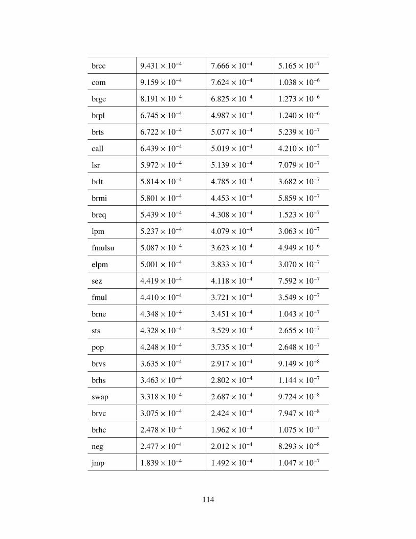
brcc 9.431 × 10−4 7.666 × 10−4 5.165 × 10−7

com 9.159 × 10−4 7.624 × 10−4 1.038 × 10−6

brge 8.191 × 10−4 6.825 × 10−4 1.273 × 10−6

brpl 6.745 × 10−4 4.987 × 10−4 1.240 × 10−6

brts 6.722 × 10−4 5.077 × 10−4 5.239 × 10−7

call 6.439 × 10−4 5.019 × 10−4 4.210 × 10−7

lsr 5.972 × 10−4 5.139 × 10−4 7.079 × 10−7

brlt 5.814 × 10−4 4.785 × 10−4 3.682 × 10−7

brmi 5.801 × 10−4 4.453 × 10−4 5.859 × 10−7

breq 5.439 × 10−4 4.308 × 10−4 1.523 × 10−7

lpm 5.237 × 10−4 4.079 × 10−4 3.063 × 10−7

fmulsu 5.087 × 10−4 3.623 × 10−4 4.949 × 10−6

elpm 5.001 × 10−4 3.833 × 10−4 3.070 × 10−7

sez 4.419 × 10−4 4.118 × 10−4 7.592 × 10−7

fmul 4.410 × 10−4 3.721 × 10−4 3.549 × 10−7

brne 4.348 × 10−4 3.451 × 10−4 1.043 × 10−7

sts 4.328 × 10−4 3.529 × 10−4 2.655 × 10−7

pop 4.248 × 10−4 3.735 × 10−4 2.648 × 10−7

brvs 3.635 × 10−4 2.917 × 10−4 9.149 × 10−8

brhs 3.463 × 10−4 2.802 × 10−4 1.144 × 10−7

swap 3.318 × 10−4 2.687 × 10−4 9.724 × 10−8

brvc 3.075 × 10−4 2.424 × 10−4 7.947 × 10−8

brhc 2.478 × 10−4 1.962 × 10−4 1.075 × 10−7

neg 2.477 × 10−4 2.012 × 10−4 8.293 × 10−8

jmp 1.839 × 10−4 1.492 × 10−4 1.047 × 10−7

114

dec 1.764 × 10−4 1.541 × 10−4 1.180 × 10−7

inc 1.181 × 10−4 9.001 × 10−5 1.272 × 10−8

push 8.242 × 10−5 6.645 × 10−5 9.349 × 10−9

asr 7.927 × 10−5 6.237 × 10−5 1.677 × 10−8

ror 6.192 × 10−5 4.858 × 10−5 6.359 × 10−9

des 3.839 × 10−5 2.886 × 10−5 2.372 × 10−9

ret 3.434 × 10−5 2.810 × 10−5 4.994 × 10−9

sec 3.327 × 10−5 1.850 × 10−5 3.804 × 10−8

cli 1.864 × 10−5 1.352 × 10−5 2.940 × 10−9

ijmp 1.395 × 10−5 1.111 × 10−5 6.020 × 10−10

spm 3.679 × 10−6 2.804 × 10−6 1.093 × 10−10

eijmp 2.648 × 10−6 1.987 × 10−6 5.490 × 10−10

seh 2.435 × 10−6 1.885 × 10−6 1.051 × 10−10

set 1.635 × 10−6 1.363 × 10−6 2.877 × 10−10

icall 1.564 × 10−6 1.347 × 10−6 6.965 × 10−11

sev 1.351 × 10−6 8.481 × 10−7 6.810 × 10−11

eicall 1.244 × 10−6 1.017 × 10−6 4.951 × 10−11

sen 1.155 × 10−6 1.169 × 10−6 8.271 × 10−11

cls 1.137 × 10−6 9.571 × 10−7 3.885 × 10−11

clt 1.120 × 10−6 8.592 × 10−7 3.774 × 10−11

clv 1.031 × 10−6 7.319 × 10−7 3.336 × 10−11

wdr 9.775 × 10−7 6.419 × 10−7 2.563 × 10−11

clc 9.242 × 10−7 7.735 × 10−7 3.412 × 10−11

clz 9.242 × 10−7 7.356 × 10−7 4.751 × 10−11

sei 9.242 × 10−7 7.487 × 10−7 4.463 × 10−11

115

cln 9.064 × 10−7 7.463 × 10−7 6.100 × 10−11

clh 8.531 × 10−7 5.739 × 10−7 2.052 × 10−11

ses 8.531 × 10−7 6.768 × 10−7 3.306 × 10−11

116

Bibliography

[1] M. Abrams and J. Weiss. Bellingham, Washington, Control System Cyber SecurityCase Study. Technical report, MITRE, August 2007. http://csrc.nist.gov/groups/SMA/fisma/ics/documents/Bellingham Case Study report%2020Sep071.pdf. 4 Feb2013.

[2] M. Abrams and J. Weiss. Malicious Control System Cyber Security At-tack Case Study – Maroochy Water Services, Australia. Case Study 08-1145, MITRE, August 2008. http://csrc.nist.gov/groups/SMA/fisma/ics/documents/Maroochy-Water-Services-Case-Study report.pdf. 4 Feb 2013.

[3] R. Akkiraju, T. Mitra, and U. Thulasiram. “Reverse Engineering PlatformIndependent Models from Business Software Applications”. Reverse Engineering- Recent Advances and Applications, 83–94. InTech Press, March 2012.

[4] I. Albert. “python-statlib: Descriptive statistics for the python programminglanguage”, December 2007. http://code.google.com/p/python-statlib/. 4 Feb 2013.

[5] M. C. Amirani et al. “A new approach to content-based file type detection”. IEEESymposium on Computers and Communications, 1103–1108. July 2008. http://dx.doi.org/10.1109/ISCC.2008.4625611. 4 Feb 2013.

[6] ARM Limited. ARM Developer Suite Version 1.2 Developer Guide. TechnicalReport ARM DUI 0056D, November 2001. http://lyle.smu.edu/∼mitch/class/5385/

ADS-Dev-Guide-DUI0056.pdf. 4 Feb 2013.

[7] S. Axelsson. “Using Normalized Compression Distance for Classifying FileFragments”. ARES ’10 International Conference on Availability, Reliability, andSecurity, 641–646. February 2010. http://dx.doi.org/10.1109/ARES.2010.100. 4 Feb2013.

[8] D. Barr. Supervisory Control and Data Acquisition (SCADA) Systems. TechnicalReport NCS TIB 04-1, National Communications System, October 2004.

[9] N. Beebe. “Digital Forensic Research: The Good, the Bad and the Unaddressed”.Gilbert Peterson and Sujeet Shenoi (editors), Advances in Digital Forensics V,volume 306 of IFIP Advances in Information and Communication Technology, 17–36. Springer Boston, 2009. http://dx.doi.org/10.1007/978-3-642-04155-6 2. 4 Feb2013.

[10] G. W. Bush. Critical infrastructure identification, prioritization, and protection.Homeland Security Presidential Directive HSPD-7, White House, Washington,December 2003. http://www.dhs.gov/homeland-security-presidential-directive-7#1.4 Feb 2013.

117

[11] E. Byres, A. Ginter, and J. Langill. How Stuxnet Spreads - A Study of Infection Pathsin Best Practice Systems. Technical report, Tofino Security, 2011.

[12] W. C. Calhoun and D. Coles. “Predicting the types of file fragments”. DigitalInvestigation, 5S(0):S14–S20, September 2008. http://www.sciencedirect.com/

science/article/pii/S1742287608000273. 4 Feb 2013.

[13] W. J. Clinton. Critical Infrastructure Protection. Presidential Decision DirectivePDD-63, White House, Washington, May 1998. http://www.fas.org/irp/offdocs/pdd/

pdd-63.htm. 4 Feb 2013.

[14] CompuServe Incorporated. GIF: Graphics Interchange Format. Technical Reportgif87a, June 1987. http://www.w3.org/Graphics/GIF/spec-gif87.txt. 4 Feb 2013.

[15] G. Conti et al. “Automated mapping of large binary objects using primitive fragmenttype classification”. Digital Investigation, 7S(0):S3–S12, August 2010. http://www.sciencedirect.com/science/article/pii/S1742287610000290. 4 Feb 2013.

[16] B. Copy and F. Tilaro. “Standards based measurable security for embeddeddevices”. Proceedings of the 12th International Conference on Accelerator and LargeExperimental Physics Control Systems. October 2009.

[17] A. Cutts. “Warfare and the Continuum of Cyber Risks: A Policy Perspective”. TheVirtual Battlefield: Perspectives on Cyber Warfare, 66–76. IOS Press, 2009.

[18] I. Dacosta et al. “Security Analysis of an IP Phone: Cisco 7960G”. HenningSchulzrinne et al. (editors), Principles, Systems and Applications of IP Telecommu-nications. Services and Security for Next Generation Networks, 236–255. Springer-Verlag, Berlin, Heidelberg, 2008. http://dx.doi.org/10.1007/978-3-540-89054-6 12.4 Feb 2013.

[19] G. Delugre. “Closer to Metal: Reverse engineering the Broadcom NetExtreme’sFirmware”, October 2010. http://esec-lab.sogeti.com/dotclear/public/publications/10-hack.lu-nicreverse slides.pdf. 4 Feb 2013.

[20] P. Deutsch. GZIP file format specification version 4.3. Request for Comments 1952,Network Working Group, May 1996. http://tools.ietf.org/html/rfc1952. 4 Feb 2013.

[21] P. Deutsch and J.-L. Gailly. ZLIB Compressed Data Format Specification version3.3. Request for Comments 1950, Network Working Group, May 1996. http://tools.ietf.org/html/rfc1950. 4 Feb 2013.

[22] D. Douglas and T. Peucker. “Algorithms for the reduction of the number ofpoints required to represent a digitized line or its caricature”. Cartographica: TheInternational Journal for Geographic Information and Geovisualization, 10(2):112–122, 1973.

118

[23] R. F. Erbacher and J. Mulholland. “Identification and localization of data types withinlarge-scale file systems”. Systematic Approaches to Digital Forensic Engineering,2007. SADFE 2007. Second International Workshop on, 55–70. IEEE, 2007.

[24] N. Falliere, L. O. Murchu, and E. Chien. W32.Stuxnet Dossier. Technical report,Symantec, February 2011.

[25] S. Fogie. “Embedded reverse engineering: Cracking mobile binaries”. CodeBreakersMagazine, 1(1), January 2006.

[26] Free Software Foundation. “GNU Binutils”, August 2007. http://www.gnu.org/

software/binutils/. 4 Feb 2013.

[27] S. Garfinkel et al. “Bringing Science to Digital Forensics with Standardized ForensicCorpora”. Digital Investigation, 6:S2–S11, 2009.

[28] J. Grand. “Introduction to embedded security”, July 2004. http://www.blackhat.com/

presentations/bh-usa-04/bh-us-04-grand/grand embedded security US04.pdf. 4 Feb2013.

[29] T. Hurman. Exploring Windows CE shellcode. Technical report, Pentest Limited,June 2005.

[30] International Business Machines. PowerPC Microprocessor Family: The Pro-gramming Environments for 32-Bit Microprocessors. Technical Report G522-0290-01, February 2000. https://www-01.ibm.com/chips/techlib/techlib.nsf/techdocs/852569B20050FF778525699600719DF2/%24file/6xx pem.pdf. 4 Feb 2013.

[31] International Electrotechnical Commission. IEC61131-3 - Programmable Controllers- Part 3: Programming Languages. International Electrotechnical Commission,Geneva, second edition, January 2003.

[32] M. Karresand and N. Shahmehri. “File Type Identification of Data Fragments byTheir Binary Structure”. Information Assurance Workshop, 2006 IEEE, 140–147.June 2006. http://dx.doi.org/10.1109/IAW.2006.1652088. 4 Feb 2013.

[33] M. Karresand and N. Shahmehri. “Oscar - File Type Identification of Binary Datain Disk Clusters and RAM Pages”. Fischer-Hubner et al. (editors), Security andPrivacy in Dynamic Environments, volume 201 of IFIP International Federation forInformation Processing, 413–424. Springer Boston, 2006. http://dx.doi.org/10.1007/

0-387-33406-8 35. 4 Feb 2013.

[34] J. Kleinberg and E. Tardos. Algorithm Design. Addison-Wesley, 2006.

[35] J. Z. Kolter and M. A. Maloof. “Learning to Detect and Classify MaliciousExecutables in the Wild”. Journal of Machine Learning Research, 7:2721–2744,December 2006. http://dl.acm.org/citation.cfm?id=1248547.1248646. 4 Feb 2013.

119

[36] W. J. Li et al. “Fileprints: identifying file types by n-gram analysis”. Proceedingsfrom the Sixth Annual IEEE SMC Information Assurance Workshop, 2005, 64–71.June 2005. http://dx.doi.org/10.1109/IAW.2005.1495935. 4 Feb 2013.

[37] A. Matrosov et al. Stuxnet under the microscope. Technical report, eset Security,September 2010.

[38] R. C. Mayer. Filetype Identification Using Long, Summarized n-Grams. Master’sthesis, Naval Postgraduate School, Monterey, CA, March 2011. http://www.dtic.mil/docs/citations/ADA543322. 4 Feb 2013.

[39] R. H. McClanahan. “SCADA and IP: is network convergence really here?” IndustryApplications Magazine, IEEE, 9(2):29–36, March 2003. http://dx.doi.org/10.1109/

MIA.2003.1180947. 4 Feb 2013.

[40] M. McDaniel and M. H. Heydari. “Content Based File Type Detection Algorithms”.Proceedings of the 36th Annual Hawaii International Conference on System Sciences.IEEE, January 2003. http://ieeexplore.ieee.org/xpl/login.jsp?&arnumber=1174905. 4Feb 2013.

[41] L. R. McMinn. External Verification of SCADA System Embedded ControllerFirmware. Master’s thesis, Air Force Inst of Tech, Wright-Patterson AFB, OH,Graduate School of Engineering and Management, March 2012. http://oai.dtic.mil/oai/oai?verb=getRecord&metadataPrefix=html&identifier=ADA557800. 4 Feb2013.

[42] “Melissa virus creator jailed”. BBC Americas, 2 May 2002. http://news.bbc.co.uk/2/

hi/americas/1963371.stm. 4 Feb 2013.

[43] C. Miller. Battery Firmware Hacking: Inside the innards of a Smart Battery.Technical report, Accuvant Labs, July 2011.

[44] S. J. Moody and R. F. Erbacher. “SADI-statistical analysis for data typeidentification”. Systematic Approaches to Digital Forensic Engineering, 2008.SADFE’08. Third International Workshop on, 41–54. IEEE, 2008.

[45] NewMedia-NET. “dd-wrt — Unleash your Router”, January 2013. http://www.dd-wrt.com/site/index. 4 Feb 2013.

[46] A. Pal and N. Memon. “The evolution of file carving”. Signal Processing Magazine,IEEE, 26(2):59–71, March 2009. http://dx.doi.org/10.1109/MSP.2008.931081. 4 Feb2013.

[47] I. Pavlov. “7-Zip”, October 2012. http://www.7-zip.org/. 4 Feb 2013.

[48] D. Peck and D. Peterson. “Leveraging Ethernet Card Vulnerabilities in FieldDevices”. SCADA Security Scientific Symposium, 1–19. Digital Bond, 2009.

120

[49] J. Platt. “Fast training of support vector machines using sequential minimaloptimization”. B. Scholkopf, C.J.C. Burges, and A.J. Smola (editors), Advances inKernel Methods—Support Vector Learning. MIT Press, August 1998.

[50] Python Software Foundation. “random — Generate pseudo-random numbers”,January 2013. http://docs.python.org/3.3/library/random.html. 4 Feb 2013.

[51] J. R. Quinlan. C4.5: Programs for machine learning. Morgan Kaufmann, 1993.http://bit.ly/WpUp5n. 4 Feb 2013.

[52] G. G. Richard and V. Roussev. “Scalpel: A Frugal, High Performance File Carver”.Proceedings of the 2005 digital forensics research workshop (DFRWS 2005). 2005.

[53] P. Roberts. “Hacker Says Texas Town Used Three Character Password To SecureInternet Facing SCADA System”. ThreatPost, November 2011. http://bit.ly/unkgYg.4 Feb 2013.

[54] Rockwell Automation. “CompactLogix System”, January 2013. http://www.ab.com/en/epub/catalogs/12762/2181376/2416247/407648/7921736/

CompactLogix-Modular-Systems.html. 4 Feb 2013.

[55] Rockwell Automation. “Network Resources”, January 2013. http://www.rockwellautomation.com/support/networks/overview.page. 4 Feb 2013.

[56] A. W. Samuel. Hacktivism and the Future of Political Participation. Ph.D. thesis,Harvard University, Cambridge MA, September 2004.

[57] I. Schnell. “bitarray 0.8.0: Efficient arrays of booleans – C extension”, April 2012.http://pypi.python.org/pypi/bitarray/. 4 Feb 2013.

[58] M. D. Schwartz et al. Control System Devices: Architectures and Supply ChannelsOverview. Technical Report SAND2010-5183, Sandia National Laboratories, August2010.

[59] Siemens Automation. “SIMATIC WinCC”, June 2012. http://www.automation.siemens.com/mcms/human-machine-interface/en/visualization-software/scada/

simatic-wincc/Pages/Default.aspx. 4 Feb 2013.

[60] R. L. Sites et al. “Binary translation”. Commun. ACM, 36(2):69–81, February 1993.http://doi.acm.org/10.1145/151220.151227. 4 Feb 2013.

[61] M. Story and R. G. Congalton. “Accuracy assessment - A user’s perspective”.Photogrammetric Engineering and remote sensing, 52(3):397–399, March 1986.

[62] K. Stouffer, J. Falco, and K. Kent. Guide to Supervisory Control and Data Acquisition(SCADA) and Industrial Control Systems Security. Technical Report SpecialPublication 800-82, National Institute of Standards and Technology, September 2006.

121

[63] The OpenWrt Developers. “OpenWrt”, November 2012. https://openwrt.org/. 4 Feb2013.

[64] The Rockbox Crew. “Rockbox - Free Music Player Firmware”, January 2013.http://www.rockbox.org/. 4 Feb 2013.

[65] J. Thilmany. “SCADA Security?” Mechanical Engineering, 25–31, June 2012.

[66] “Under Cyberthreat: Defense Contractors”. Bloomberg Businessweek, 6 July 2009.http://buswk.co/Wn3jif. 4 Feb 2013.

[67] W. Underwood. “Grammar-Based Specification and Parsing of Binary File Formats”.The International Journal of Digital Curation, 7(1):95–106, March 2012.

[68] United States Computer Emergency Readiness Team. ICS-Alert: Control SystemInternet Accessibility. Technical Report 10-301-01, October 2010.

[69] United States Computer Emergency Readiness Team and National Institute ofStandards and Technology. Vulnerability Summary for CVE-2010-2965. CommonVulnerabilities and Exposures CVE-2010-2965, August 2010. http://web.nvd.nist.gov/view/vuln/detail?vulnId=CVE-2010-2965. 4 Feb 2013.

[70] United States Computer Emergency Readiness Team and National Institute ofStandards and Technology. Vulnerability Summary for CVE-2012-0929. CommonVulnerabilities and Exposures CVE-2012-0929, January 2012. http://web.nvd.nist.gov/view/vuln/detail?vulnId=CVE-2012-0929. 4 Feb 2013.

[71] United States Computer Emergency Readiness Team and National Institute ofStandards and Technology. Vulnerability Summary for CVE-2012-0931. CommonVulnerabilities and Exposures CVE-2012-0931, January 2012. http://web.nvd.nist.gov/view/vuln/detail?vulnId=CVE-2012-0931. 4 Feb 2013.

[72] United States Computer Emergency Readiness Team and National Institute ofStandards and Technology. Vulnerability Summary for CVE-2012-4690. CommonVulnerabilities and Exposures CVE-2012-4690, December 2012. http://web.nvd.nist.gov/view/vuln/detail?vulnId=CVE-2012-4690. 4 Feb 2013.

[73] United States Computer Emergency Readiness Team and National Institute ofStandards and Technology. Vulnerability Summary for CVE-2012-5049. CommonVulnerabilities and Exposures CVE-2012-5049, September 2012. http://web.nvd.nist.gov/view/vuln/detail?vulnId=CVE-2012-5049. 4 Feb 2013.

[74] C. Veenman. “Statistical Disk Cluster Classification for File Carving”. InformationAssurance and Security, 2007. IAS 2007. Third International Symposium on, 393–398. IEEE, August 2007. http://dx.doi.org/10.1109/IAS.2007.75. 4 Feb 2013.

122

[75] R. P. Weicker. “Dhrystone: a synthetic systems programming benchmark”. Commun.ACM, 27(10):1013–1030, October 1984. http://doi.acm.org/10.1145/358274.358283.4 Feb 2013.

[76] Wind River. “Wind River VxWorks”, January 2013. http://www.windriver.com/

products/vxworks.html. 4 Feb 2013.

[77] I. Witten and E. Frank. Data Mining: Practical machine learning tools andtechniques. Morgan Kaufmann, 2005. http://www.cs.waikato.ac.nz/∼ml/weka/. 4Feb 2013.

[78] Y. Yang and J. O. Pedersen. “A Comparative Study on Feature Selection in TextCategorization”. Proceedings of the Fourteenth International Conference on MachineLearning, 412–420. Morgan Kaufmann, San Francisco, 1997.

[79] A. Yasinsac et al. Software Review and Security Analysis of the ES&S iVotronic 8.0.1.2Voting Machine Firmware. Technical report, Florida State University, February2007. http://www.electioncenter.org/documents/2007/FinalReportSAITLab.pdf. 4Feb 2013.

[80] L. Zhang and G. B. White. “An Approach to Detect Executable Content forAnomaly Based Network Intrusion Detection”. Parallel and Distributed ProcessingSymposium, 2007. IPDPS 2007. IEEE International, 1–8. March 2007. http://dx.doi.org/10.1109/IPDPS.2007.370614. 4 Feb 2013.

[81] C. Zoulas. “file(1) - Linux Man Page”, October 2008. http://linux.die.net/man/1/file.4 Feb 2013.

123

REPORT DOCUMENTATION PAGE Form ApprovedOMB No. 0704–0188

The public reporting burden for this collection of information is estimated to average 1 hour per response, including the time for reviewing instructions, searching existing data sources, gathering andmaintaining the data needed, and completing and reviewing the collection of information. Send comments regarding this burden estimate or any other aspect of this collection of information, includingsuggestions for reducing this burden to Department of Defense, Washington Headquarters Services, Directorate for Information Operations and Reports (0704–0188), 1215 Jefferson Davis Highway,Suite 1204, Arlington, VA 22202–4302. Respondents should be aware that notwithstanding any other provision of law, no person shall be subject to any penalty for failing to comply with a collectionof information if it does not display a currently valid OMB control number. PLEASE DO NOT RETURN YOUR FORM TO THE ABOVE ADDRESS.

1. REPORT DATE (DD–MM–YYYY) 2. REPORT TYPE 3. DATES COVERED (From — To)

4. TITLE AND SUBTITLE 5a. CONTRACT NUMBER

5b. GRANT NUMBER

5c. PROGRAM ELEMENT NUMBER

5d. PROJECT NUMBER

5e. TASK NUMBER

5f. WORK UNIT NUMBER

6. AUTHOR(S)

7. PERFORMING ORGANIZATION NAME(S) AND ADDRESS(ES) 8. PERFORMING ORGANIZATION REPORTNUMBER

9. SPONSORING / MONITORING AGENCY NAME(S) AND ADDRESS(ES) 10. SPONSOR/MONITOR’S ACRONYM(S)

11. SPONSOR/MONITOR’S REPORTNUMBER(S)

16. SECURITY CLASSIFICATION OF:

a. REPORT b. ABSTRACT c. THIS PAGE

17. LIMITATION OFABSTRACT

18. NUMBEROFPAGES

19a. NAME OF RESPONSIBLE PERSON

19b. TELEPHONE NUMBER (include area code)

Standard Form 298 (Rev. 8–98)Prescribed by ANSI Std. Z39.18

21–03–2013 Master’s Thesis Oct 2011–Mar 2013

File Carving and Malware Identification Algorithms Applied toFirmware Reverse Engineering

Sickendick, Karl A., Captain, USAF

Air Force Institute of TechnologyGraduate School of Engineering and Management (AFIT/EN)2950 Hobson WayWPAFB, OH 45433-7765

AFIT-ENG-13-M-46

Department of Homeland Security ICS-CERTPOC: Neil Hershfield, DHS ICS-CERT Technical LeadATTN: NPPD/CS&C/NCSD/US-CERTMailstop: 0635, 245 Murray Lane, SW, Bldg 410, Washington DC 20528Email: ics-cert@dhs.gov; Phone: 1-877-776-7585

DHS ICS-CERT

12. DISTRIBUTION / AVAILABILITY STATEMENT

DISTRIBUTION STATEMENT A. APPROVED FOR PUBLIC RELEASE; DISTRIBUTION UNLIMITED

13. SUPPLEMENTARY NOTES

This work is declared a work of the U.S. Government and is not subject to copyright protection in the United States.

14. ABSTRACT

Modern society depends on critical infrastructure (CI) managed by Programmable Logic Controllers (PLCs). PLCsdepend on firmware, though firmware security vulnerabilities and contents remain largely unexplored. Attackers areacquiring the knowledge required to construct and install malicious firmware on CI. To the defender, firmware reverseengineering is a critical, but tedious, process.This thesis applies machine learning algorithms, from the file carving and malware identification fields, to firmwarereverse engineering. It characterizes the algorithms’ performance. This research describes and characterizes a process tospeed and simplify PLC firmware analysis. The system partitions binary firmwares into segments, labels each segmentwith a file type, determines the target architecture of code segments, then disassembles and performs rudimentaryanalysis on the code segments.The research discusses the system’s accuracy on a set of pseudo-firmwares. Of the algorithms this research considers,a combination of a byte-value frequency file carving algorithm and a support vector machine (SVM) algorithm usinginformation gain (IG) for feature selection achieve the best performance. That combination correctly identifies the filetypes of 57.4% of non-code bytes, and the architectures of 85.3% of code bytes. This research applies the FirmwareDisassembly System to a real-world firmware and discusses the contents.

15. SUBJECT TERMS

Control systems, firmware, reverse engineering, programmable logic controller (PLC)

U U U UU 137

Thomas, E. Dube, Maj, USAF

(937) 255-3636 ext. 4613