atlab simulator for adaptive filters - diva portal829400/fulltext01.pdfmatlab simulator for adaptive...

MATLAB SIMULATOR FOR ADAPTIVE FILTERS

Submitted by:

Raja Abid Asghar

- BS Electrical Engineering (Blekinge Tekniska Högskola, Sweden)

Abu Zar

- BS Electrical Engineering (Blekinge Tekniska Högskola, Sweden)

Supervisor:

Mr. Muhammad Shahid

- PhD fellow in Applied Signal Processing (Blekinge Tekniska Högskola, Sweden)

Examiner:

Dr. Sven Johansson

- Department of Electrical Engineering, School of Engineering (Blekinge Tekniska Högskola, Sweden)

http://www.bth.se/

http://www.bth.se/

http://www.bth.se/

http://www.bth.se/

Abstract

Adaptive filters play an important role in modern day signal processing with applications such as

noise cancellation, signal prediction, adaptive feedback cancellation and echo cancellation. The

adaptive filters used in our thesis, LMS (Least Mean Square) filter and NLMS (Normalized Least

Mean Square) filter, are the most widely used and simplest to implement. The application we

tested in our thesis is noise cancellation. A detail study of both filters is done by taking into

account different cases. Broadly test cases were divided into two categories of stationary signal

and non-stationary signal to observe performance against the type of signal involved. Noise

variance was another factor that was considered to learn its effect. Also parameters of adaptive

filter, such as step size and filter order, were varied to study their effect on performance of

adaptive filters. The results achieved through these test cases are discussed in detail and will help

in better understanding of adaptive filters with respect to signal type, noise variance and filter

parameters.

Acknowledgment

We would like to acknowledge the contributions made by our teachers for building our basic

knowledge and skills in the field of engineering. Then we would especially like to thank our

supervisor Mr. Shahid for his support and continuous guidance without which it would not have

been possible to complete this project. We would like to thank our parents and siblings for their

love and care always and we would like to thank our friends for their support and help.

Contents

Chapter 1. Introduction to Signal Processing .................................................................................. 1

1.1. Transversal FIR Filters ............................................................................................................ 1

1.2. Random Signals ..................................................................................................................... 3

1.3. Correlation Function .............................................................................................................. 3

1.4. Stationary Signals .................................................................................................................. 4

1.5. Non-Stationary Signals .......................................................................................................... 5

Chapter 2. Introduction to Adaptive Filters ..................................................................................... 7

2.1. Introduction ........................................................................................................................... 7

2.2. Wiener Filters ........................................................................................................................ 8

2.3. Mean Square Error (MSE) Adaptive Filters ........................................................................... 9

Chapter 3. Least Mean Square Algorithm ..................................................................................... 10

3.1. Introduction ......................................................................................................................... 10

3.2. Derivation of LMS Algorithm ............................................................................................... 10

3.3. Implementation of LMS Algorithm ...................................................................................... 12

3.4. Computational Efficiency of LMS ........................................................................................ 13

Chapter 4. Normalized Least Mean Square Algorithm .................................................................. 14

4.1. Introduction ......................................................................................................................... 14

4.2. Derivation of NLMS Algorithm ............................................................................................ 15

4.3. Implementation of NLMS Algorithm ................................................................................... 16

4.4. Computational Efficiency of LMS ........................................................................................ 16

Chapter 5. Introduction to Matlab Simulator ................................................................................ 18

5.1. Input Selection .................................................................................................................... 19

5.2. Algorithm Selection ............................................................................................................. 19

5.3. Algorithm Stop Criteria ........................................................................................................ 19

5.4. Desired Output Signal.......................................................................................................... 20

5.5. Output of Filter .................................................................................................................... 20

5.6. Error Plot and its Importance .............................................................................................. 20

5.7. Learning Curve ..................................................................................................................... 21

5.8. Filter Coefficient Plot ........................................................................................................... 21

5.9. Frequency Response Plot .................................................................................................... 21

5.10. Final Execution ................................................................................................................. 21

Chapter 6. Results and Analysis Of Stationary Signals ................................................................... 22

6.1. Stationary Signal with Noise at all Frequencies .................................................................. 22

6.1.1. Observing the LMS filter response for different step sizes ......................................... 22

6.1.2. Observing the LMS filter response for different filter order ....................................... 25

6.1.3. Observing the NLMS filter response for different step sizes ....................................... 26

6.1.4. Observing the NLMS filter response for different filter order ..................................... 28

6.1.5. Comparing LMS with NLMS for same filter order and step size .................................. 30

6.1.6. Comparison of LMS and NLMS for variation in noise .................................................. 33

6.2. Stationary Signal with Noise at High Frequencies Only ...................................................... 36

6.2.1. Observing the LMS filter response for different step sizes ......................................... 36

6.2.2. Observing the LMS filter response for different filter order ....................................... 38

6.2.3. Observing the NLMS filter response for different step sizes ....................................... 40

6.2.4. Observing the NLMS filter response for different filter order ..................................... 42

6.2.5. Comparing LMS with NLMS for same filter order and step size .................................. 43

6.2.6. Comparison of LMS and NLMS for variation in noise .................................................. 47

Chapter 7. Result and Analysis of Non-Stationary Signals ............................................................. 50

7.1. Non-Stationary Signal with Sinousidal Noise ...................................................................... 50

7.1.1. Results of LMS filter ..................................................................................................... 50

7.1.2. Results of NLMS filter ................................................................................................... 54

7.2. Non-Stationary Signal With Random Noise ........................................................................ 57

7.2.1. Results of LMS filter ..................................................................................................... 57

7.2.2. Results of NLMS filter ................................................................................................... 61

Chapter 8. Conclusion .................................................................................................................... 65

References.......................................................................................................................................... 67

MATLAB Simulator for Adaptive Filters

Page 1

Chapter 1. Introduction to Signal Processing

Real world signals are analog and continuous, e.g: an audio signal, as heard by our ears is a

continuous waveform which derives from air pressure variations fluctuating at frequencies which

we interpret as sound. However, in modern day communication systems these signals are

represented electronically by discrete numeric sequences. In these sequences, each value

represents an instantaneous value of the continuous signal. These values are taken at regular time

periods, known as the sampling period, Ts. [1]

For example, consider a continuous waveform given by x(t). In order to process this waveform

digitally we first must convert this into a discrete time vector. Each value in the vector represents

the instantaneous value of this waveform at integer multiples of the sampling period. The values

of the sequence, x(t) corresponding to the value at n times the sampling period is denoted as x(n).

𝑥(𝑛) = 𝑥(𝑛𝑇�) → 𝑒𝑞𝑢𝑎𝑡𝑖𝑜𝑛 1.1

1.1. Transversal FIR Filters A filter can be defined as a piece of software or hardware that takes an input signal and processes

it so as to extract and output certain desired elements of that signal (Diniz 1997, p.1)[2]. There are

numerous filtering methods, both analog and digital which are widely used. However, this thesis

shall be contained to adaptive filtering using a particular method known as transversal finite

impulse response (FIR) filters. The characteristics of a transversal FIR filter can be expressed as a

vector consisting of values known as tap weights. It is these tap weights which determine the

performance of the filter. These values are expressed in the column vector form as, w(n) = [w0(n)

w1(n) w2(n) …. wN-1(n)]T. This vector represents the impulse response of the FIR filter. The number

of elements in this vector is N which is the order of the filter. [1]

The utilization of an FIR filter is simple, the output of the FIR filter at a time sample ‘n’ is

determined by the sum of the products between the tap weight vector, w(n) and N time delayed


Page 2

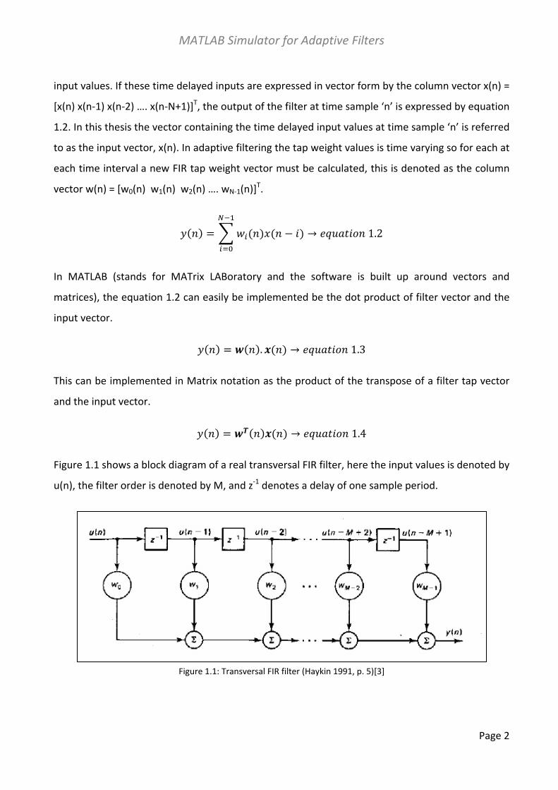
input values. If these time delayed inputs are expressed in vector form by the column vector x(n) =

[x(n) x(n-1) x(n-2) …. x(n-N+1)]T, the output of the filter at time sample ‘n’ is expressed by equation

1.2. In this thesis the vector containing the time delayed input values at time sample ‘n’ is referred

to as the input vector, x(n). In adaptive filtering the tap weight values is time varying so for each at

each time interval a new FIR tap weight vector must be calculated, this is denoted as the column

vector w(n) = [w0(n) w1(n) w2(n) …. wN-1(n)]T.

𝑦(𝑛) = �𝑤�(𝑛)𝑥(𝑛 − 𝑖)��

��

→ 𝑒𝑞𝑢𝑎𝑡𝑖𝑜𝑛 1.2

In MATLAB (stands for MATrix LABoratory and the software is built up around vectors and

matrices), the equation 1.2 can easily be implemented be the dot product of filter vector and the

input vector.

𝑦(𝑛) = 𝒘(𝑛).𝒙(𝑛) → 𝑒𝑞𝑢𝑎𝑡𝑖𝑜𝑛 1.3

This can be implemented in Matrix notation as the product of the transpose of a filter tap vector

and the input vector.

𝑦(𝑛) = 𝒘𝑻(𝑛)𝒙(𝑛) → 𝑒𝑞𝑢𝑎𝑡𝑖𝑜𝑛 1.4

Figure 1.1 shows a block diagram of a real transversal FIR filter, here the input values is denoted by

u(n), the filter order is denoted by M, and z-1 denotes a delay of one sample period.

Figure 1.1: Transversal FIR filter (Haykin 1991, p. 5)[3]


Page 3

Adaptive filters utilize algorithms to iteratively alter the values of the filter tap vector in order to

minimize a value known as the cost function. The cost function, 𝜉(n), is a function of the difference

between a desired output and the actual output of the FIR filter. This difference is known as the

estimated error of the adaptive filter, e(n) = d(n)-y(n) . This is explained in detail in the chapter 2.

1.2. Random Signals A random signal, expressed by a random variable function, x(t), does not have a precise

description of its waveform. It may, however, be possible to express these random processes by

statistical or probabilistic models (Diniz 1997, p.17)[2]. A single occurrence of a random variable

appears to behave unpredictably. But if we take several occurrences of the variable, each denoted

by n, then the random signal is expressed by two variables, x(t,n).

The main characteristic of a random signal known as the expectation of a random signal is defined

as the mean value across all n occurrences of that random variable, denoted by E[x(t)], where x(t)

is the input random variable. In this Project the expectation of an input signal is equal to the

actual value of that signal. However, the E[x(n)] notation shall still be used in order to derive the

various algorithms used in adaptive filtering which will be discussed later.

1.3. Correlation Function The correlation function is a measure of how statistically similar two functions are. The

autocorrelation function of a random signal is defined as the expectation of a signal value at time

n multiplied by its complex conjugate value at a different time m. This is shown in equation 1.5, for

time arbitrary time instants, n and m.

𝜑��(𝑛,𝑚) = 𝐸[𝑥(𝑛)𝑥∗(𝑚)] → 𝑒𝑞𝑢𝑎𝑡𝑖𝑜𝑛 1.5

If real signal is used, as in the case of our project, than then equation 1.5 can be expressed as:

𝜑��(𝑛,𝑚) = 𝐸[𝑥(𝑛)𝑥(𝑚)] → 𝑒𝑞𝑢𝑎𝑡𝑖𝑜𝑛 1.6


Page 4

The derivations of adaptive filtering algorithms utilize the autocorrelation matrix, R. For real

signals this is defined as the matrix of expectations of the product of a vector x(n)and its

transpose. This is shown in equation 1.7 (Diniz 1997, p27)[2].

𝑹 = 𝐸[𝒙(𝑘)𝒙�(𝑘)] → 𝑒𝑞𝑢𝑎𝑡𝑖𝑜𝑛 1.7

The autocorrelation matrix has the additional property that its trace, i.e. the sum of its diagonal

elements, is equal to the sum of the powers of the values in the input vector (Farhang-Boroujeny

1999, p. 97)[4]. As we will see later, sometimes a single value replaces one of the vectors in the

autocorrelation matrix, in this case the correlation function results in a vector. This vector is given

by the expectation of that single value multiplied by the expectation of each of the values in the

vector.

Correlation matrices and vectors are based on either cross-correlation or autocorrelation

functions. In cross correlation the signals are different and in autocorrelation same signal is used.

1.4. Stationary Signals A signal is considered stationary in the wide sense, if the following two criteria are fulfilled

(Farhang-Boroujeny 1999, pp 37-8) [4].

The mean values, or expectations, of the signal are constant for any shift in time.

𝑚�(𝑛) = 𝑚�(𝑛 + 𝑘) → 𝑒𝑞𝑢𝑎𝑡𝑖𝑜𝑛 1.8

The autocorrelation function is also constant over an arbitrary time shift.

𝜑��(𝑛,𝑚) = 𝜑��(𝑛 + 𝑘,𝑚 + 𝑘) → 𝑒𝑞𝑢𝑎𝑡𝑖𝑜𝑛 1.9

The above implies that the statistical properties of a stationary signal are constant over time. In

the derivation of adaptive filtering algorithms it is often assumed that the signal input to the


Page 5

algorithm are stationary. Speech signals are not stationary in the wide sense however they do

exhibit some temporary stationary behaviour as will be discussed later.

1.5. Non-Stationary Signals A non-stationary signal is one whose frequency change over time; e.g. speech where frequencies

vary over time. A speech signal consists of three classes of sounds. They are voiced, fricative and

plosive sounds. Voiced sounds are caused by excitation of the vocal tract with quasi-periodic

pulses of airflow. Fricative sounds are formed by constricting the vocal tract and passing air

through it, causing turbulence which results in a noise-like sound. Explosive sounds are created by

closing up the vocal tract, building up air behind it and then suddenly releasing it. This is heard in

the sound made by the letter ‘p’ (Oppenheim and Schafer 1989, p. 724)[5].

Figure 1.2: Example of Speech Signal


Page 6

Figure 1.2 shows a discrete time representation of a speech signal. By looking at it as a whole we

can tell that it is non-stationary. That is, its mean values vary with time and cannot be predicted

using the above mathematical models for random processes. However, a speech signal can be

considered as a linear composite of the above three classes of sound, each of these sounds are

stationary and remain fairly constant over intervals of the order of 30 to 40 ms (Oppenheim and

Schafer 1989, p. 724)[5].

The theory behind the derivations of many adaptive filtering algorithms usually requires the input

signal to be stationary. Although speech is non-stationary for all time, it is an assumed in this

project that the short term stationary behaviour outlined above will prove adequate for the

adaptive filters to function as desired.


Page 7

Chapter 2. Introduction to Adaptive Filters

2.1. Introduction Figure 2.1 shows the block diagram of the adaptive filter method.

Figure 2.1. Adaptive filter block diagram (Farhang-Boroujeny 1999, p. 120)[4]

Here w represents the coefficients of the FIR filter tap weight vector, x(n) is the input vector

samples, z-1 is a delay of one sample period, y(n) is the adaptive filter output, d(n) is the desired

signal and e(n) is the estimation error at time n. The aim of an adaptive filter is to calculate the

difference between the desired signal and the adaptive filter output, e(n) which is called error

signal and is fed back into the adaptive filter and its coefficients are changed algorithmically in

order to minimize a function of this difference, known as the cost function. When the adaptive

filter output is equal to desired signal the error signal goes to zero.

The two adaptive filtering methods used in this project are known as Mean Square Error (MSE)

adaptive filters. They aim to minimize a cost function equal to the expectation of the square of the


Page 8

difference between the desired signal d(n), and the actual output of the adaptive filter y(n). This is

shown in equation 2.1.

𝜉(𝑛) = 𝐸[𝑒�(𝑛)] = 𝐸[(𝑑(𝑛) − 𝑦(𝑛))�] → 𝑒𝑞𝑢𝑎𝑡𝑖𝑜𝑛 2.1

2.2. Wiener Filters Wiener filters are a special class of transversal FIR filters which builds upon the means square

error cost function of equation 2.1 to arrive at an optimal filter tap weight vector which reduces

the MSE signal to a minimum. They will be used in the derivation of adaptive filtering algorithms in

later sections, this theory is based on Diniz 1997, pp. 38 to 42 [2], and Farhang-Boroujeny 1999,

pp. 51-54 [4].

Consider the output of the transversal FIR filter as given below, for a filter tap weight vector, w(n),

and input vector, x(n).

𝑦(𝑛) = �𝑤�(𝑛)𝑥(𝑛 − 𝑖)��

��

= 𝒘𝑻(𝑛)𝒙(𝑛) → 𝑒𝑞𝑢𝑎𝑡𝑖𝑜𝑛 2.2

The mean square error cost function can be expressed in terms of the cross-correlation vector

between the desired and input signals, p(n) = E[ x(n) d(n) ], and the autocorrelation matrix of the

input signal, R(n) = E[ x(n) xT(n) ].

𝜉(𝑛) = 𝐸[𝑒�(𝑛)]

𝜉(𝑛) = 𝐸[(𝑑(𝑛) − 𝑦(𝑛))�]

𝜉(𝑛) = 𝐸[𝑑�(𝑛) − 2𝑑(𝑛)𝒘𝑻(𝑛)𝒙(𝑛) + 𝒘𝑻(𝑛)𝒙(𝑛)𝒙𝑻(𝑛)𝒘(𝑛)]

𝜉(𝑛) = 𝐸[𝑑�(𝑛)] − 2𝐸[𝒘𝑻(𝑛)𝒙(𝑛)𝑑(𝑛)] + 𝐸[𝒘𝑻(𝑛)𝒙(𝑛)𝒙𝑻(𝑛)𝒘(𝑛)]

𝜉(𝑛) = 𝐸[𝑑�(𝑛)] − 2𝒘𝑻𝒑 + 𝒘𝑻𝑹𝒘 → 𝑒𝑞𝑢𝑎𝑡𝑖𝑜𝑛 2.3


Page 9

When applied to FIR filtering the above cost function is an N-dimensional quadratic function. The

minimum value of 𝜉(n) can be found by calculating its gradient vector related to the filter tap

weights and equating it to 0.

By finding the gradient of equation 2.3, equating it to zero and rearranging gives us the optimal

Wiener solution for the filter tap weights, wo.

∇𝜉 = 0

0 − 2𝒑 + 𝟐𝑹𝒘𝒐 = 𝟎

𝒘𝒐 = 𝑹��𝒑 → 𝑒𝑞𝑢𝑎𝑡𝑖𝑜𝑛 2.4

The optimal Wiener solution is the set of filter tap weights which reduce the cost function to zero.

This vector can be found as the product of the inverse of the input vector autocorrelation matrix

and the cross correlation vector between the desired signal and the input vector. The Least

Mean Square algorithm of adaptive filtering attempts to find the optimal Wiener solution using

estimations based on instantaneous values.

2.3. Mean Square Error (MSE) Adaptive Filters Mean Square Error (MSE) adaptive filters, they aim to minimize a cost function equal to the

expectation of the square of the difference between the desired signal d(n), and the actual output

of the adaptive filter y(n). The cost function is defined by equation:

𝜉(𝑛) = 𝐸[𝑒�(𝑛)] = 𝐸[(𝑑(𝑛) − 𝑦(𝑛))�]

The two types algorithms for mean square error filters which are discussed in this thesis are:

I. Least mean square (LMS) algorithm (Chapter 3)

II. Normalized Least mean square (NLMS) algorithm (Chapter 4)


Page 10

Chapter 3. Least Mean Square Algorithm

3.1. Introduction The Least Mean Square (LMS) algorithm was first developed by Widrow and Hoff in 1959 through

their studies of pattern recognition (Haykin 1991, p. 67) [3]. From there it has become one of

the most widely used algorithms in adaptive filtering. The LMS algorithm is a type of adaptive filter

known as stochastic gradient-based algorithms as it utilizes the gradient vector of the filter tap

weights to converge on the optimal Wiener solution. It is well known and widely used due to its

computational simplicity. It is this simplicity that has made it the benchmark against which all

other adaptive filtering algorithms are judged (Haykin 1991, p. 299) [3].

The filter tap weights of the adaptive filter are updated in every iteration of algorithm according to

the following formula (Farhang-Boroujeny 1999, p. 141)[4].

𝒘(𝑛 + 1) = 𝒘(𝑛) + 2𝜇𝑒(𝑛)𝒙(𝑛) → 𝑒𝑞𝑢𝑎𝑡𝑖𝑜𝑛 3.1

Here x(n) is the input vector of time delayed input values, x(n) = [ x(n) x(n-1) x(n-2) ….x(n-N+1) ]T.

The vector w(n) = [ w0(n) w1(n) w2(n) …. wN-1(n) ]T represents the coefficients of the adaptive FIR

filter tap weight vector at time n. The parameter µ is known as the step size parameter and is a

small positive constant. This step size parameter controls the influence of the updating factor.

Selection of a suitable value for µ is imperative to the performance of the LMS algorithm, if the

value is too small the time the adaptive filter takes to converge to the optimal solution will be too

long and if µ is too large the adaptive filter becomes unstable and its output diverges.

3.2. Derivation of LMS Algorithm The derivation of the LMS algorithm builds upon the theory of the Wiener solution for the optimal

filter tap weights, wo, as outlined in Section 2.2. It also depends on the steepest-descent algorithm

as stated in equation 3.2 and 3.3, this is a formula which updates the filter coefficients using the


Page 11

current tap weight vector and the current gradient of the cost function with respect to the filter

tap weight coefficient vector, ∇𝜉(n).

𝒘(𝑛 + 1) = 𝒘(𝑛) − 𝜇∇𝜉 → 𝑒𝑞𝑢𝑎𝑡𝑖𝑜𝑛 3.2

𝜉(𝑛) = 𝐸[𝑒�(𝑛)] → 𝑒𝑞𝑢𝑎𝑡𝑖𝑜𝑛 3.3

As the negative gradient vector points in the direction of steepest descent for the N-dimensional

quadratic cost function, each recursion shifts the value of the filter coefficients closer toward their

optimum value, which corresponds to the minimum achievable value of the cost function,

ξ(n). This derivation is based on Diniz 1997, pp.71-3 and Farhang-Boroujeny 1999, pp.139–41 [2]

[4].

The LMS algorithm is a random process implementation of the steepest descent algorithm, from

equation 3.3. Here the expectation for the error signal is not known so the instantaneous value is

used as an estimate. The steepest descent algorithm gives the cost function as in equation 3.4.

𝜉(𝑛) = 𝑒�(𝑛) → 𝑒𝑞𝑢𝑎𝑡𝑖𝑜𝑛 3.4

The gradient of the cost function, ∇𝜉(n), can alternatively be expressed in the following form.

∇𝜉(𝑛) = ∇� 𝑒�(𝑛)�

∇𝜉(𝑛) =𝜕 𝑒�(𝑛)𝜕𝒘

∇𝜉(𝑛) = 2𝑒(𝑛)𝜕𝑒(𝑛)𝜕𝒘

∇𝜉(𝑛) = 2𝑒(𝑛)𝜕(𝑑(𝑛) − 𝑦(𝑛))

𝜕𝒘


Page 12

∇𝜉(𝑛) = −2𝑒(𝑛)𝜕𝒘�(𝑛)𝒙(𝑛)

𝜕𝒘

∇𝜉(𝑛) = −2𝑒(𝑛)𝒙(𝑛) → 𝑒𝑞𝑢𝑎𝑡𝑖𝑜𝑛 3.5

Substituting this into the steepest descent algorithm of equation 3.2, we arrive at the recursion for

the LMS adaptive algorithm.


3.3. Implementation of LMS Algorithm There are three steps involved in every iteration of LMS algorithm. The order of these steps is:

i. The output of the FIR filter, y(n) is calculated using equation 3.7.

𝑦(𝑛) = �𝑤(𝑛)𝑥(𝑛 − 𝑖)��

��


ii. The value of the error estimation is calculated using equation 3.8.

𝑒(𝑛) = 𝑑(𝑛) − 𝑦(𝑛) → 𝑒𝑞𝑢𝑎𝑡𝑖𝑜𝑛 3.8

iii. The tap weights of the FIR vector are updated in preparation for the next iteration by

equation 3.9.



Page 13

3.4. Computational Efficiency of LMS The main reason for the LMS algorithm’s popularity in adaptive filtering is its computational

simplicity, making it easier to implement than all other commonly used adaptive algorithms. For

each iteration, the LMS algorithm requires 2N additions and 2N+1 multiplications (N for calculating

the output, y(n), one for 2µe(n) and an additional N for the scalar by vector multiplication)

(Farhang-Boroujeny 1999, p. 141) [4].


Page 14

Chapter 4. Normalized Least Mean Square Algorithm

4.1. Introduction One of the primary disadvantages of the LMS algorithm is having a fixed step size parameter

during whole execution. This requires an understanding of the statistics of the input signal prior to

commencing the adaptive filtering operation. Signals are not normally known before even if we

assume the only signal to be input to the adaptive noise cancellation system is speech, there are

still many factors such as signal input power and amplitude which will affect its performance.

The normalized least mean square algorithm (NLMS) is an extension of the LMS algorithm which

bypasses this issue by selecting a different step size value, µ(n), for each iteration of the algorithm.

This step size is proportional to the inverse of the total expected energy of the instantaneous

values of the coefficients of the input vector x(n) (Farhang-Boroujeny 1999, p.172) [4]. This sum of

the expected energies of the input samples is also equivalent to the dot product of the input

vector with itself, and the trace of input vectors auto-correlation matrix, R (Farhang-Boroujeny

1999, p.173) [4].

𝑡𝑟[𝑹] = �𝐸[𝑥�(𝑛 − 1)]��

��

𝑡𝑟[𝑹] = 𝐸 �� 𝑥�(𝑛 − 1)��

��

� → 𝑒𝑞𝑢𝑎𝑡𝑖𝑜𝑛 4.1

The recursion formula for the NLMS algorithm is stated in equation 4.2.

𝒘(𝑛 + 1) = 𝒘(𝑛) +1

𝒙�(𝑛)𝒙(𝑛)𝑒(𝑛)𝒙(𝑛) → 𝑒𝑞𝑢𝑎𝑡𝑖𝑜𝑛 4.2


Page 15

4.2. Derivation of NLMS Algorithm This derivation of the normalized least mean square algorithm is based on Farhang-Boroujeny

1999, pp.172-175,[4] and Diniz 1997, pp 150-3 [2]. To derive the NLMS algorithm we consider the

standard LMS recursion, for which we select a variable step size parameter,

µ(n). This parameter is selected such that the error value, e+(n), will be minimized using the

updated filter tap weights, w(n+1), and the current input vector, x(n).

𝒘(𝑛 + 1) = 𝒘(𝑛) + 2𝜇𝑒(𝑛)𝒙(𝑛)

𝑒�(𝑛) = 𝑑(𝑛) −𝒘�(𝑛 + 1)𝒙(𝑛)

𝑒�(𝑛) = �1 − 2𝜇𝑒(𝑛)𝒙�(𝑛)𝒙(𝑛)�𝑒(𝑛) → 4.3

Next we minimize (e+ (n))2 , with respect to µ(n). Using this we can then find a value for µ(n) which

forces e+(n) to zero.

𝜇(𝑛) =1

2𝒙�(𝑛)𝒙(𝑛)→ 𝑒𝑞𝑢𝑎𝑡𝑖𝑜𝑛 4.4

This µ(n) is then substituted into the standard LMS recursion replacing µ, resulting in the

following.

𝒘(𝑛 + 1) = 𝒘(𝑛) + 2𝜇𝑒(𝑛)𝒙(𝑛)

𝒘(𝑛 + 1) = 𝒘(𝑛) +1

𝒙�(𝑛)𝒙(𝑛)𝑒(𝑛)𝒙(𝑛) → 𝑒𝑞𝑢𝑎𝑡𝑖𝑜𝑛 4.5

Often the NLMS algorithm is expressed as equation 4.6, this is a slight modification of the standard

NLMS algorithm detailed above. Here the value of 𝜓 is a small positive constant in order to avoid

division by zero when the values of the input vector are zero. The parameter µ is a constant step

size value used to alter the convergence rate of the NLMS algorithm, it is within the range of 0< µ

<2, usually being equal to 1. We have used one such value throughout the MATLAB

implementations.


Page 16

𝒘(𝑛 + 1) = 𝒘(𝑛) +𝜇

𝒙�(𝑛)𝒙(𝑛) + 𝜓𝑒(𝑛)𝒙(𝑛) → 𝑒𝑞𝑢𝑎𝑡𝑖𝑜𝑛 4.6

4.3. Implementation of NLMS Algorithm As the NLMS is an extension of the standard LMS algorithm, the NLMS algorithms practical

implementation is very similar to that of the LMS algorithm. Each iteration of the NLMS algorithm

requires these steps in the following order (Farhang-Boroujeny1999, p. 175) [4].

i. The output of the adaptive filter is calculated.

𝑦(𝑛) = �𝑤(𝑛)𝑥(𝑛 − 𝑖)��

��


ii. An error signal is calculated as the difference between the desired signal and the filter

output.

𝑒(𝑛) = 𝑑(𝑛) − 𝑦(𝑛) → 𝑒𝑞𝑢𝑎𝑡𝑖𝑜𝑛 4.8

iii. The step size value is calculated from the input vector.

𝜇(𝑛) =𝜇

𝒙�(𝑛)𝒙(𝑛) + 𝜓→ 𝑒𝑞𝑢𝑎𝑡𝑖𝑜𝑛 4.9

iv. The filter tap weights are updated in preparation for the next iteration.

𝒘(𝑛 + 1) = 𝒘(𝑛) + 𝜇(𝑛)𝑒(𝑛)𝒙(𝑛) → 𝑒𝑞𝑢𝑎𝑡𝑖𝑜𝑛 4.10

4.4. Computational Efficiency of LMS Each iteration of the NLMS algorithm requires 3N+1 multiplications, this is only N more than the

standard LMS algorithm and this is an acceptable increase considering the gains in stability and

results achieved.


Page 17

The NLMS algorithm shows far greater stability with unknown signals. This combined with good

convergence speed and relative computational simplicity makes the NLMS algorithm ideal for the

real time adaptive noise cancellation system since in speech signal are unknown signals.


Page 18

Chapter 5. Introduction to Matlab Simulator

The MATLAB simulator designed in this project is shown in Figure 5.1. The ‘GUIDE’ tool of MATLAB

was used for the design of this simulator. The code for this simulator is appended in appendix

‘Code A-4’. The different sections of the simulator are numbered from 1 to 10. They are explained

below.

Figure 5.1: An outlook of the designed MATLAB simulator


Page 19

5.1. Input Selection The input section in Figure 5.1 is shown by the number 1. In this section the first two inputs are

stationary signals, a sinusoid is used in our project. The difference between the two stationary

input signals is that the first one is corrupted with noise at all frequencies while the second one is

corrupted using only high frequency noise. If one of these two inputs is selected during simulation,

then one has to provide the input signal length in the text box at the bottom of the input section.

The simulator uses this length to generate a sine signal (stationary) which becomes the desired

signal and then the signal is mixed with noise depending upon the type of selection which is input

to filter.

The last two options are for non-stationary signals with two different kinds of noise option: one

with noise at all frequencies and second with sinusoidal noise at a specific frequency. These two

selections offer the ability to load any signal file in .MAT format of the hard disk. Test speech

signals are placed with the codes of the project for loading while using this option. The speech

signal is taken as the desired signal while updating filter coefficients and the same signal when

added with noise is fed as input to the filter.

5.2. Algorithm Selection This section is shown by the number 2 in Figure 5.1. In this section there are two options of filter

selection LMS and NLMS. After selecting the filter type then we have to give value of the step size

(µ) and filter order (N) which are required for the algorithm simulation. The step size determines

the updating speed of filter coefficients. This input option of step size and filter order allows the

user to observe the filter performance on different parameters.

5.3. Algorithm Stop Criteria The algorithm stop criteria input is shown by the number 3 in Figure 5.1. This criterion tells the

algorithm to stop which means it will stop updating the filter coefficients and consider the last

filter coefficient for later filtering process without updating. If criterion is not met throughout the


Page 20

simulation or is set to be zero, then the algorithm will keep active all the time. In this project the

criterion is set at a minimum error value of user choice such that if for any 20 consecutive

iterations the absolute error is below that minimum error the criterion is met and algorithm stops.

Minimum error entered in the stop criteria input must be non-negative and should be near or

equal to zero.

5.4. Desired Output Signal The desired output signal d(n) is shown in Figure 5.1 by the number 4. It is the signal that we want

the output of the filter to be. The LMS and NLMS algorithm try to alter the filter coefficients such

that the output of the filter is close to the desired output.

5.5. Output of Filter The output of the filter y(n) is the signal that is the result of the dot multiplication input vector x(n)

and weight vector w(n) and is shown in Figure 5.1 by the number 5. It is titled estimated output as

it is a close estimate of desired signal d(n).

5.6. Error Plot and its Importance The Error plot in the Figure 5.1 is shown by the number 6. The error plot is the difference of

desired signal d(n) and filter output y(n). This difference tells us how close is the filter in producing

the desired signal, lower the absolute value of error closer the output of the filter gets to the

desired signal. The algorithm LMS and NLMS are also designed and updated according this error

value. The error plot gives us an idea how well the filter is performing.


Page 21

5.7. Learning Curve The learning curve is indicated by the number 7 on Figure 5.1. The learning curve is also an

indicator plot for filter performance. It is a plot of squared errors, both LMS and NLMS algorithms’

cost function is a function of squared errors. Also it gives a clear distinction between the transient

and steady state response of the filter.

5.8. Filter Coefficient Plot The filter coefficient plot is a plot of all the coefficient values during each iteration while

execution. The filter coefficients achieve steady state when filter converges. The plot of Figure 5.1

is shown by the number 8.

5.9. Frequency Response Plot To observe the filter type and performance it is necessary to observe its frequency response to

know the frequencies of signal which were allowed to pass. The frequency response indicated by

the number 9 exists in Figure 5.1.

5.10. Final Execution The final execution button on the simulator is to execute the code and get the result once the

inputs are entered and options are selected. The button runs the algorithm and displays all the

results on the figures indicated in Figure 5.1 and it is pointed by the number 10.

To perform a simulation first the type of input signal needs to select, then the algorithm selection

is done and parameters required are entered and at the end the error stop criterion is entered.

The final execution button displaying ‘Run the algorithm and display the result’ is pressed to

obtain all the results.


Page 22

Chapter 6. Results and Analysis Of Stationary Signals

In this chapter the simulator is used for applying adaptive filters on stationary signals. A sinousial

signal is used as a stationary signal. Two different types of noise are added to have the two test

cases.

6.1. Stationary Signal with Noise at all Frequencies The stationary signal used is a sinusoidal signal with frequency, F = 400 Hz and sampled at

sampling frequency, Fs = 12000 and is the desired signal in this case. The noise added to the input

signal is random noise present at all frequencies. Initially the noise taken is a normal distributed

data with a mean value of 0 (zero) and a standard deviation of 0.05. The adaptive filter should be

able to make a filter such that it filters out the sinusoidal frequency at angular frequency, f =

0.067π. We will observe the filter and its behaviour for the following cases:

6.1.1. Observing the LMS filter response for different step size

6.1.2. Observing the LMS Filter response for different filter orders

6.1.3. Observing the NLMS Filter response for different step sizes

6.1.4. Observing the NLMS Filter response for different filter orders

6.1.5. Comparing LMS with NLMS for same filter order and step size

6.1.6. Comparison of LMS and NLMS for variation in noise

6.1.1. Observing the LMS filter response for different step sizes

In this case the length of the input signal is 500 samples, the stop criteria are set at 0.001, the filter

order at 15, filter type is LMS and three different step sizes of 0.05 (Red), 0.025 (Blue) and 0.005

(Green) are used. The results are shown below in Figure 6.1, 6.2 and 6.3.


Page 23

Figure 6.1 shows the plot of estimated output. The results show that lower the step slower is the

convergence of the estimated output towards desired output. Green plot with the smallest step

size appears to be the slowest in convergence.

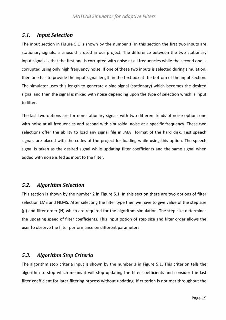
Figure 6.2 is the error plot and it shows large variation in the transient for the smallest step size

but as soon as it enters the steady state the variation also gets stable. This shows that the smaller

step size approaches steady state late but has a good response in steady state.

Figure 6.3 shows the frequency response of the finally designed filter. The result matches with our

expectation of a pass band filter to pass the desired signal. The frequency response in the pass

band for the three step sizes is almost the same but in the stop band the smaller step size results

in more attenuation of noise. The pass band is not as narrow as it should have been but it depends

on the order of the filter and not on step size.

Figure 6.1: Estimated Output, observing the LMS for different Step Sizes


Page 24

Figure 6.2: Error Plot, observing the LMS for different Step Sizes

Figure 6.3: Frequency Response, observing the LMS for different Step Sizes


Page 25

6.1.2. Observing the LMS filter response for different filter order

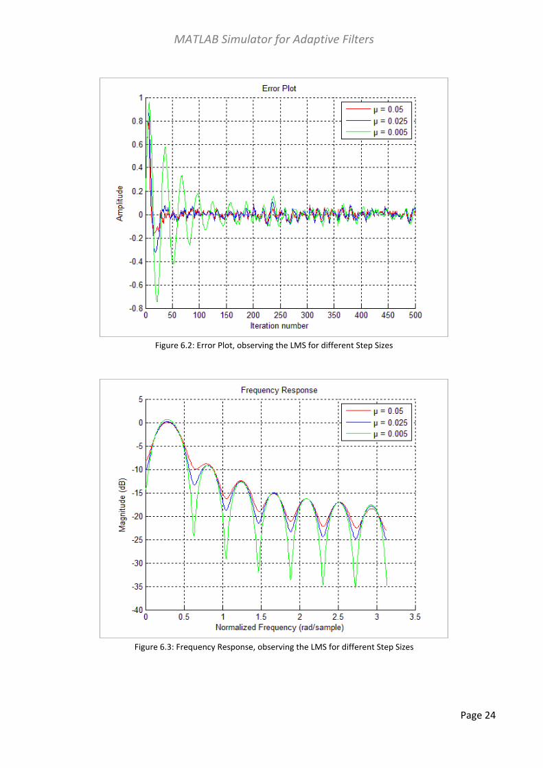
In this case the signal length is 500, the step size used is 0.02 and the three different filter orders

being tested are 15, 50 and 100. It was necessary to observe the LMS filter response to the change

in filter order. The results are shown by two Figures 6.4 and 6.5, since we can see that most of the

information about performance can be derived from error plot and frequency response.

Figure 6.4 shows the error plots for the three filter orders. The response in the transient portion is

almost the same as all three take equal time to enter the steady state. In the steady state the

response of higher filter order results in good response since the variation of the filter with low

order of 15 (Red) has a comparatively high variation.

Figure 6.5 which shows the frequency response shows a set of pass band filters against the three

filter orders. We can see that raising the filter order improves the filter response the response of

filter order 50,100 is better than 15 in the passband but is almost same for both order 50 and 100.

The response of filter with order 50 and 100 in the passband is much narrower than the filter

order 15 which also explains the reason of variation in Figure 6.4 by filter order of 15.

Figure 6.4: Error plot, observing the LMS filter response for different filter order


Page 26

Figure 6.5: Frequency response, observing the LMS filter response for different filter order

6.1.3. Observing the NLMS filter response for different step sizes

In this case the signal length is taken as 500, the filter order is 15 and three different step sizes are

used: 0.05, 0.025 and 0.01. The need was to observe the NLMS filter under variation of step size to

notice the effects. The results are shown by the error plot and frequency response and the two

plots are shown in Figure 6.6 and 6.7 respectively.

The increase in step size results in faster convergence which can be seen in Figure 6.6. If we

compare this with the same scenario for LMS which was discussed in 6.1.1., then we will see that

overall NLMS takes more time to converge but the variation is much controlled and less than LMS.

Since for NLMS the convergence time is more but with greater stability we can use higher step

sizes for NLMS as compared to the LMS.

Figure 6.7 which shows the frequency response indicate that raising step size has no effect of on

the pass band response of the filter. We see better attenuation in stop band for smaller step size

but considering the greater convergence time it takes the advantage seems to be really less.


Page 27

Figure 6.6: Error Plot, observing the NLMS filter response for different step sizes

Figure 6.7: Frequency response, observing the NLMS filter response for different step sizes


Page 28

6.1.4. Observing the NLMS filter response for different filter order

In this case the signal length is taken as 500, the step size used is 0.02 and the three different filter

orders are used: 15, 50 and 100. It was necessary to observe the NLMS filter response to the

change in filter order. The results are shown by error plot and frequency response and the two

plots are shown in Figure 6.8 and 6.9 respectively.

Figure 6.8 shows the error plot the response shows that the tracking ability and the convergence

time is almost same. The higher filter order shows very less variation after converging while the

variation in error signal of filter order of 15 is comparatively higher.

Figure 6.9 which shows the frequency response indicate that raising the filter order improves the

filter response. The filter response shows that it is trying to extract a single frequency component

as it was required and expected. The pass band gets much narrower as we raise the filter order.

During the same comparison for LMS in section 6.1.2 we saw the response for filter order 50 and

100 are almost same and better than the filter order 15. In this case of NLMS we can clearly see

the frequency response of filter order 100 is even better than the filter order of 50 and pass band

is much narrower.


Page 29

Figure 6.8: Error Plot, observing the NLMS filter response for different filter order

Figure 6.9: Frequency response, observing the NLMS filter response for different filter order


Page 30


After considering different scenarios for LMS and NLMS we need to make a comparison LMS and

NLMS to evaluate both under the same conditions.

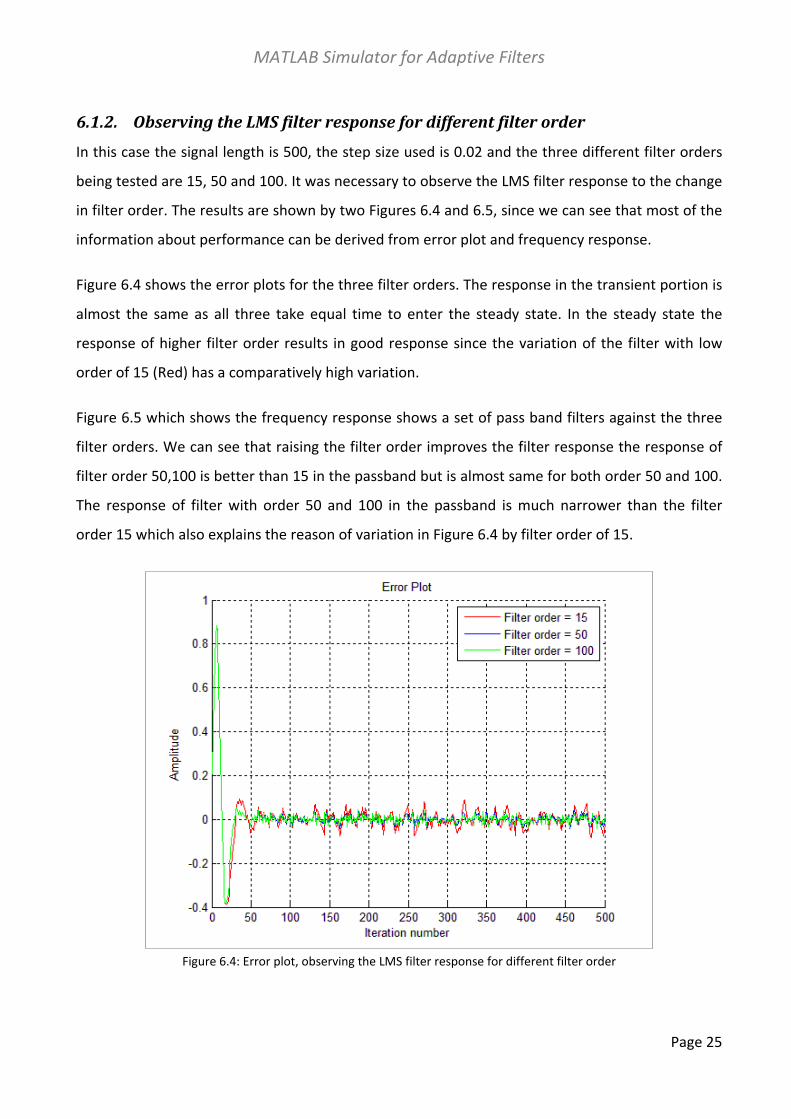
For this comparison a sinusoidal signal of length 500 is taken, Noise signal is a normal distributed

data with a mean value of 0 (zero) and a standard deviation of 0.05, the step size used is 0.025 and

the filter order used is 100. After simulation results are shown by four figures which are estimated

output plot, error plot, frequency response and learning curve which are shown in Figure 6.10,

6.11, 6.12 and 6.13 respectively.

Figure 6.10 shows the estimated plot by both LMS and NLMS. We see that NLMS take more time

for estimation than LMS. After estimation both signals look similar, we can see this after 350th

iteration. So we can deduce that NLMS is comparatively slower in convergence than LMS.

Figure 6.10: Estimated output of LMS and NLMS filter


Page 31

Figure 6.11: Error plot of LMS and NLMS filter

Figure 6.12: Frequency response of LMS and NLMS filter


Page 32

Figure 6.13: Learning curve of LMS and NLMS filter

Figure 6.11 shows the error plots for both filters. It can be observed in the error plot too that the

convergence rate of NLMS is slower than LMS. Another Figure 6.13 showing the learning curve

also gives the same result. The three figures provided us information about the speed of

convergence but for the performance of both filters after convergence we will take a look at the

frequency response plot.

The frequency response plot in Figure 6.12 shows interestingly that the filter by NLMS is much

narrower than LMS which is required for better filtering of the sinusoid. If we consider the input

signal and desired signal, we know that the desired filter should be a narrow pass band. This

shows us that the final form of filter formed by NLMS is much better than LMS as per required

condition.


Page 33


The amount of noise by which the input signal is corrupted also has an important impact on

performance of the adaptive filters and we will try to understand its role in this section. In this

scenario we will vary the amount of input noise by changing the variance of noise data. Since

variance is the square of standard deviation so we can consider different values of standard

deviation for testing. The three different values of standard deviation of noise data taken are 0.05,

0.1 and 0.2. Results are shown in Figures 6.14, 6.15, 6.16 and 6.17.

Figure 6.14: Error Plots, Effect of noise variation on LMS and NLMS


Page 34

Figure 6.15: Frequency Response Plots, Effect of noise variation on LMS and NLMS

Figure 6.14 shows the error plots for both LMS and NLMS filters and the variance of the noise is

changed. For the LMS filter we notice that the fluctuation of the error signal in the steady state is

higher as the noise standard deviation increases. For the NLMS it seems like the error signal

almost follow the same pattern for the three noise signals with rise in value of the signal. This tells

us that NLMS behaves same to the three noises.

Figure 6.15 shows the frequency response plot for both filters as we change the noise variance.

The passband characteristics of both filters, LMS and NLMS, remain almost same. The filter made

by LMS changes mostly in stop band with change in noise variance while that of NLMS almost

remains the same. This shows that NLMS behaviour towards change in noise variance remains

consistent. One possible reason of this can be the normalizing of input signal in case of NLMS. The

noise is present in the input signal and NLMS normalizing that signal, so not effecting the filter

performance.

Now if we like to come to a conclusion that which one works better we take a look on the

remaining two results of this section. Those results are shown in Figure 6.16 and 6.17. The results

indicate one previously observed conclusion that LMS has faster convergence than NLMS. If we

see the comparative results of LMS and NLMS we will see that as the noise variance increase the

steady state performance of NLMS becomes better than LMS. The reason for this can be seen in


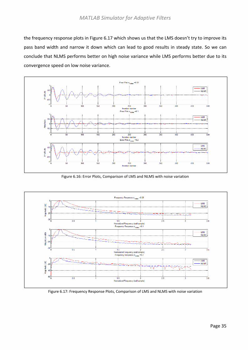
Page 35

the frequency response plots in Figure 6.17 which shows us that the LMS doesn’t try to improve its

pass band width and narrow it down which can lead to good results in steady state. So we can

conclude that NLMS performs better on high noise variance while LMS performs better due to its

convergence speed on low noise variance.

Figure 6.16: Error Plots, Comparison of LMS and NLMS with noise variation

Figure 6.17: Frequency Response Plots, Comparison of LMS and NLMS with noise variation


Page 36

6.2. Stationary Signal with Noise at High Frequencies Only The stationary signal used is a sinusoid signal with frequency, F = 400 Hz and sampled at sampling

frequency, Fs = 12000 and is the desired signal in this case. The noise added to the input signal is

random noise present at frequencies greater than 0.3 π. The noise taken is a normal distributed

data with a mean value of 0 (zero) and a standard deviation of 0.05. The adaptive filter should be

able to make a filter such that it filters out the sinusoidal frequency at angular frequency, f =

0.067π. We expect the filter to be a narrow pass band filter. We will observe the filter and its

behaviour for different cases:

6.2.1. Observing the LMS filter response for different step size

6.2.2. Observing the LMS Filter response for different filter orders

6.2.3. Observing the NLMS Filter response for different step sizes

6.2.4. Observing the NLMS Filter response for different filter orders


6.2.6. Comparing LMS with NLMS for variation in noise

6.2.1. Observing the LMS filter response for different step sizes

In this case the length of the input signal is 500 samples, the stop criterion is set at 0.001, the filter

order at 15, filter type is LMS and three different step sizes used are 0.05 (Red), 0.025 (Blue) and

0.01 (Green). The results are shown below in Figure 6.18, 6.19 and 6.20.

Figure 6.18 shows the plot of estimated output. We can see that lower step size results in a slow

convergence rate. Green line shows that the transient region (region before convergence) is much

greater.

Figure 6.19 shows the error plot, the smaller step size results in the slow convergence rate at the

start but as soon as it enters the steady state we found that smaller step size gives good result by

giving less variation. This shows that the smaller step size approaches steady state late but has a

good response in steady state.


Page 37

Figure 6.18: Estimated Output, Observing the LMS filter response for different step sizes

Figure 6.19: Error Plot, Observing the LMS filter response for different step sizes


Page 38

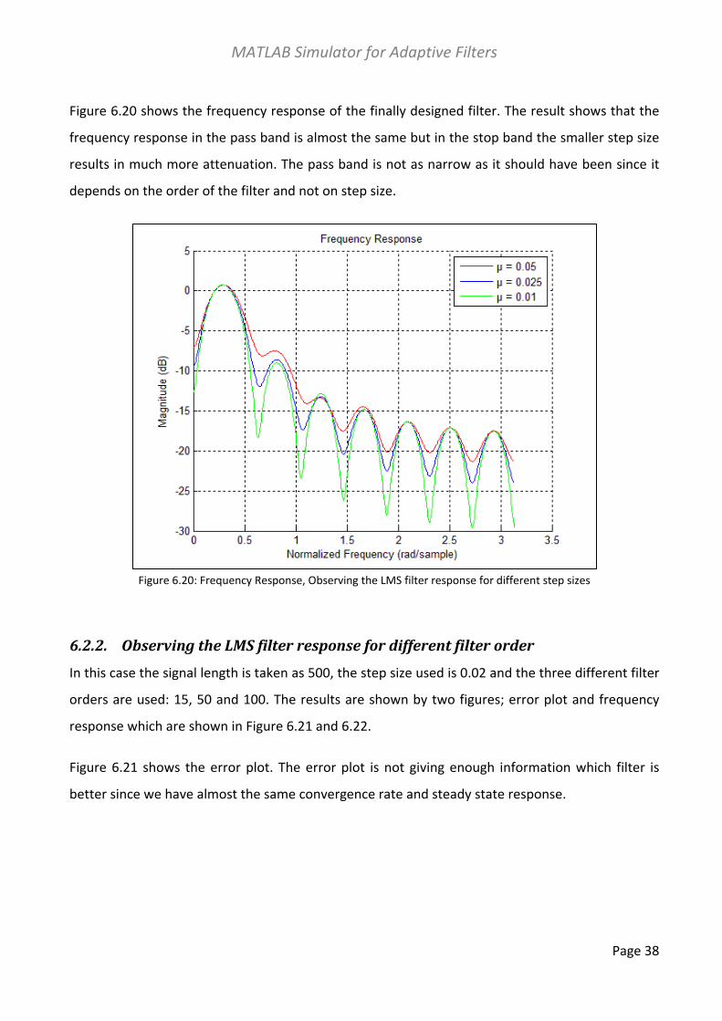
Figure 6.20 shows the frequency response of the finally designed filter. The result shows that the

frequency response in the pass band is almost the same but in the stop band the smaller step size

results in much more attenuation. The pass band is not as narrow as it should have been since it

depends on the order of the filter and not on step size.

Figure 6.20: Frequency Response, Observing the LMS filter response for different step sizes

6.2.2. Observing the LMS filter response for different filter order

In this case the signal length is taken as 500, the step size used is 0.02 and the three different filter

orders are used: 15, 50 and 100. The results are shown by two figures; error plot and frequency

response which are shown in Figure 6.21 and 6.22.

Figure 6.21 shows the error plot. The error plot is not giving enough information which filter is

better since we have almost the same convergence rate and steady state response.


Page 39

Figure 6.21: Error Plot, Observing the NLMS filter response for different step sizes

Figure 6.22: Frequency Response, Observing the NLMS filter response for different step sizes


Page 40

Figure 6.22 which is the frequency response, shows a set of pass band filters and we expected it to

be a narrow pass band filter. We can see that raising the filter order improves the filter response

the response of filter order 50,100 is better than 15 in the pass band and much narrower but is

almost same for both order 50 and 100. Later in the chapter a comparison with NLMS is also done.

6.2.3. Observing the NLMS filter response for different step sizes

The signal length is 500, the filter order is 15 and three different step sizes are used: 0.05, 0.025

and 0.01. The need was to observe the LMS filter under variation of step size to notice the effects.

The results are shown by two figures; error plot and frequency response. The two plots are shown

in Figure 6.23 and 6.24.

Figure 6.23 shows the error plot. The increase in step size results in faster convergence. If we

compare discuss with same scenario LMS which then we will see that overall NLMS takes more

time to converge but the variation is much controlled and less than LMS. Since for NLMS the

convergence time is more but with greater stability we can use higher step sizes for NLMS as

compared to the LMS.


Page 41

Figure 6.23: Error Plot, Observing the LMS filter response for different filter order

Figure 6.24: Frequency Response, Observing the LMS filter response for different step size


Page 42

Figure 6.24 which shows the frequency response indicate that raising step size has no effect of on

the pass band response of the filter. We see better attenuation in stop band for smaller step size

but considering the greater convergence time it takes, the advantage seems to be really less.

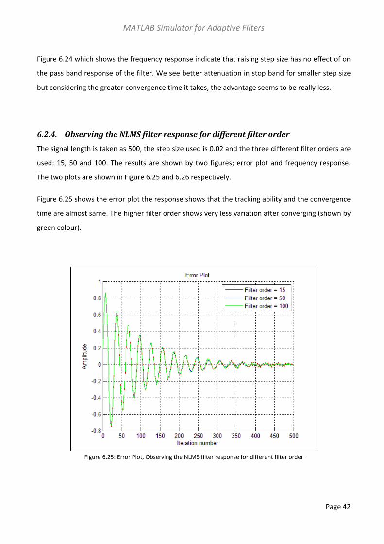
6.2.4. Observing the NLMS filter response for different filter order

The signal length is taken as 500, the step size used is 0.02 and the three different filter orders are

used: 15, 50 and 100. The results are shown by two figures; error plot and frequency response.

The two plots are shown in Figure 6.25 and 6.26 respectively.

Figure 6.25 shows the error plot the response shows that the tracking ability and the convergence

time are almost same. The higher filter order shows very less variation after converging (shown by

green colour).

Figure 6.25: Error Plot, Observing the NLMS filter response for different filter order


Page 43

Figure 6.26: Frequency Response, Observing the NLMS filter response for different filter order

Figure 6.26 which shows the frequency response indicate that raising the filter order improves the

filter response. The filter shows that it is a narrow pass band filter and the expectation was also

the same. The pass band gets much narrower as we raise the filter order. During the same

comparison for LMS in section 6.2.2 we saw the response for filter order 50 and 100. In this case of

NLMS we can clearly see the frequency response of filter order 100 is much better and pass band

is much narrower than filter orders of 50 and 15. The same case compared to LMS shows almost

same frequency response for filter order 50 and 100 but for NLMS it improves.


In this section we will make a comparison between LMS and NLMS for evaluation both under the

same conditions. For this comparison, the signal length is taken as 500, the step size used is 0.025

and the filter order used is 100. The results are shown by four figures; estimated output plot, error

plot, frequency response and learning curve and the four plots are shown in Figure 6.27, 6.28, 6.29

and 6.30 respectively.


Page 44

Figure 6.27: Estimated Output, Comparison of LMS and NLMS

Figure 6.28: Error Plot, Comparison of LMS and NLMS


Page 45

Figure 6.29: Frequency Response, Comparison of LMS and NLMS

Figure 6.27 shows the estimated plot by both LMS and NLMS. We see that NLMS take more time

for estimation than LMS. After estimation both signals look similar, we can see this after 300th

iteration.

Figure 6.28 shows the error plots for both filters. It can be observed in the error plot too that the

convergence rate of NLMS is slower than LMS and performance in steady state is much better. The

frequency response plot of Figure 6.25 shows interestingly that despite the slow speed NLMS

perform much better since the filter by NLMS is much narrower than LMS which is required for

better filtering of the sinusoid.

Figure 6.29 shows us that NLMS filter is much better than LMS filter since the pass band is quite

narrow as per requirement and cutoff of the NLMS filter are quite steep.


Page 46

Figure 6.30: Learning Curve, Comparison of LMS and NLMS

Figure 6.31: Zoomed version of Learning curve, Comparison of LMS and NLMS

Figure 6.30 showed the learning curve, it tells us that the convergence rate of LMS is more than

NLMS but to make sure which one is better in a steady state so we took a zoomed version of

steady state in Figure 6.31 and we can see that NLMS is more stable in steady state.


Page 47


Like previous section 6.1.6., in this section we will also study the impact of noise to the input

signal. The amount of noise in the input signal is changed by changing the variance of noise data.

Variance is the square of standard deviation so we can consider different values of standard

deviation for testing. The three different values of standard deviation of noise data taken are 0.05,

0.1 and 0.2 and the results are shown in Figures 6.32, 6.33, 6.34 and 6.35 respectively.

Figure 6.32 shows a comparison of LMS and NLMS filter for variation in noise. For the LMS filter we

notice that the fluctuation of the error signal in the steady state is higher as the noise standard

deviation increases and the pattern of error is also different from the three noise signals. For the

NLMS it seems like the error signal exactly follow the same pattern for the three noise signals with

rise in value of the signal. This tells us that NLMS behaves the same to the three noises and is good

in the sense that pass band is very narrow.

Figure 6.33 shows the frequency response plot for both filters as we change the noise variance.

The pass band characteristics of both filters, LMS and NLMS, remain almost same. The filter made

by LMS changes mostly in stop band with change in noise variance while that of NLMS almost

remains the same. This shows that NLMS behaviour towards change in noise variance remains

consistent. One possible reason of this can be the normalizing of input signal in case of NLMS. The

noise is present in the input signal and NLMS normalizing that signal, so not effecting the filter

performance.


Page 48

Figure 6.32: Error Plots, Effect of noise variation on LMS and NLMS

Figure 6.33: Frequency Response Plots, Effect of noise variation on LMS and NLMS

If we compare this Figure 6.33 of NLMS with Figure 6.15, the difference was in the input noise. In

this section the noise is not present at low frequency where the desired signal is present but in the

previous section 6.1 noise was present at all frequencies. We can see that when noise is not

present at low frequency the NLMS filter after convergence is almost the same for all cases.


Page 49

Figure 6.34: Error Plots, Comparison of LMS and NLMS with noise variation

Figure 6.35: Frequency Response Plots, Comparison of LMS and NLMS with noise variation

In Figure 6.34 the results indicate one LMS has faster convergence than NLMS. The frequency

response plots in Figure 6.35 which shows us that the LMS doesn’t try to improve its passband

width and narrow it down which can lead to good results in steady state. So we can conclude that

NLMS performs better on high noise variance while LMS performs better due to its convergence

speed on low noise variance.


Page 50

Chapter 7. Result and Analysis of Non-Stationary Signals

In the last chapter the results were discussed adaptive filters applied to stationary signal in detail

along with the effects of step size, filter order and variation of noise signal strength at the input of

the filter. Later we also made a comparison of performance of both filters. Since we know the

effects of step size, filter order and noise variation, so in this chapter when we will cover the result

of filters on non-stationary signals we will consider less cases of step size and filter order. The non-

stationary signals are very special signals and are difficult to handle due to the reason that their

frequency varies with time. For this reason the adaptive filter algorithms find it difficult to track

such signals. We will take a look at the conditions under which the filters work stable and then

make a comparison between the two filters.

7.1. Non-Stationary Signal with Sinousidal Noise The non-stationary signal used for testing is a speech signal sampled at Fs = 22.5 kHz. The first case

of noise is a sinusoid added at a frequency, f = 0.66π. This makes the input signal to be a speech

signal plus sinusoidal noise. The expectation form filter will be that it creates a notch filter so that

it filter out the sinusoid from the input signal.

7.1.1. Results of LMS filter

We chose a step size value, µ = 0.02 and filter order = 200 in this case. The filter order is kept a

little higher than the cases of a stationary signal because we need to minimize the width of

stopband of the notch filter. The results are shown in Figure 7.1, 7.2 and 7.3.

Figure 7.1 shows the output of the filter along with the original signal i.e. speech signal. While

looking at it we can see that both the figures are close enough so that output is close match of the

desired signal. The exact amount of difference between the two signals can be seen in the error

plot.


Page 51

Figure 7.1: Estimated and Desired signal for LMS, µ = 0.02

Figure 7.2: Error plot for LMS, µ = 0.02


Page 52

Figure 7.2 shows the error plot which tells us that the estimated signal is much close to desire but

there are some small peaks in the transient. One obvious reason for this can the nature of the

signal we are dealing with i.e. the stationary signal, since the signal frequency changes so it was

expected up to some extent.

Figure 7.3 which is the frequency response shows good result. It makes a good notch filter at the

frequency where the sinusoidal noise exists. Problems lie in the passband where we see an

undesirable dip of -1 dB.

Figure 7.3: Frequency response for LMS, µ = 0.02

We tried to improve LMS performance in this case by increasing our parameter step size which we

know from previous section increasing the tracking ability of the filter. We face another problem

that if we raise the step size a little more than the filter becomes unstable. See Figure 7.4

(Frequency Response plot) and Figure 7.5 (Error plot) showing that the filter gets unstable when

the step size is raised from 0.02 to 0.07.


Page 53

Figure 7.4: Frequency response for LMS, µ = 0.07

Figure 7.5: Error plot for LMS, µ = 0.07


Page 54

7.1.2. Results of NLMS filter

For the NLMS filter we have taken step size, µ = 0.02 and filter order = 200. Again the filter order is

kept a little higher than the previous chapter. The results are shown in Figure 7.6, 7.7 and 7.8.

Figure 7.6 shows the output of filter i.e. estimated output signal along with the original signal.

While looking at it we can see that both the figures are close enough. The exact amount of

difference between the two signals can be seen in the error plot.

Figure 7.7 shows the error plot which tells us that the estimated signal is much close to desire but

there are some small peaks in the transient which are mainly due to frequency changing nature of

the signal but other factors can be seen after taking a look at the frequency response of the finally

designed filter.

Figure 7.6: Estimated and desired signals plot for NLMS, µ = 0.02


Page 55

Figure 7.7: Error plot for NLMS, µ = 0.02

Figure 7.8: Frequency Response plot for NLMS, µ = 0.02


Page 56

Figure 7.8 which is the frequency response shows good result. It makes a good notch filter at the

frequency where the sinusoidal noise exists but for the pass band we again see some small dips at

low frequencies. We again test by increasing our step size.

The step size is considered a little high so that we can catch up with the signal during the run of

the algorithm. Unlike LMS, NLMS filter doesn’t become unstable when increased from 0.02 to 0.07

but it enhanced the performance. The normalizing ability of NLMS prevented it from getting

unstable. The stability of NLMS and high convergence rate of high step size results in an overall

better performance. See Figure 7.9 and 7.10.

Figure 7.9 is the error plot for NLMS at step size=0.07 and it shows us that the error is now very

less than what we saw in Figure 7.7 when step size was 0.02. This tells us that the estimated signal

is quite close to the desired signal.

Figure 7.9: Error plot for NLMS, µ = 0.07

If we see Figure 7.10 showing the frequency response of the NLMS filter at step size we see that

now have got a really good notch filter which filters out the undesirable sinusoid from the speech

signal.


Page 57

Figure 7.10: Frequency Response plot for NLMS, µ = 0.07

Considering above results we can conclude two things. One NLMS works for sure better than LMS

in the above tested case. Secondly NLMS has really less chances getting unstable compared to LMS

which gives it the edge to increase the step size where tracking ability enhancement is required.

7.2. Non-Stationary Signal With Random Noise Moving from a simple noise case to an advance case for testing we have for this section a random

noise present at frequencies greater than 0.5 Fs. The noise taken is a normal distributed data with

a mean value of 0 (zero) and a standard deviation of 0.005. The non-stationary signal used is a

speech signal sampled at Fs = 22.5 kHz. The expectation form filter will be that it creates a kind of

low pass filter with cutoff around 0.5 Fs so that is filtered out noise from the speech signal.

7.2.1. Results of LMS filter The parameters for the LMS filter we have taken are step size, µ = 0.02 and filter order = 200. The

results are shown in Figures 7.11, 7.12 and 7.13.


Page 58


Figure 7.12: Error Plot for LMS, µ = 0.02


Page 59

Figure 7.11 shows the output of the filter along with the original signal i.e. speech signal. Both

figures are close enough but again the exact extent of matching can be seen through the error

plot.

Figure 7.12 showing the error plot with step size µ = 0.02 tells us that the variation of error signal

in the steady state is quite high. The small peaks are less but the random noise has played its role

in keeping the error high even in the steady state.

In Figure 7.12 there is a lot of variation in the error signal from the start than even after achieving

steady state there are some small peaks but the error exists at large. This shows us the LMS

doesn’t show good results for non-stationary signal (which is speech signal) with random noise

addition.

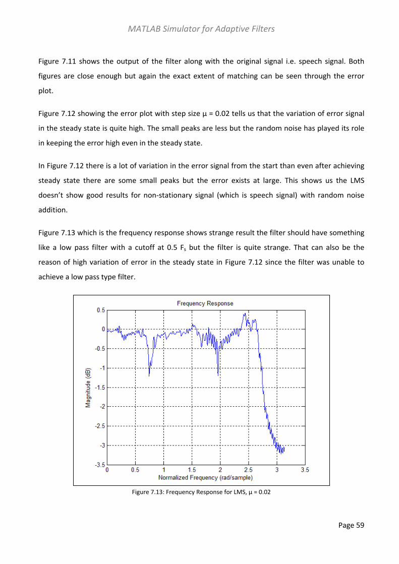
Figure 7.13 which is the frequency response shows strange result the filter should have something

like a low pass filter with a cutoff at 0.5 Fs but the filter is quite strange. That can also be the

reason of high variation of error in the steady state in Figure 7.12 since the filter was unable to

achieve a low pass type filter.

Figure 7.13: Frequency Response for LMS, µ = 0.02


Page 60

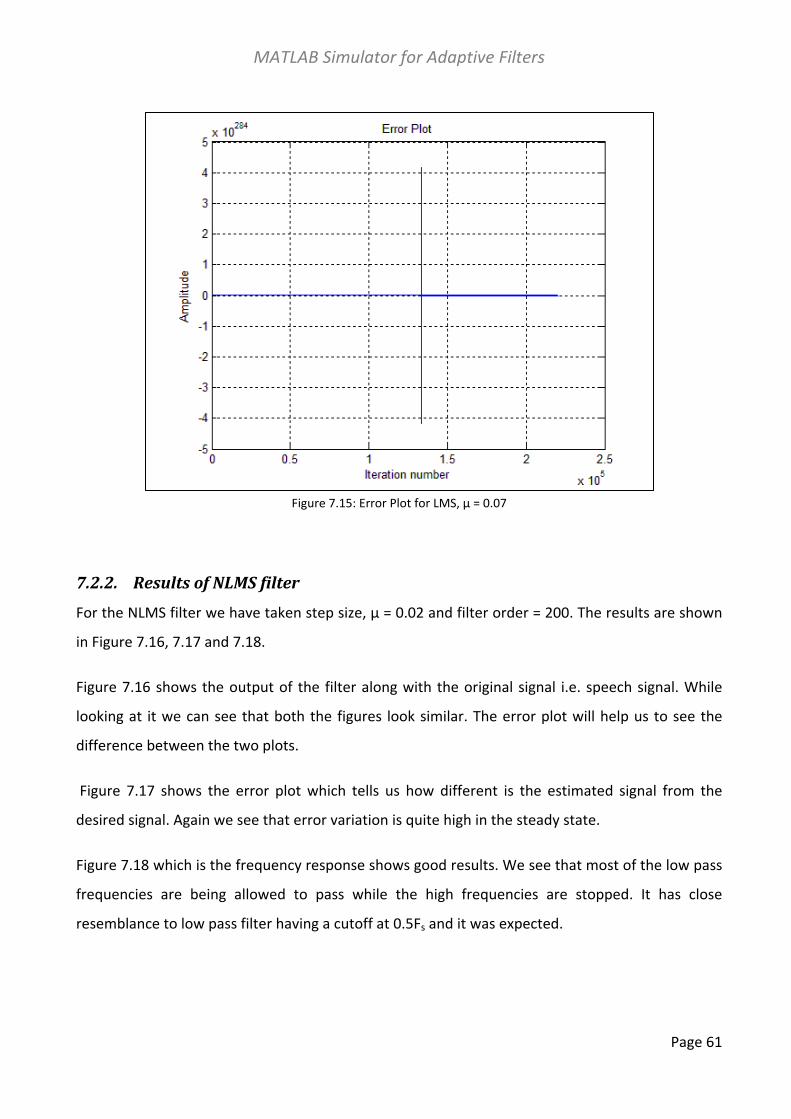
Then we raised the step size to improve the filter’s tracking ability but we achieved instability of

LMS. See Figure 7.14 (Frequency Response Plot) and 7.15 (Error Plot) showing that the filter gets

unstable when the step size is raised from 0.02 to 0.07. The values of the filter’s frequency

response indicate how unstable LMS went when its step size was increased.



Page 61

Figure 7.15: Error Plot for LMS, µ = 0.07

7.2.2. Results of NLMS filter For the NLMS filter we have taken step size, µ = 0.02 and filter order = 200. The results are shown

in Figure 7.16, 7.17 and 7.18.

Figure 7.16 shows the output of the filter along with the original signal i.e. speech signal. While

looking at it we can see that both the figures look similar. The error plot will help us to see the

difference between the two plots.

Figure 7.17 shows the error plot which tells us how different is the estimated signal from the

desired signal. Again we see that error variation is quite high in the steady state.

Figure 7.18 which is the frequency response shows good results. We see that most of the low pass

frequencies are being allowed to pass while the high frequencies are stopped. It has close

resemblance to low pass filter having a cutoff at 0.5Fs and it was expected.


Page 62

Figure 7.16: Estimated and Desired signal for NLMS, µ = 0.02

Figure 7.17: Error Plot for NLMS, µ = 0.02


Page 63

Figure 7.18: Frequency Response for NLMS, µ = 0.02

Figure 7.19: Frequency Response for NLMS, µ = 0.07


Page 64

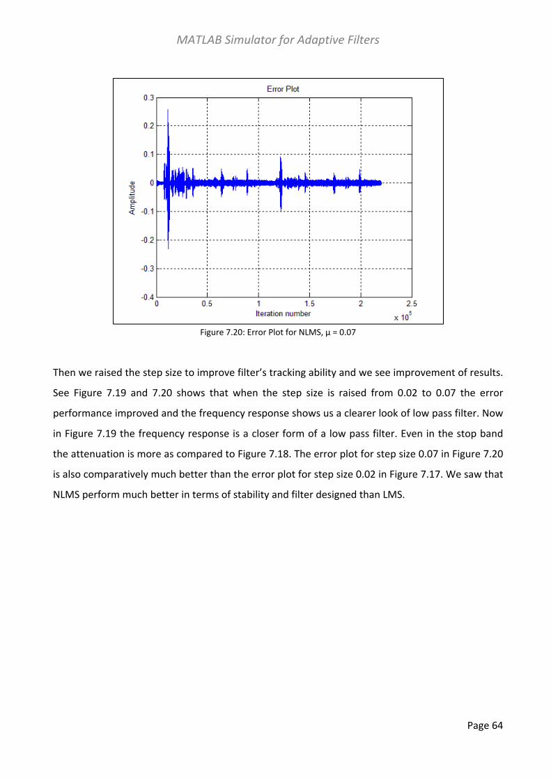
Figure 7.20: Error Plot for NLMS, µ = 0.07

Then we raised the step size to improve filter’s tracking ability and we see improvement of results.

See Figure 7.19 and 7.20 shows that when the step size is raised from 0.02 to 0.07 the error

performance improved and the frequency response shows us a clearer look of low pass filter. Now

in Figure 7.19 the frequency response is a closer form of a low pass filter. Even in the stop band

the attenuation is more as compared to Figure 7.18. The error plot for step size 0.07 in Figure 7.20

is also comparatively much better than the error plot for step size 0.02 in Figure 7.17. We saw that

NLMS perform much better in terms of stability and filter designed than LMS.


Page 65

Chapter 8. Conclusion

In chapter 6 we covered the effects of stationary signals on the performance of adaptive filters.

The two adaptive filters used were LMS and NLMS. Two types of test signals were used, one was

random noise present on all frequencies in section 6.1 and another was random noise present of

high frequencies only. Noise was added to the signal to create the input signal to the adaptive

filters. The system was required to cancel the effect of noise to estimate the desired signal. We

created different scenarios to see the effects. We tested the signal with variation in step size, filter

order and noise variance. The effects of changes in parameters were noted within a specific filter

and later a comparison between the filters was done.

The first test led us to conclude the step size increases the convergence speed of a filter from

transient to steady state but at the same time increase the error variation in the steady state. This

trade-off between the convergence speed and error variation can be set with the help of a

suitable step size depending upon signal requirement.

The second test on the filter order helped us to see how the filter frequency response varies with

variation in filter order. The filter order can be set according to the expectation of the final filter. If

the requirement of the filter’s cutoff is steeper than it should be kept high at the cost of

computation time and gain of less noise at the output through the pass band but if the error

minimization requirement is less strict we are allowed to the keep the filter order low.

The testing of variation in noise helped us to understand how the adaptive filter algorithm

behaves with the increase in noise variance. NLMS seemed to behave consistent with variation in

noise as we inspected the filter’s frequency response. This was also due to the normalization

action done on the input signal containing the noise by the NLMS filter. LMS showed changes in

filter’s frequency response with variation in noise.

Also we came to know the NLMS due to normalization of input slowly converges to a steady state

while LMS is faster in convergence. LMS showed more variation in steady state and good


Page 66

frequency response even with low filter order while LMS need high filter order to attain similar

results. NLMS also showed consistency to changes in noise variance.

In chapter 7 we covered the effects of non-stationary signals whose frequency is varying with

time. NLMS performs much better the LMS for the non-stationary signal that is much more

difficult to handle. The performance can be accessed from multiple parameters. Some of the

reasons were same that are discussed in conclusive remarks from chapter 6 from above. The

estimated output by NLMS were closer to the desired signal as compared to the LMS when we

evaluated the error plots. If we consider stability we saw that NLMS was very stable because LMS

became unstable at higher step size. NLMS escaped from instability due to its normalizing nature.

Considering filter design we saw NLMS was more targeted and close to the expected filter.

The amount of variation in non-stationary signal is difficult to control. LMS has relatively poor

performance for non-stationary as compared to NLMS. LMS performs well for signals with prior

knowledge that is why the results of LMS for non-stationary signals are not satisfactory. On the

other hand NLMS allow stable performance for non-stationary signals. The slow convergence rate

of NLMS can be controlled by increasing step size but in limited amounts. Considering the amount

of stability and good performance we can clearly say that NLMS is much better than LMS for Non-

stationary signals.

If consider the computational cost of LMS and NLMS at same parameter and we take a look at the

number of multiplications we found out that the number of multiplications for the LMS are 2N+1

and for NLMS are 3N+1, so the NLMS is expensive in computation.

Now for future work there is a lot of scope to work on adaptive filters. The filters made by LMS

and NLMS are FIR filters and we have some adaptive filter like FxLMS that uses IIR filter so a

comparison between them will be good.

Step size plays an important role but due to its constant nature during algorithm execution the

trade-off becomes important. A lot of work in the field of adaptive step size is done to improve

filter performance. This is another important dimension in which further work or comparison of

proposed techniques for adaptation can be done.


Page 67

References

[1] ACOUSTIC ECHOCANCELLATION USING DIGITALSIGNAL PROCESSING, By Michael Hutson

The School of Information Technology and Electrical Engineering, The University of Queensland.

[2] Diniz, Paulo S. R. 1997, Adaptive Filtering, Algorithms and Practical Implementation. Kluwer

Academic Publishers, Boston.

[3] Haykin, Simon. 1991, Adaptive Filter Theory.2nd Edition. Prentice-Hall Inc., New Jersey.

[4] Farhang-Boroujeny, B. 1999, Adaptive Filters, Theory and Applications. John Wiley and Sons,

New York.

[5] Oppenheim, Alan V., Schafer, Ronald W. 1989, Discrete-Time Signal Processing, International

edition. Prentice-Hall, Inc., New Jersey.

atlab simulator for adaptive filters - diva portal829400/fulltext01.pdfmatlab simulator for adaptive...

Documents