tsz ping (charley) chan b.s.e.e. (with highest distinction
TRANSCRIPT

REITERATIVE MINIMUM MEAN SQUARE ERROR ESTIMATOR
FOR DIRECTION OF ARRIVAL ESTIMATION
AND BIOMEDICAL FUNCTIONAL BRAIN IMAGING
BY
Tsz Ping (Charley) Chan
B.S.E.E. (With Highest Distinction), University of Kansas, 2006
Submitted to the Department of Electrical Engineering and Computer Science and the Faculty of the Graduate School of the University of Kansas in partial fulfillment of the requirements for the degree of Master of Science.
Thesis Committee:
Dr. Shannon Blunt, Chair
Dr. James Stiles, Committee Member Dr. Arvin Agah, Committee Member Dr. Mihai Popescu, Committee Member
Date Defended: July 18, 2008

I
The thesis committee for Tsz Ping Chan certifies
that this is the approved version of the following thesis:
Reiterative Minimum Mean Square Error Estimator
for Direction of Arrival Estimation
and Biomedical Functional Brain Imaging
Thesis Committee:
Dr. Shannon Blunt, Chair
Dr. James Stiles, Committee Member Dr. Arvin Agah, Committee Member Dr. Mihai Popescu, Committee Member
Date Approved: July 18, 2008

II
ACKNOWLEDGEMENTS
First of all, I would like to thank my advisor, Dr. Shannon Blunt, for his
invaluable guidance, financial support, friendship and patience throughout the past
two years. Not only did he provide insightful advice pertaining to academics and
research, he also shared with his advisee his life experience to which I can closely
relate. I am also grateful for the opportunities he opened up for me during my
graduate career, especially the chance to work on bioengineering-related research. I
will always remember to trust my own intuition as advised by Dr. Blunt.
I would also like to thank Dr. Mihai Popescu for familiarizing me with the
background knowledge required for the neuroimaging research and also for involving
me in his research projects. Additionally, I would like to thank Dr. Jim Stiles and
Dr. David Petr for making the most difficult subjects fun and more intuitive to learn
and for being very patient and helpful to students. I would also like to thank Dr. Agah
for his humor and his kind help of serving on my committee.
I would like to thank my first research mentor, John Paden, for initiating my
interest in signals processing and mathematics, taking on the not-so-pleasant tasks of
training a new researcher, and demonstrating diligence in the research he loved. I owe
thanks to my co-worker and classmate, Tommy Higgins, for his friendship, the
enormous amount of encouragement, meaningful advices, and being the one who
constantly challenges my ideas. Noah Watkins and Terry Lau also deserve my thanks
for their friendship and emotional support in the past years.
Most importantly, I would like to thank my parents for their unconditional
love, the lessons they taught me to equip me to fulfill my dreams and the sacrifices
they made to make my education in America possible.

III
ABSTRACT
Two novel approaches are developed for direction-of-arrival (DOA)
estimation and functional brain imaging estimation, which are denoted as ReIterative
Super-Resolution (RISR) and Source AFFine Image REconstruction (SAFFIRE),
respectively. Both recursive approaches are based on a minimum mean-square error
(MMSE) framework.
The RISR estimator recursively determines an optimal filter bank by updating
an estimate of the spatial power distribution at each successive stage. Unlike previous
non-parametric covariance-based approaches, which require numerous time
snapshots of data, RISR is a parametric approach thus enabling operation on as few
as one time snapshot, thereby yielding very high temporal resolution and robustness
to the deleterious effects of temporal correlation. RISR has been found to resolve
distinct spatial sources several times better than that afforded by the nominal array
resolution even under conditions of temporally correlated sources and spatially
colored noise.
The SAFFIRE algorithm localizes the underlying neural activity in the brain
based on the response of a patient under sensory stimuli, such as an auditory tone.
The estimator processes electroencephalography (EEG) or magnetoencephalography
(MEG) data simulated for sensors outside the patient's head in a recursive manner
converging closer to the true solution at each consecutive stage. The algorithm
requires a minimal number of time samples to localize active neural sources, thereby
enabling the observation of the neural activity as it progresses over time. SAFFIRE
has been applied to simulated MEG data and has shown to achieve unprecedented
spatial and temporal resolution. The estimation approach has also demonstrated the
capability to precisely isolate the primary and secondary auditory cortex responses, a
challenging problem in the brain MEG imaging community.

IV
TABLE OF CONTENTS
ACKNOWLEDGEMENTS ................................................................................................................. II ABSTRACT ......................................................................................................................................... III TABLE OF CONTENTS .................................................................................................................... IV TABLE OF FIGURES ........................................................................................................................ VI TABLE OF TABLES .......................................................................................................................... IX CHAPTER 1: INTRODUCTION ........................................................................................................ 1
1.1 OVERVIEW ..................................................................................................................................... 1 1.2 DIRECTION OF ARRIVAL ESTIMATION ........................................................................................... 1 1.3 NEURAL SOURCE LOCALIZATION .................................................................................................. 2 1.4 THESIS OUTLINE ............................................................................................................................ 4
CHAPTER 2: BACKGROUND ........................................................................................................... 6 2.1 DIRECTION OF ARRIVAL ESTIMATION ........................................................................................... 6
2.1.1 Physical Scenario and Signal Representation ...................................................................... 6 2.1.2 Signal Correlation and Spectral Super Resolution ............................................................... 9
2.2 NEURAL SOURCE LOCALIZATION ................................................................................................ 10 2.2.1 Neural Mechanism and Imaging Techniques ...................................................................... 10 2.2.2 The Leadfield Matrix .......................................................................................................... 14 2.2.3 Forward Signal Model and The Inverse Problem ............................................................... 18
2.3 FILTER THEORY ........................................................................................................................... 19 2.3.1 Matched Filter .................................................................................................................... 19 2.3.2 MUltiple SIgnal Classification (MUSIC) ............................................................................ 21 2.3.3 Minimum Mean Square Error Estimators .......................................................................... 24 2.3.4 FOCal Underdetermined System Solution .......................................................................... 27 2.3.5 Discussion of Direction of Arrival Algorithms ................................................................... 29 2.3.6 Discussion of Neural Localization Algorithms ................................................................... 30
CHAPTER 3: RE-ITERATIVE SUPER-RESOLUTION ............................................................... 32 3.1 REITERATIVE MINIMUM MEAN SQUARE ERROR ESTIMATOR ...................................................... 32 3.2 RISR ALGORITHM ....................................................................................................................... 35 3.3 SPECTRAL OVER-SAMPLING ........................................................................................................ 37 3.4 MULTIPLE-TIME PROCESSING...................................................................................................... 38
3.4.1 Incoherent Integration ........................................................................................................ 39 3.4.2 Eigen Decomposition .......................................................................................................... 41 3.4.3 Additional Methods ............................................................................................................. 42
CHAPTER 4: SOURCE AFFINE IMAGE RECONSTRUCTION ................................................ 44 4.1 SAFFIRE ALGORITHM ................................................................................................................ 44
4.1.1 Basic Algorithm .................................................................................................................. 44 4.1.2 AFFINE TRANSFORMATION OF SOLUTION SPACE .................................................... 45 4.1.3 Matched Filter Bank Initialization ...................................................................................... 46 4.1.4 Energy Normalization ......................................................................................................... 48 4.1.5 Noise Covariance Estimation ............................................................................................. 51 4.1.6 Implementation ................................................................................................................... 51

V
4.1.7 Reconstruction of Dipole Time Course ............................................................................... 52 4.2 MULTIPLE-TIME PROCESSING...................................................................................................... 53 4.3 MULTIPLE-STAGES FOR VOLUMETRIC CONSTRAINTS .................................................................. 55
CHAPTER 5: SIMULATION RESULTS AND DISCUSSION ...................................................... 56 5.1 RISR ........................................................................................................................................... 56
5.1.1 Performance Metrics .......................................................................................................... 56 5.1.2 Basic Performance .............................................................................................................. 57 5.1.3 Temporal Robustness .......................................................................................................... 63 5.1.4 Spectral Super-Resolution .................................................................................................. 67 5.1.5 Data Sample Support .......................................................................................................... 69 5.1.6 Calibration Error ................................................................................................................ 71 5.1.7 Colored Additive Noise ....................................................................................................... 73 5.1.8 Observation of Sparse Solution Convergence ..................................................................... 75
5.2 SAFFIRE .................................................................................................................................... 76 5.2.1 Experimental Setup and MEG Configurations ................................................................... 76 5.2.2 Single Dipole Activation ..................................................................................................... 78 5.2.3 Nearby Dipole Pair ............................................................................................................. 89 5.2.4 Mirrored Dipole-Pair in Primary Auditory Regions .......................................................... 91 5.2.5 Auditory Response .............................................................................................................. 92 5.2.6 Time-Course Reconstruction with Interference .................................................................100
CHAPTER 6: CONCLUSIONS AND FUTURE WORK ...............................................................104 6.1 CONCLUSIONS ............................................................................................................................104 6.2 FUTURE WORK ...........................................................................................................................105

VI
TABLE OF FIGURES
Figure 2-1. Physical setup of M = 1 source signal impringing on an ULA of N sensors................................................................................................................... 7
Figure 2-2. Structural composition of a neuron [19] ................................................... 11 Figure 2-3. Biomagnetometer system with 151 channels during cortical MEG
recording at the Hoglund Brain Imaging Center in KUMC ............................... 12 Figure 2-4. Magnetic field B of a current I ................................................................ 13 Figure 2-5. Sorted leadfield vector norms for dipoles in the brain sample space ...... 17 Figure 2-6. Eigen spectrum of the auto-correlation matrix of leadfield matrix B ..... 17 Figure 2-7. Normalized inner-product of steering vectors ......................................... 20 Figure 2-8. Block diagram of statistical filtering for estimation ................................ 24 Figure 3-1. Block diagram of the RISR operation ...................................................... 36 Figure 3-2. Block diagram of I2-RISR operation ....................................................... 40 Figure 5-1. Angular spectrum (in electrical degrees) of RISR with K = 1 snapshot,
N = 10, SNR = 35 dB and uncorrelated sources over the first 8 iterations ....... 58 Figure 5-2. Angular spectrums of different algorithms with uncorrelated sources at
-90°, -72° and 0°, K = 20 samples, SNR = 20 dB ............................................... 59 Figure 5-3. Probability of separation of RISR, e-RISR and RISR with C as input
versus SNR for uncorrelated sources, K = 20 samples ...................................... 60 Figure 5-4. Angular root mean square error of RISR, e-RISR and RISR with C as
input versus SNR for uncorrelated sources, K = 20 samples ............................. 61 Figure 5-5. Probability of separation of RISR, MUSIC and SS-MUSIC versus SNR for
uncorrelated sources, K = 20 samples ............................................................... 62 Figure 5-6. Angular root mean square error of RISR, MUSIC and SS-MUSIC versus
SNR for uncorrelated sources, K = 20 samples .................................................. 63 Figure 5-7. Anecdotal results of RISR, MUSIC and SSMUSIC with sources at -90°,
-72° (correlated with source at -90°) and 0°, K = 20 samples, SNR = 35 dB .... 64 Figure 5-8. Probability of separation of RISR, MUSIC and SS-MUSIC versus SNR for
correlated sources at -90°, -81° and an uncorrelated at 0°, K = 20 samples .... 65 Figure 5-9. Angular root mean square error of RISR, MUSIC and SS-MUSIC versus
SNR for correlated source, K = 20 samples ....................................................... 66 Figure 5-10. Monte Carlo simulation result of POS for two uncorrelated signals over
a range of super-resolution factor L versus SNR for RISR and SS-MUSIC algorithms ........................................................................................................... 67
Figure 5-11. Monte Carlo simulation result of ARMSE for two uncorrelated signals over a range of super-resolution factor L versus SNR for RISR and SS-MUSIC algorithms ........................................................................................................... 68
Figure 5-12. Probability of separation of RISR versus SNR for uncorrelated sources at -90°, -81° and 0° and K = 1, 2, 4, 8, 16 and 500 snapshots ........................... 69
Figure 5-13. Probability of separation of SS-MUSIC versus SNR for uncorrelated sources at -90°, -81° and 0° and K = 1, 2, 4, 8, 16 and 500 snapshots .............. 70

VII
Figure 5-14. Effect of calibration error on RISR and SS-MUSIC at each antenna element for three uncorrelated sources for amplitude error of 5% and phase error of 5% .......................................................................................................... 71
Figure 5-15. Probability of separation versus percentage calibration error in amplitude and in phase for RISR and SS-MUSIC with three uncorrelated sources at SNR = 25 dB and K = 40 snapshots ............................................................... 73
Figure 5-16. Angular spectrum of estimated signal strengths for different algorithms with 3 uncorrelated signals and addictive noise with mainlobe at around 45º .. 74
Figure 5-17. Ten most dominant eigen values of matrix P at the 15th iteration for the estimation of (a) a single signal source at -90°; (b) two uncorrelated signals at -90° and -45°; (c) three uncorrelated signals at -90°, -45° and 0° ................... 76
Figure 5-18. Physical configuration of 150 MEG sensors relative to the brain ........ 77 Figure 5-19. Activation curve for single dipole activation ......................................... 78 Figure 5-20. Mean Global Field Power and the sensors response of the simulated
MEG measurements corresponding to single dipole activation. ........................ 79 Figure 5-21. The angled and front/top view of the location of the true active dipole
8981, which is 6.1 cm from the center of the brain, estimated by (a) SAFFIRE using K = 1 snapshots; (b) SAFFIRE using K = 4 snapshots; (c) FOCUSS e; and (d) MNE with a threshold of 70% of maximum estimated dipole strength ......... 81
Figure 5-22. Dipole strength estimated by SAFFIRE, the neural activity index resulted from LCMV algorithm, and the dipole strength estimated by MNE for activated dipole 8981 .......................................................................................... 82
Figure 5-23. True activation curve of dipole 8981 and reconstructed time course of dipole activity by (a) SAFFIRE algorithm with K = 4 snapshots and (b) LCMV with 400 snapshots to construct the data covariance matrix .............................. 83
Figure 5-24. The angled and front/top view of the location of the true active dipole 7952, which is 4.4 cm from the center of the brain, estimated by (a) SAFFIRE using K = 1 snapshots; (b) SAFFIRE with K = 4 snapshots; and (c) FOCUSS 85
Figure 5-25. True activation curve of dipole 7952 and reconstructed time course of dipole activity by (a) SAFFIRE algorithm with K = 4 snapshots and (b) LCMV with 400 snapshots to construct the data covariance matrix .............................. 86
Figure 5-26. The angled and front/top view of the location of the true active dipole 3310, which is 2.0 cm from the center of the brain,............................................ 87
Figure 5-27. Dipole strength estimated by SAFFIRE on the left and the neural activity index resulted from LCMV algorithm on the right for activated dipole 3310 .... 88
Figure 5-28. True activation curve of dipole 3310 and reconstructed time course of dipole activity by (a) SAFFIRE algorithm with K = 4 snapshots and (b) LCMV with 400 snapshots to construct the data covariance matrix .............................. 88
Figure 5-29. Dipole strength estimated by SAFFIRE and the neural activity index resulted from LCMV algorithm for the dipole pair 8570 and 8629 ................... 89
Figure 5-30. Angled and front 3D-view of dipoles 8570 and 8629, which are 1.09 cm apart and about 5 cm from the center of the brain, and dipole estimated by SAFFIRE using K = 4 snapshots ....................................................................... 90

VIII
Figure 5-31. Reconstructed time course of dipole 8570 and 8629 using SAFFIRE and the true dipole activation curve .......................................................................... 90
Figure 5-32. Angled and front 3D-view of the dipoles in the primary auditory regions and dipole estimated by SAFFIRE using K = 4 snapshots ................................. 91
Figure 5-33. Reconstructed time course of dipole 1088 and 7952 in the auditory region using SAFFIRE and the true dipole activation curve .............................. 92
Figure 5-34. Locations of the dipole pairs in primary cortex and secondary cortex for the ASSR simulation ............................................................................................ 93
Figure 5-35. Activation curves of primary and secondary auditory regions with peaks at t = 1 and 1.05 s, the mean global field power of the received signals (top right) and the MEG sensors response of all 150 channels ................................. 94
Figure 5-36. An example of the first stage. Top: true dipoles responsible for ASSR and the dipole locations estimated by SAFFIRE-2 with 3-of-5 detector in 3D plot for data at around t = 972 ms (584th sample); bottom: MGFP plot from t = 968 ms to t = 1.085 with primary and secondary activation curves which are out of scale. The black vertical line indicates t = 972 ms on the time axis................... 97
Figure 5-37. An example of the second stage. Top: true dipoles responsible for ASSR and the dipole locations estimated by SAFFIRE-2 with 3-of-5 detector in 3D plot for data at around t = 1.025s (616th sample); bottom: MGFP plot from t = 968 ms to t = 1.085 with primary and secondary activation curves which are out of scale. The black vertical line indicates t = 1.025 s on the time axis .................. 98
Figure 5-38. An example of the third stage. Top: true dipoles responsible for ASSR and the dipole locations estimated by SAFFIRE-2 with 3-of-5 detector in 3D plot for data at around t = 1.052s (632rd sample); bottom: MGFP plot from t = 968 ms to t = 1.085 with primary and secondary activation curves which are out of scale. The black vertical line indicates t = 1.052 s on the time axis .............. 99
Figure 5-39. Activation curves of dipoles 1088 and 7952 in the primary cortex with peak delay of 500 ms and the MGFP plot of the MEG sensor signal ............... 101
Figure 5-40 Angled and front 3D-view of dipoles 1088 and 7952 in the primary cortex with 500 ms peak delay and the dipole estimated by SAFFIRE. The bottom plot is the reconstructed time course of the .......................................... 101
Figure 5-41. Angled and front 3D-view of dipoles 1088 and 7952 in the primary cortex with 500 ms peak delay and the dipoles estimated by SAFFIRE. The bottom plots are the reconstructed time course of the dipoles 1088 and 7952 and the true activation curve ............................................................................ 102

IX
TABLE OF TABLES
Table 3-1. RISR and MMSE variables ........................................................................ 32 Table 5-1. Ideal time indices for first to third stages of ASSR estimation. The bracket
value is the sample index corresponding to the time .......................................... 96 Table 5-2. Estimated time of ASSR dipole localization for the three processing
schemes ............................................................................................................... 96

1
CHAPTER 1: INTRODUCTION
1.1 Overview
Numerous filter techniques have been developed over the past few decades to
solve a branch of problems consisting of a sensor array receiving signals from single
or multiple sources transmitted through some medium. The goal of these techniques
is to localize the signal source in either two or three dimensions by applying an
adaptive filter to the signal received at the sensor array. The direction of arrival
estimation problem addressed in this thesis falls directly under this category.
Although the neural signal reconstruction problem addressed in the rest of this thesis
comes from a very different area of signal processing application, it belongs to the
aforementioned branch of problems because of the signal modeling of the system.
The proposed solutions to the direction of arrival estimation and to the neural signal
reconstruction were formulated based on the same mathematical framework, which
was inspired from a radar adaptive pulse compression processing technique. Due to
the degradation of most existing DOA estimation methods under correlated signals,
the robustness to source correlation contributes to one of the most important
advantages of the proposed approach. These two algorithms also achieve high spatial
resolution compared to other approaches for the respective problems. Other
applications of this general estimator framework include radar signal processing [1],
telecommunications [2], etc.
The introduction and motivation for each of the two algorithms is discussed
in the next two subsections.
1.2 DIRECTION OF ARRIVAL ESTIMATION
Direction of arrival (DOA) estimation has been an area of active research in
the past decades with strong focuses on the applications in communications, radar
and medical imaging [3]. The physical scenario for the estimation problem consists

2
of narrowband radio frequency (RF) signals, which are transmitted by sources in the
far field, impringing in the form of planewaves upon some sensors in a particular
spatial arrangement. A common type of sensor configuration is the uniform linear
array (ULA) antenna [4, 5], which is composed of equally spaced sensor elements.
With the planewave assumption, the received signal at a sensor can be
mathematically expressed as the summation of signal energy from all directions in
space with phase delays across sensor elements.
Matched filtering, i.e. the conventional beamformer [4], and Multiple SIgnal
Classification (MUSIC) [6, 7] are among the more commonly used signal processing
approaches for this problem. However, the low resolution of matched filtering and
the signal correlation intolerance of MUSIC are drawbacks that lead to further
research on DOA estimation techniques. Some filtering methods such as spatially-
smoothed MUSIC (SS-MUSIC) [8] and the Least-Squares-based FOCal
Underdetermined System Solver (FOCUSS) [9,10] are developed to fix the
drawbacks of the previous approaches yet with the cost of lower spectral resolution,
increased amount of prior knowledge, filter regularization, etc. These methods will
be introduced in more details in the Chapter 2. Inspired by the work done for a radar
adaptive pulse compression (APC) algorithm [1], the approach proposed in this
study, denoted as Re-Iterative Super-Resolution (RISR), is a parametric estimator
that iteratively estimates the spectral power by adaptively updating the filter bank at
each stage without the need of prior knowledge. RISR tolerates correlated signals as
well as colored noise, while also achieves angular super-resolution. This approach
will be thoroughly discussed throughout Chapter 3.
1.3 NEURAL SOURCE LOCALIZATION
Electroencephalography (EEG) and magnetoencephalography (MEG) are
imaging techniques used in clinical and research settings to measure the electrical
and magnetic fields generated directly by the electrical activity of the brain. The main
clinical application of MEG is functional brain imaging in which it allows

3
non-invasive detection of neural activities, ensuring the safety of the patient. Brain
imaging involves estimating the locations of brain activity based on the recordings of
sensor elements surrounding the head. In essence, this localization problem is the
extension of the direction of arrival estimation in which the location of a region of
brain activity is estimated. Signal processing techniques are developed to determine
the precise spatial location of underlying active neural sources [4]. It is done by
processing measurements obtained by an array of MEG/EEG sensors outside the
head, for which the electric and magnetic characteristics are modeled mathematically.
This estimation problem has been a topic of intense research in the past two
decades and some examples of these signal processing techniques include the linearly
constrained minimum variance beamformer (LCMV) [11,12] and the Focal
Underdetermined System Solution (FOCUSS) [9,10]. Since LCMV assumes no
temporal or spatial correlation between the neural source signals at different locations
in the brain, it is prone to result in erroneous signal cancellation when such
correlation is present [8, 13, 14]. The need for availability of relatively long stretches
of data (to obtain good approximation of the data covariance matrix) in the case of
LCMV and the required prior knowledge of interferer for multiple constrained
minimum-variance beamformers with coherent source region suppression
(MCMV-CSRS) [15], which is a modified version of LCMV, are the main
drawbacks that limit the use of this class of algorithm. The initial estimates of
FOCUSS algorithm tend to be biased towards locations close to the surface of the
brain, which is a result of ill-conditioning of the transformation matrix in the forward
model caused by the attenuations along the transmitted path of MEG signals. As a
result, FOCUSS tends to return incorrect estimated locations of neural activity when
the underlying neural source is deeper within the brain. The mathematic formulations
and the characteristics of some existing approaches are included in the next chapter.
The approach presented in this paper, denoted as the Source AFFine Image
Reconstruction (SAFFIRE) algorithm, resolves the drawbacks of most existing
algorithms and possesses a number of advantages. It operates within an affine-

4
transformed solution space to eliminate the depth bias in the solution due to neural
signal attenuation with the source-to-sensor distance. A matched filter bank
initialization is used to provide a low-resolution estimate in order to ensure the
inclusion of the true solution. The ability to operate on as few as one time-sample
allows very high temporal resolution compared to the previous approaches as well as
temporal correlation robustness. It has been shown through simulations that
SAFFIRE is also highly tolerant of spatial correlation of neural sources, a case in
which LCMV fails. In simulations, this algorithm has successfully separated the
simulated activity with the primary and secondary auditory cortex, which is a
challenging problem in the MEG/EEG imaging community. The promising results of
this algorithm obtained thus far should motivate further studies of its application in
other branches of biomedical imaging problems.
1.4 THESIS OUTLINE
A presentation of several existing signal processing approaches and the
classification of the estimation methods are included in Section 2.1 of Chapter 2. It is
followed by some background material, such as definitions and the physical
configuration of models, of the two problems addressed in this thesis. These sections
are necessary since the proposed algorithms are application-specific and require more
than just the understanding of the mathematical theories of the filters. The advantages
and drawbacks of some existing algorithms are also discussed at the end of each
section to compare the performance of RISR and SAFFIRE with other algorithms in
their corresponding application area.
Although the direction of arrival estimation problem addressed by RISR is
more general than the dipole localization by SAFFIRE, each of them is very complex
in its own way, which leads to different implementations of the respective algorithm.
Therefore, our two algorithms are introduced and discussed separately in individual
chapters. Chapter 3 covers the basis and derivation of the RISR algorithm for
direction of arrival estimation and its modification to enable spectral super-resolution

5
and multiple-data-snapshots processing. The SAFFIRE algorithm is thoroughly
described in Chapter 4 with the justification of some steps in the algorithm and how
they dramatically change the performance of the estimator due to the ill-conditioning
of the forward model transformation matrix. Multiple-time processing of SAFFIRE is
introduced to allow higher signal-to-noise ratio in the estimation. The next section
investigates the extension of the basic SAFFIRE algorithm into a multiple-stage
processing scheme which produces volumetric constraints at each stage to confine the
region of neural activity for the processing at the next stage.
The simulation results of both algorithms are presented in Chapter 5 along
with the discussions and findings from each simulation case. Chapter 6 summarizes
the work demonstrated in this thesis and gives insights on possible future research
work pertaining to these estimation methods.

6
CHAPTER 2: BACKGROUND
2.1 Direction of Arrival Estimation
Determining the direction of which signal sources are transmitted can be
achieved by sampling the spatio-temporal signal using a sensor array. The discretized
signal is processed using some signal processing technique through which the
information about the number of signals and/or their directions is extracted. Before
introducing the signal processing approaches, it is essential to model the physical
setup mathematically so that the quantity or arguments in the DOA approaches
possess some physical representation.
2.1.1 PHYSICAL SCENARIO AND SIGNAL REPRESENTATION
The most typical category of signals is the narrowband signal, where the
message signal of the source occupies a bandwidth considerably smaller or
“narrower” than its carrier frequency. In our work, it is also assumed that the
narrowband signal is transmitted in the far field to allow the plane wave
approximation of the received signal at the sensors so that the curvature of the
propagated wave can be ignored in our model. As a result of the narrowband
assumption under the far field condition, there are two contributions to the difference
of the received signal across sensors, which are the angular direction of the signals
and phase change due to the carrier frequency.
The configuration of a 2-dimensional uniform linear array (ULA), as
illustrated for the case with only a single source in Fig. 2-1, consists of N equally
spaced sensors or antenna elements. Analogous to the Nyquist Sampling Theorem,
the antenna elements are required to be separated by a distance d less than half the
wavelength of the carrier signal to avoid ambiguity caused by spatial aliasing. An
antenna element spacing of half the carrier wavelength will be used throughout our
work presented in this thesis unless stated otherwise.

7
Figure 2-1. Physical setup of M = 1 source signal impringing on an ULA of N sensors
The signal received at the nth sensor at time to can be represented by a
summation of signal energy from all directions impringing on the sensor:
∫−
−= 2
2
)sin()/)(1(2),()(π
πφλπ φφ detxty dnj
oon (2.1)
where x(φ,to) is the amplitude of signal from angle φ at time to, d is the distance
between two consecutive sensors and λ is the wavelength of the transmitted signal
carrier frequency. The complex exponential contains the phase information of the nth
sensor as a function of the wavelength of carrier sinusoid signal λ and the arrival
direction of the signal.
Assuming the sources are sparse, which means there are only a limited
number of non-zero localized energy signals, the number of underlying signals is
much less than N, and the noise is additive, the received signal at the nth sensor at
time index k in the presence of additive noise can be approximated in discrete form
as:
( ) ( ) )( 1
)1)(sin()/(2 kekxkyM
i
ndjin
i υφλπ += ∑=
− n = 1, …, N
( ) )(1
)1( kekxM
i
nji
i υθ += ∑=
− (2.2)

8
where M is the number of distinct source signals arriving at the nth sensor, ( )kix is the
amplitude of the ith source signal at time index k, φi and θi are the direction of arrival
and the electrical angle corresponding to the ith source, respectively, and v(k) is the
additive noise. The (n–1) quantity in the complex exponential corresponds to the
phase shift across different sensors. Since the distance between sensors d and the
carrier frequency wavelength λ are fixed in the problem, these quantities are
combined with the angular direction of the signal φi to form a new quantity called the
electrical angle through the following equation:
( )iid φλ
πθ sin2= (2.3)
The range of physical angle of source directions φi from –π/2 to π/2 translates
non-linearly into an electrical angle range from –π to π. The conversion to electrical
angle simplifies the problem formulation so that some quantities can be
pre-computed once the fixed parameters such as sensors spacing are known.
For simplicity, single snapshots are considered and the notation for time
index k will be dropped for most of the remaining sections. A snapshot is referred as
a simultaneous sampling of received signals across all array sensors. Notice also that
we make no assumptions about the nature of the additive noise in the signal model.
To consider the received signals generated by M signal sources across N
sensors, the expression in Equation (2.2) can be written more compactly in matrix
form as
vSxy += (2.4)
where y is a N×1 vector of the received signal samples, x is a M×1 vector of source
signal strength at a particular time, v is the N×1 additive noise vector and S is a N×M
matrix consisting of M steering vectors of length N corresponding to M electrical
angles given by

9
⎥⎥⎥⎥⎥⎥
⎦
⎤
⎢⎢⎢⎢⎢⎢
⎣
⎡
=
−−− M
M
M
NjNjNj
jjj
jjj
eee
eeeeee
θθθ
θθθ
θθθ
)1()1()1(
222
...
...
...1...11
21
21
21
MOMM
S (2.5)
In the signal model equation (2.4), the vector y is the received signal
represented as a linear combination of weighted steering vectors from a set of
electrical angles uniformly sampled from –π to π, i.e.
( ) ππθ −−= 12 iNi i = 1, … , N (2.6)
Applying Nyquist sampling theorem to spatial sampling, the nominal
resolution of the electrical angle with N sensors is 2π/N radians. Super-resolution
refers to the capability of distinguishing signal sources closer than 2π/N radians [16].
The construction of the original RISR algorithm uses sampling of 2π/N in electrical
angle, x and S become a N×1 vector and a N×N matrix, respectively, while y remains
the same size. The steering matrix S in this case has of the same form as a DFT
matrix, which is full rank and invertible. An element in vector x is non-zero if the
associated angle matches with any of the M directions of source signals. To expand
RISR for super-separation of two signal sources, M would be a lot larger than N.
2.1.2 SIGNAL CORRELATION AND SPECTRAL SUPER RESOLUTION
Some DOA estimation algorithms, such as MUSIC, degrade significantly or
fail when the source signals are correlated [8, 14]. There exist two kinds of source
signal correlation: temporal and spatial. When two sources are close together so that
their signals have very similar “signature” across the sensors, the sources are said to
be spatially correlated. In mathematical terms, the magnitude of the inner product of
the two equal-norm steering vectors corresponding to the two directions is very close
to the norms of the individual steering vectors. In general, spatial correlation has
indirect impacts on the spatial resolution of some estimation algorithms because the

10
ability of resolving two sources depend greatly on how different the two sources
signals “look” at the sensors. Matched filter is one of the algorithms that suffer from
low spatial resolution and it will be discussed in detail in the next chapter.
Temporal correlation occurs when the knowledge of the message signal
transmitted by one source provides some knowledge of another source message
signal, regardless of the locations or directions of the two sources. A simple example
of temporal correlation is when the two message signals from different directions
have identical complex phases, in which case a peak will appear in the cross
correlation between the two signals. In practice, this could occur in scenarios
involving multipath propagation or smart jammers.
Temporal correlation of two sources directly influences the performance of
algorithms based on eigen-methods [8, 14], which can be explained intuitively by
considering the sum of two individual received data vectors, each corresponding to
one of the two different signal directions. If the vectors are temporally correlated
completely, for example, the phase change of one signal is identical to that of the
other, then the data covariance matrix, calculated by averaging the outer products
over time, contains only one dominant eigen vector since the signals cannot be
discerned through the average.
2.2 NEURAL SOURCE LOCALIZATION
2.2.1 NEURAL MECHANISM AND IMAGING TECHNIQUES
Neurons are the basic units responsible for the processing and transmission of
neural signals in the human brain. Neurons are made up of soma, which is the cell
body containing a nucleus, axon, and dendrites, as shown in Figure 2-2. Typically,
dendrites act as receivers of electrical synapses (or connections), which are electrical
stimulation, transmitted by another neuron. The signal travels to the soma from
which an output signal is then transmitted through the axon. During synaptic
transmission, a spatial change of ion concentration in dendrites generates a current

11
flow in the neuron. According to Maxwell’s equations, electrical current induces
electrical and magnetic fields with a pattern depending on the current distribution.
Neuromagnetic fields are weak magnetic fields generated by tens of thousands of
synchronously activated neurons within a small spatial extent. The field strengths can
be detected using superconducting quantum interference device (SQUID) [17, 18]
magnetometer outside of the head in a non-invasive manner as shown in Figure 2-3.
Figure 2-2. Structural composition of a neuron [19]

12
Figure 2-3. Biomagnetometer system with 151 channels during cortical MEG
recording at the Hoglund Brain Imaging Center in KUMC
One of several ways to construct a model for the neural mechanism
responsible for the MEG signal is called multiple dipole method. It divides the entire
brain volume into small grids and approximates the localized current flow due to
neural mechanism, also known as the primary current, in each of the grids as a
current dipole [20]. Each dipole can be characterized by its location, orientation, and
current strength. The brain and its surrounding tissues can be modeled in a first
approximation as a spherically symmetric homogenous conductor. The magnetic
field B pattern of a current segment I, as shown in Figure 2-4, indicates that only
current dipoles with a component tangential to the conductor surface can generate
magnetic field to be detected by SQUID magnetometer. Therefore radial current
dipole does not contribute to the MEG measurements [21], which is not a problem
since most of the sensory cortical regions are located at fissures that guarantee
tangential current dipole components.

13
Figure 2-4. Magnetic field B of a current I
While human brain structure has been studied and understood through the
advancement in biological sciences in the past centuries, the bio-imaging technology
enabled by the recent technological developments provides greater accuracy of the
internal images of the brain without any surgical procedure [22]. Several important
medical imaging techniques include computer-assisted x-ray tomography (CAT [23,
24, 25]), magnetic resonance imaging (MRI [23,24,26,27]), to reveal the anatomical
structure of the brain with high-resolution yet static images. Relationships between
functional purposes and the activation of certain regions in the brain can be
investigated through functional neuroimaging methods such as
single-photon-emission computed tomography (SPECT [23, 28]), positron-emission
tomography (PET, [23, 29, 30]) and functional MRI (fMRI, [31]). These methods
provide functional brain information at relatively low temporal resolution. Another
drawback of SPECT and PET is that the patients are under radiation exposure, or
strong static magnetic fields during data acquisition. fMRI has recently been
developed to deliver real-time brain imaging, called real-time-fMRI (rtfMRI [32,
33]), but it measures neural activity indirectly based on the detection of blood
oxygenation level change in the brain, whereas magnetoencephalography (MEG) is a

14
direct measure of neural activity based on the electromagnetic fields generated by
activated neurons.
As mentioned in the introduction section, electroencephalography (EEG) and
magnetoencephalography (MEG) are the brain imaging techniques used to measure
the electric and magnetic fields directly generated by neural activities of the brain.
They are more superior to other imaging methods in terms of temporal resolution and
based on the fact that they are completely non-invasive. EEG signals can be distorted
by the uneven structure of the head as compared to the head model and therefore is
less accurate than MEG signals in determining the spatial location of the current
dipole. However, since the MEG signals attenuate at a greater degree than EEG
signals with the source-to-sensor distance, MEG is more difficult to use for localizing
dipoles deeper in the brain. The use of most MEG signal processing algorithms are
limited by this problem, which will be discussed in more details in the next section.
The main application of MEG is functional brain imaging, which, through
processing and analyzing sensor data, associates brain regions to particular functional
purposes and the activation sequences. Since MEG has high temporal resolution and
it is a direct measure of the neuron activity as opposed to the blood oxygenated level
change around neurons, MEG can provide direct information on the dynamics of
neural activity. MEG has applications in a broad range of areas ranging from
cognitive neuroscience research to epilepsy and pre-surgical brain mapping.
2.2.2 THE LEADFIELD MATRIX
Under the conditions that the brain and its surrounding tissues (cerebro-spinal
fluid, skull, skin) are modeled as a spherically symmetric homogenous volume
conductor and localized primary current is approximated as current dipoles, the
magnetic field at any location outside of the head as a function of the location,
orientation and strength of a particular current dipole in the source space was derived
by Ilmoniemi et al. [21] and by Sarvas [34] in accordance with Maxwell’s equations
as follows:

15
( )
rarra
rrarrarr
rrrr
rrrrrrQrQrr
rB
==
⋅++⋅+=∇
⋅−+=
∇⋅×−×=
−−−
randa
araraaarF
rraaFwhere
FFF
Q
QQQQ
, ),-(=
)+2+(-)22(),(
)(),(
),(),(),(
4)(
Q
1121
2
20
πμ
(2.7)
μ0 is the permeability of free space. r and rQ are position vectors of the
current dipole in the source space and the MEG sensor, respectively, Q is a 3×1
vector representing the orientation and strength of a current dipole, B is a 1×3
magnetic field vector with each element corresponding to the magnetic field
generated on one of the three orthogonal directions. The MEG sensors will measure
the magnetic field component that is orthogonal on each sensor’s area (a scalar
value).
A few observations can be made from Equation (2.7). Since the radial
component of Q is parallel to rQ, the cross product between the vectors is zero, which
means the radial component of any neural current dipole does not contribute to the
magnetic field measurement B(r) outside the conductor. In other words, the MEG
sensors are insensitive to radially oriented current dipoles. This is not a concern to
the MEG application in brain imaging because, as mentioned in previous section,
neural activities occur in the fissures of the brain, which are groves in the cortex
where current dipoles have major tangential components, can be reliably recorded.
Another observation is that current dipoles located at the center of conductor volume,
i.e. rQ = 0, B(r) is also zero. The closer a current dipole is to the center of the brain,
the small its cross product is with Q, and hence, the smaller B(r).
When multiple MEG sensors are present, B(r) due to a unit-strength current
dipole can be expressed using a compact matrix representation, denoted as leadfield
matrix. Let N be the number of MEG sensors, then each N×1 vector of a leadfield
matrix corresponds to the magnetic field measurement of the N sensors generated by
one of the three components (the φ , θ , and ρ in spherical coordinate system) of an
unit current dipole. Therefore, a leadfield matrix due to a single unit-strength dipole

16
is a N×3 matrix. For the MEG applications under the spherically symmetric volume
conductor approximation, since the radial component of source dipoles does not
produce magnetic field outside of the cortex, its associated leadfield vector can be
eliminated to reduce the leadfield matrix to N×2 for a single dipole.
The source space, which can be either the whole brain or restricted to the
cortical mantle depending on the application, can be divided into small grids each of
which is represented by an unit current dipole. In this case, the leadfield matrix can
be further extended to a collection of B(r) due to each of the current dipole locations.
Let M be the number of source grids, the leadfield matrix is then a concatenation of
the M B(r) sub-matrices, resulting a N×2M matrix. In order to sample the brain
volume with good spatial resolution, M is typically a lot larger than N, which causes
the leadfield matrix B to be underdetermined.
Leadfield matrix is essentially a discrete representation of the magnetic field
produced by neural activity at different locations throughout the cortex region.
However, the use of this matrix requires consideration about the condition of the
matrix. As mentioned in the previous section, magnetic fields attenuate rapidly with
distance to the sensors and as a result, the B(r) associated with inner dipoles with
small |r| are much smaller than that with the outer dipoles with large |r|. This causes
the norms of the column vectors in B(r) corresponding to inner dipoles to be a lot
less than that to outer dipoles. Figure 2-5 below shows the range of norms the
leadfield vectors take on where the average distance between grid points is 3mm.

17
Figure 2-5. Sorted leadfield vector norms for dipoles in the brain sample space
The leadfield matrix B has extreme norm discrepancy and very “correlated”
column vectors has a wide eigen value distribution which, according to the definition
of matrix condition number, means the matrix can be very ill-conditioned. Figure 2-6
shows the eigen spectrum of the extremely ill-conditioned leadfield matrix used for
the computation in the research presented in this thesis. The wide eigenvalue spread
is partly due to the underdetermined nature of the B matrix, which usually leads to
non-unique solutions because the high-dimensional underlying signal x is
transformed by B into a space with much lower dimensions.
Figure 2-6. Eigen spectrum of the auto-correlation matrix of leadfield matrix B

18
The condition number of the leadfield matrix is the main reason for the
performance degradation of some existing source localization algorithms when the
underlying neural source is close to the center of the brain. A basin of attraction is a
region in the solution space onto which if the initial solution falls, the algorithm
would evolve to a particular solution point in that region. The basins of attraction for
a system with an ill-conditioned matrix are very uneven and may strongly favor
solutions to the source locations near the surface of the cortex. In other words, the
ill-conditioning skews the source localization solution to one that is closer to the
MEG sensors. For the case of inner dipole activation, the basin of attraction for the
true solution may be too small for most initialization methods to yield an initial
solution in. The way this problem can be fixed is explained in the later sections.
2.2.3 FORWARD SIGNAL MODEL AND THE INVERSE PROBLEM
With the knowledge of the approximated magnetic field generated by any
current dipole in the source space in the form of a leadfield matrix, the MEG sensors
response can be simulated for different types of neural activation, given the
time-course of the neural activity. The process of simulating MEG sensor signals due
to neural activity in the source space is called forward modeling. The leadfield matrix
in this case is also known as the transformation matrix. Due to the superposition
property of the magnetic fields, the total sensor response generated from multiple
current dipoles can be represented as a linear sum of the sensor responses generated
by each of the dipoles.
Let N and M be the number of sensors and dipole grid, respectively. Equation
(2.8) below shows the forward model in matrix notation:
vxBy += (2.8)
where B is the N×2M leadfield matrix, x is the 2M×1 dipole component strength
vector, v is the N×1 additive noise vector and y is the N×1 received signal vector.
For example, if only the φ component of the ith and jth current dipole is activated with

19
unit strength, the resulting sensors vector y is the linear combination of the respective
leadfield vectors plus additive noise.
The problem of determining the location and strength of some underlying
current dipole responsible for MEG signals detected at the sensors is called the
inverse problem. Since the SAFFIRE algorithm is based on a parametric MMSE
framework [35], solving the inverse problem require the use of the forward model
which will be shown in the next chapter. Due to the ill-condition of the leadfield
matrix in the forward model, most parametric estimators suffer from biased dipole
localization solution.
2.3 FILTER THEORY
2.3.1 MATCHED FILTER
Matched filter is the most straightforward way to estimate an underlying
signal. It utilizes the fact that the inner-product of one vector with another yields the
maximum value when the other vector is the Hermitian of the first. Consider a N×1
observed vector y that consists of the sum of a scalar multiple, xi, of a N×1 vector ai
and a N×1 random additive noise vector v as shown in Equation (2.9).
vay i += ix (2.9)
A matched filter h is one that maximizes the Signal-to-noise ratio (SNR),
which is the expected value of the ratio of the signal and noise components with filter
h applied:
{ }{ }
{ }{ }
{ }{ }hvvh
ah
hvvh
ah
vh
ah iii
HH
iH
HH
iH
H
iH
E
xE
E
xE
E
xESNR
2
2
2
22
2
2
2 === (2.10)
where ⋅ 2
2 is the l2-norm and E ⋅ { } is the expectation of the quantity . The SNR
is maximized when h is equal to the vector ai since the term in the numerator of
Equation (2.10) is maximized when it contains an inner-product of ai with its

20
Hermitian. When the underlying linear model is extended into containing a
transformation matrix A and vector x instead of a vector ai and scalar xi, the matched
filter becomes the Hermitian of the matrix A.
Matched filter can be applied to any problem that contains linear underlying
models. For the case of DOA model as defined by Equation (2.4), transformation
matrix A becomes steering matrix S, whereas for the neural dipole localization
problem, A becomes the leadfield matrix B.
Matched filter is the simplest to use and performs well when only a single
source signal is present. However, it does not consider interference or colored noise,
which might result in false signal detection. Matched filter might also fail if the
columns of the transformation matrix A are linear dependent, which in that case the
matched filter result might maximize SNR corresponding to the incorrect column
vector. Another drawback is that the matched filter results in the least spatial
resolution if the neighboring transformation space (column) vectors are highly
correlated, meaning the inner-product of a vector a with other vectors spatially close
a are almost as large as the inner product of a with itself. As an example, for the case
of DOA estimation, the inner product of the steering vector at 0 [rad] with other
steering vectors are shown in Figure 2-7. The width of the mainlobe spans a wide
range of angles which can make two spatially close-by signals un-resolvable.
Figure 2-7. Normalized inner-product of steering vectors

21
2.3.2 MULTIPLE SIGNAL CLASSIFICATION (MUSIC)
A class of filter for estimation based on the eigen representation of the signal
space is called eigenspace method [7, 36]. They can be applied to problems where the
observed signal can be written as a sum of complex sinusoids of different frequencies
and additive white Gaussian noise (AWGN). MUltiple SIgnal Classification
(MUSIC) [7], which is one of the eigen method algorithms, makes use of the
orthogonality nature of the signal space and noise space for signal space projection.
Consider an observed signal vector y of length M, which consists of a sum of
P sinusoids correspond to P different frequencies and AWGN, assuming M > P:
( )
[ ]TMjjji
P
iii
iii eee ωωω
α
)1(2
1
1 where −
=
=
+⋅=+= ∑
Ls
vsvxy (2.11)
⋅ [ ]T denotes vector transpose. The M×M autocorrelation matrix of y, Ry, becomes
the sum of the autocorrelation matrix of x, Rx, and the identity matrix scaled by the
noise power σv2:
Ry = Rx + σ v2I = α i
2si ⋅ siH
i=1
P
∑ + σ v2I (2.12)
Performing the eigen decomposition on Ry:
[ ]
M
M
jH
i
H
jiji
λλλ
λ
λλ
≥≥≥
⎥⎥⎥⎥
⎦
⎤
⎢⎢⎢⎢
⎣
⎡
=Λ
⎩⎨⎧
=≠
==
Λ=
LO
L
212
1
,
0
0
1 0
, where vvvvvV
VVR
M21
y
(2.13)
λi’s and vi’s are called eigen values and eigen vectors, respectively. When
noise is absent, Ry in Equation (2.12) reduces to Rx. Since Rx is of rank P, Ry is also
of rank P and thus λi are zeros for i = P+1, P+2, …, M. This implies the P steering

22
vectors in vector x span the same P dimensional subspace in ℜM as the first P eigen
vectors vi, where i = 1, …, P. This P-dimensional subspace is the signal-plus-noise
subspace since noise correlation matrix is full-rank. The rest of the (M−P) eigen
vectors, vi, where i = P+1, …, M, corresponding to the noise-only subspace spans a
subspace orthogonal to the signal-plus-noise subspace.
MUSIC estimates the true signal frequencies by projecting the steering
vectors at a particular frequency ω onto the noise-only subspace as follow:
P(ω) =1
sH (ω) vi
2
i= P +1
M
∑ (2.14)
If a signal is present at frequency ωo, its steering vector s(ωo) is in the
signal-plus-noise subspace and thus should be orthogonal to the noise-only subspace
eigen vectors. Therefore the denominator in Equation (2.14) should be numerically
close to zero, causing a peak at P(ωo) in the P(ω) spectrum. Note that the peaks in the
P(ω) spectrum indicate the true signal frequencies or directions but the values of
P(ω) are irrelevant to the actual signal power.
MUSIC performs very well with good spectral resolution as long as the
underlying signal model satisfies the assumed model in Equation (2.11). MUSIC also
requires the prior knowledge of number of sinusoid signals P, which might not
always be available or might be hard to attain. MUSIC fails when the number of
receiver elements M is equal or less than P because Ry eigen space would then be
spanned entirely by signal steering vectors, resulting an empty noise-only subspace.
MUSIC degrades when the additive noise is non-white and of which Rv contains an
eigen vector with significant noise power that belongs to the signal-plus-noise
subspace.
In practice, the autocorrelation matrix Ry is computed using the
time-averaged cross-product of observed signal vectors y. If two underlying signals
are temporally correlated, they might be represented together as a subspace spanned
by one eigenvector in Ry. This can lead to insufficient rank in Rx and “bleach over” a

23
part of the signal-space into the noise-only space, causing the subspace projection to
be incorrect.
A preprocessing scheme to resolve the signal-correlation intolerance of
MUSIC algorithm is called spatial smoothing [8, 14]. Instead of time-averaging the
outer products of observed vector y to form a M×M autocovariance matrix Ry, each
time-sample, or snapshot, of M×1 vector y(t) is sub-sectioned into M−L+1
overlapping vectors of length L. The kth sub-section of y(t) is denoted as yk(t) where
k = 1, …, M−L+1:
[ ]TLktyktyktyt )1,()1,(),()( −++= Lky (2.15)
where y(t,k) is the kth element of y(t). The spatially-smoothed autocorrelation matrix
R y (t) is defined as the “spatial” average a total of M-L+1 subsections of yk(t):
R y (t) =1
M − L +1 Rk (t)
k=1
M −L +1
∑
where Rk (t) = yk (t) ⋅ ykH (t)
(2.16)
The term “spatial” in the averaging is due to the application of this scheme
into direction of arrival linear arrays models. The overall L×L observed signal vector
autocorrelation matrix R y is then just the time-average of all the R y (t) ’s. When two
coherent signals are present, in which case Rx in MUSIC algorithm becomes
singular, spatial-smoothing essentially make the modified R x (t) ’s full-rank by using
up some degrees of freedom in the original ℜM space. As a result, signal-correlation
intolerance of MUISC can be handled using this preprocessing scheme. The
algorithm combining MUSIC with this preprocessing scheme is called
Spatially-Smoothed MUSIC (SS-MUSIC).
Using spatial-smoothing scheme requires that the number of subsections
M−L+1 must be greater or equal to the number of underlying sinusoids P in order for
R x (t) ’s to be non-singular. The size of subsections L must also be greater than P to
allow noise-only subspace for the operation of MUSIC. Therefore the minimum

24
number of sensors M needed for SS-MUSIC is 2P, which is nearly twice as large as
that required for the original MUSIC, indicating SS-MUSIC has less degrees of
freedom and thus poorer spatial resolution than MUSIC for a fixed number of
sensors.
2.3.3 MINIMUM MEAN SQUARE ERROR ESTIMATORS
The standard minimum mean square error (MMSE) estimator is a
fundamental framework [35, 36] for several other filtering algorithms, including
RISR. Its formulation minimizes the estimation error e(n) at time index n between
the filter (estimator) output y(n) and the desired response d(n) as shown in
Figure 2-8:
Figure 2-8. Block diagram of statistical filtering for estimation
When a finite-length transversal filter with N elements is applied to estimate the
desired response d(n), the vectors in Figure 2-8 become:
x(n) = x(n) x(n −1) ... x(n − (N −1))[ ]T
w = w0 w1 ... wN−1[ ]T
y(n) = wH x(n) = wk∗ x(n − k)
k= 0
N −1
∑
(2.17)
The standard cost function J of the MMSE estimator is defined as the mean square
error:
{ } { }( ){ })( )()(
)( )()( 2
nenndE
neneEneEJH ∗
∗
−=
==
xw (2.18)

25
where E ⋅ { } is the expectation of the quantity. To obtain the optimal MMSE
estimator wo, the derivative of J with respect to wk∗ , k = 0, 1, …, N−1, is taken to
yield:
( ){ }( ){ } 0)( )(
1- ..., 1, ,0 )( )()(
=−=
=−=
∗
∗∗∗
neknxE
NkfornenndEww
J H
kk
xw∂∂
∂∂
(2.19)
Expanding the error term e∗(n) and y*(n) within and re-arranging terms to obtain a
set of Wiener-Hopf equations:
0)( )()(1
0, =
⎭⎬⎫
⎩⎨⎧
⎟⎠
⎞⎜⎝
⎛−−− ∑
−
=
∗∗N
iio inxwndknxE (2.20)
{ } { } 1- ..., 1, ,0 )( )()( )(1
0, NkforndknxEinxknxEw
N
iio =−=−− ∗
−
=
∗∑ (2.21)
where wo,i is the ith element of wo filter. The optimal MMSE estimator formulation
is obtained by writing the N Wiener-Hopf equations in matrix form as a function of
auto-correlation matrix R and cross-correlation matrix p:
{ }{ } [ ]
{ })( )()( )1(...)1()0()( )(
)( )()(
)0()2()1(
)2()0()1()1()1()0(
where
1
ndknxEkpMpppndnE
inxknxEkir
rNrNr
NrrrNrrr
T
∗
∗
∗
∗∗
∗
−
−=−
−−==
−−=−
⎥⎥⎥⎥
⎦
⎤
⎢⎢⎢⎢
⎣
⎡
−−
−−
=
=
xp
R
pRwo
L
MOMM
L
L
(2.22)
⋅ ( )∗ denotes the complex conjugate operator. The standard minimum mean square
error (MMSE) estimator is also called Wiener filter. In order for the MMSE
estimator to operate in an addition dimension in the observed data, the N×1 filter

26
vector wo can be extended to a N×M Wiener filter matrix Wo and the formulation can
be derived with matrix calculus to yield the following:
{ }{ } [ ]{ })( )(
...)( )(
)( )()(
)0()2()1(
)2()0()1()1()1()0(
where
121
1
ndnE
nnE
inxknxEkir
rNrNr
NrrrNrrr
kk
TM
H
∗
−
∗
∗∗
∗
−
=
==
−−=−
⎥⎥⎥⎥
⎦
⎤
⎢⎢⎢⎢
⎣
⎡
−−
−−
=
=
xp
pppdxP
R
PRWo
L
MOMM
L
L
(2.23)
where Wo is the MMSE estimator matrix, dk∗(n) is the kth element of the M×1
desired response vector d(n), R and P are the auto-correlation and the
cross-correlation matrix, respectively. The cost function J is then the square of
2-norm of the error vector e(n).
MMSE estimator formulation requires some prior knowledge of the
auto-correlation of the received signal R and the cross correlation between the
underlying and the received signal p, which might be difficult to compute or un-
attainable. Therefore, MMSE estimation is mainly used for inverse modeling or
system identification problems. It is not intended for DOA estimation since the
autocorrelation of x(n) in Equation (2.23) can only be approximated by time-
averaging observed samples, which could produce singular R matrix or poor
statistical knowledge if insufficient data is collected. RISR formulation, as can be
seen in the next chapter, is a modified version of the optimal Wiener filter except that
prior statistical knowledge about the underlying signal is not required.
Linearly constrained minimum variance (LCMV) approach [11, 12], which is
applied in a wide range of applications such as neural MEG beamforming, is
covariance-based MMSE estimator. For the dipole localization problem, the LCMV
filter minimizes the power of filter output y subject to the condition of unit response

27
at the each of the dipole location. With the filter output substituted with y = WT x ,
the mathematical problem statement is given by
( ) ( ){ } ( ) ( ) IrBrWrWxCrW =TT
)( subject to )(min tr
oqW (2.24)
where r and B(r) are, as defined previously, the 3×1 dipole position vector and the
corresponding leadfield vectors, respectively and the C(x) is the covariance matrix of
the received data vector x. Using the Lagrange multipliers, the solution to the
constrained optimization problem can be obtained as [36]
( ) ( ) ( ){ } ( ) )( )( 111 xCrBrBxCrBrW −−−= TT (2.25)
LCMV indirectly handles the leadfield norm-biasing problem by normalizing its
power estimates by the spatial noise spectrum. Therefore, the normalized estimated
power of a particular dipole r, denoted as the neural activity index (NAI), is
calculated as
( ) ( ) ( )[ ]{ }( ) ( )[ ]{ }11
11
)(
−−
−−
=rBQrB
rBxCrBrNAIT
T
trtr (2.26)
where Q is the noise covariance matrix. The construction of the covariance matrix
C(x) involves averaging the outer products of hundreds of data samples to acquire
sufficient statistical information. Noise covariance matrix Q is obtained in the same
manner with pure-noise data samples.
2.3.4 FOCAL UNDERDETERMINED SYSTEM SOLUTION
An iterative nonparametric approach denoted as FOcal Underdetermined
System Solution (FOCUSS) [9, 10] is a re-weighted minimum norm algorithm that
determines the maximally sparse signal solution based on the minimization of the
norm of the weighted estimates. Through iteratively updating the filter at each stage,
the algorithm converges to a solution with localized energy from an initial lower
resolution estimates. Although FOCUSS can be applied to non-linear problems, for

28
the applications involved in this thesis assumes a linear transformation A of the
unknown signal x ∈ CM into its representation y ∈ CN as
bAx = (2.27)
where A is the N×M transformation matrix, x and b are the M×1 unknown signal
vector and the N×1 data vector, respectively. The weighted minimum norm solution
for estimation of x is one that minimizes the l2-norm of xW+ subject to
( ) bxWAW =+ where W is a M×M diagonal weighting matrix (not the filter matrix).
The standard form of the solution is
bAWWx += )(~ (2.28)
where ⋅ { }+ denotes the Moore-Penrose (or pseudo-) inverse defined by
( ) 1−+ = HH AAAA . The weighting matrix W is updated at each iteration stage with
the signal estimates from the previous stage. The core components of FOCUSS
algorithm are outlined below.
General FOCUSS algorithm
( )kpkakk
pkakk
MMlkpk l
qWWx
bWAWq
IxW
=
=
Ι∈=+
×−
~
, +1 o
(2.29)
I+ denotes the set of all positive integers, Wpk is the M×M diagonal weighting matrix
containing the estimates xk-1 from the previous stage raised to some power l and Wak
is an additional M×M weighting matrix to allow flexibility for the algorithm for
different applications. For example, leadfield-norm biasing for neural dipole
localization can be compensated indirectly by assigning scaled leadfield norm
differences to the diagonal elements of Wak .
Initialization is very important to a recursive algorithm in the sense that it
initially narrows down the solution set from a larger set of possible solutions.
FOCUSS utilizes the minimum norm estimate of the model in Equation (2.27) as the

29
initialization, i.e. bAx +=)0(~ . Depending on the application, standard minimum
norm solution could yield an estimate from an incorrect basin of attraction in which
the converged solution of FOCUSS resides. For example, a heavily ill-conditioned
transformation matrix A can be characterized by very uneven basins of attraction,
some of which contains a large solution set that can erroneously attract the minimum
norm solution. As demonstrated in later chapters, for neural dipole localization this
initialization method results in biased initial estimates in the wrong basin of
attraction such that FOCUSS does not converge to the true solution.
Since noise is not built into the signal transformation formula, regularization
to stabilize the matrix inverse in the filter formulation becomes an issue when
implementing FOCUSS. The choices of regularization methods and how the optimal
regularization parameter values are identified vary for different applications and are
discussed in detail in the literature [9, 10].
2.3.5 DISCUSSION OF DIRECTION OF ARRIVAL ALGORITHMS
As mentioned in the introduction section, there exist classes of algorithms
with different abilities to handle temporally correlated signals. The classical methods
such as the MUSIC algorithm [7] break down when signals from different directions
are partially or completely correlated in time. The main reason is that they require
multiple data snapshots to construct or approximate the data covariance matrix of the
signals, which might match with the outer product of steering vectors from another
direction when the underlying signals are correlated in time.
Spatial-smoothing MUSIC [8] differs from MUSIC in terms of the
construction covariance matrix from which the eigen vectors are decomposed. This
modification to the algorithm increases its robustness towards correlated signal but
its super-resolution performance degrades. Since MUSIC is only a detection
algorithm, estimates of the underlying signals have to be obtained through a separate
scheme; whereas RISR determines both signal strength and direction in the
algorithm. SS-MUSIC requires prior knowledge of the number of signals to optimize

30
the size of subarrays to construct the spatially smoothed covariance matrix. The
RISR estimator does not require any prior knowledge and is inherently tolerant of
coherence signals.
FOCUSS is mathematically similar to RISR and it can operate on one
snapshot as well. However as noted earlier, FOCUSS uses matrix inverse
regularization to avoid ill-conditioning and the amount of regularization is a dual
problem that must be solved, hence it is a less attractive approach than RISR. The
performance comparisons of different algorithms on their robustness on temporal
correlated signals are presented in the Chapter 5.
Since noise is not built into the signal transformation formula, regularization
to stabilize the matrix inverse in the filter formulation becomes an issue when
implementing FOCUSS. The choices of regularization methods and how the optimal
regularization parameter values are identified vary for different application and are
discussed in detail in the literature [9,10].
2.3.6 DISCUSSION OF NEURAL LOCALIZATION ALGORITHMS
Minimum-norm estimates (MNE) [37], FOCUSS [9, 10], MUSIC [7, 38] and
LCMV algorithms have been applied to the MEG neural localization problem,
though with a number of limitations associated with them. Signal correlation is
known to cause performance deterioration of the MUSIC algorithm. Since the
construction of the data covariance matrix C(x) for LCMV requires averaging the
outer products of hundreds of data samples so as to acquire sufficient statistical
information, LCMV provides accurate yet low resolution estimates of signal power.
Another drawback of LCMV is the performance degradation due to temporal
correlation of underlying dipole time courses, in which case LCMV may incorrectly
localize active dipoles or reconstruct distorted time courses.
A number of modified versions of LCMV, such as LCMV with partial sensor
coverage (LCMV-PSC) [39] and multiple constrained minimum variance
beamformers with coherent source region suppression (MCMV-CSRS) [15, 40], have
been formulated to solve the problem of interferer insusceptibility. However, the

31
algorithms have a number of limitations, for example, LCMV-PSC reduces the
degrees of freedom in the estimation by ignoring sensors sensitive to the interferers.
In order to suppress coherent dipole activities, MCMV-CSRS requires prior
knowledge of the location of the interferer, which might not always be available.
Instead of a data covariance matrix, a structured covariance matrix is built
into SAFFIRE filter formulation, of which the diagonal elements of the matrix
asymptotically approach the power of the dipoles in the sample space as the solution
converges. As a result, SAFFIRE does not need to extract statistical prior knowledge
from a large amount of data samples, enabling SAFFIRE to operate on as few as one
data snapshot and achieve very finer temporal resolution.
The standard minimum norm estimate (MNE) method provides a solution that
minimizes the power of the estimated dipole strengths and matches with the MEG
sensors data [37]. The known limitations of this method include low spatial
resolution due to high spatial correlations, and severe bias towards superficial dipoles
induced by the large associated leadfield norms.
Despite that FOCUSS achieves finer resolution than LCMV and MNE, the
bias compensation employed through the weight matrix at each iteration might
provide proportionate weighting to the dipole estimates for some cases, therefore it
requires consideration of the nature of the sensor environment and sampling space
for construct an effective bias adjustment. Moreover, as mentioned previously,
substantial amount of effort is involved in choosing regularization method and
determining the optimal parameters to stabilize matrix inverse, which could varies
depending on experimental setting.
Since the noise component is incorporated into the SAFFIRE algorithm
through the noise covariance matrix, which can be approximated easily, there is no
need for matrix inverse regularization. In order to avoid superficial dipole biasing,
the filter operation of SAFFIRE is carried out in an affined-transformed space with
energy normalization at each stage. This strategy effectively eliminates the leadfield
norm biasing even for dipole located deep in the brain volume.

32
CHAPTER 3: RE-ITERATIVE SUPER-RESOLUTION
3.1 REITERATIVE MINIMUM MEAN SQUARE ERROR ESTIMATOR
As discussed in the previous chapter, the autocorrelation matrix R and cross-
correlation matrix p in the MMSE estimator formulation are unknown in advance for
some applications. An adaptive approach denoted as Reiterative Minimum Mean
Square Error (RMMSE) estimator, which was inspired by a radar pulse compression
algorithm, is developed based on the MMSE framework [1, 35] to handle the lack of
prior statistical knowledge. The fundamental differences between RMMSE and
MMSE estimators are discussed later in this section.
Consider the following signal model, which has a similar form as
Equation (2.4):
)()()( nnn vSxy += (3.1)
where y(n) is a N×1 observed signal vector, x(n) is a N×1 underlying signal vector,
v(n) is the N×1 additive noise vector, and S is a N×N transformation matrix. To
relate RMMSE with the MMSE estimator framework in Chapter 2, their respective
signal models should have equivalent variable notations, which are listed in
Table 3-1.
Table 3-1. RISR and MMSE variables RMMSE MMSE
x(n) d(n)
y(n) x(n)
W H y(n) y(n)
To derive RMMSE, Equation (2.23) can first be rewritten as
{ }( ) { })()()()( 1 nnEnnE HH xyyyW ⋅⋅=− (3.2)

33
Incorporating the signal model into the MMSE formulation by substituting in
Equation (2.4) with a reasonable assumption that the additive noise is uncorrelated
with the signal, the estimator becomes:
( ) ( ){ }( ) ( ){ }{ }( ) { }
( ) ( )xvx SRRSSR
xSxvvSxSx
xvSxvSxvSxW
1
1
1
)()()()()()(
)()()()()()()(
−
−
−
+=
⋅+=
⋅++⋅+=
H
HHHH
HH
nnEnnnnE
nnnEnnnnE
(3.3)
where { })()( nnE HxxRx ⋅= is the N×N auto-correlation matrix of the underlying
signal x(n), and { })()( nnE HvvRv ⋅= is the N×N noise covariance matrix, which can
be approximated by averaging across time the outer products of the pure-noise
received signal.
As one would expect, adaptivity of RMMSE is achieved by re-iteratively
updating the structured covariance matrix Rx in the filter through which the signal
estimates )(~ nx can be refined in successive stages. Assuming the elements in signal
vector x(n) are statistically uncorrelated to allow an approximation of a diagonal
structured covariance matrix, the final form of RMMSE at the kth stage can be
expressed as:
( ) ( )kk xvx SRRSSRW ~
1~
−+= H
k (3.4)
where
⎥⎥⎥⎥⎥
⎦
⎤
⎢⎢⎢⎢⎢
⎣
⎡
=
−
−
−
2,1
22,1
21,1
~
)(~0
)(~0)(~
nx
nx
nx
Nk
k
k
kO
xR
kxR~ is the diagonal matrix of the estimated signal strengths from the previous
iteration and )(~, nx ik is the ith element of the estimated signal. Zero values on the off
diagonal terms are the result of assuming that signals from different directions are
temporally uncorrelated. The resulting estimate at the kth stage is then:

34
( ) )()(~ 1~~ nn HHH
kk yRSSRSRyWx vxx kk
−+== (3.5)
The above equation reveals some information about the matrix operation of
the RMMSE estimator onto the observed signal. At the kth stage of the RMMSE
estimation Equation (3.5), the received signal y(n) is multiplied first by the matrix
inverse, through which R ˜ x k nulls out any active sources estimated from the previous
re-iteration stage and Rv indirectly cancel effects due to the additive noise v in the
signal model. The remaining data is then match-filtered by SH to estimate the signal
that had not been accounted for in the previous RMMSE stage. Finally, the signal
energy that had been nulled out by the matrix inverse is multiplied back to the
estimates through R ˜ x k to produce the estimator at the current stage.
The matrix inverse in Equation (3.5) essentially suppresses signal components
in x(n) according to their signal strengths. For example, if the ith entry along the
diagonal in R ˜ x k from the previous stage is close to zero, meaning there is only a
small amount of signal energy in that component, the ith column in Wk will have a
small norm. Therefore multiplying that the Hermitian of the ith column of Wk to the
y(n) produces a small estimate of the ith component in kx~ at that stage.
Different initialization methods can be implemented for the structured
covariance matrix 0
~xR , depending on the filter application. Those with more
well-conditioned transformation matrices, such as the DOA estimation, are more
flexible on the type of initialization; whereas applications with ill-posed signal model,
neural dipole localization for example, requires caution when determining the
initialization method for reasons that will be explained in later sections.
Despite of the fact that RMMSE approach is derived from the general MMSE
formulation, the two filters have some fundamental differences that permit one of
them to be used in certain problems where the other cannot. The MMSE formulation
results in a set of estimated parameters of the signal model and it minimizes the mean
square error between the estimates )(~ nx obtained through the MMSE filter and the
actual signal strengths x(n). The formulation assumes the knowledge of auto-

35
correlation of the received signal strength and the cross-correlation between the
received signal and the actual signal, therefore making it non-adaptive and
non-iterative. On the contrary, RMMSE algorithm does not require any prior
knowledge of the signal. The RMMSE filter is formed only as a mean to obtain the
system coefficients, which are assumed to get closer to the truth signal at successive
iteration as the solution converges. Given the knowledge from the previous re-
iteration, the estimate at each re-iterative stage results in the smallest MSE possible.
The self-refining of the solution due to adaptivity of the filter is the main advantage
of RMMSE estimation algorithm over the original MMSE estimation.
3.2 RISR ALGORITHM
RMMSE approach can be directly applied to the direction of arrival problem
by replacing the general signal model in Equation (2.4) with the uniform linear array
signal model defined in Chapter 2. This application specific RMMSE algorithm is
denoted as Re-Iterative Super-Resolution (RISR).
With the lack of prior knowledge on data statistics, at the initialization stage
we assume equal weights on steering vectors of all angles by setting the diagonal
elements of R ˜ x 0 to unity. We also neglect the noise component in the signal model
yielding an expression for the initialization stage MMSE filter equivalent to the
Moore-Penrose pseudo-inverse of the steering vector matrix:
( ) SSSW 10
−⋅= H (3.6)
This filter is independent of the received data and therefore can be
pre-computed. For the first re-iteration stage of the algorithm, the estimates from the
initialization stage are used to update the diagonal terms of 1
~xR in the RISR
estimator, which is then applied to the original received data y to form the set of first
re-iteration stage estimate )(~ n1x :

36
( )
( )
( ) )()()(~
)(~ )(~
)(~0
)(~0)(~
)()()(~
100
00
2,0
22,0
21,0
~
1~~1
nnn
Inn
nx
nx
nx
where
nnn
HHH
NNH
N
HHH
ySSSyWx
xxR
yRSSRSRyWx
1
11
x
vxx1
−
×
−
⋅==
=
⎥⎥⎥⎥⎥
⎦
⎤
⎢⎢⎢⎢⎢
⎣
⎡
=
+==
oO
(3.7)
where ˜ x 0,k (n) is the kth element in the ˜ x 0(n). The time-index notation is dropped in
this section for simplicity. The estimates ˜ x 1(n) are used to update the R ˜ x 2 of the filter
W2 for the second re-iteration stage in the same manner as Equation (3.7), which is
mathematically equivalent to computing the Hadamard product (element-by-element
multiplication, denoted as { o}) of the outer-product of )(~1 nx and a N×N identity
matrix. The corresponding filter W2 then multiplies the original received data y(n) to
produce the signal strength estimate ˜ x 2(n). The process repeats until the estimate
converges, which usually takes less than 10 re-iterations. Convergence of estimates is
satisfied when the mean square difference between consecutive estimates is small
than an acceptable value ε, i.e. ε<− +2
1 )(~)(~ nn kk xx . Figure 3-1 demonstrates the
general signal flow in the RISR algorithm.
Figure 3-1. Block diagram of the RISR operation
To summarize, the core portion of the RISR algorithm are listed below:

37
Implementation of the basic RISR algorithm
Initialization:
i) Compute estimate of noise covariance matrix over the interval of Nnoise time
samples that contains purely noise:
∑=
=noiseN
k
H
noise
nnN 1
)( )(1ˆ vvR v
ii) Compute the initial estimate with the pseudo-inverse of steering-vector
matrix S:
( ) )( )()(~ 100 nnn HHH ySSSyWx −
==
Recursive stages:
For k = 1, 2, …, K iterations, compute:
1)
⎥⎥⎥⎥⎥
⎦
⎤
⎢⎢⎢⎢⎢
⎣
⎡
=
−
−
−
2,1
22,1
21,1
~
)(~0
)(~0)(~
nx
nx
nx
Nk
k
k
OkxR
2) ( )kk xvx SRRSSRW ~
1~ ˆ −
+= Hk
3) )()(~ nn Hkk yWx =
Termination:
)(~ nkx vector converges.
3.3 SPECTRAL OVER-SAMPLING
As the name of the algorithm indicates, RISR is capable of achieving
super-resolution under over-sampling. Super-resolution is defined as the ability to
resolve two sources separated by less than the nominal resolution angle of 2π/N in
electrical degrees under the nominal sampling of π/N. To incorporate spectral

38
over-sampling into the algorithm, the steering vector angle spectrum in the signal
model can be over-sampled by a factor P and the angular spacing between the closest
samples becomes:
PN1
⋅=Δπω (3.8)
where P is the oversampling factor and P = 1 is equivalent to the nominal sampling.
Signal vector x then becomes length 2P*N and S becomes a collection of 2P*N
column steering vectors of length N.
The ability of the estimator to super-resolve signal sources is not a result of
the over-sampling in signal angles. If an estimator cannot resolve angles at the
nominal resolution, its performance remains the same even when the source angle
space is over-sampled in the signal model.
The super-resolution probability as a function of the signal to noise ratio
(SNR) with different values for over-sampling factor P are plotted for both
uncorrelated and correlated signals in Chapter 5 under the RISR section. The results
are also compared with the super-resolution performance of MUSIC.
3.4 MULTIPLE-TIME PROCESSING
The ability to estimate the DOA with only one snapshot signal sample is a
major advantage that enables RISR to handle temporally correlated signals.
Nevertheless, RISR can also be generalized to handle multiple snapshot data so that
all the information contained in the collected data set can be extracted. Several
multiple-snapshot processing schemes for increasing the SNR to boost the estimator
performance were developed and are introduced in this chapter. To incorporate these
schemes into the estimator, the underlying signals are assumed to be stationary within
the time span of the received data.

39
3.4.1 INCOHERENT INTEGRATION
The first scheme, denoted as I2-RISR, incoherently integrates the estimates at
the end of each stage in the algorithm. The main idea is to average the signal power
estimates of each data snapshot at the end of the re-iteration stage before feeding it
into the filter update for the next stage. Since the power of the estimates are averaged,
phase information is lost and hence the term “incoherent” integration.
For the initialization stage and the first reiteration, each of the K snapshots
(column vector) in the N×K matrix Y is processed independently the same way
single-snapshot data is processed. Each column in Y is match-filtered with the
steering vector S to create a vector of initial estimates. This is equivalent to the
following matrix operation for the initialization stage:
YSX H=0~ (3.9)
For each column in 0~X , denoted as a i
0~X , a first-stage RMMSE filter W1
i is
created through the update of the structured covariance matrix R ˜ X 0i . The received data
corresponding to that column is then filtered to form a vector of first-stage estimate ˜ X 1
i . Before the second reiteration stage, the power of the K estimate ˜ X 1i’s are
averaged in time to form the power estimates for the first stage:
∑⎟⎠⎞
⎜⎝⎛=
K
1=i
2
12
1 )(~1)( nK
n iXx (3.10)
The estimate x 1(n) is then used to form the structured covariance matrix Rx 2
needed to construct the second-stage I2-RISR filter:
( ) ( )22 xvx SRRSSRW 1
2−
+= H (3.11)
where
⎥⎥⎥⎥⎥
⎦
⎤
⎢⎢⎢⎢⎢
⎣
⎡
=
2,1
22,1
21,1
0
0
Nx
x
x
O2xR

40
Notice only one filter is formed at the second stage. The multiple-snapshot
data Y is then filtered by W2 through matrix multiplication to form the second-stage
estimates which undergoes a incoherent integration to form the vector of estimates
x 2(n) as the final output for the second reiteration:
1
22
1
11
~ 1)(
×
⎥⎥⎥⎥
⎦
⎤
⎢⎢⎢⎢
⎣
⎡
⋅⎟⎠⎞
⎜⎝⎛=
N
Kn
MXx where YWX H
22~ = (3.12)
The process repeats Equations (3.11) and (3.12) for subsequence stages until
the solution x k (n) converges. Figure 3-2 demonstrates the block diagram of the
overall operation:
Figure 3-2. Block diagram of I2-RISR operation
Note that the phase information of the estimate is lost due to the averaging of
the power estimate at the end of each stage. However, it is not a concern since the
goal is to determine the DOA and often times the magnitude of the signal component
is sufficient for the signal estimation.

41
3.4.2 EIGEN DECOMPOSITION
The second scheme, denoted as e-RISR, has a much simpler formulation than
the I2-RISR because it only differs from the original RISR by a pre-processing step
which involves a transformation of the N×K multiple-snapshot data matrix into a
N×1 data vector with single dimensional. This vector is then treated the same way as
the observed input data vector y(n) in the original RISR for the rest of the processing.
Assuming the data is stationary throughout the K snapshots, this scheme
pre-combines the spatio-temporal data matrix Y into a spatial data vector by using the
eigen decomposition to extract the spatial information common to all the data
snapshots.
Let Y be the matrix containing K snapshots of signal samples of length N. The
dimension-reduced signal sample is obtained first by time-averaging the
outer-products of each of the K snapshots:
[ ](K)(2)(1)=
1 )( )( 11
yyyY
YYyyC
LwhereK
nnK
HK
n
H ⎟⎠⎞
⎜⎝⎛=⎟
⎠⎞
⎜⎝⎛= ∑
= (3.13)
where the N×N matrix C is an approximation of the received signal covariance
matrix. The C matrix is then eigen-decomposed to obtain a set of N length-N linearly
independent eigenvectors V and a diagonal matrix D along which diagonal N
corresponding eigen values are stored. They are then recombined to form a single
data vector as shown in (17) below.
iiiH
N
iii
d
d
DDVVC
Vy
==
= ∑=
~ , where
~~1 (3.14)
The pre-processed vector ˜ y is a linear combination of the eigenvectors Vi
weighted by the corresponding square-rooted eigen values ˜ d i. This scheme is similar
to time averaging the received signals except the outer products of snapshots are
averaged to avoid signal cancellation due to phase differences over time. The vectors

42
in CN representing the dominating signal energy direction is enhanced because of the
increase in SNR through the summation.
3.4.3 ADDITIONAL METHODS
A number of other approaches for incorporating multiple-snapshot data into
RISR were also investigated; nonetheless the last scheme presented in this section is
more meaningful. All methods were developed as an attempt to find the best
representation of the original data matrix to maximize data extraction in the RISR
algorithm. However, after comparing their performances from the Monte Carlo
simulation results, which will be presented in Chapter 5, I2-RISR is chosen for RISR
implementation throughout the rest of this thesis due to its consistency in
performance under different underlying signal scenarios. I2-RISR is also simple to
implement and analyze.
Integration with Auto-correlation Matrix as Filter Input
The operation of this approach differs from I2-RISR only in the input data
matrix. Instead of the multiple-snapshot N×K received data matrix Y, the N×N
autocorrelation matrix C is used for filtering. The initialization becomes:
∑=
⎟⎠⎞
⎜⎝⎛=⎟
⎠⎞
⎜⎝⎛=
=K
n
HH
H
nnKK 1
0
)( )( 1 1 where
~
yyYYC
CSX (3.15)
The pre-averaged matrix at the kth stage is then:
CWX Hkk =~ (3.16)
To understand the matrix operation of this scheme more clearly, note that the
ith column of C, denoted as Ci, is the linear combination of the K data snapshots
weighted by the ith element of the corresponding snapshot, as shown in Equation
(3.15). Therefore, the autocorrelation matrix C still contains all the spatio-temporal
information in Y.

43
∑=
∗⎟⎠⎞
⎜⎝⎛
=K
nii
iHk
ik
nnK 1
)( )( 1= where
~
yyC
CWX (3.17)
The rest of the algorithm for this scheme is identical to that of I2-RISR in
Equations (3.11) and (3.12). Note that when the number of data snapshots K is
greater than the size of antenna array, this scheme reduces the amount of the data
RISR is fed to process.

44
CHAPTER 4: SOURCE AFFINE IMAGE RECONSTRUCTION
4.1 SAFFIRE ALGORITHM
4.1.1BASIC ALGORITHM
Source AFFine Image REconstruction (SAFFIRE) is based on the framework
of the RMMSE approach developed in Section 3.1. The MEG dipole signal model
presented in Chapter 2 is repeated here for convenience. Let N and M be the number
of sensors and dipole grid, respectively. Equation (4.1) below shows the MEG dipole
forward model:
vxBy += (4.1)
where B is the N×2M leadfield matrix, x is the 2M×1 dipole component strength
vector, v is the N×1 additive noise vector and y is the N×1 vector of the MEG sensor
signal corresponding to a single snapshot.
The derivation of the basic SAFFIRE algorithm is similar to that of RISR,
which begins by substituting the MEG dipole model into the RMMSE filter
formulation from Equation (4.2).
( ) ( ))(~1
)(~ kH
kk xvx SRRBBRW −+= (4.2)
where
( ) MMH
M
k
Ikk
kx
kxkx
22
22
22
21
)(~
)1(~ )1(~
)1(~0
)1(~0)1(~
×−−=
⎥⎥⎥⎥⎥
⎦
⎤
⎢⎢⎢⎢⎢
⎣
⎡
−
−
−
=
o
O
xx
R x
R ˜ x (k ) is the diagonal matrix of the signal power estimates from the previous
iteration and ˜ x i(k) is the ith element of the estimated signal ˜ x (k) . Zero values off

45
diagonal in R ˜ x (k ) are from the assumption that signals from different directions are
temporally uncorrelated. Therefore, the signal estimates at the kth stage is computed
as:
( ) yRBBRBRyWx vxx1
)(~)(~)(~ −+== H
kH
kH
kk (4.3)
Equations (4.2) and (4.3) serve as the core of the SAFFIRE algorithm with
convergence generally attained within 10–15 iterations. However, because the
forward model in Equation (4.1) is greatly underdetermined as discussed in Chapter 2
and the ill condition of the leadfield matrix B due to disparate attenuation effects
resulting from different dipole depths relative to the brain surface, biasing effects
would occur unless a proper initialization and solution scaling is used. To combat
these biasing effects, the SAFFIRE algorithm operates in an affine transformed space
and utilizes an initial estimate that is much less ambitious than the minimum-norm
solution so as to avoid local minima. These specific characteristics of the SAFFIRE
algorithm are described in the following sections.
4.1.2 AFFINE TRANSFORMATION OF SOLUTION SPACE
The l2-norm of the individual leadfield vectors in B may vary considerably
because the leadfield matrix incorporates the effects of attenuation induced by the
source-to-sensors distance. As a result, minimum-norm initializations (such as used
by FOCUSS) tend to produce initial estimates that are biased towards superficial
dipole sources. To ameliorate this biasing problem the SAFFIRE algorithm utilizes
an affine transformation of the solution space to remove the norm variations. The
initial estimate of the dipole component strengths is then determined within this
affine-transformed space.
The affine transformation is based on the equalization of the l2-norms over
the leadfield matrix. The transformation matrix D is formulated as

46
( ) MMH
MMH
M
H
H
22
2
2
12/1
22
22
11
0
0
0
0
×=
⎥⎥⎥⎥⎥
⎦
⎤
⎢⎢⎢⎢⎢
⎣
⎡
=
⎥⎥⎥⎥⎥
⎦
⎤
⎢⎢⎢⎢⎢
⎣
⎡
= IBB
b
bb
bb
bbbb
D oOO
(4.4)
which is a diagonal matrix comprised of bi , the l2-norms of the individual columns
of the leadfield matrix B. It is mathematically equivalent to the Hadamard product of
(BHB)1/2 and the 2M×2M identity matrix and hence it is invertible. Thus the affine
transformation of the solution space is accomplished by re-expressing the forward
model in Equation (4.1) as:
[ ]TMM
M
M
xxx 22221
2
2
2
21
and
where
⋅⋅⋅==
⎥⎥⎦
⎤
⎢⎢⎣
⎡==
+=+=
+=+=
−
−
bbbxDx
bb
bb
bbDBB
vxBvxDDB
vxIBvxBy
1a
1
1a
aa
1
L
L
(4.5)
The affine-transformed leadfield matrix Ba has unit column norms, and xa
contains the dipole component strengths scaled by the associated column norms of B.
Within the affine transformed space, the iterative estimation procedure of
Equations (4.2) and (4.3) for the kth stage can be applied by replacing B and ˜ x (k)
with Ba and ˜ x a (k) in the formulation, respectively. After the terminal Kth iteration,
the true estimate of the dipole component strengths in the original space can then be
inversely transformed back from the transformed space by:
)(~ )(~ 1 KK axDx −= (4.6)
4.1.3 MATCHED FILTER BANK INITIALIZATION
A good initial estimate is necessary for any recursive algorithms. For dipole
localization problems, previous iterative approaches such as the FOCUSS algorithm
47
have employed the Moore-Penrose pseudo-inverse to obtain an initial estimate of the
dipole component strengths as ( ) yBBBx 1 )0(~ −= H
aaHaa , with the assumption of the
affine-transformed space filter operation. However, due to severe ill-condition of the
leadfield matrix B, the pseudo-inverse can bias the iterative solution to a basin of
attraction for solutions closer to the MEG sensors as discussed in Chapter 2, thereby
yielding estimates that are substantially different from the true solution. Once the
recursive stage of the algorithm begins within the incorrect basin of attraction, the
solution subsequently never converges to the true solution.
In contrast, the SAFFIRE algorithm utilizes a less ambitious approach to
obtain the initial solution by employing a matched filter bank in the
affine-transformed space to guarantee initial estimate in the correct basin of
attraction:
yBx )0(~ Haa = (4.7)
Because the forward model is greatly underdetermined, the matched filter
bank initialization provides rather poor spatial resolution due to the correlation
between leadfield vectors that are in close spatial proximity.
The key to the effective SAFFIRE initialization method is that it utilizes
1) the affine-transformed Ba instead of the filter containing ill-conditioned matrix
( )Haa BB and 2) the matched filter bank to obtain an initial estimate. Without either of
them, the initial solution would be biased towards incorrect basin of attraction. Note
that a regularized version of the pseudo-inverse may also be used to initialize
SAFFIRE as long as the regularization term λ is very large (often > 104) to offset the
ill-conditioning effects of ( )Haa BB :
( )( )
yB
yIB
yIBBBx
)0(~
1
110
1
4
Ha
Ha
Haa
Haa
−
−>>
−
=
≈
+=
λ
λ
λλ
(4.8)

48
Of course, as λ increases, the regularized pseudo-inverse converges to a
scaled version of the matched filter. Thus, the preferred embodiment for SAFFIRE
initialization is to employ the matched filter as in Equation (4.7).
The subsequent application of the iterative estimation process in Equations
(4.2) and (4.3) of the SAFFIRE algorithm converges the solution to the individual
active dipole components through concentrating the signal energy onto a particular
subset of dipole components.
Despite of the low resolution of the initial estimate, the overall speed of
convergence is only affected very slightly since from the second stage on, the
algorithm is operated in affine-transformed space where the true solution can be
quickly estimated by the SAFFIRE algorithm.
4.1.4 ENERGY NORMALIZATION
Recursive algorithms for any ill-conditioned system matrices requires special
care for handling the energy or norm of the estimate signal vector at each stage due to
the possibility of erroneous scale propagation and magnification through the
recursive process, which, for SAFFIRE, could lead to zero value for all dipole
strength estimates or even worse, filter operation instability.
Before any energy scaling was implemented, two problems were revealed
during the analysis of the SAFFIRE algorithm because of the unreasonable dipole
strength values. The first one was due to the matched filter bank estimate, which
caused the norm of the initial estimate vector too large. This can be explained by the
matched-filter-bank energy spread over a wide extent in the initial estimate solution
space, as a result of the correlation between leadfield vectors in the sample space.
The low resolution of the matched filter estimates visually shows this problem in
Chapter 5.
The second energy-scaling problem originates from the recursive filter update
formula in Equation (4.2). Substituting the affine-transformation space equation in
(4.3) into the filter update equation we can obtain

49
( )
DDR
R
yRBRBBRyWx
x
x
vxx
)(~
22,
22,
21,
)(~
1
)(~)(~
)1(~0
)1(~0)1(~
ere wh
)(~
k
Ma
a
a
k
Haka
Hak
Hka
kx
kx
kx
k
a
aa
=
⎥⎥⎥⎥⎥
⎦
⎤
⎢⎢⎢⎢⎢
⎣
⎡
−
−
−
=
+==−
O (4.9)
where D is the affine-transform matrix and R ˜ x (k ) is the Hadamard product of
˜ x (k) ˜ x H (k) and the identity matrix.
Manipulating the equation gives
( ) ( )( )( ) yRBRBBRD
yRBDDRDDBBDDRDx
vxx
vxx
1)(~)(~
11)(~
11)(~
)(~
−
−−−−
+=
+=H
kH
k
Hk
Hka k
(4.10)
In order to understand the scaling problem, we first define the “estimated”
sensor signal as the MEG data calculated using the forward model in Equation (4.1)
by substituting in ˜ x a (k) for the ˜ x (k)
)(~)(~ kk aa xBy = (4.11)
Substituting in Equation (4.10) yields
( )( ) yRBRBBRB
yRBRBBRDDBy
vxx
vxx
1)(~)(~
1)(~)(~
1
)(~
−
−−
+=
+=H
kH
k
Hk
Hkk
(4.12)
The equation above indicates that a good dipole estimate ˜ x a (k) should lead to
very similar energy levels or norms between ˜ y (k) and y. Observing Equation (4.12),
if the column norms of BR ˜ x (k )BH are larger enough to dominate the inverse term, the
product of the terms to the left of y would become an identity matrix so that ˜ y (k)
would approach y. However, for reasons that will be discussed later, the norms of
BR ˜ x (k )BH at the first few stages are a lot smaller than that of Rv, hence
pre-multiplying y by a matrix with small norms results in ˜ y (k) with smaller norm

50
than y. The recursive nature of the algorithm drives the estimate ˜ x a (k) to zero
because of the diminishing energy level of the forward model estimate ˜ y (k) through
the iterations.
To alleviate the energy scaling problems, SAFFIRE utilizes energy
normalization at the end of each iteration. The energy normalization ensures that the
dipole component estimate at a given iteration, when employed in the forward model
(exclusive of noise), would yield a received signal estimate ˜ y (k) that possesses the
same energy as the actual received signal y. As a result, with an estimate of the
received signal given ˜ x a (k), the current estimate of the underlying dipole component
strengths defined in Equation (4.9), the resulting energy estimate is determined as
)(~ )(~)(~ kkk H yy=ξ (4.13)
Given the energy of the measured received signal as
yyyH=ξ (4.14)
The energy-normalized dipole component strength estimate is thus
)(~ )(~)(~
, kk
k anorma xx y
ξξ
= (4.15)
The energy normalization procedure as presented in Equations (4.13-15) is
employed to the dipole component strength estimate at the end of each iteration of
SAFFIRE.
Note that since leadfield vectors in B are highly correlated, the energy level of
the matched filter or the low-resolution response is normalized to distribute the
energy produced by a few true active dipoles among all the dipoles whose vectors are
correlated with the true dipoles. Therefore, the elements in the dipole strength
estimates are smaller than the actual underlying dipole strength. This is the reason
that the energy level of Hk BBR x )(~ is a lot less than that of Rv at the matched-filter
initialization as well as the first few stages.

51
4.1.5 NOISE COVARIANCE ESTIMATION
Unlike the FOCUSS algorithm, which requires the determination of a proper
regularization term in the matrix inverse to accommodate the presence of additive
noise in the forward model, SAFFIRE naturally incorporates that function into its
algorithm through the signal model subsumed in the RMMSE formulation. The noise
covariance matrix { }HE vvRv = can be estimated directly as in Equation (4.16)
below from the measured data over the interval of Nnoise time samples in which no
induced response is present. In so doing, the background noise as well as the ambient
electromagnetic activity is captured, allowing the desired stimulated neural response
to be isolated from the background activity.
∑=
=noiseN
k
H
noise
nnN 1
)( )(1ˆ vvRv (4.16)
4.1.6 IMPLEMENTATION
To summarize the SAFFIRE algorithm as discussed in previous subsections,
the following outlines its principal components.
Implementation of the basic SAFFIRE algorithm
Initialization:
i) Compute estimate of noise covariance matrix over the interval of Nnoise time
samples that contains purely noise:
∑=
=noiseN
k
H
noise
nnN 1
)( )(1ˆ vvRv
ii) Compute the measured received signal energy ξy = y H y for the received
signal y at the time sample of interest.
iii) Compute the matched filter bank estimate of the affine-transformed dipole
component strengths as
1 )0(~ −== DBBwhereyBx aH
aa

52
iv) Energy-normalize the matched filter bank estimate as
˜ y (0) = Ba ˜ x a (0)
˜ ξ (0) = ˜ y H (0) ˜ y (0)
˜ x a,norm (0) =ξy
˜ ξ (0) ˜ x a (0)
Recursive stages:
For k = 1, 2, …, K iterations, compute:
1) ( ) MMH
normanormak kka 22,,)(~ )1(~ )1(~
×−−= IxxR x o
2) ( ) )(~1
)(~ ˆk
Hkk aa xvx BRRBBRW
−+=
3) ˜ x a (k) = WkH y
4) ˜ y (k) = Ba ˜ x a (k)
5) ˜ ξ (k) = ˜ y H (k) ˜ y (k)
6) )(~ )(~)(~
, kk
k anorma xx y
ξξ
=
Termination:
As ˜ x a,norm (k) vector converges at the Kth stage, compute dipole component
strength estimate as
)(~ ~ 1 KaxDx −=
4.1.7 RECONSTRUCTION OF DIPOLE TIME COURSE
Not only is SAFFIRE capable of estimating the location of activated dipole,
the filter W as a result of the algorithm can also be used to reconstruct the underlying
time-course of the estimated dipole for the sensor data outside of the processing time
frame of the input data y, labeled as y(t), t = 1, …, T, as shown in Equation (4.17).

53
The equation is applied with the assumption that y(t) consists of neural activity of
only the estimated dipole since the reconstructed time course does not account for
interference activities from other dipoles.
x j (t) =wK , j
H
b j
y(t) for t =1, ..., T (4.17)
where j is the index of the estimated dipole, wK,j is the jth column in the SAFFIRE
filter from the last recursive stage, K, of the algorithm, and xj(t) is the estimated
dipole strength at time index t. For the case where y(t) contains neural activity due to
dipoles other than the estimated dipole, the reconstructed time course can be obtained
by applying a modified filter, which is generated by SAFFIRE using data containing
dipole activities not necessarily corresponding to consecutive time index. This
approach will be discussed in greater details in the upcoming section.
4.2 MULTIPLE-TIME PROCESSING
Despite of the high temporal resolution SAFFIRE can achieve with only
single sensor data snapshot, SAFFIRE can be generalized to process multiple data
snapshots to maximize SNR so that more information can be extracted from provided
data and potentially improve dipole localization accuracy. Another purpose of
multiple-time processing is to reconstruct an interferer-free time-course for a
particular dipole location. The multiple-time processing ability of SAFFIRE
presented in this section is developed through the use of incoherent integration on
estimated dipole strengths at each iteration.
For the purpose of increasing SNR, the underlying signals are assumed to be
stationary within the time span of the received sensor data in order to enhance the
underlying dipole component strength. However, the temporal resolution of the
SAFFIRE algorithm is worsen as the time over which the data snapshot spans
increases. Compared to other algorithms that require hundreds of sensor data snapshot
to construct meaningful data covariance matrices, SAFFIRE can precisely localize an

54
active dipole with typically around 5 data snapshots and as a result, its temporal
resolution is still a great advantage over other dipole localization approaches.
The second way to make use of the multiple-time processing feature of
SAFFIRE is to operate on sensor data snapshots corresponding to an underlying
signal as well as on the snapshots containing other dipoles that are active at any time
within the time-course of a dipole of interest. As such, the nature of the underlying
signal responsible for the data snapshots is not restricted in terms of stationarity. Of
course, the more stationary snapshots are processed, the better the ability of SAFFIRE
is to localize the responsible active dipole. An example for the case involving
interferer will be discussed at the end of the next chapter.
Let Y be a N×L matrix containing a collection of N×1 received signal
(column) vectors over an interval of L time samples denoted as
[ ])()2()1( LyyyY L= (4.18)
Note that if the L time samples are consecutive, the incoherent integration in
SAFFIRE algorithm results in SNR gain; while for the opposite case, SAFFIRE can
be used as a tool for dipole time-course reconstruction. This latter implementation is
useful for generating accurate EEG/MEG time courses that may consist of different
spatial responses at different times.
The incoherent integration procedure is incorporated into the SAFFIRE
algorithm as outlined at the end of the previous section in a similar fashion as I2-
RISR. Steps ii), iii), and iv) of the SAFFIRE initialization are performed individually
on each of the L time samples to obtain L initial matched filter bank estimates. These
energy-normalized, affine-transformed dipole strength estimates are denoted as
˜ x a,norm,1(0), ˜ x a,norm,2 (0), …, ˜ x a,norm,L (0) for the L time samples. The individual
estimates are then combined incoherently in Step 1 of the first iteration (k = 1) as
( ){ }∑=
×=L
iMM
HinormainormaLnorma
122,,,,~ )0(~ )0(~1
1,,IxxR x o (4.19)

55
It is subsequently used to determine the MMSE-based filter bank Wk in Step
2. This filter bank is then applied to each of the L received signal vectors y(1), y(2),
…, y(L) as in Step 3 followed by the L individual energy normalizations in Steps 4, 5,
and 6. In general, the L estimate vectors obtained in Step 6 of a given iteration are
combined in Step 1 of the following iteration as
( ){ }∑=
×−−=L
iMM
Hinormainorma kk
Lnorma1
22,,,,~ )1(~ )1(~1,,
IxxRkx o (4.20)
4.3 MULTIPLE-STAGES FOR VOLUMETRIC CONSTRAINTS
The SAFFIRE algorithm has been found to perform very well at accurately
identifying the spatial locations of brain activity regions. This spatial accuracy may
be exploited to facilitate even greater accuracy by using the processed results to
determine the volumetric region(s) of the brain in which activity is present during the
time interval of interest. In so doing, the size of the leadfield matrix may be
significantly reduced so as to only encompass a constrained region around the
previous dipole estimate locations.
This matrix-size reduction is accomplished by replacing the leadfield
matrix Ba in the SAFFIRE algorithm, which comprises the entire sample region, with
a modified leadfield matrix Ba,r that contains the subset of leadfield vectors
corresponding to the constrained spatial region(s). Subsequently re-processing the
received data with the volume-constrained SAFFIRE algorithm allows for much less
spatial ambiguity such that further image accuracy can be achieved. Alternatively,
the active spatial regions identified by SAFFIRE may be utilized as a priori
knowledge for other EEG/MEG approaches that require such information [15, 40].

56
CHAPTER 5: SIMULATION RESULTS AND DISCUSSION
5.1 RISR
5.1.1 PERFORMANCE METRICS
The performance of RISR is demonstrated and analyzed for a number of
simulation scenarios and is compared with MUSIC, SSMUSIC and FOCUSS in this
section. The main metric used to evaluate algorithm performance is denoted as the
probability of separation (POS), which is defined as follow: for the outcome of each
trial of the Monte Carlo simulations, a value of “1” is assigned if (1) two individual
peaks are identified within half the nominal resolution in both directions from the
true null, which is defined as the mid-distance between the true sources; and (2) a
3 dB-null exists between the 2 estimated peaks; a value of “0” is assigned if any of
(1) and (2) is not satisfied. For consistency, the angular spectrum is over-sampled by
a factor such that 3 samples are between the two separate sources.
Although RISR is capable of estimating the source signal strength, the focus
of application of this algorithm is to determine the direction from which signal
arrives, and hence the mean square error (MSE) of the estimated signal strength, a
common metric for estimator performance, does not serve as a metric in the scope of
our discussion. This metric could also be somewhat misleading depending on what
criteria the MSE calculation is based on.
However, a metric denoted as angular root mean square error (ARMSE) is
defined to measure the amount of error by which an estimated angle is deviated from
the true location. This is analogous to the MSE metric commonly used in DOA
literature except it is predicated upon successful separation of two sources due to the
fact that a single estimated peak does not correspond to any of the two true sources.
The ARMSE in degrees is calculated as the square root of the average of the angular
difference between the estimated and the associated true signal sources for the
simulation trials assigned with a POS of 1.

57
5.1.2 BASIC PERFORMANCE
The performance of RISR algorithm with different processing schemes along
with that of MUSIC and SS MUSIC algorithms are illustrated and compared in this
section. Plots of RISR angular spectrum evolving over iterations, anecdotal results of
a simple case setup, and several Monte Carlo simulation results are presented. The
simulation setup of all cases consists of an uniform linear array (ULA) containing
N = 10 antenna elements, each with half-wavelength spacing from adjacent elements,
impringed by far-field signals. The nominal resolution and nominal sampling are
hence 2π/N = 36º and π/N = 18º, respectively. The angular sample space is
over-sampled by a factor of 4 to determine the probability of separation as well as for
better visualization of resulting plots. Signals generated in all simulations are
complex exponentials with unit magnitude and uncorrelated random phase uniformly
distributed over 2π radians.
It is assumed that MUSIC and SS-MUSIC have the exact prior knowledge of
the number of signal sources Nsource and that SS-MUSIC divides the ULA into 5
subarrays with size of Nsub = 6 so that it satisfies the Nsub >= 2*Nsource requirement.
RISR is programmed to run K = 20 iterations after the matched-filter initialization to
ensure convergence.
For the plots shown in Figure 5-1, single snapshot (K = 1) is taken for
incoherent sources at SNR = 35 dB from angular electrical angles of -90º, -72º and 0º.
The plot titled as “0” on the top left corner is the low-resolution matched filter
response with peak energy levels around 15 dB. As the RISR iteration progresses
through the first 8 RISR re-iterative stages until the spectrum converges to the sparse
solution, which are illustrated in plots titled from “1” to “8” in Figure 5-1, the
spectral energy level at peak angles increases while the attenuation of estimates from
other angles deepens to the noise floor. Note that as the angular resolution increases
from plot titled as “2” to “3”, the sources with smaller angular distance are separated
into two individual lobes with higher resolution. The trend in which the RISR
angular spectrum converges to the true solution is similar for most cases of RISR

58
operation. Typically 10 iterations or less are necessary for RISR solution
convergence.
Figure 5-1. Angular spectrum (in electrical degrees) of RISR with K = 1 snapshot,
N = 10, SNR = 35 dB and uncorrelated true sources at -90°, -72° and 0° over the first 8 iterations, including the initial solution titled as “0” on the top left corner
For the second anecdotal simulations, the basic performance of I2-RISR,
e-RISR, RISR with covariance matrix C as input, MUSIC and SS-MUSIC are
studied and compared through simple DOA simulation which consists of incoherent
signals at SNR = 20 dB from electrical angles of -90º, -72º and 0º. A total of K = 20
data snapshots were taken for the algorithms. The power spectrum of the signal
estimates in dB are shown in Figure 5-2. Since the MUSIC and SS-MUSIC
algorithms do not estimate underlying signal strength inherently, the scales used in
the associated plots only reflect the presence of signal at the corresponding spectral
location.

59
Figure 5-2. Angular spectrums of different algorithms with uncorrelated sources at
-90°, -72° and 0°, K = 20 samples, SNR = 20 dB
As the angular spectra in Figure 5-2 illustrate, while all estimators are able to
identify the all three sources, the three schemes of RISR achieve higher sparseness in
the solution with substantially deeper nulls between the two closely-spaced sources
than MUSIC and SS-MUSIC. There is more energy spread over the neighbor angles
in the angular spectrum of SS-MUSIC than MUSIC because the use of sub-arrays for
spatially smoothed covariance reduces the resolution of SS-MUSIC. For the case of
e-RISR and I2-RISR with the covariance matrix C as data input, the estimated source
angles are slightly deviated from the truth by an acceptable amount. However, they
are not included in the final RISR algorithm because of the consistent performance of
I2-RISR under the most circumstances. Since the original RISR is only a special case
of I2-RISR with K = 1, RISR from here on refers to I2-RISR for simplicity.
Notice that the estimated values of the signal strengths for all three RISR
estimators are very close to the actual signal strength of 1 (0 dB), demonstrating the
accuracy of signal magnitude estimation the RISR can achieve. As for MUSIC and

60
SS-MUSIC, the spectral value in the spectrum has no indication of absolute or
relative signal strength between signals from different angles.
Figure 5-3 to 5-6 illustrate the performance of the different methods with
regard to the probability of separation of the nearby sources and the associated
angular root mean square error. A total of K = 20 data snapshots are taken from a
signal that consists of three uncorrelated sources at -90°, -81° and 0° and with 500
Monte Carlo runs are performed for each of the SNR value from 0 dB to 45 dB at
3 dB increments. The possible variations in the receive angle and possibility of the
inter-sample source angles are accounted by independently assigning a random angle
deviation uniformly distributed on Δθ ∈ {−1°, 1°} for each of the three sources for
each Monte Carlo run. For clearer comparison, I2-RISR is compared to other multiple
snapshot processing methods for RISR in Figure 5-3 and 5-4 while its results are
displayed with MUSIC and SS-MUSIC in Figure 5-5 and 5-6.
Figure 5-3. Probability of separation of RISR, e-RISR and RISR with C as input versus SNR for uncorrelated sources at -90°, -81° and 0°, each with a random angle deviation Δθ ∈ {-1°, 1°}, K = 20 samples
The superior performance of I2-RISR over other multiple snapshot processing
schemes is demonstrated in Figure 5-3 above for uncorrelated sources. At an SNR of
21 dB, I2-RISR achieves a POS of 1 while the POS for e-RISR and RISR with

61
covariance matrix C as input are significantly lower at around 0.65 and 0.02,
respectively. In order for e-RISR and the RISR with C methods to reach a POS of 1,
they require SNR of 33 dB and 39 dB, respectively, which are a lot greater than the
21 dB for I2-RISR.
Figure 5-4. Angular root mean square error of RISR, e-RISR and RISR with C as
input versus SNR for uncorrelated sources at -90°, -81° and 0°, each with a random angle deviation Δθ ∈ {-1°, 1°}, K = 20 samples
ARMSE is defined only when nearby sources are separated and hence the
ARMSE of the three RISR schemes as a function of SNR does not start until their
corresponding POS values become non-zero. At the SNR value of 18 dB, the
ARMSE of e-RISR starts off with a value roughly 2.3° smaller than I2-RISR.
However, at the same SNR value in Figure 5-4, the POS value of I2-RISR is around
0.1 or 10% higher than e-RISR. At SNR value of 24 dB, the ARMSE of I2-RISR is at
approximately 0.8°, significantly lower than that of the other 2 algorithms, which are
1.7° and 2.3°. Compared to the other schemes, I2-RISR consistently achieves lower
ARMSE and higher POS over most SNR range.

62
Figure 5-5. Probability of separation of RISR, MUSIC and SS-MUSIC versus SNR for
uncorrelated sources at -90°, -81° and 0°, each with a random angle deviation Δθ ∈ {-1°, 1°}, K = 20 samples
Figure 5-5 shows that for a signal with SNR of 21 dB, RISR can successfully
separate two close-by sources with a probability of 1 while MUSIC and SS-MUSIC
algorithms have nearly zero probability in the same regard. At a probability of
separation of 0.8, the SS-MUSIC and MUSIC algorithms require approximately 7 dB
and 12 dB higher SNR than RISR, respectively. The reason for the inferior
performance of MUSIC as compared to SS-MUSIC is that with the same amount of
temporal snapshots, SS-MUSIC sub-divides them into overlapping snapshots for
spatial-smoothing to exploit more information than original MUSIC does.

63
Figure 5-6. Angular root mean square error of RISR, MUSIC and SS-MUSIC versus
SNR for uncorrelated sources at -90°, -81° and 0°, each with a random angle deviation Δθ ∈ {-1°, 1°}, K = 20 samples
The non-zero value of ARMSE for SS-MUSIC at SNR = 15 dB in Figure 5-6
is only caused by the corresponding POS having a value slightly above zero as shown
in Figure 5-5, and hence this is not taken into account when comparing the algorithm
performances. The ARMSE of I2-RISR starts off at the SNR of 18 dB with a value
around 0.6° smaller than that of SS-MUSIC and stays at a value smaller or equal to
both MUSIC and SS-MUSIC algorithms over the entire SNR range. At SNR = 24 dB,
ARMSE of I2-RISR is at around 0.5° while the other algorithms are at 1.1° and 1.2°.
Compared to the other schemes, I2-RISR consistently achieves lower ARMSE and
higher POS than MUSIC and SS-MUSIC algorithms over the SNR range in the
simulation. In conclusion, from the discussion drawn from Figures 5-3 to 5-6,
I2-RISR clearly out-performs all four other algorithms for uncorrelated signals.
5.1.3 TEMPORAL ROBUSTNESS
To demonstrate the signal correlation tolerance of RISR and the two
algorithms under comparison, an anecdotal result and a Monte Carlo simulation
results will be shown in this subsection. The anecdotal case carries the same setup as
before except that the closely spaced signals from -90º and -81º are completely

64
correlated temporally. Signal correlation is modeled by restricting a phase difference
between signals, where the phase difference is fixed for all K = 20 snapshots.
Figure 5-7. Anecdotal results of RISR, MUSIC and SSMUSIC with sources at -90°,
-72° (correlated with source at -90°) and 0°, K = 20 samples, SNR = 35 dB
As shown in Figure 5-7, temporal correlation of underlying signals does not
affect the performance of RISR. While RISR correctly estimates both the directions
and the signal, MUSIC completely fails to detect the two coherent signals and
provide a direction of estimated signal source midway between the two close-by
underlying signals. SS-MUSIC detects the two coherent signals at the price of
reduced angular resolution at the peaks in its angular spectrum because as explained
in previous section, spatial-smoothing trades spatial resolution for temporal
robustness through the use of overlapping sub-arrays. Note again that SS-MUSIC
does not provide any information about the signal strength.
The temporal robustness of RISR is investigated through 500 Monte Carlo
simulation run as illustrated in Figure 5-8 and 5-9. The simulation setup consists of
three signals from electrical angles of -90°, -81° and 0, where the two near-by signals

65
are correlated in the same way as the previous anecdotal simulation except that the
phase difference between them is randomized for each Monte Carlo run. Individual
random angle deviation Δθ ∈ {-1°, 1°} is also assigned to each of the three sources
for each Monte Carlo run. A total number of K = 20 snapshots are taken. The SNR
for the simulation varies from 18 to 60 dB with an increment of 3 dB.
Figure 5-8. Probability of separation of RISR, MUSIC and SS-MUSIC versus SNR for
correlated sources at -90°, -81° and an uncorrelated at 0°, each with a random angle deviation Δθ ∈ {-1°, 1°}, K = 20 samples
It can be observed from Figure 5-8 that MUSIC completely fails to separate
signal sources as expected when correlation between signals is present. In order to
achieve a POS of 0.8 or 80%, RISR requires a SNR value of approximately 30 dB,
which is 13 dB lower than the 43 dB required for SS-MUSIC. At SNR = 30 dB, the
POS of RISR reaches 75%, whereas that of SS-MUSIC is only 5%. Compared to the
uncorrelated case shown in Figure 5-5, SS-MUSIC is affected more significantly by
signal correlation than RISR. For instance, at POS of 80%, the SNR required for
SS-MUSIC rises to 43 dB for correlated case from 28 dB for uncorrelated case while
for RISR it only increases to 30 dB from 20 dB. The reason for the performance
degradation for SS-MUSIC is that for uncorrelated case, spatial-smoothing increases
the amount of data for constructing the data covariance matrix and thus it exploits
more information about the signal sources; whereas for correlated signals, that

66
functionality of spatial-smoothing is replaced by making the data-covariance full-rank
to break down the signal correlation.
Figure 5-9. Angular root mean square error of RISR, MUSIC and SS-MUSIC versus
SNR for correlated sources at -90°, -81° and 0°, each with a random angle deviation Δθ ∈ {-1°, 1°}, K = 20 samples
As shown in Figure 5-9, at SNR = 18 dB the ARMSE of SS-MUSIC and
RISR are of 12° and 2.5°, respectively. As SNR increases, the ARMSE of RISR
decreases very slightly and is at roughly 2° while that of SS-MUSIC converges to
zero. The small non-zero ARMSE for RISR occurs only for a certain higher
super-resolution factor values. This effect is a function of signal separation distance
and is an estimate bias due to a certain range of phase difference between the two
close-by sources, which causes signal cancellation in the matched filter estimate and
biases the sparse source convergence in the RISR iterations.
Although SS-MUSIC performs slightly better than RISR in terms of ARMSE,
at a lower SNR values as shown in Figure 5-8, RISR achieves significantly higher
POS, which is the more meaningful metric in the scope of DOA estimation. In
addition, RISR is not sensitive to the number of sources whereas, assuming the
knowledge of number of sources P, SS-MUSIC limits the number of subarray
elements to be more or equal to 2P. With an antenna array size of N = 10, SS-MUSIC
breaks down if the number of signal sources surpasses five.

67
5.1.4 SPECTRAL SUPER-RESOLUTION
The nominal spectral resolution is conventionally defined as 2π/N, where N is
the number of sensor elements. The ability of RISR to super-resolve spectral sources
is presented and compared with SS-MUSIC algorithm, which is known to have
super-resolution capability. Monte Carlo simulation with 500 runs is performed for a
setup with N = 10, K = 40 data snapshots, and two uncorrelated sources at -90° and
-90° + ΔθL, where ΔθL = 2πN ⋅ L
, for a range of super-resolution factor L = {2, 4, 8, 6,
8, 16}. The two source angles are assigned an independent random angle deviation
uniformly distributed on Δθ ∈ {−1°, 1°} at each Monte Carlo run to account for
angle deviation for the received signal. The results for POS and ARMSE are shown
in Figure 5-10 and 5-11, respectively, for the two algorithms.
Figure 5-10. Monte Carlo simulation result of POS for two uncorrelated signals over
a range of super-resolution factor L versus SNR for RISR and SS-MUSIC algorithms
Observe in Figure 5-10 that when the sources separation is close to the
nominal resolution with lower L values, RISR and SS-MUSIC have similar POS
across all SNR. As the super-resolution factor L increases, which decreases the
separation ΔθL between the source angles, the performance of SS-MUSIC degrades
more significantly than RISR. More specifically, when L goes from a factor of 2 to 4,
the SNR required for RISR to achieve a POS of 80% increases from 14 dB to 20 dB,

68
while that for SS-MUSIC increases from 14 dB to 25 dB. Observe from the figure
that for L = 8 (black curves), the POS of RISR approaches 90% at around
SNR = 26 dB, but for the same POS value SS-MUSIC requires 12 dB higher SNR
than RISR. For the extreme case of L = 16 where the separation between the sources
is only 2.25°, the POS of RISR and SS-MUSIC are 100% and 0%, respectively, at
SNR value of 33 dB. This Monte Carlo simulation shows that RISR out-performs
SS-MUSIC in super-resolution in all simulated cases except for low SNR and small
super-resolution factors L, in which case SS-MUSIC requires a few dB less than
RISR to achieve a low POS.
Figure 5-11. Monte Carlo simulation result of ARMSE for two uncorrelated signals
over a range of super-resolution factor L versus SNR for RISR and SS-MUSIC algorithms
Signal sources start to be resolved at various SNR for the different
super-resolution factors L, hence the ARMSE curves do not begin at the same SNR
value as shown in Figure 5-11. The overall pattern of the two plots suggests that for
correlated sources estimates of RISR have less angular error than that of SS-MUSIC
at lower SNR and similar angular error at higher SNR. For example for L = 4, the
ARMSE of RISR at 18 dB SNR is 2.5°, almost 3° smaller than SS-MUSIC and the
ARMSE values are very close at 42 dB for both algorithms. Similarly, at
SNR = 30 dB, the ARMSE of RISR is roughly 1.2° lower than that of SS-MUSIC for
L = 16 while at SNR = 42 dB, the ARMSE values are both about 0.4°.

69
5.1.5 DATA SAMPLE SUPPORT
The goal of the next Monte Carlo simulation is to investigate how the amount
of received data samples affects the performance of RISR. Similar to earlier sections,
the simulation setup consists of three uncorrelated source from angular electrical
angles of -90º, -81º and 0º with individual random angle deviation Δθ ∈ {-1°, 1°}
assigned to each source for each Monte Carlo run. For each value of K, the number
of data snapshots, 500 Monte Carlo runs are performed. The six K values simulated
are 1, 2, 4, 8, 16 and 500. Note that RISR with K = 1 is equivalent to the original
RISR with single data snapshot. The simulation results of RISR and SS-MUSIC are
with regard to their probability of separation are shown in Figures 5-12 and 5-13.
Figure 5-12. Probability of separation of RISR versus SNR for uncorrelated sources
at -90°, -81° and 0° and K = 1, 2, 4, 8, 16 and 500 snapshots

70
Figure 5-13. Probability of separation of SS-MUSIC versus SNR for uncorrelated
sources at -90°, -81° and 0° and K = 1, 2, 4, 8, 16 and 500 snapshots
With a large amount of data support where the number of data snapshots
K = 500, SS-MUSIC out-performs RISR as indicated by the corresponding POS
curves (in cyan) in Figure 5-12 and 5-13. SS-MUSIC reaches a POS of 80% at
SNR = 17 dB but RISR requires 2 dB higher SNR to achieve the same POS. As the
number of snapshots K is reduced to 16, the ability to separate sources for
SS-MUSIC degrades significantly while the POS of RISR is only minimally affected.
The POS of SS-MUSIC at SNR = 20 dB decreases from 95% to 5% for a sample
support reduction from K = 500 to 16 snapshots, whereas the POS of RISR remains
at 90% for both K values. The intolerance of low sample support for SS-MUSIC can
be observed by further comparing the POS curves. In order to achieve a POS of 60%,
SS-MUSIC requires SNR values of 26 dB, 28 dB, 33 dB and 40 dB for K = 16, 8, 4
and 2 snapshots, respectively, which are a lot higher than the corresponding SNR
values for RISR which are 18 dB, 18 dB, 18 dB and 20 dB, respectively. The
insensitivity of the algorithm performance to sample support size K is an advantage
of RISR over SS-MUSIC.
For the extreme case with only one single data snapshot (K = 1), the POS of
SS-MUSIC are roughly zero even at high SNR, indicating SS-MUSIC fails to

71
separate signal sources under very low data sample support. RISR, on the other hand,
achieves over 90% of POS at SNR = 35 dB. The ability of estimating signal sources
correctly with only one data snapshot is one of the major advantages of RISR over
SS-MUSIC and can be very useful when estimation is performed in a fast changing
environment where only small data support is available [41]. Note that despite RISR
is inferior to SS-MUSIC for the case of large data support, the stationarity required
by SS-MUSIC limits the amount of data collected in DOA estimation, and hence
K = 500 snapshots is rarely possible in most scenario.
5.1.6 CALIBRATION ERROR
An unavoidable error in real-world DOA applications created by physical
antenna configuration is the calibration error, which refers to the discrepancy
between the antenna characteristics accounted in the measurements and the actual
values. The effects of calibration error on RISR and SS-MUSIC are investigated in
this sub-section through Monte Carlo simulations for four cases: calibration
error-free, 5% amplitude error only, 5% phase error only and both amplitude and
phase errors. The signal consists of three uncorrelated sources from -90°, -81° and 0°
and K = 40 snapshots are sampled. For each of the SNR values, 500 Monte Carlo
runs are performed to obtain the plots in Figure 5-14 below.
Figure 5-14. Effect of calibration error on RISR and SS-MUSIC at each antenna
element for three uncorrelated sources at -90°, -81° and 0°, N = 10 and K = 40 snapshots for amplitude error of 5% and phase error of 5%

72
Comparing the plots for the two algorithms in Figure 5-14, the degradation of
SS-MUSIC due to phase error (black and red curves) at antenna elements is more
severe than that of RISR. Observe that the POS of SS-MUSIC never exceeds 0.2
when phase error is present, whereas RISR achieves 80% of POS at SNR = 20 dB for
both cases with phase error. As indicated by the green curves, SS-MUSIC also
suffers more than RISR for signals with amplitude error. For example, at
SNR = 21 dB, POS of RISR reaches 100%, about 70% more than the POS of
SS-MUSIC. The inability of SS-MUSIC to separate nearby sources can be explained
by the eigen method that MUSIC is based on. As a result of the small variation of the
signal at each antenna element, the dominant eigenvectors of the original error-free
data covariance matrix is represented as the combination of two eigenvectors, one
with higher energy level than the other, in the new data covariance matrix. Although
information of the underlying signal is contained in both eigenvectors, MUSIC
includes the eigenvector with less energy or eigenvalue in the noise space, through
which part of the signal is projected out from the solution. Therefore, SS-MUSIC
breaks down when calibration error is present.
Note that for the cases containing phase errors at antenna sensors, the
degradation of RISR at SNR above 33 dB is due to line-splitting. The two signals at
-90° and -81° are estimated as three peaks in close angular proximity in the angular
spectrum. The reason for this phenomenon is that at lower SNR, RISR considers the
small variation/error on antenna elements as noise, whereas at higher SNR, the phase
error of the antenna elements is more "noticeable" and thus causes the line-splitting
of RISR to account for the error.
The amount by which POS is influenced by calibration error at antenna
elements for each algorithm can be observed from the Monte Carlo simulation results
shown in Figure 5-15 below. The simulation setup involves K = 40 snapshots
sampled from a signal containing three uncorrelated sources from -90°, -81° and 0° at
SNR = 25 dB. For each of the amplitude error varying from 0% to 10% of the
unit-magnitude signal, 500 Monte Carlo runs are performed for each of the 1%
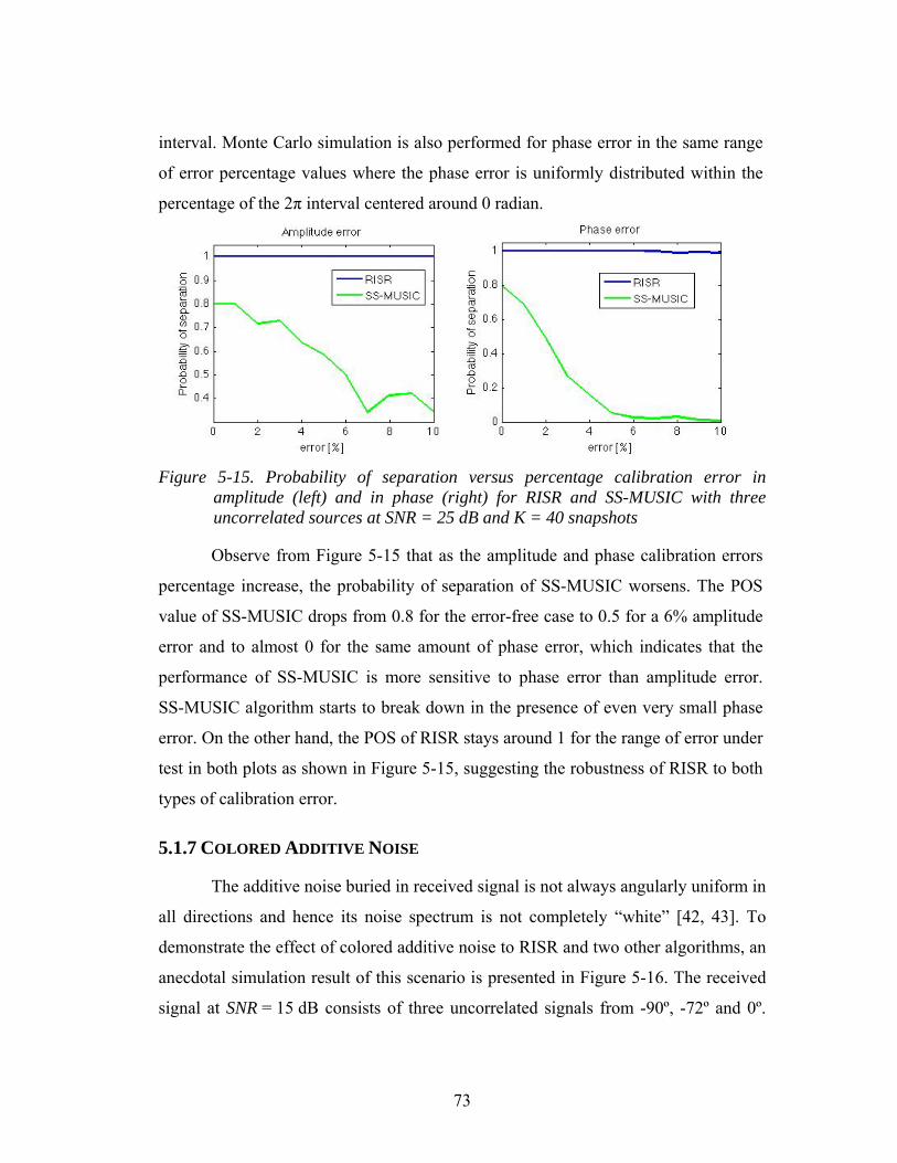
73
interval. Monte Carlo simulation is also performed for phase error in the same range
of error percentage values where the phase error is uniformly distributed within the
percentage of the 2π interval centered around 0 radian.
Figure 5-15. Probability of separation versus percentage calibration error in
amplitude (left) and in phase (right) for RISR and SS-MUSIC with three uncorrelated sources at SNR = 25 dB and K = 40 snapshots
Observe from Figure 5-15 that as the amplitude and phase calibration errors
percentage increase, the probability of separation of SS-MUSIC worsens. The POS
value of SS-MUSIC drops from 0.8 for the error-free case to 0.5 for a 6% amplitude
error and to almost 0 for the same amount of phase error, which indicates that the
performance of SS-MUSIC is more sensitive to phase error than amplitude error.
SS-MUSIC algorithm starts to break down in the presence of even very small phase
error. On the other hand, the POS of RISR stays around 1 for the range of error under
test in both plots as shown in Figure 5-15, suggesting the robustness of RISR to both
types of calibration error.
5.1.7 COLORED ADDITIVE NOISE
The additive noise buried in received signal is not always angularly uniform in
all directions and hence its noise spectrum is not completely “white” [42, 43]. To
demonstrate the effect of colored additive noise to RISR and two other algorithms, an
anecdotal simulation result of this scenario is presented in Figure 5-16. The received
signal at SNR = 15 dB consists of three uncorrelated signals from -90º, -72º and 0º.

74
The colored noise was generated by filtering a spatially “white” signal through a
bandpass filter with the mainlobe centered at 45º. A number of K = 8 data snapshots
are taken for processing and Knoise = 50 snapshots of the pure-noise signal are used to
obtain the noise covariance matrix Rv.
Figure 5-16. Angular spectrum of estimated signal strengths for different algorithms
with 3 uncorrelated signals from -90º, -72º and 0º and addictive noise with mainlobe at around 45º
As shown in the angular spectrum at the bottom left plot in Figure 5-16,
SS-MUSIC estimates only the signal source at 0º correctly. As mentioned before,
SS-MUSIC assumes a white noise spectrum as well as the knowledge of the number
of signal sources, which is three in this simulation, and thus it merges the two sources
at -90º and -72º together as one estimated signal in order to account for the dominant
energy at 45º in the signal space of the covariance matrix. Although the formulation
of FOCUSS resembles that of RISR, the Least Squares approach does not inherently
incorporate the presence of noise into the system model. Without taking noise into
account, the output of the FOCUSS estimator is corrupted by an estimate of the

75
source signal at a noise-concentrated angular direction. Since RISR assumes the
presence of noise in its formulation, the knowledge of the additive noise can be built
into the algorithm. As a result, RISR is able to detect the correct signal sources in the
presence of colored noise with a higher success rate than SS-MUSIC and FOCUSS.
5.1.8 OBSERVATION OF SPARSE SOLUTION CONVERGENCE
The recursive, non-linear nature of RISR makes developing the convergence
proof for the algorithm a challenging task, despite of the successful identification of
signal sources by RISR in a large number of scenarios presented in the Monte Carlo
simulation results in previous sections. However, sparse solution convergence of
RISR can be demonstrated by observing the dominant energy spread in the eigen
spectrum of the filter after the solution of RISR has converged. A few anecdotal
cases are shown in this section to exemplify the convergence of the number of
dominant eigenvalues to the number of signal sources. Since the filter from Equation
(3.4) is not a square matrix, the signal model equation (3.1) is substituted into the
formula for the kth estimate to obtain
( ) ( )
( )SWP
xPxSRSSRSR
vxSRSSRSRx
vxx
vxx
kk
kk
H
HH
HHk
=
=+≈
++=−
−
where
ˆ
ˆ~
1~~
1~~
(5.1)
P is the M×M modified filter matrix of which the eigen spectrum will be
observed in this section. Observe that as k gets large, the eigen space of matrix P is
expected to converge to the a sparse representation.
The first anecdotal case involves a single signal at -90° with SNR = 20 dB and
K = 20 snapshots of received data with the angular spectrum over-sampled by a
factor of 10. The setup of the next two cases are identical to the first except two
uncorrelated signals at -90° and -45° and three uncorrelated signals at -90°, -45° and
0° are present for the second and third cases, respectively. Figure 5-17 below shows
the 10 most dominant eigen values of P at the 15th iteration for all three cases.

76
(a) (b) (c)
Figure 5-17. Ten most dominant eigen values of matrix P at the 15th iteration for the estimation of (a) a single signal source at -90°; (b) two uncorrelated signals at -90° and -45°; (c) three uncorrelated signals at -90°, -45° and 0° with SNR = 20 dB and K = 20
Observe from Figure 5-17 that the number of dominant eigen values in the
eigen spectrum of P for each of the three cases equals the corresponding number of
underlying signal sources. This observation demonstrates that the eigen spectrum of
the solution space of RISR algorithm converges to the most sparse representation,
which is a function of the number of distinct signal sources. Though a proof is not
available, the convergence for RISR is strongly suggested by the three anecdotal
examples.
5.2 SAFFIRE
5.2.1EXPERIMENTAL SETUP AND MEG CONFIGURATIONS
The performance of SAFFIRE is evaluated using computer simulations,
which allow an objective assessment of the dipole localization accuracy for a number
of dipole activation scenarios. Several examples of dipole source reconstruction are
illustrated in the figures in this section to demonstrate the advantages of SAFFIRE
compared to other schemes in terms of their performance. The simulation setup of
dipole localization experiments is based on the physical setup of the MEG sensor
equipments at the Hoglund Brain Imaging Center at the University of Kansas
Medical Center. The human brain volume is evenly divided into 9014 sample grids
for dipole localization. The MEG signals received at the 150 sensors of the

77
biomagnetometer system are simulated for different dipole activation scenarios at a
sampling rate of 600 Hz. Figure 5-18 below illustrates the MEG sensor geometrical
configuration with respect to a brain volume.
Figure 5-18. Physical configuration of 150 MEG sensors relative to the brain.
Sensors are axial gradiometers with 2 detector coils separated by 5 cm. For better visualization, only the lower coil of each sensor is shown.
For each of the 9014 grids throughout the sample space, the leadfield vectors
for only the phi and theta components (in spherical coordinates) of the associated unit
dipole are computed due to the fact that the magnetic fields generated by the radial
component are undetectable outside of the brain in the spherically-symmetric
approximation of the volume conductor [21]. Hence, the size of leadfield matrix B
responsible for dipole activity simulation is 150-by-18028. Each dipole is labeled a
value from 1 to 9014 corresponding to the specific grid in the sample space.
SAFFIRE algorithm used for all the simulation results incorporates
second-stage volumetric constrained processing after the initial SAFFIRE algorithm

78
is performed. The volumetric constrain to the sample space is implemented by first
selecting a group of “active” dipole with at least 30% of the maximum estimated
strength from the original SAFFIRE, then the final set of dipoles is formed by
keeping all dipoles within 2 cm proximity of each dipole from the group of active
dipoles. The leadfield vectors corresponding to the dipoles in the final set is
concatenated to construct Ba,r , the volumetrically constrained leadfield matrix.
5.2.2 SINGLE DIPOLE ACTIVATION
In this section, the performance of SAFFIRE for single dipole activations will
be investigated for three dipoles of various depths in the sample space of the brain.
For all three simulation cases, a dipole activation curve of 2-second duration peaks at
t = 1 s of the activation with a peak dipole strength of 30 nAm and a pulse width of
150 ms. The activation curve shown in Figure 5-19 below is sampled at 600 Hz
which means a total of 1200 samples are collected with a peak at the 600th sample.
Figure 5-19. Activation curve for single dipole activation
The corresponding MEG sensor signal in matrix form of size 150×1200, Y, is
generated using the forward model, which involves multiplying a dipole activation
row vector x by the leadfield vector of the theta component of the activated dipole ri,
b(ri,θ), where the product is then added to a noise vector v. The mathematical
operation is presented in Equation (5.2).

79
vxrbY +=× ),(1200150 θi (5.2)
where the sizes of x, b(ri,θ) and v vectors are 1×1200, 150×1 and 150×1,
respectively. The additive noise magnitude is 10 femto-Tesla which, for example,
results in a SNR of the MEG signal at the peak MGFP to be around 17.44 dB for the
superficial dipole in the first single dipole simulation case. This SNR belongs to the
lower end of the typical SNR range of neural signals.
An example of the MEG sensor measurements at the 150 channels associated
with single dipole activation is displayed in the lower plot of Figure 5-20 and the
averaged power of the signals across sensors, also known as mean global field power
(MGFP) is included in the upper plot of the same figure. The received data sample
with maximum MGFP power is used as the input data for dipole localization of
SAFFIRE algorithm. The criterion for SAFFIRE to estimate the active dipole is by
selecting dipoles with 20% or more of the maximum estimated dipole power
throughout the source space. It is observed that volumetric constrained reprocessing
of SAFFIRE only improves the estimates for single dipole activation slightly.
Figure 5-20. Mean Global Field Power (MGFP, at the top) and the sensors response
of the simulated MEG measurements (at the bottom) corresponding to single dipole activation.

80
Single Dipole Activation, eccentricity of 6.1 cm
The first simulation is performed for a superficial dipole labeled as 8981,
which is 6.1 cm from the center of the brain. Figure 5-21 shows the true dipole in red
as well as the estimated active dipole (in blue) by different algorithms in the 3D brain
map. The input data matrix Y is simulated using Equation (5.2) with the leadfield
vector corresponding to the theta component of dipole 8981. The first algorithm of
which the performance is evaluated is SAFFIRE with single snapshot (K = 1) at the
600th sample of the simulated data. SAFFIRE is repeated to obtain the next set of
results for multiple-time processing with K = 4 snapshots, which is associated with
data from t = 995 ms to t = 1 s. Since FOCUSS and MNE algorithms were only
developed for single snapshot data, only the 600th sample is used for the third and
fourth set of results.
(a)
(b)

81
(c)
(d)
Figure 5-21. The angled (right) and front/top (left) view of the location of the true active dipole 8981 (in red), which is 6.1 cm from the center of the brain, estimated (in blue) by (a) SAFFIRE using K = 1 snapshots at 600th sample; (b) SAFFIRE using K = 4 snapshots centered around 600th sample; (c) FOCUSS using the 600th sample; and (d) MNE (in blue) using the 600th sample with a threshold of 70% of maximum estimated dipole strength
Comparing the results from (a) and (b) in Figure 5-21, both algorithms
accurately estimate the location of the active dipole, indicating that SAFFIRE with
single snapshot data is able to localize the superficial dipole as well as SAFFIRE with
multiple-snapshot processing. FOCUSS in (c) also successfully estimate the
superficial dipole correctly. However, determining the parameters for regularization

82
and norm un-biasing in the FOCUSS algorithm in Equation (2.29) require
considerable amount of effort because they are functions of a number of factors such
as the active dipole location and noise level. Due to the low-resolution nature of MNE
algorithm, a threshold of 70% of maximum estimated dipole strength still results in a
3D dipole estimation map with very poor spatial resolution. MNE is clearly inferior to
other algorithms in terms of spatial precision of dipole localization and is hence not
considered in further performance comparison for algorithms. MNE is also expected
to fail for inner dipoles due to the lack of any scheme for norm-bias adjustment.
Figure 5-22. Dipole strength estimated by SAFFIRE (top left), the neural activity
index resulted from LCMV algorithm (top right), and the dipole strength estimated by MNE (bottom) for activated dipole 8981

83
The plots in Figure 5-22 represent the relative dipole strengths estimated by
different algorithms. Observe that MNE algorithm delivers a “spectrum” with the
worst resolution compared to the other two algorithms as expected. LCMV requires
400 snapshots, an equivalent of 0.667 s duration of data, to construct the data
covariance matrix while only four snapshots, which translates to only 0.0067 s, are
processed for the SAFFIRE algorithm, suggesting the higher temporal resolution
capability of SAFFIRE in dipole localization. A norm-bias adjustment of each dipole
for LCMV is achieved through the neural activity index (NAI), which is the ratio
between the biased estimate of the variance (energy) of the dipole and the estimate of
variance of the noise generated by the same dipole. As shown in Figure 5-22, the plot
of dipole strength estimates by SAFFIRE achieves a remarkably higher level of
sparseness than the NAI plot of LCMV, thus demonstrating the superior spatial
resolution of SAFFIRE. In addition, the greater algorithm efficiency of SAFFIRE can
be easily concluded from the fact that the computation time of LCMV was about
4 minutes, which is 20 times of the 12 seconds required by SAFFIRE.
(a) (b)
Figure 5-23. True activation curve (in green) of dipole 8981 and reconstructed time course of dipole activity (in blue) by (a) SAFFIRE algorithm with K = 4 snapshots and (b) LCMV with 400 snapshots to construct the data covariance matrix
The reconstructed time course of dipole 8981 for SAFFIRE with K = 4
snapshots and for LCMV algorithms are plotted in blue in Figure 5-23. Observe that
compared to LCMV, the time course for SAFFIRE matches slightly better with the

84
true activation curve plotted in green and maintains a lower noise level throughout the
entire time span, suggesting that SAFFIRE can reconstruct cleaner time courses.
Single Dipole Activation, eccentricity of 4.4 cm
The second simulation is performed for a mid-depth dipole labeled as 7952,
with a distance of 4.4 cm from the center of the brain. Figure 5-24 shows the true
dipole in red as well as the estimated active dipole by different algorithms in the 3D
brain map. Again, the MEG sensor data is simulated using Equation (5.2) with the
corresponding data for dipole 7952. The algorithms of which results are shown in
Figure 5-24 are SAFFIRE with single snapshot (K = 1), SAFFIRE with multiple-time
processing (K = 4), and FOCUSS with single snapshot data and same algorithm
parameters as the previous simulation.
(a)
(b)

85
(c)
Figure 5-24. The angled (right) and front/top (left) view of the location of the true active dipole 7952 (in red), which is 4.4 cm from the center of the brain, estimated (in blue) by (a) SAFFIRE using K = 1 snapshots at 600th sample; (b) SAFFIRE using K = 4 snapshots centered around 600th sample; and (c) FOCUSS using the 600th sample
The depth of dipole 7952 creates greater attenuation of magnetic fields, which
consequently worsens the SNR in MEG sensor signal Y than that of dipole 8981 in
the previous simulation. The 3D plot shown in (a) and (b) of Figure 5-24 illustrates
that the SNR gain due to multiple data snapshots enables SAFFIRE to accurately
localize the mid-depth dipole when single-snapshot SAFFIRE can only estimates the
rough location of the same dipole. On the other hand, FOCUSS completely fails to
localize the active dipole and instead, only provide active dipole estimates at
superficial locations as shown in (c). This can be explained by the lack of robust bias
adjustment of the dipole norm and the need to “tune” the parameters of the FOCUSS
algorithm to their optimal values depending on the characteristics of the underlying
dipole. These factors limit the performance of FOCUSS whereas SAFFIRE is free of
such constraints for estimation involving non-superficial dipoles because of the
affine-domain operation and energy normalization at each iteration.

86
(a) (b)
Figure 5-25. True activation curve (in green) of dipole 7952 and reconstructed time course of dipole activity (in blue) by (a) SAFFIRE algorithm with K = 4 snapshots and (b) LCMV with 400 snapshots to construct the data covariance matrix
The reconstructed time course by SAFFIRE shown in Figure 5-25(a) for
dipole 7952 is more noisy than that shown in Figure 5-24(a) for dipole 8981. The
same can also be observed for the time courses by LCMV in Figure 5-24(b) and
Figure 5-25(b). The reason for that is, as mentioned previously, the attenuation of
magnetic field as it travels through the brain increases with dipole depth which causes
the MEG signal SNR to decrease. Compared to LCMV, SAFFIRE produces a
reconstructed time course with a lower noise level over the entire duration as well as
a better-matched pulse around t = 1s.
Single Dipole Activation, eccentricity of 2.0 cm
The last single active dipole simulation is performed for a deep dipole labeled
as 3310, which is 2.0 cm from the center of the brain. Figure 5-26 shows the true
dipole in red as well as the estimated active dipole by different algorithms in the 3D
brain map. Again, the MEG sensor data Y of size 150×1200 is simulated using
Equation (5.2) with the corresponding data for dipole 3310. The algorithms of which
results are shown in Figure 5-26 are SAFFIRE with single snapshot (K = 1) and
SAFFIRE with multiple-time processing (K = 4).

87
(a)
(b)
Figure 5-26. The angled (right) and front/top (left) view of the location of the true active dipole 3310 (in red), which is 2.0 cm from the center of the brain, estimated (in blue) by (a) SAFFIRE using K = 1 snapshots at 600th sample; and (b) SAFFIRE using K = 4 snapshots centered around 600th sample
SAFFIRE with K = 4 snapshot is able to localize accurately an active dipole
very deep in the brain as shown in Figure 5-26(b) whereas with only a single data
vector, SAFFIRE can still estimate the approximate location of dipole 3310.
Although SAFFIRE requires four snapshots to achieve high performance, the
unprecedented temporal resolution of this algorithm demonstrated by accurate
estimation using only an equivalence of 6.67 ms duration of data is a great advantage
over other existing algorithms.

88
Figure 5-27. Dipole strength estimated by SAFFIRE on the left and the neural activity
index resulted from LCMV algorithm on the right for activated dipole 3310
(a) (b)
Figure 5-28. True activation curve (in green) of dipole 3310 and reconstructed time course of dipole activity (in blue) by (a) SAFFIRE algorithm with K = 4 snapshots and (b) LCMV with 400 snapshots to construct the data covariance matrix
Performance degradation of LCMV is illustrated by comparing the NAI plot
of LCMV for dipole 3310 in Figure 5-27 to that for dipole 8981 in Figure 5-22. The
energy is spread out among wider range of dipoles for the deeper dipole, which
effectively lower the spatial resolution of LCMV. SAFFIRE, however, maintains the
sparseness in the solution and return a dominant energy estimate at the correct dipole
location as shown in Figure 5-27, indicating that SNR of sensors signal only affects
the performance of SAFFIRE minimally for single dipole activation.

89
As expected, the reconstructed time courses of dipole 3310 shown in
Figure 5-28 has higher noise level than the corresponding curves for dipole 7952 in
Figure 5-25 for the respective algorithms due to SNR deterioration. Observe that
SAFFIRE reconstructed a time course with significantly lower the noise level and a
more defined pulse curve than the LCMV algorithm. From the comparisons drawn for
the three single dipole activation simulations, SAFFIRE undoubtedly out-performs
LCMV in dipole time course reconstruction.
5.2.3 NEARBY DIPOLE PAIR
In this section, the performance of SAFFIRE is demonstrated for a dipole
simulation of the theta components of a pair of superficial dipoles, which are 1.09 cm
apart and are labeled as 8570 and 8629. Both dipoles have identical activation curve
to the single dipole simulation case and MEG data matrix is simulated using
Equation (5.2) with the data corresponding to the dipole pair. SAFFIRE is performed
with K = 4 snapshots centered around the 603rd sample and volumetric constrained
reprocessing. The sensor data is also processed by LCMV to yield a NAI plot for
comparison with SAFFIRE.
Figure 5-29. Dipole strength estimated by SAFFIRE on the left and the neural activity
index resulted from LCMV algorithm on the right for the dipole pair 8570 and 8629

90
Figure 5-30. Angled (left) and front (right) 3D-view of dipoles 8570 and 8629 (in
red), which are 1.09 cm apart and about 5 cm from the center of the brain, and dipole estimated by SAFFIRE (in blue) using K = 4 snapshots centered around 603rd sample
Figure 5-31. Reconstructed time course of dipole 8570 (left) and 8629 (right) using
SAFFIRE (in blue) and the true dipole activation curve (in red)
It can be observed in Figure 5-29 that the NAI values of the majority of the
dipoles in the NAI plot of LCMV is around 16.5 and the dipoles associated with the
peak NAI do not match with the correct values of 8570 and 8629, indicating that
LCMV fails completely to localize two close-by fully-correlated sources.
On the contrary, the plot of the dipole strength estimated by SAFFIRE shown
in Figure 5-29 contains two peaks at the correct active dipole index of 8570 and 8629
while displaying the high spatial resolution by maintaining the sparseness in the

91
solution “spectrum”. Moreover, the spatial resolution of active dipoles achieved by
SAFFIRE is demonstrated in Figure 5-30, which illustrates accurate localization of
the two close-by dipoles. SAFFIRE also successfully reconstructs the time courses for
the two active dipoles with small noise energy as illustrated in Figure 5-31. The
ability to correctly separate close-by dipole with high spatial resolution as well as to
reconstruct time course proves the distinctly advanced performance of SAFFIRE over
LCMV.
5.2.4 MIRRORED DIPOLE-PAIR IN PRIMARY AUDITORY REGIONS
LCMV is known to break down when spatial correlation or interference is
present in the signal and although the modified version, known as MCMV-CSRS,
can solve such problem, it requires prior knowledge of the location of the interferer.
In this section, the ability of SAFFIRE to handle spatial correlation without any prior
knowledge of the underlying dipole activity is evaluated through the simulation of a
pair of spatially-mirrored dipole located in the primary auditory regions. The dipoles
are labeled as 1088 and 7952 and are both roughly 4.5 cm from the center of the
brain. The activation curve of both dipoles are identical to the single dipole
simulation case and MEG data matrix Y is simulated using Equation (5.2) with the
data corresponding to the dipoles.
Figure 5-32. Angled (left) and front (right) 3D-view of the dipoles in the primary
auditory regions (in red) and dipole estimated by SAFFIRE (in blue) using K = 4 snapshots centered around 600th sample

92
Figure 5-33. Reconstructed time course of dipole 1088 (left) and 7952 (right) in the
auditory region using SAFFIRE (in blue) and the true dipole activation curve (in red)
The spatial correlation robustness of SAFFIRE algorithm is demonstrated
through observations from Figure 5-32 and 5-33. As shown in Figure 5-32, the
locations of both active dipoles are accurately estimated by SAFFIRE. The time
course of the dipole in each primary auditory region reconstructed by SAFFIRE
matches with the true underlying activation curve with small amount of noise as
illustrated in Figure 5-33. The ability for SAFFIRE to handle the case with
mirrored-dipoles in the primary auditory regions is the motivation for testing
SAFFIRE for the ASSR simulation, of which the results are presented next.
5.2.5 AUDITORY RESPONSE
Auditory onset response is an evoked auditory response (EAR) in the primary
and secondary cortex due to brief auditory stimuli presented at short intervals [15].
Studies suggest that EAR can be potentially used for hearing threshold or cognitive
evaluation and measuring the consciousness level of patients undergoing anesthesia.
Accurate reconstruction of the underlying spatio-temporal process of the primary and
secondary cortex is essential to the studies of the neuromagnetic EAR and the effects
induced by other factors. EAR involving short time delay of activation between
dipole pairs in primary and secondary cortex requires very high level of

93
spatio-temporal resolution and as a result, the reconstruction of this type of response
had been a challenging problem in the neuroimaging community with conflicting
results due to the different source reconstruction strategies employed by different
studies.
The configuration of ASSR setup is shown in Figure 5-34 below with two
dipole pairs, which are numbered as 1088, 7952, 613 and 8570, mirrored along the
mid-sagital plane. One mirrored dipole pair is simulated in the regions of the primary
auditory cortex and another in the secondary auditory cortex. The separations
between dipoles 1088 and 613 in the left cerebral hemisphere and that between
dipoles 7952 and 8570 in the right cerebral hemisphere are 1.52 cm and 1.65 cm,
respectively. As illustrated in Figure 5-35, the dipole activation curves of all four
dipoles are identical except that the peaks of activation curves for the secondary
cortex are delayed by 50 ms, or 30 samples, from those in the primary cortex. Peak
dipole strength is 30 nAm and the noise magnitude is 10-15 T.
Figure 5-34. Locations of the dipole pairs in primary cortex (red) and secondary
cortex (green) for the ASSR simulation

94
Figure 5-35. Activation curves of primary and secondary auditory regions with peaks
at t = 1 and 1.05 s (top left), the mean global field power of the received signals (top right) and the MEG sensors response of all 150 channels (bottom left)
Methods
The MEG sensor signals sampled at 600 Hz are generated by summing the
MEG responses corresponding to the activation curve of each of the four dipoles
computed using Equation (5.2). SAFFIRE algorithm is used in a manner similar to an
overlapped sliding window for the data set of 78 samples from t = 962 ms (578th
sample) to t = 1.09 s (655th sample). At each estimation interval, K = 4 consecutive
data snapshots are processed to yield an estimate and hence producing 75 estimates.
Besides the original SAFFIRE algorithm, SAFFIRE with volumetric-constrained
reprocessing as well as 3-of-5 detection are also carried out at each estimation
interval for performance comparison. For simplicity, SAFFIRE with

95
volumetric-constrained reprocessing is interchanged with SAFFIRE-2 in the rest of
this section.
In order to remove the few occurrences of improbable estimates such as split
dipoles or active dipole that only occurs for 1 sample (1.7 ms), the 3-of-5 detection is
applied, also as an overlapped sliding window, to the output of SAFFIRE-2 and is
defined as follows: for each group of five consecutive estimates, if a dipole
considered as active (with at least 30% of the maximum estimated strength) for three
or more of those five estimates, the dipole is counted as active. Since for each group
of five estimates, one 3-of-5 detector estimate is produced, the total number of
estimates after applying 3-of-5 detection is 71, four less than that of the other two
methods.
Results
Three stages of estimated dipole activity are identified after observing the
temporal progression of the dipole estimate locations for each of the three methods.
The first and third stage corresponds to the period when the true dipole pair in the
primary cortex and secondary cortex, respectively, is successfully localized. The
second stage, which typically takes place between the peaks of the primary and
secondary activation curves, is the transition interval where the dipoles estimated at
locations between the primary and secondary cortices.
It is found from the activation curves that the period over which the power of
the dipole associated with the primary activation is at least 20% of its maximum is
from t = 968 ms (582nd sample) to t = 1.032 s (620th sample), whereas the period
corresponding to the secondary activation is from t = 1.018 ms (612rd sample) to
t = 1.082 s (650th sample). In order to compare the performance of the three different
reconstruction methods, the ideal values of time indices will be referred to, which are
listed in Table 5-1 below. Note that the ideal time period for the second stage is when
the primary and secondary activation curves overlap.

96
Table 5-1. Ideal time indices for the first to third stages of ASSR estimation. The bracket value is the sample index corresponding to the time
Ideal time First stage begins 968 ms (582) Second stage begins 1.018 s (612) Third stage begins 1.032 s (620) Third stage ends 1.082 s (650)
The time index at which each stage occurs for the three methods are tabulated
in Table 5-2. Since the estimates in the first or third stage might not be completely
accurate or exact, a “soft” criterion is defined that the localization of a dipole is
determined to be successful only when the estimated dipoles are exactly at or very
close to the true dipole location with no ambiguity that it is in the correct location.
Table 5-2. Estimated time of ASSR dipole localization for the three processing schemes where the bracket value is the sample index corresponding to the time
SAFFIRE SAFFIRE-2 3-of-5 detector
First stage begins 980 ms (589) 968 ms (582) 968 ms (582) Second stage begins 997 ms (599) 1.002 s (602) 1.002 s (602) Third stage begins 1.045 s (628) 1.045 s (628) 1.043 s (627) Third stage ends 1.077 s (647) 1.088 s (654) 1.080 s (652)
Observe from Table 5-2 that the time indices defining the boundary of the
three stages matches better with the ideal case for SAFFIRE-2 than for the original
SAFFIRE. The SAFFIRE-2 and ideal time index for the beginning of the first stage
are both 582, which are 7 snapshots before the corresponding time index for
SAFFIRE. Compared to the ideal duration of 8 snapshots for the second stage,
SAFFIRE-2 with 26 snapshots is closer to ideal than SAFFIRE with 29 snapshots.
Although 3-of-5 detector provides very little improvement over SAFFIRE-2
in terms of the time indices for defining the stages, it delivers cleaner 3D dipole
localization images during the second stage where the dipoles “migrate” from
primary to secondary cortex and during the time period outside of any of the three
stages due to low SNR. Three example sets of the dipole localization 3D plots

97
corresponding to each of the three stages are demonstrated in Figures 5-36, 5-37 and
5-38 below along with the MGFP plots for results of which 3-of-5 detector is applied.
Figure 5-36. An example of the first stage. Top: true dipoles (in red) and the dipole
locations estimated by SAFFIRE-2 with 3-of-5 detector (in blue) in 3D plot for data at around t = 972 ms (584th sample); bottom: MGFP plot from t = 968 ms to t = 1.085 with primary and secondary activation curves which are out of scale. The black vertical line indicates t = 972 ms on the time axis

98
Figure 5-37. An example of the second stage. Top: true dipoles (in red) and the
dipole locations estimated by SAFFIRE-2 with 3-of-5 detector (in blue) in 3D plot for data at around t = 1.025s (616th sample); bottom: MGFP plot from t = 968 ms to t = 1.085 with primary and secondary activation curves which are out of scale. The black vertical line indicates t = 1.025 s on the time axis

99
Figure 5-38. An example of the third stage. Top: true dipoles (in red) and the dipole
locations estimated by SAFFIRE-2 with 3-of-5 detector (in blue) in 3D plot for data at around t = 1.052s (632rd sample); bottom: MGFP plot from t = 968 ms to t = 1.085 with primary and secondary activation curves which are out of scale. The black vertical line indicates t = 1.052 s on the time axis
Observe the MGFP plot within the estimation period in Figure 5-38 that the
power received at MEG sensors at the peak of the primary activation is less than that
at the peak of the secondary activation. This is due to more attenuation associated
with the greater depth of the dipole pair in the primary cortex and hence lower SNR
for the primary activation. Therefore, even though primary and secondary activation
curves are identical with small delay, the third stage is estimated with a longer
duration than the first stage as illustrated in Table 5-2. For the same reason, the
duration of the first stage corresponding to the estimated primary activation is
slightly shorter than that that of the third stage.

100
Figure 5-36 and 5-38 illustrate the accurate dipole localization of the dipole
pairs in the primary and secondary cortices, respectively by SAFFIRE-2 with 3-of-5
detector. The transitional stage example shown in Figure 5-37 associated with data
does not display correct localization of either dipole pairs, the estimates are still
within the auditory cortex in the respective cerebral hemispheres. The temporal
progression of the 3D plot during the transition stage shows the gradual migration of
estimated active dipole from the primary cortex to secondary cortex.
In conclusion, the high temporal and spatial resolution of SAFFIRE enable
the successful reconstruction of the spatio-temporal signal for the ASSR, which can
motivate further neural signal processing to observe other types of neural dynamic
scenarios.
Videos displaying the temporal progression of the dipole localization in 3D
plots for ASSR as well as the three single dipole activation examples are created and
can be requested through email.
5.2.6 TIME-COURSE RECONSTRUCTION WITH INTERFERENCE
Interference, such as energy from other dipole sources, maybe present within
the temporal window of the reconstructed time course, yet outside of the time range
over which data snapshots are taken for constructing the dipole localization filter.
The ability of SAFFIRE to remove such interference with an additional multiple-time
processing is demonstrated through a simulation of two mirrored dipoles of which
the pulses of the dipole activation curves are separated with no overlapping.
The activation curves of the two dipoles in the primary auditory cortex,
numbered as 1088 and 7952, and the MGFP of the MEG sensor signal are shown in
Figure 5-39. The pulse of dipole 7952 is delayed by 500 ms, or 300 samples, from
the pulse of dipole 1088 so that when K = 4 snapshots corresponding to the peak of
MGFP at t = 1 s (601st sample) are processed by SAFFIRE, the activity of the
interferer dipole (7952) does not contribute to dipole strengths estimation. The
resulting 3D plot and the reconstructed time course of the estimated active dipole are
shown in Figure 5-40.

101
Figure 5-39. Activation curves of dipoles 1088 and 7952 in the primary cortex with
peak delay of 500 ms (left) and the MGFP plot of the MEG sensor signal (right)
Figure 5-40 Angled (top left) and front (top right) 3D-view of dipoles 1088 and 7952
in the primary cortex (red) with 500 ms peak delay and the dipole estimated by SAFFIRE (blue). The bottom plot is the reconstructed time course of the estimated dipole 1088 with a false peak at 1.5 s (blue) and the true activation curve (red)

102
Since the data snapshots around t = 1 s consisting of only the activity of
dipole 1088 is selected to construct the filter, SAFFIRE identifies active source at
dipole 1088 though not dipole 7952 as shown in Figure 5-40. The reconstructed time
course of dipole 1088 contains a large peak around t = 1 s as expected and a smaller
peak at t = 1.5 s. If no prior knowledge of the underlying dipole activity is available,
the smaller peak could be a correct dipole pulse but it could also be a false peak due
to activation of other dipoles which are spatially correlated with dipole 1088.
Figure 5-41. Angled (top left) and front (top right) 3D-view of dipoles 1088 and 7952 in the primary cortex (red) with 500 ms peak delay and the dipoles estimated by SAFFIRE (blue). The bottom plots are the reconstructed time course of the dipoles 1088 and 7952 (blue) and the true activation curve (red)

103
The multiple-time processing feature of SAFFIRE can be utilized in an
alternative way to determine the true nature of the second peak. Four additional data
snapshots around the time index associated with the second peak, i.e. t = 1.5 s
(902nd sample), are concatenated with the original four snapshots around t = 1 s to
form a new set of mixed input data for the SAFFIRE algorithm. The 3D plots of the
estimated dipoles from the SAFFIRE reprocessing with mixed input are shown in
Figure 5-41 along with the two reconstructed time courses.
With the MEG data input containing activities of the two dipoles, SAFFIRE
accurately localized the dipoles responsible for the mixed sensor signal as shown in
the upper plots of Figure 5-41. The time courses of the estimated dipoles in the
bottom plots match very well with the associated underlying activation curves.
Observe that the second peak of the reconstructed time course at t = 1.5 s in
Figure 5-40 does not appear in the corresponding plot in Figure 5-41, whereas the
reconstructed time course of the dipole 7952 has a peak at t = 1.5 s. The observations
imply that the second peak in Figure 5-40 was indeed a false peak containing dipole
energy of dipole 7952 due to the spatial correlated of the two dipoles. SAFFIRE filter
can reconstruct dipole time courses only with information embedded in the input data
the filter is constructed with. Intuitively speaking, since the mixed data carries
information of the interferer, SAFFIRE is able to project out the dipole energy
leakage of dipole 7952 from the reconstructed time course of dipole 1088 while the
first SAFFIRE fails in the same regard. The results of this simulation case
demonstrate the ability of SAFFIRE to successfully reconstruct spatially uncorrelated
time courses through a secondary processing with input data containing activities of
potential interferers.

104
CHAPTER 6: CONCLUSIONS AND FUTURE WORK
6.1 Conclusions
The novel algorithm developed for direction of arrival estimation, denoted as
Re-Iterative Super-Resolution (RISR), recursively update the filter through the power
estimates in the formulation until the solution converges to a maximally sparse
solution. The results in Chapter 5 shows that RISR out-performs the algorithms under
comparison in both spatial and temporal resolution. Super temporal resolution
enabled by the single-snapshot processing becomes a major advantage in the
presence of fast-moving targets, whereas finer spatial resolution increases the success
of distinguishing closely-separated sources by the ULA. The temporal correlation
robustness of RISR is a useful property when multiple signal sources are
synchronized. Calibration error at each of the antenna elements is inevitable in
antenna arrays setup and therefore the tolerance of RISR toward such error
demonstrated through simulations is extremely useful in DOA estimation with real
data. The susceptibility to colored noise or interference as well as the ability to
estimate signal strength in addition to the aforementioned advantages reflects the
great potential of the RISR algorithm.
Source AFFine Image REconstruction, an iterative approach based on the
MMSE framework, is a powerful tool for functional neural imaging with
magnetoencephalography signals as shown in the results of a number of dipole
localization simulations. However, SAFFIRE can be applied to inverse modeling
with other imaging techniques, such as magnetocardiography for the heart [44] and
magnetogastrography [45] for the abdomen, provided that accurate forward models
exist. Parametric neural dipole localization algorithms are known for heavy bias in
favor of superficial dipoles. SAFFIRE was shown to produce bias-free estimates in
simulations with activated dipoles of various depths without the need for parameter
adjustment. The spatial resolution achieved by SAFFIRE due to solution sparseness
confines the activate dipole region and, hence, is helpful for separating two close-by

105
dipoles. The exceptional temporal resolution is another advantage of SAFFIRE that
allows the observation of neural evoked response dynamics in finer details. The
unprecedented spatio-temporal resolution, temporal correlation robustness,
independence of statistical prior knowledge and the effective dipole activity time
course reconstruction of SAFFIRE together build the success in reconstructing the
multiple sources of auditory evoked responses which is a difficult problem in the
functional imaging community.
In spite of the similarities between the algorithms, such as the framework on
which they are based and their recursive natures, RISR and SAFFIRE are two
distinct approaches with a few principal differences. First of all, SAFFIRE is specific
for inverse modeling of the biological process while RISR is applied to the more
general DOA estimation. The signal model of RISR assumes far-field signals
impringing on the ULA whereas the conformed array antenna configuration of
SAFFIRE does not make such assumption. Lastly, SAFFIRE incorporates energy
normalization and affine-transformed space operation at each iteration into the
algorithm to alleviate the effects of matrix ill-conditioning, which is not a problem
with the DOA estimation for the RISR algorithm.
6.2 Future Work
The evaluation of RISR algorithm shown in Chapter 5 was based on the
simulation of sources with equal signal strengths. Therefore, other aspects of the
algorithm, such as the signal sources dynamic range, distributed sources scenarios
and real data processing, can be the next steps of investigation. The RISR is built
upon a MMSE framework with a two-dimensional signal model for the azimuth
angle. An extension of RISR into three-dimensional DOA estimation can be explored
by considering a signal model that incorporates azimuth and elevation of the source
signals.
The purpose of applying a 3-of-5 detector to a dipole activation response
reconstructed by SAFFIRE is analogous to smoothing the spatial dipole estimates

106
across time in order to eliminate “short-lived” estimates, due to the low physical
probability of such activation duration. This temporal averaging of spatial
information is an example of space-time coupling processing, which enables
information extraction from the relationship between the current and additional
dimensions. Instead of post-processing, the first order information between space and
time, such as the slope of activation curve of a detected dipole, might possibly be
incorporated into the filter formulation to increase the accuracy of the overall
reconstructed response.
SAFFIRE was shown to accurately localize dipole activities and reconstruct
time course of the dipole activities by the results of a limited number of scenarios.
Therefore, other scenarios, such as dipole activation curve shape and distributed
dipole activity, can be simulated to examine the performance of the algorithm. Also,
SAFFIRE is still yet to be tested on real experimental MEG data of the auditory
evoked responses.
In spite of the disadvantages of other medical imaging techniques as
discussed in the background section, some related research has been conducted for
fMRI constrained MEG signal processing with other algorithms [46]. This approach
should be investigated further since other imaging methods offer complementary
information that will potentially increase the performance of SAFFIRE.
The sensor signals in the forward model from which SAFFIRE is derived can
be substituted with ones related to other physical phenomena, for example,
electroencephalography, magnetocardiography and magnetogastrography. The
unprecedented spatio-temporal resolution of SAFFIRE algorithm can benefit the
estimation of the underlying activities with higher accuracy and precision.
The applications of the recursive MMSE framework in radar adaptive pulse
compression, direction of arrival estimation and functional neural imaging have been
shown to achieve excellent performance. While the algorithms, depending on the
application, might require different adjustment, the common formulation of the basic
RMMSE filter should allow flexible application to other types of signal estimation.

107
REFERENCES
[1] Blunt, S. D., Gerlach, K., “Adaptive pulse compression via MMSE estimation,” IEEE Transactions on Aerospace and Electronic Systems, vol. AES-42, no. 2, pp. 572-584, April 2006. [2] Nikolakopoulos, K. V., Anagnostou, D., Christodoulou, C. G., and Chryssomallis, M. T., “Estimation of direction of arrival for coherent signals in wireless communication systems,” IEEE Antennas and Propagation Society International Symposium, vol. 1, pp. 20-25, June 2004. [3] Jeffs, B., Leahy, R., and Singh, M., “An Evaluation of Methods for Neuromagnetic Image Reconstruction,” IEEE Transactions on Biomedical Engineering, vol. BME-34, no. 9, pp. 713-723, Sept. 1987. [4] Krim, H., and Viberg, M., “Two decades of array signal processing research: the parametric approach,” IEEE Signal Processing Magazine, vol. 13, no. 4, pp. 67-94, Jul 1996 [5] Van Trees, Harry L., Optimum Array Processing: Part IV of Detection, Estimation, and Modulation Theory, John Wiley and Sons Inc, 2002. [6] Stoica, P., and Nehorai, A., “MUSIC, maximum likelihood, and Cramer-Rao bound,” IEEE Transactions on Acoustics, Speech, and Signal Processing, vol. 37, no. 5, pp. 720-741, May 1989. [7] Schmidt, R. O., “Multiple emitter location and signal parameter estimation,” IEEE Transactions on Antennas and Propagation, vol. 34, no. 3, pp. 276-280, 1986. [8] Shan, T. J., Wax, M., and Kailath, T., “On spatial smoothing for direction-of-arrival estimation of coherent signals,” IEEE Transactions on Acoustics, Speech, and Signal Processing, vol. ASSP-33, no. 4, pp. 806-811, Aug. 1985. [9] Gorodnitsky, I. F., and Rao, B. D., “Sparse signal reconstruction from limited data using FOCUSS: a recursive weighted norm minimization algorithm,” IEEE Transactions on Signal Processing, vol. 45, no. 3, pp. 600-616, 1997. [10] Gorodnitsky, I. F., George, J. S., and Rao, B. D., “Neuromagnetic source imaging with FOCUSS: a recursive weighted minimum norm algorithm,” Journal of Electroencephalography and Clinical Neurophysiology, pp. 231-251, 1995. [11] Van Veen, B. D., Van Drongelen, W., Yucktman, M., and Suzuki, A., “Localization of brain electrical activity via linearly constrained minimum variance

108
spatial filtering,” IEEE Transactions on Biomedical Engineering, vol. 44, no. 9, pp. 867-880, Sept. 1997. [12] Van Veen, B. D., Joseph, J., Hecox, K. E., “Method and apparatus for localization of intracerebral sources of electrical activity,” United States Patent 5,263,488, November 23, 1993. [13] Widrow, B., Duvall, K. M., Gooch, R. P., and Newman, W. C., “Signal cancellation phenomena in adaptive antennas: causes and cures,” IEEE Transactions on Antennas and Propagation, vol. AP-30, no. 5, pp. 469-478, July 1982. [14] Evans, J. E., Johnson, J. R., and Sun, D. F., “High resolution angular spectrum estimation techniques for terrain scattering analysis and angle of arrival estimation,” Proceedings of 1st ASSP Workshop on Spectral Estimation, pp. 134-139, 1981 [15] Popescu, M., Popescu, E. A., Chan, T., Blunt, S., Lewine J. D., “Spatio-temporal reconstruction of bilateral auditory steady-state responses using MEG beamformers,” IEEE Transactions on Biomedical Engineering, vol. 55, no. 3, Mar. 2008, pp. 1092 - 1102. [16] Gabriel, W. F., “Spectral analysis and adaptive array superresolution techniques,” Proceedings of the IEEE, vol. 68, no. 6, pp. 654- 666, June 1980. [17] Zimmerman, J. E., Thiene, P., and Harding, J. T., “Design and operation of stable rf-based superconducting point-contact quantum devices and a note on the properties of perfectly clean metal contacts,” Journal of Applied Physics, vol. 41, pp. 1572-1580, 1970. [18] Cohen, D., “Magnetoencephalography: Detection of the brain’s electrical activity with a superconducting magnetometer,” Science, vol. 175, pp. 664-666, 1972. [19] Drawing of the anatomical structure of a neuron: “Nerve Cells and Neurotransmission”, http://www.drugabuse.gov/MOM/TG/momtg-introbg.html [20] Scherg, M., and Von Cramon, D., “Evoked dipole source potentials of the human auditory cortex”, Electroencephalography Clinical Neurophysiology, vol. 65, 1986, pp. 344-360. [21] Ilmoniemi, R. J., Hämäläinen, M. S., and Knuutila, J., “The forward and inverse problems in the spherical model,” Biomagnetism: Applications and Theory, Pergamon, New York, pp. 278-282, 1985. [22] Pechura, C. M., and Martin, J. B., Eds., Mapping the Brain and its Functions, National Academy, Washington, DC., 1991.

109
[23] Hamalainen, M. R., Hari, R., Ilmoniemi, R. J., Knuutila, J. and Lounasmaa, O., “Magnetoencephalography - theory, instrumentation, and applications to noninvasive studies of the working human brain,” Reviews of Modern Physics, vol. 65, no. 2, pp. 413-497, Apr. 1993. [24] Lauterbur, P. C., “Image formation by induced local interactions: Examples employing nuclear magnetic resonance,” Nature, vol. 242, pp. 190-191, Mar. 1973. [23] Hinz, T., 1988, “Utilization of reconstruction algorithms in transmission and emission computed tomography,” Imaging Techniques in Biology and Medicine, Academic Press, New York, pp. 257-299, 1988. [26] Damadian, R., “Apparatus and method for detecting cancer in tissue,” U.S. Patent 3,789,832, 1972. [27] Hinshaw, W. S., and Lent, A. H., “An introduction to NMR imaging: From the Bloch equation to the imaging equation,” Proceedings of IEEE, vol. 71, pp. 338-350, 1983. [28] Knoll, G. F., “Single-photon emission computed tomography,” Proceedings of IEEE, vol. 71, pp. 320-329, 1983. [29] ter-Pogossin, M. M., Phelps, M. E., Hoffman, E. J., and Mullani, N. A. “A positron emission transaxial tomography for nuclear medicine imaging (PETT),” Radiology, vol. 114, pp. 89-98, 1975. [30] Kessler, R. M., Partain, C. L., Price, R. R., and James, E., “Positron emission tomography: Prospects for clinical utility,” Investigative Radiology, vol. 22, pp. 529-537, 1987. [31] Belliveau, J. W., Kennedy, D. N., McKinstry, R. C., Buchbinder, B. R., Weisskoff, R. M., Cohen, M. S., Vevea, J. M., Brady, T. J., and Rosen, B. R., “Functional mapping of the human visual cortex by magnetic resonance imaging,” Science, vol. 254, pp. 716-719, 1991. [32] Weiskopf, N., Sitaram, R., Josephs, O., Veit, R., Scharnowski, F., Goebel, R., Birbaumer, N., Deichmann, R., Mathiak, K, “Real-time functional magnetic resonance imaging: methods and applications,” Magnetic Resonance Imaging, vol. 25, no. 6, pp. 989-1003, 2007.

110
[33] Cox, R. W., Jesmanowicz, A., and Hyde, J. S., “Real-time functional magnetic resonance imaging,” Magnetic Resonance in Medicine, vol. 33, no. 2, pp. 230-236, 1995. [34] Sarvas, J., ”Basic mathematical and electromagnetic concepts of the biomagnetic inverse problem,” Physics in Medicine and Biology, vol. 32, pp. 11-22, 1987. [35] Kay, S. M., Fundamentals of Statistical Signal Processing: Estimation Theory, Prentice-Hall, Upper Saddle River, New Jersey, pp. 219-286 and 344-350, 1993. [36] Haykins, Simons, Adaptive Filter Theory, Prentice Hall, 2001 [37] Hamalainen, M., Ilmoniemi, R., “Interpreting measured magnetic fields of the brain: estimates of current distributions,” Technical Report, Helsinki University of Technology, TKK-F-A559, 1984. [38] Mosher, J. C.; Lewis, P. S.; Leahy, R. M., “Multiple dipole modeling and localization from spatio-temporal MEG data,” IEEE Transactions on Biomedical Engineering, vol. 39, no. 6, pp. 541 – 557, June 1992. [39] Herdman, A. T., Wollbrink, A., Chau, W., Ishii, R., Ross, B., Pantev, C., and Ross, R., “Determination of activation areas in the human auditory cortex by means of synthetic aperture magnetometry,” NeuroImage, vol. 20, no. 2, pp. 995-1005, Oct. 2003. [40] Dalal, S. S., Sekihara, K., and Nagarajan, S. S., “Modified beamformers for coherent source region suppression,” IEEE Transaction on Biomedical Engineering, vol. 53, no. 7, Jul. 2006, pp. 1357 – 1363. [41] Willis, N. J., Bistatic Radar, SciTech Publishing Inc., Raleigh, NC, 2005. [42] Li, F., and Vaccaros, R. J., “Performance degradation of DOA estimators due to unknown noise fields,” IEEE Transactions on Signal Processing, vol. SP-40, no. 3, pp. 686-689, March 1992. [43] Wong, K. M., Reilly, J. P., Wu, Q., and Qiao, S., “Estimation of the directions of arrival of signals in unknown correlated noise, Parts I and II,” IEEE Transactions on Signal Processing, vol. SP-40, pp. 2007-2028, Aug. 1992. [44] Nenonen, J., Purcell, C. J., Horacek, B. M., Stroink, G., and Katila, T., “Magnetocardiographic functional localization using a current dipole in a realistic torso,” IEEE Transactions on Biomedical Engineering, vol. 38, pp. 658-664, 1991.

111
[45] Irimia, A., Richards, W. O., Bradshaw, L. A., “Magnetogastrographic detection of gastric electrical response activity in humans,” Physics in Medicine and Biology, vol. 51, pp. 1347-1360, 2006 [46] Liu, A. K., Belliveau, J. W. and Dale, A. M., “Spatiotemporal imaging of human brain activity using functional MRI constrained magnetoencephalography data: Monte Carlo simulations,” Proceedings of National Academy Science U S A, vol. 95, pp. 8945-8950, 1998.