Active Voice Control: An Implementation of Active Noise Control for

Canceling Speech

Except where reference is made to the work of others, the work described in this thesis ismy own or was done in collaboration with my advisor. This thesis does not include

proprietary or classified information.

Christopher Rose

Certificate of Approval:

Vishwani AgrawalProfessorDepartment of Electrical and ComputerEngineering

James R. HansenDirectorUniversity Honors College

Active Voice Control: An Implementation of Active Noise Control for

Canceling Speech

Christopher Rose

A Thesis

Submitted to the

Auburn University Honors College

In Partial Fulfillment of the

Requirements for

University Honors Scholar

Auburn, AlabamaJune 7, 2007

Active Voice Control: An Implementation of Active Noise Control for

Canceling Speech

Christopher Rose

Permission is granted to Auburn University to make copies of this thesis at its discretion,upon the request of individuals or institutions and at their expense. The author reserves

all publication rights.

Signature of Author

Date of Graduation

iii

Vita

Christopher J. Rose was born in Huntsville, Alabama, on August 11, 1985. He attended

elementary schools in the Huntsville City School District and graduated from Grissom High

School with honors in 2003. The following August, he entered Auburn University where he

is currently seeking a double major in Electrical Engineering and Electrical and Computer

Engineering. His extracurricular activities include membership in Eta Kappa Nu and the

Auburn Knights Orchestra. In the fall of 2007, he will begin seeking a master’s degree in

Electrical Engineering.

iv

Thesis Abstract

Active Voice Control: An Implementation of Active Noise Control for

Canceling Speech

Christopher Rose

Bachelor of Electrical Engineering, June 7, 2007

54 Typed Pages

Directed by Vishwani Agrawal

New developments in active noise control (ANC) have led to commercial products such

as noise canceling headphones and low engine sound airplane cockpits. These products

rely on adaptive filters to eliminate noise by playing the antinoise of the original sound.

Similarly, this strategy can be applied to voice to cancel unwanted speech in the open air.

In some cases, the speech must be preserved for the speaker to communicate and canceled in

the surrounding environment for unwanted listeners. This research introduces active voice

control (AVC) in canceling speech and discusses some of the difficulties in implementing

AVC in an open air environment.

v

Acknowledgments

I would first like to thank my adviser, Dr. Vishwani Agrawal, for his guidance through-

out the process of creating this thesis and for encouraging me to participate in my first

symposium. I would also like to thank Darrel Hankerson for his help in a modification of

the aums.sty file to match the Honors Congress specifications. Finally, I would like to thank

my family for their endless support.

vi

Style manual or journal used Journal of Approximation Theory (together with the style

known as “aums”). Bibliography follows van Leunen’s A Handbook for Scholars.

Computer software used The document preparation package TEX (specifically LATEX)

together with the departmental style-file aums.sty.

vii

Table of Contents

List of Figures ix

1 Introduction 1

2 Literature Survey on Active Noise Control 32.1 Origins . . . . . . . . . . . . . . . . . . . . . . . . . . . . . . . . . . . . . . . 32.2 Physical Design of the ANC System . . . . . . . . . . . . . . . . . . . . . . 5

2.2.1 Single Sensor and Actuator Scheme . . . . . . . . . . . . . . . . . . 72.2.2 Multiple Sensors and Actuators Scheme . . . . . . . . . . . . . . . . 8

2.3 Adaptive Algorithms . . . . . . . . . . . . . . . . . . . . . . . . . . . . . . . 92.3.1 Finite Impulse Response . . . . . . . . . . . . . . . . . . . . . . . . . 102.3.2 Infinite Impulse Response . . . . . . . . . . . . . . . . . . . . . . . . 13

2.4 Limitations of Active Noise Control . . . . . . . . . . . . . . . . . . . . . . . 172.5 Commercial Products . . . . . . . . . . . . . . . . . . . . . . . . . . . . . . 20

2.5.1 ANC Headphones . . . . . . . . . . . . . . . . . . . . . . . . . . . . 202.5.2 Other Products . . . . . . . . . . . . . . . . . . . . . . . . . . . . . . 24

3 Active Voice Control 283.1 Differences between Active Noise Control and Active Voice Control . . . . . 283.2 Difficulties with Voice Control . . . . . . . . . . . . . . . . . . . . . . . . . . 293.3 Applications . . . . . . . . . . . . . . . . . . . . . . . . . . . . . . . . . . . . 33

3.3.1 Mobile Cellular Phone Booth . . . . . . . . . . . . . . . . . . . . . . 333.3.2 Residual Voice Cancellation . . . . . . . . . . . . . . . . . . . . . . . 34

4 Simulation 364.1 The Active Sound Control Simulink Diagram . . . . . . . . . . . . . . . . . 36

4.1.1 AVC with a Single Tone . . . . . . . . . . . . . . . . . . . . . . . . . 374.1.2 AVC with Recorded Speech . . . . . . . . . . . . . . . . . . . . . . . 38

5 Conclusion 41

Bibliography 42

Appendix 43

viii

List of Figures

2.1 A figure from Paul Lueg’s 1936 Patent for ANC [7]. . . . . . . . . . . . . . 4

2.2 Difference between disturbance and ASC sound fields in an open air environ-ment [14]. . . . . . . . . . . . . . . . . . . . . . . . . . . . . . . . . . . . . . 8

2.3 LMS block diagram [4]. . . . . . . . . . . . . . . . . . . . . . . . . . . . . . 10

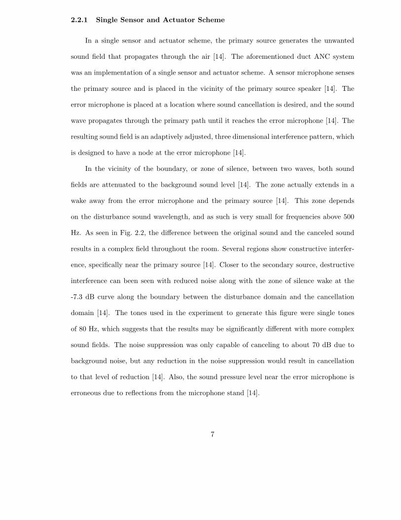
2.4 ANC block diagram [9]. . . . . . . . . . . . . . . . . . . . . . . . . . . . . . 12

2.5 Modified filtered-X LMS block diagram [12]. . . . . . . . . . . . . . . . . . . 13

2.6 Modified filtered-X structure for RLS [12]. . . . . . . . . . . . . . . . . . . . 14

2.7 Gradient lattice block diagram [6]. . . . . . . . . . . . . . . . . . . . . . . . 16

2.8 Convergence comparison between (a)GL, (b) FULMS, and (c) FVLMS algo-rithms [6]. . . . . . . . . . . . . . . . . . . . . . . . . . . . . . . . . . . . . . 17

2.9 Power spectra for engine noise at 3700 rpm (dotted line) and the noise afterANC(solid line) [13]. . . . . . . . . . . . . . . . . . . . . . . . . . . . . . . . 18

2.10 Noise canceling headphone using ANC [3]. . . . . . . . . . . . . . . . . . . . 21

2.11 Locations for an error microphone for ANC headphones [13]. . . . . . . . . 22

2.12 Integrated audio and ANC system block diagram [5]. . . . . . . . . . . . . . 23

2.13 Noise spectrum comparison for ANC and non-ANC systems from siren dis-turbance [5]. . . . . . . . . . . . . . . . . . . . . . . . . . . . . . . . . . . . . 25

2.14 Noise spectrum comparison for ANC and non-ANC Systems from enginedisturbance [5]. . . . . . . . . . . . . . . . . . . . . . . . . . . . . . . . . . . 26

3.1 Overhead view of the preservation of speech due to the wake of silence. . . . 31

4.1 Simple Simulink diagram for antinoise cancellation of a sinusoid. . . . . . . 37

4.2 Active voice control Simulink diagram for single tone cancellation. . . . . . 38

ix

4.3 Acoustic environment for single tone cancellation. . . . . . . . . . . . . . . . 39

4.4 Active voice control Simulink diagram for recorded speech cancellation. . . 39

4.5 Acoustic environment Simulink diagram for recorded speech cancellation. . 40

1 Acoustic Noise Cancellation Simulink Diagram [8] . . . . . . . . . . . . . . 44

2 Acoustic Environment Simulink Diagram for Active Noise Control [8] . . . . 44

x

Chapter 1

Introduction

One of the most researched subjects in signal processing and acoustics is active noise

control. This system uses sensors, microphones, and digital signal processing boards to

create the antinoise of a sound. The system can create the antinoise by manipulating the

error signal with the adaptive filters of the digital signal processor, thereby compensating in

any change in the plant of the system model. Depending on the application, both feedback

control and feedforward control can be used in active noise control. Success has been seen

in such applications as headsets and cockpits of aircraft to cancel low frequency noise.

Success in the mid to upper range of audible frequency, however, has been limited to very

small regions. Currently, passive systems are most often used to control sound in the upper

frequency range.

By extending active noise control into higher frequencies, sound from speech can be

actively controlled. This system, presented in this paper as active voice control (AVC),

can be used in a range of applications to prevent unwanted vocal communication. In most

of these applications, the speech signal itself must be preserved for communication to an

intended audience while isolating it from unwanted listeners. Therefore, AVC seeks not to

cancel the entire speech as ANC does for noise but to preserve some aspect of it.

This paper presents a AVC as a theoretical replacement of passive systems to control

speech. A simulation of AVC has been developed which uses ANC to cancel unwanted

speech. This simulation, however, does not take into consideration the geometry nor the

actual conditions of the surrounding environment. The difficulties with implementing AVC

1

in real systems, such as the limitations of ANC itself and the ethical responsibilities of

silencing someone’s speech, prevent AVC from being realized in a real system. Only after

ANC has been extended into the bulk of vocal frequency range can AVC be successfully

implemented.

2

Chapter 2

Literature Survey on Active Noise Control

2.1 Origins

Active control was first theorized by Paul Lueg in 1936 in U.S. Patent Number 2,043,416 [7].

His patent describes measuring the sound field with a microphone, electrically manipulating

the resulting signal, and then feeding it to an electroacoustic secondary source [4]. As seen

in Figure 2.1 of Lueg’s patent, the sound is considered to travel as plane waves in a duct

from a primary source A [4]. The microphone, M, detects the sound wave and supplies the

excitation to the electronic controller, V, to drive the loudspeaker at L [4]. The loudspeaker

produces a sound wave that is out of phase with the primary source’s acoustic wave [4].

Destructive interference is created from the superposition of the acoustic wave of the loud-

speaker and the wave of the original source [4]. This concept is the basis for today’s active

noise control; however, at that time Lueg could not practically demonstrate his patent.

Seventeen years later, Harry Olson and Everet May published another paper which

describes another system for active noise control [4]. In contrast with Lueg’s paper which

used prior knowledge of the signal from the detecting microphone (feedforward control),

Olson and May’s strategy needed no prior knowledge of the sound field [4]. Instead, it

used a feedback method to cancel sound by feeding back the signal from a much closer

microphone to a second loudspeaker [4].

A few years later in 1956, William Conover was working on acoustic noise reduction

from power distribution transformers at Generic Electric Company [3]. The magnetostric-

tion in the transformer made it hum at even harmonics of the line frequency [3]. This

3

Figure 2.1: A figure from Paul Lueg’s 1936 Patent for ANC [7].

periodic nature of the sound allowed Conover to avoid using a microphone and instead

generate a reference signal which has the same frequency components as the primary noise.

These reference signals were derived from full-wave rectified version of the line voltage and

bandpass filtered to obtain the even harmonics [3]. Only the amplitude and phase of this

reference signal need to be varied by the controller of the system [4]. The objective of his

design was to cancel the pressure in a particular direction away from the transformer, such

as a nearby house [4]. He carried out the cancellation using a manual controller, which

he adjusted to compensate for winds and temperature changes [4]. The suggestions in his

4

paper to use an automatic control system as well as multiple secondary loudspeakers and

monitoring microphones were very important in the future development of ANC [4].

Due to the lack of capable technology in the 1930’s and 1950’s, ANC was not possi-

ble until modern computers became available. As such, the study of active noise control

was silent until 1975, when Kido first used digital techniques to achieve the precise bal-

ance required for feedforward active control [4]. As digital computers became faster and

more common, active noise control has become much more practical, and ANC became a

mainstream research topic in the 1970’s and 1980’s [11]. In 1980, the well known filtered-x

least mean squares algorithm was developed by Morgan and also independently by Widrow

in 1981 and now figures prominently in recent active noise control research [12, 9] To-

day, researchers publish technical articles on active control at a rate of several hundred per

year [11]. Dozens of companies now specialize in active control products such as headphones,

and universities and government research laboratories are actively involved in active noise

control research [11].

2.2 Physical Design of the ANC System

ANC systems consist primarily of four major parts: the plant, sensors, actuators, and

controller. The plant is the physical system to be controlled, such as the compartment

in a vehicle or the air traveling through a duct [11]. The sensors are the microphones, ac-

celerometers, and other devices that sense the disturbance and monitor how well the control

system is performing [11]. The actuators are the devices that physically change the system

such as the speakers [11]. Finally, the controller is the digital signal processor that uses

the information from the sensors to instruct the actuators to achieve noise cancellation [11].

Each of these components are the building blocks for a complete ANC system.

5

ANC itself works on the principle of destructive interference between the primary dis-

turbance field heard as unwanted noise and the secondary field which is generated from

control actuators [2]. In the simplest system, the disturbance field can be a simple sine

wave, and the secondary field is the same sine wave but 180 degrees out of phase. The

resulting superposition of the two waves is no sound at all. The human ear responds mainly

to the mean square value of the pressure it registers. So the quantity that most active

control systems are designed to minimize is the mean square value of this error signal [3].

Since most if not all systems have complex frequencies and waveforms, the secondary field

is much more complex than merely 180 degrees out of phase. Moreover, the plant model

usually changes dynamically, resulting in a system which requires an adaptive filter or many

microphones to determine the current disturbance field.

An arrangement of two domains, one the disturbance and the other the cancellation

noise, can be replaced by two sets of simple sources acting on the boundary between the two

domains [14]. If a set of active sources is identical to the set of disturbance sources but in

antiphase, or 180 degrees out of phase, then no sound will be present at the boundary [14].

Additionally, if the boundary is placed so that it isolates the disturbance domain and the

cancellation domain from the silent domain, then the effects of the disturbances and active

sources will not affect the silent domain [14]. This boundary is called the wall of silence and

serves as a wall between the noise source and the silent domain [14]. The boundary would

ideally have an infinite number of anti-phase sources to achieve this theoretical level of per-

formance [14]. The number of actuators can make a significant impact on the performance

and design of an ANC system. The next section describes a system with a single actuator,

or microphone.

6

2.2.1 Single Sensor and Actuator Scheme

In a single sensor and actuator scheme, the primary source generates the unwanted

sound field that propagates through the air [14]. The aforementioned duct ANC system

was an implementation of a single sensor and actuator scheme. A sensor microphone senses

the primary source and is placed in the vicinity of the primary source speaker [14]. The

error microphone is placed at a location where sound cancellation is desired, and the sound

wave propagates through the primary path until it reaches the error microphone [14]. The

resulting sound field is an adaptively adjusted, three dimensional interference pattern, which

is designed to have a node at the error microphone [14].

In the vicinity of the boundary, or zone of silence, between two waves, both sound

fields are attenuated to the background sound level [14]. The zone actually extends in a

wake away from the error microphone and the primary source [14]. This zone depends

on the disturbance sound wavelength, and as such is very small for frequencies above 500

Hz. As seen in Fig. 2.2, the difference between the original sound and the canceled sound

results in a complex field throughout the room. Several regions show constructive interfer-

ence, specifically near the primary source [14]. Closer to the secondary source, destructive

interference can been seen with reduced noise along with the zone of silence wake at the

-7.3 dB curve along the boundary between the disturbance domain and the cancellation

domain [14]. The tones used in the experiment to generate this figure were single tones

of 80 Hz, which suggests that the results may be significantly different with more complex

sound fields. The noise suppression was only capable of canceling to about 70 dB due to

background noise, but any reduction in the noise suppression would result in cancellation

to that level of reduction [14]. Also, the sound pressure level near the error microphone is

erroneous due to reflections from the microphone stand [14].

7

Figure 2.2: Difference between disturbance and ASC sound fields in an open air environ-ment [14].

2.2.2 Multiple Sensors and Actuators Scheme

In more advanced ANC systems, multiple microphones are used create a more com-

plete system. For enclosures, each acoustic mode has a specific frequency, and these natural

frequencies prevent the secondary source from reducing the amplitude of one mode without

increasing the amplitude of at least one of the other modes [3]. Similarly, for most frequen-

cies above 200Hz or excitation frequencies between the natural frequencies, the secondary

source is unable to control any one of these acoustic modes without increasing the excita-

tion of a number of other modes, the optimum secondary source strength is reduced and

little reduction in the total acoustic potential energy is achieved [3]. In order to control

every mode, multiple secondary sources are needed. Increasing the number of secondary

sources would increase the number of acoustic modes which could be actively controlled [3].

8

The number of significantly contributing acoustic modes in an enclosure increases at higher

frequencies in approximate proportion to the cube of the excitation frequency [3].

In practice, it is impossible to measure the total acoustic potential energy in an enclo-

sure without an infinite number of microphones [3]. Minimizing the sum of the squares of

a finite number of microphones can significantly reduce the total acoustic potential energy

in the system without requiring an exorbitant number of microphones [3]. Like secondary

sources, the microphones must be placed in an enclosure so that they are all affected by the

dominant acoustic modes [3], but this task has proved to be difficult for arbitrary enclosure

geometry and wall impedance [14]. The sound pattern will be an interference pattern with

nodes occurring at the error microphone positions [14]. Since the sound pressure amplitude

cannot instantaneously change from zero, there will be some attenuation in the vicinity

of the nodes [14]. With multiple microphones and actuators, it is possible to extend the

aforementioned zone of silence to achieve a decoupling of the primary and secondary source

sound fields from some observer space [14]. As frequency increases, node separation will

need to be closer [14]. Typically, having twice as many microphones as secondary sources

provides a reasonable compromise between complexity and performance [3].

2.3 Adaptive Algorithms

Adaptive algorithms are used in adaptive controllers to control the reference signals for

driving the loudspeakers. This section describes several of these algorithms that have been

successfully implemented in ANC including various finite impulse response (FIR) algorithms

and infinite impulse response (IIR) algorithms.

9

Figure 2.3: LMS block diagram [4].

2.3.1 Finite Impulse Response

Finite impulse response (FIR) filters are used predominantly in ANC because the im-

pulse response of the system is very well damped and can be modeled easily by FIR filters [3].

The well known least mean square algorithm (LMS) adjusts the adaptive filter coefficients

in adaptive noise cancellation applications to remove undesired components of a primary

signal that are correlated with a given reference signal [9]. However, the canceling signal

in active noise control systems cannot be applied to the primary disturbance signal due to

the intervening transfer function C seen in Fig. 2.4 and the resulting possible instability [9].

This instability arises because the signal from the adaptive filter suffers a phase shift in

passing through the secondary path, C [4]. The instantaneous measurement of the gradient

of the mean square error with respect to the coefficient vector is no longer an unbiased

estimate of the true gradient [4].

To compensate for the transfer function C, the filtered-x LMS (FxLMS) algorithm was

developed which filters the reference signal by an estimate of the cancellation path transfer

function C before summing with the error feedback signal [9]. The reference signal is no

10

longer directly available and is replaced by a filtered version of it [12]. The convergence rate

of this filtered version of the reference signal is slower than that of its LMS equivalent [12].

However, modifications to the algorithm can increase the convergence rate at the cost of the

number of operations equal to the number of estimated filter coefficients [12]. Fortunately,

many applications in noise control can be modeled by pure delay in the error path or very

few coefficients [12]. In practice the FxLMS algorithm is stable even if the control filter

coefficients change significantly in the time associated with the response of the secondary

path [4]. Like all finite impulse response filters, the FxLMS algorithm is . The maximum

convergence coefficient that can be used in the FxLMS algorithm has been found to be

αmax =1

r2(I + δ)(2.1)

where r2 is the mean square value for the filtered reference signal, I is the number of

filter coefficients, and δ is the overall delay in the secondary path in samples [4]. This delay,

δ, forms the most significant part of the dynamic response of the system and reduces the

maximum convergence coefficient [4]. For some applications, specifically those within an

enclosed space such as a cockpit with dimensions of only a few meters, the delay is typically

less than one second, and the initial convergence speed is rapid [4].

The LMS algorithms can exhibit slower modes of convergence whose time constants are

determined by the eigenvalues of the reference signal autocorrelation matrix. The stability

of the FxLMS algorithm is not limited to just these coefficients. The accuracy of the

filter (C modeling the true secondary path C affects the stability of the system as well [4].

Fortunately, the gradient vector does not have to be exact and errors in C do not create

a significant problem [4]. For example, pure tone reference signals require the phase at

the excitation frequency only has to be within 90 degrees of C for the system to converge

11

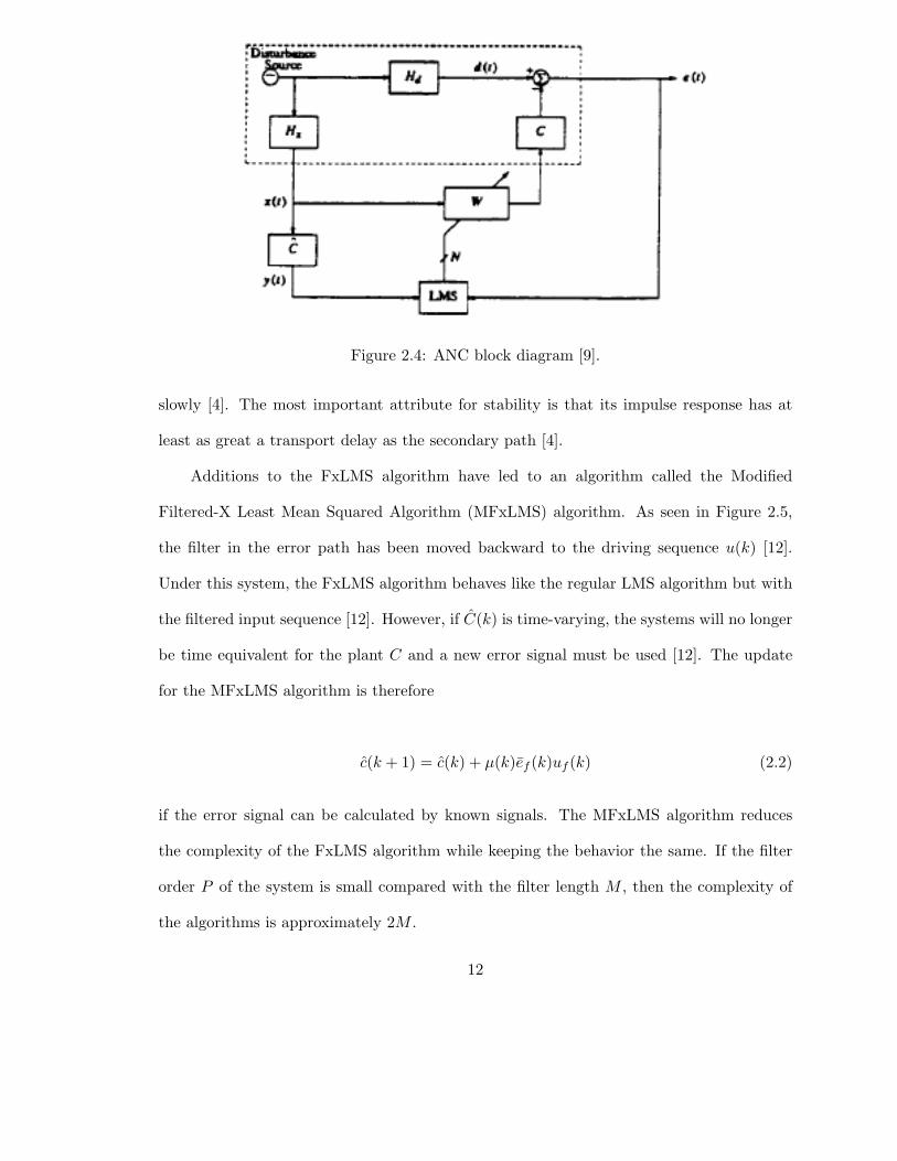
Figure 2.4: ANC block diagram [9].

slowly [4]. The most important attribute for stability is that its impulse response has at

least as great a transport delay as the secondary path [4].

Additions to the FxLMS algorithm have led to an algorithm called the Modified

Filtered-X Least Mean Squared Algorithm (MFxLMS) algorithm. As seen in Figure 2.5,

the filter in the error path has been moved backward to the driving sequence u(k) [12].

Under this system, the FxLMS algorithm behaves like the regular LMS algorithm but with

the filtered input sequence [12]. However, if C(k) is time-varying, the systems will no longer

be time equivalent for the plant C and a new error signal must be used [12]. The update

for the MFxLMS algorithm is therefore

c(k + 1) = c(k) + µ(k)ef (k)uf (k) (2.2)

if the error signal can be calculated by known signals. The MFxLMS algorithm reduces

the complexity of the FxLMS algorithm while keeping the behavior the same. If the filter

order P of the system is small compared with the filter length M , then the complexity of

the algorithms is approximately 2M .

12

Figure 2.5: Modified filtered-X LMS block diagram [12].

2.3.2 Infinite Impulse Response

Infinite impulse response filters are more common in describing the vibration response

of structures in active structural acoustic control due to the lightly damped quality of the

structures but have still found application in ANC [3]. The recursive least squares (RLS)

algorithm can quickly model the response of the system without the need for feedback

cancellation [4]. However, unlike the FIR FxLMS filter described in the previous section,

the RLS algorithm has a greater possibility of instability as an IIR filter. Extensions

of stable RLS algorithms, such as the inverse QR-RLS algorithm (IQR-RLS) and the QR

decomposition least-squares-lattice (QRD-LSL) have been developed [15]. These algorithms

are combined with the modified version of the FxLMS algorithm whose delay-compensating

structure eliminates the need to reduce the adaptive gain in the update equation of the

adaptive filters because of the delay found in the error path between the actuators and

the error sensors [15]. The modified version of the FxLMS structure, as it pertains to the

following description of the IQR-RLS algorithm, is shown in Fig. 2.6.

The IQR-RLS algorithm is used in broadband multichannel ANC systems and must

explicitly compute the time domain coefficients of the filters [15]. The block delay line

structure is a requirement for fast versions of the RLS algorithms [15]. This block delay line

13

Figure 2.6: Modified filtered-X structure for RLS [12].

structure arises from the transform of the values of the filtered reference signal, V (n) [15].

The samples in V (n) are the samples of V (n−1) that have been delayed by one sample except

for the first block of samples (the new samples) in V (n) and the last block of samples in

V (n−1) which are discarded [15]. The equations for the IQR-RLS algorithm are as follows:

yj(n) =I∑

i=1

wTi,j(n)xi(n) (2.3)

vi,j,k(n) = hTj,kx

,i(n) (2.4)

dk(n) = ek(n) −J∑

j=k

hTj,kyj(n) (2.5)

e′

k(n) = d′

k(n) +I∑

i=1

J∑

j=1

wTi,j(n)vi,j,k(n) (2.6)

14

The computational load for the IQR-RLS algorithm for multichannel ANC systems

has a computational load proportional to (IJL)2 [15]. Therefore, the computational load

increases with L2 [15].

The QR decomposition least-squares-lattice (QRD-LSL) algorithm improves on the

IQR-RLS algorithm by increasing the computational load by only L while still maintain-

ing numerical stability [15]. However, it cannot provide the time-domain adaptive filters

coefficients needed for the upper path of the ANC structure shown in Fig. 2.6 [15]. To com-

pensate, the inverse transformation is required, but again, the computational load would

approach (IJL)2 [15]. As long as the period between updates is less than the time con-

stant caused by the forgetting factor λ, common to all LMS algorithms, the convergence

performance is not affected greatly [15]. Although the QRD-LSL algorithm requires less

computations, the IQR-RLS algorithm is simpler to implement and can be more stable if

low precision numerical representations(12 or 16 bits fixed point) or ill-conditioned systems

(more actuators than error sensors) are used [15]. Both the QRD-LSL and the IQR-RLS

algorithms are stable in 32 bit floating point environment.

Another IIR filter that uses the lattice structure is the gradient lattice algorithm (GL).

Like all IIR filters, the GL algorithm is not unconditionally stable due to the possibility that

some poles of the filters will move outside of the unit circle during the weights update [6].

Also, most IIR adaptive algorithms have a lower convergence speed and may converge to a

local minimum [6]. The lattice structure for the GL algorithm possesses the advantage of

inherent stability and greatly reduced sensitivity to the eigenvalue spread of the reference

signal [6]. The GL algorithm makes full use of the orthogonalization property of the lattice

structure and avoids the problem of slow convergence and possible instability while holding

the benefits of an adaptive IIR filter [6].

15

Figure 2.7: Gradient lattice block diagram [6].

M additional lattice filters are needed to obtain the filtered regressor signals −∆Θk(n)

corresponding to the rotation parameters [6]. These filtered regressor signals are formed by

filtering the input with the cancellation path transfer function and the lattice filter and can

be obtained with an auxiliary lattice filter [6]. Since M additional lattice filters are needed,

the complexity of the system is of the order M2 for computation as well as storage [6].

Among IIR filters, this additional complexity is a disadvantage. However, by simplifying

the computations, a gradient lattice algorithm can be obtained that is of order M [6]. The

resulting algorithm is as follows [6]:

vk(n + 1) = vk(n) − µe(n)Bk(z)C(z)x(n), k = 0, 1, ..., M (2.7)

Θk(n + 1) = Θk(n) + µe(n)γkzBk−1(z)W (z)x(n), k = 1, 2, ..., M (2.8)

The GL algorithm’s performance can be measured with the commonly used adaptive

IIR filters, the filtered-u LMS (FULMS) algorithm and the filtered-v LMS (FVLMS) algo-

rithms, both of which suffer from instability and slow convergence. Compared with these

direct form IIR filters, the convergence for the GL algorithm should be about the same for

16

Figure 2.8: Convergence comparison between (a)GL, (b) FULMS, and (c) FVLMS algo-rithms [6].

a noise signal with a flat power spectrum, but since lattice form adaptive IIR filters are

more stable, the convergence coefficient can be set larger to achieve a faster convergence

speed [6]. As seen in Fig. 2.8, the comparison between the GL algorithm and other IIR

algorithms shows that the GL algorithm converges faster and to a smaller mean squared

error [6]. It is also far less sensitive to the cancellation path modeling error [6].

2.4 Limitations of Active Noise Control

Active noise control is not appropriate for high frequency cancellation, as seen in

Fig. 2.9 from the consumer headset, Bose QuietComfort 2 ANC headphone. The spatial

character of a sound field depends on wavelength and as such, frequency [11]. Destructive

interference used by ANC is most efficient when the two sound fields can be aligned in space

over an acoustic wavelength [3]. These low frequency sounds have wavelengths that are large

compared to the zone in which the noise is canceled and are therefore more conducive to

ANC than high frequency sounds [3]. For example, a sound wave with a frequency of 100

Hz, will have a wavelength of about 3.4 meters under normal conditions [4]. Sounds at

17

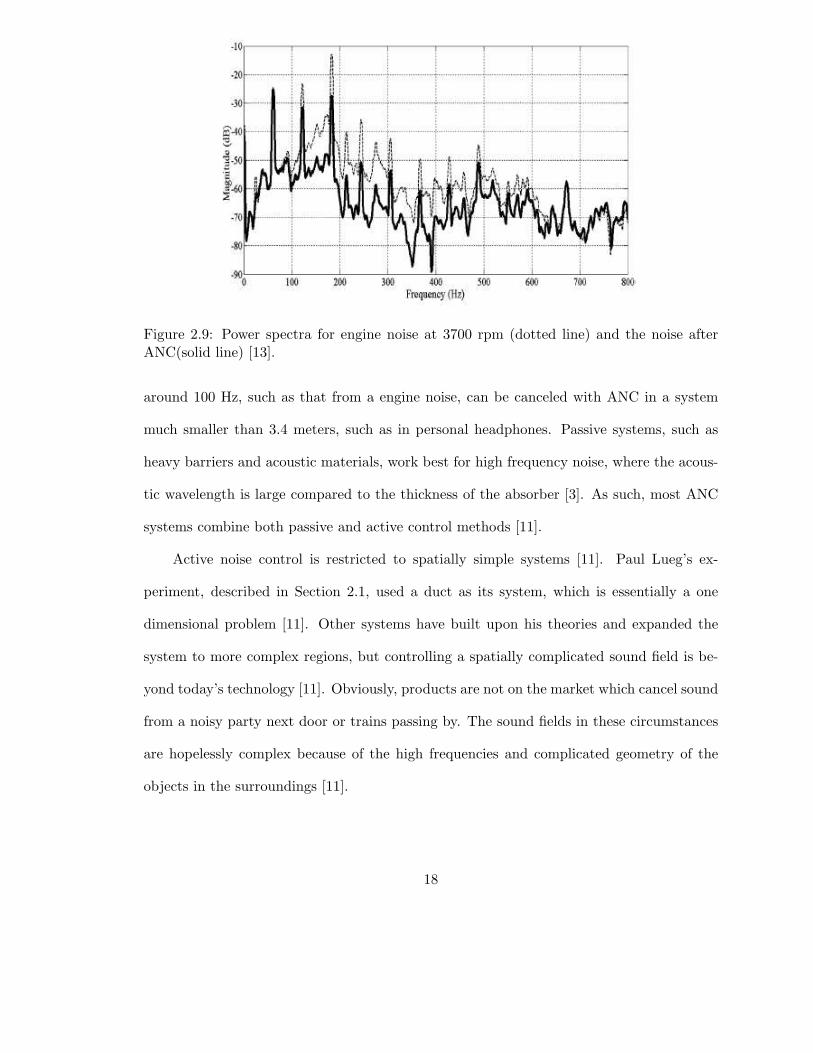
Figure 2.9: Power spectra for engine noise at 3700 rpm (dotted line) and the noise afterANC(solid line) [13].

around 100 Hz, such as that from a engine noise, can be canceled with ANC in a system

much smaller than 3.4 meters, such as in personal headphones. Passive systems, such as

heavy barriers and acoustic materials, work best for high frequency noise, where the acous-

tic wavelength is large compared to the thickness of the absorber [3]. As such, most ANC

systems combine both passive and active control methods [11].

Active noise control is restricted to spatially simple systems [11]. Paul Lueg’s ex-

periment, described in Section 2.1, used a duct as its system, which is essentially a one

dimensional problem [11]. Other systems have built upon his theories and expanded the

system to more complex regions, but controlling a spatially complicated sound field is be-

yond today’s technology [11]. Obviously, products are not on the market which cancel sound

from a noisy party next door or trains passing by. The sound fields in these circumstances

are hopelessly complex because of the high frequencies and complicated geometry of the

objects in the surroundings [11].

18

Canceling sound in enclosed spaces at low frequencies, such as in a helicopter cockpit,

has been successful because the wavelength of the noise is similar or longer than the dimen-

sion of the enclosure [11]. The sound field in an enclosure is typically created by standing

waves and depends on the superposition of a number of acoustic modes [3]. These modes

are characterized by the number of wavelengths that fit along one dimension of the enclo-

sure [3]. Depending on the geometry of the enclosure, the mode will have a corresponding

natural frequency. At an excitation frequency larger than this natural frequency, the sec-

ondary source will be unable to reduce the acoustic energy in the enclosure due to natural

frequencies from other acoustic modes [3]. The natural frequencies from the other acoustic

modes prevent the secondary source from reducing the amplitude of one mode without re-

ducing the amplitude of at least one of the other modes [3]. Multiple secondary sources are

then needed to control every mode [3]. When the number of acoustic modes contributing

to the total energy at one frequency increases dramatically with excitation frequency, the

modal overlap increases in proportion to the cube of the excitation frequency [3]. Doubling

the upper frequency of active control requires eight times the number of loudspeakers at

the original frequency [3]. It follows that broadband noise is much harder to cancel than

narrowband or a single tone and harmonics [11]. Also, lightly damped systems are easier

to control than heavily damped systems [11].

In wide open spaces, however, the reduction of sound in one localized region can actually

amplify noise in another region [11]. Two components of sound pressure in phase will create

constructive interference and actually increase the sound level [4]. Global noise cancellation

only occurs for simple sound fields where impedance coupling is the primary mechanism [11].

Like enclosed spaces, more actuators are needed for complex sound fields to obtain global

reductions, and higher frequencies complicate sound fields to the point that hundreds of

actuators are needed for global control [11]. On the other hand, directional cancellation is

19

possible at fairly high frequencies if the actuators and control system can accurately match

the phase of the disturbance [11].

The control method used to cancel sound has a significant impact on how well ANC

works for a system. If a disturbance can be measured before it reaches the region where

sound attenuation is desired, feedforward control can be used to measure the actuator

signal [11]. If not, then feedback control must be used to compute the actuator signal

solely from error measurements [11]. For example, random noise in an aircraft due to air

turbulence has no single observable source for an external reference signal in feedforward

control [3]. Feedback control must be used in this situation. Under most conditions, how-

ever, feedback control is less stable than feedforward control and tends to be less effective

at high frequencies [11]. The bandwidth over which attenuation is achieved is limited by

the delay in the plant [3]. Since the bandwidth is proportional to the delay in seconds, the

phase shift associated with the delay changes the sign of the feedback at higher frequencies,

which results in a positive feedback system and more sound [3]. Therefore, the microphone

must be close to the loudspeaker in order to reduce the acoustic propagation delay [3].

2.5 Commercial Products

Although ANC systems have shown in successful demonstrations to cancel noise, its

applications are few [11]. A few applications that have been successful include canceling

noise in enclosed spaces such as ducts, vehicle cabins, exhaust pipes, and headphones [11].

2.5.1 ANC Headphones

Noise canceling headphones are the most successful consumer product that uses ANC.

These headphones cancel noise in the environment while allowing the user to listen to

music. As seen in Fig. 2.10, the system consists of earmuffs containing speakers and one

20

Figure 2.10: Noise canceling headphone using ANC [3].

or more small circuit boards [11]. Like most ANC commercial products, ANC headphones

take advantage of an enclosure to carry out ANC. The microphone can be placed within

one centimeter of the loudspeaker, thus reducing the propagation delay and enabling the

feedback controller to cancel frequencies of about 1 kHz [3]. Additionally, the proximity

to the ear canal provides a favorable acoustic environment in which the attenuation of

the sound pressure at the microphone results in similar attenuation of the ear [3]. As of

this writing, active control headsets are available for relatively cheap prices in standard

electronics stores across the United States.

The two control systems for ANC, feedforward and feedback control, have both been

implemented in ANC. Feedforward control, while the focus of research in communication

and entertainment headsets, has significant stability and performance problems caused by

nonstationary reference inputs, measurement noise, and acoustic feedback [5]. In feedfor-

ward control, the reference input is placed outside of the ear cup to pick up the primary

noise x(n) [13]. The reference signal x(n) is processed by the ANC system to generate

21

Figure 2.11: Locations for an error microphone for ANC headphones [13].

the control signal y(n) to drive a secondary loudspeaker inside the ear cup for producing

antinoise [13]. The FxLMS algorithm minimizes the residual noise e(n), which is in turn

measured by the error microphone [13]. The ideal location of the error microphone occurs

where the frequency response of the system is flattest with the least number of dips and

peaks [13]. This location is found experimentally in [13] to be near the external auditory

meatus of the ear, which allows the microphone to be placed in the hollow in that location

at location 8 of Fig. 2.11.

The secondary path S(z) includes the digital-to-analog converter, reconstruction filter,

power amplifier, loudspeaker, acoustic path from loudspeaker to error microphone, error mi-

crophone, preamplifier, antialiasing filter, and analog-to-digital converter [13]. The FxLMS

algorithm places the secondary path estimate in the reference signal path to the weight

update of the algorithm [13]. This model is usually estimated using white noise as the exci-

tation signal, but for headphone applications, the white noise can be irritating [13]. In [13],

music has been shown to perform as well as white and chirp noise for the excitation signal.

22

Figure 2.12: Integrated audio and ANC system block diagram [5].

Feedback control, however, provides more accurate noise cancellation since the micro-

phone is inside the ear cup of the headset [5]. Specifically, the FxLMS algorithm, described

in Section 2.4.1, is used in [5] to achieve a complete adaptive feedback ANC system. To-

gether with the FxLMS system, the desired audio input can be integrated to form the in-

tegrated feedback active noise control (IFBANC) system [5]. This system uses the residual

noise picked up by the error microphone to synthesize the primary noise x(n) for updating

the adaptive filter coefficients using the FxLMS algorithm [5]. The IFBANC is integrated

with the existing audio playback system or communication headset to pick up both the

residual noise and the desired audio signal as seen in Fig. 2.10 [5].

Figure 2.12 shows the block diagram of the combined audio and ANC system. The error

sensor output signal, e(n), contains both the residual noise and the desired audio signal [5].

The audio components in e(n) are then removed by the audio interference cancellation filter

S(z) using the audio signal a(n) as the reference signal [5]. The adaptive noise control filter

W (z) is updated with the difference error signal e′(n) which consists of the residual noise [5].

23

The optimal solution for the audio interference cancellation filter is

E′(z) = D(z) − Y (z)S(z) (2.9)

which shows that the E′(z) is reduced to the residual error of the ANC system where the

primary noise D(z) is canceled by the anti-noise Y (z)S(z) [5].

Several advantages of the IFBANC system become apparent. First, the true residual

noise e′(n) can be estimated well without interfering with the audio signal a(n) [5]. Second,

a large step size can be used in adapting the cancellation filter W (z) since the difference

error signal e′(n) used by the FxLMS algorithm is not corrupted by the high volume audio

signal [5]. As stated earlier, the adaptive feedback ANC technique allows for more accurate

noise cancellation since the microphone is placed inside the ear muff [5]. The system creates

a cheap, compact, lower power consumption solution [5]. Finally, the audio signal can be

used to drive the modeling of the secondary path transfer function [5].

Figure 2.13 shows the noise spectrum comparison between an ANC and non-ANC

system undergoing a disturbance from a siren alternating between 775Hz and 965Hz [5].

The reduction in noise at the peaks is easily observed. The noise reduction by the IFBANC

system is more than 40 dB and 30 dB at 775Hz and 965Hz, respectively [5]. Fig. 2.13 shows

the spectrum for a disturbance of engine noise from a welding power generator at 3700

rpm [5]. The narrowband harmonics at 61Hz, 122Hz, and 183Hz, were canceled by more

than 30 dB. These results show that ANC headphones can significantly reduce noise from

industrial sources [5].

2.5.2 Other Products

Industries have used ANC on a limited basis in creating more efficient system compo-

nents. Active mufflers for industrial engine exhaust stacks, commercial compressors, and

24

Figure 2.13: Noise spectrum comparison for ANC and non-ANC systems from siren distur-bance [5].

generators reduce the noise output of these components [11]. Even automobile manufac-

turers are looking into ANC for active mufflers, although there are no current production

automobiles with active mufflers available [11]. Industries have used ANC for their large

industrial fans to reduce low-frequency noise downstream and upstream [11]. These ANC

systems improve efficiency to such an extent that they pay for themselves within a year or

two [11].

Adaptive feedforward controllers have been used to control the low-frequency engine

noise in automobiles and cabin noise in propeller aircraft such as helicopters and air-

planes [3]. Despite many successful demonstrations of ANC systems for both low frequency

engine and road noise, fully active control systems are currently fitted to very few produc-

tion vehicles [3]. At least one automobile in Japan offers ANC as a factory option [11].

25

Figure 2.14: Noise spectrum comparison for ANC and non-ANC Systems from engine dis-turbance [5].

Most systems for automobiles involve superposing cancellation signals over the regular mu-

sic signals in car stereo speakers to cancel muffler noise and engine noise [3]. However, these

systems are expensive and not at all common [11].

In passenger propeller aircraft, ANC systems have been embedded inside the walls to

cancel the propeller noise [3]. They primarily use rare-earth magnets to reduce their weight

and generate high sound pressure levels at low frequencies to match that of the propeller

noise [3]. Although this high sound pressure is not heard from cancellation, any high

frequency components due to loudspeaker distortion will be clearly audible [3]. High quality

components are used to reduce the likelihood of this happening [3]. A system made by Ultra

Electronics, Cambridge, England for the Saab 2000 aircraft uses 37 loudspeakers and 72

microphones [3]. Ultra and Lord Corporation uses eight loudspeakers and 16 microphones in

26

their ANC system for the smaller Beechcraft King Air aircraft [3]. The primary advantage

to these systems is dramatic weight savings compared with using only passive systems [11].

27

Chapter 3

Active Voice Control

3.1 Differences between Active Noise Control and Active Voice Control

Active voice control (AVC) uses the strategies of ANC to cancel unwanted speech. The

disturbance source of the AVC system is the voice of a speaker whose voice is to be canceled.

The actuators and sensors, like in ANC, are distributed in the environment. The antinoise

created by the adaptive filters is broadcast by the actuators to cancel speech. The purpose

of canceling speech is not to reduce the volume of the sound like ANC does for noise since

people do not normally speak or even shout at dangerous hearing levels. Instead, AVC

cancels speech to prevent unwanted communication and annoying speech. Because of this,

the antinoise of the sound does not need to be as loud as that for a system canceling sound

in an industrial fan.

The properties of speech itself are different from the regular noise canceled by ANC

systems. ANC systems usually cancel noise with frequency components under 500Hz. The

speech frequency range, however, spans from about 80Hz to 3500Hz. There is a 420Hz

overlay between ANC and AVC, which limits the number of people whose voice is affected

by AVC. The noise canceled using ANC is usually periodic in nature like that from a

propeller or from a duct. Human speech, however, can be thought of as random noise since

there is no way to predict what someone will say in the near future. The speech that must

be canceled in AVC is higher and wider in frequency as well as more random than noise

that is canceled by ANC.

28

Depending on the application, however, the spatial arrangement of these actuators and

sensors must compensate for the mobility of people. In ANC, the actuators and sensor

locations are placed in set locations relative to the disturbance source, such as the walls of

an airplane to cancel the propeller noise of the aircraft. In those circumstances, the sound

fields, whose inherent variability is compensated by the adaptive filters, will not move away

from the noise from the propellers for an ANC system. The speaker, however, can move

between many different environments. The actuators and sensors, at least in an open air

environment, will need to be placed with the speaker, or the speaker must stay in one

location in order for their speech to be canceled.

The approach for the environment type (open or enclosed) for AVC differs from that

of ANC. ANC can eliminate noise in enclosed spaces using multiple sensors and actuators.

The use of AVC in enclosed spaces, however, is limited since the application of many sensors

and actuators to cancel the speech of one person will not be viable for multiple people or

for an enclosure where people commonly move in and out.

3.2 Difficulties with Voice Control

As mentioned before, vocal frequencies are higher than the noise canceled by ANC.

The upper frequency limit of ANC is set by the size of the wavelengths in the noise. For

vocal ranges, the wavelengths are much smaller than the corresponding wavelengths at low

frequencies, and the space at which the high frequency sounds are canceled becomes too

small for practical applications. The range of 420Hz at which the operating frequency range

of ANC will work with speech is too small to reasonably suggest as a true implementation

of AVC for all voice pitches. Typical strategies of ANC will cancel the fundamental tones of

a typical male at 88-145Hz [1]. Nevertheless, the brain will create the missing fundamental

29

using the harmonics of the voice, thereby masking the cancellation [10]. Therefore, the

harmonics of the speech must be canceled as well.

The arrangement of actuators and sensors are dependent on the sound field properties

of the system. For AVC, the speaker can move between many different environments. The

components of AVC must therefore be on the speaker as he moves between environments,

or the speaker must stay in the area of voice cancellation. These two options are naturally

application dependent. The more complex of these strategies is the mobile AVC user mov-

ing between different environments. The antinoise from the actuators in this strategy must

compensate for differences in the environment. As such, a multiple sensor and actuator

arrangement similar to ANC is not viable due to its reliance on positioning in the envi-

ronment itself. Instead, a multiple sensor and actuator arrangement may be successful if

placed at various points on the speaker himself to achieve a full measurement of the sound

field of the surrounding system. The strategy involving the user staying in a predetermined

area of voice cancellation poses problems as well. In ANC systems using multiple sensor

and actuators in the environment, the region for cancellation is generally in an enclosure

where the sensors and actuators are spaced to suit the noise to be canceled. The voices for

different people can require separate geometries for these sensors and actuators, making a

generic arrangement of sensors and actuators impossible to build. Also, since the area of

cancellation is an enclosure anyway, passive sound control will cancel speech like that of a

speaker in a telephone booth mentioned in the previous section.

For just one actuator and sensor, the region for cancellation can be in both an open

air environment or an enclosed environment. In an enclosed environment, the frequency

range is limited to low frequencies as it is in ANC. For the open air environment, the

cancellation can be expected to act similar to that presented in the Single Sensor and

Actuator Scheme section above. When the disturbance reaches the secondary source and

30

Figure 3.1: Overhead view of the preservation of speech due to the wake of silence.

antinoise, the unwanted voice attenuates in a wake of silence away from the source of the

disturbance, as shown in Fig. 3.1. This region provides the system with the directional

cancellation to cancel the voice from people nearby. The wake in current systems is small

due to the high frequencies involved. The technology must be improved before the open air

environment can be adequately used to cancel high frequency sounds.

Control for AVC systems will generally be regarded as feedback since the disturbance

can not be measured before it reaches the region for sound attenuation. The adaptive

filters, then, must rely solely on the feedback signal to calculate the antinoise of the system.

Unfortunately, feedback control tends to be less stable and less effective at high frequencies,

which is certainly necessary for voice attenuation.

The act of silencing a person’s speech can extend into ethical issues as well. The basic

freedom of speech can be broken by the use of AVC to cancel speech. Certainly, AVC

should not be used as a means of silencing critics or keeping people from communicating

with one another. Therefore, the user of AVC, who desires their own speech canceled,

should be the only one whose voice is canceled to prevent communication. A situation in

which the user destructively cancels the voice of a colleague or opponent is not ethically

sound. Alternatively, AVC can be used to cancel residual speech as long as the AVC only

31

cancels the voice in the immediate surroundings where the speech is undesired. The source

of the speech should not be affected by AVC or perhaps even realize that their voice is being

canceled. An example of this is speech between cubicles in an office environment. AVC can

be employed from one cubicle to cancel the conversation from another cubicle as long as the

two speakers can still communicate. Note that this is completely different to noise masking,

where sound is played to drown out the noise of other people’s speech and does not employ

sound control.

The situation of canceling the user’s speech creates another problem with using AVC

- when would a user need their own voice canceled but still feel the need to speak? One

application, elaborated in Section 3.3.1, uses a cell phone to speak to someone over the

phone while canceling his speech to possible listeners. In all applications, the speech of the

user would have to be preserved before being canceled in order for the user to communicate

effectively but still prevent those in the surrounding environment from hearing the speech.

The result of this is a vicious circle between preserving and canceling the speech. The voice

coming from the mouth is canceled in the air, which results in no sound. At the same time,

the voice from the air is picked up by the cell phone for communication to the listener on

the other end. Naturally, the desired listener and the unwanted listener must be isolated

from each other and must receive separate sounds.

Two possible resolutions occur for this contradiction. ANC itself never completely

eliminates the noise. Instead, it generally reduces the sound from dangerous to safer levels

by less than 100dB. The performance of AVC can be expected to match that of ANC given

an idealized circumstance where AVC works as well as ANC. The attenuated voice, then,

can be picked up by the cell phone for transmission. The other solution to the contradiction

of preservation of voice to its cancellation is using the wall of silence between the boundaries

of the region of suppressed voice and the region of the source of the voice. As given in [14],

32

the region of silence after the secondary canceling source actually acts like a wake moving

away from the disturbance source. This wake can act as directional cancellation away from

the AVC user. The speech signal can then be picked up before it reaches the wall of sound

and the resulting wave. Unfortunately, since AVC uses ANC methods, the wake will be

very small due to the high frequency components of the speech signal [14].

3.3 Applications

3.3.1 Mobile Cellular Phone Booth

The mobile cellular phone booth is a theoretical application which uses AVC to cancel

the voice of the speaker on a cell phone while preserving the speech itself for the recipient

on the other end of the cell phone. The mobile cellular phone booth does not use the

passive systems of typical telephone booths to attenuate noise. Instead, the AVC eliminates

the sound in the surrounding environment. The benefits of this system are privacy for

the speaker and for those people around the speaker, not having to listen to a one way

conversation. The components of the system include a digital signal processing (DSP)

microchip in the cell phone and the secondary speaker which is very close to the input

microphone to reduce the delay in the plant. This delay actually limits the bandwidth of

cancellation, so reducing the distance from the microphone and secondary source will help

increase the upper bound of frequency for control. The microphone of the cell phone acts as

both the receiving microphone for capturing the speech for the user on the other end of the

cell phone, and as the error microphone for the adaptive filter for the DSP microchip. When

the user speaks, his voice is picked up by the microphone and sent through the network

to the listener on the other end of the line. At the same time, the speech signal is sent

into the DSP microchip, which in turn creates the antinoise of the system. This antinoise

then attenuates the speech. The control system for this type of system must be feedback

33

due to the lack of a reference signal with which to better approximate the antinoise for a

feedforward system. The attenuated noise can again be picked up by the system, broadcast

to the other end, and used to drive the DSP chip. The attenuation of the speech occurs in

a wake following the secondary source, which provides a somewhat directional trait to the

layout of the cancellation. If necessary, additional secondary sources can be added to the

cellular phone to provide cancellation in even more directions.

The mobile cellular phone booth can only exist as a theoretical application with today’s

technology. As with basic AVC itself, the frequency of voice is too high for ANC algorithms

to work correctly. Also, the geometry of a constantly changing system is too complex for

a single microphone to adequately cancel the voice, even if the voice could be attenuated

thoroughly. Additional microphones are not feasible since they would not provide a complete

understanding of the system. These additional microphones must be on the person instead

of in the environment. As stated earlier, cancellation systems are restricted to spatially

simple systems. Especially in open air environments, ANC and AVC can create constructive

interference and actually amplify the disturbance noise in certain locations of the sound field.

This constructive interference can be attributed to the path between the antinoise and the

distance traveled away from the disturbance. The additional volume in the speech from

the constructive interference will result in even more annoyance to other listeners than the

regular speech on the cell phone and possibly amplify the speaker’s speech that was thought

to be private.

3.3.2 Residual Voice Cancellation

Residual voice cancellation (RVC) uses AVC to cancel voice without infringing on

the wanted communication of the original speaker. One exception to using AVC in an

enclosure that employs RVC is in a telephone booth. In this system, the residual voice

34

is that speech that is heard outside of the telephone booth. This speech is not desired

for both the observers outside of the telephone booth as well as the speaker, who may

want his conversation kept confidential. The walls of the telephone booth act as its passive

cancellation and cancels sound above 1000Hz. The addition of AVC in the telephone booth

reduces the sound levels heard by outside observers by reducing the frequency range below

500Hz. The performance of the telephone booth in canceling sound in the mid-range, or

500Hz-1000Hz, is enhanced. Additionally, since the walls of the telephone are outside of

the mouth for voice and the microphone for the telephone, only the AVC system will affect

the voice volume levels going into the receiver of the telephone. Telephones employ usable

frequency ranges from 300Hz to 3400Hz, which preserves enough harmonics for a discernible

pitch of the voice by the listener on the other side of the telephone line. As such, only the

lower frequency components of the voice will be canceled, and the observer outside of the

telephone booth will hear reduced sound levels over all frequency ranges. However, AVC

for this application is merely ANC under another name that cancels voice.

Another application for RVC which is much more difficult to implement is cancellation

of voice in an open air environment such as the cubicle speech mentioned in Section 3.2. In

this situation, the user of AVC wants to cancel the voices of the conversation in a nearby

cubicle only in the immediate area so as not to cancel the conversation speech itself. Like

the mobile cell phone booth, AVC must be able to reduce the entire frequency range of

human speech to account for all ranges of voice. It must also account for any geometry of

the surrounding objects and the resulting complex sound fields from the presence of those

objects. ANC, and therefore AVC, is unable to complete either of these tasks, making the

mobile cell phone booth and the RVC for the cubicle impossible with today’s technology.

35

Chapter 4

Simulation

A simulation using MATLAB’s Simulink was conducted to determine the validity of

AVC by applying ANC with voice. The first experiment determined if a sinusoid at mid-

range for voice frequencies could be canceled by inverting the sinusoid by 180 degrees.

In Fig. 4.1, one sinusoidal source produces a frequency of 1710Hz, while the other source

produces a sinusoid with a frequency of 1710Hz but at π radians out of phase. The speaker

while the simulation is running produces no sound. As expected, this simulation proves

that the principles of sound control work with vocal range sounds. The superposition of

the two signals at opposite phase cancels both signals.

4.1 The Active Sound Control Simulink Diagram

Applying the current ANC strategies to cancel sound involves more than just adding

two sound waves. As explained above, various adaptive filters are used to adjust for a

dynamic plant to create the antinoise of the system. Using the adaptive filter tutorials from

the Signal Processing Blockset on the MathWorks website [8], an acoustic environment and

an ANC system was modified to implement AVC. The acoustic environment creates two

signals - the original signal representing the vocal sound and the noisy signal representing

the vocal sound after filtering and the desired output. These two signals are used by the

AVC system as the inputs to the normalized LMS (NLMS) algorithm, where the original

signal is the desired output of the NLMS algorithm and the filtered vocal and desired output

is the input of the NLMS algorithm. The error output represents the resulting sound of

36

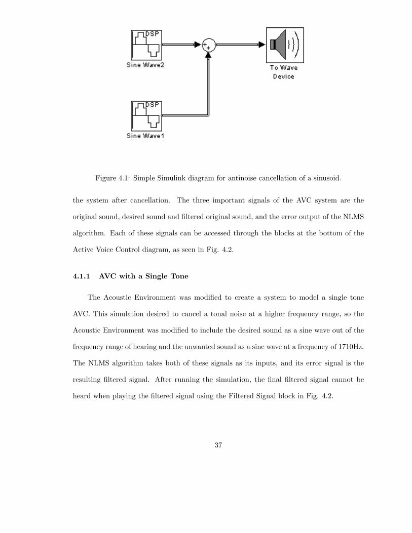
Figure 4.1: Simple Simulink diagram for antinoise cancellation of a sinusoid.

the system after cancellation. The three important signals of the AVC system are the

original sound, desired sound and filtered original sound, and the error output of the NLMS

algorithm. Each of these signals can be accessed through the blocks at the bottom of the

Active Voice Control diagram, as seen in Fig. 4.2.

4.1.1 AVC with a Single Tone

The Acoustic Environment was modified to create a system to model a single tone

AVC. This simulation desired to cancel a tonal noise at a higher frequency range, so the

Acoustic Environment was modified to include the desired sound as a sine wave out of the

frequency range of hearing and the unwanted sound as a sine wave at a frequency of 1710Hz.

The NLMS algorithm takes both of these signals as its inputs, and its error signal is the

resulting filtered signal. After running the simulation, the final filtered signal cannot be

heard when playing the filtered signal using the Filtered Signal block in Fig. 4.2.

37

Figure 4.2: Active voice control Simulink diagram for single tone cancellation.

4.1.2 AVC with Recorded Speech

To better approximate the performance of the simulation, the Acoustic Environment

was modified further to record speech from a microphone which is then played back as the

filtered sound after the simulation is over. As seen in Fig. 4.5, the setup closely approximates

that of the single tone simulation but with microphone inputs instead of sinusoid sources.

As the simulation is running, the user speaks into a microphone. The signal from the

microphone becomes the disturbance for the AVC system. The desired signal is set at 15kHz.

The desired signal will effectively push the frequency of the disturbance to higher frequencies

to reduce the sound. The filtered signal after the simulation has ended is attenuation of

the speech. These results were found to vary among many people who participated in the

simulation. Several stated that they could hear attenuation of their voice, while others

could not. The different frequencies of the participants’ voices as well as the complexity of

their voices probably contributed significantly to this variation in results.

38

Figure 4.3: Acoustic environment for single tone cancellation.

Figure 4.4: Active voice control Simulink diagram for recorded speech cancellation.

39

Figure 4.5: Acoustic environment Simulink diagram for recorded speech cancellation.

40

Chapter 5

Conclusion

The technology behind ANC must extend its range into higher frequencies before open

cancellation of complex frequencies and sound fields can be achievable. If this technology

is developed, cancellation of any type of sound will be possible, and passive techniques may

be quickly eliminated. Unfortunately, as stated in [3]:

. . . active noise control is restricted to relatively low frequency applications.

This is because it is only at such low frequencies that the acoustic wavelength is

large compared to the dimensions of the volume being controlled. Active control

will thus never become a universal solution for all acoustic noise problems.

Even though ANC can be applied to higher frequencies to cancel voice as shown in the

given simulations, the region of cancellation is too small for canceling a region large enough

for a practical implementation. Even if the region was large enough, experiments show

that ANC in open air environments can actually create more sound instead of canceling it.

Despite these setbacks, AVC may be applicable within the operable range of ANC. Future

work will be needed to take advantage of this potential area of research.

41

Bibliography

[1] R. Baken and R. F. Orlikoff, Clinical Measurement of Speech and Voice. Thomson DelmarLearning, 2nd edition, 2000.

[2] M. Bouchard, “New recursive-least-squares algorithms for nonlinear active control of soundand vibration using neural networks,” IEEE Transactions on Neural Networks, vol. 12, pp.135–147, 2001.

[3] S. Elliot, “Down with noise [active noise control],” IEEE Spectrum, vol. 36, pp. 54–61, 1999.

[4] S. Elliot and P. Nelson, “Active noise control,” IEEE Signal Processing Magazine, vol. 10, pp.12–35, 1993.

[5] W. S. Gan and S. Kuo, “An integrated audio and active noise control headsets,” IEEE Trans-

actions on Consumer Electronics, vol. 48, pp. 242–247, 2002.

[6] X. Q. Jing Lu and B. Xu, “A new adaptive iir algorithm for active noise control,” International

Conference on Acoustics, Speech, and Signal Processing, vol. 5, pp. 565–568, 2003.

[7] P. Lueg, “Process of silencing sound oscillations.” U.S. Patent No. 2043416, 1936.

[8] T. MathWorks, “Signal processing blockset: Adaptive filters.” Internet Tutorial, 2007. Avail-able from www.mathworks.com.

[9] D. Morgan and D. Quinlan, “Local silencing of room acoustic noise using broadband activenoise control,” in IEEE Workshop on Applications of Signal Processing to Audio and Acoustics,October 1993, pp. 23–25.

[10] e. a. Peter Schneider, “Structural and functional asymmetry of lateral heschl’s gyrus reflectspitch perception preference,” Nature Neuroscience, vol. 8, pp. 1241–1247, 2005.

[11] C. Ruckman, “Frequently asked questions: Active noise control.” Internet FAQ document,2007. Available via anonymous ftp from ftp://rtfm.mit.edu/pub/usenet/news.answers/, or viaUsenet in news:news.answers.

[12] M. Rupp, “Saving complexity of modified filtered-x-lms and delayed update lms algorithms,”IEEE Transactions on Circuits and Systems II: Analog and Digital Signal Processing, vol. 44,pp. 57–60, 1997.

[13] S. M. S.M. Kuo and G. Woon-Seng, “Active noise control system for headphone applications,”IEEE Transactions on Control Systems Technology, vol. 14, pp. 331–335, 2006.

[14] A. Wright and A. Karthikeyan, “Experimental characterization of the near field zones of silencein an active sound cancellation scheme,” in International Conference on Advanced Intelligent

Mechatronics, 1999.

[15] F. Yu and M. Bouchard, “Recursive least-squares algorithms with good numerical stability formultichannel active noise control,” International Conference on Acoustics, Speech, and Signal

Processing, vol. 5, pp. 3221–3224, 2001.

42

Appendix

The following figures are the Simulink diagrams for ANC from the adaptive filter tuto-

rial of the MathWorks website, found at [8]. Both of these diagrams were used in creating

the AVC Simulink diagrams presented in Chapter 4.

C or C++ code can be developed from all of the Simulink figures by generating them

from the Real-Time Workshop. This program is an addition to Simulink which allows

the user to generate code directly from the Simulink diagrams, thereby avoiding the code

writing stage of development. The Real-Time Workshop can generate code, an executable,

and html files after configuring the block diagram. Additionally, an option is available for

generating embedded programs on any microprocessor [8].

43

Figure 1: Acoustic Noise Cancellation Simulink Diagram [8]

Figure 2: Acoustic Environment Simulink Diagram for Active Noise Control [8]

44