BITS PilaniPilani Campus

EEE G529T PART 1 ANC LMS SINGLE TONE MATLAB

Vikas KalwaniEEE DepartmentBITS Pilani, Pilani

BITS Pilani, Pilani Campus

ACTIVE NOISE CONTROL

Why do we need Noise Control?

Noise control is a very important aspect of modern engineering systems

In aircrafts, control on the engine noise is a must for the Air Traffic Industry to Flourish

In the offices of MNC’s that work in the urban Residency amidst traffic and industrial

noises, Noise control is essential

Also, many biological problems due to Noise when uncontrolled

Types of Noise Control

ACTIVE PASSIVE

• Uses Active devices

• Efficient at low frequencies

• Selective Filtering

• Less Bulky

• Uses Passive elements like

Thermocol etc. to block the path of

the noise thereby attenuating it

BITS Pilani, Pilani Campus

BASICS

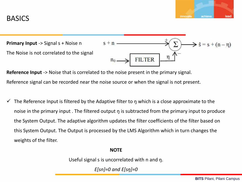
Primary Input -> Signal s + Noise n

The Noise is not correlated to the signal

Reference Input -> Noise that is correlated to the noise present in the primary signal.

Reference signal can be recorded near the noise source or when the signal is not present.

The Reference Input is filtered by the Adaptive filter to ŋ which is a close approximate to the

noise in the primary input . The filtered output ŋ is subtracted from the primary input to produce

the System Output. The adaptive algorithm updates the filter coefficients of the filter based on

this System Output. The Output is processed by the LMS Algorithm which in turn changes the

weights of the filter.

NOTE

Useful signal s is uncorrelated with n and ŋ.

E[sn]=0 and E[sŋ]=0

BITS Pilani, Pilani Campus

Subtracting noise from a signal involves the risk of distorting the signal and if done

improperly, may lead to increase in the noise level. So, the noise estimate ŋ should

be an exact copy of n

characteristics of the transmission paths are unknown and unpredictable, filtering

and subtraction are controlled by an adaptive process. Hence, an adaptive filter

capable of adjusting its impulse response to minimize an error signal (which

depends on the filter output) is used.

Error Signal/System Output is minimized using LMS, RLS, NLMS and other

algorithms

BITS Pilani, Pilani Campus

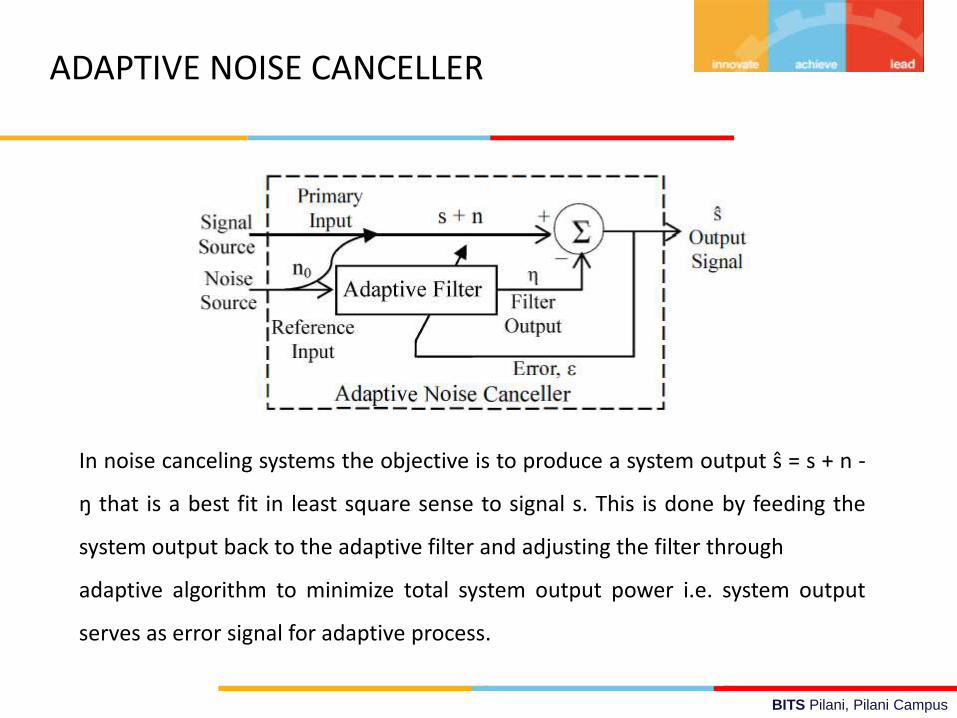
ADAPTIVE NOISE CANCELLER

In noise canceling systems the objective is to produce a system output ŝ = s + n -

ŋ that is a best fit in least square sense to signal s. This is done by feeding the

system output back to the adaptive filter and adjusting the filter through

adaptive algorithm to minimize total system output power i.e. system output

serves as error signal for adaptive process.

BITS Pilani, Pilani Campus

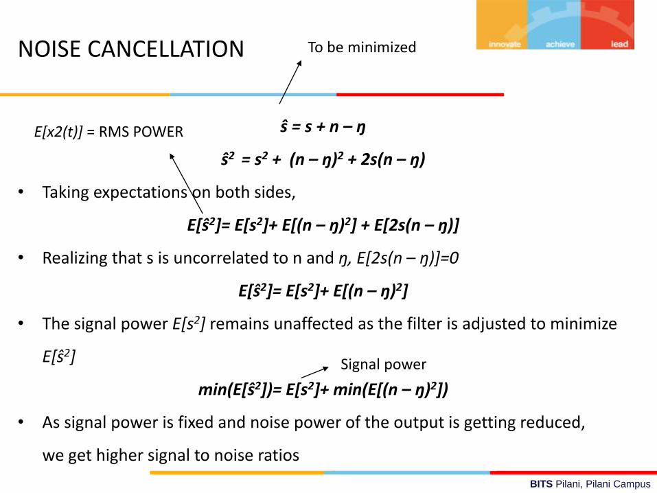
ŝ = s + n – ŋ

ŝ2 = s2 + (n – ŋ)2 + 2s(n – ŋ)

• Taking expectations on both sides,

E[ŝ2]= E[s2]+ E[(n – ŋ)2] + E[2s(n – ŋ)]

• Realizing that s is uncorrelated to n and ŋ, E[2s(n – ŋ)]=0

E[ŝ2]= E[s2]+ E[(n – ŋ)2]

• The signal power E[s2] remains unaffected as the filter is adjusted to minimize

E[ŝ2]

min(E[ŝ2])= E[s2]+ min(E[(n – ŋ)2])

• As signal power is fixed and noise power of the output is getting reduced,

we get higher signal to noise ratios

To be minimized

E[x2(t)] = RMS POWER

NOISE CANCELLATION

Signal power

BITS Pilani, Pilani Campus

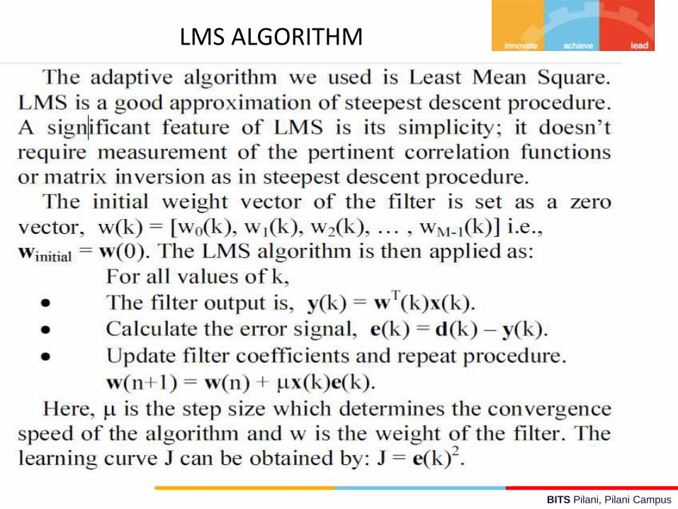
LMS ALGORITHM

BITS Pilani, Pilani Campus

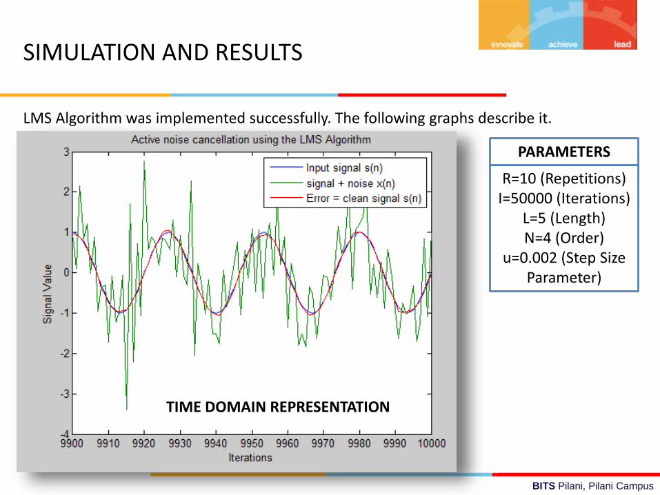
SIMULATION AND RESULTS

LMS Algorithm was implemented successfully. The following graphs describe it.

TIME DOMAIN REPRESENTATION

R=10 (Repetitions)I=50000 (Iterations)

L=5 (Length)N=4 (Order)

u=0.002 (Step Size Parameter)

PARAMETERS

BITS Pilani, Pilani Campus

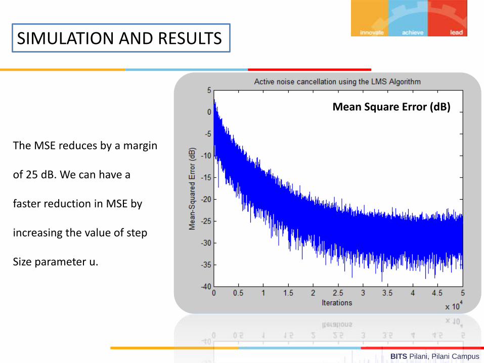
SIMULATION AND RESULTS

Mean Square Error (dB)

The MSE reduces by a margin

of 25 dB. We can have a

faster reduction in MSE by

increasing the value of step

Size parameter u.

BITS Pilani, Pilani Campus

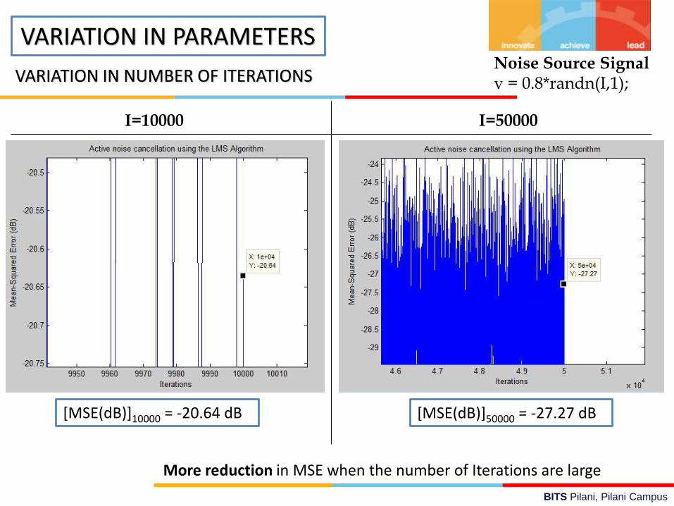
VARIATION IN PARAMETERS

VARIATION IN NUMBER OF ITERATIONS

I=10000 I=50000

Noise Source Signalv = 0.8*randn(I,1);

More reduction in MSE when the number of Iterations are large

[MSE(dB)]10000 = -20.64 dB [MSE(dB)]50000 = -27.27 dB

BITS Pilani, Pilani Campus

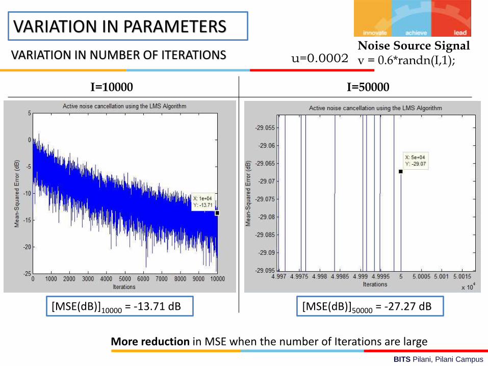
VARIATION IN PARAMETERS

VARIATION IN NUMBER OF ITERATIONS

I=10000 I=50000

Noise Source Signalv = 0.6*randn(I,1);

More reduction in MSE when the number of Iterations are large

[MSE(dB)]10000 = -13.71 dB [MSE(dB)]50000 = -27.27 dB

u=0.0002

BITS Pilani, Pilani Campus

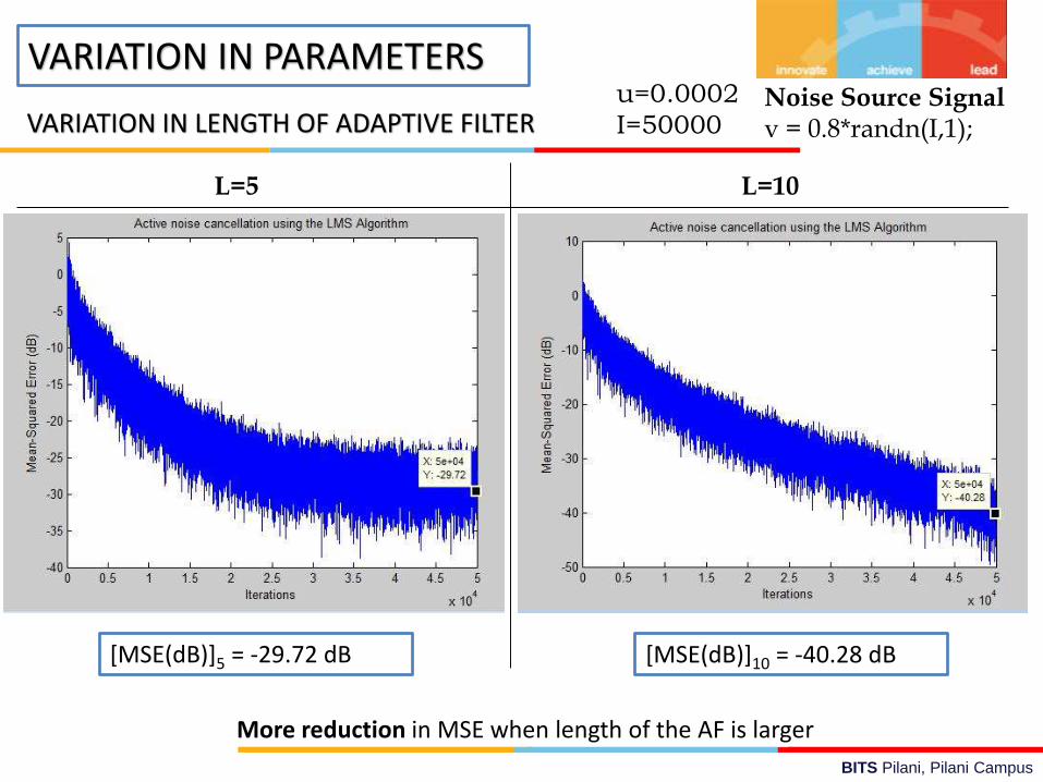
VARIATION IN PARAMETERS

VARIATION IN LENGTH OF ADAPTIVE FILTER

L=5 L=10

Noise Source Signalv = 0.8*randn(I,1);

More reduction in MSE when length of the AF is larger

[MSE(dB)]5 = -29.72 dB [MSE(dB)]10 = -40.28 dB

u=0.0002

I=50000

BITS Pilani, Pilani Campus

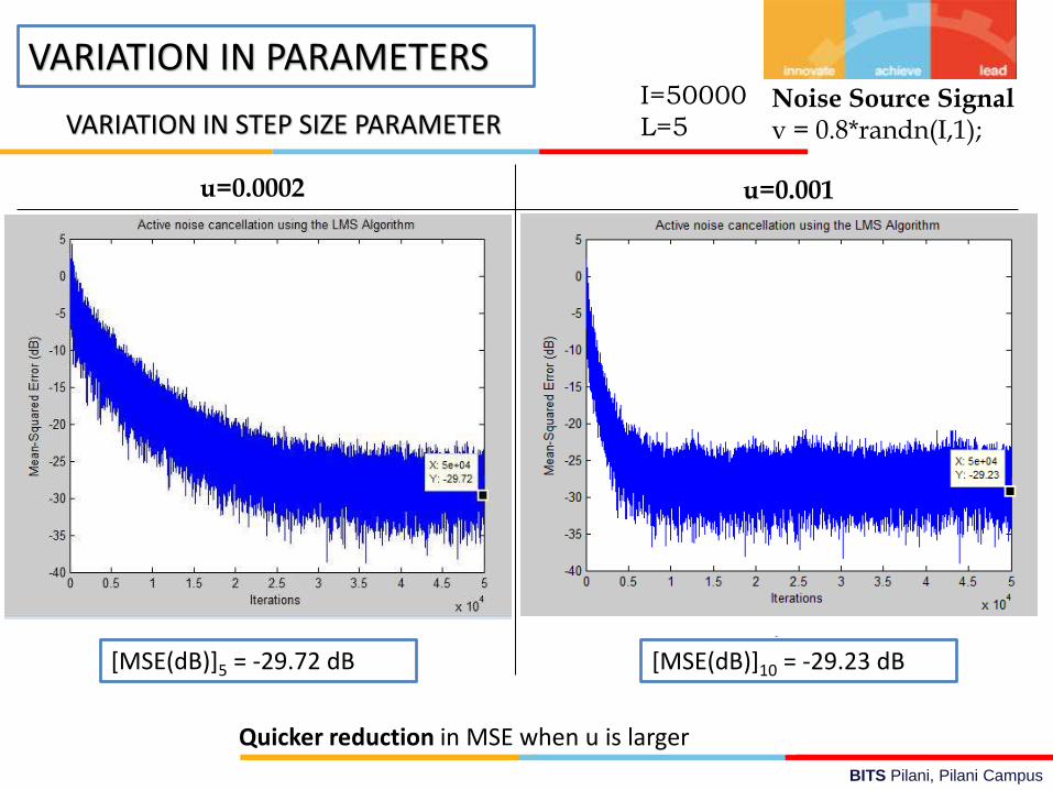
VARIATION IN PARAMETERS

VARIATION IN STEP SIZE PARAMETER

u=0.0002

Noise Source Signalv = 0.8*randn(I,1);

Quicker reduction in MSE when u is larger

[MSE(dB)]5 = -29.72 dB [MSE(dB)]10 = -29.23 dB

I=50000

L=5

u=0.001

BITS Pilani, Pilani Campus

ANC has been done for Single Tone Signal here.

Real Test begins, when the signal is a speech signal.

For that we will use the LMS Block in the Data

Acquisition Toolbox of Matlab.