abstract representation of object and structural symmetries detection

Abstract Representation of Object and Structural

Symmetries Detection

Vincent Dugat(IRIT-UPS, Toulouse, France

[email protected])

Pierre Gambarotto(IRIT-UPS, Toulouse, France

[email protected])

Yannick Larvor(IRIT-UPS, Toulouse, France

[email protected])

Abstract: This paper describes a method for constructing an abstract representationof a shape from a classical polyhedral 3D representation of an object. This framework issuitable for qualitative reasoning. As an application we use this abstract representationto compute the structural symmetries of a 3D polyhedron. The starting point of thecomputation is a classical polyhedral 3D representation of the object. From the MedialAxis Transform (MAT) of this object we propose a more abstract representation basedon a set of spheres extracted from the MAT and structured as one or several graphs.This framework can be used for several purposes. Here we focus on the problem offinding structural symmetries of the object. We use the automorphisms group of thecomputed graphs. Then we propose a method to compute the automorphisms thathave a geometrical sense among the set of all automorphisms. We compare the bruteforce algorithm with a branch and bound strategy based on the orbits partition of thevertices.

Key Words: Qualitative reasoning, spatial reasoning, shape recognition, spatial rep-resentation, medial axis transform.Category: I.2.4, I.3.5.

1 Introduction

Two majors fields in AI are concerned with representation of objects: roboticson the one hand, and qualitative spatial reasoning (henceforth QSR) on theother. Robotics’ analysis tools are traditionally issued from classical physicaland mathematical science. Such tools are especially accurate to process rawnumerical data coming from robot’s sensors. On the contrary, QSR focuses onmore abstract representations, and puts the emphasis on qualitative relationsand expressive power rather than numerical precision. This manichean view isnot satisfying, for many reasons: robots sensors will (at least for some time) con-tinue to provide numerical data, but needs in intelligent behavior require higher

Journal of Universal Computer Science, vol. 9, no. 9 (2003), 1008-1029submitted: 10/2/03, accepted: 9/6/03, appeared: 28/9/03 © J.UCS

levels of abstraction, for instance in order to interact with human language, orfor sophisticated pathfinding algorithms.

There still remains a gap between the result of the treatment of numericaldata (by various techniques such as mesh reconstruction, boundary extraction,etc.) and qualitative reasoning on abstract entities.

In this article, we propose a method to construct an abstract representationmerging numerical and abstract informations. We start from objects representedin two or three dimensions: each object is built from a set of vertices, and eachvertex is located with coordinates in a Cartesian space. The final objective is toexpress the structure of such an object in an abstract framework. As an appli-cation we expose a method to express the structural symmetries of a 3D convexpolyhedron using the constructed framework. Note that this abstract frameworkallows different levels of granularities in this kind of computation. The startingpoint is a classical 3D representation of the object. We shall first expose theabstract representation of the shape: from the Medial Axis Transform (MAT) ofthis object is extracted a set of spheres structured in a graph which can be usedfor several purposes such as shape identification or shapes comparison. In thispaper we shall focus on the problem of finding the symmetries in the structure ofthe shape. We shall used the graph representation and tools of algebraic graphtheory such as a branch and bound algorithm based on automorphism groupresults. Sections 2 exposes the construction of the Medial Axis Transform andsection 3 focuses on the construction of the structure graph and other associatedgraphs extracted from the MAT in order to construct our abstract represen-tation. As an application, section 5 exposes a graph-theory based method forgenerating automorphisms that have a geometric sense opposing the brute forcealgorithm to an ad-hoc branch and bound one. Last, we precise that in the restof this paper the terms form and shape will be synonymous.

2 Constructing the MAT

The first step of our representation is to construct the medial axis transform.We shall detail this construction in the subsections that follow.

2.1 MAT: definition

The computation of the MAT is a complex task. We first define some notationsbefore detailing the construction algorithm:

• IR represents the set of real numbers; R3 denotes the standard Euclidean

space.

• The word ”distance” denotes hereafter the Euclidean distance in R3.

1009Dugat V., Gambarotto P., Larvor Y.: Abstract Representation of Object ...

• Let c be a point of R3 and r ∈ IR. The set of points whose distance from c

is less than or equal to r is called the (closed) ball of center c and radius r.

• In this paper, only the 3-dimensional case is considered. The 2D case can betreated with only minimal changes in the vocabulary used (mainly replace”ball” with ”disc”).

The Medial Axis (MA) of an object is defined as the locus of the centers ofits maximal interior balls. A ball inside an object is maximal iff it is containedin the object and is not a subset of another ball inside the object1. The radiusfunction denotes the function that associates to a point of the MA the radius ofthe corresponding maximal ball. The Medial Axis Transform of an object is theMA of this object together with the associated radius function.

With the notations introduced above, this definition becomes:

Definition 1 Let S be a subset of R3. The Medial Axis of S, noted M(S), is

the set of the centers of all maximal ball inside S, together with the limit pointsof this set.

Definition 2 The value at each M(S)’s point of the radius function r is theradius of the associated maximal ball. The values of this function are in IR, andr is continuous on M(S).

Definition 3 The Medial Axis Transform of the subset S of R3 is constituted

by M(S) and r.

2.2 Computation of MAT

In this paper, and for the sake of simplicity, we only consider the case of poly-hedra with simply connected face2. This restriction can be bypassed by subdi-viding multiply connected faces into simply connected faces. Such a decomposi-tion is described in the appendix B of [Sherbrooke et al., 1996]. The algorithmused to compute the MAT of a polyhedra is a slightly simplified version of[Sherbrooke et al., 1996]. This algorithm has the advantages of being exact andof having a polynomial complexity (in terms of number of faces).

2.2.1 Classification of MAT’s points

Each particular point of the MA is linked to several faces, as explained in thefollowing definition:1 Although we consider Euclidean 3-dimensional space, the only prerequisite of this

definition is a metric space2 Intuitively, a face is simply connected if it has no hole.

1010 Dugat V., Gambarotto P., Larvor Y.: Abstract Representation of Object ...

JP JPES

MS

EP

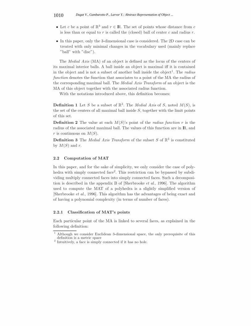
JP : junction point MS : middle seamES : end seamEP : seam end point

Figure 1: MA Points

Definition 4 Let p be a point on the MA of the polyhedral P. Let Br(p) bethe corresponding maximal sphere centered on p, of radius r. Let q1,. . . ,qn bethe points on the boundary of the object where Br(p) is tangent. The qi arecalled footpoints of p. If ji designates the index of the face, edge or vertex onwhich qi lies, then Pji is said to be a governor of p.

When considering only non degenerated cases, a particular point of the MAis obtained for each set of governors. With the notations introduced above, thespecific points of the MAT used in our algorithm3 are:

Junction Point : defined by four non degenerated governors.

Seam Point : defined by three non degenerated governors. For given governors,the set of seam points is generally a curve called a seam.

Seam-End Point : intersection of the boundary of the object and a seam ofthe MAT.

Sheet Point : defined by two non degenerated governors. Connected sheetpoints form a surface, called a sheet.

End Point : intersection of the boundary of the object and a sheet. A connectedset of end points is called a rim.

End seam : a seam between a junction point and a seam-end point (i.e. a vertexof the polyhedron).

In figure 1 are represented particular points of the MA of a parallelepiped.3 For more information on the MAT algorithm and further details in the classification

of points of the MAT, refer to ([Sherbrooke, 1995]).


61

5

34

2

1,5,6

1,3,6

3,5,61,3,5

1,3,5,6

Figure 2: MAT of a rectangular box

2.2.2 Principle of Sherbrooke’s algorithm

The above classification is primordial for the algorithm computing the medialaxis as it is shown in [Brand, 1992], the behavior of the MA near a MA pointis completely determined by the configuration of the point’s footpoints, or inother terms by the set of governors of this point. For instance, a junction pointalways lies at the junction of seams and a seam is at the intersection of sheets.This relation is made more evident by considering the governors set of each ofthese different elements. For instance, a seam is obtained with a set of threegovernors in the general case. Two intersected seam will have two governors incommon, and the junction point will thus have four governors. More generally,the governors’ set of an intersection is obtained by the union of the governors’set of the intersected parts of the MA.

The idea of the algorithm developed in [Sherbrooke et al., 1996] is to use thereverse property: when you have found a junction point, you calculate its set ofgovernors (by looking at its footpoints). Each subset of the junction point’s set ofgovernors is then checked to determine if it governs one of the seams intersectingat the junction point.

For the check, an initial tangent (i.e. at the junction point) is found byderivation of the system of governors’ equations. The building of the seam isthen achieved by integration of this system.

This algorithm is particularly simple when considering a convex polyhedra.In this case, all the parts of the MA connecting particular points are straight lines(and not general curves), and the corresponding system of equation is trivial.The integration can even be symbolically resolved.

At the vicinity of a concavity, the result of this MAT algorithm is generallymuch more complicated to obtain, because the MA may be locally a non degen-erated curve or a non degenerated surface (i.e. not a line or a plane). The calculusof those elements can be obtained by an approximated method of integration(for instance by a Runge Kutta method).

Example: on figure 2 is represented a rectangular box and the associated MA(without the limit points constituted by the rims and the seam end points). Thehighlighted junction point’s set of governors is 1, 3, 5, 6. To find the possibleseams intersecting at this point, we check every subset of three elements: 1, 3, 5,


⎧⎪⎪⎪⎪⎪⎨⎪⎪⎪⎪⎪⎩

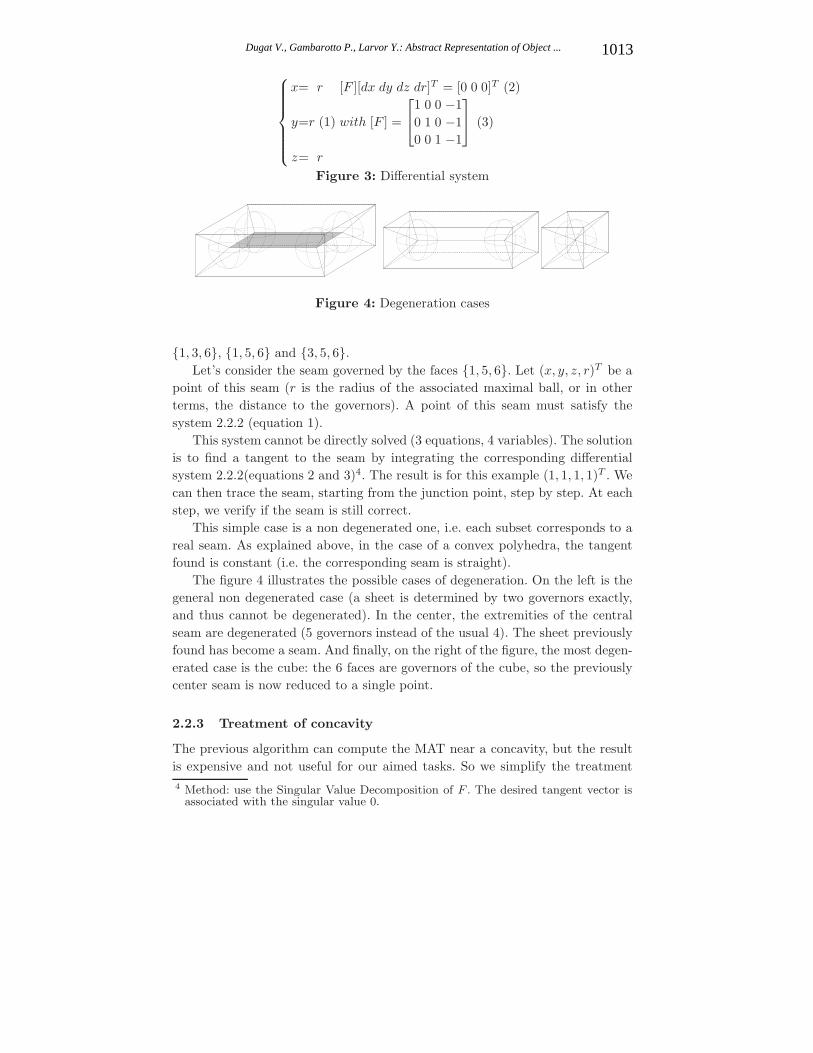
x= r [F ][dx dy dz dr]T = [0 0 0]T (2)

y=r (1) with [F ] =

⎡⎣

1 0 0 −10 1 0 −10 0 1 −1

⎤⎦ (3)

z= r

Figure 3: Differential system

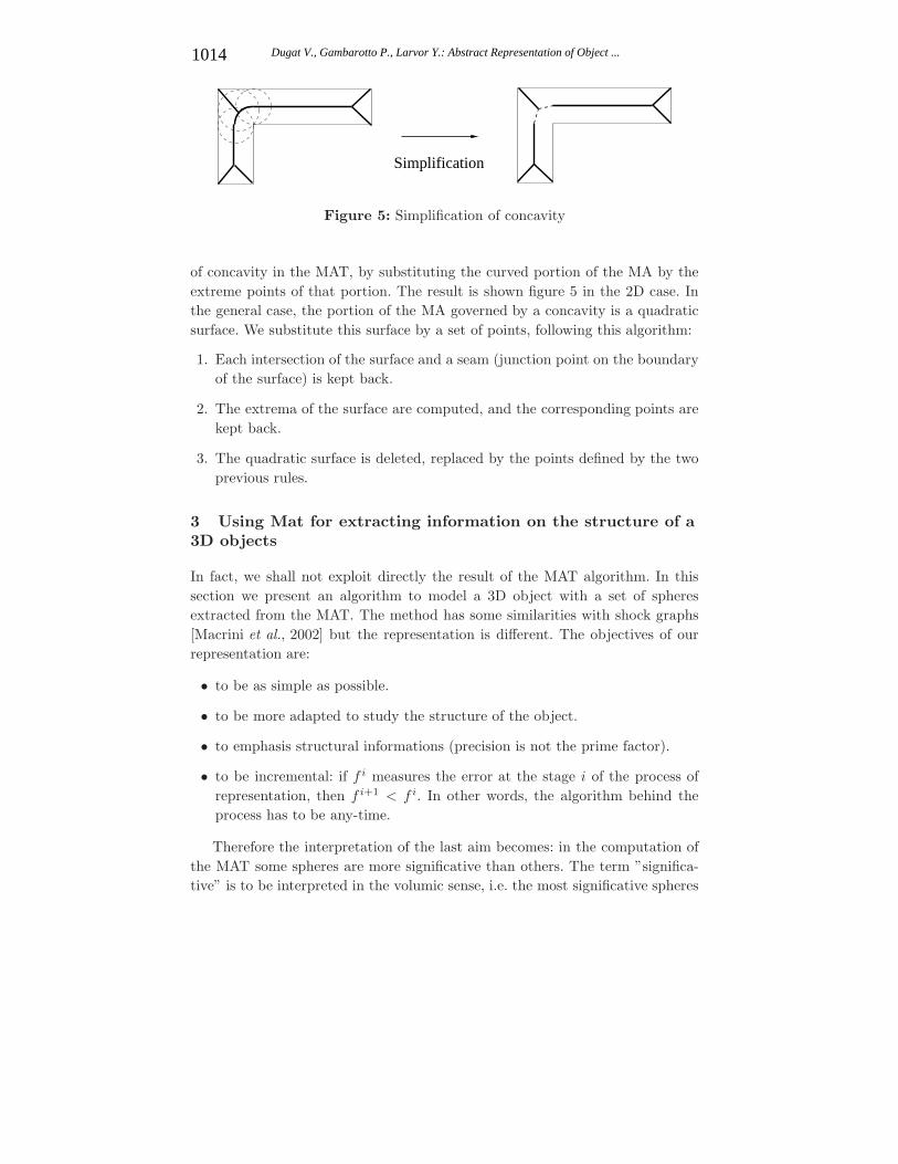
Figure 4: Degeneration cases

1, 3, 6, 1, 5, 6 and 3, 5, 6.Let’s consider the seam governed by the faces 1, 5, 6. Let (x, y, z, r)T be a

point of this seam (r is the radius of the associated maximal ball, or in otherterms, the distance to the governors). A point of this seam must satisfy thesystem 2.2.2 (equation 1).

This system cannot be directly solved (3 equations, 4 variables). The solutionis to find a tangent to the seam by integrating the corresponding differentialsystem 2.2.2(equations 2 and 3)4. The result is for this example (1, 1, 1, 1)T . Wecan then trace the seam, starting from the junction point, step by step. At eachstep, we verify if the seam is still correct.

This simple case is a non degenerated one, i.e. each subset corresponds to areal seam. As explained above, in the case of a convex polyhedra, the tangentfound is constant (i.e. the corresponding seam is straight).

The figure 4 illustrates the possible cases of degeneration. On the left is thegeneral non degenerated case (a sheet is determined by two governors exactly,and thus cannot be degenerated). In the center, the extremities of the centralseam are degenerated (5 governors instead of the usual 4). The sheet previouslyfound has become a seam. And finally, on the right of the figure, the most degen-erated case is the cube: the 6 faces are governors of the cube, so the previouslycenter seam is now reduced to a single point.

2.2.3 Treatment of concavity

The previous algorithm can compute the MAT near a concavity, but the resultis expensive and not useful for our aimed tasks. So we simplify the treatment4 Method: use the Singular Value Decomposition of F . The desired tangent vector is

associated with the singular value 0.


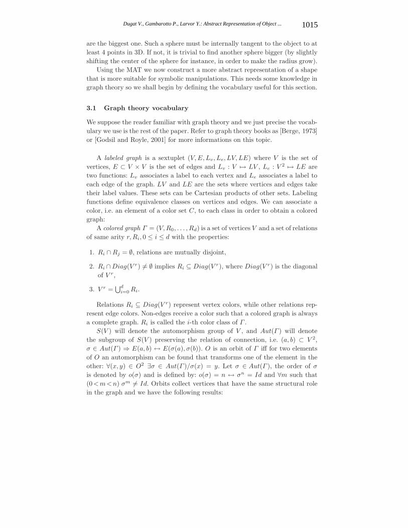
Simplification

Figure 5: Simplification of concavity

of concavity in the MAT, by substituting the curved portion of the MA by theextreme points of that portion. The result is shown figure 5 in the 2D case. Inthe general case, the portion of the MA governed by a concavity is a quadraticsurface. We substitute this surface by a set of points, following this algorithm:

1. Each intersection of the surface and a seam (junction point on the boundaryof the surface) is kept back.

2. The extrema of the surface are computed, and the corresponding points arekept back.

3. The quadratic surface is deleted, replaced by the points defined by the twoprevious rules.

3 Using Mat for extracting information on the structure of a3D objects

In fact, we shall not exploit directly the result of the MAT algorithm. In thissection we present an algorithm to model a 3D object with a set of spheresextracted from the MAT. The method has some similarities with shock graphs[Macrini et al., 2002] but the representation is different. The objectives of ourrepresentation are:

• to be as simple as possible.

• to be more adapted to study the structure of the object.

• to emphasis structural informations (precision is not the prime factor).

• to be incremental: if f i measures the error at the stage i of the process ofrepresentation, then f i+1 < f i. In other words, the algorithm behind theprocess has to be any-time.

Therefore the interpretation of the last aim becomes: in the computation ofthe MAT some spheres are more significative than others. The term ”significa-tive” is to be interpreted in the volumic sense, i.e. the most significative spheres


are the biggest one. Such a sphere must be internally tangent to the object to atleast 4 points in 3D. If not, it is trivial to find another sphere bigger (by slightlyshifting the center of the sphere for instance, in order to make the radius grow).

Using the MAT we now construct a more abstract representation of a shapethat is more suitable for symbolic manipulations. This needs some knowledge ingraph theory so we shall begin by defining the vocabulary useful for this section.

3.1 Graph theory vocabulary

We suppose the reader familiar with graph theory and we just precise the vocab-ulary we use is the rest of the paper. Refer to graph theory books as [Berge, 1973]or [Godsil and Royle, 2001] for more informations on this topic.

A labeled graph is a sextuplet (V, E, Lv, Le, LV, LE) where V is the set ofvertices, E ⊂ V × V is the set of edges and Lv : V → LV , Le : V 2 → LE aretwo functions: Lv associates a label to each vertex and Le associates a label toeach edge of the graph. LV and LE are the sets where vertices and edges taketheir label values. These sets can be Cartesian products of other sets. Labelingfunctions define equivalence classes on vertices and edges. We can associate acolor, i.e. an element of a color set C, to each class in order to obtain a coloredgraph:

A colored graph Γ = (V, R0, . . . , Rd) is a set of vertices V and a set of relationsof same arity r, Ri, 0 ≤ i ≤ d with the properties:

1. Ri ∩ Rj = ∅, relations are mutually disjoint,

2. Ri ∩Diag(V r) = ∅ implies Ri ⊆ Diag(V r), where Diag(V r) is the diagonalof V r,

3. V r =⋃d

i=0 Ri.

Relations Ri ⊆ Diag(V r) represent vertex colors, while other relations rep-resent edge colors. Non-edges receive a color such that a colored graph is alwaysa complete graph. Ri is called the i-th color class of Γ .

S(V ) will denote the automorphism group of V , and Aut(Γ ) will denotethe subgroup of S(V ) preserving the relation of connection, i.e. (a, b) ⊂ V 2,σ ∈ Aut(Γ ) ⇒ E(a, b) ↔ E(σ(a), σ(b)). O is an orbit of Γ iff for two elementsof O an automorphism can be found that transforms one of the element in theother: ∀(x, y) ∈ O2 ∃σ ∈ Aut(Γ )/σ(x) = y. Let σ ∈ Aut(Γ ), the order of σ

is denoted by o(σ) and is defined by: o(σ) = n ↔ σn = Id and ∀m such that(0<m<n) σm = Id. Orbits collect vertices that have the same structural rolein the graph and we have the following results:


Proposition 1 An orbit is invariant by an automorphism of Aut(Γ ): O is anorbit of Γ ⇒ ∀σ ∈Aut(Ω) σ(O) = O.

Proposition 2 An automorphism σ can be entirely described by its cycles. Theorder of σ is the lcm (least common multiple) of the lengths of the cycles of σ.

An automorphism of order 2 is said to be an involution. Let σ ∈ S(V ).The ordered set c = a0 a1 · · · an−1 an is a σ cycle of length n iff c ⊂ V ,∀i ∈ [1 · · ·n] σ(ai) = ai−1, ai−1 = ai and an = a0. Least, let σ ∈S(G). O ⊂ V

is said to be fixed with respect to σ iff: ∀x ∈ O σ(x) = x. This notion can beextended to a set of vertices called a block.

Computing the automorphism group of a graph is a hard task. Even ifthe problem is not known to be NP-complete there is at this date no poly-nomial algorithm. Fortunately there are efficient programs based on arbores-cent technics such as [McKay, 2000] or the Weisfeiler-Leman (WL) Algorithm[Babel et al., 1997].

A planar graph is a graph that can be drawn without crossing edges. Hopcroftand Wong established in [Hopcroft and Wong, 1974] that computing the auto-morphisms group is polynomial for planar graphs.

3.2 Sphere representation: construction of the structure graph

Sherbrooke’s algorithm for computing MAT works on any polyhedron as ex-plained in section 2.2.3. As said at the end of the same section we introduce asimplification of the MAT near a concavity. This reduces the number of spheresneeded to represent a concavity and allows an easier detection of maximal convexparts. In fact, we can observe that there is one or two spheres for each concavityof the object. We call theses spheres: articulation spheres.

The result of our representation is derived from a subset of the MAT, i.e. aset of Br(p) spheres (Cf. def 4). The spheres are selected in three consecutivestages. The second stage deals with end-seams and it could loop until the desiredgranularity is reached. In fact, in such a process, all the spheres of the end-seamwill be tangent to the previous and next computed ones. Moreover, their centerswill be on the same line and the ratio of two consecutive spheres is the same.So we do not need to loop in the second stage and compute only the two firstspheres on the end-seam: the first one to compute the ratio of their sizes (Cf.figure 6).

The core set of spheres is given by the spheres centered on junction point.For a more accurate precision, more spheres are added on seams pointing to avertex of the polyhedron:


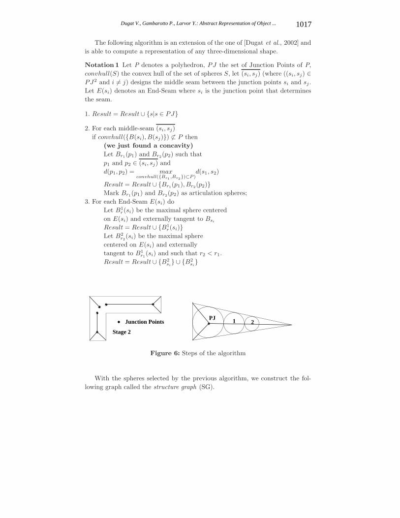
The following algorithm is an extension of the one of [Dugat et al., 2002] andis able to compute a representation of any three-dimensional shape.

Notation 1 Let P denotes a polyhedron, PJ the set of Junction Points of P,convhull(S) the convex hull of the set of spheres S, let (si, sj) (where ((si, sj) ∈PJ2 and i = j) designs the middle seam between the junction points si and sj .Let E(si) denotes an End-Seam where si is the junction point that determinesthe seam.

1. Result = Result ∪ s|s ∈ PJ

2. For each middle-seam (si, sj)if convhull(B(si), B(sj)) ⊂ P then

(we just found a concavity)Let Br1(p1) and Br2(p2) such thatp1 and p2 ∈ (si, sj) andd(p1, p2) = max

convhull(Bs1 ,Bs2)⊂P )d(s1, s2)

Result = Result ∪ Br1(p1), Br2(p2)Mark Br1(p1) and Br2(p2) as articulation spheres;

3. For each End-Seam E(si) doLet B1

r (si) be the maximal sphere centeredon E(si) and externally tangent to Bsi

Result = Result ∪ B1r(si)

Let B2r2

(si) be the maximal spherecentered on E(si) and externallytangent to B1

r1(si) and such that r2 < r1.

Result = Result ∪ B2si ∪ B2

si

1

Junction Points 2

Stage 2

PJ

Figure 6: Steps of the algorithm

With the spheres selected by the previous algorithm, we construct the fol-lowing graph called the structure graph (SG).


Definition 5 The structure graph SG = (V, E) is a labeled graph such that:

V is the set of vertices called spheres. All the spheres are those computed bythe Sphere Representation algorithm and belonging to the MAT,

E is the set of edges i.e. a binary relation defined by: (x, y) ∈ E if x and y arerelated by a seam the MAT.

We have two functions defining labels on vertices and edges:

• Ls, which associates to each sphere the labels defining a type from (PJ ,END, ART ) and one or two sizing coefficients:

• (PJ, size) if the sphere is centered on a junction point, and the size is theratio between the sphere and a reference one (the biggest in the MAT).

• (END, size, ρ) if the sphere has its center on a end-seam, size is the ratiobetween the sphere and the reference one, and ρ the ratio of decreasingsize on the end-seam.

• (ART, size) if the sphere has been marked as an articulation sphere.

• Le : E −→ IR+, which associates to each edge a distance (ratio) betweenthe two spheres that define the edge. Note that in case of an edge between asphere centered at a junction point and a sphere centered on an end-seam,the distance is null since they are tangent.

As a geometric graph, SG is a subset of the MAT since we consider all spheresat junction points, and the shape is uniquely represented by such a graph.

Moreover, we associate to this graph a function D : V → IR3, mapping avertex with the coordinates of the center of the associated sphere that will beuseful is some applications.

The resulting representation is simple as requested. We can observe thatthere is a sphere for each concavity of the object. This representation seems tobe adequate to study the structure of an object.

Note that if the object is convex the previous algorithm reduces to points 1and 3.

Example: The figure 7 shows a 2D convex form with the discs computedby 3.2 and the associated graph with labels. The labels of the vertices are theratios wrt the biggest sphere.

3.3 Convex part graph and convex parts structure graph of theform

The structure graph of a concave shape can be complex. In order to have amore flexible representation, this graph can be splited in several parts. From


2

3

4

5(2/(sqrt(2)−1))(2/(sqrt(2)−1))

(2/(sqrt(2)−1))(2/(sqrt(2)−1))

(1)

(0)

(0)(0)

(0)

1

Figure 7: A convex form and its associated labeled structure graph

the structure graph is extracted a set of subgraphs called Convex Part Graphs(CPG) and corresponding to maximal convex parts. The convex hull of the setof spheres belonging to such a subgraph gives a rather accurate approximationof the shape of the part. Each sphere graph corresponding to a maximal convexpart is delimited in the CPG by two sets of articulation spheres detected at stage2 of the algorithm in section 3.2.

We now need to know the relations between the CPG, so we construct a newgraph we call Convex parts structural graph CPSG = (A, R), where:

• A = p1, . . . , pk, where k is the number of maximal convex parts and eachpi is associated with a maximal convex part of SG,

• ∀(pi, pj) ∈ A × A, (pi, pj) ∈ R iff the associated convex parts Pi and Pj aresuch that: if Ai and Aj are the sets of articulation spheres of Pi and Pj , thenAi and Aj are connected by some edge in SG.

4 Construction of a colored graph

From the structure graph SG = (V, E) (or CPG and CPSG) we construct acolored graph Γ , that is to say that we define colors on vertices and on edges:(i). Two vertices x and y will have the same color iff the spheres correspondingto x and y have the same size and, (ii) two edges will have the same color iff thedistance between their corresponding extremity spheres is the same. Non-edgescorrespond to a color in order to complete the graph.

The equivalence classes of colors define a partition of the set V of vertices.This partition can be refined to obtains the partition into orbits of the automor-phisms group of the graph using a so-called branch and bound method. This isthe topic of the next section.


The construction of such a colored graph is necessary to compute automor-phisms group with methods as Weissfeiler-Leman or Nauty, that are useful insome applications of the abstract framework described here ([Dugat et al., 2002]).

5 Structural Analysis of a 3D form

One application of the structure graph is the detection of properties of the shape.Properties we will focus on here are structural invariance by isometries. Wewill call theses transformations symmetries. Symmetry detection in graph andgeometric interpretation is a classic problem in graph drawing and is known tobe NP-hard [Eades and Lin, 2000], [Hong, 2002]. Our problem is quite different:to detect symmetries that have a geometric sense in the form. The method weare about to expose will be used on structure graph. That is to say on the entirestructure graph. But we can also modulate the granularity, i.e. in the case of aconvex shape we can consider only the spheres of the first step of the algorithmin section 3.2 (those on the PJ points), to detect symmetries on the main partof the shape avoiding “details”. On concave shapes the computation can focuson CPG or CPSG to detect symmetries on the parts independently one of theother, or on the main relational structure of theses parts.

5.1 General results on symmetries

In order to understand what kind of problem we deal with here, we need someresults on symmetries and graph structure.

Definition 6 [Abelson et al., 2002] A symmetry α of a set of points Q in IR3 isan isometry IR3 → IR3 such that α(Q) = Q.

As explained in [Hong, 2002], symmetries in the three dimensional space canby classified as rotation, reflection, inversion and rotary reflection:

• Rotational symmetry is a rotation about an axis ;

• Reflectional symmetry is a reflection in a plane ;

• Inversion is a reflection in a point ;

• Rotary reflection is a composition of a rotation and a reflection.

We only focus in this paper on rotations and reflections, i.e. the three firsttypes of symmetries. If the shape is invariant by reflection or rotation then thecenter of the isometry can be materialized by vertices in the spheres graph ornot.


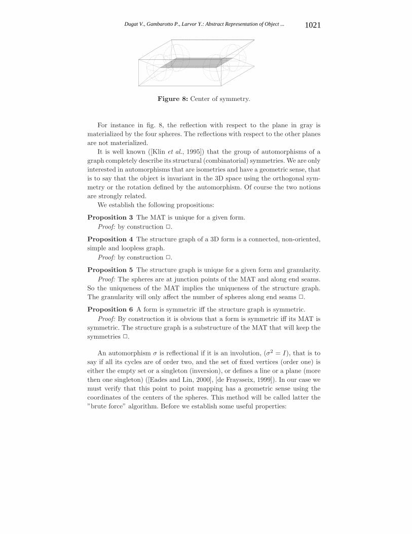
Figure 8: Center of symmetry.

For instance in fig. 8, the reflection with respect to the plane in gray ismaterialized by the four spheres. The reflections with respect to the other planesare not materialized.

It is well known ([Klin et al., 1995]) that the group of automorphisms of agraph completely describe its structural (combinatorial) symmetries. We are onlyinterested in automorphisms that are isometries and have a geometric sense, thatis to say that the object is invariant in the 3D space using the orthogonal sym-metry or the rotation defined by the automorphism. Of course the two notionsare strongly related.

We establish the following propositions:

Proposition 3 The MAT is unique for a given form.Proof: by construction .

Proposition 4 The structure graph of a 3D form is a connected, non-oriented,simple and loopless graph.

Proof: by construction .

Proposition 5 The structure graph is unique for a given form and granularity.Proof: The spheres are at junction points of the MAT and along end seams.

So the uniqueness of the MAT implies the uniqueness of the structure graph.The granularity will only affect the number of spheres along end seams .

Proposition 6 A form is symmetric iff the structure graph is symmetric.Proof: By construction it is obvious that a form is symmetric iff its MAT is

symmetric. The structure graph is a substructure of the MAT that will keep thesymmetries .

An automorphism σ is reflectional if it is an involution, (σ2 = I), that is tosay if all its cycles are of order two, and the set of fixed vertices (order one) iseither the empty set or a singleton (inversion), or defines a line or a plane (morethen one singleton) ([Eades and Lin, 2000], [de Fraysseix, 1999]). In our case wemust verify that this point to point mapping has a geometric sense using thecoordinates of the centers of the spheres. This method will be called latter the”brute force” algorithm. Before we establish some useful properties:


An automorphism σ is a rotation ([Eades and Lin, 2000] if each cycle hasorder k, possibly except for several cycles with size one defining a line. A cycleC of σ with order k can be represented by x, σ(x), σ2(x), . . . , σk−1(x) for anyx of C.

Proposition 7 Let σ ∈ Aut(SG). The cycles of σ form partitions which are arefinement of the orbits partition of the vertices of SG.

Proof: Let (x0, x1, . . . , xk) be a cycle of σ. We have ∀i ∈ 0, k−1, xi+1modk =σ(xi). So all the elements of the cycle belong to the same orbit of Aut(SG).Cycles are disjoint hence they define a refinement of the orbit partition of theset of vertices .

Proposition 8 Let σ ∈ Aut(SG) be a geometric symmetry. If there are spheresof SG belonging to the center of symmetry of σ then these spheres are fixed byσ.

Proof: Fixed elements are invariant by σ. So if it is a geometric symmetry,invariant elements must be on the center of symmetry .

Proposition 9 Let σ be a geometric symmetry of Aut(SG) then all pairs(x, σ(x)) of σ are of order two and their middle belongs to the center of symmetryof σ.

Proof: Obvious .

5.2 The convex part case

Convex shapes are particular cases that have interesting computational proper-ties:

Proposition 10 The structure graph of a 3D convex form is planar.Proof: In the MAT, spheres are a measure of the thickness of the form, all

in the same direction because of the convexity of the form and the maximalityof the spheres. Moreover, when sheets and seams meet in the MAT we place asphere, so the structure graph can be drawn without edges crossing and then isplanar .

Hong gives in [Hong, 2002] the following result:

Proposition 11 There is a polynomial time algorithm which computes a max-imum size three dimensional symmetry group for planar graphs.

So in this special case combinatorial symmetries are computed in polynomialtime for the structure graph SG = (V, E). Each such symmetry is an automor-phism σ mapping V on itself. For each couple (v, σ(v)) we must then verifythe compatibility D(v) and D(σ(v)) wrt the isometry corresponding to σ in theEuclidean space.


5.3 General 3D form case

In order to compute the orbits partition of the graph vertices, we use a branchand bound method as the Weisfeler-Leman algorithm ([Babel et al., 1997]) orBrandan McKey’s software Nauty based on a similar approach ([McKay, 2000]).Note that Nauty can also compute the complete group of automorphisms.

The above methods expect colored graphs, and to use them we interpret ourlabeled sphere graph as a colored graph as shown in section 4.

From the orbits partition of the set of vertices of the structure graph, we wantto compute the automorphisms that are geometric isometries. We have severalstrategies: generate all the automorphisms with softwares are Nauty and selectthose that we want, or try to compute directly the interesting automorphisms.The next section compares the two strategies.

5.3.1 Brute force algorithm for general graphs

We shall show in this section that the brute-force algorithm can not be an efficientsolution of computation. First we expose its principle:

1. Compute all the automorphisms of SG,

2. Keep in the previous set the automorphisms of order two (reflection) or k > 2(rotation),

3. Keep in the previous set the automorphisms whose set of fixed points isempty or is composed of:

• one vertex, rectilinear vertices or coplanar vertices in the case of theorder two,

• rectilinear vertices in the case of order k > 2,

4. In the case of a reflection, compute the middle of each cycle of σ, and verifywith the coordinate function D that the middles are all rectilinear or coplanarand are compatible by an orthogonal symmetry whose center is the fixedpoints set if it is not empty.

5. In the case of a rotation compute the axis of the rotation of each cycle of σ

and verify with D that the points are all rectilinear and are compatible witha rotation whose axis is the fixed points set if it is not empty.

Note: if the shape is convex the points 1 to 3 are replaced by: compute themaximal symmetry group

For sake of simplicity we only expose here the case of reflectional symmetry.Given a graph SG, the desired algorithm has to check for each automorphism σ


of Aut(SG) whether σ corresponds to a geometric reflection of the object whoseSG is the structure graph.

Let σ be an automorphism of Aut(SG). σ represents a geometric reflection ifand only if it verifies the three following properties (with SG = (V , C, Lv, Le,LV , LE) as defined in section 3.1):

1. σ ∈ Aut(SG), i.e.:

• ∀a ∈ V Lv(σ(a)) = Lv(a)

• ∀(a, b) ∈ V 2 Le(σ(a), σ(b)) = Le(a, b)

• ∀(a, b) ∈ V 2 E(a, b) ↔ E(σ(a), σ(b))

2. The order of σ is 2, i.e. σ is a reflection (thus not the identity function)

3. σ is a geometric reflection, i.e. ∀(a, b) ∈ V 2 such that a = b (σ = Id so it isalways possible to find (a, b) ∈ V 2 such that a = b), σ(a) = b, A = D(a) andB = D(b) are the associated geometric points of the vertices a and b, P isthe plane perpendicular to the line (AB) that intersects (AB) in M , middleof [A, B], σ verifies one of the following properties:5

Planar symmetry with regard to P :

• ∀(c, d) ∈ V 2 if c = d and σ(c) = d, then P is perpendicular to theline (CD) and intersects [CD] in its middle .

• ∀e ∈ V/ σ(e) = e, then E ∈ P .

Central symmetry with regard to M :

• ∀(c, d) ∈ V 2 if c = d and σ(c) = d, then M middle of [CD].

• ∀e ∈ V if σ(e) = e, then E = M .

Axial symmetry :

• ∃(c, d) ∈ V 2−(a, b), (b, a)/ c = d and σ(c) = d, N middle of [CD],then N ∈ P .

• ∀(e, f) ∈ V 2/ e = f , σ(e) = f , and O middle of [EF ], then O ∈(MN).

• ∀g ∈ V/ if σ(g) = g then G ∈ (MN).

5 For the sake of simplicity, if the lowercase letter ”a” designs a vertex of SG, thenthe uppercase letter ”A = D(a)” stands for the associated geometric point.


The main problem of this method is its computational complexity in thegeneral case. For instance if the shape is a cube we have a sphere graph composedof one sphere centered on the unique junction point and eight spheres tangentwith the previous one and located on end seams (if we stop algorithm of section3.2 at step 2.j for j = 1). This graph with nine vertices has 40320 automorphisms.Only 13 are geometric symmetries: six are symmetries with respect to planesdefined by opposite edges of the cube and three defined by the middles of paralleledges, three are symmetries with respect to lines defined by the center of oppositefaces, one is a central symmetry. So it is more suitable to compute directlythe automorphisms we are interested in, which can be done for the cube withtheoretical algebraic graph tools since it is a convex shape, but not in the generalconcave case. So in the next section we present a branch and bound method tocompute directly symmetric automorphisms.

5.3.2 Branch and bound algorithm for geometric symmetries re-search

We saw that the complexity of the naive algorithm (the above called ”bruteforce”) is exponential. To reduce the complexity, two different strategies can beenvisaged:

1. Divide the research space.

2. For a given search space, try not to explore the whole associated searchgraph.

The first strategy is rather easy to apply: instead of doing the search forsymmetries on the whole set of vertices of a graph SG, this can be done on eachsubset corresponding to the orbits. This property is directly derived from thedefinition of an orbit: considering an automorphism that would associate twovertices from two different orbits is useless, because the corresponding automor-phism will not be a member of Aut(SG), and thus not be a symmetry.

The second strategy is more complex: we gradually constrain the possiblecentral element of symmetry. Given a central element and an orbit, we considerthe permutation of two elements in this orbit. We check whether this permutationis compatible with the central element. The different possibilities are detailed inthe graph in appendix A. The function realizing this evolution is the functionevo: given a possible central element and an elementary permutation x|y (x andy are possibly the same element), it returns the new possible central element,if any. This function is called recursively by SymOrbit which is applied on eachorbit while there is still a possible central element. If a candidate element remainsafter examining all orbits, then a geometrical symmetry has been found.

Let o1, o2, . . . , on be the partition of Γ into orbits. The method is imple-mented by the following algorithm:


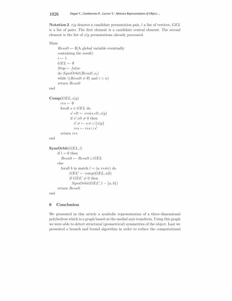
Notation 2 x|y denotes a candidate permutation pair, l a list of vertices, GEL

is a list of pairs. The first element is a candidate central element. The secondelement is the list of x|y permutations already processed.

MainResult ← ∅(A global variable eventuallycontaining the result)i ← 1GEL ← ∅Stop ← false

do SymOrbit(Result, oi)while ((Result = ∅) and i < n)return Result

end

Comp(GEL, x|y)res ← ∅forall s ∈ GEL do

s′.elt ← evo(s.elt, x|y)if s′.elt = 0 then

s′.σ ← s.σ ∪ x|yres ← res ∪ s′

return res

end

SymOrbit(GEL, l)if l = 0 then

Result ← Result ∪ GEL

elseforall b in match l = (a, reste) do

GEL′ ← comp(GEL, a|b)if GEL′ = 0 thenSymOrbit(GEL′, l − a, b)

return Result

end

6 Conclusion

We presented in this article a symbolic representation of a three-dimensionalpolyhedron which is a graph based on the medial axis transform. Using this graphwe were able to detect structural (geometrical) symmetries of the object. Last wepresented a branch and bound algorithm in order to reduce the computational


complexity of the method in the general case. This is a first step for reasoning onabstract representations of objects and is an alternative to pure computationalgeometry or pure logical representations.

References

[Abelson et al., 2002] David Abelson, Seok-Hee Hong, and Donald Taylor. A group-theoretic method for drawing graphs symmetrically. Technical Report TechnicalReport IT-IVG-2002-01, School of Information Technologies, University of Sydney,2002.

[Babel et al., 1997] L. Babel, I.V. Chuvaeva, M. Klin, and D.V. Pasechnik. Algebraiccombinatorics in mathematical chemistry. methods and algorithms. ii. program im-plementation of the weisfeiler-leman algorithm, 1997.

[Berge, 1973] Claude Berge. Graphs and hypergraphs. North-Holland, 1973.[Brand, 1992] J. Brand. Describing a solid with three-dimentional skeleton. In J. D.

Warren, editor, Proceeding of the International Society for Optical Engineering, vol-ume 1830, pages 258–269, 1992.

[de Fraysseix, 1999] Hubert de Fraysseix. An heuristic for graph symmetry detection.In Graph Drawing, volume 1731 of Lecture Notes in Computer Science, Springer,pages 276–285, 1999.

[Dugat et al., 2002] Vincent Dugat, Pierre Gambarotto, and Yannick Larvor. Qual-itative Geometry for Shape Recognition. In Applied Intelligence, volume 17, pages253–263. Kluwer Academic Publishers, novembre 2002.

[Eades and Lin, 2000] Peter Eades and Xuemin Lin. Spring algorithms and symmetry.Theoretical Computer Science, 240(2):379–405, 2000.

[Godsil and Royle, 2001] Cris Godsil and Gordon Royle. Algebraic Graph Theory.Springer, 2001.

[Hong, 2002] Seok-Hee Hong. Drawing graphs symmetrically in three dimensions. InGraph Drawing, 9th International Symposium, Vienna, Austria, September 2001,LNCS 2265, pages 189–204. Springer, 2002.

[Hopcroft and Wong, 1974] J. Hopcroft and J. Wong. Linear time algorithm for iso-morphism of planar graphs. Sixth Annual ACM Symp. on Theory of Computing,pages 172–184, 1974.

[Klin et al., 1995] M. Klin, C. Rucker, G. Rucker, and G. Tinhofer. Algebraic combi-natorics in mathematical chemistry, 1995.

[Macrini et al., 2002] Diego Macrini, Ali Shokoufandeh, Sven Dickinson, Kaleem Sid-diqi, and Steven Zucker. View-based 3-d object recognition using shock graphs.In 16 th International Conference on Pattern Recognition (ICPR’02), Quebec City,Canada, volume 3, 2002.

[McKay, 2000] Brendan McKay. Nauty user’s manual. Australian National University,Cambera, 2000.

[Sherbrooke et al., 1996] Evan Sherbrooke, Nicholas Patrikalakis, and Erik Brisson.An algorithm for the medial axis transform of 3d polyhedral solids. IEEE Trans. onVisualisation and Comp. Graphics, 2(1):44–61, 1996.

[Sherbrooke, 1995] Evan Sherbrooke. 3D Shape Interrogation by Medial Axis Trans-form. PhD thesis, MIT, Cambridge, Massachusets, 1995.

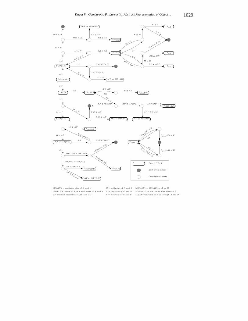
A Annex: Evolution function

We present the principle of the Branch and Bound algorithm as a graphic whichresumes the different steps. How to read the graph on next page:


• Vertices in thick rounded box are entry and/or exit points, depending onwhether the arcs lead from and/or to them. They bear as labels the geomet-rical element given to/returned by the function emphevo. The arcs leavingthese nodes are only labeled with the pair we try to add to the current au-tomorphism.The vertices labeled S/elt correspond to the case when we have found adefinite reflectional element elt, be it a plane, line or point.

• Round grey vertices mark a dead end: the tested configuration is impossible,evo returns a void central element.

• Round blank vertices mark testing points. Arcs stemming from them bearmutually exclusive conditions, which are tests on the possible geometric con-figurations at these points in the graph.


S/elt

a|b

p|pS /elt

(P) =

P

S/elt(P ) = P

S/elt (A) =

B

S/elt(A) = B

∆= common mediatrix of AB and CD

LM(L, XY )=true iff L is a medriatrix of X and Y

MP(XY ) = mediator plan of X and Y LMP(AB) = MP(AB) or ∆ or M

LP(P )= P or any line or plan through P

LL(AP )=any line or plan through A and P

a|b

c|d

M = N

AB ‖ CD

AB ∦ CD

EF ∈ ABC

M = R

LM(∆, EF )

E ∈ ∆

c|c C ∈ MP(AB)

p|p

a|b

a|ab|b

B ∈ AP

P M ⊥ AB

P M ⊥ AB

AP ∈ MP(BC) AP ∈ MP(BC)

LP(P ) S/(ABP )

S/(MN)

S/∆

S/∆

d|e

MP(DE) = MP(BC)

AB ∦ CD

C = M

M or ∆

LL(AP )

d|d

D ∈ APS/(DAP )

B ∈ AP

MN = ∆

AB‖ CD

D ∈ MP(BC)

M=

P

b|c

C=

M

E ∈∆

¬LM(∆, E

F)

e|f

e|e

M = P

D ∈ AP

C ∈ MP(AB)

MC or MP(AB)

MA or MP(BC)

S/MP(DE)

LMP(AB)

AP ∩ BC = ∅

AP ∩ BC = ∅S/MP(BC)

AP or MP(BC)

AP or MP(BC)

LMP(AB)

AP or MP(DE)

S/M

S/(AP)

Entry / Exit

Exit with failure

Conditional state

D ∈ MP(BC)

¬LM(AP, D

E)

MN or MP(CD)

AP ∩

DE = ∅

AP ∩ DE = ∅

MP(DE) = MP(BC)

LM(A

P, DE)

M = midpoint of A and B

N = midpoint of C and D

R = midpoint of E and F

MN = ∆

M = N

E = M

EF ∈

AB

C

E=

M

Anything


abstract representation of object and structural symmetries detection

Documents