abella: a system for reasoning about relational speci cationsdale/papers/abella-tutorial.pdf ·...
TRANSCRIPT

Abella: A System for Reasoning about RelationalSpecifications
DAVID BAELDE KAUSTUV CHAUDHURI
LSV, ENS Cachan, France Inria & LIX/Ecole polytechnique, France
ANDREW GACEK DALE MILLER
Rockwell Collins, USA Inria & LIX/Ecole polytechnique, France
GOPALAN NADATHUR ALWEN TIUUniversity of Minnesota, USA Nanyang Technological University, Singapore
YUTING WANGUniversity of Minnesota, USA
The Abella interactive theorem prover is based on an intuitionistic logic that allows for inductiveand co-inductive reasoning over relations. Abella supports the λ-tree approach to treating syntax
containing binders: it allows simply typed λ-terms to be used to represent such syntax and it
provides higher-order (pattern) unification, the ∇ quantifier, and nominal constants for reasoningabout these representations. As such, it is a suitable vehicle for formalizing the meta-theory of
formal systems such as logics and programming languages. This tutorial exposes Abella incre-mentally, starting with its capabilities at a first-order logic level and gradually presenting more
sophisticated features, ending with the support it offers to the two-level logic approach to meta-
theoretic reasoning. Along the way, we show how Abella can be used prove theorems involvingnatural numbers, lists, and automata, as well as involving typed and untyped λ-calculi and the
π-calculus.
Contents
1 Introduction 31.1 A bit of history . . . . . . . . . . . . . . . . . . . . . . . . . . . . . . 31.2 Abstractions of syntax . . . . . . . . . . . . . . . . . . . . . . . . . . 31.3 The organization of this tutorial . . . . . . . . . . . . . . . . . . . . 4
2 The top-level structure of Abella 52.1 Types, terms, and formulas . . . . . . . . . . . . . . . . . . . . . . . 52.2 Some top-level commands . . . . . . . . . . . . . . . . . . . . . . . . 72.3 Interactive tactical theorem proving . . . . . . . . . . . . . . . . . . 8
3 Equality 11
Acknowledgements: We thank Andrea Asperti, Roberto Blanco, Zakaria Chihani and ClaudioSacerdoti Coen for their comments on drafts of this tutorial. This work has been partiallysupported by the NSF Grants OISE-1045885 (REUSSI-2) and CCF-0917140, by the INRIA
Associated Teams Slimmer and rapt, and by the ERC Advanced Grant ProofCert. Opinions,findings, and conclusions or recommendations expressed in this paper are those of the authors and
do not necessarily reflect the views of the National Science Foundation, the European ResearchCouncil, INRIA, ENS Cachan, Nanyang Technological University, or Rockwell Collins.
Journal of Formalized Reasoning Vol. ?, No. ?, Month Year, Pages 1–89.
2 · Baelde, Chaudhuri, Gacek, Miller, Nadathur, Tiu, & Wang
3.1 Basic examples . . . . . . . . . . . . . . . . . . . . . . . . . . . . . . 123.2 Proving that equality is a congruence . . . . . . . . . . . . . . . . . . 133.3 Peano axioms and the open-world assumption . . . . . . . . . . . . . 14
4 Relational specifications 144.1 Defining relations as fixed points . . . . . . . . . . . . . . . . . . . . 154.2 Some recursive definitions involving lists . . . . . . . . . . . . . . . . 174.3 Finite success and finite failure . . . . . . . . . . . . . . . . . . . . . 18
5 Induction and co-induction 205.1 Inductive hypotheses vs. inductive invariants . . . . . . . . . . . . . 235.2 Kinds of induction . . . . . . . . . . . . . . . . . . . . . . . . . . . . 24
5.2.1 Simple induction . . . . . . . . . . . . . . . . . . . . . . . . . 245.2.2 Mutual induction . . . . . . . . . . . . . . . . . . . . . . . . . 255.2.3 Nested and lexicographic induction . . . . . . . . . . . . . . . 26
5.3 Co-induction . . . . . . . . . . . . . . . . . . . . . . . . . . . . . . . 27
6 Reasoning about objects with bound variables 306.1 Representing constructs with bound variables . . . . . . . . . . . . . 316.2 The ∇ quantifier and nominal constants . . . . . . . . . . . . . . . . 326.3 Induction in the presence of the ∇ quantifier . . . . . . . . . . . . . 366.4 An enhancement to definitions . . . . . . . . . . . . . . . . . . . . . 38
7 Extended examples 417.1 The untyped λ-calculus . . . . . . . . . . . . . . . . . . . . . . . . . 417.2 Meta-theory of minimal intuitionistic logic . . . . . . . . . . . . . . . 437.3 The π-calculus . . . . . . . . . . . . . . . . . . . . . . . . . . . . . . 47
8 The Two-Level Logic Approach 568.1 Horn clause specifications . . . . . . . . . . . . . . . . . . . . . . . . 588.2 Hereditary Harrop specifications . . . . . . . . . . . . . . . . . . . . 618.3 Dynamic context management . . . . . . . . . . . . . . . . . . . . . 668.4 Exploiting the meta-theory of the specification logic . . . . . . . . . 718.5 General context relations . . . . . . . . . . . . . . . . . . . . . . . . 748.6 Extended example: Transitivity of subtyping in system Fsub . . . . . 76
9 Future Directions 82
A Summary of Abella syntax and commands 87
Journal of Formalized Reasoning Vol. ?, No. ?, Month Year.

Abella: A System for Reasoning about Relational Specifications · 3
1. INTRODUCTION
Abella is an interactive proof assistant designed to reason about relational inductiveand co-inductive specifications, with a particular emphasis on reasoning aboutrelations between terms containing bindings. Abella is available for download fromhttp://abella-prover.org.
1.1 A bit of history
The first version of the Abella theorem prover was developed by Andrew Gacek aspart of his doctoral work carried out at the University of Minnesota [19]. KaustuvChaudhuri and Yuting Wang have subsequently designed and implemented extensionsto the system, resulting in an updated release. The various authors of this tutorialand several of their colleagues have been involved in developing the theoreticalunderpinnings of this system, providing input on its structure and fleshing outexamples of its applications.
The Abella prover was originally designed to illustrate the possibility of reasoningdirectly over the relational judgments that can be constructed in λProlog [39] andin LF [29]. Even back in the 1990’s, it was clear that such relational specificationscould be extremely useful in a wide range of formalization efforts in the areasof proof systems [3, 15, 49], type systems [2, 14], and programming languagesemantics [26, 27, 28]. Of course, relational specifications have often been used in anumber of other domains such as relational databases and model checking as well.
Reasoning directly with judgments about higher-order objects, examples of whichwe shall first encounter in Section 6, presents a number of challenges to conventionaltheorem provers. One of those challenges is providing an abstract and flexibletreatment of bindings within syntax. The logic G is the result of a decade longeffort [5, 22, 34, 35, 43, 63, 64, 69] to design an increasingly more flexible andpowerful logic that would provide such a treatment of binding. The Abella proverhas allowed this work on proof theory to be validated and exploited within aninteractive theorem proving setting.
1.2 Abstractions of syntax
Computation and reasoning on linguistic structures goes back at least to Godel andChurch. For them, syntax was encoded as a string of symbols: we usually refer to thatapproach to syntax as concrete syntax. While concrete syntax has the advantage ofbeing readable and writable by humans, it has many disadvantages. Concrete syntaxcontains too much information that is not important for many manipulations, suchas white space, infix/prefix notation, and keywords; and important computationalinformation is not represented explicitly, such as recursive structure, function–argument relationship, and the term–subterm relationship. The field of parsing wasdeveloped in part to translate concrete syntax into more meaningful tree structures,often called parse trees. In such tree structures, much semantically meaninglessinformation is discarded and the recursive structure is made central.
For those attempting to reason about meta-theoretic properties of programs, typecheckers, compilers, theorem provers, etc., it has become clear that parse trees are notabstract enough. In particular, the way that parse trees encode binding structures(e.g., quantifiers, formal parameters, and lexical scopes) is too concrete. Treatingbinding using named variables (despite the fact that α-conversion makes the choice
Journal of Formalized Reasoning Vol. ?, No. ?, Month Year.

4 · Baelde, Chaudhuri, Gacek, Miller, Nadathur, Tiu, & Wang
of actual names that are used unimportant) or as De Bruijn-style offset counters iscomplex and adds many details to programs and specifications that are, in the end,orthogonal to real semantic content. As evidence of that problem, the POPLMarkchallenge [4] attempted to raise interest in the theorem proving community to makebetter tools for dealing with bindings in syntax so that formalized meta-theory couldbe made manageable.
There have been various attempts to treat bindings in syntax in a more abstractfashion. For example, one of the applications of nominal logic [53] has been toprovide a new approach to representing binders [18]. In this tutorial we will focus onusing λ-tree syntax [41], a third approach to syntactic representation. This approach,which is closely related to the higher-order abstract syntax approach [48], is directlysupported in λProlog. As we shall see in Section 6, one of the characteristics ofAbella is that it make it possible to reason on encodings of syntax at this level ofabstraction.
1.3 The organization of this tutorial
Abella is based on the logic G [21, 22] that contains several features that may appearnovel to the uninitiated reader. This tutorial is organized to introduce these featuresin an incremental fashion.
—At a propositional level, G makes use of the usual intuitionistic logical constants:true, false, conjunction, disjunction, and implication. In addition G possesses thetyped quantifiers ∀τ and ∃τ for all simple types τ that do not contain the type offormulas; these quantifiers are drawn from Church’s Simple Theory of Types [12].In Section 2, we present the basic structure of Abella that is built around theseconnectives and quantifiers.
—Equality at all simple types τ is treated as a logical connective in G. While theproof theory underlying this treatment is natural, it is not well-known in thetheorem proving community. We describe reasoning based on this connective inSection 3.
—Relational specifications are introduced into G via fixed point definitions. Section 4considers the treatment of such definitions in Abella.
—Inductive and co-inductive definitions of relations are supported in G by givingdefinitions a least or greatest fixed point reading. The treatment of induction andco-induction in Abella is presented in Section 5.
—Support for λ-tree syntax in G is dependent significantly on the ∇ (nabla) quan-tifier [6, 21, 42, 43] and the closely associated notion of nominal constants [22].Section 6 introduces these notions and demonstrates how they can be used totreat binding in syntax.
Once the logical features underlying Abella have been presented, we turn toshowing how they can be used in practical reasoning tasks. In Section 7 we illustratehow some of the meta-theory of logics and formalisms such as the π-calculus and the(untyped) λ-calculus can be captured in Abella. In Section 8, we finally consider howAbella can be used to reason about relational specifications written in λProlog. Wedescribe here the two level logic approach that allows such reasoning to be carriedout through an encoding of the derivability relation of the logic underlying λPrologin an Abella definition.
Journal of Formalized Reasoning Vol. ?, No. ?, Month Year.

Abella: A System for Reasoning about Relational Specifications · 5
At the outset of this tutorial, we shall assume that the reader is familiar with thenatural deduction or sequent calculus style of proof presentation of intuitionisticlogic. We shall also assume familiarity with the treatment of the standard logicalconnectives and quantifiers in such a proof-theoretic setting. Prior exposure toconcepts such as λ-tree syntax and the ∇ quantifier can be useful but is not assumed.A reader familiar with the Coq system [9] will also find many points of similarity inthe development of proofs in Abella, although we caution that there are significantdifferences as well.
Before commencing on the tutorial, we comment on the use of the term higher-order ; see also [39, Section I.3] for a related discussion. This term may or maynot apply to the logic G, depending on what exactly is meant by it. A type τ isconsidered to be higher-order if it has an arrow type to the left of another arrowtype. A minimum requirement for a logic to be higher-order is that it permitquantification over higher-order types. The logic G allows such quantification andmay therefore be considered higher-order. However, many people would require afurther property for the use of this adjective: quantification must be permitted overtypes that contain the type of formulas. Such quantification is not permitted in Gand hence it does not pass this test. Given the ambiguity in the term higher-orderwhen applied to G, we eschew its use in this tutorial.
2. THE TOP-LEVEL STRUCTURE OF ABELLA
This section gives an overview of the concrete syntax and command-level interactionwith Abella. Keeping to the spirit of a tutorial, we are not concerned here withpresenting all details necessary for successfully using Abella: for that, the interestedreader can find a user manual at http://abella-prover.org
2.1 Types, terms, and formulas
The concrete syntax of Abella is presented in this document using a monospacedfont: in addition, keywords are depicted in blue. The types, terms, and formulasused by Abella are described briefly below as well as in the table in Figure 1.
Types in Abella are the simple types; such types are either primitive types orbuilt from two types using the arrow type constructor →. The type constructor→ associates to the right, so every type in Abella can be written in the formτ1 → · · · → τn → b (for n ≥ 0) where b is an atomic type that is called its targettype, and each τi itself has this structure. User-defined atomic types are introducedby means of Kind declarations that we shall describe presently.
Terms in Abella are simply typed λ-terms built from variables, constants, λ-abstractions, and applications. Constants are introduced into Abella using the Type
declarations explained below. A λ-abstraction is written using an infix backslash (\).The scope of a λ-abstraction extends as far to the right as possible while remainingin the syntactic class of terms; thus, x\ f x stands for λx. (f x). Note that the leftoperand of \ must be a bound variable, possibly with a type ascription, so, eventhough \ has lower precedence than application, x\ f y\ y x is unambiguouslyparsed as λx. (f (λy. (y x))). Types for λ-bound variables may be omitted if theycan be inferred; type-inference must be be able to fill in all such missing types forthe term to be deemed well-formed.
Journal of Formalized Reasoning Vol. ?, No. ?, Month Year.

6 · Baelde, Chaudhuri, Gacek, Miller, Nadathur, Tiu, & Wang
Abstract Concrete Precedence/
Associativity
Types (τ)
Atomic types prop, nat, list, . . .Arrow types τ1 → τ2 T1 -> T2 right
Terms (m,n)Variables x, y, . . . x, y, . . .
Constants c, d, . . . c, d, . . .Nominal constants n1, n2, . . . n1, n2, . . .
(n followed by at least one digit)
Abstractions λx.m x\ M 0, rightλx:τ.m x:T\ M 0, right
Applications m n M N 5, left
Formulas (A,B)
Logical constants >,⊥ true, false
m = n M = N 4, noneAtomic formulas p m1 · · · mn p M1 ... Mn 5, left
Connectives A ∧B A /\ B 3, leftA ∨B A \/ B 2, left
A ⊃ B A -> B 1, right
Quantifiers ∀x.∀y:τ. . . . A forall x (y:T) ..., A 0∃x.∃y:τ. . . . A exists x (y:T) ..., A 0
∇x.∇y:τ. . . . A nabla x (y:T) ..., A 0
(parentheses required for type-annotations)The Abella user manual [71] gives details on the lexical structure of identifiers. Parentheses maybe used to explicitly indicate groupings, which is otherwise inferred using the precedence and
associativity rules in the fourth column.
Fig. 1: Concrete Syntax for G in Abella.
Formulas in Abella are written using the standard syntax as shown in Figure 1.Formulas are actually terms of type prop. Atomic formulas are formulas whosetop-level constructor is not a logical symbol (i.e., a logical constant, connective, orquantifier). In other words, the top-level constructor of an atomic formula must be auser defined constant with the target type prop. Such a constant is called a predicateor relational symbol. Predicate symbols can be introduced through Type declarationsor through the Define or CoDefine commands explained in Sections 4.1 and 5. Thescoping rules for the quantifiers of G are similar to those for λ-abstractions, and thetypes of such quantified variables may also be omitted when they can be inferreduniquely. Note that Abella does not allow quantification over variables whose typescontain the type prop. In particular, quantification is not permitted over predicatevariables, i.e., variables that have prop as their target type.
In the next several sections, we will not make explicit use of λ-abstractions interms: as a result, these sections will view Abella as being based on a fairly standardfirst-order logic. Starting in Section 6, the treatment of λ-bindings will play animportant role in our examples. It is also from that section on that we will allowformulas to contain the ∇ quantifier and terms and formulas to contain nominalconstants.
Journal of Formalized Reasoning Vol. ?, No. ?, Month Year.

Abella: A System for Reasoning about Relational Specifications · 7
2.2 Some top-level commands
Interacting with Abella involves issuing a sequence of commands: such commandsdeclare kinds and types, introduce definitions, state theorems and develop theirproofs. All such commands end with a full-stop. We can also intersperse commandswith comments. Comments take the form of line-comments that begin with thecharacter % that causes the rest of the line to be ignored, or with arbitrary textdelimited by a balanced pair of /* and */ (supporting nesting).
Declarations come in two varieties: declarations of new atomic types, and declara-tions of new constants. To declare a new atomic type, one uses a Kind declarationthat has the general form:
Kind b1 , ..., bn type.
where the b1, . . . , bn are pairwise distinct valid identifiers that are not alreadyatomic types declared earlier. Each of b1, . . . , bn is then added to the collection ofatomic types that may be used to form other types. The final keyword type is usedto indicate that these atomic types have kind type; this is somewhat redundantfor the simple type system of Abella, but allows for future extensions to the typesystem with higher kinded atomic types.
To declare a collection of constants c1, . . . , cn of a particular type T, one uses aType declaration that has the general form:
Type c1 , ..., cn T.
The type T must be formed out of atomic types that have been declared earlier bymeans of Kind declarations. Further, the constants c1, . . . , cn must be pairwisedistinct valid identifiers that are not already declared using Type or defined usingthe Define or CoDefine commands that we discuss later. Every Abella developmentbegins with a standard collection of type and constant declarations preloaded, shownin Figure 9 in the appendix.
As an example, here is how we would define a new atomic type nat of naturalnumbers, constants z and s to construct such numbers, and a type list of naturalnumbers with constants empty and cons to construct them.
Kind nat type.
Type z nat.
Type s nat -> nat.
Kind list type.
Type empty list.
Type cons nat -> list -> list.
It is important to note that the collection of constants of any type may be extendedat any time with new declarations. Thus, there is no guarantee that all terms oftype nat, for instance, are constructed using just z and s.
Another command in Abella is the one that proposes a formula to be consideredfor proof. This command has the following general form:
Theorem thm_name : A.
where thm_name is any valid identifier that is distinct from other constants declaredor defined earlier, and A is a formula. Abella uses the same keyword Theorem for all
Journal of Formalized Reasoning Vol. ?, No. ?, Month Year.

8 · Baelde, Chaudhuri, Gacek, Miller, Nadathur, Tiu, & Wang
flavors of provable formulas – lemmas, propositions, corollaries, etc. Every theoremmust be followed by its proof, which is a series of tactics: we start introducingtactics in Section 2.3. Interactions with Abella are often called developments. Suchdevelopments can be entered either interactively or via batch files: in the lattercase, the files are given names with the suffix .thm. Such files can be piped directlyto the abella program or can be given as the first command line argument to theprogram. Abella processes the file and outputs its interaction history to standardoutput until it encounters an error (which causes an immediate abort of the programexcept in the interactive top-level) or it finishes processing all the commands in thefile. In the interactive top-level, Abella uses the prompt
Abella <
to indicate that it is ready for top-level commands, and prompts of the form
thm_name <
to indicate that it is expecting tactics to prove the theorem named thm_name.
2.3 Interactive tactical theorem proving
So far, we have seen a few top-level commands of Abella—namely, Kind, Type, andTheorem. In order to prove a theorem in Abella, we use tactic commands insteadof top-level commands, which are depicted in brown text. The set of tactics inAbella is small and fairly close to the inference rules of G. These tactics will beintroduced gradually in this document, and each theorem name will be linked toa website where the effects of the tactics can be browsed without needing to runAbella separately. Nevertheless, the reader is encouraged to follow along by copyingthe proofs that are presented in this document directly into the Abella top-level, orusing one of the provided source files for the accompanying on-line materials withthis tutorial.
When proving a theorem, Abella maintains a stack of subgoals, with the topmostsubgoal of the stack selected as the current goal. Initially, there is only a singlesubgoal which is the theorem itself, but certain tactics may create additional subgoalsthat are pushed on to the subgoal stack. The current subgoal is presented in theinteraction history of Abella in the following general form:
Variables: x1 ... xm
H1 : A1
...
Hn : An
============================
C
where x1, . . . , xm are universally quantified variables, H1, . . . , Hn are hypothesislabels that are each associated with a unique hypothesis formula drawn from A1,. . . , An and C is a formula called the conclusion of the goal. The collection ofvariables and hypotheses is called the context of the goal. If there are no universallyquantified variables, the Variables line is omitted entirely. Note also that each ofthe variables that are shown has a type associated with it, even though this type isnot explicitly presented. At each intermediate stage in the development of a proof,
Journal of Formalized Reasoning Vol. ?, No. ?, Month Year.

Abella: A System for Reasoning about Relational Specifications · 9
only the current goal is shown in full; only the conclusion is shown for the remainingsubgoals.
Whenever a tactic is processed by Abella, it transforms the current goal as relevantand then displays the new proof state. As an illustration, suppose that we providethe following declarations
Kind i type.
Type p prop.
Type q i -> prop.
and then try to prove the following theorem.
Theorem extr : forall y, (p -> forall x, q x) -> p -> q y.
Abella displays the initial proof state as follows:
============================
forall y, (p -> (forall x, q x)) -> p -> q y
extr <
We can use the intros tactic to introduce all the antecedents, which yields:
extr < intros.
Variables: y
H1 : p -> (forall x, q x)
H2 : p
============================
q y
Now we can use the apply tactic that takes two hypotheses and uses implication-elimination (modus ponens) on them to get a new hypothesis.
extr < apply H1 to H2.
Variables: y
H1 : p -> (forall x, q x)
H2 : p
H3 : forall x, q x
============================
q y
Finally, we can use the backchain tactic to match the conclusion of a goal againstthe head of a hypothesis: if that match works, then the body of that hypothesisbecomes the conclusion of the new goal.
extr < backchain H3.
Proof completed.
Abella <
Abella re-enters the top-level command processing state when a proof is complete.For another example of proving a theorem, consider the following.
Journal of Formalized Reasoning Vol. ?, No. ?, Month Year.

10 · Baelde, Chaudhuri, Gacek, Miller, Nadathur, Tiu, & Wang
Kind nat type.
Type z nat.
Type s nat -> nat.
Type p nat -> prop.
Theorem four : (forall x, p x -> p (s x)) ->
p z -> p (s (s (s (s z)))).
intros.
At this point, there is one current goal:
H1 : forall x, p x -> p (s x)
H2 : p z
============================
p (s (s (s (s z))))
We could use backchain H1 four times to complete this proof. An alternative is touse the assert tactic to introduce a local lemma. The tactic invocation assert A
causes the current goal to be split into two subgoals: one where the conclusion ischanged to A and the other that is identical to the current goal except that A isadded to the hypotheses. For the above subgoal, this would look as follows:
four < assert (forall x, p x -> p (s (s x))).
Subgoal 1:
H1 : forall x, p x -> p (s x)
H2 : p z
============================
forall x, p x -> p (s (s x))
Subgoal is:
p (s (s (s (s z))))
four <
Observe that there are now two subgoals to prove. The first, which is displayed infull detail, can be proved by two applications of the backchain H1 tactic.
four < intros.
Subgoal 1:
Variables: x
H1 : forall x, p x -> p (s x)
H2 : p z
H3 : p x
============================
p (s (s x))
Subgoal is:
p (s (s (s (s z))))
four < backchain H1.
Journal of Formalized Reasoning Vol. ?, No. ?, Month Year.

Abella: A System for Reasoning about Relational Specifications · 11
Subgoal 1:
Variables: x
H1 : forall x, p x -> p (s x)
H2 : p z
H3 : p x
============================
p (s x)
Subgoal is:
p (s (s (s (s z))))
four < backchain H1.
H1 : forall x, p x -> p (s x)
H2 : p z
H3 : forall x, p x -> p (s (s x))
============================
p (s (s (s (s z))))
four <
Now, having successfully proved that formula, it is available as a hypothesis and wecan return to proving our original goal. This proof can be completed by two uses ofthe backchain tactic, but this time using the hypothesis H3.
We shall continue to introduce tactics one-by-one as we have occasion to use themin example proofs. The Abella tactics used in this tutorial are briefly describedin Figure 7 of the appendix; the full list, including precise documentation of theirsemantics, can be found in the Abella manual [71].
3. EQUALITY
The most basic relation in Abella, as it is in many theorem provers, is term equality.A distinguishing characteristic of G, the logic underlying Abella, is that equalityis treated as a logical connective with its own introduction rules and a role incut elimination [22, 25, 34, 60]. In order to understand the treatment of equality,one must understand the nature of terms: Abella employs the free term algebra,which means that terms are finitely constructed from term constructors that areinjective and distinct. Thus, the only way to prove an equality conclusion t = sis for t and s to be syntactically identical.1 Conversely, an equality hypothesist = s can be analyzed by considering all the ways in which t and s can be madeidentical. Unification is useful for this purpose. If t and s fail to unify, then theequality hypothesis is absurd and the goal is immediately proved. Otherwise, wecan transform the entire goal into a set of other goals where, first, the hypothesist = s is removed and, second, a unifier of t and s is applied to all the remaininghypotheses and conclusion formula. The unifiers that are considered in such atransformation must cover all possible unifiers of t and s. In this section, wherewe restrict our attention to only first-order terms, we use the most general unifiers
1The logic assumes the λ-conversion rules so in fact we mean identical with respect to these rules.
Journal of Formalized Reasoning Vol. ?, No. ?, Month Year.

12 · Baelde, Chaudhuri, Gacek, Miller, Nadathur, Tiu, & Wang
that are known to exist for this purpose. Later, when we work with arbitrarysimply typed λ-terms, we use the generalization of this notion to complete sets ofunifiers [31]. In practice, Abella restricts attention to unification problems to thehigher-order pattern fragment [37, 47] where, once again, most general unifiers areguaranteed to exist.
3.1 Basic examples
To illustrate the basic rules of equality, consider the following script where we declarea type i, equip it with a few term constructors, and set out to prove a few resultsabout terms at type i.
Kind i type.
Type a, b, c i.
Type g i -> i.
Type f i -> i -> i.
Theorem ex1 : exists x, x = a.
witness a. search.
In the proof of ex1, we choose a as a witness for the existentially quantified variablex. This yields a subgoal with a trivial equality as conclusion, and we discharge itusing the search tactic.
As another example, consider the following script.
Theorem ex2 : forall x y z,
f x (g y) = f (g y) z -> x = z.
intros. case H1. search.
In this example, after introducing the three eigenvariables and the equality hypothesisunder the name H1, we eliminate the hypothesis using case. As a result, Abellacomputes the most general unifier for the two terms in hypothesis H1, namely thesubstitution θ = [x 7→ (g y), z 7→ (g y)], and then applies that substitution to allformulas in the full goal. This then gives rise to the trivial conclusion formulag y = g y and the search tactic is able to complete the proof.
As we have observed above, unification may not always succeed. This is the casein the following example.
Theorem ex3 : a = b -> false.
intros. case H1.
Here, the application of the case tactic to H1 results in an attempt to unify a andb. This attempt fails and thereby the proof is trivially completed.
As a slightly more elaborate example of equality reasoning, consider proving thatthe set {a, c} is included in {a, b, c}. Although Abella does not have a built-innotion of sets2, we can represent them by their membership predicates, that isλx. (x = a ∨ x = c) and λx. (x = a ∨ x = b ∨ x = c). (We will discover a nicer wayto encode such sets in the next section.) Using this idea, we can express our setinclusion, and prove it as follows.
2 The curly brackets {, } will be used in Section 8 but not to denote sets.
Journal of Formalized Reasoning Vol. ?, No. ?, Month Year.
Abella: A System for Reasoning about Relational Specifications · 13
Theorem ex4 : forall x,
x = a \/ x = c -> x = a \/ x = b \/ x = c.
intros. case H1. search. search.
In this instance, the case tactic deals with the disjunction and its two equalitydisjuncts. This tactic generates two subgoals, in which x has been unified with aand b respectively, resulting in the conclusion formulas a = a ∨ a = b ∨ a = c andc = a ∨ c = b ∨ c = c. Each subgoal is immediately proved using search, since itsconclusion formula contains a trivial equality as a disjunct.
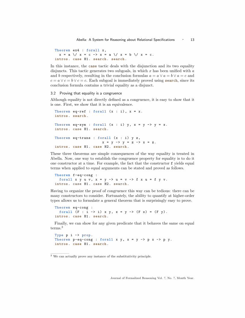
3.2 Proving that equality is a congruence
Although equality is not directly defined as a congruence, it is easy to show that itis one. First, we show that it is an equivalence.
Theorem eq-ref : forall (x : i), x = x.
intros. search.
Theorem eq-sym : forall (x : i) y, x = y -> y = x.
intros. case H1. search.
Theorem eq-trans : forall (x : i) y z,
x = y -> y = z -> x = z.
intros. case H1. case H2. search.
These three theorems are simple consequences of the way equality is treated inAbella. Now, one way to establish the congruence property for equality is to do itone constructor at a time. For example, the fact that the constructor f yields equalterms when applied to equal arguments can be stated and proved as follows.
Theorem f-eq-cong :
forall x y u v, x = y -> u = v -> f x u = f y v.
intros. case H1. case H2. search.
Having to organize the proof of congruence this way can be tedious: there can bemany constructors to consider. Fortunately, the ability to quantify at higher-ordertypes allows us to formulate a general theorem that is surprisingly easy to prove.
Theorem eq-cong :
forall (F : i -> i) x y, x = y -> (F x) = (F y).
intros. case H1. search.
Finally, we can show for any given predicate that it behaves the same on equalterms.3
Type p i -> prop.
Theorem p-eq-cong : forall x y, x = y -> p x -> p y.
intros. case H1. search.
3 We can actually prove any instance of the substitutivity principle.
Journal of Formalized Reasoning Vol. ?, No. ?, Month Year.

14 · Baelde, Chaudhuri, Gacek, Miller, Nadathur, Tiu, & Wang
3.3 Peano axioms and the open-world assumption
Given the nature of constructors and their treatment by equality, it is possible toprove two of Peano’s axioms for describing the natural numbers. In the followingdevelopment, the type of natural numbers is introduced as are the constructors forzero and successor. The injectivity of successor and the difference between zero andsuccessor are simple to state and prove.
Kind nat type.
Type z nat.
Type s nat -> nat.
Theorem succ-inj : forall x y, (s x) = (s y) -> x = y.
intros. case H1. search.
Theorem zero-succ : forall x, (s x) = z -> false.
intros. case H1.
In addition, we have a simple proof of the fact that no number is its own successor.
Theorem finiteness : forall x, x = (s x) -> false.
intros. case H1.
This theorem holds because x is quantified over finite terms, a fact reflected in theproof through the failure of unification. It is important to note that we did not andcould not use an induction on x here. In fact, Abella does not allow case analysisdirectly on terms—as a result, it is not possible to prove forall (x : nat), x =
z \/ exists y, x = s y. This goes with another key principle of Abella: we donot assume the signature to be closed, and so all reasoning should remain valid if thesignature is extended later. Of course, closedness assumptions are often necessary;they shall be expressed by means of user-defined relations, a topic we discuss in thenext section.
4. RELATIONAL SPECIFICATIONS
There are two basic approaches to defining operations such as addition on the termsbuilt from the constructors z and s declared in the previous section; these approachescan be seen as answers, respectively, to the questions of “how” and “what.” The firstis the functional approach—a response to the “how” question—where a computationsum explicitly builds the sum of a pair of nats by analyzing the structure of itsinputs. The inputs and outputs of the function are fixed; one cannot use the samefunction to compute the difference of two numbers. Moreover, the computationsinteract with the notion of equality on terms; for instance, it must be the case that:
sum (s z) (s (s z)) = s (s (s z))
It would be incorrect here to observe that the topmost “function” symbol of the twoterms being compared are different and therefore that the terms must be different.To compare terms with such embedded computations for equality, we must, therefore,extend the equational theory of terms to account for such computations.
The alternative is the relational approach—a response to the “what” question—where we define a relation plus between three nats that asserts that the third nat
is the sum of the first two. In other words, plus is not a way to construct new
Journal of Formalized Reasoning Vol. ?, No. ?, Month Year.

Abella: A System for Reasoning about Relational Specifications · 15
nats from old, but is an assertion about nats that are constructed with just z ands, with no change to their equational theory. Indeed, the plus predicate can bedefined in terms of a simple inference system with the following inference rules.
plus z N Nplus M N K
plus (s M) N (s K)
To establish that m and n sum to k, it suffices to find a derivation of plus m n kusing the inference system above. The plus inference system can, moreover, be usedjust as easily for subtraction: the same derivation establishes that n is the differenceof m and k. Finally, if k is not the sum of m and n, then there is no derivation ofplus m n k, so the inference system is a complete characterization of addition.
4.1 Defining relations as fixed points
Abella directly realizes the relational approach by means of relational fixed pointdefinitions often just called fixed points. To illustrate, the inference system for plusabove is represented in Abella using the following definition.
Define plus : nat -> nat -> nat -> prop by
plus z N N ;
plus (s M) N (s K) := plus M N K.
The target type of the plus predicate is the type prop of formulas of G; every suchdefinition must have the target type prop. Each inference rule above is capturedas a definitional clause for the plus predicate, with all the clauses separated bysemi-colons. The head of each clause is the atomic formula that occurs to the left of:=, while the formula to the right of := is the body. (If there is no := in a clause,the body is implicitly set to true.) In each clause, the capitalized identifiers—the M,N, K, etc.—are assumed to be universally quantified, so the clause stands for everyinstance of these identifiers.
This fixed point definition has the same properties as the plus inference system.It can establish true facts such as:
Theorem plus_two_two :
plus (s (s z)) (s (s z)) (s (s (s (s z)))).
unfold 2. unfold 2. unfold 1. search.
We could have proved this with just search, but we have used explicit unfoldsto show which definitional clause of plus was used to unfold the conclusion; seeFigure 7 for the semantics of unfold. More importantly, the plus definition canalso be used to show the negation of incorrect summations.
Theorem plus_bad : plus (s (s z)) (s z) (s (s z)) -> false.
intros. case H1. case H2. case H3.
Note that in the uses of unfold or case above, the goal or the hypothesis is of theform plus M N K which is matched against one of the heads of the definitional clausesof plus, and the corresponding body is used to replace the goal or the hypothesis.It is possible to view each definition as implicitly constructing a disjunction of allits definitional clauses, with the variables explicitly quantified. Thus, an explicitversion of the plus relation may be written as follows.
Journal of Formalized Reasoning Vol. ?, No. ?, Month Year.

16 · Baelde, Chaudhuri, Gacek, Miller, Nadathur, Tiu, & Wang
Define plus_ex : nat -> nat -> nat -> prop by
plus_ex M N K :=
(M = z /\ K = N)
\/ (exists M’ K’, M = s M’ /\ K = s K’ /\ plus M’ N K’).
The two relations plus and plus_ex are equivalent, but plus is easier to use becausethe disjunctions are left implicit both in its definition and in proofs involving plus.
These implicit disjunctions can also be used to enumerate the elements of afinite relation explicitly. For example, the sets {a, b} and {a, b, c}, defined usingdisjunction and equality in Section 3, can equivalently be defined as relations:
Define ab : i -> prop by
ab a ; ab b.
Define abc : i -> prop by
abc a ; abc b ; abc c.
Theorem ex4_defs : forall x, ab x -> abc x.
intros. case H1. search. search.
The ex4_defs theorem, which is the version of ex4 from Section 3 using definitions,has an identical proof. We will revisit such explicit enumerations when discussinginductive invariants in the next section.
To give a logical meaning to relational fixed point definitions, we have to ensurethat the fixed point being declared to exist actually does exist. To see the danger,consider a putative definition such as:
Define p : prop by
p := p -> false.
We can prove both p and p -> false by simply unfolding and case-analysis of p:4
Theorem p_true : p.
unfold. intros. case H1 (keep). apply H2 to H1.
Theorem notp_true : p -> false.
intros. case H1 (keep). apply H2 to H1.
Abella complains about such a definition by emitting a warning that the definitionfails the stratification condition, which is a sufficient condition to ensure that thefixed point exists [34, 63]. A definition for a predicate p is stratified if in itsdefinitional clauses there are no occurrences of p in subformulas to the left of animplication and only those predicates that have previously been defined are used.Note that this condition is per definition; any definition that follows the definitionof p can use p without restrictions, just as the definition of p can freely use anypredicate that has been defined earlier.
4 The default behavior for the case tactic is to remove the hypothesis that has just been analyzed
by it. Sometimes, however, it convenient or necessary to keep that hypothesis since it will be used
another time. In such cases, we use the expression (keep) with the tactic as we have done here.Interestingly, it has been shown in [25, 60] that producing contradictions such as the one underdiscussion using fixed points requires using a hypothesis more than once.
Journal of Formalized Reasoning Vol. ?, No. ?, Month Year.

Abella: A System for Reasoning about Relational Specifications · 17
The stratification condition used by Abella is conservative. For example, thefollowing two definitions fail this condition.
Define q : prop by
q := (q -> false) -> false.
Define r : nat -> prop by
r z ;
r (s N) := r N -> false.
Recent results [8, 69] suggest that definitions of the first kind may be permittedwithout loss of consistency. Similarly, a weakened version of stratification hasbeen identified that renders the second definition acceptable [66]. An alternativedevelopment permits definitions of the second kind in a form that does not allowcase analysis to be done on them, treating them instead as recursive definitions inthe style of Coq [8]. A further discussion of this matter is beyond the scope of thistutorial. Suffice it to say that any warnings of the violation of the stratificationcondition emitted by Abella must be given serious consideration for fear of permittingdefinitions that introduce inconsistencies.
4.2 Some recursive definitions involving lists
Consider the example of lists of natural numbers below:
Kind list type.
Type empty list.
Type cons nat -> list -> list.
Define memb : nat -> list -> prop by
memb N (cons N L) ;
memb N (cons M L) := memb N L.
We can then directly define the standard set inclusion and equality.
Define set_incl : list -> list -> prop by
set_incl S T :=
forall E, memb E S -> memb E T.
Define set_eq : list -> list -> prop by
set_eq S T := set_incl S T
/\ set_incl T S.
Once we have defined the memb relation in this way, we can use it in the formexists E, memb E S /\ pred E, where it is serves to check membership in a set(encoded as the list S), and in the form forall E, memb E S -> pred E, where itis used to define the range of such a set. Observe that if there are repetitions ofelements in the list representing a set, then the memb relation may enumerate thatelement more than once.
The sets ab and abc that we constructed above as definitions can instead be builtexplicitly as lists and the inclusion can be shown using set_incl.
Type u,v,w nat.
Journal of Formalized Reasoning Vol. ?, No. ?, Month Year.

18 · Baelde, Chaudhuri, Gacek, Miller, Nadathur, Tiu, & Wang
Theorem ex4_lists :
set_incl (cons u (cons v empty))
(cons u (cons v (cons w empty))).
unfold. intros.
case H1. /* case of u */ search.
case H2. /* case of v */ search.
case H3. /* no more cases */
4.3 Finite success and finite failure
Definitions can be used directly to reason about finite computations using the case
and unfold tactics. This is achieved by specifying the computations as a definitionwhere each clause is, in essence, in the Horn fragment of logic programs [39, chapter2]. As an example, consider the following definitions of append and reverse of lists.
Define append : list -> list -> list -> prop by
append empty L L ;
append (cons N L1) L2 (cons N L3) :=
append L1 L2 L3.
Define reverse : list -> list -> prop by
reverse empty empty ;
reverse (cons N L1) L2 :=
exists L3, reverse L1 L3
/\ append L3 (cons N empty) L2.
Here are two simple proofs for finite lists, where we have used only unfold for thecomputations and limited search to subgoals with the conclusion true.
Theorem append_1 :
append (cons u empty) (cons v (cons w empty))
(cons u (cons v (cons w empty))).
unfold. unfold. search.
Theorem reverse_1 :
reverse (cons u (cons w (cons v empty)))
(cons v (cons w (cons u empty))).
unfold. witness cons v (cons w empty). split.
unfold. witness cons v empty. split.
unfold. witness empty. split. unfold. search.
unfold. search.
unfold. unfold. search.
unfold. unfold. search.
Both of these proofs could have been reduced to just search.As a dual to the examples above, the negation of a relation A can often be proved
by showing exhaustively that there is no proof of A; this is a technique that is alsoreferred to as negation by finite failure. In particular, if the case tactic cannot finda way to match a hypothesis that is an instance of a defined relation with the headof any defitional clause, then assuming that the hypothesis is provable is absurd.As a result, the entire goal can succeed. An example that brings out this style ofreasoning is the following.
Journal of Formalized Reasoning Vol. ?, No. ?, Month Year.

Abella: A System for Reasoning about Relational Specifications · 19
Theorem append_finite_failure :
append (cons u empty) (cons v (cons w empty))
(cons u (cons w (cons v empty))) -> false.
intros. case H1. case H2.
In this example, the proof state that the tactic case H2 is applied to is the following.
H2 : append empty (cons v (cons w empty))
(cons w (cons v empty))
============================
false
The tactic application finishes the proof because H2 does not match with the headof any of the clauses for append.
It is important to note that changing u, v, and w from signature constants touniversally quantified variables changes the formula from a theorem to a non-theorem.
Theorem append_not_failure : forall u v w,
append (cons u empty) (cons v (cons w empty))
(cons u (cons w (cons v empty))) -> false.
intros.
The goal we have at this point is the following.
Variables: u, v, w
H1 : append (cons u empty) (cons v (cons w empty))
(cons u (cons w (cons v empty)))
============================
false
Let us now use the case tactic twice as before, but with the (keep) option thatinstructs Abella not to delete the hypothesis after case-analysis, so that we canobserve its effect:
append_not_failure < case H1 (keep).
Variables: u, v, w
H1 : append (cons u empty) (cons v (cons w empty))
(cons u (cons w (cons v empty)))
H2 : append empty (cons v (cons w empty))
(cons w (cons v empty))
============================
false
append_not_failure < case H2 (keep).
Variables: u, w
H1 : append (cons u empty) (cons w (cons w empty))
(cons u (cons w (cons w empty)))
H2 : append empty (cons w (cons w empty))
(cons w (cons w empty))
============================
false
Journal of Formalized Reasoning Vol. ?, No. ?, Month Year.

20 · Baelde, Chaudhuri, Gacek, Miller, Nadathur, Tiu, & Wang
Here, the head of the first clause of append does match H2 in the case that v and w
are equal. The subgoal therefore explores this possibility by instantiating v to w,which leaves us in a state from which we cannot complete the proof.
5. INDUCTION AND CO-INDUCTION
Simply unfolding definitions (whether in hypotheses or conclusions of goals) has itslimitations. For instance, consider the following definitions of even and odd naturalnumbers.
Define even : nat -> prop by
even z ;
even (s (s N)) := even N.
Define odd : nat -> prop by
odd (s z) ;
odd (s (s N)) := odd N.
It is clearly the case that even x -> odd (s x) holds, but this cannot be shownjust by using the case and unfold tactics:
Theorem even_odd : forall x, even x -> odd (s x).
intros. case H1.
search.
unfold.
The result of the second unfold is this subgoal:
Variables: N
H2 : even N
============================
odd (s N)
which is the same as the even/odd theorem itself, and therefore cannot be establishedby finite unfolding.
The above example indicates that to prove interesting properties of types such asnatural numbers it is necessary to reason by induction. Elementary presentations ofnatural number induction typically take the form of a base case, where a propertyis shown for 0, and an inductive step, where the property is assumed for n and thenshown for n+ 1. If the base case and inductive step are proven, then the propertyis true for all natural numbers. This reasoning is justified by the well-foundednessof the natural numbers: for any particular natural number n, the property couldbe shown to hold without induction simply by performing the base case and thenapplying the inductive step n times. In this way, induction allows for guarded cyclicreasoning and avoids unsound circular reasoning.
To introduce induction in the context of Abella, we refine the notion of anarbitrary fixed point definition to that of a least fixed point definition. Any predicateintroduced via the Define command is treated as a least fixed point and is calledan inductively defined predicate or simply an inductive predicate. Roughly, the leastfixed point semantics of inductive predicates means that the only instances of thepredicate that hold are those which can be obtained by iterating the definitionprinciple a (trans)finite number of times. Thus, we can induct over the number of
Journal of Formalized Reasoning Vol. ?, No. ?, Month Year.

Abella: A System for Reasoning about Relational Specifications · 21
iterations of the definition for such predicates. Note that induction is applied inAbella to inductively defined predicates: there is no direct support for inductivelydefined types. Of course, since types can generally be encoded as predicates, one canget the effect of an induction on the type by first defining a predicate that identifiesthe members of the type.
The actual process of inductive reasoning in Abella relies on using the induction
tactic. This tactic applies when the conclusion has the form of an implicationpossibly nested under universal quantifiers. The target of the induction tactic,called the inductive argument, is one of the hypotheses of the implication whichmust be an inductively defined predicate applied to some arguments. The tactictakes the conclusion as an inductive hypothesis while adding a restriction thatthe inductive argument must be reduced, measured in terms of unfoldings of thedefinition, before the inductive hypothesis may be applied.
We illustrate these ideas by considering how they may be used to realize inductionover natural numbers. Towards this end, we first provide an inductive definition ofthe natural numbers.
Define is_nat : nat -> prop by
is_nat z ;
is_nat (s N) := is_nat N.
Let p be a term of type nat -> prop representing a property of interest over thenatural numbers. To show that p holds for all natural numbers, we would have toprove the following.
Theorem p_universal : forall n, is_nat n -> p n.
At this stage, we can invoke the tactic induction on 1, which specifies that weshould try induction with the first hypothesis in the conclusion as the inductiveargument. This transforms the proof state to
IH : forall n, is_nat n * -> p n
============================
forall n, is_nat n @ -> p n
in which the inductive hypothesis is marked as IH. Two size restriction annotations,* and @, are used to track the relative sizes of the inductive argument. The restriction* is fixed and requires that the inductive hypothesis only applies to arguments whichare smaller than the term annotated with @. In order to obtain a smaller argument,we first apply intros to reach:
Variables: n
IH : forall n, is_nat n * -> p n
H1 : is_nat n @
============================
p n
We then proceed with case H1 which results in two subgoals:
Variables: n
IH : forall n, is_nat n * -> p n
============================
p z
Journal of Formalized Reasoning Vol. ?, No. ?, Month Year.

22 · Baelde, Chaudhuri, Gacek, Miller, Nadathur, Tiu, & Wang
and
Variables: n, N
IH : forall n, is_nat n * -> p n
H2 : is_nat N *
============================
p (s N)
The first goal corresponds to the base case in traditional natural number induction.In the second goal, we have a hypothesis is_nat N which is a candidate for theinductive hypothesis. Using the inductive hypothesis via the tactic apply IH to H2
produces a state corresponding to the inductive step of traditional natural numberinduction:
Variables: n, N
IH : forall n, is_nat n * -> p n
H2 : is_nat N *
H3 : p N
============================
p (s N)
Thus the notion of induction in Abella subsumes natural number induction.As a concrete example, let us prove the even_odd theorem that we considered in
Section 4.3.
Theorem even_odd : forall n, even n -> odd (s n).
induction on 1. intros. case H1.
search.
apply IH to H2. search.
Using induction on 1 here yields the proof state
IH : forall n, even n * -> odd (s n)
============================
forall n, even n @ -> odd (s n)
As before, we must turn the size restricted formula even n @ into a formula involving* before we can apply the inductive hypothesis. This is done by bringing even n @
into the context using the intros tactic. Following this with case H1, leaves uswith the two subgoals
IH : forall n, even n * -> odd (s n)
============================
odd (s z)
and
Variables: N
IH : forall n, even n * -> odd (s n)
H2 : even N *
============================
odd (s (s (s N)))
These goals arise from the two ways that even n can be proved: the first clause ofeven can be used if the variable n is set equal to z, while the second clause can be
Journal of Formalized Reasoning Vol. ?, No. ?, Month Year.

Abella: A System for Reasoning about Relational Specifications · 23
used if n is set to (s (s N)) for some new variable N. In this latter case, we canappeal to the IH because the annotations match. In particular, if we apply IH to
H2 on this goal, it will add odd (s N) to the hypothesis set. The goal follows fromthis by a simple unfolding that can, in fact, be performed automatically by usingthe search tactic.
The reader is encouraged to try to prove the following theorems at this point, toget a feel for the induction tactic.
Theorem even_nat : forall n, even n -> is_nat n.
Theorem odd_nat : forall n, odd n -> is_nat n.
Theorem nat_part : forall n, is_nat n -> even n \/ odd n.
Theorem even_odd_split : forall n, even n -> odd n -> false.
5.1 Inductive hypotheses vs. inductive invariants
Using inductive hypotheses with size restriction annotations is a more generalmechanism than reasoning with explicit invariants. On the other hand, the soundnessargument for induction based on annotated inductive hypotheses is harder to justifyin terms of invariants, although this can be done formally as well [19].
Despite Abella’s commitment to guarded cyclic proofs via the induction tactic,the invariants can be explicitly constructed if needed. As a prototypical example,consider the problem of reachability in finite directed graphs, represented here witha type node of nodes and a finitely enumerated edge relation between the nodes.Let us use the following illustrative example.
Kind node type.
Type a,b,c,d,e node.
Define edge : node -> node -> prop by
edge a b ; edge b c ; edge c a ; edge a d.
This relation corresponds to the following graph.
a
b
c
d
e
For any such graph, the reachability relation reach, which is the reflexive-transitiveclosure of edge, is easily defined:
Define reach : node -> node -> prop by
reach N N ;
reach N1 N3 := exists N2 , reach N1 N2 /\ edge N2 N3.
Let us try to show that the node e is not reachable from a. After traversingthree edges from a, we would be back to a, so the graph cannot be finitely exploredby simply unfolding the edge and reach definitions. However, we can finitelyenumerate all nodes reachable from a.
Journal of Formalized Reasoning Vol. ?, No. ?, Month Year.

24 · Baelde, Chaudhuri, Gacek, Miller, Nadathur, Tiu, & Wang
Define a_can_reach : node -> prop by
a_can_reach a ; a_can_reach b ;
a_can_reach c ; a_can_reach d.
Assuming we show that whenever reach a x also a_can_reach x (which requiresinduction, of course), it is then a simple matter to observe that e is not in thisenumeration and is therefore not reachable.
Theorem inv : forall x, reach a x -> a_can_reach x.
induction on 1. intros. case H1.
search.
apply IH to H2. case H3. search. search. search. search.
Theorem a_cannot_reach_e : reach a e -> false.
intros. apply inv to H1. case H2.
Note that the proof inv is entirely straightforward and can be efficiently computedby a model checker [7].
5.2 Kinds of induction
5.2.1 Simple induction. As should be expected, many properties of inductivelydefined relations such as append and reverse from Section 4.3 are proved usingthe induction tactic. Here, for instance, are two examples showing that append isdeterministic and associative.
Theorem append_det : forall I1 I2 O1 O2 ,
append I1 I2 O1 -> append I1 I2 O2 -> O1 = O2.
induction on 1. intros. case H1.
case H2. search.
case H2. apply IH to H3 H4. search.
Theorem append_assoc : forall A B C AB ABC ,
append A B AB -> append AB C ABC ->
exists BC, append B C BC /\ append A BC ABC.
induction on 1. intros. case H1.
search.
case H2. apply IH to H3 H4. search.
We can also show that append is total, i.e., for any ground lists in the first twoarguments, append establishes their concatenation in its third argument. To provethis theorem, we need to induct on the structure of the input lists. In Abella thisis achieved by means of a separate definition is_list that specifies the recursivestructure of the list and can be used to drive the induction.
Define is_list : list -> prop by
is_list empty ;
is_list (cons N L) := is_list L.
Theorem append_total : forall A B,
is_list A -> exists C, append A B C.
induction on 1. intros. case H1.
search.
apply IH to H2 with B = B. search.
Journal of Formalized Reasoning Vol. ?, No. ?, Month Year.

Abella: A System for Reasoning about Relational Specifications · 25
Note, however, that the following theorem is not provable in Abella
forall (A:list) (B:list), exists (C:list), append A B C.
because the typing assertion A:list does not have an associated induction principle.This is an intentional omission, because Abella allows extensions of the type signature.For example, a new kind of list constructor can be defined:
Type cons2 nat -> nat -> list -> list.
which the append relation does not know how to process. Still, append_total wouldcontinue to hold, because the is_list relation filters out such lists. All inductivetheorems in Abella are proved by induction on an explicit inductive definition.
While the induction tactic can prove some theorems directly, some theoremscannot use that tactic until after other lemmas have been proved. For instance, toshow that plus on natural numbers is commutative requires two lemmas that areproved separately.
Theorem plus_zero : forall N, is_nat N -> plus N z N.
induction on 1. intros. case H1.
search.
apply IH to H2. search.
Theorem plus_succ : forall M N K,
plus M N K -> plus M (s N) (s K).
induction on 1. intros. case H1.
search.
apply IH to H2. search.
Theorem plus_comm : forall M N K,
is_nat K -> plus M N K -> plus N M K.
induction on 2. intros. case H2.
apply plus_zero to H1. search.
case H1. apply IH to H4 H3.
apply plus_succ to H5. search.
5.2.2 Mutual induction. It is common to define a related family of inductivedefinitions that are mutually recursive in the form of a definition block. For example,the odd and even relations from Section 4.3 can be defined more perspicuously bymutual induction as follows.
Define even : nat -> prop ,
odd : nat -> prop by
even z ;
even (s N) := odd N ;
odd (s N) := even N.
With such a definition, it becomes natural to write the proofs of the even_nat andodd_nat theorems earlier by mutual induction. In Abella, this is achieved by firstwriting the statements of both theorems as a conjunction.
Theorem even_odd_nat :
(forall N, even N -> is_nat N)
/\ (forall N, odd N -> is_nat N).
Journal of Formalized Reasoning Vol. ?, No. ?, Month Year.

26 · Baelde, Chaudhuri, Gacek, Miller, Nadathur, Tiu, & Wang
To prove this we need two inductive hypotheses, one for each conjunct, that maybe appealed to whenever we have either a strictly smaller even N or a strictlysmaller odd N. The induction tactic in its general form takes a (non-empty) list ofantecedent numbers as arguments, one number per conjunct of the theorem.
even_odd_nat < induction on 1 1.
IH : forall N, even N * -> is_nat N
IH1 : forall N, odd N * -> is_nat N
============================
(forall N, even N @ -> is_nat N) /\
(forall N, odd N @ -> is_nat N)
We can now split the conjunctive goal into two subgoals and use either IH or IH1(or both) in each subgoal as appropriate. The full proof looks as follows.
Theorem even_odd_nat :
(forall N, even N -> is_nat N)
/\ (forall N, odd N -> is_nat N).
induction on 1 1. split.
intros. case H1. search. apply IH1 to H2. search.
intros. case H1. apply IH to H2. search.
Given such a theorem, the top-level command Split extracts each conjunct as aseparately named theorem to be used in the rest of the development.
Split even_odd_nat as even_nat , odd_nat.
5.2.3 Nested and lexicographic induction. For more complicated inductive defini-tions, it is sometimes necessary to reason by induction on more than one relationat the same time, with a lexicographic order between the decreasing measures. InAbella, this is achieved by means of nested induction, where the nesting expressesthe lexicographic ordering.
As an illustration, take the following definition ack that computes the Ackermannrelation on natural numbers, i.e., ack M N K if and only if K = A(M, N).
Define ack : nat -> nat -> nat -> prop by
ack z N (s N) ;
ack (s M) z K := ack M (s z) K ;
ack (s M) (s N) K :=
exists J, ack (s M) N J /\ ack M J K.
Consider the theorem that the relation is total: for any natural numbers as input(the first two arguments to ack), there is a natural number as output (the thirdargument of ack).
Theorem ack_total : forall M N,
is_nat M -> is_nat N ->
exists K, is_nat K /\ ack M N K.
The inductive argument proceeds as follows: either M decreases in a recursive callto ack (in which case N can grow), or M stays the same and N decreases strictly. Wewrite this using the following nesting.
Journal of Formalized Reasoning Vol. ?, No. ?, Month Year.

Abella: A System for Reasoning about Relational Specifications · 27
ack_total < induction on 1. induction on 2.
IH : forall M N, is_nat M * -> is_nat N ->
(exists K, is_nat K /\ ack M N K)
IH1 : forall M N, is_nat M @ -> is_nat N ** ->
(exists K, is_nat K /\ ack M N K)
============================
forall M N, is_nat M @ -> is_nat N @@ ->
(exists K, is_nat K /\ ack M N K)
The first inductive hypothesis, IH, handles the case where M decreases strictly—thatis, deriving is_nat M requires strictly fewer unfoldings—indicated with *. Thesecond hypothesis, IH1, handles the case where M stays exactly the same (indicatedwith @) while N shrinks strictly. The doubled annotation (** or @@) on is_nat N
indicates that this annotation is with respect to an enclosing inductive restriction,in this case for is_nat M. The proof of ack_total is then straightforward.
Theorem ack_total : forall M N,
is_nat M -> is_nat N ->
exists K, is_nat K /\ ack M N K.
induction on 1. induction on 2.
intros. case H1 (keep).
search.
case H2.
apply IH to H3 _ with N = s z. search.
apply IH1 to H1 H4. apply IH to H3 H5. search.
There are standard approaches to realizing strong induction or well founded induc-tion given the induction principles we have illustrated here. Examples illustratingsuch induction principles can be found on the Abella website.
5.3 Co-induction
We have thus far seen only recursive definitions and cyclic proofs that were given leastfixed point and inductive semantics, respectively. Abella also supports their dualnotions: greatest fixed point semantics and co-inductive proofs. Many behavioralproperties, most importantly (bi)simulation, are co-inductively defined. Unlikeinduction, which deals with the structure of relations, co-induction reasons abouttheir behavior, i.e., the trace of observations that can be made about a co-inductivelydefined relation as it is iteratively unfolded.
In this subsection we will introduce co-inductive definitions and the coinduction
tactic and apply them in the domain of finite automata. Co-induction will be usedmore heavily in later sections, particularly in Section 7.3, to reason about moresophisticated computational systems such as the π-calculus. In this section, wepresent a simple example of reasoning co-inductively on a finite automata simulation.
Consider finite automata with labeled transitions, represented with a type st ofstates and lab of labels, each of which will have only a finite number of constantconstructors. On this basis we define a finitely enumerated step relation that willstand for the labeled transitions between states. For illustration purposes, we usethe following two automata that have a disjoint set of states but a common set oflabels.
Journal of Formalized Reasoning Vol. ?, No. ?, Month Year.

28 · Baelde, Chaudhuri, Gacek, Miller, Nadathur, Tiu, & Wang
p0 p1 q0 q1
a
ba
a
Here is their encoding in Abella:
Kind st,lab type.
Type p0,p1,q0,q1 st.
Type a,b lab.
Define step : st -> lab -> st -> prop by
step p0 a p0 ; step p0 b p1 ;
step q0 a q1 ; step q1 a q0.
Two states are said to be in a simulation relation if every labeled transition fromthe first state is matched by an identically labeled transition from the other stateand the end points of both transitions are in the simulation as well. For instance, inthe above pair of automata, the states q0 and p0 are in a simulation, since everytrace starting from q0 is a repetition of the label a, which can be matched by theself-transition labeled a from p0. The similarity relation is the greatest relation onpairs of states that is a simulation; equivalently, it is the union of all simulationrelations. It coincides with the greatest fixed point of the recursive definition of asimulation, and is written using a CoDefine declaration.
CoDefine sim : st -> st -> prop by
sim P Q :=
forall L Pn, step P L Pn ->
exists Qn , step Q L Qn /\ sim Pn Qn.
Take the problem of showing that q0 and p0 are in a simulation, i.e., that simq0 p0 is derivable. The proof that would result with just the unfolding tacticsunfold and case is as follows.
Theorem q0_sim_p0 : sim q0 p0.
unfold. intros.
case H1. witness p0. split. search.
unfold. intros.
case H2. witness p0. split. search.
/* back to the first case */
abort.
Once again, we have a circularity in the proof, but, unlike in the case of induction,there is no measure on the proof state that has strictly decreased. However, there is ameasure that has increased, viz., the number of times the co-inductive definition sim
has been unfolded. The coinduction tactic of Abella, like for induction, adds aco-inductive hypothesis with size restriction annotations that enforce this increasingmeasure. In particular, the proof state changes as follows.
q0_sim_p0 < coinduction.
CH : sim q0 p0 +
Journal of Formalized Reasoning Vol. ?, No. ?, Month Year.

Abella: A System for Reasoning about Relational Specifications · 29
============================
sim q0 p0 #
The + annotation in the co-inductive hypothesis CH asserts that sim has beenunfolded at least once. It therefore cannot be used to match the # annotation inthe conclusion, that asserts that sim has not been unfolded. To turn the # to a +,therefore, we have to use the unfold tactic.
q0_sim_p0 < unfold.
CH : sim q0 p0 +
============================
forall L Pn, step q0 L Pn ->
exists Qn, step p0 L Qn /\ sim Pn Qn +
Observe that the annotation on sim Pn Qn in the conclusion has changed. We cannow introduce the antecedents and reason by cases on step q0 L Pn. The full proofthen looks nearly the same as the attempted proof above:
Theorem q0_sim_p0 : sim q0 p0.
coinduction. unfold. intros.
case H1. witness p0. split. search.
unfold. intros.
case H2. witness p0. split. search.
search.
The sole difference is that before the final search, the proof state is:
CH : sim q0 p0 +
============================
sim q0 p0 +
The annotations match, so the proof can finish by appealing to the CH.Just as with induction in Section 5.1, it is possible to build the co-inductive
invariant set explicitly. In this case, the invariant will be a simulation, i.e., a set ofall pairs of states that contains at least the pair (q0, p0) and progresses5 to itself.For this simple example, we can construct such a simulation for (q0, p0) with afinite number of elements:
Define sim_ex : st -> st -> prop by
sim_ex q0 p0 ; sim_ex q1 p0.
Note that sim_ex is inductively defined. Nevertheless, we can show that it isincluded in the similarity relation.
Theorem sim_ex_incl : forall P Q,
sim_ex P Q -> sim P Q.
coinduction. intros. unfold. intros. case H1.
case H2. witness p0. split. search.
assert sim_ex q1 p0. backchain CH.
case H2. witness p0. split. search.
assert sim_ex q0 p0. backchain CH.
5A relation R progresses to R′ if for every (x, y) ∈ R, if xa−→ x′ then y
a−→ y′ and (x′, y′) ∈ R′.
Journal of Formalized Reasoning Vol. ?, No. ?, Month Year.

30 · Baelde, Chaudhuri, Gacek, Miller, Nadathur, Tiu, & Wang
Thus, to show sim P Q, it suffices to show sim_ex P Q, which can be done moresimply than showing sim P Q directly. Yet, except for trivial examples such asthis one, such co-inductive invariants are infinite sets with an intricate recursivestructure that makes them hard to define, reason about, and maintain.
6. REASONING ABOUT OBJECTS WITH BOUND VARIABLES
Many formal systems whose meta-theory we want to mechanize treat objects whosestructures incorporate binding notions. Thus, logical systems often concern formulaswith quantifiers, expressions in the λ-calculus include ones that contain abstractions,functional structure is important to capture in programming language syntax, andnames that have a scope (and additional relevant properties) are central to theπ-calculus; the list goes on. Although the various binding constructs each havetheir own specific semantics, they also possess a common core of properties, suchas equality under renaming and a notion of substitution that avoids inadvertentcapture of variables free in a local structure. A proper treatment of such notionsis recognized to be both non-trivial and also critical to the correct formalizationof the different systems of interest. Considerable research effort has therefore beendevoted to developing systematic ways to encode binding constructs within proofassistants and automated theorem provers.
Two common approaches in the computer-based treatment of binding are to usethe nameless dummies framework of De Bruijn [13] and the nominal logic frameworkof Pitts [53]. Abella is based on a third approach that uses the abstraction operatorin a typed λ-calculus to encode the binding effect of constructs such as quantifiersin logical formulas and formal parameters in programs. This style of encoding wasintroduced by Church already in 1940 in his paper formalizing higher-order logic [12],but the potential for Church’s idea in a computational setting was not realized untilabout four decades later [32, 38]. Eventually, this style was elaborated into what isnow called λ-tree syntax [39].6
The realization of λ-tree syntax in Abella is based on two key aspects. First, theλ-calculus that is used to represent syntax is deliberately chosen to be weak, so thatit encompasses only the basic notions related to bound variables and substitution.Under this choice, equality and the associated unification computation providemeaningful tools for analyzing syntactic structure. Second, the logic underlyingAbella complements the term-level representation of binding with binding notions atthe formula and proof-level. Here, the famous slogan of Alan Perlis that “there is nosuch thing as a free variable” is followed. Rather than converting bound variablesin the analysis of syntax into arbitrary structures that correspond to free variables,Abella treats them via a mobility of binders: a term-level binder is transformed intoa formula-level binder which in turn becomes a proof-level binder.
In this section, we expose the reader to the way the Abella style of treatingbinding constructs is used in practice. A special role is played in such formalizationsby a generic quantifier that is written as ∇ and pronounced nabla and by nominalconstants that are a proof-level correlate of such quantifiers. We introduce thesenotions in the course of our discussion.
6Gacek [20] has shown that aspects of nominal logic and of λ-tree syntax can be made to coincide
in a significantly weakened subset of G.
Journal of Formalized Reasoning Vol. ?, No. ?, Month Year.

Abella: A System for Reasoning about Relational Specifications · 31
6.1 Representing constructs with bound variables
The λ-tree syntax approach identifies types with syntactic categories. Primitivetypes usually denote basic syntactic classes such as those for terms, formulas, proofs,contexts, etc. Although it is possible to use more sophisticated types that expressdependencies such as “the type of all proofs of formula B” [29], Abella limits itselfto simple types. In λ-tree syntax, an arrow type denotes just another syntactic class.For example, when encoding first-order logic, one would introduce the primitivetypes, say, tm and fm, to denote the syntactic class of (first-order) terms and (first-order) formulas. The arrow type tm -> fm would then denote the syntactic categoryof formulas in which one term variable is abstracted.
Syntactic categories denoted by arrow types play an important role in representingbinding constructs in Abella. Consider, for example, the task of encoding the termsof the pure, untyped λ-calculus. We can make use of the type and the constantsidentified by the following declarations for this purpose:
Kind tm type.
Type abs (tm -> tm) -> tm.
Type app tm -> tm -> tm.
Note that the constant abs that is intended for encoding abstractions takes anargument of arrow type. The intention here is to capture the binding effect of thisconstruct in the language being represented—the untyped λ-calculus—by translatingit into an abstraction in the term language of Abella. This is one of the hallmarksof the λ-tree syntax approach. We list below several examples of untyped λ-termsand their representation using the above constants that demonstrate this structure.
λx. x (abs x\ x)
λx. x x (abs x\ app x x)
λx. λy. x (abs x\ abs y\ x)
λx. λy. y (abs x\ abs y\ y)
λx. λy. y x (abs x\ abs y\ app y x)
λx. λy. λz. x z (y z) (abs x\ abs y\ abs z\ app (app x z) (app y z))
(λx. x x) (λx. x x) (app (abs x\ app x x) (abs x\ app x x))
Equality between terms in Abella is given by α, β, and η conversion. Notingthis fact, it is easy to show that closed terms of type tm over the chosen signaturecorrespond directly to the closed terms of the untyped λ-calculus. More precisely,the αβη-equivalence classes of closed terms of type tm are in a bijection with α-equivalence classes of closed untyped λ-terms. Later, when we introduce nominalconstants, this bijection will extend (under a permutation of names) to open untypedλ-terms.
The preferred representation approach in Abella, then, is to encode binding-relatedaspects of constructs in an object language by using abstraction in the simply typedλ-terms of Abella. The primary virtue of this approach is that it obviates explicitreasoning about binding in the object language: this is accounted for, once andfor all, in the logical foundations of Abella. To understand this concretely, let usreturn to the representation of untyped λ-terms. The equivalence of two such termsunder renaming of bound variables can be important to reasoning about them.This equivalence is actually built into the fact that α-conversion holds for Abella
Journal of Formalized Reasoning Vol. ?, No. ?, Month Year.

32 · Baelde, Chaudhuri, Gacek, Miller, Nadathur, Tiu, & Wang
terms. Similarly, consider the contraction of a β-redex of the form ((λx. P ) Q). Toformalize this notion, we need a substitution operation that is capable of replacingfree occurrences of x in P with Q while ensuring that no free variables occurring inQ are inadvertently captured by intervening abstractions. Under our representation,the term in question is encoded by an expression of the form (app (abs P) Q)
and its contraction is given simply by the expression (P Q); the proper realizationof substitution is immediate from the understanding of β-convertibility in Abella.Finally, the embedding of simply typed λ-terms within the logic of Abella makesit possible to analyze binding structure in meaningful ways. As a simple example,consider the following definition:
Define vac_abs : tm -> prop by
vac_abs (abs (x\P)).
The predicate vac_abs that is so defined is capable of recognizing encodings ofvacuous abstractions: because P is bound outside of x, the argument to vac_abs
can only be made equal to an abstraction whose bound variable does not occur inits body. Using it, we can construct proofs such as the following in Abella:
Theorem is_vac :
vac_abs (abs x\ (app (abs y\ y) (abs z\ z))).
search.
Theorem is_not_vac :
vac_abs (abs x\ (app (abs y\ y) x)) -> false.
intros. case H1.
The use of λ-tree syntax that we have illustrated above depends critically onthe ability to think of arrow types as corresponding to syntactic categories. It isimportant to emphasize that this is possible only because of the special properties ofthe logic underlying Abella. In particular, the term language has limited expressivepower so that equality between terms is decidable and unification can be usedmeaningfully to analyze syntax. Further, although unification in this setting isundecidable in general, the analysis of λ-terms used in syntax representations usuallyrequires a restricted form of unification called (higher-order) pattern unification [37].This unification computation is decidable and constitutes a minimal extension tofirst-order unification that also treats expressions with bound variables modulothe equality theory of αβη-conversions. Many of these properties are lost if thelogic is extended to encompass a richer, more mathematical, notion of equalitybetween functions such as that used, for example, in Church’s original formulationof higher-order logic [12].
6.2 The ∇ quantifier and nominal constants
The definition of relations over objects that contain binding often involves a recursionthat results in a need to examine open terms. For example, consider the relationbetween (untyped) λ-terms and types. This relation is usually defined by rules suchas the following:
Γ ` t1 : α→ β Γ ` t2 : α
Γ ` (t1 t2) : β
Γ, x:α ` t : β
Γ ` (λx. t) : α→ βx /∈ dom(Γ)
Journal of Formalized Reasoning Vol. ?, No. ?, Month Year.

Abella: A System for Reasoning about Relational Specifications · 33
Observe here that in assigning a type to an expression of the form (λx. t) it isnecessary to analyze the term t in which x may appear free. To deal with thisrequirement, the typing relation is generalized to include a context in addition to aterm and a type: the context constitutes the place to look up the types of the freevariables in the term. Notice also that the rule for typing abstractions implicitlyassumes a renaming to ensure that the names chosen for the free variables are keptdistinct.
Abella provides a logic-based means for treating such relations. A key componentof this approach is the ∇ quantifier first introduced by Miller and Tiu [42, 43].More precisely, the logic underlying Abella includes formulas of the form ∇x. F ,where x is a variable of some type that appears in F and F is itself a well-typedformula. The logical meaning of such a formula can be understood intuitively asfollows: to construct a proof of ∇x. F , we need to pick a new constant that doesnot appear in F and then prove the formula that results from instantiating x inF with this constant. The constants that are to be used in this way are callednominal constants and they are depicted in Abella proofs by tokens that consist ofthe letter n followed by digits, i.e., by tokens such as n1, n2, n3, etc. These constantshave special properties that we shall discuss presently. One property that is ofimmediate importance is that each of them has a distinct identity within a formula,and the logic cements their inequality to any other nominal constant appearing inthat formula. Such nominal constants are, therefore, different from eigenvariablessince they are maintained as distinct by the logic. In particular, both n1 6= n2 and∇x∇y. x 6= y are provable in Abella while ∀x∀y. x 6= y is not a theorem in Abella.
Using the ∇ quantifier, it is possible to translate the typing relation shown aboveinto an Abella definition. For concreteness, let us assume that the permitted typesare those formed by the arrow type constructor from a single base type a. Thefollowing declarations then provide an encoding of these types and culminate in adefinition of the predicate of that formalizes the typing judgment in Abella:
Kind ty type.
Type a ty.
Type arr ty -> ty -> ty.
Kind vty type.
Type vty tm -> ty -> vty.
Kind assignment type.
Type vtynil assignment.
Type vtycons vty -> assignment -> assignment.
Define varof : tm -> ty -> assignment -> prop by
varof X Ty (vtycons (vty X Ty) Ass);
varof X Ty (vtycons VT Ass) := varof X Ty Ass.
Define of : assignment -> tm -> ty -> prop by
of Gamma X Ty := varof X Ty Gamma;
of Gamma (app T1 T2) Ty :=
exists Ty’, of Gamma T1 (arr Ty’ Ty) /\ of Gamma T2 Ty ’;
of Gamma (abs T) (arr Ty1 Ty2) :=
Journal of Formalized Reasoning Vol. ?, No. ?, Month Year.

34 · Baelde, Chaudhuri, Gacek, Miller, Nadathur, Tiu, & Wang
nabla x, of (vtycons (vty x Ty1) Gamma) (T x) Ty2.
The clause to focus on in the definition of of is the one for typing abstractions. Thebody of this clause uses a ∇ quantified formula: an expression of the form (∇x.E)is written as (nabla x, E) in Abella. Viewed procedurally, this clause states thatto type an abstraction it is necessary to introduce a new nominal constant that isby design distinct from all others appearing in the formula at that point, to assignit the argument type and, finally, to type the (open) body of the abstraction usingthe new constant as the name for the abstracted variable. This example vividlyillustrates the paradigm of mobility of binders that is used in Abella in formalizingproperties of binding constructs in an object language: to type an abstraction inthe encoded λ-calculus, we move the λ-binder corresponding to it first into a ∇quantifier and then into a proof level nominal constant.
It is useful to keep in mind some properties of nominal constants in understandingproofs in Abella that involve such constants. One property that we have alreadymentioned is that distinct nominal constants in a formula are considered unequal.This property is embodied in the fact that the formula (∇x.∇y. x 6= y) is atheorem in the G logic underlying Abella. Another property is that the scope ofthese constants is limited to particular formulas. More precisely, two formulas areconsidered equal if they can be made identical by applying a permutation of nominalconstants to one of them. This property is a consequence of three facts about the ∇quantifier in Abella. First, it admits a strengthening principle: (∇x. P ) is equivalentto P if x does not appear free in P . Second, it admits an interchange principle:(∇x.∇y. P ) is equivalent to (∇y.∇x. P ). Finally, the ∇ quantifier distributes overall the propositional connectives. These facts actually underlie the depiction of goalsin Abella in the form
Variables: x1 . . . xmH1 : B1
...
Hn : Bn============================
B0
Nominal constants may appear in the formulas B1, . . . , Bn and their scopes are thenlocal to each of them but, unlike for the eigenvariables x1, . . . , xn that are scopedover the entire goal, no explicit binder is shown for these constants. Note also thatthe narrower scope means that if a particular nominal constant, say n1, appears inmore than one hypothesis and/or the conclusion, then it may be selectively renamedin any one of these formulas in the course of constructing a proof.
The properties we have described for the ∇ quantifier lead to some theoremsconcerning it that may seem surprising at first. For example, consider proving thefollowing in Abella:
Theorem nabla-drop : (nabla x y, (p x -> q y)) ->
(nabla x, p x) -> (nabla y, q y).
After the application of the tactics
intros. case H1. case H2. apply H3 to H4.
Journal of Formalized Reasoning Vol. ?, No. ?, Month Year.

Abella: A System for Reasoning about Relational Specifications · 35
the prover will be in a state given by the following:
nabla-drop <
H3 : p n1 -> q n2
H4 : p n1
H5 : q n2
============================
q n1
nabla-drop <
The search command will now complete the proof since the conclusion of thegoal is equal, modulo the renaming of nominal constants, to hypothesis H5. Theproof we have presented also makes it clear why the theorem in question holds:the distributivity property allows ∇x.∇y. ((p x) ⊃ (p y)) to be transformed into(∇x.∇y. (p x)) ⊃ (∇x.∇y. (p y)) which, using the strengthening property, can besimplified to (∇x. (p x)) ⊃ (∇y. (p y)).
The strengthening property for ∇ leads naturally to the conclusion that there isa denumerably infinite collection of nominal constants at any type. A consequenceof this is that it is possible to prove that any given type is inhabited and that thereare a particular number of distinct inhabitants at that type. For example, assumingi to be a primitive type, the following are theorems: the proofs indicate how theexistence of an infinite number of nominal constants plays into the derivability ofthese assertions.
Theorem non-empty : exists (x : i), true.
witness n1. search.
Theorem at-least-3 : exists (x : i) y z,
((x = y) -> false) /\ ((x = z) -> false) /\
((y = z) -> false).
witness n1. witness n2. witness n3. split.
intros. case H1. intros. case H1. intros. case H1.
At this point, we can make some (rather advanced) considerations regardingextensionality. We claim that ∀x. (λw. x) 6= (λw.w) is a theorem in G, for x of anytype that makes the formula well-formed. This might be surprising, because thatstatement is invalid when considered over the singleton domain, where there is onlyone function. However, we have just seen that any type in G is inhabited by infinitelymany nominal constants. In effect, this allows the logic to treat λ-abstraction justas a syntactic constructor, and use unification on abstraction terms just like on anyother term. As a result, we easily prove the theorem in Abella by introducing x andthe equality assumption (λw. x) = (λw.w) and eliminating that assumption: weobtain a contradiction because no unifier can instantiate the universally quantifiedvariable x in such a way that the λ-term λw. x is turned into the identity functionλw.w, variable capture not being allowed.
Theorem ex1 : forall (x : i), w\x = w\w -> false.
intros. case H1.
Journal of Formalized Reasoning Vol. ?, No. ?, Month Year.

36 · Baelde, Chaudhuri, Gacek, Miller, Nadathur, Tiu, & Wang
Although the previous example illustrates an intensional treatment of λ-terms,we observe next that extensionality is actually provable in G. More precisely, weshow in Abella that, when M and N have an arrow type, M = N is equivalent to∀x. (M x = N x).
Theorem ex2 : forall M (N : i -> i),
(M = N -> forall x, (M x) = (N x)) /\
(( forall x, (M x) = (N x)) -> M = N).
intros. split. intros. case H1. search.
intros. apply H1 with x = n1. search.
The key step in the above proof is when the universally quantified variable x isinstantiated by a fresh name n1. In fact, the above proof can be seen as reducingthe extensionality principle to its variant expressed with ∇ instead of universalquantification, which is also provable in Abella.
Theorem ex3 : forall M (N : i -> i),
(M = N -> nabla x, (M x) = (N x)) /\
((nabla x, (M x) = (N x)) -> M = N).
intros. split. intros. case H1. search.
intros. case H1. search.
As another property of Abella, observe that ∀x.∇w. x 6= w is provable as also is∇x.∇w. x 6= w, as we have already observed.
Theorem ex4 : forall (x : i), nabla w, x = w -> false.
intros. case H1.
Theorem ex5 : nabla (x : i), nabla w, x = w -> false.
intros. case H1.
Notice also that the formula (∇x.∇y. p x y) ⊃ (∇z. p z z) is not provable in general.If it were provable, then replacing the predicate p with the expression λx. λy. x 6= ywould lead to a contradiction. However, if the three occurrences of ∇ in this formulaare replaced by ∀, then the resulting formula is a theorem of Abella.
6.3 Induction in the presence of the ∇ quantifier
The style of inductive proofs that is based on using annotations can be used alsowhen formulas contain the ∇ quantifier. As an illustration of this, let us considerproving the following formula, assuming the definition of the varof predicate seenin the previous subsection.
Theorem varof_inst : forall Gamma T Ty N, nabla (x:tm),
varof (Gamma x) (T x) (Ty x) -> varof (Gamma N) (T N) (Ty N).
Note that the ordering of the quantifiers means that, in generating instances of theformula, Gamma, T and Ty must be substituted for by terms that do not contain thenominal constant that is substituted for x. Thus, the property that the formulastates can be understood as the following: if a varof formula containing the ∇-quantified variable x is provable, then the formula that results from it by replacingx uniformly by any term is also provable. This kind of instantiation lemma for ∇does not hold in general. However, we can prove it in this case using an argumentthat is inductive on the definition of varof.
Journal of Formalized Reasoning Vol. ?, No. ?, Month Year.

Abella: A System for Reasoning about Relational Specifications · 37
To spell the proof out in detail, it begins with the application of the followingtactic commands.
induction on 1. intros.
The proof state that this results in is the following.
Variables: Gamma , T, Ty , N
IH : forall Gamma T Ty N, nabla x,
varof (Gamma x) (T x) (Ty x) * ->
varof (Gamma N) (T N) (Ty N)
H1 : varof (Gamma n1) (T n1) (Ty n1) @
============================
varof (Gamma N) (T N) (Ty N)
If we perform a case analysis on H1 at this stage, we will get two subgoals. Thefirst of these subgoals, which results from using the first clause in the definition ofvarof, has an obvious proof. The second subgoal is the following.
Variables: Gamma , T, N, Ass , VT
IH : forall Gamma T Ty N, nabla x,
varof (Gamma x) (T x) (Ty x) * ->
varof (Gamma N) (T N) (Ty N)
H2 : varof (Gamma n1) (T n1) (Ass n1) *
============================
varof (Gamma N) (T N) (vtycons (VT N) (Ass N))
We can apply the induction hypothesis IH to H2 if we can instantiate the quantifiersover Gamma, T, Ty, and N in it with the eigenvariables with the same names in theproof state and we instantiate the ∇ quantifier over x with the nominal constantn1. The quantifier ordering in IH requires that Gamma, T and Ty not depend on n1,but the structure of H2 already imposes this requirement. Thus, the instantiation isacceptable. Once IH has been applied to H2, the proof can be completed using thesearch command. The full proof script for proving the formula is the following.
induction on 1. intros. case H1.
search. apply IH to H2 with N = N. search.
In the example above, we considered using induction to prove a formula thatcontained the ∇ quantifier in it. An inductive argument can also be used when∇ quantifiers appear in the bodies of definitions. For an example of such a proof,consider the following instantiation property for the typing judgment of seen in theprevious subsection.
Theorem of_inst : forall Gamma T Ty N, nabla (x:tm),
of (Gamma x) (T x) (Ty x) -> of (Gamma N) (T N) (Ty N).
induction on 1. intros. case H1.
apply varof_inst to H2 with N = N. search.
apply IH to H2 with N = N. apply IH to H3 with N = N.
search.
apply IH to H2 with x = n1 , N = N. search.
The proof is by induction on the first typing judgment. Performing a case analysison this judgment after using an intros tactic command gives rise to three subgoals.
Journal of Formalized Reasoning Vol. ?, No. ?, Month Year.

38 · Baelde, Chaudhuri, Gacek, Miller, Nadathur, Tiu, & Wang
The first subgoal, which pertains to typing a variable, is dealt with by using thevarof_inst theorem. The second subgoal, which pertains to typing an application,is also easily dealt with. The interesting case is that of typing an abstraction. Theproof state at the start of this case has the following form:
Variables: Gamma , N, Ty2 , Ty1 , T1
IH : forall Gamma T Ty N, nabla x,
of (Gamma x) (T x) (Ty x) * ->
of (Gamma N) (T N) (Ty N)
H2 : of (vtycons (vty n2 (Ty1 n1)) (Gamma n1))
(T1 n1 n2) (Ty2 n1) *
============================
of (Gamma N) (abs (Ty1 N) (T1 N))
(arr (Ty1 N) (Ty2 N))
The hypothesis H2 has a new nominal constant n2 in it; this nominal constant arisesfrom the ∇ quantifier in the body of the clause for of for the case of abstractions.In order to apply IH to H2, we would need to instantiate the quantifiers in it so thatits antecedent matches H2. The substitutions needed for this are the following.
Gamma = x\ vtycons (vty n2 (Ty1 x)) (Gamma x)
T = x\ T1 x n2
Ty = x\ Ty2 x
x = n1
Note that the substitutions for Gamma and T are terms that contain a nominalconstant, namely n2. However, this is not a problem. The only requirement arisingfrom the order of the quantifiers in IH is that these substitution terms must notcontain n1, the nominal constant instantiating the nabla quantifier in the formula.Since this requirement is met, the substitutions can be used and the proof can becompleted as shown.
We have shown here how the form of induction that uses annotations works inan enriched setting where we have ∇ quantifiers and nominal constants. The otherforms of induction, i.e., the strong induction, mutual induction and nested inductionthat were discussed in Section 5, follow a similar pattern.
6.4 An enhancement to definitions
Our encoding of the typing relation for λ-terms is parameterized by a context. Eachsuch context has the property that it assigns types only to nominal constants andalso that it makes at most one assignment to each such constant. These propertiesmay be needed in certain reasoning tasks. For example, suppose that we change ourtask to formalizing the typing relation for simply typed λ-terms. This relation canbe encoded with a few small changes to the declarations shown earlier. In particular,all we need to do is modify the representation of an abstraction so that it takes atype as an additional argument and adapt the definition of the predicate of to thisnew form:
Type abs ty -> (tm -> tm) -> tm.
Define of : assignment -> tm -> ty -> prop by
of Gamma X Ty := varof X Ty Gamma;
Journal of Formalized Reasoning Vol. ?, No. ?, Month Year.

Abella: A System for Reasoning about Relational Specifications · 39
of Gamma (app T1 T2) Ty :=
exists Ty’, of Gamma T1 (arr Ty’ Ty) /\ of Gamma T2 Ty ’;
of Gamma (abs Ty1 T) (arr Ty1 Ty2) :=
nabla x, of (vtycons (vty x Ty1) Gamma) (T x) Ty2.
The typing relation that is so defined has the property that it associates a uniquetype with each (well-formed) λ-term. However, to prove a theorem to this effect inAbella, it is necessary to make explicit the properties of contexts that we have justdescribed.
It is possible to capture these properties in Abella but to do so we need to deployan enhanced form of definitions that is based on using the ∇ quantifier. In theform for definitions we have seen up to this point, the head of a clause may containvariables that are interpreted as being universally quantified over the entire clause.Thus, the clause defines a relation that holds for any instantiation of those variables.In the enhanced form, it is also possible to ∇-quantify variables over the head ofthe clause. There are two components to the interpretation of these quantifiers.First, they can be instantiated only by distinct nominal constants. Second, theinstantiations of the outer universal quantifiers must satisfy scope restrictions:they must not contain the nominal constants used in instantiating the enclosed ∇quantifiers.
Perhaps the simplest examples of definitions that use ∇ quantifiers in the head ofa clause are the following:
Define name : tm -> prop by
nabla x, name x.
Define fresh : tm -> tm -> prop by
nabla x, fresh x T.
The intention here is that name holds exactly of the nominal constant of type tm
and that fresh holds of a nominal constant of type tm and a term also of type tm
exactly when the nominal constant does not appear in the term, i.e., it is freshto the term. The following theorems and their associated proofs show that theserequirements are in fact encoded by the shown definitions:
Theorem nameex1 : name n4.
unfold. search.
Theorem nameex2 : nabla x, name (app x x) -> false.
intros. case H1.
Theorem freshex1 : nabla x y, fresh x (app y y).
intros. unfold. search.
Theorem freshex2 : nabla y,
fresh y (app (abs x\ app x x) y) -> false.
intros. case H1.
Returning to the problem of establishing the uniqueness of type assignments, wecan characterize contexts using the extended form of definitions as follows:
Define ctx : assignment -> prop by
Journal of Formalized Reasoning Vol. ?, No. ?, Month Year.

40 · Baelde, Chaudhuri, Gacek, Miller, Nadathur, Tiu, & Wang
ctx vtynil;
nabla x, ctx (vtycons (vty x Ty) L) := ctx L.
In fact, we can prove formulas in Abella that make the desired properties explicitfor any L of which ctx holds. For example, the following theorem establishes thefact that L assigns types only to nominal constants:
Theorem ctx_assigns_to_var :
forall L T Ty, ctx L -> varof T Ty L -> name T.
induction on 2. intros. case H2.
case H1. search.
case H1. apply IH to H4 H3. search.
Towards showing that such assignments are unique, we first prove that a contextassign types to only the variables that appear in it:
Theorem must_appear_for_assignment :
forall L Ty, nabla x,
varof x (Ty x) L -> false.
induction on 1. intros. case H1. apply IH to H2.
Notice how the non-appearance of a variable in a context is captured in this theoremby the order in which the quantifiers over L and x appear: scoping rules prohibitthe nominal constant that instantiates x to appear in any term that instantiatesL. Using this theorem, it is easy to show that the type that a context assigns to avariable is unique:
Theorem assignment_is_unique :
forall L T Ty1 Ty2 , ctx L -> varof T Ty1 L ->
varof T Ty2 L -> Ty1 = Ty2.
induction on 2. intros. case H2.
case H3. search.
case H1. apply must_appear_for_assignment to H4.
case H3.
case H1. apply must_appear_for_assignment to H4.
case H1. apply IH to H6 H4 H5. search.
Having established the described properties of typing contexts, we can proceedto prove the uniqueness of type assignment for arbitrary terms. A natural way toorganize this proof is to use induction on the definition of the typing relation whicheffectively evolves into an induction on the structure of terms. The base case inthis proof relies on the uniqueness property that we have just established for theassignments made by a context. When treating the case of an abstraction, it isnecessary to consider the extension that is made to a context. In particular, wemust show that the addition of a type assignment for the bound variable producesa structure that continues to satisfy the properties defined by ctx. However, thisturns out to be easy to do: the use of a ∇ quantifier in the clause that defines of
in this case blends into the definition of ctx in just the expected way. The actualproof is shown below.
Theorem type_uniqueness :
forall L T Ty1 Ty2 , ctx L ->
of L T Ty1 -> of L T Ty2 -> Ty1 = Ty2.
Journal of Formalized Reasoning Vol. ?, No. ?, Month Year.

Abella: A System for Reasoning about Relational Specifications · 41
induction on 2. intros. case H2.
apply ctx_assigns_to_var to H1 H4. case H5.
case H3. apply assignment_is_unique to H1 H4 H6. search.
case H3.
apply ctx_assigns_to_var to H1 H6. case H7.
apply IH to H1 H4 H6. search.
case H3.
apply ctx_assigns_to_var to H1 H5. case H6.
assert (ctx (vtycons (vty n1 Ty3) L)). apply IH to H6 H4
H5.
search.
This theorem can be specialized to a closed term by picking the (initial) context tobe the empty assignment.
All the definitions in the examples we have considered here have had exactly one∇ quantifier in the head of the clause. It is, of course, possible for there to be severalsuch quantifiers in the head. In this case there may be more than one way to matchthe variables bound by these quantifiers with the nominal constants that appear ina given atomic formula and we must consider all of them in constructing a proof.More formally, we must use equivariant unification [11] to decide all the possiblepremises to generate when case-analyzing a hypothesis, and equivariant matchingto decide all the possible unfoldings of its conclusion. Such unification/matchingcan be costly. It is therefore important to think carefully about the structure ofdefinitions so that these quantifiers are kept to a minimum. As a practical matter,we have not found it necessary to use more than one or two such quantifiers in thehead in all the (meaningful) proofs we have considered.
7. EXTENDED EXAMPLES
We have at this point described all the features of the logic underlying Abella. Wenow consider a few examples to bring out the use of this logic and its realizationin Abella in practical reasoning tasks. One of the strengths of Abella is that itcan be used to transparently encode formal systems and to provide succinct proofsof their meta-theoretic properties. We illustrate this aspect here by consideringthe formalization of three different systems that are of wider interest: the untypedλ-calculus, a sequent calculus and the π-calculus.
7.1 The untyped λ-calculus
The encoding of the untyped λ-calculus introduced in Section 6.1 uses two construc-tors, app and abs, to build λ-terms. One often needs to reason by induction on thesyntactic structure of λ-terms. The type system of Abella has no built-in inductionprinciples, so such inductive arguments must be mediated by an inductive definitionis_tm of the structure of λ-terms, just as we did with natural numbers (is_nat)and lists (is_list) earlier.
One difficulty with describing the inductive structure of λ-terms, that was notpresent in the context of natural numbers and lists, is that we have to contend withsyntax that involves a binding construct. Given the λ-tree representation that weare using, the particular requirement that we need to capture is the following: anexpression of the form (abs R) must be recognized as a well-formed term provided
Journal of Formalized Reasoning Vol. ?, No. ?, Month Year.

42 · Baelde, Chaudhuri, Gacek, Miller, Nadathur, Tiu, & Wang
R has the structure x\ R’ where R’ itself is a well-formed term under the relaxedassumption that x may appear at places within it. The nabla quantifier provides acritical part of the machinery needed for expressing such analysis. In particular, itallows for the replacement of the meta-level bound variable with a nominal constant.Such a replacement then yields a simpler syntactic structure over which the neededrecursive analysis can be done.
There are two ways to realize the idea described above and to thereby definean is_tm predicate. In the first way, we generalize the relation we want into abinary relation, is_tm’ : tmlist -> tm -> prop, where the first argument tracksthe nominal constants allowed to appear in the second argument. Each time aλ-abstraction is encountered, a new nominal constant is chosen, it is used to replacethe bound variable in the body of the abstraction and also added to the list beforewe descend into analyzing the body. If a nominal constant is encountered, it isconsidered a legitimate term only if it also appears in the list. Finally, a term iswell-formed and closed only if it can be recognized to be well-formed relative to anempty list.
Kind tmlist type.
Type tmnil tmlist.
Type tmcons tm -> tmlist -> tmlist.
Define tmmemb : tm -> tmlist -> prop by
tmmemb X (tmcons X G) ;
tmmemb X (tmcons Y G) := tmmemb X G.
Define is_tm ’ : tmlist -> tm -> prop by
is_tm ’ G X := tmmemb X G ;
is_tm ’ G (app M N) := is_tm ’ G M /\ is_tm ’ G N ;
is_tm ’ G (abs R) := nabla x, is_tm ’ (tmcons x G) (R x).
Define is_tm : tm -> prop by
is_tm T := is_tm ’ tmnil T.
This kind of definition is similar to the typing relation of from Section 6.4. However,it tends to be rather heavyweight for the simple case of untyped λ-terms, wherenothing needs to be assumed about the bound variables besides that they exist.Informal (“pen-and-paper”) descriptions of the simply typed λ-calculus thereforedispense with such variable lists entirely and use open λ-terms.
Fortunately, since Abella already has an infinite set of nominal constants at anytype, we can use them to encode open λ-terms as well. To be precise, we do notadd a new constructor for λ-terms for every nominal constant of type tm; we merelyextend the is_tm definition with an additional clause that declares all nominalconstants of type tm to be λ-terms.
Define is_otm : tm -> prop by
nabla x, is_otm x ;
is_otm (app M N) := is_otm M /\ is_otm N ;
is_otm (abs R) := nabla x, is_otm (R x).
This kind of definition avoids the problem of proliferating variable lists while stillbeing stratified. As an illustration, to show is_otm (abs x\ x), we unfold the
Journal of Formalized Reasoning Vol. ?, No. ?, Month Year.

Abella: A System for Reasoning about Relational Specifications · 43
third clause to change the goal to is_otm n1, which then matches the head of thefirst clause. Note that because the first clause requires the argument to the predicateto be a nominal constant, we rule out possibilities such as showing forall (f:nat
-> tm), is_otm (f z).It is important to note that the definition of is_otm is compatible with the
representation of substitution by application in λ-tree syntax. The following theoremestablishes the substitution lemma.
Theorem is_otm_subst : forall M N, nabla x,
is_otm (M x) -> is_otm N -> is_otm (M N).
induction on 1. intros. case H1.
search. search.
apply IH to H3 H2. apply IH to H4 H2. search.
apply IH to H3 H2. search.
A more interesting illustration of structural induction on this encoding of λ-termsis the proof that the space of λ-terms can be partitioned into normal and non-normalterms. Non-normal terms are easily defined to be those terms that contain a β-redex.
Define non_normal : tm -> prop by
non_normal (app (abs R) M) ;
non_normal (app M N) := non_normal M \/ non_normal N ;
non_normal (abs R) := nabla x, non_normal (R x).
Normal terms, on the other hand, have the form λx1. . . . λxn. x t1 · · · tm wherex is either a bound or a free variable and each of the tj are themselves normal.Such terms can be characterized by means of a pair of mutually inductive relations,normal and neutral, where the latter is used to define the structure of the body ofthe term after an initial λ-prefix.
Define normal : tm -> prop ,
neutral : tm -> prop by
normal M := neutral M ;
normal (abs R) := nabla x, normal (R x) ;
nabla x, neutral x ;
neutral (app M N) := neutral M /\ normal N.
We can then show by induction on the structure of open terms that every suchterm is either normal or non-normal, and that no term can be both normal andnon-normal.
Theorem tm_split : forall M,
is_otm M -> normal M \/ non_normal M.
Theorem tm_disjoint : forall M,
normal M -> non_normal M -> false.
The easy proofs are left as an exercise.
7.2 Meta-theory of minimal intuitionistic logic
As we shall show in this section, the reasoning logic G can be used to captureprovability of a first-order (object) logic as an inductive definition and then to proveproperties of provability using induction over such definitions. To illustrate how this
Journal of Formalized Reasoning Vol. ?, No. ?, Month Year.

44 · Baelde, Chaudhuri, Gacek, Miller, Nadathur, Tiu, & Wang
Goal reduction rules
A,Γ `BΓ `A⇒ B
x /∈ fv(Γ) Γ `AΓ `Πx.A
Γ `A Γ `BΓ `A&B Γ ` tt
A ∈ Γ Γ, [A] ` cΓ ` c bch
Backchaining rules
Γ, [a] ` aΓ `A Γ, [B] ` c
Γ, [A⇒ B] ` cΓ, [[t/x]A] ` cΓ, [Πx.A] ` c
Γ, [Ai] ` cΓ, [A1 &A2] ` c
no rule for [tt]
Fig. 2: The Inference System M
is possible, we will encode a first-order (minimal) intuitionistic logic consisting offormulas (written A,B,C, . . . ) constructed from atomic formulas (written a, b, . . . )using the connectives Π, ⇒, &, and tt. To specify object-level formulas, we use thetwo basic types, tm and fm, to represent terms and arbitrary formulas respectively.The tm type is kept abstract and the proof system is complete with respect to anysignature extension with new constants of target type tm: object-level predicatesand function systems will both be seen as being constructors of this one type. Thefm type, on the other hand, has a finite number of constructors. The definitionis_fm will enable proofs by induction on the structure of formulas.
Kind tm, fm type.
Type atm tm -> fm.
Type imp fm -> fm -> fm.
Type fall (tm -> fm) -> fm.
Type and fm -> fm -> fm.
Type top fm.
Define is_fm : fm -> prop by
is_fm (atm P) ;
is_fm (imp A B) := is_fm A /\ is_fm B ;
is_fm (fall A) := forall x, is_fm (A x) ;
is_fm (and A B) := is_fm A /\ is_fm B ;
is_fm top.
The proof system we use for this logic is derived from uniform proofs [40], whichcorresponds to a focused sequent calculus [1] where all atoms and all connectives havea negative polarity [10, 33]. (Note that the formulas we are encoding comprise thatsubset of hereditary Harrop formulas that can also be used as goal formulas [40].)This proof system, which we call M, uses two kinds of sequents:
Γ ` C (goal reduction sequents)Γ, [A] ` c (backchaining sequents)
where, in each case, Γ is a multiset of formulas, and A and C are arbitrary formulas,and c is an atomic formula. Observe that the conclusions of backchaining sequentsare always atomic. The inference rules of the system are depicted in Figure 2. Thissystem is sound and complete with respect to the ordinary LJ sequent calculus [33].
The first step we take to encode the inference rules ofM as an inductive definitionin Abella involves encoding the contexts that are used on the left-hand side of se-quents. Such contexts Γ are encoded using the following type ctx and a membershiprelation mem:
Journal of Formalized Reasoning Vol. ?, No. ?, Month Year.

Abella: A System for Reasoning about Relational Specifications · 45
Kind ctx type.
Type emp ctx.
Type add fm -> ctx -> ctx.
Define mem : fm -> ctx -> prop by
mem A (add A G) ;
mem A (add B G) := mem A G.
Sequents are represented with the inductively defined relations red and bch, forgoal reduction and backchaining sequents, respectively. To anticipate the latermeta-theoretic development, we use an additional nat argument to these relationsto denote their height, i.e., the number of iterated unfoldings of red or bch used toderive that sequent.7
Define red : nat -> ctx -> fm -> prop ,
bch : nat -> ctx -> fm -> tm -> prop
by
red (s N) G (imp A B) := red N (add A G) B ;
red (s N) G (fall A) := nabla x, red N G (A x) ;
red (s N) G (and A B) := red N G A /\ red N G B ;
red N G top := is_nat N ;
red (s N) G (atm P) := exists A, mem A G /\ bch N G A P ;
bch N G (atm P) P := is_nat N ;
bch (s N) G (imp A B) P := red N G A /\ bch N G B P ;
bch (s N) G (fall A) P := exists t, bch N G (A t) P ;
bch (s N) G (and A B) P := bch N G A P \/ bch N G B P.
It is fairly straightforward to see that the sequent Γ `B is provable if and only ifthere is a natural number n such that red n Γ B is true. Similarly, the sequentΓ, [A] `B is provable if and only if there is a nat n such that bch n Γ A B is true.
An importaint point to note regarding the definition of goal-reduction is thatthe clause for the universal quantifier fall (the second clause of red) uses the ∇quantifier and not the universal quantifier of G. Using ∇ in this way correspondsdirectly to the use of eigenvariables in proof systems originating with Gentzen [24]and it makes it possible to prove that certain sequents are not provable. For example,the following theorem states that the formula Πx.Πy. p x⇒ p y is not provable.
Type p tm -> tm.
Theorem not_provable : forall N,
red N emp (fall x\ fall y\
imp (atm (p x)) (atm (p y))) -> false.
intros. case H1. case H2. case H3. case H4.
case H5. case H6. case H7.
Indeed, there is no proof of the formula Πx.Πy. p x⇒ p y in the sequent calculus.If the ∇ quantifier in the definition of red were to be replaced by the universal
7Instead of decrementing this count on every clause, we can also decrement it only on the final
clause for red, in which case it would denote the backchaining height ; it turns out that this coarsercount would have been sufficient as well for all the meta-theory of M, but we intentionally choosethe finer measure here.
Journal of Formalized Reasoning Vol. ?, No. ?, Month Year.

46 · Baelde, Chaudhuri, Gacek, Miller, Nadathur, Tiu, & Wang
quantifier, then this theorem would only be provable if more information about thetype tm were to be known. For instance, if tm had only zero or one inhabitant, thenthe theorem would be true, but it would not be true otherwise. The proof using ∇is much closer to the spirit of how sequent calculus proofs are specified.
A consequence of this complete specification of provability rather than truth isthat we we can analyze the derivations to derive consequences. As an example,suppose the tm type had the following constructors.
Type a,b tm.
Type f tm -> tm -> tm.
Type q tm -> tm -> tm -> tm.
Consider the following clauses for q:
Πx.Πy. q x x y︸ ︷︷ ︸P1
, Πx.Πy. q x y x︸ ︷︷ ︸P2
, and Πx.Πy. q y x x︸ ︷︷ ︸P3
,
and the derivability of the following formula from these three clauses:
Πu.Πw. q (f t1 u) (f t2 w) (f t3 w)︸ ︷︷ ︸G
for some arbitrary terms t1, t2, and t3. If P1, P2, P3 `G is provable in the sequentcalculus of Figure 2, then it must be because P3 and not P1 or P2 was used to deriveG, which must mean that t2 = t3. This is readily shown in Abella.
Theorem two_out_of_three : forall P1 P2 P3 Gam T1 T2 T3 G,
(P1 = fall x\ fall y\ atm (q x x y)) ->
(P2 = fall x\ fall y\ atm (q x y x)) ->
(P3 = fall x\ fall y\ atm (q y x x)) ->
(Gam = add P1 (add P2 (add P3 emp))) ->
(G = fall u\ fall w\
atm (q (f T1 u) (f T2 w) (f T3 w))) ->
(exists N, red N Gam G) -> T2 = T3.
The proof is left as an exercise; besides intros, it only requires case and search.More generally, we can establish several key meta-theoretic properties of the M
proof system by induction on the red and bch definitions. The first of these arethe theorems that together establish that weakening, contraction, exchange, andinstantiation of eigenvariables are admissible for M sequents and that they do notchange the heights of proofs.
Theorem monotone :
(forall N G D C, (forall A, mem A G -> mem A D) ->
red N G C -> red N D C)
/\ (forall N G D F P, (forall A, mem A G -> mem A D) ->
bch N G F P -> bch N D F P).
Theorem inst :
(forall N G C, nabla (x:tm), red N (G x) (C x) ->
forall t, red N (G t) (C t))
/\ (forall N G A P, nabla (x:tm), bch N (G x) (A x) (P x) ->
forall t, bch N (G t) (A t) (P t)).
Journal of Formalized Reasoning Vol. ?, No. ?, Month Year.

Abella: A System for Reasoning about Relational Specifications · 47
We can also establish cut-admissibility for this inference system. To state thetheorem, we need to define a context that consists of an extension of another contextwith a single formula. We write this using the extend relation defined as follows:
Define extend : ctx -> ctx -> fm -> prop by
extend (add A G) G A ;
extend (add A G) (add A D) B := extend G D B.
Thus, if extend G D A, then G stands for D extended with A. The statement ofcut-admissibility uses extend for the cut formulas.
Theorem cut :
(forall G D A C N1 N2 , is_fm A -> extend G D A ->
red N1 D A -> red N2 G C ->
exists N3 , red N3 D C)
/\ (forall G D A F P N1 N2, is_fm A -> extend G D A ->
red N1 D A -> bch N2 G F P ->
exists N3 , bch N3 D F P)
/\ (forall G A P N1 N2, is_fm A ->
red N1 G A -> bch N2 G A P ->
exists N3 , red N3 G (atm P)).
The proof of this theorem is lengthy, requiring both mutual and nested induction, butsurprisingly straightforward. The outer induction is on is_fm A in each case, whilethe inner induction is on the hypothesis with the cut-formula as an assumption.
The theorems inst and cut provide powerful ways to reason about object-levelprovability. In Section 8, we will describe a feature of Abella—its support for thetwo-level logic approach—which directly implements a proof system for the logic andinference rules in this section. As we shall see there, the inst and cut theoremswill give rise to two important and powerful tactics of the same names.
7.3 The π-calculus
We now consider an encoding of the π-calculus [45, 46], covering its operationalsemantics and some of its meta-theory. We assume that the reader is familiar with thesyntax of the π-calculus and its operational semantics, so we shall not describe thesein detail. An important feature of the π-calculus is that it allows communicationchannels to be created and communicated among processes. This enables one tomodel the notion of link mobility [45]. More specifically, communication channelsare modelled as names and link mobility is modelled via the scoping of namesand scope extrusion. The role of names is more apparent when considering thebehavioral equivalence of processes, formulated in terms of bisimulation relations.Unlike the case with CCS [44], there is not a canonical notion of bisimulation inthe π-calculus; rather, we have different notions arising from the different treatmentof the quantification of names and their relative scoping. We show here how thesedifferent notions of bisimulations can be captured with ease in Abella. We illustratethis by encoding two different notions of bisimulation: the late [46] and the openbisimulation [57]. Milner et.al. also considered another bisimulation called earlybisimulation [46]. We do not explicitly discuss early bisimulation here, but theinterested reader will find both its definition and a development of some of itsmeta-theory in the Abella repository. The proofs of some of the theorems here are
Journal of Formalized Reasoning Vol. ?, No. ?, Month Year.

48 · Baelde, Chaudhuri, Gacek, Miller, Nadathur, Tiu, & Wang
rather lengthy so, in most cases, we shall present only the theorems and then discusssome intermediate steps of the proof in order to illustrate the correspondences withinformal proof steps found in the literature. The complete proof scripts are availablein the Abella repository. The correctness proof of the encoding of bisimulationpresented here can be found in [65].
Encoding channel names. A first step to encoding the π-calculus is to decideon how to encode names. Any satisfactory encoding would need to capture thenotion of freshness: given any finite set of names, it is always possible to choosea fresh name that is not in that set. This suggests that names should be encodedas nominal constants. Another important aspect of names, as they are used in thedefinitions of bisimulation, is that of the identity of names. In late bisimulation, freenames in processes are treated as constants: their identity and their relationships toother names are fixed throughout the bisimulation game. This entails, among otherthings, that given any two free names x and y occurring in a late bisimulation, onecan always decide whether they are equal or distinct names. In open bisimulation,the role of names is somewhat more ambiguous, as they can vary between variablesand constants, depending on the context of their use. The latter is formalized as anotion of distinction of names, i.e., an irreflexive finite binary relation on names.Essentially, a pair (x, y) in a distinction specifies that x and y must stay distinctthroughout the bisimulation game. Thus given two names x and y occurring in anopen bisimulation, we may not always be able to conclude that they are distinctor not, since that would depend on the context in which those names occur, i.e.,whether the two names are specifically declared as distinct. As we shall see in anexample that follows, the ability to decide the equality (or dually, the distinction)between two names separates open and late bisimulation.
To differentiate the uses of names in late and open bisimulations, we explicitlyintroduce a unary predicate name that essentially enforces that its argument is anominal constant. We have seen this definition before in Section 6.4, which werepeat here for a different type.
Kind nm type.
Define name : nm -> prop by
nabla x, name x.
It is easy to prove that equality is decidable for elements of this predicate:
Theorem eq_nm: forall x y, name x -> name y ->
x = y \/ (x = y -> false).
intros. case H1. case H2.
right. intros. case H3.
left. search.
One can think of the predicate name as specifying a closed data type for names, andthe above theorem gives a complete case analysis on this data type. As we shallsee later, names occurring in late bisimulation will be explicitly typed, i.e., theiroccurrences will be guarded by the predicate name.
Syntax of processes. We consider only finite processes in this setting: such pro-cesses contain neither recursion nor the ! operator. Processes are built from namesand some basic constructors, such as, action prefixes, parallel composition and the
Journal of Formalized Reasoning Vol. ?, No. ?, Month Year.

Abella: A System for Reasoning about Relational Specifications · 49
non-deterministic choice operator. The action prefix in the π-calculus allows one tospecify a process that sends a name or receives a name on a communication channel.The prefixed processes in the π-calculus can be a free-action prefixed process, e.g.,ab.P (output of name b on channel a), or an input-prefixed process, e.g., a(x).P(input a name on channel x and binds it to x). For convenience, we also include aτ -action prefix, to denote internal transition. This is strictly speaking not necessary,but it simplifies the discussions on some examples below. An input-prefixed processcan be seen as a λ-abstraction and is thus encoded using the same technique as wehave seen in the λ-calculus example, i.e., by using the λ-tree syntax. The signatureof the process constructors is given below.
Kind proc type.
Type null proc.
Type taup proc -> proc.
Type plus , par proc -> proc -> proc.
Type match , out nm -> nm -> proc -> proc.
Type in nm -> (nm -> proc) -> proc.
Type nu (nm -> proc) -> proc.
The constructor null represents the ‘zero’ (or deadlocked) process, which doesnothing. Action prefixes are encoded using three constructors: taup for the τ -prefix,out for the (free) output prefix, and in for the input prefix. The constructors match,plus, par and nu represent, respectively, the match prefix, the non-deterministicchoice operator, the parallel composition operator and the ν-operator of the π-calculus.
Operational semantics. There are a couple of ways to specify the operationalsemantics of the π-calculus: the early way and the late way [58]. The main differenceis in the formulation of the input transition relation. In the early version, an input-prefixed process such as a(x).P can evolve into P [a/x] for every name a, so thetransition relation is infinite-branching (one branch for every value of x). In the lateversion, the parameter x is not instantiated in the transition relation; rather, it allowsthe transition relation to relate a process and an abstraction. Thus in the late version,the continuation of a(x).P is essentially an abstraction λx. P . The instantiationsof x are instead done when defining the (bi)simulation relations between processes.We consider here only the late version of the operational semantics as it leads tosimpler formulations of late/open bisimulations. Our encoding of this late semanticsin Abella follows directly from the encoding proposed in [36]. The adequacy of thisencoding is discussed in detail in [36, 68].
The encoding of the late operational semantics of the π-calculus is given inFigure 3. The predicate one encodes the free transition relation and oneb encodesthe bound transition. Note that in addition to bound input transition, the π-calculusalso features a bound output transition. However, unlike the bound input transition,
in the bound output transition Pa(x)−→ Q, the parameter x can be replaced only
with fresh names that are not free in P . As we shall see, the distinction betweenthe bound input and bound output in the definition of bisimulation is captured bythe use of different quantifiers: in the input case, the parameter x is replaced bya universally quantified variable, where as in the output case, it is replaced by a∇-quantified variable.
Journal of Formalized Reasoning Vol. ?, No. ?, Month Year.

50 · Baelde, Chaudhuri, Gacek, Miller, Nadathur, Tiu, & Wang
Kind action type.
Type tau action.
Type up, dn nm -> nm -> action.
Define
one : proc -> action -> proc -> prop ,
oneb : proc -> (nm -> action) -> (nm -> proc) -> prop
by
oneb (in X M) (dn X) M ;
one (out X Y P) (up X Y) P ;
one (taup P) tau P ;
one (match X X P) A Q := one P A Q ;
oneb (match X X P) A M := oneb P A M ;
one (plus P Q) A R := one P A R ;
one (plus P Q) A R := one Q A R ;
oneb (plus P Q) A M := oneb P A M ;
oneb (plus P Q) A M := oneb Q A M ;
one (par P Q) A (par P1 Q) := one P A P1 ;
one (par P Q) A (par P Q1) := one Q A Q1 ;
oneb (par P Q) A (x\par (M x) Q) := oneb P A M ;
oneb (par P Q) A (x\par P (N x)) := oneb Q A N ;
one (nu x\P x) A (nu x\Q x) :=
nabla x, one (P x) A (Q x) ;
oneb (nu x\P x) A (y\ nu x\Q x y) :=
nabla x, oneb (P x) A (y\ Q x y) ;
oneb (nu x\M x) (up X) N :=
nabla y, one (M y) (up X y) (N y) ;
one (par P Q) tau (nu y\ par (M y) (N y)) :=
exists X, oneb P (dn X) M /\ oneb Q (up X) N ;
one (par P Q) tau (nu y\ par (M y) (N y)) :=
exists X, oneb P (up X) M /\ oneb Q (dn X) N ;
one (par P Q) tau (par (M Y) T) :=
exists X, oneb P (dn X) M /\ one Q (up X Y) T ;
one (par P Q) tau (par R (M Y)) :=
exists X, oneb Q (dn X) M /\ one P (up X Y) R.
Fig. 3: The specification of actions and the one-step predicates.
Late bisimulation. Milner et.al. [46] defined a bisimulation as a symmetric relationwhich is also a simulation relation. Encoding this definition directly in Abella wouldrequire an encoding of the notion of a set or a relation together with its associatedtheory. Here we follow an alternative approach that avoids specifying symmetrydirectly, but instead builds it into the definition of bisimulation indirectly [58]. Thisin turn avoids the problem of having to formalize set theory explicitly, at least forthe purpose of presenting bisimulation and a few of its properties that we discusshere. The definition of late bisimulation is given in Figure 4.
Note that in the clauses for bound input transitions, the abstraction M and N areapplied to a universally quantified name W. Note also that the name W is constrained
Journal of Formalized Reasoning Vol. ?, No. ?, Month Year.

Abella: A System for Reasoning about Relational Specifications · 51
CoDefine lbisim : proc -> proc -> prop by
lbisim P Q :=
(forall A P1, one P A P1 ->
exists Q1, one Q A Q1 /\ lbisim P1 Q1) /\
(forall X M, oneb P (dn X) M ->
exists N, oneb Q (dn X) N /\
forall W, name W -> lbisim (M W) (N W)) /\
(forall X M, oneb P (up X) M ->
exists N, oneb Q (up X) N /\
nabla w, lbisim (M w) (N w)) /\
(forall A Q1, one Q A Q1 ->
exists P1, one P A P1 /\ lbisim P1 Q1) /\
(forall X N, oneb Q (dn X) N ->
exists M, oneb P (dn X) M /\
forall W, name W -> lbisim (M W) (N W)) /\
(forall X N, oneb Q (up X) N ->
exists M, oneb P (up X) M /\
nabla w, lbisim (M w) (N w)).
Fig. 4: The specification of late bisimulation.
to name W, so it ranges over nominal constants.
Open bisimulation. Open bisimulation is encoded via a co-inductively definedpredicate obisim, which has the same type as lbisim. The body of the definitionof obisim is just that of lbisim but with all occurrences of name W removed. Openbisimulation, as defined in the literature [57], is actually a family of relations, indexedby a distinction relation on names, which is an irreflexive finite binary relationon names. An important notion in the definition of open bisimulation is that ofa respectful substitution. A substitution θ respects a distinction D if and only iffor every (x, y) ∈ D, θ(x) 6= θ(y). One of the conditions in the definition of openbisimulation is that the family of relations indexed by distinctions are closed underarbitrary respectful substitutions.
To encode open bisimulation, one obviously needs to encode the notion of dis-tinctions and respectful substitutions. A straightforward approach would be torepresent them directly. This would then require one to define the application ofsubstitutions to processes, in order to satisfy the closure condition under respectfulsubstitutions. In essence, this amounts to a deep embedding of distinction andrespectful substitutions. While this is certainly doable, there is a simpler alternativeapproach via a shallow embedding of distinction and respectful substitutions. Suchan approach was proposed in [67, 68] and relies on the use of quantifier alternationto encode distinctions. To see how this is done, consider the following formulas,which are both provable in Abella:
forall a, nabla b, forall c, (a = b -> false)
forall a, nabla b c, (b = c -> false)
In the first formula, the relative scoping of the quantifiers forbids the identificationof a and b, even though a is universally quantified. In the second formula, both b
and c are ∇-quantified and thus they cannot be identified as they denote distinct
Journal of Formalized Reasoning Vol. ?, No. ?, Month Year.

52 · Baelde, Chaudhuri, Gacek, Miller, Nadathur, Tiu, & Wang
nominal constants. In general, a quantifier prefix
Q1 x1. Q2 x2. . . . Qn xn.
where Qi is either ∀ or ∇, can be seen as encoding a distinction D as follows:(xi, xj) ∈ D if and only if i 6= j and
—Qi = Qj = ∇, or
—Qi = ∀ and Qj = ∇ and i < j.
Quantifier alternation obviously does not capture all distinction relations, but aswas shown in [68], it is enough to consider distinctions generated by quantifieralternation in proving open bisimilarity. Under this implicit encoding, respectfulsubstitutions are represented indirectly via instantiations of eigenvariables in proofsearch. Details of the correspondence between the explicit representation and theimplicit representation of distinctions can be found in [68].
Some meta theory. Using co-induction, we can prove some simple propertiesof bisimulation, such as the fact that open bisimulation implies late bisimulation,and that open (late) bisimulation is an equivalence relation. The proofs, exceptfor the transitivity of bisimulation, consist of simple unfolding of definitions, andapplications of the co-induction hypothesis.
Theorem obisim-implies-lbisim:
forall P Q, obisim P Q -> lbisim P Q.
Theorem obisim-refl: forall P, obisim P P.
Theorem obisim-sym: forall P Q, obisim P Q -> obisim Q P.
Theorem obisim-trans:
forall P Q R, obisim P Q -> obisim Q R -> obisim P R.
The proof that bisimilarity is a congruence relation—i.e., it is closed under arbi-trary process contexts—is more involved. To show that bisimilarity is a congruence,it is enough to show that it is preserved by simple contexts. We discuss below thetwo main cases that need to be shown—namely, preservation by parallel compositionand by the restriction operator.
To prove that bisimilarity is preserved by parallel composition, we prove a slightlymore general statement:
Theorem obisim-cong-par: forall P Q R S,
obisim P Q -> obisim R S -> obisim (par P R) (par Q S).
The preservation under parallel composition can then be obtained from the abovetheorem by letting R = S and observing the fact that bisimilarity is reflexive.Proving this theorem requires accounting for all possible interactions between Pand R (and respectively, between Q and S) and how their continuations remainrelated by bisimilarity. To prove this theorem, we first find a co-inductive invariant,or a post fixed point of the definition of (open) bisimulation, that contains thesecontinuations (among others). Following a textbook proof (see e.g., [58]), we definean invariant that includes closure conditions for both parallel composition and the
Journal of Formalized Reasoning Vol. ?, No. ?, Month Year.

Abella: A System for Reasoning about Relational Specifications · 53
restriction operator (see [58] for details of why we need to consider both operatorssimultaneously in the invariant).
Define inv : proc -> proc -> prop by
inv P Q := obisim P Q ;
inv (par P1 P2) (par Q1 Q2) := inv P1 Q1 /\ inv P2 Q2 ;
inv (nu P) (nu Q) := nabla x, inv (P x) (Q x).
Define obisimInv : proc -> proc -> prop by
obisimInv P Q :=
(forall A P1 , one P A P1 ->
exists Q1, one Q A Q1 /\ inv P1 Q1) /\
(forall X M, oneb P (dn X) M ->
exists N, oneb Q (dn X) N /\
forall W, inv (M W) (N W)) /\
(forall X M, oneb P (up X) M ->
exists N, oneb Q (up X) N /\
nabla w, inv (M w) (N w)) /\
(forall A Q1 , one Q A Q1 ->
exists P1, one P A P1 /\ inv P1 Q1) /\
(forall X N, oneb Q (dn X) N ->
exists M, oneb P (dn X) M /\
forall W, inv (M W) (N W)) /\
(forall X N, oneb Q (up X) N ->
exists M, oneb P (up X) M /\
nabla w, inv (M w) (N w)).
The definition inv defines the invariant set. The definition obisimInv is similarto the definition of obisim, except that the occurrences of obisim in the body isreplaced by inv. If one considers the definition of (open) bisimulation as given by afixed point operator F , then the definition obisimInv encodes the application of Fto inv. Thus, to show that inv is a post-fixed point of open bisimulation (F), it issufficient to prove the following statement.
Theorem inv_obisimInv: forall P Q, inv P Q -> obisimInv P Q.
Once the post-fixed point condition for inv is established, we can complete theproof of the previously mentioned theorem.
Theorem obisim-cong-par: forall P Q R S,
obisim P Q -> obisim R S -> obisim (par P R) (par Q S).
intros.
assert inv (par P R) (par Q S).
apply inv_obisim to H3.
search.
Since the invariant inv is closed under the restriction operator, we also get thefollowing property for free:
Theorem obisim-cong-nu:
forall P Q, nabla n, obisim (P n) (Q n) ->
obisim (nu P) (nu Q).
intros.
assert inv (nu P) (nu Q).
Journal of Formalized Reasoning Vol. ?, No. ?, Month Year.
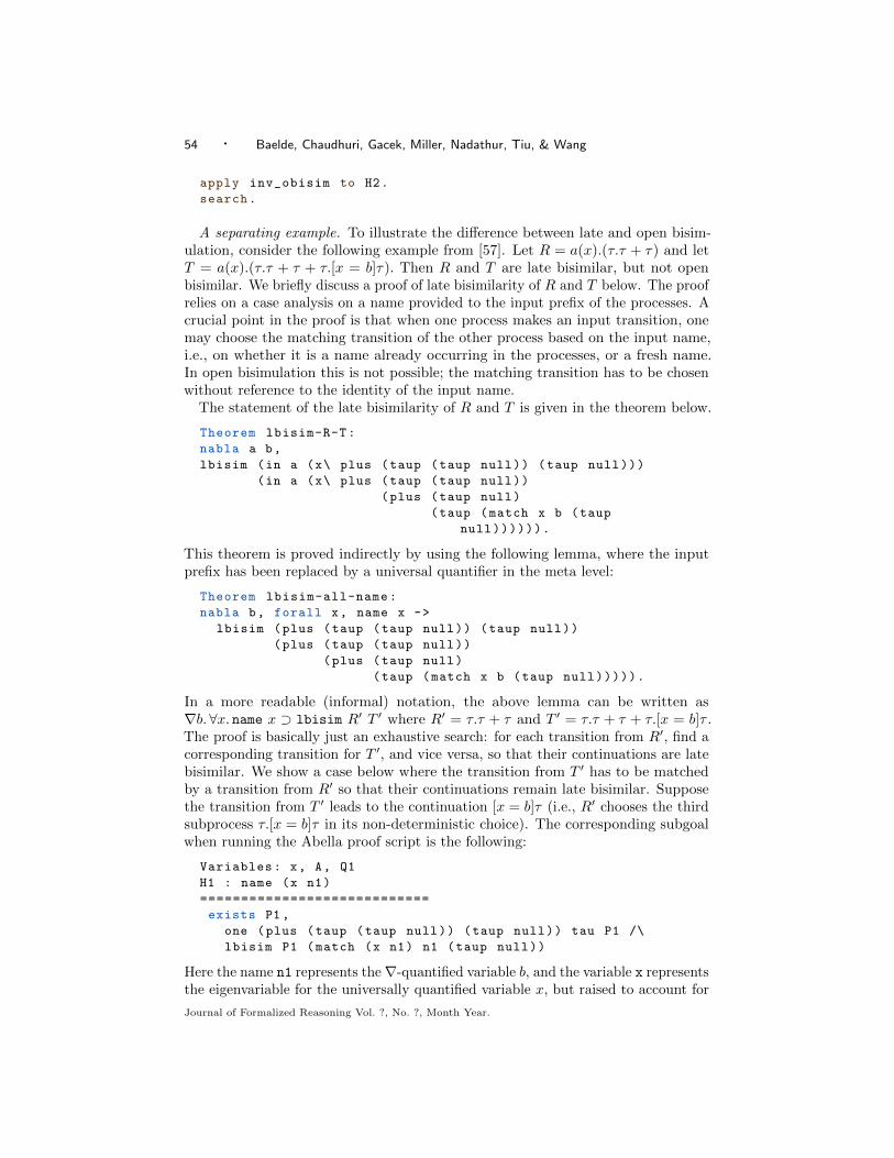
54 · Baelde, Chaudhuri, Gacek, Miller, Nadathur, Tiu, & Wang
apply inv_obisim to H2.
search.
A separating example. To illustrate the difference between late and open bisim-ulation, consider the following example from [57]. Let R = a(x).(τ.τ + τ) and letT = a(x).(τ.τ + τ + τ.[x = b]τ). Then R and T are late bisimilar, but not openbisimilar. We briefly discuss a proof of late bisimilarity of R and T below. The proofrelies on a case analysis on a name provided to the input prefix of the processes. Acrucial point in the proof is that when one process makes an input transition, onemay choose the matching transition of the other process based on the input name,i.e., on whether it is a name already occurring in the processes, or a fresh name.In open bisimulation this is not possible; the matching transition has to be chosenwithout reference to the identity of the input name.
The statement of the late bisimilarity of R and T is given in the theorem below.
Theorem lbisim-R-T:
nabla a b,
lbisim (in a (x\ plus (taup (taup null)) (taup null)))
(in a (x\ plus (taup (taup null))
(plus (taup null)
(taup (match x b (taup
null)))))).
This theorem is proved indirectly by using the following lemma, where the inputprefix has been replaced by a universal quantifier in the meta level:
Theorem lbisim-all-name:
nabla b, forall x, name x ->
lbisim (plus (taup (taup null)) (taup null))
(plus (taup (taup null))
(plus (taup null)
(taup (match x b (taup null))))).
In a more readable (informal) notation, the above lemma can be written as∇b.∀x. name x ⊃ lbisim R′ T ′ where R′ = τ.τ + τ and T ′ = τ.τ + τ + τ.[x = b]τ .The proof is basically just an exhaustive search: for each transition from R′, find acorresponding transition for T ′, and vice versa, so that their continuations are latebisimilar. We show a case below where the transition from T ′ has to be matchedby a transition from R′ so that their continuations remain late bisimilar. Supposethe transition from T ′ leads to the continuation [x = b]τ (i.e., R′ chooses the thirdsubprocess τ.[x = b]τ in its non-deterministic choice). The corresponding subgoalwhen running the Abella proof script is the following:
Variables: x, A, Q1
H1 : name (x n1)
============================
exists P1 ,
one (plus (taup (taup null)) (taup null)) tau P1 /\
lbisim P1 (match (x n1) n1 (taup null))
Here the name n1 represents the∇-quantified variable b, and the variable x representsthe eigenvariable for the universally quantified variable x, but raised to account for
Journal of Formalized Reasoning Vol. ?, No. ?, Month Year.

Abella: A System for Reasoning about Relational Specifications · 55
its relative scoping with respect to n1. The variable A, which has been instantiatedto tau, represents the action taken by process R′ and the variable Q1, instantiatedto (match (x n1) n1 (taup null)), represents the continuation of T ′.
The matching transition from R′ in this case depends on the value of x. If x = b,then [x = b]τ is equivalent to τ , so in this case the transition from R′ needs to bederived from the first subprocess in its non-deterministic choice, i.e., the process τ.τ .If x 6= b, then [x = b]τ is equivalent to the null process, so in this case we choose thesecond subprocess of R′ to drive the transition. The continuations of R′ for thesecases are τ and 0, respectively.
lbisim-all-name < case H1.
Subgoal 4.2.2.1:
Variables: x, A, Q1
============================
exists P1 ,
one (plus (taup (taup null)) (taup null)) tau P1 /\
lbisim P1 (match n2 n1 (taup null))
Subgoal 4.2.2.2 is:
exists P1 ,
one (plus (taup (taup null)) (taup null)) tau P1 /\
lbisim P1 (match n1 n1 (taup null))
In the first subgoal, the variable (x n1) is instantiated with a new nominalconstant n2. This subgoal can be simplified by instantiating P1 with null, followedby the tactics split and search, resulting in a new subgoal:
Variables: x, A, Q1
============================
lbisim null (match n2 n1 (taup null))
This can then be proved by a simple exhaustive search.The second subgoal (4.2.2.2) can be simplified by instantiating P1 with (taup
null), followed by the tactics split and search. These reduce the subgoal to
Variables: x, A, Q1
============================
lbisim (taup null) (match n1 n1 (taup null))
which can be proved by an exhaustive search.Let us now look at why open bisimilarity does not hold between R and T . As
with late bisimilarity, proving obisim R T in this case reduces to proving a lemmasimilar to lbisim-all-name, but without assuming name x:
Theorem obisim-for-all:
nabla b, forall x,
obisim (plus (taup (taup null)) (taup null))
(plus (taup (taup null))
(plus (taup null)
(taup (match x b (taup null))))).
To prove this lemma, we would have a similar subgoal as Subgoal 4.4.2 above,but without assuming name (x n1):
Journal of Formalized Reasoning Vol. ?, No. ?, Month Year.

56 · Baelde, Chaudhuri, Gacek, Miller, Nadathur, Tiu, & Wang
Variables: x
============================
exists P1 ,
one (plus (taup (taup null)) (taup null)) tau P1 /\
obisim P1 (match (x n1) n1 (taup null))
The only way the proof search could proceed is to instantiate P1 with a process.There are two choices for the instantiations of P1 that would satisfy the first conjunctin the goal: (taup null) or null. If we take the first choice, we end up having toprove:
Variables: x
============================
obisim (taup null) (match (x n1) n1 (taup null))
Since x is an eigenvariable, if this subgoal were provable, any instance of it wouldalso be provable. In particular, the instance
obisim (taup null) (match n2 n1 (taup null))
where x is instantiated to x\n2, for some fresh nominal constant n2, would also beprovable. Since match n2 n1 (taup null) is (open/late) bisimilar to null, thissubgoal would not be provable. So we are left with the only other choice for P1, i.e.,the process null. But in this case, we would have to prove the subgoal:
Variables: x
============================
obisim null (match (x n1) n1 (taup null))
If this were provable, then obisim null (match n1 n1 (taup null)) would alsobe provable, by letting x to be y\y. But match n1 n1 (taup null) is bisimilar to(taup null), which is not bisimilar to null, so this subgoal would not be provableeither. Having exhausted all the choices for the instantiation of P1 we conclude thatthe original goal obisim R T is not provable.
The reader may wonder whether the above argument of non-provability of obisimR T could be internalized as a proof within Abella of the negation of obisim R T.This is unfortunately not the case. The reason has to do with the shallow embeddingapproach we have taken in formalizing open bisimulation. To prove the negationof obisim R T, we would have to reason about non-provability of continuationsof obisim R T under some respectful substitutions, and one would need to reasonexplicitly about such substitutions and their effect on bisimilarity. If we were touse a deep embedding, e.g., by formalizing explicitly the notion of distinctions andrespectful substitutions, such a proof may be possible.
8. THE TWO-LEVEL LOGIC APPROACH
As Sections 4, 5, 6, and 7 have illustrated, Abella has sophisticated support forreasoning about relations. This makes it particularly well suited for specificationsin the structural operational semantics style [54, 55] that use inductively definedrelations to specify computational behavior. However, Abella’s definitions must bestratified : the defined predicates cannot be used negatively in their own definitions.This limitation means that when specifying relations that induct on the structure of
Journal of Formalized Reasoning Vol. ?, No. ?, Month Year.

Abella: A System for Reasoning about Relational Specifications · 57
higher-order λ-terms used in λ-tree syntax, we cannot rely on hypothetical reasoning,as is done in systems such as λProlog [39] or Twelf [50]. Instead, we use anexplicit context Gamma of typing assumptions, as we have illustrated in Sections 6.2and 7.2. Such definitions, where an explicit context argument has been added, areaccompanied by an obvious problem: the meta-theoretic properties of such listsof assumptions have to be established explicitly by the user. For instance, for theversion of the of predicate from Section 6.2, we had to manually prove the of_inst
theorem by induction. Moreover, we often need to know that the proof of this kindof theorem is height-preserving. This height is not part of the obvious encoding ofthe predicate in G. To make it available in constructing inductive proofs, we wouldneed to extend the definition of the of predicate with an extra height parameter,together with its associated assumptions using is_nat (cf. Section 2.2). In additionto the extra complexity in the definitions and theorems, we would also need tomaintain these proofs throughout the evolution of the system being specified. And,finally, after we are done with one definition, we would need to do everything againfor a different definition with different kinds of hypotheses.
The two level logic approach [23, 35] is a way to alleviate this tedium of meta-theoretic reasoning by defining a canonical hypothetical inductive definition thatcan capture a wide spectrum of other definitions using hypothetical reasoning.Specifically, it uses the logic of hereditary Harrop formulas [39, Chapter 3] as aspecification logic where hypothetical definitions are specified using higher-orderclauses that may be freely extended without needing to revisit any meta-theorems.8
This modularity is achieved by encoding derivability of specification logic sequentsas an inductive definition in G, for which the meta-theory is proved once and for all,as we have done in Section 7.2.
The following are some of the main benefits of the two-level logic approach.
(1) The specification logic operates under an open world assumption, where newclauses can always be added without affecting derivability in the specificationlogic. The reasoning logic (G), on the other hand, retains its closed worldreading where the collection of clauses of an inductive relation are fixed andstable with respect to unfolding. In particular, the reasoning logic can reasonabout both derivability and non-derivability of specification logic formulas andsequents, whereas the specification logic itself has no negation connective.9
(2) Because all specifications are factored through a common specification logic, themeta-theoretic properties of the specifications are obtained via the meta-theoryof the specification logic itself. Indeed, since this meta-theory is fixed andpredictable, the tactics of the reasoning logic can often be optimized to utilizethe meta-theorems on the fly and without user direction. This is commonlysummarized by the slogan “substitution lemmas for free.”
(3) Although not a property of the two-level logic approach as such, the specificationlogic of hereditary Harrop formulas underlies the λProlog programming language.
8To be more accurate, the two-level logic approach can be used with any specification logic that has
certain meta-theoretic properties. For example, the approach is easily adapted to linear logic [35]or intuitionistic dependent type theory [16, 17, 61, 62] as the specification logic.9Note that, in a situation where new clauses can always be added, there is no sensible way to
prove ¬A, as any such proof will not survive extensions with clauses that prove A.
Journal of Formalized Reasoning Vol. ?, No. ?, Month Year.

58 · Baelde, Chaudhuri, Gacek, Miller, Nadathur, Tiu, & Wang
Thus, specifications can be directly executed using λProlog implementationssuch as Teyjus [56]. We can thus prove properties of specifications that, undera different view, actually constitute code.
We will introduce the two-level logic approach in stages, starting with the simplecase of Horn clause specifications and moving on to more complex higher-orderspecifications.
8.1 Horn clause specifications
Let us begin with a simple Horn clause specification of appending lists. To avoidnamespace collisions with the definitions in Section 4.2 we will use the base typesi (for individuals) and ilist for lists of individuals. The appending operation onilists will then be given as a specification-level relation iappend; more concretely,the specification logic has a type o of formulas, and iappend will have type ilist
-> ilist -> ilist -> o. Following λProlog conventions, these specification typesare defined in a signature file (that must have extension .sig), here ilist.sig:
sig ilist.
kind i type.
type a,b,c i. % some individuals
kind ilist type.
type inil ilist.
type icons i -> ilist -> ilist.
type iappend ilist -> ilist -> ilist -> o.
The clauses defining iappend are given in a corresponding module file (with extension.mod), here ilist.mod:
module ilist.
iappend inil L L.
iappend (icons X L) K (icons X M) :-
iappend L K M.
These files follow standard λProlog syntactic conventions of capitalizing the univer-sally quantified variables in a clause and using :- to separate the head of a clausefrom its body.
In Abella, this specification can be imported by means of the Specification
top-level command.
Abella < Specification "ilist".
Reading specification "ilist"
If this command is used, it must be the first one in the run of Abella, because everyrun of Abella is parameterized on a given specification (which may be empty). Theeffect of this command is to transport the specification signature, without change orinterpretation, into the type system of Abella’s reasoning logic. In other words, it isas if the following top-level commands were submitted to Abella.
Kind i type.
Type a, b, c i.
Kind ilist type.
/* ... and so on */
Journal of Formalized Reasoning Vol. ?, No. ?, Month Year.

Abella: A System for Reasoning about Relational Specifications · 59
The clauses from the corresponding .mod are also loaded into memory. (The precisenature of the inclusion of the clauses will be made clear in the next subsection.)
To gain access to derivations in the specification logic, Abella uses the notation{F}, where F is a specification logic formula (i.e., a term of type o), to assert that Fis derivable in the specification logic from the loaded clauses. It is possible to useAbella as a logic programming interpreter by using the top-level Query commandto search for derivations. Here is an example:
Abella < Query {iappend L K (icons a (icons b inil))}.
Found solution:
L = inil
K = icons a (icons b inil)
Found solution:
L = icons a inil
K = icons b inil
Found solution:
L = icons a (icons b inil)
K = inil
No more solutions.
The logic programming interpreter executes the query by interpreting the capitalizedidentifiers as logic variables, and outputs their substitutions for each successfulsolution. It does not terminate if there are infinitely many solutions. This interpreteris provided primarily as a debugging aid; it is not competitive with sophisticatedλProlog execution frameworks.
The more interesting way to use such specifications is to prove properties aboutthem. As a first example, let us prove that iappend is deterministic: given two listsL and K, there is always at most one M for which iappend L K M may be derived inthe specification logic. We can write this theorem statement fairly directly in thereasoning logic:
Theorem iappend_det3 : forall L K M1 M2 ,
{iappend L K M1} -> {iappend L K M2} -> M1 = M2.
Note that the computational behavior of iappend is stated here in terms of whatcan be derived in the specification logic from the clauses defining this predicate. Theproof of this theorem will accordingly be based on an analysis of such derivations.Informally, we reason by induction on the height of one of the antecedent derivations,such as the first one:
iappend_det3 < induction on 1. intros.
Variables: L K M1 M2
IH : forall L K M1 M2, {iappend L K M1}* ->
{iappend L K M2} -> M1 = M2
H1 : {iappend L K M1}@
H2 : {iappend L K M2}
============================
M1 = M2
Journal of Formalized Reasoning Vol. ?, No. ?, Month Year.

60 · Baelde, Chaudhuri, Gacek, Miller, Nadathur, Tiu, & Wang
Observe that the the inductive restrictions @ and * (cf. Section 5) are attached tothe {} predicates. The hypotheses H1 and H2 are now available for case-analysis;whenever we use a clause for the iappend predicate in this analysis, the accompanying@ annotation (if any) is reduced to a *. For didactic purposes, let us turn on theinstantiations flag so that we can see how the variables get instantiated duringcase-analysis.
Set instantiations on.
Case-analysis of H1 yields two subgoals, one for each clause of iappend. The firstsubgoal results from matching the first clause:
iappend_det3 < case H1.
Variables: M1 M2
L <-- inil
K <-- M1
IH : forall L K M1 M2, {iappend L K M1}* ->
{iappend L K M2} -> M1 = M2
H2 : {iappend inil M1 M2}
============================
M1 = M2
We can then case-analyze H2 to also instantiate M2 with M1 which reduces the subgoalto a trivial equality (that can be finished with search).
iappend_det3 < case H2.
Variables: M2
L <-- inil
K <-- M2
M1 <-- M2
IH : forall L K M1 M2, {iappend L K M1}* ->
{iappend L K M2} -> M1 = M2
============================
M2 = M2
The second subgoal results from matching the second clause of iappend:
Variables: K M2 M L1 X
L <-- icons X L1
M1 <-- icons X M
IH : forall L K M1 M2, {iappend L K M1}* ->
{iappend L K M2} -> M1 = M2
H2 : {iappend (icons X L1) K M2}
H3 : {iappend L1 K M}*
============================
icons X M = M2
Note here that the inductive restriction on H3 has reduced from that of H1. Theproof proceeds by case-analysis of H2 which also instantiates M2 to icons X M3 (fora new variable M3) to yield:
iappend_det3 < case H2.
Journal of Formalized Reasoning Vol. ?, No. ?, Month Year.

Abella: A System for Reasoning about Relational Specifications · 61
Variables: K M L1 X M3
L <-- icons X L1
M1 <-- icons X M
M2 <-- icons X M3
IH : forall L K M1 M2, {iappend L K M1}* ->
{iappend L K M2} -> M1 = M2
H3 : {iappend L1 K M}*
H4 : {iappend L1 K M3}
============================
icons X M = icons X M3
Since the inductive restrictions now match, we can apply IH to H3 H4 to getM = M3, from which the conclusion follows trivially.
In effect, the theorem proceeds as if Abella had the following inductive definitionat the reasoning level (although the syntax is invalid).
Define {iappend} : ilist -> ilist -> ilist -> prop by
{iappend inil L L} ;
{iappend (icons X L) K (icons X M)} := {iappend L K M}.
The correspondence is strong; if we turn the above invalid syntax into an actualdefinition iappend_m (m for meta):
Define iappend_m : ilist -> ilist -> ilist -> prop by
iappend_m inil L L ;
iappend_m (icons X L) K (icons X M) := iappend_m L K M.
then we can prove both the following theorems by a simple induction (indeed, theproofs are identical).
Theorem spec_meta : forall L K M,
{iappend L K M} -> iappend_m L K M.
Theorem meta_spec : forall L K M,
iappend_m L K M -> {iappend L K M}.
More generally, for Horn clause specifications it is a matter of taste whether touse the specification or the reasoning logic from the perspective of proving meta-theorems. Of course, if we use the specification logic for such specifications, we havethe benefit of being able to execute them using an λProlog implementation; thusour meta-theorems state properties of actual code.
Before proceeding further, the reader is encouraged to attempt proving the follow-ing meta-theorems to get a feel for reasoning about specification logic derivations.
Theorem iappend_det2 : forall L K1 K2 M,
{iappend L K1 M} -> {iappend L K2 M} -> K1 = K2.
Theorem iappend_assoc : forall L K M LK KM N1 N2 ,
{iappend L K LK} -> {iappend K M KM} ->
{iappend LK M N1} -> {iappend L KM N2} -> N1 = N2.
8.2 Hereditary Harrop specifications
The truly interesting applications of the two-level logic approach arise when specifica-tions go beyond Horn clauses by employing universal quantification and implications
Journal of Formalized Reasoning Vol. ?, No. ?, Month Year.

62 · Baelde, Chaudhuri, Gacek, Miller, Nadathur, Tiu, & Wang
Abstract Concrete Precedence/Associativity
Formulas (F,G, . . . )Atomic formulas p m1 · · · mn p M1 ... Mn 5, left
Implication F ⇒ G F => G 4, right
G <= F 3, leftUniversal quantification Πx. F pi x\ F 1
Πx:τ. F pi (x:T)\ F 1
(parentheses optional)Conjunction F &G F & G 2, left
Truth tt (no concrete syntax)
Clauses
p m1 · · · mn︸ ︷︷ ︸head
. stands for Π ~X. (p m1 · · · mn)
p m1 · · · mn︸ ︷︷ ︸head
:- F1, . . . ,Fk︸ ︷︷ ︸body
. stands for Π ~X. (Fk ⇒ · · · ⇒ F1 ⇒ p m1 · · · mn)
(where ~X are the free capitalized identifiers in the clause)
Fig. 5: Concrete Syntax for hereditary Harrop formulas and specification logic clauses.
in the bodies of clauses. Such specifications are particularly apt for λ-tree syntax,where descending under a λ-abstraction is mirrored by introducing a universallyquantified variable to stand for the bound variable in the body of the clause, andwhere associated properties of that variable are encoded as extra antecedents in animplication. This style specification is best illustrated with an example, for whichwe revisit the simply typed λ-calculus from Section 6.4, but place the clauses in thespecification logic. The signature is:
sig stlc.
kind ty type.
type a ty.
type arr ty -> ty -> ty.
kind tm type.
type app tm -> tm -> tm.
type abs ty -> (tm -> tm) -> tm.
We will encode the typing relation using the specification logic predicate of whosetype is given by the following declaration.
type of tm -> ty -> o.
Recall that o is the type of specification logic formulas. These formulas arecomposed of atomic formulas built out of predicates such as iappend and of, andthe connectives of the logic of hereditary Harrop formulas defined in Section 7.2.Table 5 summarizes the concrete syntax of specification formulas and clauses thatis supported by Abella. Note that this concrete syntax is only a fragment of thefull λProlog language; in particular, Abella’s specification logic is simply typed,lacks disjunction and existential quantification, and only supports atomic heads inclauses.
Journal of Formalized Reasoning Vol. ?, No. ?, Month Year.
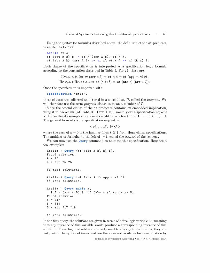
Abella: A System for Reasoning about Relational Specifications · 63
Using the syntax for formulas described above, the definition of the of predicateis written as follows.
module stlc.
of (app M N) B :- of M (arr A B), of N A.
of (abs A R) (arr A B) :- pi x\ of x A => of (R x) B.
Each clause of the specification is interpreted as a specification logic formulaaccording to the convention described in Table 5. For of, these are:
Πm,n, a, b. (of m (arr a b)⇒ of n a⇒ of (app m n) b) ,
Πr, a, b. ((Πx. of x a⇒ of (r x) b)⇒ of (abs r) (arr a b)) .
Once the specification is imported with
Specification "stlc".
these clauses are collected and stored in a special list, P, called the program. Wewill therefore use the term program clause to mean a member of P.
Since the second clause of the of predicate contains an embedded implication,using it to backchain {of (abs R) (arr A B)} would yield a specification sequentwith a localized assumption for a new variable x, written {of x A |- of (R x) B}.The general form of such a specification sequent is:
{ F1, . . . , Fn |- G }
where the case of n = 0 is the familiar form { G } from Horn clause specifications.The multiset of formulas to the left of |- is called the context of the sequent.
We can now use the Query command to animate this specification. Here are afew examples:
Abella < Query {of (abs A x\ x) B}.
Found solution:
A = ?5
B = arr ?5 ?5
No more solutions.
Abella < Query {of (abs A x\ app x x) B}.
No more solutions.
Abella < Query nabla x,
{of x (arr A B) |- of (abs A y\ app x y) D}.
Found solution:
A = ?17
B = ?19
D = arr ?17 ?19
No more solutions.
In the first query, the solutions are given in terms of a free logic variable ?5, meaningthat any instance of this variable would produce a corresponding instance of thissolution. These logic variables are merely used to display the solutions; they arenot part of the syntax of terms and are therefore not available for manipulation by
Journal of Formalized Reasoning Vol. ?, No. ?, Month Year.

64 · Baelde, Chaudhuri, Gacek, Miller, Nadathur, Tiu, & Wang
users. The second query asks about the term λx. (x x) that is ill-typed, and Abellaresponds with no solutions. The third query contains a nabla-quantified variable x.The logic variables A, B, etc. are existentially quantified at an outermost scope, sothe solutions for them cannot depend on x.
It is instructive at this juncture to trace the derivation of the solution of the thirdquery step-by-step.
Theorem explore : forall A B, nabla x,
{of x (arr A B) |- of (abs A y\ app x y) (arr A B)}.
intros.
This brings us to:
Variables: A B
============================
{of n1 (arr A B) |- of (abs A (y\ app n1 y)) (arr A B)}
We can now match the goal of (abs A (y\ app n1 y)) (arr A B) against thehead of the clause for abs in stlc.mod, which instantiates the variable R in thehead of the clause with y\ app n1 y. The resulting goal10 should therefore be:
Variables: A B
============================
{of n1 (arr A B) |- pi z\ of z A => of ((y\ app n1 y) z) B}
However, this goal is not in a reduced form in the sense of M from Section 7.2.Abella performs this goal reduction automatically, promoting pi-bound variables tonabla-bound variables, and transferring antecedents of => to the context. Abellathen also normalizes β-redexes and introduces the new nabla-quantified variables.The result is:
Variables: A B
============================
{of n1 (arr A B), of n2 A |- of (app n1 n2) B}
At this point we can continue with the clause for app to obtain:
Variables: A B
============================
exists A1 ,
{of n1 (arr A B), of n2 A |- of n1 (arr (A1 n2 n1) B)}
/\ {of n1 (arr A B), of n2 A |- of n2 (A1 n2 n1)}
Observe that we now have two goals because the body of the of_app clause hastwo predicates. Moreover, this clause involves a variable in the body that does notoccur in the head, so the result of the unfold is to existentially quantify over thatvariable. The Query command was able to find a substitution for the variable, butin our case we can provide it explicitly.
explore < witness u\ w\ A.
10To achieve this in the proof, one would use the unfold tactic using the named clauses feature.We leave a discussion of named clauses out of this tutorial as this is a new and experimentalfeature, and is only rarely useful.
Journal of Formalized Reasoning Vol. ?, No. ?, Month Year.

Abella: A System for Reasoning about Relational Specifications · 65
Variables: A B
============================
{of n1 (arr A B), of n2 A |- of n1 (arr A B)}
/\ {of n1 (arr A B), of n2 A |- of n2 A}
The remainder of the proof is straightforward: in each conjunct, the goal is foundamong the assumptions, so the subgoal can be closed with search.
What we achieved with unfold on the conclusion we can also achieve with case
on a hypothesis of a {} predicate; however, instead of selecting a clause, the case
tactic exhaustively considers all possible derivations, producing a subgoal for eachpossibility. As an example, suppose we wish to show the negation of the second(unprovable) query above.
Theorem explore2 : forall A B,
{of (abs A x\ app x x) B} -> false.
Since there is only one possible clause to backchain (of_abs), the case H1 commandproduces:
explore2 < intros. case H1.
Variables: A B1
H2 : {of n1 A |- of (app n1 n1) B1}
============================
false
At this point, case H2 produces two subgoals, the first of which we will skip fornow. The second subgoal is:
explore2 < case H2. skip.
Variables: A B1 F
H3 : {of n1 A, [F n1] |- of (app n1 n1) B1}
H4 : member (F n1) (of n1 A :: nil)
============================
false
Here we see the backchaining sequent form that has the general shape:
{ F1, . . . , Fn, [F] |- A }
where A is restricted to atomic specification-level formulas.11 This sequent form is thedirect representation of backchaining sequents from Section 7.2. The two hypothesesH3 and H4 are precisely the two conjuncts for the clause for the goal reductionrelation red that appeals to the backchaining relation bch, which corresponds tothe rule bch of Figure 2. They also have a natural reading: F n1 must be a memberof the context (H4) that can be used to backchain (H3).
At this point, if we try to case-analyze H3, then the case tactic will abort becausethe exact form of F n1 is not yet known. The tactic needs to make a decision here: ifthe head of the backchained clause matches the goal, then the tactic should producefresh assumptions for the body of the clause; however, if the head does not match,
11See [70] for a full explanation of how proof in the specification logic is organized within Abella.
Journal of Formalized Reasoning Vol. ?, No. ?, Month Year.

66 · Baelde, Chaudhuri, Gacek, Miller, Nadathur, Tiu, & Wang
then the tactic should close the subgoal for being vacuous. Neither choice can bemade yet, since we don’t yet know the head of F n1. (Note that the head of a clausemust be an atomic formula.)
In order to obtain this information about the structure of F n1, we must considerH4. Note that in H4 we have left the specification logic sequent form {} and areperforming meta-reasoning directly on the form of the context. This is the firstpoint where we need to know how specification contexts are represented in thereasoning logic. Abella represents such contexts as lists of specification formulas(i.e., terms of type o) using the type olist with two constructors, nil and ::, withthe latter written infix. This list type comes equipped with a member predicate withthis definition:
Define member : o -> olist -> prop by
member X (X :: L) ;
member X (Y :: L) := member X L.
Case-analysis of H4 will therefore lead to two subgoals for the two definitionalclauses of member, one where F n1 = of n1 A and the other with a fresh hypothesismember (F n1) nil. This latter case is trivial, so let us consider the former subgoal:
explore2 < case H4.
Variables: A B1
H3 : {of n1 A, [of n1 A] |- of (app n1 n1) B1}
============================
false
At this point, the case tactic can finally take a decision on H3, since the backchainedclause has an atomic head. Indeed, the head actually does not match the goal, sincen1 does not unify with app n1 n1, so the subgoal is finished with case H3.
This leaves just the subgoal that we skipped earlier, which is:
Variables: A B1 A1
H3 : {of n1 A |- of n1 (arr (A1 n1) B1)}
H4 : {of n1 A |- of n1 (A1 n1)}
============================
false
Here, the proof can be finished with a similar argument as before, starting with acase-analysis of H3 or H4. We leave it to the reader as an exercise.
8.3 Dynamic context management
Let us now try to show that the of predicate defined in the previous subsectionis deterministic in its second argument, i.e., that each term has at most one type.Following the pattern of Section 8.1, we might write the theorem as:
Theorem of_det2 : forall M A1 A2 ,
{of M A1} -> {of M A2} -> A1 = A2.
Like with lists earlier, this theorem is proved by induction on one of the antecedents,such as the first one. If we attempt a direct induction, we will succeed for backchain-ing the program clause for applications. However, for abstractions, we will end upwith the following subgoal:
Journal of Formalized Reasoning Vol. ?, No. ?, Month Year.

Abella: A System for Reasoning about Relational Specifications · 67
Variables: B R A B1
IH : forall M A1 A2, {of M A1}* -> {of M A2} -> A1 = A2
H3 : {of n1 A |- of (R n1) B}*
H4 : {of n1 A |- of (R n1) B1}
============================
arr A B = arr A B1
The IH cannot be applied to H3 and H4, even though the inductive restrictionsmatch, because the IH only applies to sequents with empty contexts.
The primary issue here is that the contexts of specification sequents grow whenbackchaining clauses, so the of_det2 theorem is not general enough. To generalizeit, we need to quantify over the possible specification sequent contexts
Theorem of_det2 ’ : forall L M A1 A2 ,
{L |- of M A1} -> {L |- of M A2} -> A1 = A2.
Abella therefore allows specification sequents to have the following structure:
{ L,F1, . . . , Fn |- G }
or
{ L,F1, . . . , Fn, [F] |- A }
where L is a variable of type olist, F1, . . . , Fn, F,G are formulas, and A is anatomic formula. We sometimes call L the context variable; if it exists, it must beunique and must be the first listed element of the context. Abella does not supportmultiple context variables within the same {}.
Using this kind of quantification over contexts, the unprovable subgoal earliernow becomes:
Variables: L B R A B1
IH : forall L M A1 A2, {L |- of M A1}* ->
{L |- of M A2} -> A1 = A2
H3 : {L, of n1 A |- of (R n1) B}*
H4 : {L, of n1 A |- of (R n1) B1}
============================
arr A B = arr A B1
We can now apply IH to H3 H4 by instantiating the L in the IH with of n1 A
:: L. However, the proof is not yet complete, as we now have a new possibility forproving {L |- of M A1}: backchaining a member of L:
Variables: L M A1 A2 F
IH : forall L M A1 A2, {L |- of M A1}* ->
{L |- of M A2} -> A1 = A2
H2 : {L |- of M A2}
H3 : {L, [F] |- of M A1}*
H4 : member F L
============================
A1 = A2
The hypothesis H3 is not usable by the IH as it involves a backchaining sequent. Theonly remaining option is to proceed by case-analysis. However, as we saw earlierin the trace through a query, the case tactic cannot yet decide on H3 as it does
Journal of Formalized Reasoning Vol. ?, No. ?, Month Year.

68 · Baelde, Chaudhuri, Gacek, Miller, Nadathur, Tiu, & Wang
not know the head of the formula F. Unlike the trace earlier, though, there is noother way to discover the form of F, since all we know is that it is a member ofsome olist, without any further information on how that olist is built. Hence,this proof attempt for of_det2’ is doomed without further constraining L.
What do we know about L? Let us think back to why we needed L in the first place:we needed to reason about {of (abs A R) (arr A B)}, which in turn required usto reason about {of n1 A |- of (R n1) B}. Thus, the kinds of members that weneed in L must include elements such as of n1 A. More generally, to derive of M A,we would need to extend the context by assumptions about bound variables, whichare in turn represented by nominal constants. This means that the possible formsof L must include at least the following subset (for any k ≥ 0):
of n1 A1, of n2 A2, . . . , of nk Ak.
Let us therefore attempt to prove the theorem parsimoniously for only these kindsof contexts. We achieve this by writing an inductive definition ctx for recognizingsuch contexts.
Define ctx : olist -> prop by
ctx nil ;
nabla x, ctx (of x A :: L) := ctx L.
The first clause accounts for the possibility of the context being empty, as is thecase for a closed term, while the second clause extends an existing context by asingle assumption about of in the form indicated above. Note the use here of nablaat the head (cf. Section 6.4). It guarantees that the ∇-quantified x is fresh for A
and L, which are universally quantified over the entire definitional clause.We can now state an inductively provable form of the of_det2 theorem.
Theorem of_det2_lem : forall L M A1 A2 , ctx L ->
{L |- of M A1} -> {L |- of M A2} -> A1 = A2.
induction on 2. intros. case H2.
Let us walk through some of the cases of this proof. The first subgoal is forbackchaining a program clause for app, which yields the subgoal:12
Variables: L A1 A2 A N M1
H1 : ctx L
H3 : {L |- of (app M1 N) A2}
H4 : {L |- of M1 (arr A A1)}*
H5 : {L |- of N A}*
============================
A1 = A2
At this point, we can proceed by case-analysis on H3. Unlike the previous proofof of_det2, the case tactic here yields two subgoals for the two possibilities forbackchaining: the program clause for app or a member of L. The former subgoal isstraightforward and identical to what we have already encountered, but the lattersubgoal is novel:
12In these subgoals, the IH is suppressed unless needed to prevent repetition.
Journal of Formalized Reasoning Vol. ?, No. ?, Month Year.

Abella: A System for Reasoning about Relational Specifications · 69
Variables: L A1 A2 A N M1 F
H1 : ctx L
H4 : {L |- of M1 (arr A A1)}*
H5 : {L |- of N A}*
H6 : {L, [F] |- of (app M1 N) A2}
H7 : member F L
============================
A1 = A2
We are in a similar situation to what we have seen before, but now we have anadditional hypothesis H1 that constrains L. Indeed, we can prove the followinglemma about all members of L.
Define fresh : tm -> ty -> prop by
nabla x, fresh x A.
Theorem ctx_mem : forall L F,
ctx L -> member F L ->
exists X A, (F = of X A) /\ fresh X A.
(The proof of ctx_mem is left as an easy exercise.) Back in the proof of of_det2_lem,we can now apply ctx_mem to H1 H7 to get:
Variables: L A1 A2 A N M1 X A3
H1 : ctx L
H4 : {L |- of M1 (arr A A1)}*
H5 : {L |- of N A}*
H6 : {L, [of X A3] |- of (app M1 N) A2}
H7 : member (of X A3) L
H8 : fresh X A3
============================
A1 = A2
At this point, the head of the backchained clause in H6 is atomic, so we can usecase H6 to unify X with app M1 N and A3 with A2. This changes H8 to fresh (app
M1 N) A2, which is not derivable as app M1 N is not a nominal constant. Thus,case H8 closes this subgoal.
The next subgoal is the case for backchaining a program clause for abs:
Variables: L A2 B R A
H1 : ctx L
H3 : {L |- of (abs A R) A2}
H4 : {L, of n1 A |- of (R n1) B}*
============================
arr A B = A2
Like with app earlier, using case H3 will leave us with two subgoals, the first ofwhich is:
IH : forall L M A1 A2, ctx L -> {L |- of M A1}* ->
{L |- of M A2} -> A1 = A2
H1 : ctx L
H4 : {L, of n1 A |- of (R n1) B}*
H5 : {L, of n1 A |- of (R n1) B1}
Journal of Formalized Reasoning Vol. ?, No. ?, Month Year.

70 · Baelde, Chaudhuri, Gacek, Miller, Nadathur, Tiu, & Wang
============================
arr A B = arr A B1
Now, in order to use the IH, we would need to prove that ctx (of n1 A ::
L). Since this follows trivially from H1 by search, Abella allows a special formof the apply tactic with some arguments left unspecified; they are inferred andautomatically proved by Abella.
of_det2_lem < apply IH to _ H4 H5.
Variables: L R A B1
H1 : ctx L
H4 : {L, of n1 A |- of (R n1) B1}*
H5 : {L, of n1 A |- of (R n1) B1}
============================
arr A B1 = arr A B1
The other subgoal amounts to backchaining a member of L to derive H3:
Variables: L A2 B R A F
H1 : ctx L
H4 : {L, of n1 A |- of (R n1) B}*
H5 : {L, [F] |- of (abs A R) A2}
H6 : member F L
============================
arr A B = A2
Here, as before with app, we use the ctx_mem lemma to derive that F must be ofthe form of n1 A1, and therefore case H5 can decide that H5 is not derivable andhence the goal must be closed.
This leaves us with the final subgoal that defeated our earlier attempt forof_det2’:
Variables: L M A1 A2 F
H1 : ctx L
H3 : {L |- of M A2}
H4 : {L, [F] |- of M A1}*
H5 : member F L
============================
A1 = A2
Here, we can use ctx_mem with H1 and H5 to derive the structure of F, which lets usrefine the goal further.
of_det2_lem < apply ctx_mem to H1 H5. case H6. case H4.
Variables: L A2 A3
H1 : ctx (L n1)
H3 : {L n1 |- of n1 (A2 n1)}
H5 : member (of n1 A3) (L n1)
============================
A3 = A2 n1
Journal of Formalized Reasoning Vol. ?, No. ?, Month Year.

Abella: A System for Reasoning about Relational Specifications · 71
Now, if we proceed by case-analysis on H3, there are no program clauses to backchainas none of these clauses define typing for nominal constants. So, the sole possibilityis backchaining a member of L n1.
of_det2_lem < case H3.
Variables: L A2 A3 F1
H1 : ctx (L n1)
H5 : member (of n1 A3) (L n1)
H7 : {L n1 , [F1 n1] |- of n1 (A2 n1)}
H8 : member (F1 n1) (L n1)
============================
A3 = A2 n1
Once again, we can appeal to ctx_mem to refine the subgoal further.
of_det2_lem < apply ctx_mem to H1 H8. case H7. case H9.
Variables: L A3 A5
H1 : ctx (L n1)
H5 : member (of n1 A3) (L n1)
H8 : member (of n1 A5) (L n1)
============================
A3 = A5
We have now reduced the problem of showing uniqueness of typing to showinguniqueness of typing assumptions for variables. This is easy to show, since our ctxdefinition always extends L with typing assumptions with a fresh nominal constant,and hence every typing assumption for a nominal constant occurs at most once. Wecan prove this as a lemma by induction.
Theorem ctx_uniq : forall L X A1 A2 , ctx L ->
member (of X A1) L -> member (of X A2) L -> A1 = A2.
The proof is left as an exercise (hint: use the following lemma).
Theorem member_prune : forall L E, nabla (x:tm),
member (E x) L -> exists F, E = x\ F.
We are now finally able to close the subgoal above with backchain ctx_uniq
with X = n1, L = L n1. The reader is encouraged to now re-organize this proofto see that it requires a definition ctx of certain kinds of contexts, a lemma ctx_mem
characterizing members of such contexts, and a lemma ctx_uniq that such contextsassign types functionally. Once these lemmas are in place, proving the determinancyof typing (of_det2_lem) is straightforward and our original theorem of_det2 is atrivial corollary.
8.4 Exploiting the meta-theory of the specification logic
As mentioned in the preamble of Section 8, one of the main benefits of using aspecification logic is that its meta-theory is proved once and for all (cf. Section 7.2).The following three meta-theorems are the most commonly encountered forms.
Journal of Formalized Reasoning Vol. ?, No. ?, Month Year.

72 · Baelde, Chaudhuri, Gacek, Miller, Nadathur, Tiu, & Wang
Monotonicity. The statement of the monotonicity theorem is as follows.
forall L K G, (forall E, member E L -> member E K) ->
{L |- G} -> {K |- G}.
As explained in Section 7.2, this theorem subsumes weakening, contraction, andexchange. One interesting aspect of this theorem is that it is height-preserving: if{L |- G} has an inductive restriction, then applying this theorem should preservethe restriction on {K |- G}. This is justified in Section 7.2 by the use of the heightparameter to red and bch that is shown to be preserved by the monotonicity meta-theorem. As the apply tactic of Abella does not preserve inductive restrictions onarguments, a special monotone tactic is used instead. For hypotheses of the form:
H1 : {L |- G} or H1 : {L |- G} *
the invocation monotone H1 with K produces a corresponding new hypothesis
H2 : {K |- G} or H2 : {K |- G} *
as appropriate, and an additional subgoal to prove forall E, member E L ->
member E K. Like with all tactics, the search tactic is automatically attempted onthis subgoal.
Instantiation. Nominal constants that appear in a specification logic sequent maybe replaced by any arbitrary term using the following instantiation theorem.
forall L G t, (nabla x, {L x |- G x}) -> {L t |- G t}.
Note that this is not perfectly valid Abella syntax because the statement is parametricon the type of x. In other words, it is a polymorphic theorem. Moreover, just aswith monotonicity, this theorem can preserve inductive restrictions, as proved inSection 7.2. Abella uses a specialized inst tactic for this theorem; for hypothesesof the form:
H1 : {L |- G} or H1 : {L |- G} *
the invocation inst H1 with n1 = t produces a corresponding new hypothesis
H2 : [t/n1] {L |- G} or H2 : [t/n1] {L |- G} *
where [t/n1] stands for the capture-avoiding substitution of t for n1 in the specifi-cation sequent. (Note: this substitution operation is not legal Abella syntax, just anotation used here to describe the tactic.)
Cut. The final meta theorem corresponds to the use of cut-admissibility of thespecification logic:
forall L F G, {L |- F} -> {L, F |- G} -> {L |- G}.
For hypotheses of the form:
H1 : {L |- F}
H2 : {L, F |- G}
the invocation cut H2 with H1 produces a new hypothesis:
H3 : {L |- G}
Journal of Formalized Reasoning Vol. ?, No. ?, Month Year.

Abella: A System for Reasoning about Relational Specifications · 73
If the two premises H1 and H2 do not have a common context L, then both sequentsare first put in the least context that contains both premise contexts (by internallyappealing to the monotone tactic). However, this operation comes with a limitation:since Abella allows at most a single context variable in specification sequents, theleast upper bound (in the inclusion ordering) of two specification contexts may notexist if their context variables differ. In this case, the user must first appeal to theother meta-theorems or lemmas to ensure both premise sequents have a commoncontext variable.
All three meta-theoretic tactics can also be applied to backchaining sequents whenthe syntax permits it.
Example. As an illustration of the use of the meta-theoretic tactics, considersubject-reduction in the simply typed λ-calculus. We first define the (big step)evaluation relation eval that has this type signature:
type eval tm -> tm -> o.
and these program clauses:
eval (abs A R) (abs A R).
eval (app M N) V :- eval M (abs A R), eval (R N) V.
The theorem we wish to prove is:
Theorem subjred : forall M V A,
{of M A} -> {eval M V} -> {of V A}.
The proof proceeds by induction on the second antecedent. The case of abstractionsis straightforward. For applications, we are in the following subgoal:
Variables: V A N R A1 M1 A2
IH : forall M V A, {of M A} -> {eval M V}* -> {of V A}
H3 : {eval M1 (abs A1 R)}*
H4 : {eval (R N) V}*
H5 : {of M1 (arr A2 A)}
H6 : {of N A2}
============================
{of V A}
Here, we apply IH to H5 H3 followed by case-analysis of the resulting hypothesisabout abs A1 R to get:
Variables: V A N R M1 A2
IH : forall M V A, {of M A} -> {eval M V}* -> {of V A}
H3 : {eval M1 (abs A2 R)}*
H4 : {eval (R N) V}*
H5 : {of M1 (arr A2 A)}
H6 : {of N A2}
H8 : {of n1 A2 |- of (R n1) A}
============================
{of V A}
In order to use the IH with H4, we need to show {of (R N) A}. To get there fromH8, we first instantiate the n1 with N, and then cut with H6.
Journal of Formalized Reasoning Vol. ?, No. ?, Month Year.

74 · Baelde, Chaudhuri, Gacek, Miller, Nadathur, Tiu, & Wang
subjred < inst H8 with n1 = N. cut H9 with H6.
Variables: V A N R M1 A2
IH : forall M V A, {of M A} -> {eval M V}* -> {of V A}
H3 : {eval M1 (abs A2 R)}*
H4 : {eval (R N) V}*
H5 : {of M1 (arr A2 A)}
H6 : {of N A2}
H8 : {of n1 A2 |- of (R n1) A}
H9 : {of N A2 |- of (R N) A}
H10 : {of (R N) A}
============================
{of V A}
Now we can apply IH to H10 H4 and finish the proof.
8.5 General context relations
The ctx definition in Section 8.3 was tailored to the of predicate. For a differentpredicate that would extend the context in a different way, we would need a differentvariant of the ctx relation. This leads to an obvious question: what if we need toprove a property about two different relations? One option might be to try to provethis property in a context that contains both kinds of extensions, but this tends tomake the proofs needlessly complicated, with extraneous subgoals in nearly everycase to rule out impossible situations. A more scalable option offered by Abella’srather general definition mechanism is to use separate tailored contexts for thevarious predicates with an explicit link between the separate contexts.
Once again, this technique is best described in terms of an example. Supposewe wish to define a binary relation copy on terms such that copy M N recursivelyexamines the structure of M and recreates it in N. It has this type signature:
type copy tm -> tm -> o.
and these clauses:
copy (app M1 M2) (app N1 N2) :-
copy M1 N1 , copy M2 N2.
copy (abs A R1) (abs A R2) :-
pi x\ copy x x => copy (R1 x) (R2 x).
The theorem we are interested in proving is the following:
Theorem copy_exists : forall M A, {of M A} -> {copy M M}.
(In fact, the theorem is weaker than it can be because copy works as well for termsthat are ill-typed according to of, but we ignore this issue as the example is mainlyused to illustrate a technique.)
Now, Section 8.3 should already have made it clear that we cannot hope to provethe copy_exists theorem directly by induction. Instead, we will need to prove ageneralized lemma that allows for contexts in the two clauses. How should thesecontexts be characterized? We can examine the program clauses of the of and copy
predicates to observe that the context extensions used to derive of M A are indeed
Journal of Formalized Reasoning Vol. ?, No. ?, Month Year.

Abella: A System for Reasoning about Relational Specifications · 75
related to the those for copy M M. When the former has a context of the form:
of n1 A1, of n2 A2, . . . , of nk Ak,
then the latter must have a context of the form:
copy n1 n1, copy n2 n2, . . . , copy nk nk.
We can therefore define, inductively, a binary context relation ctx2 that characterizesboth contexts at the same time.
Define ctx2 : olist -> olist -> prop by
ctx2 nil nil ;
nabla x, ctx2 (of x A :: L) (copy x x :: K) := ctx2 L K.
The second definitional clause guarantees that x is fresh for A, L, and K. We can thenprove a generalized lemma using ctx2 that will have copy_exists as a corollary.
Theorem copy_exists_lem : forall L K M A, ctx2 L K ->
{L |- of M A} -> {K |- copy M M}.
We proceed by a straightforward induction on the second antecedent; here aresome of the interesting cases. For backchaining the program clause for abs, we havethe subgoal:
Variables: L K B R A1
IH : forall L K M A, ctx2 L K ->
{L |- of M A}* -> {K |- copy M M}
H1 : ctx2 L K
H3 : {L, of n1 A1 |- of (R n1) B}*
============================
{K |- copy (abs A1 R) (abs A1 R)}
Here, we can finish the goal by apply IH to _ H3; Abella constructs and provesthe omitted goal that ctx2 (of n1 A1 :: L) (copy n1 n1 :: K). The otherinteresting subgoal arises from backchaining a member of L.
Variables: L K M A F
IH : forall L K M A, ctx2 L K ->
{L |- of M A}* -> {K |- copy M M}
H1 : ctx2 L K
H3 : {L, [F] |- of M A}*
H4 : member F L
============================
{K |- copy M M}
Like in Section 8.3, to make progress we need to know something about the membersof L. We can prove a variant of ctx_mem directly with an identical proof.
Theorem ctx2_mem1 : forall L K F,
ctx2 L K -> member F L ->
exists X A, (F = of X A) /\ fresh X A.
Alternatively, we can project the binary relation on its first argument and reuse thectx_mem theorem.
Theorem ctx2_proj1 : forall L K, ctx2 L K -> ctx L.
Journal of Formalized Reasoning Vol. ?, No. ?, Month Year.

76 · Baelde, Chaudhuri, Gacek, Miller, Nadathur, Tiu, & Wang
Whichever option is taken, we will be left with the subgoal:
Variables: L K A2
H1 : ctx2 (L n1) (K n1)
H4 : member (of n1 A2) (L n1)
============================
{K n1 |- copy n1 n1}
The proof can finish if we only knew that member (copy n1 n1) (K n1), as thereis no program clause for copy for nominal constants. This requires a separate lemmashowing the relationship between the members of contexts related by ctx2. Its easyproof is left as an exercise.
Theorem ctx2_sync : forall K L X A, ctx2 L K ->
member (of X A) L -> member (copy X X) K.
8.6 Extended example: Transitivity of subtyping in system Fsub
Our examples until now have used only a single nested implication in the bodiesof program clauses, which does not fully exploit the significant expressive powerof higher-order specifications. As an extended example of the possibilities offeredby such specifications, we will give here a version of the proof of transitivity ofsubtyping for system Fsub, which is an extension of system F with subtyping andbounded polymorphism. System Fsub is described in more detail in [52, Chapter 26],and transitivity of subtyping in Fsub is problem 1a of the POPLMark challenge [4].
The types (written using T, S, . . . ) of system Fsub are built from type variables(written α, β, . . . ) using the following grammar.
T, S, . . . ::= α | > | T → S | ∀α≤T. S
The type > is the greatest element of the subtype relation ≤. For the boundedpolymorphic type ∀α≤T. S, valid instances can only be created for type argumentsthat are ≤ T . The bound variable can be freely α-varied.
The subtyping relation can be inductively specified using subtyping contexts (Γ),which are multisets of elements of the form α≤T . The subtyping judgment has theform Γ ` S ≤ T with the following inference rules.
Γ, α≤T ` α ≤ T Γ ` α ≤ αΓ ` α ≤ S Γ ` S ≤ T
Γ ` α ≤ T Γ ` T ≤ >
Γ ` T1 ≤ S1 Γ ` S2 ≤ T2
Γ ` (S1 → S2) ≤ (T1 → T2)
Γ ` T1 ≤ S1 Γ, α ≤ T1 ` S2 ≤ T2
Γ ` (∀α≤S1. S2) ≤ (∀α≤T1. T2)
In the final rule, by standard convention, we require that α is not free in Γ.In order to encode this as a specification in Abella, we have two possibilities. The
first is to have a separate syntactic class of type variables for which the first threesubtyping rules apply, but this forces us to reason about α-equivalence. The otherchoice is to use λ-tree syntax to get the α-equivalence (among other properties) forfree, but then the first three rules are difficult to encode as λ-tree syntax has nobuilt in mechanism to detect when something is a variable. Either option seems topresent difficulties for the encoding.
Fortunately, there is a third possibility, suggested in [51], of retaining an encodingin λ-tree syntax while using higher-order clauses to construct specialized instances
Journal of Formalized Reasoning Vol. ?, No. ?, Month Year.

Abella: A System for Reasoning about Relational Specifications · 77
of the first three variable rules whenever a new variable is introduced into thesubtyping context. The unscoped form of these three rules are then removed fromthe system. We therefore use the following type signature for the grammar of types(tp) and for the subtyping relation sub.
sig fsub.
kind tp type.
type top tp.
type arr tp -> tp -> tp.
type all tp -> (tp -> tp) -> tp.
type sub tp -> tp -> o.
As is standard in λ-tree syntax, we use λ-terms to depict binding, so the type∀α≤S. T would be encoded as all S (a\ T ).
The clauses for the sub relation are as follows.
module fsub.
sub T top.
sub (arr S1 S2) (arr T1 T2) :- sub T1 S1 , sub S2 T2.
sub (all S1 S2) (all T1 T2) :-
sub T1 S1 ,
pi a\
(pi u\ pi v\ sub a u => sub u v => sub a v) =>
sub a T1 =>
sub a a =>
sub (S2 a) (T2 a).
The first two clauses are straightforward translations of the corresponding inferencerules. The body of the third clause has embedded clauses defining transitivity andreflexivity of subtyping for the bound type variable, represented here with the boundvariable a, and the fact that it is ≤ T1. Note that the assumption
pi u\ pi v\ sub a u => sub u v => sub a v
is a Horn clause program which is specialized to the variable a but which can beused with arbitrary types u and v to derive the subtyping relationships for a bytransitivity. In other words, it computes the transitive closure of subtyping chainsbeginning with a. This third program clause of sub is therefore a third-order clause,as there are second-order formulas in its body.
To prove that the specified relation sub enjoys transitivity of subtyping amountsto proving the following theorem in Abella:
Theorem transitivity ’ : forall S T U,
{sub S T} -> {sub T U} -> {sub S U}.
However, there is a problem: the proof of the theorem is by induction on thestructure of the intermediate type T, which in Abella requires a separate definition,is_tp, as we have seen before. Since the syntax of types is itself untyped,13 we
13Types do not have any classifiers in system Fsub.
Journal of Formalized Reasoning Vol. ?, No. ?, Month Year.

78 · Baelde, Chaudhuri, Gacek, Miller, Nadathur, Tiu, & Wang
reuse the technique from Section 7.1 of defining the structure of types in an openfashion, using nominal constants to stand for the type variables.
Define is_tp : tp -> prop by
nabla x, is_tp x ;
is_tp top ;
is_tp (arr S T) := is_tp S /\ is_tp T ;
is_tp (all S T) := is_tp S /\ nabla x, is_tp (T x).
Then, the actual transitivity theorem we show is:
Theorem transitivity : forall S T U, is_tp T ->
{sub S T} -> {sub T U} -> {sub S U}.
Of course, to prove this theorem we need to generalize the statement to reasonabout the context extensions resulting from backchaining the program clauses of sub.Like we have already seen in earlier subsections, this requires a context definitionctx characterizing the extensions to the context.
Define ctx : olist -> prop by
ctx nil ;
nabla a, ctx ((sub a a) ::
(sub a T) ::
(pi u\ pi v\ sub a u => sub u v => sub a v)
:: L) :=
ctx L.
The second clause of ctx adds three new members to the context, corresponding tothe three antecedents of the main implication in the body of the second programclause of sub.
Although this definition is somewhat more complex than similar definitions inearlier subsections, theorems such as ctx_mem are still easily defined and proved.
Define name : tp -> prop by
nabla x, name x.
Define fresh : tp -> tp -> prop by
nabla x, fresh x T.
Theorem ctx_mem : forall L F,
ctx L -> member F L ->
exists A,
(F = sub A A /\ name A)
\/ (exists T, F = sub A T /\ fresh A T)
\/ (F = (pi u\ pi v\ sub A u => sub u v => sub A v)
/\ name A).
The proof is marginally more complex than proofs of similar theorems in earliersubsections but is nevertheless straightforward and left as an exercise.
We can now state and prove the strengthened transitivity theorem.
Theorem transitivity : forall L S T U,
ctx L -> is_tp T ->
{L |- sub S T} -> {L |- sub T U} -> {L |- sub S U}.
induction on 2. intros.
Journal of Formalized Reasoning Vol. ?, No. ?, Month Year.

Abella: A System for Reasoning about Relational Specifications · 79
At this juncture it would be tempting to continue with case H2 but this would havethe effect of enumerating all types, regardless of whether those types are relatedto S or not. Therefore, we instead proceed with case H3, which produces foursubgoals: three for the possible ways to backchain a program clause for sub andone for backchaining an element of L.
The first subgoal, produced by backchaining the first program clause for sub, is:14
Variables: L S U
H1 : ctx L
H2 : is_tp top @
H4 : {L |- sub top U}
============================
{L |- sub S U}
Here, our only option is to continue with case H4, which produces two subgoals: onefor the first program clause for sub (which is trivial), and the other for backchaininga member of L, which is:
Variables: L S U F
H1 : ctx L
H2 : is_tp top @
H4 : {L |- sub top U}
H5 : {L, [F] |- sub top U}
H6 : member F L
============================
{L |- sub S U}
Now, we can apply ctx_mem to H1 H6; each resulting subgoal would be vacuousbecause top cannot unify with a nominal constant.
The next overall subgoal is for the program clause of sub involves setting T
to arr T1 T2: the resulting argument is straightforward. After that, the mostinteresting subgoal involves binding T to all T1 T2, which yields:
Variables: L U T2 S2 T1 S1
H1 : ctx L
H2 : is_tp (all T1 T2) @
H4 : {L |- sub (all T1 T2) U}
H5 : {L |- sub T1 S1}
H6 : {L, (pi u\ pi v\ sub n1 u => sub u v => sub n1 v),
sub n1 T1 , sub n1 n1 |- sub (S2 n1) (T2 n1)}
============================
{L |- sub (all S1 S2) U}
Once again we start with case H4, which produces three subgoals, two of which aresimilar to the previous cases, and the third (after a case H2) is:
Variables: L T2 S2 T1 S1 T3 T4
H1 : ctx L
H5 : {L |- sub T1 S1}
H6 : {L, (pi u\ pi v\ sub n1 u => sub u v => sub n1 v),
sub n1 T1 , sub n1 n1 |- sub (S2 n1) (T2 n1)}
14Once again, the IH is suppressed unless relevant.
Journal of Formalized Reasoning Vol. ?, No. ?, Month Year.

80 · Baelde, Chaudhuri, Gacek, Miller, Nadathur, Tiu, & Wang
H7 : {L |- sub T4 T1}
H8 : {L, (pi u\ pi v\ sub n1 u => sub u v => sub n1 v),
sub n1 T4 , sub n1 n1 |- sub (T2 n1) (T3 n1)}
H9 : is_tp T1 *
H10 : is_tp (T2 n1) *
============================
{L |- sub (all S1 S2) (all T4 T3)}
From apply IH to H1 H9 H7 H5 we immediately have {L |- sub T4 S1}. There-fore, all that remains is to link S2 and T3, which, by the program clause for sub,requires showing:
{L, (pi u\ pi v\ sub n1 u => sub u v => sub n1 v),
sub n1 T4 , sub n1 n1 |- sub (S2 n1) (T3 n1)}
We can nearly get there by the IH applied to H6 and H8, except that their contextsdo not match: one has sub n1 T1 while the other has sub n1 T4. But, by H7, weknow that sub T4 T1, which by the embedded clause in the context of H8 shouldlet us derive sub n1 T1. We assert this fact, which Abella can easily prove.
transitivity_lem <
assert {(pi u\ pi v\ sub n1 u => sub u v => sub n1 v),
sub T4 T1 , sub n1 T4 |- sub n1 T1}.
Variables: L T2 S2 T1 S1 T3 T4
H1 : ctx L
H5 : {L |- sub T1 S1}
H6 : {L, (pi u\ pi v\ sub n1 u => sub u v => sub n1 v),
sub n1 T1 , sub n1 n1 |- sub (S2 n1) (T2 n1)}
H7 : {L |- sub T4 T1}
H8 : {L, (pi u\ pi v\ sub n1 u => sub u v => sub n1 v),
sub n1 T4 , sub n1 n1 |- sub (T2 n1) (T3 n1)}
H9 : is_tp T1 *
H10 : is_tp (T2 n1) *
H11 : {L |- sub T4 S1}
H12 : {(pi u\ pi v\ sub n1 u => sub u v => sub n1 v),
sub T4 T1 , sub n1 T4 |- sub n1 T1}
============================
{L |- sub (all S1 S2) (all T4 T3)}
We can then cut the assumption sub T4 T1 using H7, and use the result to cut theassumption sub n1 T1 out of H6, yielding the required sequent to use with the IH.
The final overall subgoal corresponds to backchaining a member of L to derive{L |- sub S T}:
Variables: L S T U F
H1 : ctx L
H2 : is_tp T @
H4 : {L |- sub T U}
H5 : {L, [F] |- sub S T}
H6 : member F L
============================
{L |- sub S U}
Journal of Formalized Reasoning Vol. ?, No. ?, Month Year.

Abella: A System for Reasoning about Relational Specifications · 81
We can use ctx_mem now to examine all the possibilities for F. Most cases areimmediate; the sole exception is:
Variables: L U T2
H1 : ctx (L n1)
H2 : is_tp T2 @
H4 : {L n1 |- sub T2 (U n1)}
H6 : member (sub n1 T2) (L n1)
============================
{L n1 |- sub n1 (U n1)}
We know that if sub n1 T2 is in L n1, then it must have been added together witha Horn clause for transitivity for n1 at the same time. In other words, we need thefollowing theorem.
Theorem ctx_sync : forall L A T,
ctx L -> member (sub A T) L ->
member (pi u\ pi v\ sub A u => sub u v => sub A v) L.
The proof is by induction on the first antecedent and left as an exercise as well.Appealing to it for the above subgoal gives us enough information about the contentsof L n1 to derive the goal.
The complete proof is shown in Figure 6.
Fig. 6: full proof of the transitivity of subtyping for system Fsub
Theorem transitivity : forall L S T U,
ctx L -> is_tp T ->
{L |- sub S T} -> {L |- sub T U} -> {L |- sub S U}.
induction on 2. intros. case H3.
% T = top
case H4.
search.
apply ctx_mem to H1 H6. case H7.
case H5. case H8.
case H5. case H8.
case H5. case H8.
% T = arr T1 T2
case H4.
search.
case H2.
apply IH to H1 H9 H7 H5.
apply IH to H1 H10 H6 H8.
search.
apply ctx_mem to H1 H8. case H9.
case H7. case H10.
case H7. case H10.
case H7. case H10.
Journal of Formalized Reasoning Vol. ?, No. ?, Month Year.

82 · Baelde, Chaudhuri, Gacek, Miller, Nadathur, Tiu, & Wang
% T = all T1 T2
case H4.
search.
case H2.
apply IH to H1 H9 H7 H5.
assert { (pi u\ pi v\ sub n1 u => sub u v => sub n1
v),
sub T4 T1 , sub n1 T4 |- sub n1 T1 }.
cut H12 with H7. cut H6 with H13.
apply IH to _ H10 H14 H8.
search.
apply ctx_mem to H1 H8. case H9.
case H7. case H10.
case H7. case H10.
case H7. case H10.
% backchain on a member of L
apply ctx_mem to H1 H6. case H7.
% sub a a
case H5. search.
% sub a T1
case H5. case H8. apply ctx_sync to H1 H6. search.
% pi u\ pi v\ sub a u => sub u v => sub a v
case H5. search.
9. FUTURE DIRECTIONS
Currently in Abella, only predicates can be inductively defined although it is oftenconvenient to view types as being inductively (or co-inductively) defined. In orderto treat induction on types, one must write a predicate that repeats the descriptionof the type and then reason inductively on that predicate. We are consideringextending Abella so that all types can be immediately treated as if they were givenby predicate definitions.
There have been a number of places in Section 8 where contexts were defined anda number of technical but shallow theorems about contexts needed to be proved.Given that contexts are generally rather simple structures, a variant of Abella hasbeen developed [59] in which contexts can be declared differently than as lists: suchspecialized declarations allow for many of the technical lemmas to be proved byautomatically produced proof scripts.
The core logic of Abella does not allow either predicate quantification or poly-morphic typing. Its notion of modules is also rather primitive. By reconsideringmodular construction of theorem (.thm) files, it might be possible to view predicate
Journal of Formalized Reasoning Vol. ?, No. ?, Month Year.

Abella: A System for Reasoning about Relational Specifications · 83
quantification and polymorphic typing as features of a module language instead of(more controversially) the target logic.
The specification logic used in the two-level logic approach described in Section 8is the intuitionistic logic of hereditary Harrop formulas. This choice is appealingsince it is an expressive and popular logic that appears within a number of systems,including λProlog, Isabelle, Minlog, and Twelf. The exact subset of logic andits concrete syntax were chosen so that it corresponds to an executable subsetof λProlog and the Teyjus system [56] can be used to automatically search forproofs in that logic. There are, however, other natural choices of specification logics.For example, an early paper on the two-level logic approach [35] illustrated someadvantages of using, instead, a linear logic programming language [30]. More recently,a variant of Abella has been designed [62] in which an additional specification logicusing the dependently typed λ-calculus LF co-exists with the current specificationlanguage [29]. A natural question for the future development of Abella is how far totake this idea: should Abella be made generic over arbitrary specification languages(in which case we would need to consider the question of how specification languagesare formally defined) and should it support multiple specifications, possibly indifferent languages, at the same time?
The Bedwyr [7, 72] model checking system is based on a subset of the logicunderlying Abella. Providing articulation between these two systems could provevaluable for several reasons. For example, Bedwyr’s automated search can provetheorems that simply require complete state explorations: writing a complete prooffor such exploration in Abella is possible in principle but tedious and impractical.Also, Bedwyr could make use of lemmas proved in Abella in order to make its searchmore effective: for example, searching for a winning strategy in some board gamecould benefit significantly if it was known that symmetric versions of a winningposition are also winning. This latter fact could, in principle, be proved in Abellaand imported into Bedwyr.
References
[1] J.-M. Andreoli. Logic programming with focusing proofs in linear logic. J. ofLogic and Computation, 2(3):297–347, 1992.
[2] A. W. Appel and A. P. Felty. Dependent types ensure partial correctness oftheorem provers. J. Funct. Program., 14(1):3–19, 2004.
[3] A. Avron, F. Honsell, I. A. Mason, and R. Pollack. Using typed lambda calculusto implement formal systems on a machine. Journal of Automated Reasoning,9:309–354, 1992.
[4] B. E. Aydemir, A. Bohannon, M. Fairbairn, J. N. Foster, B. C. Pierce, P. Sewell,D. Vytiniotis, G. Washburn, S. Weirich, and S. Zdancewic. Mechanized metathe-ory for the masses: The POPLmark challenge. In Theorem Proving in HigherOrder Logics: 18th International Conference, number 3603 in LNCS, pages50–65. Springer, 2005.
[5] D. Baelde. A linear approach to the proof-theory of least and greatest fixedpoints. PhD thesis, Ecole Polytechnique, Dec. 2008.
[6] D. Baelde. On the expressivity of minimal generic quantification. In A. Abeland C. Urban, editors, International Workshop on Logical Frameworks and
Journal of Formalized Reasoning Vol. ?, No. ?, Month Year.

84 · Baelde, Chaudhuri, Gacek, Miller, Nadathur, Tiu, & Wang
Meta-Languages: Theory and Practice (LFMTP 2008), number 228 in ENTCS,pages 3–19, 2008.
[7] D. Baelde, A. Gacek, D. Miller, G. Nadathur, and A. Tiu. The Bedwyr systemfor model checking over syntactic expressions. In F. Pfenning, editor, 21thConf. on Automated Deduction (CADE), number 4603 in LNAI, pages 391–397,New York, 2007. Springer.
[8] D. Baelde and G. Nadathur. Combining deduction modulo and logics offixed-point definitions. pages 105–114. IEEE Computer Society Press, June2012.
[9] Y. Bertot and P. Casteran. Interactive Theorem Proving and Program Develop-ment. Coq’Art: The Calculus of Inductive Constructions. Texts in TheoreticalComputer Science. Springer, 2004.
[10] K. Chaudhuri. The Focused Inverse Method for Linear Logic. PhD thesis,Carnegie Mellon University, Dec. 2006. Technical report CMU-CS-06-162.
[11] J. Cheney. Equivariant unification. J. of Automated Reasoning, 45(3):267–300,Dec. 2010.
[12] A. Church. A formulation of the simple theory of types. J. of Symbolic Logic,5:56–68, 1940.
[13] N. G. de Bruijn. Lambda calculus notation with nameless dummies, a toolfor automatic formula manipulation, with an application to the Church-Rossertheorem. Indagationes Mathematicae, 34(5):381–392, 1972.
[14] A. Felty. Transforming specifications in a dependent-type lambda calculus tospecifications in an intuitionistic logic. In G. Huet and G. D. Plotkin, editors,Logical Frameworks. Cambridge University Press, 1991.
[15] A. Felty and D. Miller. Specifying theorem provers in a higher-order logicprogramming language. In Ninth International Conference on AutomatedDeduction, number 310 in LNCS, pages 61–80, Argonne, IL, May 1988. Springer.
[16] A. Felty and D. Miller. Encoding a dependent-type λ-calculus in a logicprogramming language. In M. Stickel, editor, Proceedings of the 1990 Conferenceon Automated Deduction, volume 449 of LNAI, pages 221–235. Springer, 1990.
[17] A. Felty and A. Momigliano. Hybrid: A definitional two-level approach toreasoning with higher-order abstract syntax. J. of Automated Reasoning, 48:43–105, 2012.
[18] M. J. Gabbay and A. M. Pitts. A new approach to abstract syntax with variablebinding. Formal Aspects of Computing, 13:341–363, 2001.
[19] A. Gacek. A Framework for Specifying, Prototyping, and Reasoning aboutComputational Systems. PhD thesis, University of Minnesota, 2009.
[20] A. Gacek. Relating nominal and higher-order abstract syntax specifications. InProceedings of the 2010 Symposium on Principles and Practice of DeclarativeProgramming, pages 177–186. ACM, July 2010.
[21] A. Gacek, D. Miller, and G. Nadathur. Combining generic judgments withrecursive definitions. In F. Pfenning, editor, 23th Symp. on Logic in ComputerScience, pages 33–44. IEEE Computer Society Press, 2008.
Journal of Formalized Reasoning Vol. ?, No. ?, Month Year.

Abella: A System for Reasoning about Relational Specifications · 85
[22] A. Gacek, D. Miller, and G. Nadathur. Nominal abstraction. Information andComputation, 209(1):48–73, 2011.
[23] A. Gacek, D. Miller, and G. Nadathur. A two-level logic approach to reasoningabout computations. J. of Automated Reasoning, 49(2):241–273, 2012.
[24] G. Gentzen. Investigations into logical deduction. In M. E. Szabo, editor, TheCollected Papers of Gerhard Gentzen, pages 68–131. North-Holland, Amsterdam,1935. Translation of articles that appeared in 1934-35. Collected papers appearedin 1969.
[25] J.-Y. Girard. A fixpoint theorem in linear logic. An email posting to the mailinglist [email protected], Feb. 1992.
[26] J. Hannan. Extended natural semantics. J. of Functional Programming,3(2):123–152, Apr. 1993.
[27] J. Hannan and D. Miller. From operational semantics to abstract machines.Mathematical Structures in Computer Science, 2(4):415–459, 1992.
[28] J. Hannan and F. Pfenning. Compiler verification in LF. In 7th Symp. onLogic in Computer Science, Santa Cruz, California, June 1992. IEEE ComputerSociety Press.
[29] R. Harper, F. Honsell, and G. Plotkin. A framework for defining logics. Journalof the ACM, 40(1):143–184, 1993.
[30] J. Hodas and D. Miller. Logic programming in a fragment of intuitionisticlinear logic. Information and Computation, 110(2):327–365, 1994.
[31] G. Huet. A unification algorithm for typed λ-calculus. Theoretical ComputerScience, 1:27–57, 1975.
[32] G. Huet and B. Lang. Proving and applying program transformations expressedwith second-order patterns. Acta Informatica, 11:31–55, 1978.
[33] C. Liang and D. Miller. Focusing and polarization in linear, intuitionistic, andclassical logics. Theoretical Computer Science, 410(46):4747–4768, 2009.
[34] R. McDowell and D. Miller. Cut-elimination for a logic with definitions andinduction. Theoretical Computer Science, 232:91–119, 2000.
[35] R. McDowell and D. Miller. Reasoning with higher-order abstract syntax in alogical framework. ACM Trans. on Computational Logic, 3(1):80–136, 2002.
[36] R. McDowell, D. Miller, and C. Palamidessi. Encoding transition systems insequent calculus. Theoretical Computer Science, 294(3):411–437, 2003.
[37] D. Miller. A logic programming language with lambda-abstraction, functionvariables, and simple unification. J. of Logic and Computation, 1(4):497–536,1991.
[38] D. Miller and G. Nadathur. A logic programming approach to manipulatingformulas and programs. In S. Haridi, editor, IEEE Symposium on LogicProgramming, pages 379–388, San Francisco, Sept. 1987.
[39] D. Miller and G. Nadathur. Programming with Higher-Order Logic. CambridgeUniversity Press, June 2012.
[40] D. Miller, G. Nadathur, F. Pfenning, and A. Scedrov. Uniform proofs as afoundation for logic programming. Annals of Pure and Applied Logic, 51:125–157, 1991.
Journal of Formalized Reasoning Vol. ?, No. ?, Month Year.

86 · Baelde, Chaudhuri, Gacek, Miller, Nadathur, Tiu, & Wang
[41] D. Miller and C. Palamidessi. Foundational aspects of syntax. ACM ComputingSurveys, 31, Sept. 1999.
[42] D. Miller and A. Tiu. A proof theory for generic judgments: An extendedabstract. In P. Kolaitis, editor, 18th Symp. on Logic in Computer Science,pages 118–127. IEEE, June 2003.
[43] D. Miller and A. Tiu. A proof theory for generic judgments. ACM Trans. onComputational Logic, 6(4):749–783, Oct. 2005.
[44] R. Milner. A Calculus of Communicating Systems, volume 92 of LNCS. Springer,New York, NY, 1980.
[45] R. Milner, J. Parrow, and D. Walker. A calculus of mobile processes, Part I.Information and Computation, 100(1):1–40, Sept. 1992.
[46] R. Milner, J. Parrow, and D. Walker. A calculus of mobile processes, Part II.Information and Computation, 100(1):41–77, 1992.
[47] T. Nipkow. Functional unification of higher-order patterns. In M. Vardi, editor,8th Symp. on Logic in Computer Science, pages 64–74. IEEE, June 1993.
[48] F. Pfenning and C. Elliott. Higher-order abstract syntax. In Proceedingsof the ACM-SIGPLAN Conference on Programming Language Design andImplementation, pages 199–208. ACM Press, June 1988.
[49] F. Pfenning and E. Rohwedder. Implementing the meta-theory of deductivesystems. In Proceedings of the 1992 Conference on Automated Deduction,number 607 in LNCS, pages 537–551. Springer, June 1992.
[50] F. Pfenning and C. Schurmann. System description: Twelf — A meta-logicalframework for deductive systems. In H. Ganzinger, editor, 16th Conf. onAutomated Deduction (CADE), number 1632 in LNAI, pages 202–206, Trento,1999. Springer.
[51] B. Pientka. Proof pearl: The power of higher-order encodings in the logicalframework LF. In K. Schneider and J. Brandt, editors, Proceedings of the20th International Conference on Theorem Proving in Higher Order Logics(TPHOLs), volume 4732 of LNCS, pages 246–261. Springer, 2007.
[52] B. C. Pierce. Types and Programming Languages. MIT Press, 2002.
[53] A. M. Pitts. Nominal logic, A first order theory of names and binding. Infor-mation and Computation, 186(2):165–193, 2003.
[54] G. Plotkin. A structural approach to operational semantics. DAIMI FN-19,Aarhus University, Aarhus, Denmark, Sept. 1981.
[55] G. D. Plotkin. A structural approach to operational semantics. J. Log. Algebr.Program, 60-61:17–139, 2004.
[56] X. Qi, A. Gacek, S. Holte, G. Nadathur, and Z. Snow. The Teyjus system –version 2, Mar. 2008. http://teyjus.cs.umn.edu/.
[57] D. Sangiorgi. A theory of bisimulation for the π-calculus. Acta Informatica,33(1):69–97, 1996.
[58] D. Sangiorgi and D. Walker. π-Calculus: A Theory of Mobile Processes.Cambridge University Press, 2001.
Journal of Formalized Reasoning Vol. ?, No. ?, Month Year.

Abella: A System for Reasoning about Relational Specifications · 87
[59] O. Savary-Belanger and K. Chaudhuri. Automatically deriving schematic theo-rems for dynamic contexts. In International Workshop on Logical Frameworksand Meta-Languages: Theory and Practice (LFMTP 2014). ACM, July 2014.
[60] P. Schroeder-Heister. Rules of definitional reflection. In M. Vardi, editor, 8thSymp. on Logic in Computer Science, pages 222–232. IEEE Computer SocietyPress, IEEE, June 1993.
[61] Z. Snow, D. Baelde, and G. Nadathur. A meta-programming approach torealizing dependently typed logic programming. In ACM SIGPLAN Conferenceon Principles and Practice of Declarative Programming (PPDP), pages 187–198,2010.
[62] M. Southern and K. Chaudhuri. A two-level logic approach to reasoningabout typed specification languages. In V. Raman and S. P. Suresh, editors,34th International Conference on Foundations of Software Technology andTheoretical Computer Science (FSTTCS), volume 29 of Leibniz InternationalProceedings in Informatics (LIPIcs), pages 557–569, New Delhi, India, Dec.2014. Schloss Dagstuhl–Leibniz-Zentrum fur Informatik.
[63] A. Tiu. A Logical Framework for Reasoning about Logical Specifications. PhDthesis, Pennsylvania State University, May 2004.
[64] A. Tiu. A logic for reasoning about generic judgments. In A. Momigliano andB. Pientka, editors, Int. Workshop on Logical Frameworks and Meta-Languages:Theory and Practice (LFMTP’06), volume 173 of ENTCS, pages 3–18, 2006.
[65] A. Tiu. On the role of names in reasoning about λ-tree syntax specifications. InA. Abel and C. Urban, editors, International Workshop on Logical Frameworksand Meta-Languages: Theory and Practice (LFMTP 2008), pages 32–46, 2008.
[66] A. Tiu. Stratification in logics of definitions. In B. Gramlich, D. Miller, andU. Sattler, editors, IJCAR, volume 7364 of Lecture Notes in Computer Science,pages 544–558. Springer, 2012.
[67] A. Tiu and D. Miller. A proof search specification of the π-calculus. In 3rdWorkshop on the Foundations of Global Ubiquitous Computing, volume 138 ofENTCS, pages 79–101, Sept. 2004.
[68] A. Tiu and D. Miller. Proof search specifications of bisimulation and modallogics for the π-calculus. ACM Trans. on Computational Logic, 11(2), 2010.
[69] A. Tiu and A. Momigliano. Cut elimination for a logic with induction andco-induction. Journal of Applied Logic, 2012.
[70] Y. Wang, K. Chaudhuri, A. Gacek, and G. Nadathur. Reasoning about higher-order relational specifications. In T. Schrijvers, editor, Proceedings of the 15thInternational Symposium on Princples and Practice of Declarative Programming(PPDP), pages 157–168, Madrid, Spain, Sept. 2013.
[71] The Abella web-site. http://abella-prover.org/, 2015.
[72] The Bedwyr model checker, 2015. Available at http://slimmer.gforge.
inria.fr/bedwyr/.
A. SUMMARY OF ABELLA SYNTAX AND COMMANDS
The most commonly used basic proof tactics of Abella are summarized in Figure 7.These tactics tend to follow the inference rules of G closely, and are included in the
Journal of Formalized Reasoning Vol. ?, No. ?, Month Year.

88 · Baelde, Chaudhuri, Gacek, Miller, Nadathur, Tiu, & Wang
Tactic Effect
split When the conclusion is of the form C1 ∧ · · · ∧Cn, replace the currentgoal by n new subgoals, one for each of the Ci.
left, right When the conclusion is of the form Cl ∨ Cr, replace the current goalby a new subgoal for Cl (for left) or Cr (for right).
intros From the conclusion, move the outermost foralls to new eigenvari-ables, replace the outermost nablas by nominal constants, and move
implication antecedents to new hypotheses.
witness t For a conclusion of the form exists x, A, remove the exists
quantifier and replace t for x in A (avoiding capture).
case H Apply a suitable left-introduction rule for the hypothesis H. Forconjunctions, this creates new hypotheses for the conjuncts; for
disjunctions, it splits the goal per disjunct; for exists, it promotesthe quantified variable to a new eigenvariable; and for defined atoms
(see Section 4.1) it unfolds the definition.
unfold N When the conclusion is a defined atom, unfold the Nth clause of itsdefinition (N must be a number ≥ 1). If N is omitted, unfold the first
clause whose head matches the conclusion.
assert A Generate two subgoals, one to prove A from the current con-text and another where A is added as a new hypothesis for the
original conclusion. This corresponds to the cut rule of G. The sub-goal for proving A is automatically attempted with search (see below).
apply H to H1 ... Hn
with x1 = t1, ....When H is of the form ∀~x.∇~u.A1 ⊃ · · · ⊃ An ⊃ C, and each Hi isof the form [σ]Ai for some substitution σ for the ~x, ~u, create a new
hypothesis for [σ]C. The optional with clause can give explicit substi-tutions for some of the ~x, ~u. Any of the Hi can be an underscore (_),in which case a suitable candidate is automatically constructed and
either proved automatically by search or generated as a fresh subgoal.
backchain H
with x1 = t1, ....
When H is of the form ∀~x.∇~u.A1 ⊃ · · · ⊃ An ⊃ C, this matches Cwith the conclusion and generates new subgoals for each of the Ai;
search is then attempted on each generated subgoal. The optionalwith clause can give explicit instantiations, as with apply.
search N Automatically search for a proof of the conclusion by repeatedlyunfolding the conclusion and looking up the result in the context.
The optional argument N (a number ≥ 1) specifies a maximum numberof iterations of the unfold-lookup loop.
Fig. 7: The basic proof tactics
trusted kernel of Abella. In addition to the main tactics, there are a few meta-tacticsthat can be used at any point to manipulate the state of the proof in non-logicalways. Figure 8 lists the most important of these meta-tactics.
Every Abella invocation starts with the declarations in Figure 9 already loaded.These declarations are used to support the two-level logic approach described inSection 8. Moreover, the constants => and :: are treated specially and written asinfix. The symbol pi is treated polymorphically for any type T not containing o, or,equivalently, pi has an infinite number of types, one for each value of T, and oncethe concrete syntax has been parsed and checked, that type must be established
Journal of Formalized Reasoning Vol. ?, No. ?, Month Year.

Abella: A System for Reasoning about Relational Specifications · 89
Tactic Effect
undo Undo the effect of the previous ordinary tactic. Can be appliedrepeatedly up to the initial state of the proof.
skip Admit the current goal without proof. This is obviously not sound,but is useful during the process of writing a proof. It is also the onlymechanism for introducing axioms.
abort Abort the proof of the current theorem and resets Abella to top-level
command processing mode.
Fig. 8: The most important meta-tactics.
Kind o type.
Type => o -> o -> o. % infix , right
Type pi (T -> o) -> o. % o not in T
Kind olist type.
Type nil olist.
Type :: o -> olist -> olist. % infix , right
Define member : o -> olist -> prop by
member A (A :: L) ;
member A (B :: L) := member A L.
Fig. 9: The declarations and definitions that are implicitly included in every Abella development.Everything in this color is treated as a keyword as it violates the lexical or typing conventions ofordinary declarations and definitions.
unambiguously.The online user manual for Abella, found at http://abella-prover.org/, con-
tains a complete list of commands and options.
Received: Sometime in 2014
Journal of Formalized Reasoning Vol. ?, No. ?, Month Year.