a simulation study of poisson regression model with sample …572305/fulltext02.pdf ·...
TRANSCRIPT
1
Örebro University
Örebro University School of Business
Master Thesis
Supervisor: Professor Sune Karlsson
Examiner: Lecturer Panagiotis Mantalos
Semester: 20112
A simulation study of Poisson Regression
model with sample selection effect
Zengyi Hao
1987-09-12

2
Contents
Abstract ................................................................................................................................................. 5
1. Introduction ....................................................................................................................................... 6
2. A review of adjusted Poisson regression models ............................................................................ 10
2.1 truncation .............................................................................................................................. 10
2.2 censored ................................................................................................................................ 10
2.3 zero inflated count data ......................................................................................................... 12
2.4 Under reporting model .......................................................................................................... 13
2.5 endogenous switching and sample selection ......................................................................... 14
3. Estimators under the sample selection effect .................................................................................. 16
3.1 FIML estimator ..................................................................................................................... 17
3.2 TSM estimator ...................................................................................................................... 19
3.3 NWLS method ...................................................................................................................... 22
3.4 Poisson regression model ...................................................................................................... 24
4. Simulation design ........................................................................................................................... 25
5. Simulation results ........................................................................................................................... 30
6. Comments on simulation results ..................................................................................................... 47
6.1 The bias of estimates ............................................................................................................. 47
6.1.1 The impact of 𝝈 and 𝝆 on estimate bias .................................................................. 47
6.1.2 The impact of the common variable on estimate bias ................................................ 49
6.1.3 The impact of 𝝀 on estimate bias ............................................................................. 49
6.2 The Mean Square Error (MSE) ............................................................................................. 49
6.2.1 The impact of 𝝈 and 𝝆 on MSE............................................................................... 50
6.2.2 The impact of common variable ................................................................................ 50
6.2.3 The impact of 𝝀 ......................................................................................................... 50
7. The conclusion ................................................................................................................................ 51
Reference ............................................................................................................................................ 53
Appendix A ......................................................................................................................................... 55

3
List of Tables
Table 1 The average percentage that the observed y is larger than unobserved y ....................... 20
Table 2, the summary of simulation set up ................................................................................. 29
Table 3 FIML estimator, λ=8 and has common variable ............................................................ 56
Table 4 TSM estimator, λ=8 and has common variable ............................................................. 58
Table 5 NWLS estimator, λ=8 and has common variable .......................................................... 60
Table 6 Poisson_s estimator, λ=8 and has common variable ..................................................... 62
Table 7 Poisson_f estimator, λ=8 and has common variable ..................................................... 64
Table 8 FIML estimator, λ=8 and does not have common variable ........................................... 66
Table 9 TSM estimator, λ=8 and does not have common variable ............................................ 68
Table 10 NWLS estimator, λ=8 and does not have common variable ....................................... 70
Table 11 Poisson_s estimator, λ=8 and does not have common variable ................................... 72
Table 12 Poisson_f estimator, λ=8 and does not have common variable ................................... 74
Table 13 FIML estimator, λ=4 and has common variable .......................................................... 76
Table 14 TSM estimator, λ=4 and has common variable ........................................................... 78
Table 15 NWLS estimator, λ=4 and has common variable ........................................................ 80
Table 16 Poisson_s estimator, λ=4 and has common variable ................................................... 82
Table 17 Poisson_f estimator, λ=4 and has common variable ................................................... 84
Table 18 FIML estimator, λ=4 and does not have common variable ......................................... 86
Table 19 TSM estimator, λ=4 and does not have common variable .......................................... 88
Table 20 NWLS estimator, λ=4 and does not have common variable ....................................... 90
Table 21 Poisson_s estimator, λ=4 and does not have common variable................................... 92
Table 22 Poisson_f estimator, λ=4 and does not have common variable ................................... 94

4
List of Figures
Figure 1 the estimates bias and standard deviation of β0 in case 1 .............................................. 31
Figure 2, the estimates bias and standard deviation of β1 in case 1 ............................................. 32
Figure 3 the estimates bias and standard deviation of β2 in case 1 ............................................. 33
Figure 4 the estimates bias and standard deviation of β0 in case 2 ............................................. 34
Figure 5 the estimates bias and standard deviation of β1 in case 2 .............................................. 35
Figure 6 the estimates bias and standard deviation of β2 in case 2 .............................................. 36
Figure 7 the estimates bias and standard deviation of β0 in case 3 ............................................. 37
Figure 8 the estimates bias and standard deviation of β1 in case 3 .............................................. 38
Figure 9 the estimates bias and standard deviation of β2 in case 3 .............................................. 39
Figure 10 the estimates bias and standard deviation of β0 in case 4 ............................................ 40
Figure 11 the estimates bias and standard deviation of β1 in case 4 ............................................ 41
Figure 12 the estimates bias and standard deviation of β2 in case 4 ............................................ 42
Figure 13 Relative MSE, TSM estimator as the benchmark, in case 1 ....................................... 43
Figure 14 Relative MSE, TSM estimator as the benchmark, in case 2 ....................................... 44
Figure 15 Relative MSE, TSM estimator as the benchmark, in case 3 ....................................... 45
Figure 16 Relative MSE, TSM estimator as the benchmark, in case 4 ....................................... 46

5
Abstract
Keywords: Poisson regression model, sample selection effect
This paper examines properties of estimators of Poisson Regression Model with
sample selection effect. The Poisson regression model could be estimated by full
information maximum likelihood (FIML) method as a straightway choice.
However, the FIML method has the similar disadvantage as maximum likelihood
that it is un-robust for miss-specified distribution. Furthermore, the FIML
estimator is computationally burdensome. A usually robust estimator, two-stage
method of moments (TSM) and more efficient and robust estimator, nonlinear
weighted least-squares (NWLS) are alternative choose. This paper compared the
finite sample properties of these estimators with Poisson regression estimator at
the same time. The simulation results imply that there is no simple rule that could
be used to choose the best estimator. The variance of random error term in Poisson
distribution has a significant influence on performance on estimators. The variance
is larger, the bias and standard deviation of estimator become larger.

6
1. Introduction
In practice one may need to explain a non-negative integer variable, such as the
government want to know the determinations for the number of children in a
family, the car insurance company want to know the expected number of accidents
given some properties of a car and so on. For these purposes, the count data
regression model plays a crucial role and Poisson regression model is of the
widely used model in application. The general form of Poisson distribution is
given as
)exp(!
)(
i
y
iy
ypi
(1)
Where λ is the parameter of Poisson distribution, and it is a function of some
explain variables, x. usually, this function will take an exponential form that
)exp('βxii
Then the conditional mean of y is
βx'
iiyE exp
It is also the conditional variance of y since Poisson distribution leads to an
equal mean and variance.
Under general conditions, maximum likelihood (ML) estimator is a better
estimator because it is more efficient than other estimators and unbiased. The
log-likelihood function is
n
i
i
n
i
n
i
ii yyL111
' !expln βxβxXY,|β'
i (2)
In order to maximize the log-likelihood function the first order condition should
be satisfied:

7
n
i
iij
j
yxd
Ld
1
0expln
βx'
i
(3)
The solution is easily to be solved by numeric method exists since the Hessian
matrix is negative defined.
n
i
ik
'
ij
jk
xxdd
Ld
1'
2
expln
βx'
i
(4)
Generally speaking, ML estimator is not robust when one fails to identify the
distribution or conditional distribution. In this situation ML estimator would lead
to significant estimate bias.
In general, there are two strategies to get a more robust estimator in terms of
possible miss-specifying the distribution. The first one is to identify an adjusted
probability density function and the corresponding model. The most common
models are censoring model (Famoye and Wang, 2004), truncation model
(Grogger and Carson, 1991), hurdle model (Mullahy, 1986) zero inflated model
(Lambert, 1992), the count regression model with endogenous switching and
sample selection (Terza, 1998). The second strategy is to apply more robust
estimators than ML estimator such as Two-Stage method, Non-linear Weighted
Least Squared method, Generalized Moment method and some other
non-parameter method. This paper focus on the second strategy, that is to say,
focuses on these estimators that Terza (1998) introduces. Terza's model could
handle both endogenous switching and sample selection effects, and he gives the
details of estimators and offers an application on endogenous vehicle ownership.
Oya (2005) uses Monte Carlo Simulation method to examine properties of those
estimators in Terza's model with endogenous switching. Furthermore Oya relaxes
the assumption on random error term in Terza's model and test these estimators'
performance.
8
It is better begin with a practical example that illustrates how sample selection
arising. Gronau (1974) and Heckman (1974) first propose the sample selection
effect and selection bias when they research the determinants of wages and labor
supply behavior of females. Suppose one surveyed a sample of women where only
part of them has a job and report the wages. One has an interesting in identifying
how woman’s characteristics influence the wages they get. The selection bias
arises if the workers and no-workers have certain different properties. In order to
having a clearing explanation, we divide those characteristics into two groups: a
group of observable characteristics and a group of unobservable characteristics. If
the two group women have similar characteristics or decision that working or not
is independent on woman’s characteristics, there is no reason to suspect a selection
bias problem. However, whether or not to work is generally dependent on
woman’s characteristics, for example, the number of children and the education
background (Heckman, 1974). Now the decision to work is not random, and as a
consequence, the working and nonworking subpopulation have potential different
characteristics. Further, when the decision is relevant to woman’s characteristics,
and is also determining a woman’s wage, at the same time, the sample selection
effect arises and selection bias will affect the estimator. Here, one needs to pay
attention to woman’s characteristics. As mentioned above, the two group
characteristics have different influence on whether a sample selection effect arises.
In an unreasonable situation that only the observable characteristics deciding both
the decision to work and the wage of a working woman, one can add appropriate
independent variables then selection bias could be controlled. In most cases, both
part of observable and part of unobservable characteristics have an effect on wage
and the decision to work. Since one cannot add independent variables to control
these unobservable characteristics (otherwise they are observable), it leads to
incorrect inference in the model, and introduces bias in the estimator.

9
Theoretically, Terza's model is able to deal with both endogenous switching and
sample selection effects; however, there might be some potential problems or
difference. One possible reason is that when dealing with endogenous switching
problem one can use the whole observations, but when sample selection effects
arises, part of the observations cannot be observed. In some extent, miss value or
unobserved elements in population are more harmful to the estimated model. So
this paper is aimed to examine the properties of these estimators under sample
selection effects.
This paper mainly focuses on the sample selection model which the count
variable's distribution is presumed as a Poisson distribution. In section 2, a review
of adjusted Poisson regression model is presented. In section 3, the simulation
design is given. In section 4, the simulated results are shown and analyzed. Some
comments are given in section 5. Conclusion is in section 6.

10
2. A review of adjusted Poisson regression
models
2.1 truncation
Grogger and Carson (1991) find when sample selection rules lead to truncated
count data in dependent variable it will cause magnitude estimation bias,
especially for Poisson regression model. Assuming the dependent variable is
truncated at zero, the Poisson regression model is derived as:
!)1)(exp(
)]0(Pr1)[exp(!
)0|(Pr 1
ii
y
i
ii
i
y
iii
y
yoby
yyob
i
i
(5)
Where
)exp( βxii
Then a maximum likelihood estimator could be got by maximizing the
log-likelihood function:
m
i
iii YyL1
))!ln(]1)ln[exp((ln βxi (6)
Where m is the truncated sample size and the last term in log-likelihood
function could be ignored since it does not include parameters.
2.2 censored
Felix Famoye and Weiren Wang (2004) introduce a censored generalized
Poisson regression (CGPR) model which could deal with censored data and model

11
over- or under-dispersion. The censored generalized Poisson regression model
defines the non-negative integer dependent variable Y is distributed as a general
Poisson distribution which means
i
iiy
i
y
i
i
i
ii
yy
yyYob i
i
1
1exp1
1!
1)(Pr
1 (7)
and
21|
|
iiii
iii
YVar
YE
x
x
Where θ is defined as a function of independent variables, such as θ=exp(xβ).
Suppose the dependent variable is censored to be y* for all value than larger or
equal to y*, then the probability distribution function is:
|1|Pr1|Pr
1
1exp1
1!
1
)|(Pr
**1
0
*
*1
*
yyify-FkYobyYob
yyify
yy
yYob
ii
y
k
iiii
i
i
iiy
i
y
i
i
i
iii
i
i
xxx
x
(8)
Then the likelihood function of sample (Y, X) under censored generalized
Poisson regression is
}|{
*
}|{
1
*
*
|1
1
1exp1
1!
1
yyk
yyii
iiy
i
y
i
i
i
k
i
i
i
yF
yy
yL
kx
XY,|βα,
(9)
The maximum likelihood estimator could be solved by maximizing the
likelihood function or log-likelihood function.
12
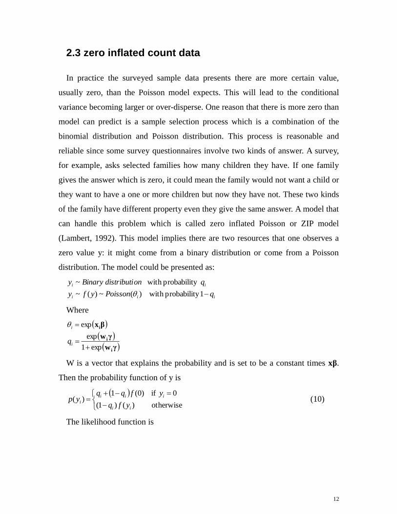
2.3 zero inflated count data
In practice the surveyed sample data presents there are more certain value,
usually zero, than the Poisson model expects. This will lead to the conditional
variance becoming larger or over-disperse. One reason that there is more zero than
model can predict is a sample selection process which is a combination of the
binomial distribution and Poisson distribution. This process is reasonable and
reliable since some survey questionnaires involve two kinds of answer. A survey,
for example, asks selected families how many children they have. If one family
gives the answer which is zero, it could mean the family would not want a child or
they want to have a one or more children but now they have not. These two kinds
of the family have different property even they give the same answer. A model that
can handle this problem which is called zero inflated Poisson or ZIP model
(Lambert, 1992). This model implies there are two resources that one observes a
zero value y: it might come from a binary distribution or come from a Poisson
distribution. The model could be presented as:
iii
ii
qPoissonyfy
qondistributiBinaryy
1y probabilit with )(~)(~
y probabilit with ~
Where
γw
γw
βx
i
i
i
exp1
exp
exp
i
i
q
W is a vector that explains the probability and is set to be a constant times xβ.
Then the probability function of y is
otherwise )()1(
0 if )0(1)(
ii
iii
iyfq
yfqqyp (10)
The likelihood function is
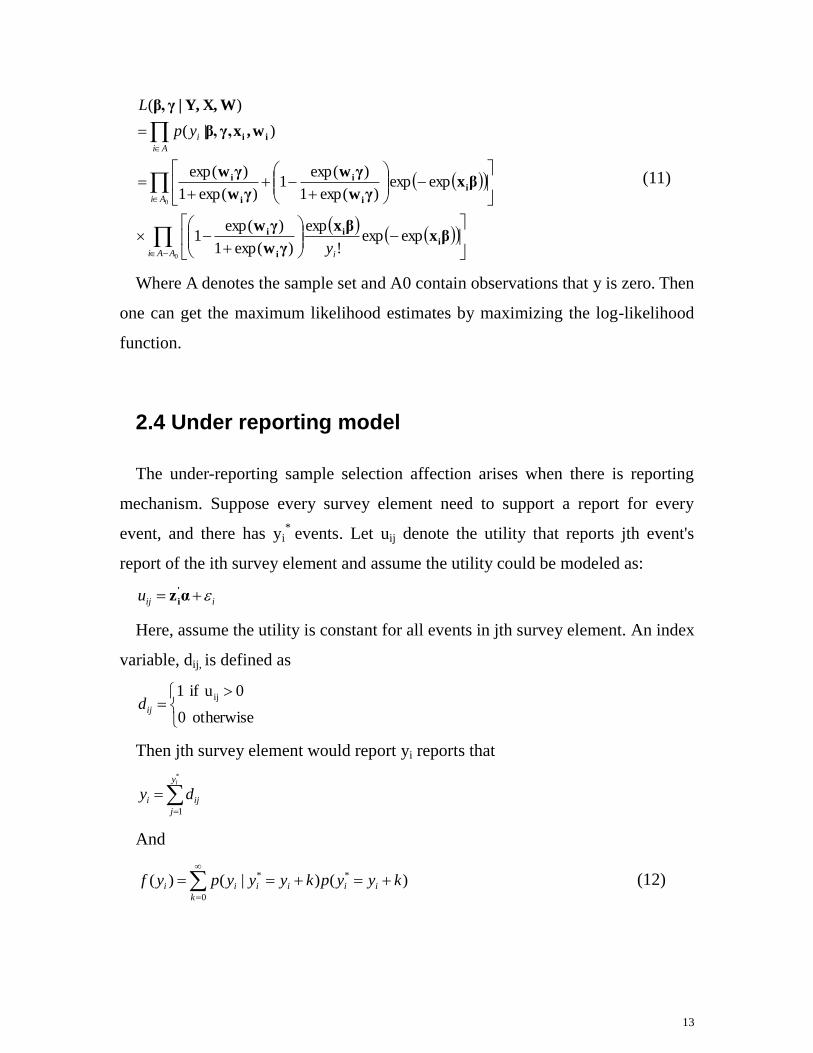
13
0
0
expexp!
exp
)exp(1
)exp(1
expexp)exp(1
)exp(1
)exp(1
)exp(
)|(
)(
AAi i
Ai
Ai
i
y
yp
L
βxβx
γw
γw
βxγw
γw
γw
γw
w,xγ,β,
WX,Y,|γβ,
ii
i
i
i
i
i
i
i
ii
(11)
Where A denotes the sample set and A0 contain observations that y is zero. Then
one can get the maximum likelihood estimates by maximizing the log-likelihood
function.
2.4 Under reporting model
The under-reporting sample selection affection arises when there is reporting
mechanism. Suppose every survey element need to support a report for every
event, and there has yi*
events. Let uij denote the utility that reports jth event's
report of the ith survey element and assume the utility could be modeled as:
iiju αz'
i
Here, assume the utility is constant for all events in jth survey element. An index
variable, dij, is defined as
otherwise 0
0u if 1 ij
ijd
Then jth survey element would report yi reports that
*
1
iy
j
iji dy
And
)()|()( *
0
* kyypkyyypyf ii
k
iiii
(12)

14
Where the conditional distribution of y is distributed as a binomial distribution
that
))(Pr,(~)|( *αzi iiiii obkyBinomialkyyyP
Winkelmann and Zimmermann (1993) give the complete model by assuming
that p (yi*) is distributed as Poisson with mean equal to exp (xβ) and ɛ is
distributed as logistic distribution. Under these assumptions
iy
i
i
iiii
yzxyf
!
)exp(),|(
(13)
where
)exp(1
)exp(
γz
γzβx'
i
'
i
'
i
i
Further they provide the maximum likelihood estimates.
2.5 endogenous switching and sample selection
Terza (1998) proposes a model and three estimators that deal with both sample
selection and endogenous switching. The model is constructed with two parts: a
Poisson equation that describes how independent variables influence the discrete
dependent variable; a selection equation that describes whether or not one element
in population would be observed or this element is affected by a treatment. The
endogenous switching model is given as
)exp(!
)(
i
y
iy
ypi
)exp( i
'
ii βcαx (14)
15
0 if 0
0 if 1
21
21
ii
ii
iz
zc
1
),(~),(
2
Σ
Σ0
where
Binomialf
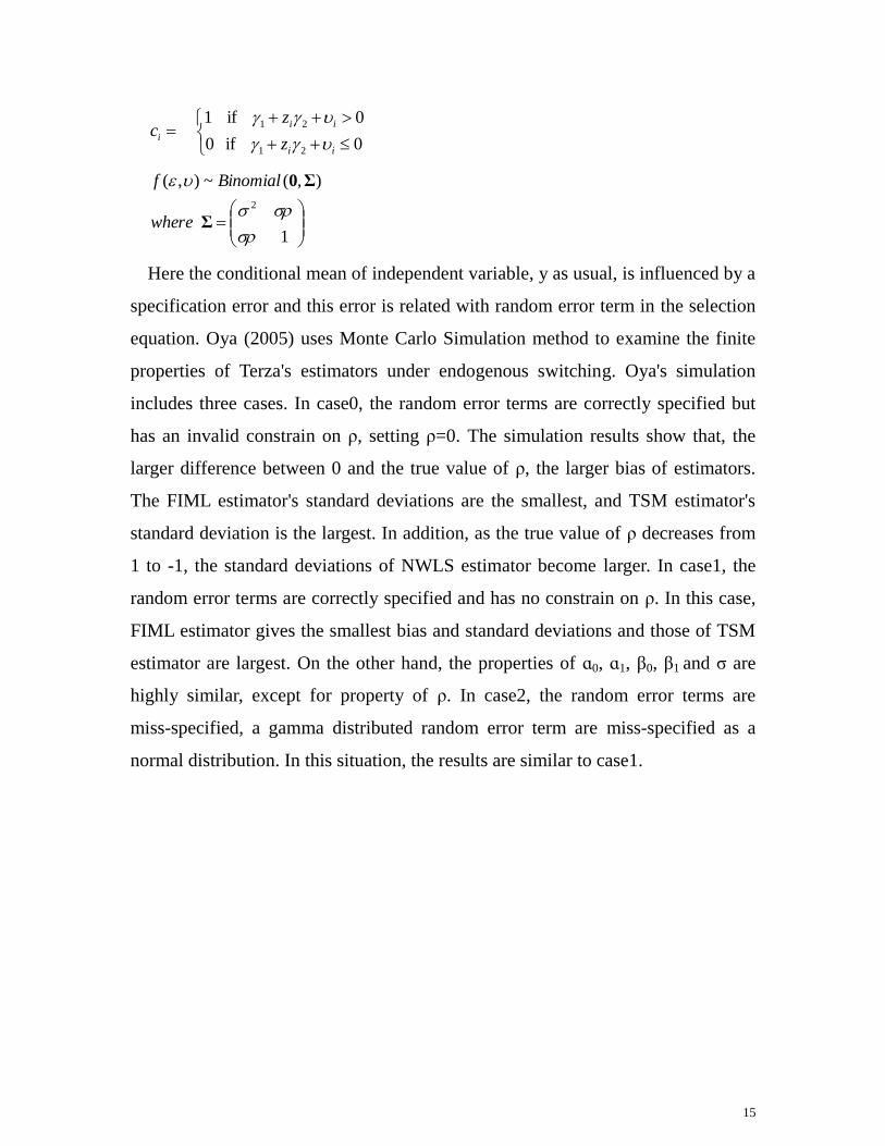
Here the conditional mean of independent variable, y as usual, is influenced by a
specification error and this error is related with random error term in the selection
equation. Oya (2005) uses Monte Carlo Simulation method to examine the finite
properties of Terza's estimators under endogenous switching. Oya's simulation
includes three cases. In case0, the random error terms are correctly specified but
has an invalid constrain on ρ, setting ρ=0. The simulation results show that, the
larger difference between 0 and the true value of ρ, the larger bias of estimators.
The FIML estimator's standard deviations are the smallest, and TSM estimator's
standard deviation is the largest. In addition, as the true value of ρ decreases from
1 to -1, the standard deviations of NWLS estimator become larger. In case1, the
random error terms are correctly specified and has no constrain on ρ. In this case,
FIML estimator gives the smallest bias and standard deviations and those of TSM
estimator are largest. On the other hand, the properties of ɑ0, ɑ1, β0, β1 and σ are
highly similar, except for property of ρ. In case2, the random error terms are
miss-specified, a gamma distributed random error term are miss-specified as a
normal distribution. In this situation, the results are similar to case1.
16
3. Estimators under the sample selection
effect
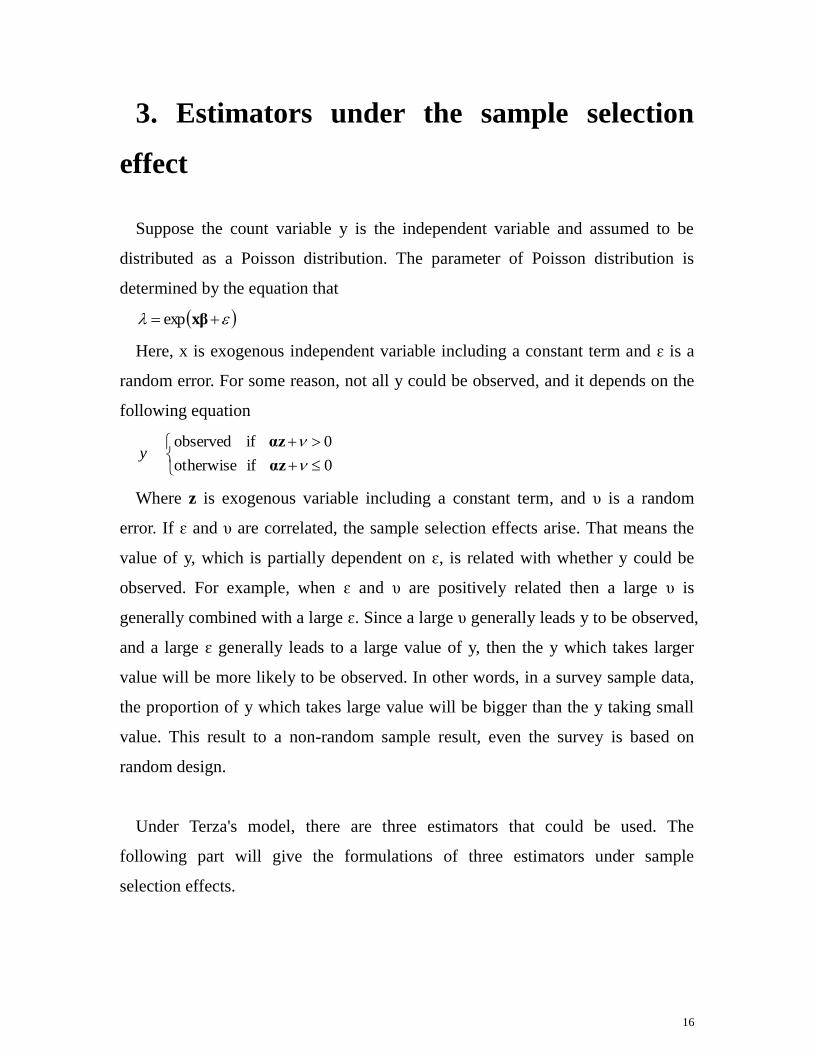
Suppose the count variable y is the independent variable and assumed to be
distributed as a Poisson distribution. The parameter of Poisson distribution is
determined by the equation that
xβexp
Here, x is exogenous independent variable including a constant term and ɛ is a
random error. For some reason, not all y could be observed, and it depends on the
following equation
0 if otherwise
0 if observed
αz
αzy
Where z is exogenous variable including a constant term, and υ is a random
error. If ɛ and υ are correlated, the sample selection effects arise. That means the
value of y, which is partially dependent on ɛ, is related with whether y could be
observed. For example, when ɛ and υ are positively related then a large υ is
generally combined with a large ɛ. Since a large υ generally leads y to be observed,
and a large ɛ generally leads to a large value of y, then the y which takes larger
value will be more likely to be observed. In other words, in a survey sample data,
the proportion of y which takes large value will be bigger than the y taking small
value. This result to a non-random sample result, even the survey is based on
random design.
Under Terza's model, there are three estimators that could be used. The
following part will give the formulations of three estimators under sample
selection effects.
17
3.1 FIML estimator
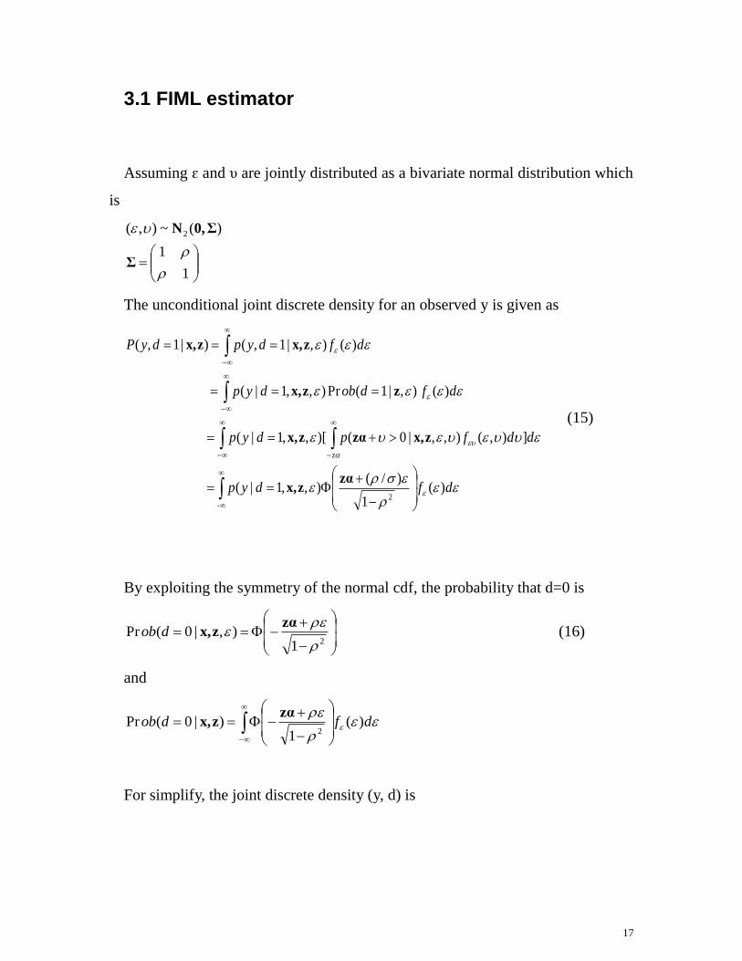
Assuming ɛ and υ are jointly distributed as a bivariate normal distribution which
is
1
1
)(~),( 2
Σ
Σ0,N
The unconditional joint discrete density for an observed y is given as
dfdyp
ddfpdyp
dfdobdyp
dfdypdyP
z
)(1
)/(),,1|(
]),(),,|0()[,,1|(
)( ),|1(Pr),,1|(
)(),|1,()|1,(
-2
zαzx,
zx,zαzx,
zzx,
zx,zx,
(15)
By exploiting the symmetry of the normal cdf, the probability that d=0 is
21),|0(Pr
zαzx,dob (16)
and
dfdob )(
1)|0(Pr
2
zαzx,
For simplify, the joint discrete density (y, d) is
18
d
d
ydd
dfd
ydPddyP
y
)exp(2
1
1
))/()(12(
))]exp(exp(!
)exp()1[(
)(1
))/()(12()],|()1[()|,(
2
2
2
2
zα
xβxβ
zαxzx,
(17)
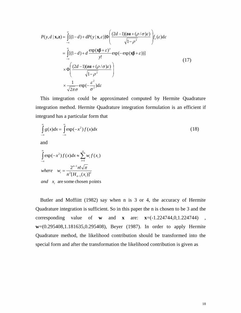
This integration could be approximated computed by Hermite Quadrature
integration method. Hermite Quadrature integration formulation is an efficient if
integrand has a particular form that
dxxfxdxxg )()exp()( 2 (18)
and
pointschosen some are
)]([
!2
)()()exp(
2
1
2
1
1
2
i
in
n
i
n
i
ii
xand
xHn
nwwhere
xfwdxxfx
Butler and Moffiitt (1982) say when n is 3 or 4, the accuracy of Hermite
Quadrature integration is sufficient. So in this paper the n is chosen to be 3 and the
corresponding value of w and x are: x=(-1.224744,0,1.224744) ,
w=(0.295408,1.181635,0.295408), Beyer (1987). In order to apply Hermite
Quadrature method, the likelihood contribution should be transformed into the
special form and after the transformation the likelihood contribution is given as
19
d
d
ydddyP
y
)exp(
1
)2)(12(
))]2exp(exp(!
)2exp()1[(
1 )|,(
2
2
zα
xβxβ
zx,
(19)
The conditional likelihood function is easily computed, and Fully Information
Maximum Likelihood estimators could be getting by maximizing the conditional
likelihood function.
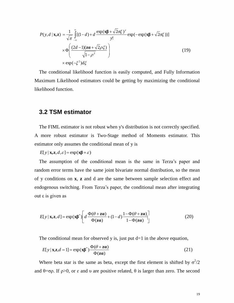
3.2 TSM estimator
The FIML estimator is not robust when y's distribution is not correctly specified.
A more robust estimator is Two-Stage method of Moments estimator. This
estimator only assumes the conditional mean of y is
)exp(],,|[ xβzx, dyE
The assumption of the conditional mean is the same in Terza’s paper and
random error terms have the same joint bivariate normal distribution, so the mean
of y conditions on x, z and d are the same between sample selection effect and
endogenous switching. From Terza’s paper, the conditional mean after integrating
out ε is given as
)(1
)(1)1(
)(
)()exp(],|[ *
zα
zα
zα
zαxβzx,
dddyE (20)
The conditional mean for observed y is, just put d=1 in the above equation,
)(
)()exp(]1|[ *
zα
zαxβzx
,d,yE (21)
Where beta star is the same as beta, except the first element is shifted by σ2/2
and θ=σρ. If ρ>0, or ɛ and υ are positive related, θ is larger than zero. The second

20
term on the right side of the above equation is larger than one. It could be seen as
an adjust term on the conditional mean of y because of the sample selection effects.
As mentioned above, a positive relation between ɛ and υ leads to increase the
proportion of larger value of y in observed data and increases the mean, as well.
The adjusted term makes the "inflated" mean of y closer to the original level, at
least. The expected difference between observed y and unobserved y is:
))(1)((
)()()exp(
))(1)((
)()()exp(
)(1
)(1
)(
)()exp(
]0,,|[]1,,|[
*
*
zαzα
zαzαxβ
zαzα
zαzαxβ
zα
zα
zα
zαxβ
zxzx
*
dyEdyE
(22)
For example, when the expectation of zα is 0.5 and σ is 0.3, the difference will
be increasing as ρ taking large absolutely value (table 1).
Table 1 The average percentage that the observed y is larger than unobserved y
ρ -0.8 -0.6 -0.4 -0.2 0 0.2 0.4 0.6 0.8
% -41 -30 -20 -10 0 9 19 28 36
given the expectation of zα is 0.5 and σ is 0.3
Now the estimated model could be written as

21
e
hy
)(
)()exp(
),,,,(
*
*
zα
zαxβ
βαzx
(23)
Where e is a random error term. This equation could be estimated by non-linear
least squares method or estimated by two-stage technique if beta and alpha have
larger dimensions. The first stage is a simple probit regression analysis and obtains
a consistent estimate of ɑ0 and ɑ1. The second-stage is a nonlinear least squares
method to
ehy ),,ˆ,,( * βαzx
Where are the estimates in the first stage. Denote vector b1= (β*, θ) and
Terza (1998) shows that the approximate distribution of b1 is given as
αg
bg
ggggαggggggD
D0bb
2
1
1
1
'
11
'
21
'
21
'
11
'
1
11
h
h
EEVAREeEE
where
Nnd
1'21 ][][)ˆ(][][][
],[)ˆ(
(24)
VAR ( α ) denotes the asymptotic covariance matrix of the first-stage probit
estimator of ɑ. In practice, a heteroskedasticity-consistent estimator of D could be
computed as
11 )]()ˆ(ˆ[)(ˆ 1
'
11
'
22
'
11
'
11
'
1 GGGGαGGΨGGGGD RAV
Where G1 and G2 are matrices whose typical rows are
αg
bg
2
1
1
ˆ
ˆˆ
ˆ
ˆˆ
h
h
and

22
nni
N
i
ediag
RAV
)}ˆ({
))ˆ(1)(ˆ(
)ˆ()ˆ(ˆ
2
1
1
2
Ψ
αzαz
zzαzα
'
i
'
i
i
'
i
'
i
3.3 NWLS method
Since the variance of a Poisson distribution is λ, so for different observations,
the conditional variance of y is mostly different. Then a weighted least-square
method could gain large efficient.
From Terza's paper, the conditional variance is given as
2
2
222 2exp
,,|),,|(),|(
zxzxzx yEVaryVarEeVar
Where
)exp(
)(/)(,
,22exp
*
2
2
xβ
zαzαα
α
(25)
Parameters ɑ, β* and θ can be obtained using two-stage estimators while σ
2
could be estimated by regression approach or conditional maximum likelihood
approach. Conditional maximum likelihood approach is reliable, but it is
computational cumbersome. Therefore, the regression based approach is used in
this paper. One can rearrange terms in var(e) in such way that
23
estimates stage- twoof value thetaking, are ˆˆˆˆ and
) (25 as defined
)exp(
)ˆ2exp(/ˆˆ
ˆˆˆˆˆ
2
2
22
2
2
2
ψψδeψψδe
ψψδe
ψδt
ψδψδer
tr
,,,,,,
,,,
a
where
a
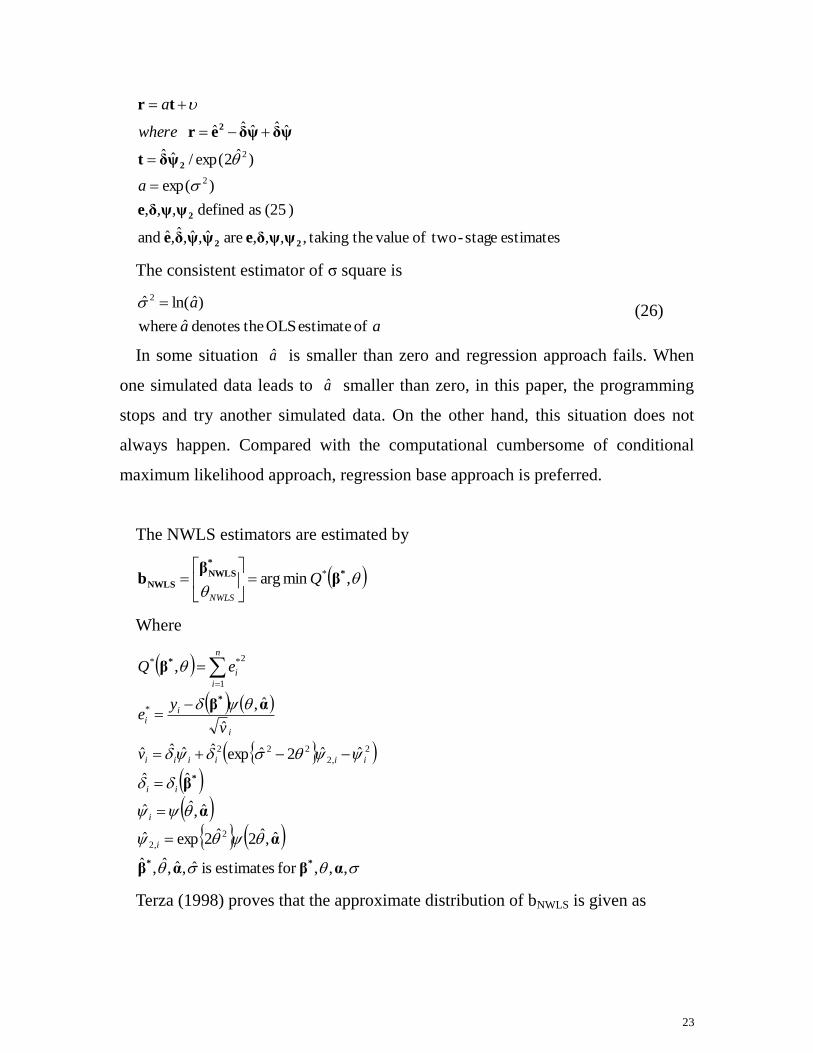
The consistent estimator of σ square is
aa
a
of estimate OLS thedenotes ˆ where
)ˆln(ˆ 2 (26)
In some situation a is smaller than zero and regression approach fails. When
one simulated data leads to a smaller than zero, in this paper, the programming
stops and try another simulated data. On the other hand, this situation does not
always happen. Compared with the computational cumbersome of conditional
maximum likelihood approach, regression base approach is preferred.
The NWLS estimators are estimated by
,minarg * *
*
NWLS
NWLS ββ
b QNWLS
Where
,,,for estimates is ˆ,ˆ,ˆ,ˆ
ˆ,ˆ2ˆ2expˆ
ˆ,ˆˆ
ˆˆ
ˆˆ2ˆexpˆˆˆˆ
ˆ
ˆ,
,
2
,2
2
,2
222
*
1
2**
αβαβ
α
α
β
αβ
β
**
*
*
*
i
i
ii
iiiiii
i
ii
n
i
i
v
v
ye
eQ
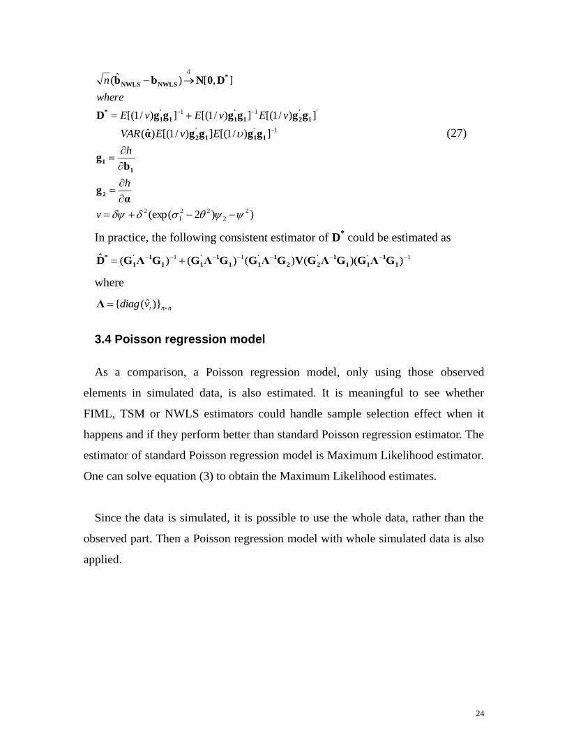
Terza (1998) proves that the approximate distribution of bNWLS is given as
24
))2(exp(
])/1[(])/1[()ˆ(
])/1[(])/1[(])/1[(
],[)ˆ(
2
2
22
1
2
1
'11
v
h
h
EvEVAR
vEvEvE
where
nd
αg
bg
ggggα
ggggggD
D0Nbb
2
1
1
1
'
11
'
2
1
'
21
'
11
'
1
*
*
NWLSNWLS
(27)
In practice, the following consistent estimator of D* could be estimated as
111 ))(()()()(ˆ 1
1'
11
1'
22
1'
11
1'
11
1'
1
*GΛGGΛGVGΛGGΛGGΛGD
where
nnivdiag )}ˆ({Λ
3.4 Poisson regression model
As a comparison, a Poisson regression model, only using those observed
elements in simulated data, is also estimated. It is meaningful to see whether
FIML, TSM or NWLS estimators could handle sample selection effect when it
happens and if they perform better than standard Poisson regression estimator. The
estimator of standard Poisson regression model is Maximum Likelihood estimator.
One can solve equation (3) to obtain the Maximum Likelihood estimates.
Since the data is simulated, it is possible to use the whole data, rather than the
observed part. Then a Poisson regression model with whole simulated data is also
applied.

25
4. Simulation design
The count-dependent variable yi, i=1, 2...500 are generated from the conditional
Poisson distribution, which is named as outcome equation:
ii
iiii
yxyf
exp
!
exp,|
and the conditional mean function is
iiii xx 22110exp
Not all of yi could be observed, and it is decided by the following selection
mechanism, which is named as selection equation:
0 if otherwise
0 if observed
22110
22110
iii
iii
izz
zzy
Where coefficient parameters in the model, (ɑ0, ɑ1, ɑ2, β0, β1, β2), are set different
values among simulation designs. The variance-covariance matrix of the error
terms ɛi and υi is set as
1
2
In the former papers , like Oya (2005), the simulation set up are different by
changing the value of ρ. There are, however, more potential factors that might be
impact on the performance of estimators. In this paper, simulation designs include
more variance, and examine four factors: the value of ρ, the value of σ, the
value of λ, and whether conditional mean equation has common variable with
selection equation.

26
The value of ρis the first factor that should be examine, and in theory the
estimates bias would not appears whenρis zero. So it should be expected in the
simulation results that, whenρis zero the estimates’ bias is not statistically
significant, or is the smallest one if other factors also cause estimates bias.
The second factor is the value of σ. The random error term presents the un-control
part of the regression model, so it also likely has influence on the performance of
estimators. On the other hand, the random error term in selection equation is not
changed, because the probit regression model has a constant variance of random
error term.
The third factor is the expected conditional mean,𝜆. As a characteristic of the
Poisson distribution, the mean of Poisson distribution is equal to the variance of
Poisson distribution, referred as equidisperson (Winkelmann, 2008, p8.). As
conditional mean increases, the conditional variance also becomes larger. This
might has an influence on estimators’ estimates. Another thing should be
mentioned, that the sample selection effect results a change on conditional mean of
the observed sub-sample of the whole population. Since the characteristic of
equidisperson, the conditional variance of sub-sample also different from the
conditional variance of the whole population. This maybe let a complicate
interactive impact between the value of 𝜌 and the value of 𝜆.
The last factor is whether or not the conditional mean equation has common
variable with the selection equation. This factor would more likely have an impact
on the TSM estimator and NWLS estimator. . In Terza's paper, "the TSM estimator
is a nonlinear least-squares analog to the popular Heckman estimator", and the
NWLS estimator is a weighted TSM estimator. So the TSM and the NWLS are
belonging to the Heckman's two-stage estimator. Puhani (2002) points out that
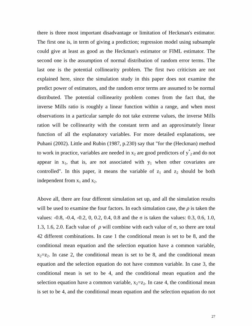
27
there is three most important disadvantage or limitation of Heckman's estimator.
The first one is, in term of giving a prediction; regression model using subsample
could give at least as good as the Heckman's estimator or FIML estimator. The
second one is the assumption of normal distribution of random error terms. The
last one is the potential collinearity problem. The first two criticism are not
explained here, since the simulation study in this paper does not examine the
predict power of estimators, and the random error terms are assumed to be normal
distributed. The potential collinearity problem comes from the fact that, the
inverse Mills ratio is roughly a linear function within a range, and when most
observations in a particular sample do not take extreme values, the inverse Mills
ration will be collinearity with the constant term and an approximately linear
function of all the explanatory variables. For more detailed explanations, see
Puhani (2002). Little and Rubin (1987, p.230) say that "for the (Heckman) method
to work in practice, variables are needed in x2 are good predictors of y*2 and do not
appear in x1, that is, are not associated with y1 when other covariates are
controlled". In this paper, it means the variable of z1 and z2 should be both
independent from x1 and x2.
Above all, there are four different simulation set up, and all the simulation results
will be used to examine the four factors. In each simulation case, the 𝜌 is taken the
values: -0.8, -0.4, -0.2, 0, 0.2, 0.4, 0.8 and the σ is taken the values: 0.3, 0.6, 1.0,
1.3, 1.6, 2.0. Each value of 𝜌 will combine with each value of σ, so there are total
42 different combinations. In case 1 the conditional mean is set to be 8, and the
conditional mean equation and the selection equation have a common variable,
x2=z2. In case 2, the conditional mean is set to be 8, and the conditional mean
equation and the selection equation do not have common variable. In case 3, the
conditional mean is set to be 4, and the conditional mean equation and the
selection equation have a common variable, x2=z2. In case 4, the conditional mean
is set to be 4, and the conditional mean equation and the selection equation do not

28
have a common variable.
The explanatory variable x1, x2 are generated from a uniform distribution over the
interval between 0 and 2. z2 is also generated from a uniform distribution over the
interval between 0 and 2. z1 is set to be equal to x1 or is generated from a uniform
distribution. In this paper, each simulation experiment is conducted by 1000 times.
One detail should be mentioned, that in order to test whether the σ will influence
the performance of estimator, the σ takes different values. However, changing σ's
value will change the expectation of conditional mean or E(λi). This could be
shown by the following equation:
)2
1exp()exp(
)][exp()exp(
)][exp(][
2
xβ
xβ
xβ
E
EE
(28)
In order to control a same conditional mean for different σ's value, β0 is
adjusted that the conditional mean is unchanged. The rest coefficient parameters
are set to be (ɑ0, ɑ1, ɑ2, β1, β2) = (0.2, 0.2, 0.4, 0.6, 0.4) when 𝜆 is 8, and (ɑ0, ɑ1,
ɑ2, β1, β2) = (0.2, 0.2, 0.4, 0.3, 0.2) when 𝜆 is 4. Table 2 is a summary of
simulation set up for each simulation case.

29
Table 2, the summary of simulation set up
Case 1 Case 2 Case 3 Case 4
𝜆 8 8 4 4
x1 U (0,2) U (0,2) U (0,2) U (0,2)
x2 U (0,2) U (0,2) U (0,2) U (0,2)
z1 U (0,2) U (0,2) U (0,2) U (0,2)
z2 =x1 U (0,2) =x1 U (0,2)
(ɑ0, ɑ1, ɑ2) (0.2, 0.2, 0.4) (0.2, 0.2, 0.4) (0.2, 0.2, 0.4) (0.2, 0.2, 0.4)
(β1, β2) (0.6, 0.4) (0.6, 0.4) (0.3, 0.2) (0.3, 0.2)
β0
𝜎=0.3 1.034442 1.034442 0.3412944 0.3412944
𝜎=0.6 0.8994415 0.8994415 0.2062944 0.2062944
𝜎=1.0 0.5794415 0.5794415 -0.1137056 -0.1137056
𝜎=1.3 0.2344415 0.2344415 -0.4587056 -0.4587056
𝜎=1.6 -0.2005585 -0.2005585 -0.8937056 -0.8937056
𝜎=2.0 -0.9205585 -0.9205585 -1.613706 -1.613706
30
5. Simulation results
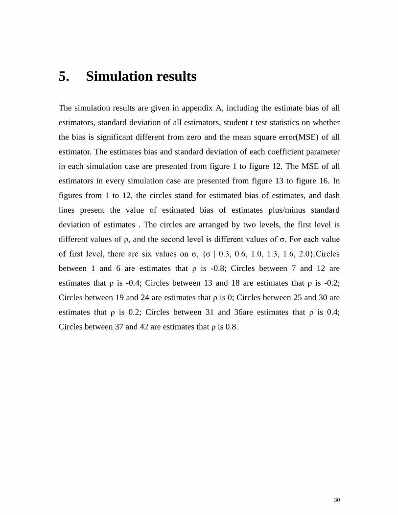
The simulation results are given in appendix A, including the estimate bias of all
estimators, standard deviation of all estimators, student t test statistics on whether
the bias is significant different from zero and the mean square error(MSE) of all
estimator. The estimates bias and standard deviation of each coefficient parameter
in each simulation case are presented from figure 1 to figure 12. The MSE of all
estimators in every simulation case are presented from figure 13 to figure 16. In
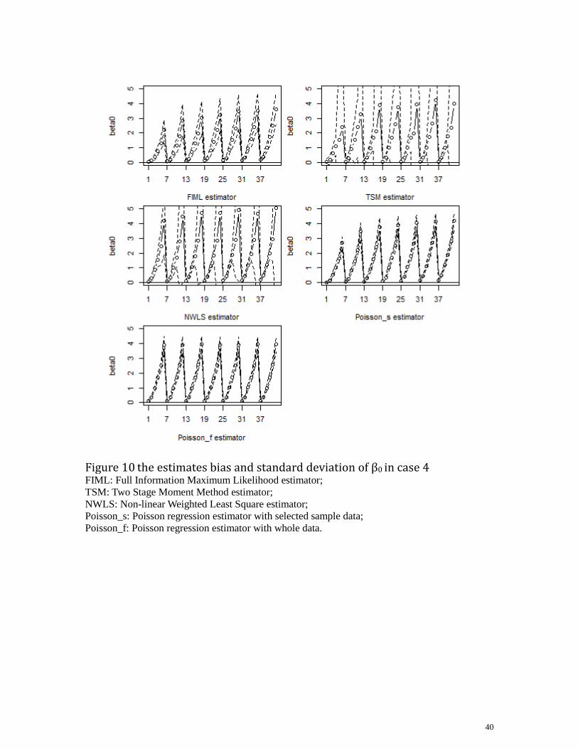
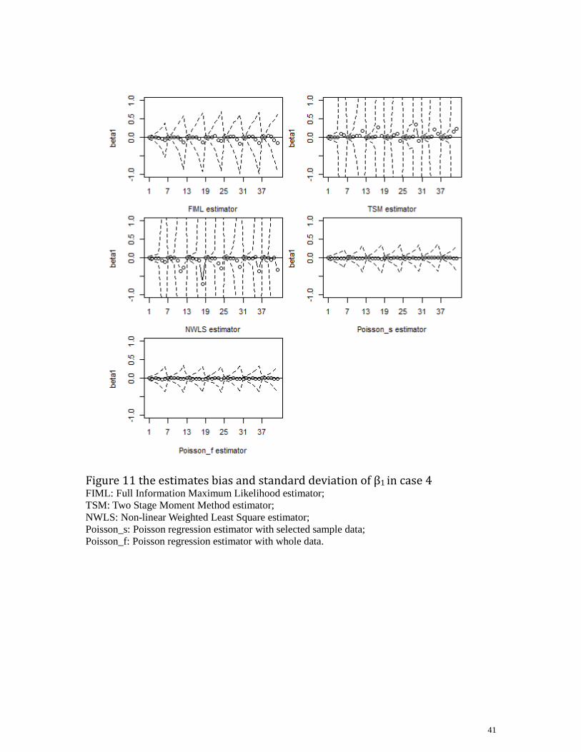
figures from 1 to 12, the circles stand for estimated bias of estimates, and dash
lines present the value of estimated bias of estimates plus/minus standard
deviation of estimates . The circles are arranged by two levels, the first level is
different values of ρ, and the second level is different values of σ. For each value
of first level, there are six values on σ, {σ | 0.3, 0.6, 1.0, 1.3, 1.6, 2.0}.Circles
between 1 and 6 are estimates that ρ is -0.8; Circles between 7 and 12 are
estimates that ρ is -0.4; Circles between 13 and 18 are estimates that ρ is -0.2;
Circles between 19 and 24 are estimates that ρ is 0; Circles between 25 and 30 are
estimates that ρ is 0.2; Circles between 31 and 36are estimates that ρ is 0.4;
Circles between 37 and 42 are estimates that ρ is 0.8.
31
Figure 1 the estimates bias and standard deviation of β0 in case 1 FIML: Full Information Maximum Likelihood estimator;
TSM: Two Stage Moment Method estimator;
NWLS: Non-linear Weighted Least Square estimator;
Poisson_s: Poisson regression estimator with selected sample data;
Poisson_f: Poisson regression estimator with whole data.

32
Figure 2, the estimates bias and standard deviation of β1 in case 1 FIML: Full Information Maximum Likelihood estimator;
TSM: Two Stage Moment Method estimator;
NWLS: Non-linear Weighted Least Square estimator;
Poisson_s: Poisson regression estimator with selected sample data;
Poisson_f: Poisson regression estimator with whole data.
33
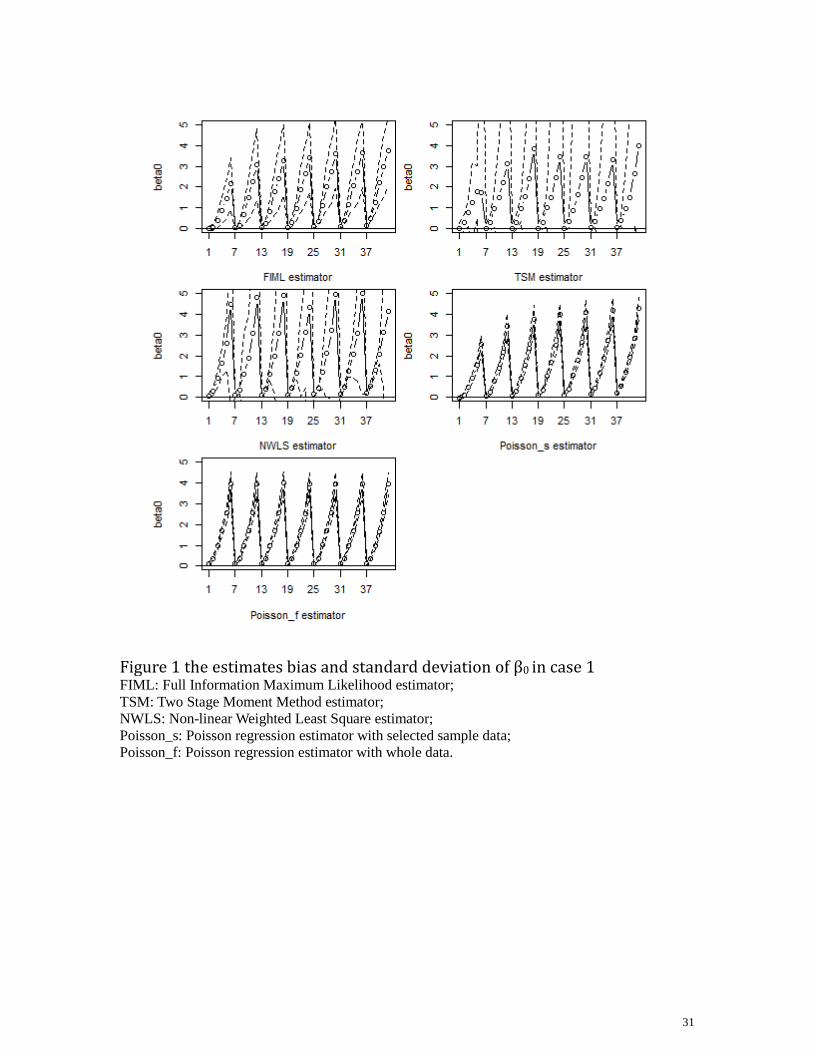
Figure 3 the estimates bias and standard deviation of β2 in case 1 FIML: Full Information Maximum Likelihood estimator;
TSM: Two Stage Moment Method estimator;
NWLS: Non-linear Weighted Least Square estimator;
Poisson_s: Poisson regression estimator with selected sample data;
Poisson_f: Poisson regression estimator with whole data.

34
Figure 4 the estimates bias and standard deviation of β0 in case 2 FIML: Full Information Maximum Likelihood estimator;
TSM: Two Stage Moment Method estimator;
NWLS: Non-linear Weighted Least Square estimator;
Poisson_s: Poisson regression estimator with selected sample data;
Poisson_f: Poisson regression estimator with whole data.

35
Figure 5 the estimates bias and standard deviation of β1 in case 2 FIML: Full Information Maximum Likelihood estimator;
TSM: Two Stage Moment Method estimator;
NWLS: Non-linear Weighted Least Square estimator;
Poisson_s: Poisson regression estimator with selected sample data;
Poisson_f: Poisson regression estimator with whole data.

36
Figure 6 the estimates bias and standard deviation of β2 in case 2 FIML: Full Information Maximum Likelihood estimator;
TSM: Two Stage Moment Method estimator;
NWLS: Non-linear Weighted Least Square estimator;
Poisson_s: Poisson regression estimator with selected sample data;
Poisson_f: Poisson regression estimator with whole data.

37
Figure 7 the estimates bias and standard deviation of β0 in case 3 FIML: Full Information Maximum Likelihood estimator;
TSM: Two Stage Moment Method estimator;
NWLS: Non-linear Weighted Least Square estimator;
Poisson_s: Poisson regression estimator with selected sample data;
Poisson_f: Poisson regression estimator with whole data.

38
Figure 8 the estimates bias and standard deviation of β1 in case 3 FIML: Full Information Maximum Likelihood estimator;
TSM: Two Stage Moment Method estimator;
NWLS: Non-linear Weighted Least Square estimator;
Poisson_s: Poisson regression estimator with selected sample data;
Poisson_f: Poisson regression estimator with whole data.
39
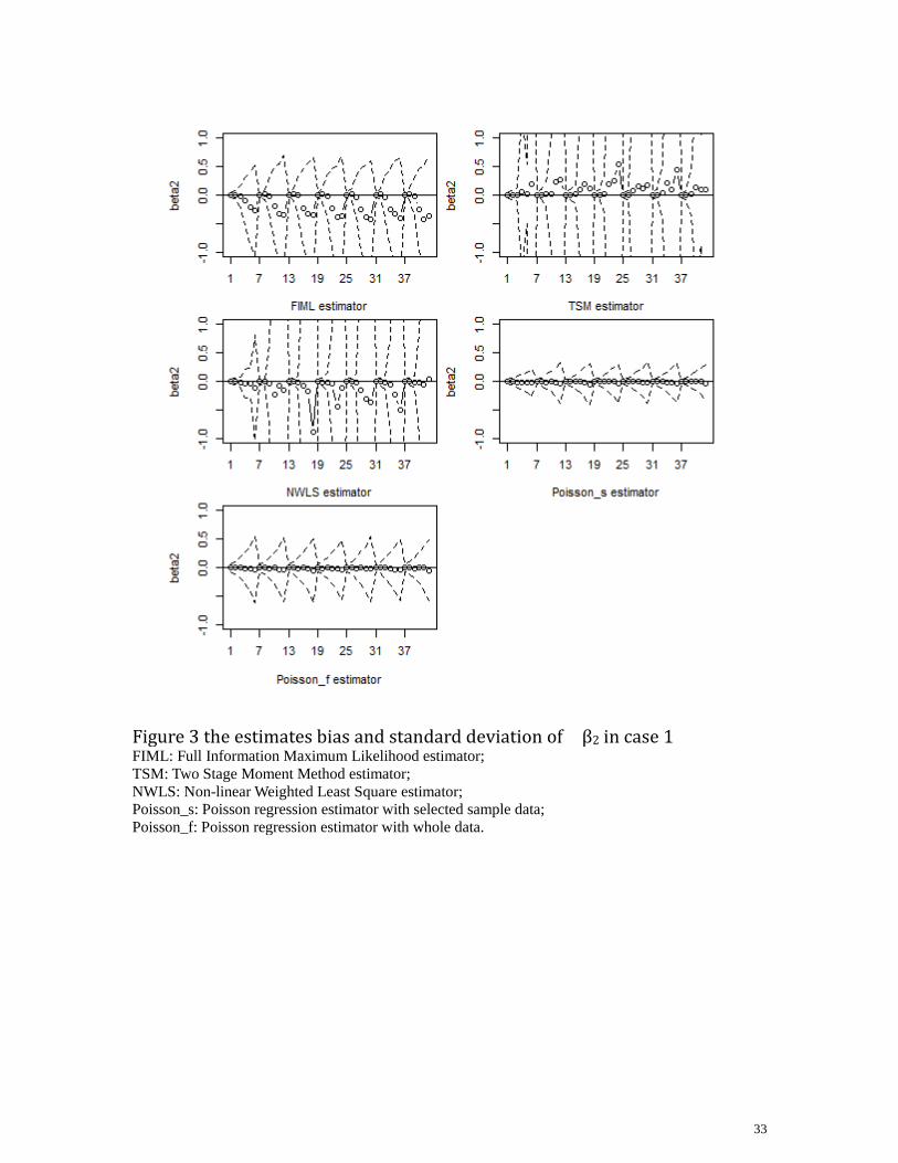
Figure 9 the estimates bias and standard deviation of β2 in case 3 FIML: Full Information Maximum Likelihood estimator;
TSM: Two Stage Moment Method estimator;
NWLS: Non-linear Weighted Least Square estimator;
Poisson_s: Poisson regression estimator with selected sample data;
Poisson_f: Poisson regression estimator with whole data.
40
Figure 10 the estimates bias and standard deviation of β0 in case 4 FIML: Full Information Maximum Likelihood estimator;
TSM: Two Stage Moment Method estimator;
NWLS: Non-linear Weighted Least Square estimator;
Poisson_s: Poisson regression estimator with selected sample data;
Poisson_f: Poisson regression estimator with whole data.
41
Figure 11 the estimates bias and standard deviation of β1 in case 4 FIML: Full Information Maximum Likelihood estimator;
TSM: Two Stage Moment Method estimator;
NWLS: Non-linear Weighted Least Square estimator;
Poisson_s: Poisson regression estimator with selected sample data;
Poisson_f: Poisson regression estimator with whole data.

42
Figure 12 the estimates bias and standard deviation of β2 in case 4 FIML: Full Information Maximum Likelihood estimator;
TSM: Two Stage Moment Method estimator;
NWLS: Non-linear Weighted Least Square estimator;
Poisson_s: Poisson regression estimator with selected sample data;
Poisson_f: Poisson regression estimator with whole data.

43
Figure 13 Relative MSE, TSM estimator as the benchmark, in case 1 The line with circle presents the relative MSE of FIML estimator
The line without circle presents the relative MSE of NWLS estimator
44
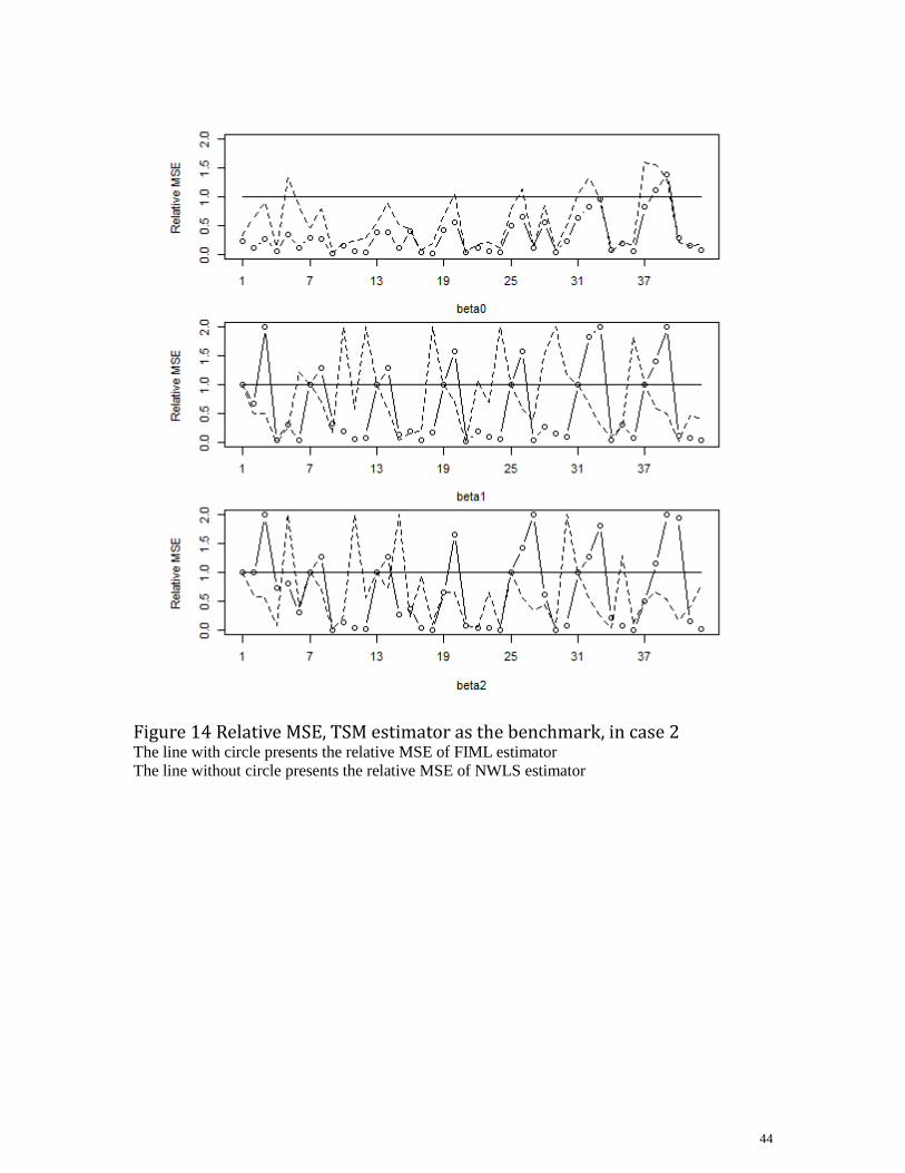
Figure 14 Relative MSE, TSM estimator as the benchmark, in case 2 The line with circle presents the relative MSE of FIML estimator
The line without circle presents the relative MSE of NWLS estimator

45
Figure 15 Relative MSE, TSM estimator as the benchmark, in case 3 The line with circle presents the relative MSE of FIML estimator
The line without circle presents the relative MSE of NWLS estimator
46
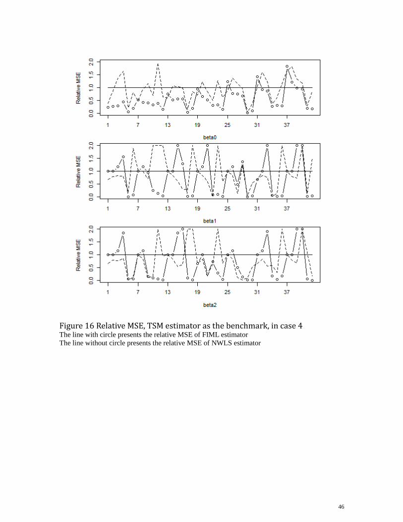
Figure 16 Relative MSE, TSM estimator as the benchmark, in case 4 The line with circle presents the relative MSE of FIML estimator
The line without circle presents the relative MSE of NWLS estimator

47
6. Comments on simulation results
6.1 The bias of estimates
6.1.1 The impact of 𝝈 and 𝝆 on estimate bias
The four estimators, even Poisson_f estimator, result significant estimate bias on
constant independent variable (β0), meanwhile, the estimate bias is increasing as σ
taking larger value. Among them, FIML estimator has the smallest bias and NWLS
estimator has the largest in most causes. Except FIML estimator, the estimate bias
of rest estimators are all cause by misidentify on constant independent variable
(β0). As mentioned in Terza’s paper (Terza 1998), the estimated β0 by TSM
estimator or NWLS estimator is actually the value of β0 sifted by σ2/2. The
estimate bias when applying Poisson_s or Poisson_f estimator is cause by
unobserved heterogeneity. Rainer Winkelmann says (Winkelmann 2008, p128), if
one assumes the unobserved heterogeneity has the following characteristics:
𝐸[exp(ε) |𝑥] = 𝐸[exp (𝜀)]
the mean conditional on x, but unconditional on 𝜀 is
𝐸[𝑦|𝑥] = exp(𝛼 + 𝑥′𝛽) 𝐸[exp(𝜀) |𝑥] = exp (�� + 𝑥′𝛽)
where �� = 𝛼 + 𝑙𝑜𝑔𝐸[exp (𝜀)]. The value of 𝐸[exp (𝜀)] is increase as σ becomes
larger. As a comparison, FIML estimator control the unobserved heterogeneity by
integrating out the 𝜀 in Likelihood function, the estimate bias of β0 is less than the
estimate bias of Poisson_f estimator or Poisson_s estimator.
β1 is the coefficient of independent variable, which is appears in both conditional

48
mean equation and selection equation. Poisson_f estimator performs quite well,
and it indicates that the unobserved heterogeneity does not cause series harm, at
least not cause significant bias. Just as Rainer Winkelmann says (Winkelmann
2008, p129), the Pseudo-Maximum Likelihood estimator can provide “consistent
parameter estimates and valid inference based on Poisson model.” FIML, TSM,
NWLS and Poisson_s estimators, that using selected sample data, result biased
estimates on β1 in most cases.
There is a quite clear pattern, which is shared by FIML, TSM and NWLS
estimators, that the bias of estimates quickly increases while 𝜎 becomes larger.
Among these three estimators, the increasing scale of estimates bias is more
serious on FIML estimator and on NWLS estimator. On the other hand, the value
of 𝜌 has less influence on the bias of estimates. Another characteristic is FIML
and NWLS estimators’ under-estimate the parameter in most cases, while TSM
estimator over-estimates the parameter.
The Poisson_s estimator performances quite well, smaller bias and lower standard
deviation. The parameter 𝜌 has a clear impact on Poisson_s estimator, that when
𝜌 takes negative value, the estimate bias of Poisson_s estimator is positive and
when 𝜌 takes positive value, the estimate bias of Poisson_s estimator is negative.
What’s more, the larger 𝜌 in absolutely value, the estimate bias becomes large,
also in absolutely value. On the other hand, the value of 𝜎 has little influence on
the estimates of Poisson_s estimator, which is quite different from FIML, TSM
and NWLS estimators.
β2 is the coefficient of independent variable that only appears in conditional mean
equation. The estimates of β2 of all estimators are better than the estimates of β1,
and each estimator have the similar performance as they do on β1.
49
6.1.2 The impact of the common variable on estimate bias
Comparing case1 with case 2 , or case 3 with case 4, whether or not the
conditional mean equation has common variable with the selection equation has
influence on the performance of all estimators. Generally speaking, if there are no
common variables between two equations, the bias of estimates of all estimators
would be smaller than that if there has common variables, and the improvement of
bias on coefficient parameter β1 is more significant than that on coefficient
parameter β2.
6.1.3 The impact of 𝝀 on estimate bias
Comparing case 1, case 2 with case 3, case 4, a smaller expected conditional mean
would give a lower estimate bias on all estimators. The reason might also be the
equidisperson characteristic of Poisson distribution. The smaller mean of Poisson
distribution means a lower variance at the same time.
6.2 The Mean Square Error (MSE)
The above all discussion focus on the estimate bias (the accuracy of an estimator),
but the variance of an estimator (the precision of an estimator) should be also
considered. So it is meaning full to examine the mean squared error (MSE) as well.
A smaller MSE indicates the estimator could have a smaller combined variance
and bias. Figure 13 to figure 16 display the relative MSE of FIML, NWLS and
TSM estimators, which TSM’s MSE as the benchmark. The MSE of Poisson_s
estimator is not shown on these figures, because it is almost lower than any of
50
FIML, TSM and NWLS estimators’ (for detail, see Appendix A).
6.2.1 The impact of 𝝈 and 𝝆 on MSE
As the impact on estimate bias, the value of 𝜌 alos has a smaller influence on
MSE compared with the value of 𝜎. The impact of 𝜎 on MSE, however, is more
complicated than the effect on estimate bias. When 𝜎 is lower, such as 0.3 or 0.6
in this paper, the MSE of FIML and NWLS are lower (or equal) than TSM’s, when
𝜎 becomes larger, such as 1.0 or 1.3 in this paper, the MSE of FIML and NWLS
are over the TSM’s, but if 𝜎 still increases, such as 1.6 or 2.0, the MSE of FIML
and NWLS are lower again than TSM’s. This means the impact of σ on MSE of
estimators is not a constant trend, or not monotonously.
6.2.2 The impact of common variable
The MSE of coefficient parameter 𝛽2 is not significant influenced by whether or
not there has common variable between the conditional mean equation and the
selection equation. On the other hand, the MSE of coefficient parameter 𝛽1 is
influenced by this factor. If there is common variable, the MSE of FIML and
NWLS estimators are lower than TSM’s when 𝜎 is small, such as 0.3 , and if
there is no common variable, the MSE of FIML and NWLS estimators are roughly
equal to the TSM’s when 𝜎 is small, such as 0.3 .
6.2.3 The impact of 𝝀
The scale of the conditional mean might not have significant influence on the
relative MSE of all estimators.
51
7. The conclusion
Sample selection effects are common in Econometrics analysis, labor market,
Health Economics and so on. FIML estimator and TSM estimator or NWLS
estimator are two kinds of usually used estimators to hand the sample selection
effects. In this paper, a simulation study is performed and these estimators’
properties are examined. Base on the simulation results, there are some
conclusions, which could be used to choose the better one among these estimators:
1. Whether or not the conditional mean equation and selection equation have
common variables have a significant impact on estimates. Generally speaking,
less common variables in both conditional mean equation and selection
equation, the better performance of all estimators is.
2. When conditional mean equation and selection equation have common
variables, the TSM estimator always overestimates the coefficients of the
common variables, the FIML and NWLS estimator always underestimates the
coefficients of the common variables, the Poisson_s estimator overestimates
the coefficients of the common variables when correlation between two
random error terms is close to -1 and underestimates when correlation is close
to 1.
3. When conditional mean equation and selection equation have common
variables, the estimate bias of FIML estimator, TSM estimator and NWLS
estimator is all un-robust on the variance of random error term in conditional
equation.
52
4. When conditional mean equation and selection equation have common
variables, the MSE of NWLS estimator is lower than TSM estimator’s if the
variance of random error term in conditional equation is small. As the variance
of random error term increasing, the MSE of FIML and NWLS become larger
than TSM’s, but they become smaller again than TSM’s if the variance of
random error term still increases. Meanwhile, the MSE of Poisson_s estimator
always lowers than TSM’s and NWLS’s.
5. There is not simple rule to choose the best estimator among FIML, TSM and
NWLS estimators. None of them is always give the lowest estimate bias and
lowest MSE in all simulation cases.
6. Even Poisson_s estimator does not handle the sample selection effect, it is
more robust and simple to use. Poisson_s estimator is more preferred;
especially the random error term in conditional mean is thought to be large.

53
Reference
Beyer, W.H. (1987). CRC Standard Mathematical Tables. 28th ed. Boca Raton, FL: CRC
Press. 464.
Butler, J S and Moffitt, R. (1982). A Computationally Efficient Quadrature Procedure for
the One-Factor Multinomial Probit Model.Econometrica. 50 (3), 761-764.
Felix, F and Wang, W. (2004). Censored generalized Poisson regression model.
Computational Statistics & Data Analysis. 46 (3), 547-560.
Greene, W.H (1994). Sample Selection in the Poisson Regression Model, Department of
Economics, Stern School of Business, New York University.
Grogger, J. T and Carson, R. T. (1991). Models for Truncated Counts.Journal of Applied
Econometrics. 6 (3), 225-238.
Gronau, G. (1974). Wage Comparisons--A Selectivity Bias. Journal of Political Economy.
82 (6), 1119-1143.
Heckman, J. (1974). Shadow Prices, Market Wages, and Labor Supply. Econometrica. 42
(4), 679-694.
Lambert, D. (1992). Zero-Inflated Poisson Regression, with an Application to Defects in
Manufacturing. Technometrics. 34 (1), 1-14.
Lee, L F. (1983). Generalized Econometric Models with Selectivity.Econometrica. 51 (2),
507-512.
Little, R. J. A. and Rubin, D. B. (1987). Statistical Analysis with Missing Data. New
York: John Wiley & Sons. p230.
Oya, K. (2005). Properties of estimators of count data model with endogenous switching.
Mathematics and Computers in Simulation. 68 (5-6), 536-544.
Puhani. P. (2002). The Heckman Correction for Sample Selection and Its

54
Critique. You have free access to this content Journal of Economic Surveys. 14 (1),
p53-68.
Romeu, A and Vera-Hernández, M. (2005). Counts with an endogenous binary
regressor: A series expansion approach. The Econometrics Journal. 8 (1), 1-22.
Terza, J V. (1998). Estimating count data models with endogenous switching: Sample
selection and endogenous treatment effects. Journal of Econometrics. 84 (1), 129-154.
Vella , F. (1998). Estimating Models with Sample Selection Bias: A Survey. The Journal of
Human Resources. 33 (1), 127-169.
William, G. (2009). Models for count data with endogenous participation. Empirical
Economics. 36 (1), 133-173.
Winkelmann, R (2008). Econometric Analysis Of Count Data. 5th ed. Berlin: Springer.
p8, p128-129.

55
Appendix A
The following tables list simulation results in this paper.
56
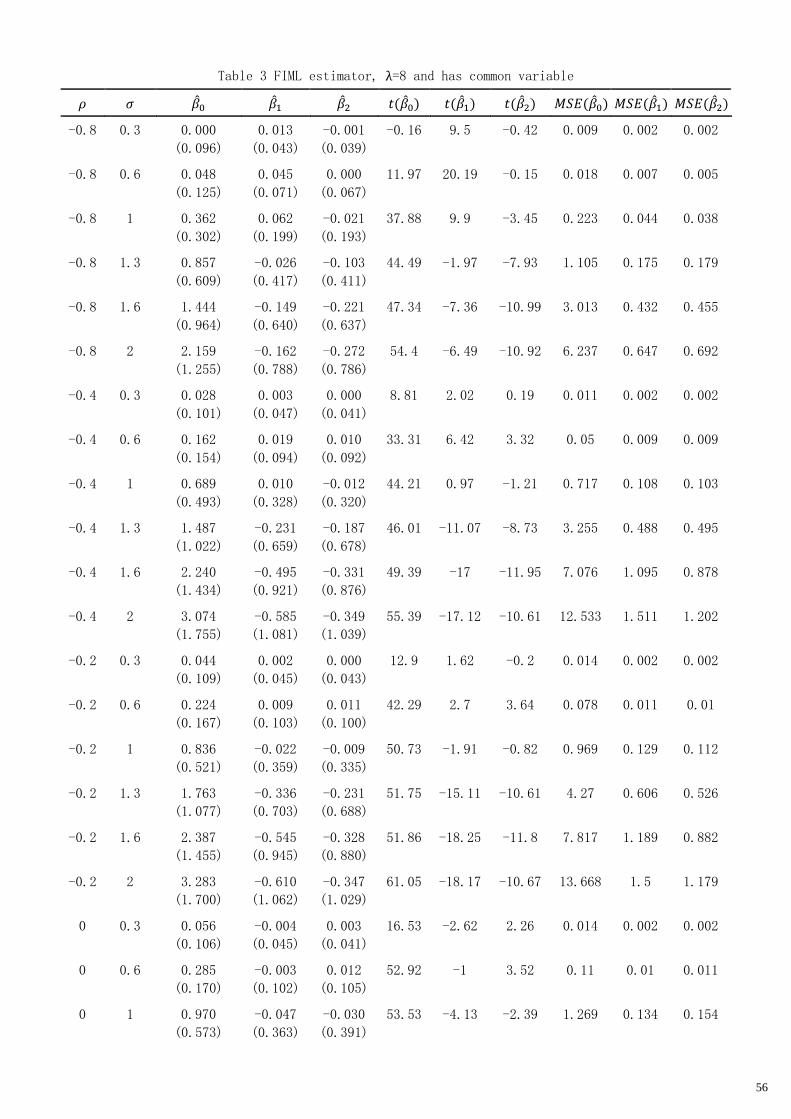
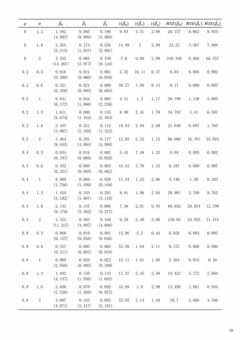
Table 3 FIML estimator, λ=8 and has common variable
𝜌 𝜎 ��0 ��1 ��2 𝑡(��0) 𝑡(��1) 𝑡(��2) 𝑀𝑆𝐸(��0) 𝑀𝑆𝐸(��1) 𝑀𝑆𝐸(��2)
-0.8 0.3 0.000
(0.096)
0.013
(0.043)
-0.001
(0.039)
-0.16 9.5 -0.42 0.009 0.002 0.002
-0.8 0.6 0.048
(0.125)
0.045
(0.071)
0.000
(0.067)
11.97 20.19 -0.15 0.018 0.007 0.005
-0.8 1 0.362
(0.302)
0.062
(0.199)
-0.021
(0.193)
37.88 9.9 -3.45 0.223 0.044 0.038
-0.8 1.3 0.857
(0.609)
-0.026
(0.417)
-0.103
(0.411)
44.49 -1.97 -7.93 1.105 0.175 0.179
-0.8 1.6 1.444
(0.964)
-0.149
(0.640)
-0.221
(0.637)
47.34 -7.36 -10.99 3.013 0.432 0.455
-0.8 2 2.159
(1.255)
-0.162
(0.788)
-0.272
(0.786)
54.4 -6.49 -10.92 6.237 0.647 0.692
-0.4 0.3 0.028
(0.101)
0.003
(0.047)
0.000
(0.041)
8.81 2.02 0.19 0.011 0.002 0.002
-0.4 0.6 0.162
(0.154)
0.019
(0.094)
0.010
(0.092)
33.31 6.42 3.32 0.05 0.009 0.009
-0.4 1 0.689
(0.493)
0.010
(0.328)
-0.012
(0.320)
44.21 0.97 -1.21 0.717 0.108 0.103
-0.4 1.3 1.487
(1.022)
-0.231
(0.659)
-0.187
(0.678)
46.01 -11.07 -8.73 3.255 0.488 0.495
-0.4 1.6 2.240
(1.434)
-0.495
(0.921)
-0.331
(0.876)
49.39 -17 -11.95 7.076 1.095 0.878
-0.4 2 3.074
(1.755)
-0.585
(1.081)
-0.349
(1.039)
55.39 -17.12 -10.61 12.533 1.511 1.202
-0.2 0.3 0.044
(0.109)
0.002
(0.045)
0.000
(0.043)
12.9 1.62 -0.2 0.014 0.002 0.002
-0.2 0.6 0.224
(0.167)
0.009
(0.103)
0.011
(0.100)
42.29 2.7 3.64 0.078 0.011 0.01
-0.2 1 0.836
(0.521)
-0.022
(0.359)
-0.009
(0.335)
50.73 -1.91 -0.82 0.969 0.129 0.112
-0.2 1.3 1.763
(1.077)
-0.336
(0.703)
-0.231
(0.688)
51.75 -15.11 -10.61 4.27 0.606 0.526
-0.2 1.6 2.387
(1.455)
-0.545
(0.945)
-0.328
(0.880)
51.86 -18.25 -11.8 7.817 1.189 0.882
-0.2 2 3.283
(1.700)
-0.610
(1.062)
-0.347
(1.029)
61.05 -18.17 -10.67 13.668 1.5 1.179
0 0.3 0.056
(0.106)
-0.004
(0.045)
0.003
(0.041)
16.53 -2.62 2.26 0.014 0.002 0.002
0 0.6 0.285
(0.170)
-0.003
(0.102)
0.012
(0.105)
52.92 -1 3.52 0.11 0.01 0.011
0 1 0.970
(0.573)
-0.047
(0.363)
-0.030
(0.391)
53.53 -4.13 -2.39 1.269 0.134 0.154

57
𝜌 𝜎 ��0 ��1 ��2 𝑡(��0) 𝑡(��1) 𝑡(��2) 𝑀𝑆𝐸(��0) 𝑀𝑆𝐸(��1) 𝑀𝑆𝐸(��2)
0 1.3 1.882
(1.113)
-0.351
(0.727)
-0.240
(0.701)
53.48 -15.28 -10.82 4.782 0.652 0.549
0 1.6 2.622
(1.447)
-0.601
(0.967)
-0.394
(0.907)
57.31 -19.67 -13.75 8.971 1.297 0.978
0 2 3.401
(1.697)
-0.662
(1.090)
-0.370
(1.035)
63.37 -19.2 -11.31 14.447 1.627 1.208
0.2 0.3 0.080
(0.106)
-0.006
(0.043)
0.000
(0.043)
23.83 -4.06 0.02 0.018 0.002 0.002
0.2 0.6 0.319
(0.165)
0.000
(0.103)
0.009
(0.102)
61.32 0.13 2.88 0.129 0.011 0.01
0.2 1 1.101
(0.571)
-0.092
(0.383)
-0.039
(0.356)
60.95 -7.63 -3.47 1.538 0.155 0.128
0.2 1.3 2.017
(1.129)
-0.399
(0.727)
-0.248
(0.717)
56.51 -17.35 -10.93 5.344 0.688 0.575
0.2 1.6 2.728
(1.527)
-0.619
(0.963)
-0.383
(0.921)
56.51 -20.31 -13.15 9.774 1.31 0.996
0.2 2 3.603
(1.675)
-0.684
(1.089)
-0.427
(1.016)
68.01 -19.85 -13.27 15.787 1.654 1.215
0.4 0.3 0.098
(0.105)
-0.012
(0.045)
0.002
(0.043)
29.53 -8.42 1.78 0.021 0.002 0.002
0.4 0.6 0.374
(0.163)
-0.015
(0.100)
0.014
(0.100)
72.66 -4.64 4.45 0.166 0.01 0.01
0.4 1 1.136
(0.567)
-0.083
(0.368)
-0.033
(0.378)
63.37 -7.14 -2.76 1.613 0.142 0.144
0.4 1.3 2.061
(1.121)
-0.393
(0.712)
-0.245
(0.694)
58.15 -17.44 -11.17 5.502 0.661 0.541
0.4 1.6 2.755
(1.539)
-0.659
(0.987)
-0.320
(0.907)
56.62 -21.14 -11.17 9.961 1.408 0.924
0.4 2 3.638
(1.691)
-0.667
(1.095)
-0.404
(1.033)
68.04 -19.26 -12.36 16.092 1.642 1.229
0.8 0.3 0.120
(0.105)
-0.015
(0.042)
0.001
(0.039)
36.27 -11.33 0.52 0.025 0.002 0.002
0.8 0.6 0.459
(0.149)
-0.034
(0.088)
0.012
(0.089)
97.29 -12.2 4.35 0.233 0.009 0.008
0.8 1 1.227
(0.509)
-0.098
(0.341)
-0.022
(0.324)
76.24 -9.14 -2.16 1.765 0.126 0.106
0.8 1.3 2.201
(1.070)
-0.437
(0.706)
-0.253
(0.711)
65.05 -19.55 -11.26 5.989 0.689 0.57
0.8 1.6 2.974
(1.507)
-0.699
(0.927)
-0.423
(0.951)
62.43 -23.85 -14.06 11.116 1.349 1.084
0.8 2 3.743
(1.657)
-0.720
(1.066)
-0.359
(1.040)
71.44 -21.37 -10.92 16.755 1.655 1.209

58
Table 4 TSM estimator, 𝜆=8 and has common variable
𝜌 𝜎 ��0 ��1 ��2 𝑡(��0) 𝑡(��1) 𝑡(��2) 𝑀𝑆𝐸(��0) 𝑀𝑆𝐸(��1) 𝑀𝑆𝐸(��2)
-0.8 0.3 -0.023
(0.259)
0.029
(0.077)
-0.001
(0.046)
-2.79 11.88 -0.42 0.067 0.007 0.002
-0.8 0.6 0.264
(0.384)
0.031
(0.108)
0.003
(0.073)
21.74 9.03 1.28 0.217 0.013 0.005
-0.8 1 0.752
(0.677)
0.062
(0.171)
0.003
(0.129)
35.12 11.5 0.85 1.024 0.033 0.017
-0.8 1.3 1.236
(1.945)
0.107
(0.445)
0.053
(1.364)
20.09 7.62 1.23 5.312 0.209 1.864
-0.8 1.6 1.762
(1.275)
0.172
(0.430)
0.021
(0.525)
43.72 12.61 1.27 4.729 0.215 0.276
-0.8 2 1.743
(16.939)
0.539
(4.504)
0.187
(5.653)
3.25 3.78 1.05 289.961 20.58 31.994
-0.4 0.3 -0.023
(0.243)
0.029
(0.077)
0.000
(0.048)
-2.96 11.83 -0.2 0.059 0.007 0.002
-0.4 0.6 0.265
(0.344)
0.026
(0.109)
0.003
(0.083)
24.31 7.49 1.11 0.188 0.012 0.007
-0.4 1 0.939
(0.897)
0.045
(0.305)
0.009
(0.210)
33.1 4.7 1.33 1.687 0.095 0.044
-0.4 1.3 1.491
(2.855)
0.180
(2.471)
0.015
(1.008)
16.51 2.31 0.46 10.373 6.136 1.017
-0.4 1.6 2.222
(5.579)
0.238
(2.448)
0.229
(2.769)
12.59 3.08 2.62 36.063 6.051 7.72
-0.4 2 3.140
(10.214)
0.432
(3.968)
0.267
(4.974)
9.72 3.44 1.7 114.18 15.932 24.811
-0.2 0.3 -0.013
(0.230)
0.029
(0.073)
0.000
(0.050)
-1.74 12.5 -0.05 0.053 0.006 0.002
-0.2 0.6 0.286
(0.320)
0.024
(0.106)
0.002
(0.088)
28.2 7.29 0.87 0.184 0.012 0.008
-0.2 1 0.977
(0.653)
0.032
(0.203)
0.009
(0.166)
47.33 5 1.75 1.38 0.042 0.028
-0.2 1.3 1.554
(2.740)
0.104
(1.075)
0.099
(1.248)
17.93 3.05 2.52 9.92 1.167 1.567
-0.2 1.6 2.406
(5.051)
0.204
(2.354)
0.191
(2.668)
15.06 2.73 2.27 31.304 5.585 7.152
-0.2 2 3.858
(6.234)
0.149
(1.880)
0.118
(3.345)
19.57 2.51 1.11 53.747 3.557 11.2
0 0.3 0.000
(0.211)
0.025
(0.069)
0.003
(0.048)
0.06 11.41 1.8 0.045 0.005 0.002
0 0.6 0.306
(0.298)
0.019
(0.099)
0.000
(0.087)
32.53 6.04 0.12 0.182 0.01 0.008
0 1 1.016
(0.922)
0.022
(0.286)
0.023
(0.330)
34.81 2.44 2.21 1.882 0.082 0.11
59
𝜌 𝜎 ��0 ��1 ��2 𝑡(��0) 𝑡(��1) 𝑡(��2) 𝑀𝑆𝐸(��0) 𝑀𝑆𝐸(��1) 𝑀𝑆𝐸(��2)
0 1.3 1.492
(4.892)
0.085
(0.809)
0.196
(2.986)
9.64 3.31 2.08 26.157 0.662 8.954
0 1.6 2.455
(5.215)
0.173
(1.827)
0.256
(2.801)
14.89 3 2.89 33.22 3.367 7.909
0 2 3.455
(14.367)
0.084
(2.977)
0.539
(8.134)
7.6 0.89 2.09 218.348 8.868 66.457
0.2 0.3 0.016
(0.200)
0.021
(0.066)
0.001
(0.048)
2.52 10.11 0.47 0.04 0.005 0.002
0.2 0.6 0.321
(0.259)
0.021
(0.095)
0.000
(0.083)
39.27 7.05 0.13 0.17 0.009 0.007
0.2 1 0.841
(6.172)
0.044
(1.066)
0.083
(2.236)
4.31 1.3 1.17 38.799 1.138 5.005
0.2 1.3 1.611
(5.674)
0.090
(1.184)
0.145
(2.563)
8.98 2.41 1.78 34.792 1.41 6.591
0.2 1.6 2.437
(3.887)
0.221
(2.459)
0.112
(1.323)
19.83 2.84 2.69 21.048 6.097 1.763
0.2 2 3.464
(8.655)
0.291
(4.084)
0.177
(4.999)
12.65 2.25 1.12 86.906 16.761 25.024
0.4 0.3 0.034
(0.197)
0.016
(0.068)
0.002
(0.050)
5.43 7.49 1.32 0.04 0.005 0.003
0.4 0.6 0.352
(0.251)
0.008
(0.094)
0.003
(0.082)
44.33 2.78 1.23 0.187 0.009 0.007
0.4 1 0.980
(1.786)
0.069
(1.409)
0.029
(0.449)
17.34 1.55 2.06 4.149 1.99 0.203
0.4 1.3 1.459
(5.182)
0.103
(1.667)
0.201
(3.118)
8.91 1.96 2.04 28.981 2.789 9.762
0.4 1.6 2.145
(9.179)
0.347
(5.462)
0.086
(3.577)
7.39 2.01 0.76 88.852 29.954 12.799
0.4 2 3.322
(11.315)
0.383
(4.887)
0.448
(4.606)
9.28 2.48 3.08 139.05 24.025 21.415
0.8 0.3 0.060
(0.157)
0.010
(0.058)
0.001
(0.046)
12.06 5.2 0.44 0.028 0.004 0.002
0.8 0.6 0.357
(0.211)
0.005
(0.087)
0.005
(0.076)
53.58 1.64 2.11 0.172 0.008 0.006
0.8 1 0.980
(2.050)
0.029
(0.902)
0.023
(0.399)
15.11 1.01 1.86 5.164 0.815 0.16
0.8 1.3 1.492
(4.147)
0.150
(1.936)
0.133
(1.693)
11.37 2.45 2.49 19.425 3.772 2.884
0.8 1.6 2.656
(2.538)
0.078
(1.369)
0.092
(0.972)
33.09 1.8 2.98 13.495 1.881 0.954
0.8 2 3.997
(4.871)
0.163
(2.417)
0.095
(2.181)
25.95 2.14 1.38 39.7 5.868 4.766

60
Table 5 NWLS estimator, 𝜆=8 and has common variable
𝜌 𝜎 ��0 ��1 ��2 𝑡(��0) 𝑡(��1) 𝑡(��2) 𝑀𝑆𝐸(��0) 𝑀𝑆𝐸(��1) 𝑀𝑆𝐸(��2)
-0.8 0.3 0.067
(0.128)
-0.005
(0.051)
-0.002
(0.040)
16.65 -3.27 -1.41 0.021 0.003 0.002
-0.8 0.6 0.298
(0.209)
-0.005
(0.076)
-0.005
(0.060)
45.07 -2.08 -2.48 0.133 0.006 0.004
-0.8 1 0.939
(0.439)
-0.023
(0.126)
-0.012
(0.094)
67.68 -5.88 -4.11 1.073 0.016 0.009
-0.8 1.3 1.643
(0.688)
-0.027
(0.263)
-0.031
(0.248)
75.52 -3.24 -3.91 3.171 0.07 0.062
-0.8 1.6 2.584
(1.281)
-0.078
(0.416)
-0.033
(0.257)
63.79 -5.93 -4 8.32 0.179 0.067
-0.8 2 4.484
(5.145)
-0.234
(3.148)
-0.104
(0.923)
27.56 -2.35 -3.56 46.572 9.965 0.864
-0.4 0.3 0.093
(0.109)
-0.008
(0.050)
-0.002
(0.041)
26.76 -5.41 -1.41 0.021 0.003 0.002
-0.4 0.6 0.360
(0.188)
-0.014
(0.077)
-0.003
(0.066)
60.58 -5.69 -1.4 0.165 0.006 0.004
-0.4 1 1.105
(2.010)
-0.036
(0.189)
-0.039
(0.646)
17.38 -6.01 -1.9 5.259 0.037 0.419
-0.4 1.3 1.894
(2.147)
-0.075
(0.656)
-0.226
(4.615)
27.9 -3.6 -1.55 8.198 0.436 21.349
-0.4 1.6 3.079
(3.935)
-0.326
(5.336)
-0.069
(1.303)
24.74 -1.93 -1.68 24.962 28.577 1.703
-0.4 2 4.795
(5.908)
-0.682
(4.851)
-0.156
(4.912)
25.67 -4.45 -1.01 57.898 23.995 24.151
-0.2 0.3 0.109
(0.107)
-0.009
(0.047)
-0.003
(0.042)
32.43 -6.16 -1.91 0.023 0.002 0.002
-0.2 0.6 0.387
(0.151)
-0.017
(0.074)
-0.005
(0.067)
81.19 -7.32 -2.21 0.173 0.006 0.004
-0.2 1 1.099
(0.333)
-0.047
(0.134)
-0.015
(0.121)
104.46 -11.05 -3.84 1.319 0.02 0.015
-0.2 1.3 1.978
(1.848)
-0.188
(1.515)
-0.082
(2.239)
33.84 -3.92 -1.15 7.326 2.33 5.022
-0.2 1.6 3.078
(5.517)
-0.426
(4.836)
-0.177
(5.098)
17.64 -2.79 -1.1 39.906 23.569 26.017
-0.2 2 4.890
(8.176)
-0.720
(8.426)
-0.889
(13.579)
18.91 -2.7 -2.07 90.766 71.512 185.186
0 0.3 0.122
(0.089)
-0.013
(0.045)
0.001
(0.040)
43.29 -8.85 0.68 0.023 0.002 0.002
0 0.6 0.435
(0.192)
-0.023
(0.075)
-0.008
(0.069)
71.68 -9.85 -3.79 0.226 0.006 0.005
0 1 1.157
(0.339)
-0.054
(0.179)
-0.014
(0.165)
107.78 -9.62 -2.73 1.453 0.035 0.028

61
𝜌 𝜎 ��0 ��1 ��2 𝑡(��0) 𝑡(��1) 𝑡(��2) 𝑀𝑆𝐸(��0) 𝑀𝑆𝐸(��1) 𝑀𝑆𝐸(��2)
0 1.3 2.011
(1.990)
-0.119
(0.624)
-0.038
(1.002)
31.95 -6.04 -1.21 8.002 0.404 1.006
0 1.6 3.149
(2.688)
-0.592
(6.118)
-0.449
(5.000)
37.04 -3.06 -2.84 17.142 37.775 25.197
0 2 4.323
(8.982)
-0.302
(4.811)
-0.119
(7.642)
15.22 -1.99 -0.49 99.366 23.236 58.412
0.2 0.3 0.142
(0.086)
-0.014
(0.043)
-0.001
(0.042)
52.57 -10.38 -1.13 0.028 0.002 0.002
0.2 0.6 0.452
(0.134)
-0.021
(0.071)
-0.005
(0.064)
106.38 -9.47 -2.67 0.222 0.005 0.004
0.2 1 1.228
(0.863)
-0.053
(0.370)
-0.013
(0.159)
45.03 -4.53 -2.57 2.253 0.139 0.025
0.2 1.3 2.115
(2.190)
-0.182
(1.837)
-0.147
(2.698)
30.54 -3.13 -1.72 9.27 3.409 7.303
0.2 1.6 3.216
(3.226)
-0.326
(2.779)
-0.306
(6.312)
31.52 -3.7 -1.53 20.745 7.831 39.937
0.2 2 4.977
(5.793)
-0.587
(4.129)
-0.367
(5.595)
27.17 -4.49 -2.08 58.325 17.393 31.441
0.4 0.3 0.159
(0.081)
-0.019
(0.044)
0.000
(0.042)
62.02 -13.67 0.27 0.032 0.002 0.002
0.4 0.6 0.492
(0.130)
-0.033
(0.068)
-0.004
(0.064)
120.17 -15.64 -2 0.259 0.006 0.004
0.4 1 1.240
(0.279)
-0.070
(0.146)
-0.015
(0.115)
140.48 -15.23 -4.14 1.616 0.026 0.013
0.4 1.3 2.095
(1.199)
-0.177
(1.340)
-0.057
(0.823)
55.26 -4.17 -2.19 5.826 1.827 0.681
0.4 1.6 3.099
(2.302)
-0.154
(1.675)
-0.226
(3.694)
42.58 -2.91 -1.94 14.902 2.831 13.7
0.4 2 5.016
(4.888)
-0.594
(12.691)
-0.505
(6.529)
32.45 -1.48 -2.45 49.05 161.408 42.885
0.8 0.3 0.196
(0.071)
-0.024
(0.040)
-0.001
(0.039)
87.78 -19.38 -0.76 0.043 0.002 0.001
0.8 0.6 0.540
(0.107)
-0.043
(0.060)
-0.001
(0.059)
160.08 -22.73 -0.6 0.303 0.006 0.004
0.8 1 1.289
(0.291)
-0.076
(0.181)
-0.009
(0.111)
140.03 -13.23 -2.54 1.746 0.038 0.012
0.8 1.3 2.063
(0.472)
-0.169
(1.666)
-0.013
(0.864)
138.24 -3.2 -0.46 4.48 2.804 0.747
0.8 1.6 3.127
(2.641)
-0.332
(3.424)
-0.046
(2.214)
37.44 -3.06 -0.66 16.753 11.831 4.902
0.8 2 4.165
(17.023)
-0.355
(3.468)
0.043
(8.408)
7.74 -3.24 0.16 307.129 12.153 70.697
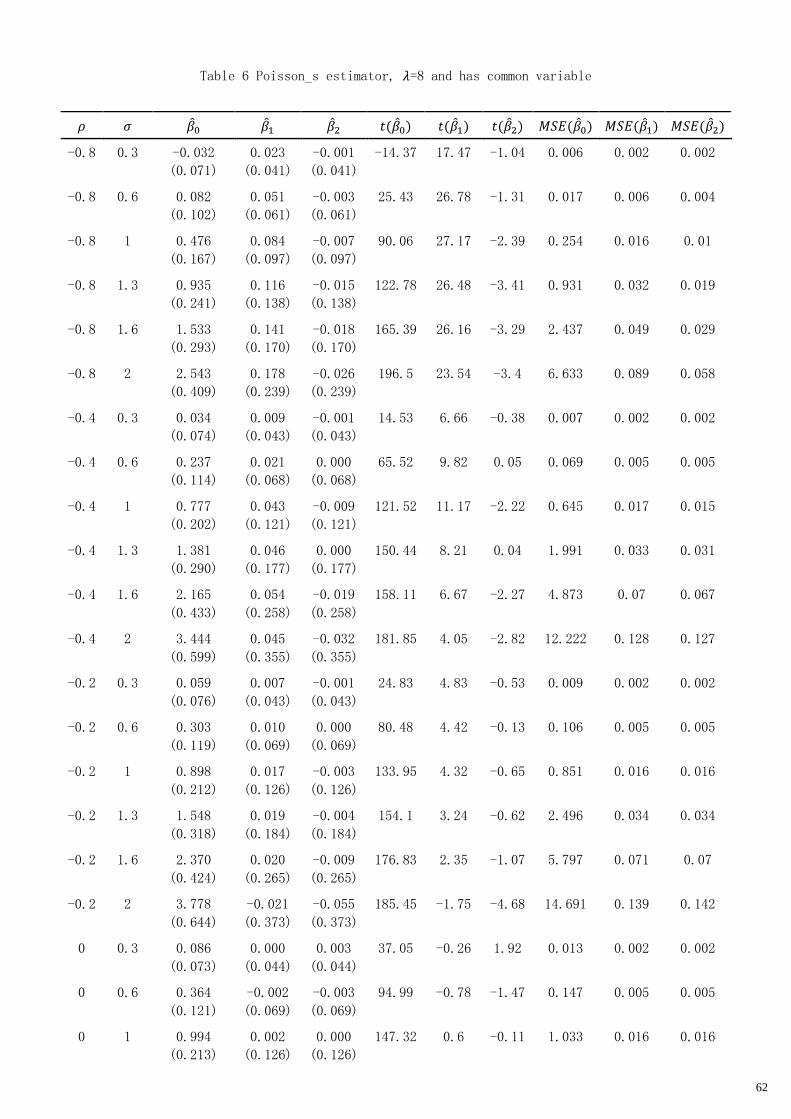
62
Table 6 Poisson_s estimator, 𝜆=8 and has common variable
𝜌 𝜎 ��0 ��1 ��2 𝑡(��0) 𝑡(��1) 𝑡(��2) 𝑀𝑆𝐸(��0) 𝑀𝑆𝐸(��1) 𝑀𝑆𝐸(��2)
-0.8 0.3 -0.032
(0.071)
0.023
(0.041)
-0.001
(0.041)
-14.37 17.47 -1.04 0.006 0.002 0.002
-0.8 0.6 0.082
(0.102)
0.051
(0.061)
-0.003
(0.061)
25.43 26.78 -1.31 0.017 0.006 0.004
-0.8 1 0.476
(0.167)
0.084
(0.097)
-0.007
(0.097)
90.06 27.17 -2.39 0.254 0.016 0.01
-0.8 1.3 0.935
(0.241)
0.116
(0.138)
-0.015
(0.138)
122.78 26.48 -3.41 0.931 0.032 0.019
-0.8 1.6 1.533
(0.293)
0.141
(0.170)
-0.018
(0.170)
165.39 26.16 -3.29 2.437 0.049 0.029
-0.8 2 2.543
(0.409)
0.178
(0.239)
-0.026
(0.239)
196.5 23.54 -3.4 6.633 0.089 0.058
-0.4 0.3 0.034
(0.074)
0.009
(0.043)
-0.001
(0.043)
14.53 6.66 -0.38 0.007 0.002 0.002
-0.4 0.6 0.237
(0.114)
0.021
(0.068)
0.000
(0.068)
65.52 9.82 0.05 0.069 0.005 0.005
-0.4 1 0.777
(0.202)
0.043
(0.121)
-0.009
(0.121)
121.52 11.17 -2.22 0.645 0.017 0.015
-0.4 1.3 1.381
(0.290)
0.046
(0.177)
0.000
(0.177)
150.44 8.21 0.04 1.991 0.033 0.031
-0.4 1.6 2.165
(0.433)
0.054
(0.258)
-0.019
(0.258)
158.11 6.67 -2.27 4.873 0.07 0.067
-0.4 2 3.444
(0.599)
0.045
(0.355)
-0.032
(0.355)
181.85 4.05 -2.82 12.222 0.128 0.127
-0.2 0.3 0.059
(0.076)
0.007
(0.043)
-0.001
(0.043)
24.83 4.83 -0.53 0.009 0.002 0.002
-0.2 0.6 0.303
(0.119)
0.010
(0.069)
0.000
(0.069)
80.48 4.42 -0.13 0.106 0.005 0.005
-0.2 1 0.898
(0.212)
0.017
(0.126)
-0.003
(0.126)
133.95 4.32 -0.65 0.851 0.016 0.016
-0.2 1.3 1.548
(0.318)
0.019
(0.184)
-0.004
(0.184)
154.1 3.24 -0.62 2.496 0.034 0.034
-0.2 1.6 2.370
(0.424)
0.020
(0.265)
-0.009
(0.265)
176.83 2.35 -1.07 5.797 0.071 0.07
-0.2 2 3.778
(0.644)
-0.021
(0.373)
-0.055
(0.373)
185.45 -1.75 -4.68 14.691 0.139 0.142
0 0.3 0.086
(0.073)
0.000
(0.044)
0.003
(0.044)
37.05 -0.26 1.92 0.013 0.002 0.002
0 0.6 0.364
(0.121)
-0.002
(0.069)
-0.003
(0.069)
94.99 -0.78 -1.47 0.147 0.005 0.005
0 1 0.994
(0.213)
0.002
(0.126)
0.000
(0.126)
147.32 0.6 -0.11 1.033 0.016 0.016

63
𝜌 𝜎 ��0 ��1 ��2 𝑡(��0) 𝑡(��1) 𝑡(��2) 𝑀𝑆𝐸(��0) 𝑀𝑆𝐸(��1) 𝑀𝑆𝐸(��2)
0 1.3 1.682
(0.325)
0.000
(0.188)
-0.005
(0.188)
163.54 0.05 -0.83 2.936 0.035 0.035
0 1.6 2.524
(0.441)
-0.016
(0.256)
-0.002
(0.256)
180.92 -1.92 -0.24 6.565 0.066 0.065
0 2 3.976
(0.575)
-0.059
(0.342)
-0.044
(0.342)
218.48 -5.42 -4.09 16.137 0.121 0.119
0.2 0.3 0.115
(0.073)
-0.005
(0.042)
0.000
(0.042)
49.98 -3.52 0.33 0.018 0.002 0.002
0.2 0.6 0.405
(0.112)
-0.005
(0.068)
-0.002
(0.068)
113.99 -2.29 -0.78 0.177 0.005 0.005
0.2 1 1.080
(0.218)
-0.019
(0.127)
0.000
(0.127)
156.8 -4.68 -0.01 1.214 0.016 0.016
0.2 1.3 1.776
(0.318)
-0.023
(0.185)
0.003
(0.185)
176.41 -3.89 0.52 3.256 0.035 0.034
0.2 1.6 2.663
(0.433)
-0.040
(0.259)
-0.016
(0.259)
194.69 -4.91 -1.91 7.281 0.069 0.067
0.2 2 4.092
(0.614)
-0.089
(0.367)
-0.020
(0.367)
210.9 -7.69 -1.68 17.118 0.143 0.135
0.4 0.3 0.140
(0.076)
-0.012
(0.043)
0.002
(0.043)
58.29 -8.6 1.55 0.025 0.002 0.002
0.4 0.6 0.454
(0.111)
-0.020
(0.067)
0.001
(0.067)
129.42 -9.36 0.43 0.218 0.005 0.004
0.4 1 1.137
(0.204)
-0.029
(0.122)
0.003
(0.122)
176.49 -7.51 0.7 1.334 0.016 0.015
0.4 1.3 1.872
(0.305)
-0.043
(0.176)
-0.012
(0.176)
194.18 -7.74 -2.11 3.595 0.033 0.031
0.4 1.6 2.758
(0.414)
-0.058
(0.252)
-0.024
(0.252)
210.47 -7.35 -3.08 7.777 0.067 0.064
0.4 2 4.181
(0.574)
-0.097
(0.340)
-0.027
(0.340)
230.4 -9.05 -2.55 17.809 0.125 0.116
0.8 0.3 0.185
(0.066)
-0.019
(0.039)
0.001
(0.039)
88.6 -15.92 0.89 0.039 0.002 0.001
0.8 0.6 0.522
(0.106)
-0.035
(0.062)
0.004
(0.062)
155.96 -17.94 1.8 0.284 0.005 0.004
0.8 1 1.230
(0.185)
-0.056
(0.111)
0.000
(0.111)
210.59 -15.85 0.05 1.547 0.015 0.012
0.8 1.3 1.935
(0.282)
-0.065
(0.168)
0.010
(0.168)
216.59 -12.18 1.96 3.822 0.032 0.028
0.8 1.6 2.838
(0.387)
-0.087
(0.236)
0.001
(0.236)
231.65 -11.68 0.19 8.207 0.063 0.056
0.8 2 4.268
(0.538)
-0.114
(0.321)
-0.038
(0.321)
250.66 -11.21 -3.76 18.504 0.116 0.104
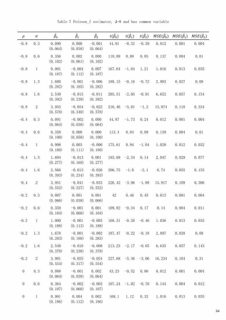
64
Table 7 Poisson_f estimator, 𝜆=8 and has common variable
𝜌 𝜎 ��0 ��1 ��2 𝑡(��0) 𝑡(��1) 𝑡(��2) 𝑀𝑆𝐸(��0) 𝑀𝑆𝐸(��1) 𝑀𝑆𝐸(��2)
-0.8 0.3 0.090
(0.064)
0.000
(0.038)
-0.001
(0.064)
44.91 -0.32 -0.39 0.012 0.001 0.004
-0.8 0.6 0.356
(0.102)
0.002
(0.061)
0.000
(0.102)
110.89 0.89 0.05 0.137 0.004 0.01
-0.8 1 0.991
(0.187)
-0.004
(0.112)
0.007
(0.187)
167.64 -1.04 1.21 1.016 0.013 0.035
-0.8 1.3 1.680
(0.282)
-0.001
(0.165)
-0.006
(0.282)
188.15 -0.16 -0.72 2.903 0.027 0.08
-0.8 1.6 2.549
(0.392)
-0.015
(0.239)
-0.011
(0.392)
205.51 -2.05 -0.91 6.652 0.057 0.154
-0.8 2 3.955
(0.578)
-0.054
(0.340)
-0.022
(0.578)
216.46 -5.01 -1.2 15.974 0.118 0.334
-0.4 0.3 0.091
(0.064)
-0.002
(0.038)
0.000
(0.064)
44.87 -1.73 0.24 0.012 0.001 0.004
-0.4 0.6 0.358
(0.100)
0.000
(0.059)
0.000
(0.100)
113.4 0.04 0.09 0.138 0.004 0.01
-0.4 1 0.998
(0.180)
0.003
(0.111)
-0.006
(0.180)
175.61 0.94 -1.04 1.028 0.012 0.032
-0.4 1.3 1.694
(0.277)
-0.013
(0.169)
0.001
(0.277)
193.69 -2.34 0.14 2.947 0.029 0.077
-0.4 1.6 2.566
(0.393)
-0.013
(0.234)
-0.026
(0.393)
206.75 -1.8 -2.1 6.74 0.055 0.155
-0.4 2 3.951
(0.552)
-0.041
(0.327)
-0.033
(0.552)
226.42 -3.96 -1.88 15.917 0.109 0.306
-0.2 0.3 0.087
(0.066)
0.001
(0.038)
0.001
(0.066)
42 0.46 0.45 0.012 0.001 0.004
-0.2 0.6 0.359
(0.104)
-0.001
(0.060)
0.001
(0.104)
109.82 -0.34 0.17 0.14 0.004 0.011
-0.2 1 1.000
(0.188)
-0.001
(0.113)
-0.003
(0.188)
168.31 -0.28 -0.46 1.036 0.013 0.035
-0.2 1.3 1.678
(0.283)
-0.001
(0.168)
-0.002
(0.283)
187.47 -0.22 -0.18 2.897 0.028 0.08
-0.2 1.6 2.548
(0.378)
-0.016
(0.238)
-0.008
(0.378)
213.23 -2.17 -0.65 6.635 0.057 0.143
-0.2 2 3.991
(0.554)
-0.055
(0.317)
-0.054
(0.554)
227.68 -5.46 -3.06 16.234 0.104 0.31
0 0.3 0.088
(0.064)
-0.001
(0.038)
0.002
(0.064)
43.23 -0.52 0.86 0.012 0.001 0.004
0 0.6 0.364
(0.107)
-0.002
(0.060)
-0.003
(0.107)
107.24 -1.02 -0.76 0.144 0.004 0.012
0 1 0.991
(0.186)
0.004
(0.112)
0.002
(0.186)
168.1 1.12 0.32 1.016 0.013 0.035
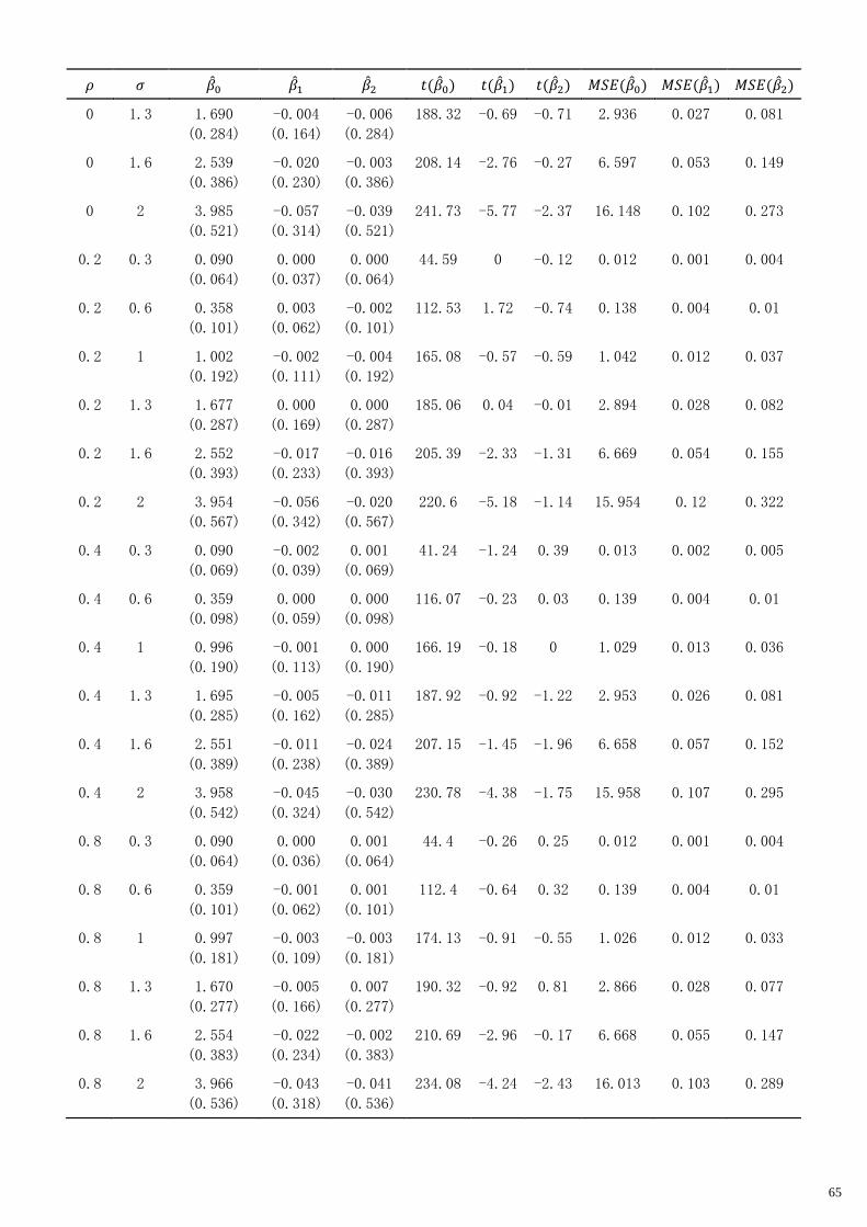
65
𝜌 𝜎 ��0 ��1 ��2 𝑡(��0) 𝑡(��1) 𝑡(��2) 𝑀𝑆𝐸(��0) 𝑀𝑆𝐸(��1) 𝑀𝑆𝐸(��2)
0 1.3 1.690
(0.284)
-0.004
(0.164)
-0.006
(0.284)
188.32 -0.69 -0.71 2.936 0.027 0.081
0 1.6 2.539
(0.386)
-0.020
(0.230)
-0.003
(0.386)
208.14 -2.76 -0.27 6.597 0.053 0.149
0 2 3.985
(0.521)
-0.057
(0.314)
-0.039
(0.521)
241.73 -5.77 -2.37 16.148 0.102 0.273
0.2 0.3 0.090
(0.064)
0.000
(0.037)
0.000
(0.064)
44.59 0 -0.12 0.012 0.001 0.004
0.2 0.6 0.358
(0.101)
0.003
(0.062)
-0.002
(0.101)
112.53 1.72 -0.74 0.138 0.004 0.01
0.2 1 1.002
(0.192)
-0.002
(0.111)
-0.004
(0.192)
165.08 -0.57 -0.59 1.042 0.012 0.037
0.2 1.3 1.677
(0.287)
0.000
(0.169)
0.000
(0.287)
185.06 0.04 -0.01 2.894 0.028 0.082
0.2 1.6 2.552
(0.393)
-0.017
(0.233)
-0.016
(0.393)
205.39 -2.33 -1.31 6.669 0.054 0.155
0.2 2 3.954
(0.567)
-0.056
(0.342)
-0.020
(0.567)
220.6 -5.18 -1.14 15.954 0.12 0.322
0.4 0.3 0.090
(0.069)
-0.002
(0.039)
0.001
(0.069)
41.24 -1.24 0.39 0.013 0.002 0.005
0.4 0.6 0.359
(0.098)
0.000
(0.059)
0.000
(0.098)
116.07 -0.23 0.03 0.139 0.004 0.01
0.4 1 0.996
(0.190)
-0.001
(0.113)
0.000
(0.190)
166.19 -0.18 0 1.029 0.013 0.036
0.4 1.3 1.695
(0.285)
-0.005
(0.162)
-0.011
(0.285)
187.92 -0.92 -1.22 2.953 0.026 0.081
0.4 1.6 2.551
(0.389)
-0.011
(0.238)
-0.024
(0.389)
207.15 -1.45 -1.96 6.658 0.057 0.152
0.4 2 3.958
(0.542)
-0.045
(0.324)
-0.030
(0.542)
230.78 -4.38 -1.75 15.958 0.107 0.295
0.8 0.3 0.090
(0.064)
0.000
(0.036)
0.001
(0.064)
44.4 -0.26 0.25 0.012 0.001 0.004
0.8 0.6 0.359
(0.101)
-0.001
(0.062)
0.001
(0.101)
112.4 -0.64 0.32 0.139 0.004 0.01
0.8 1 0.997
(0.181)
-0.003
(0.109)
-0.003
(0.181)
174.13 -0.91 -0.55 1.026 0.012 0.033
0.8 1.3 1.670
(0.277)
-0.005
(0.166)
0.007
(0.277)
190.32 -0.92 0.81 2.866 0.028 0.077
0.8 1.6 2.554
(0.383)
-0.022
(0.234)
-0.002
(0.383)
210.69 -2.96 -0.17 6.668 0.055 0.147
0.8 2 3.966
(0.536)
-0.043
(0.318)
-0.041
(0.536)
234.08 -4.24 -2.43 16.013 0.103 0.289
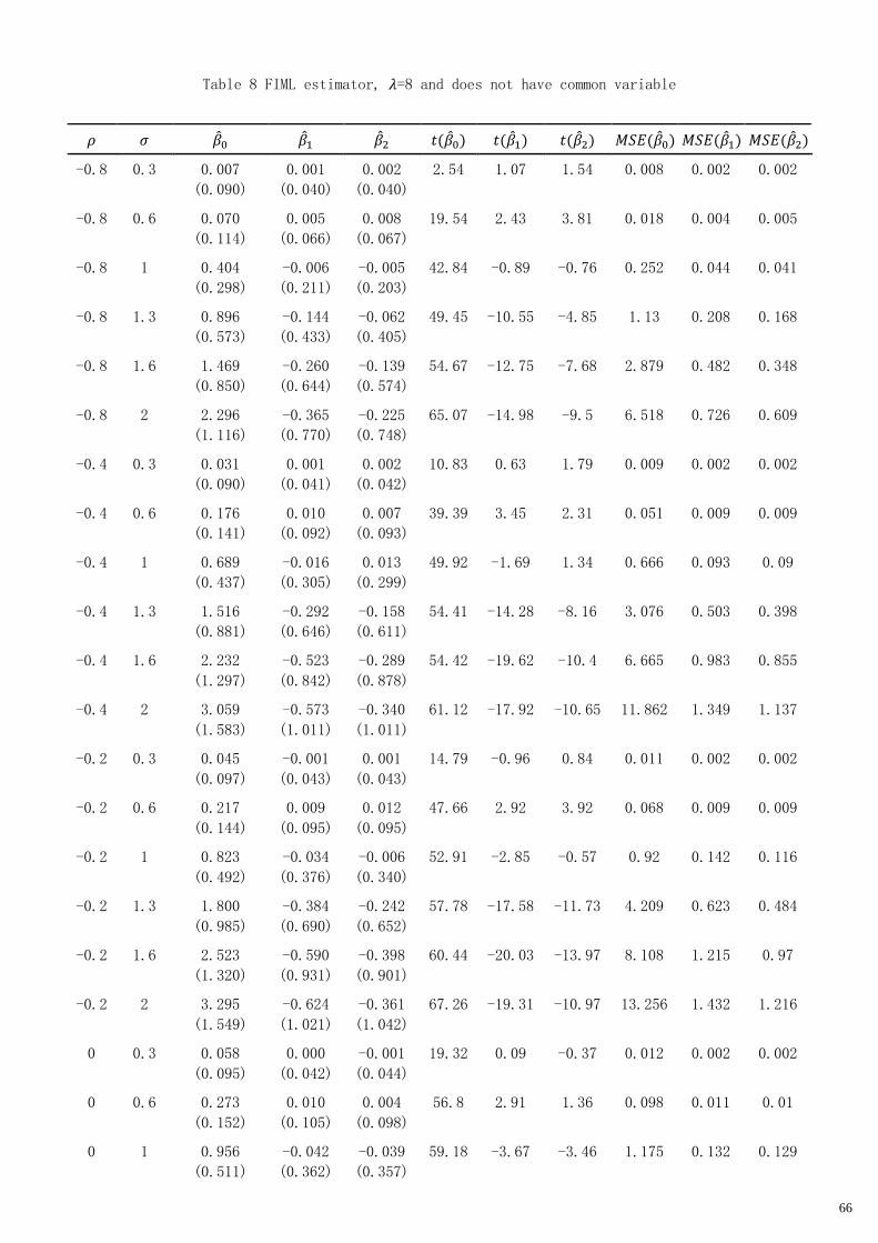
66
Table 8 FIML estimator, 𝜆=8 and does not have common variable
𝜌 𝜎 ��0 ��1 ��2 𝑡(��0) 𝑡(��1) 𝑡(��2) 𝑀𝑆𝐸(��0) 𝑀𝑆𝐸(��1) 𝑀𝑆𝐸(��2)
-0.8 0.3 0.007
(0.090)
0.001
(0.040)
0.002
(0.040)
2.54 1.07 1.54 0.008 0.002 0.002
-0.8 0.6 0.070
(0.114)
0.005
(0.066)
0.008
(0.067)
19.54 2.43 3.81 0.018 0.004 0.005
-0.8 1 0.404
(0.298)
-0.006
(0.211)
-0.005
(0.203)
42.84 -0.89 -0.76 0.252 0.044 0.041
-0.8 1.3 0.896
(0.573)
-0.144
(0.433)
-0.062
(0.405)
49.45 -10.55 -4.85 1.13 0.208 0.168
-0.8 1.6 1.469
(0.850)
-0.260
(0.644)
-0.139
(0.574)
54.67 -12.75 -7.68 2.879 0.482 0.348
-0.8 2 2.296
(1.116)
-0.365
(0.770)
-0.225
(0.748)
65.07 -14.98 -9.5 6.518 0.726 0.609
-0.4 0.3 0.031
(0.090)
0.001
(0.041)
0.002
(0.042)
10.83 0.63 1.79 0.009 0.002 0.002
-0.4 0.6 0.176
(0.141)
0.010
(0.092)
0.007
(0.093)
39.39 3.45 2.31 0.051 0.009 0.009
-0.4 1 0.689
(0.437)
-0.016
(0.305)
0.013
(0.299)
49.92 -1.69 1.34 0.666 0.093 0.09
-0.4 1.3 1.516
(0.881)
-0.292
(0.646)
-0.158
(0.611)
54.41 -14.28 -8.16 3.076 0.503 0.398
-0.4 1.6 2.232
(1.297)
-0.523
(0.842)
-0.289
(0.878)
54.42 -19.62 -10.4 6.665 0.983 0.855
-0.4 2 3.059
(1.583)
-0.573
(1.011)
-0.340
(1.011)
61.12 -17.92 -10.65 11.862 1.349 1.137
-0.2 0.3 0.045
(0.097)
-0.001
(0.043)
0.001
(0.043)
14.79 -0.96 0.84 0.011 0.002 0.002
-0.2 0.6 0.217
(0.144)
0.009
(0.095)
0.012
(0.095)
47.66 2.92 3.92 0.068 0.009 0.009
-0.2 1 0.823
(0.492)
-0.034
(0.376)
-0.006
(0.340)
52.91 -2.85 -0.57 0.92 0.142 0.116
-0.2 1.3 1.800
(0.985)
-0.384
(0.690)
-0.242
(0.652)
57.78 -17.58 -11.73 4.209 0.623 0.484
-0.2 1.6 2.523
(1.320)
-0.590
(0.931)
-0.398
(0.901)
60.44 -20.03 -13.97 8.108 1.215 0.97
-0.2 2 3.295
(1.549)
-0.624
(1.021)
-0.361
(1.042)
67.26 -19.31 -10.97 13.256 1.432 1.216
0 0.3 0.058
(0.095)
0.000
(0.042)
-0.001
(0.044)
19.32 0.09 -0.37 0.012 0.002 0.002
0 0.6 0.273
(0.152)
0.010
(0.105)
0.004
(0.098)
56.8 2.91 1.36 0.098 0.011 0.01
0 1 0.956
(0.511)
-0.042
(0.362)
-0.039
(0.357)
59.18 -3.67 -3.46 1.175 0.132 0.129
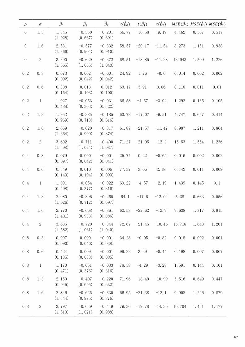
67
𝜌 𝜎 ��0 ��1 ��2 𝑡(��0) 𝑡(��1) 𝑡(��2) 𝑀𝑆𝐸(��0) 𝑀𝑆𝐸(��1) 𝑀𝑆𝐸(��2)
0 1.3 1.845
(1.028)
-0.350
(0.667)
-0.201
(0.691)
56.77 -16.58 -9.19 4.462 0.567 0.517
0 1.6 2.531
(1.366)
-0.577
(0.904)
-0.332
(0.910)
58.57 -20.17 -11.54 8.273 1.151 0.938
0 2 3.390
(1.565)
-0.629
(1.055)
-0.372
(1.043)
68.51 -18.85 -11.28 13.943 1.509 1.226
0.2 0.3 0.073
(0.092)
0.002
(0.042)
-0.001
(0.042)
24.92 1.26 -0.6 0.014 0.002 0.002
0.2 0.6 0.308
(0.154)
0.013
(0.103)
0.012
(0.100)
63.17 3.91 3.86 0.118 0.011 0.01
0.2 1 1.027
(0.488)
-0.053
(0.363)
-0.031
(0.322)
66.58 -4.57 -3.04 1.292 0.135 0.105
0.2 1.3 1.952
(0.969)
-0.385
(0.713)
-0.185
(0.616)
63.72 -17.07 -9.51 4.747 0.657 0.414
0.2 1.6 2.669
(1.364)
-0.620
(0.909)
-0.317
(0.874)
61.87 -21.57 -11.47 8.987 1.211 0.864
0.2 2 3.602
(1.598)
-0.711
(1.024)
-0.400
(1.037)
71.27 -21.95 -12.2 15.53 1.554 1.236
0.4 0.3 0.079
(0.097)
0.000
(0.042)
-0.001
(0.041)
25.74 0.22 -0.65 0.016 0.002 0.002
0.4 0.6 0.349
(0.143)
0.010
(0.104)
0.006
(0.093)
77.37 3.06 2.18 0.142 0.011 0.009
0.4 1 1.091
(0.498)
-0.054
(0.377)
-0.022
(0.316)
69.22 -4.57 -2.19 1.439 0.145 0.1
0.4 1.3 2.080
(1.026)
-0.396
(0.712)
-0.265
(0.697)
64.1 -17.6 -12.04 5.38 0.663 0.556
0.4 1.6 2.770
(1.401)
-0.668
(0.933)
-0.361
(0.886)
62.53 -22.62 -12.9 9.638 1.317 0.915
0.4 2 3.635
(1.582)
-0.720
(1.061)
-0.344
(1.040)
72.67 -21.45 -10.46 15.718 1.643 1.201
0.8 0.3 0.097
(0.090)
0.000
(0.040)
-0.001
(0.038)
34.28 -0.05 -0.82 0.018 0.002 0.001
0.8 0.6 0.424
(0.135)
0.009
(0.083)
-0.001
(0.085)
99.22 3.29 -0.44 0.198 0.007 0.007
0.8 1 1.170
(0.471)
-0.051
(0.376)
-0.033
(0.316)
78.58 -4.29 -3.28 1.591 0.144 0.101
0.8 1.3 2.150
(0.945)
-0.407
(0.695)
-0.220
(0.632)
71.96 -18.49 -10.99 5.516 0.649 0.447
0.8 1.6 2.846
(1.344)
-0.625
(0.925)
-0.335
(0.876)
66.95 -21.38 -12.1 9.908 1.246 0.879
0.8 2 3.797
(1.513)
-0.639
(1.021)
-0.449
(0.988)
79.36 -19.78 -14.36 16.704 1.451 1.177

68
Table 9 TSM estimator, 𝜆=8 and does not have common variable
𝜌 𝜎 ��0 ��1 ��2 𝑡(��0) 𝑡(��1) 𝑡(��2) 𝑀𝑆𝐸(��0) 𝑀𝑆𝐸(��1) 𝑀𝑆𝐸(��2)
-0.8 0.3 0.065
(0.178)
0.000
(0.045)
0.000
(0.046)
11.52 0.29 0.09 0.036 0.002 0.002
-0.8 0.6 0.307
(0.260)
0.008
(0.075)
0.010
(0.072)
37.36 3.23 4.46 0.162 0.006 0.005
-0.8 1 0.831
(0.482)
0.015
(0.125)
0.023
(0.126)
54.53 3.74 5.7 0.922 0.016 0.016
-0.8 1.3 1.230
(4.519)
0.108
(2.241)
0.031
(0.475)
8.61 1.52 2.1 21.936 5.035 0.227
-0.8 1.6 2.005
(2.068)
0.080
(1.243)
0.061
(0.650)
30.66 2.05 2.97 8.296 1.551 0.427
-0.8 2 2.472
(6.861)
0.275
(3.989)
0.119
(1.384)
11.39 2.18 2.72 53.187 15.989 1.931
-0.4 0.3 0.054
(0.168)
0.001
(0.046)
0.003
(0.047)
10.16 1.02 2.27 0.031 0.002 0.002
-0.4 0.6 0.339
(0.271)
0.003
(0.082)
0.003
(0.086)
39.52 1 0.92 0.188 0.007 0.007
-0.4 1 0.824
(4.987)
0.032
(0.526)
0.105
(2.588)
5.23 1.93 1.28 25.546 0.277 6.707
-0.4 1.3 1.365
(4.290)
0.123
(1.599)
0.116
(1.686)
10.06 2.43 2.18 20.265 2.572 2.856
-0.4 1.6 1.712
(10.153)
0.429
(3.941)
0.455
(4.735)
5.33 3.44 3.04 106.016 15.711 22.63
-0.4 2 2.402
(16.101)
0.557
(3.949)
0.780
(8.121)
4.72 4.46 3.04 264.996 15.907 66.562
-0.2 0.3 0.064
(0.159)
-0.001
(0.047)
0.002
(0.050)
12.66 -0.79 1.3 0.029 0.002 0.002
-0.2 0.6 0.340
(0.256)
0.002
(0.081)
0.006
(0.085)
41.92 0.84 2.16 0.181 0.007 0.007
-0.2 1 0.924
(2.636)
0.051
(1.054)
0.039
(0.654)
11.09 1.52 1.87 7.804 1.114 0.429
-0.2 1.3 1.527
(2.863)
0.166
(1.819)
0.099
(1.131)
16.87 2.88 2.76 10.531 3.337 1.289
-0.2 1.6 1.941
(13.240)
0.438
(5.466)
0.219
(4.979)
4.64 2.54 1.39 179.073 30.07 24.839
-0.2 2 2.476
(23.136)
0.160
(2.844)
1.163
(11.880)
3.38 1.78 3.1 541.424 8.114 142.486
0 0.3 0.061
(0.157)
0.000
(0.047)
0.003
(0.051)
12.29 0.27 1.68 0.029 0.002 0.003
0 0.6 0.348
(0.232)
0.004
(0.086)
0.003
(0.080)
47.28 1.31 1.23 0.175 0.007 0.006
0 1 0.784
(5.445)
0.134
(2.737)
0.089
(1.232)
4.55 1.55 2.27 30.266 7.508 1.525
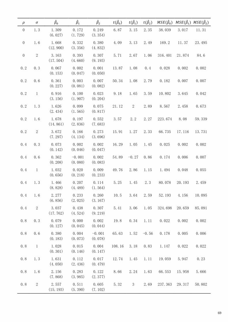
69
𝜌 𝜎 ��0 ��1 ��2 𝑡(��0) 𝑡(��1) 𝑡(��2) 𝑀𝑆𝐸(��0) 𝑀𝑆𝐸(��1) 𝑀𝑆𝐸(��2)
0 1.3 1.309
(6.027)
0.172
(1.729)
0.249
(3.354)
6.87 3.15 2.35 38.039 3.017 11.31
0 1.6 1.668
(12.900)
0.332
(3.356)
0.380
(4.832)
4.09 3.13 2.49 169.2 11.37 23.495
0 2 3.163
(17.504)
0.393
(4.660)
0.307
(9.193)
5.71 2.67 1.06 316.401 21.874 84.6
0.2 0.3 0.067
(0.153)
0.002
(0.047)
0.001
(0.050)
13.87 1.08 0.4 0.028 0.002 0.002
0.2 0.6 0.361
(0.227)
0.003
(0.081)
0.007
(0.082)
50.34 1.08 2.79 0.182 0.007 0.007
0.2 1 0.916
(3.156)
0.100
(1.907)
0.023
(0.204)
9.18 1.65 3.59 10.802 3.645 0.042
0.2 1.3 1.626
(2.434)
0.099
(1.565)
0.075
(0.817)
21.12 2 2.89 8.567 2.458 0.673
0.2 1.6 1.678
(14.861)
0.197
(2.836)
0.552
(7.683)
3.57 2.2 2.27 223.674 8.08 59.339
0.2 2 3.672
(7.297)
0.166
(4.134)
0.273
(3.696)
15.91 1.27 2.33 66.735 17.116 13.731
0.4 0.3 0.073
(0.142)
0.002
(0.046)
0.002
(0.047)
16.29 1.05 1.45 0.025 0.002 0.002
0.4 0.6 0.362
(0.208)
-0.001
(0.080)
0.002
(0.083)
54.89 -0.27 0.86 0.174 0.006 0.007
0.4 1 1.032
(0.656)
0.020
(0.218)
0.009
(0.233)
49.76 2.86 1.15 1.494 0.048 0.055
0.4 1.3 1.466
(8.828)
0.207
(4.489)
0.114
(1.564)
5.25 1.45 2.3 80.078 20.193 2.459
0.4 1.6 2.277
(6.856)
0.233
(2.025)
0.260
(3.167)
10.5 3.64 2.59 52.193 4.156 10.095
0.4 2 3.037
(17.762)
0.438
(4.524)
0.307
(9.219)
5.41 3.06 1.05 324.698 20.659 85.091
0.8 0.3 0.079
(0.127)
0.000
(0.045)
0.002
(0.044)
19.8 0.34 1.11 0.022 0.002 0.002
0.8 0.6 0.380
(0.183)
0.004
(0.073)
-0.001
(0.078)
65.63 1.52 -0.56 0.178 0.005 0.006
0.8 1 1.028
(0.301)
0.015
(0.146)
0.004
(0.147)
108.16 3.18 0.83 1.147 0.022 0.022
0.8 1.3 1.631
(4.050)
0.112
(2.436)
0.017
(0.479)
12.74 1.45 1.11 19.059 5.947 0.23
0.8 1.6 2.156
(7.868)
0.283
(3.985)
0.122
(2.377)
8.66 2.24 1.63 66.553 15.958 5.666
0.8 2 2.557
(15.193)
0.511
(5.390)
0.605
(7.102)
5.32 3 2.69 237.363 29.317 50.802
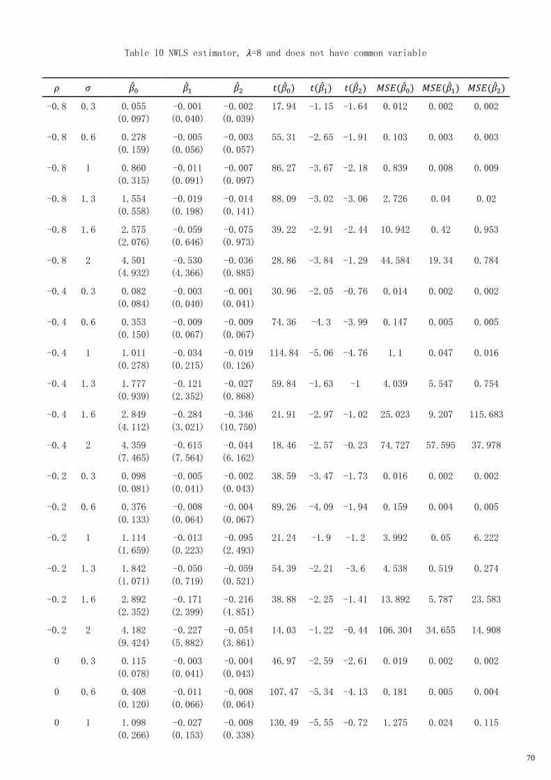
70
Table 10 NWLS estimator, 𝜆=8 and does not have common variable
𝜌 𝜎 ��0 ��1 ��2 𝑡(��0) 𝑡(��1) 𝑡(��2) 𝑀𝑆𝐸(��0) 𝑀𝑆𝐸(��1) 𝑀𝑆𝐸(��2)
-0.8 0.3 0.055
(0.097)
-0.001
(0.040)
-0.002
(0.039)
17.94 -1.15 -1.64 0.012 0.002 0.002
-0.8 0.6 0.278
(0.159)
-0.005
(0.056)
-0.003
(0.057)
55.31 -2.65 -1.91 0.103 0.003 0.003
-0.8 1 0.860
(0.315)
-0.011
(0.091)
-0.007
(0.097)
86.27 -3.67 -2.18 0.839 0.008 0.009
-0.8 1.3 1.554
(0.558)
-0.019
(0.198)
-0.014
(0.141)
88.09 -3.02 -3.06 2.726 0.04 0.02
-0.8 1.6 2.575
(2.076)
-0.059
(0.646)
-0.075
(0.973)
39.22 -2.91 -2.44 10.942 0.42 0.953
-0.8 2 4.501
(4.932)
-0.530
(4.366)
-0.036
(0.885)
28.86 -3.84 -1.29 44.584 19.34 0.784
-0.4 0.3 0.082
(0.084)
-0.003
(0.040)
-0.001
(0.041)
30.96 -2.05 -0.76 0.014 0.002 0.002
-0.4 0.6 0.353
(0.150)
-0.009
(0.067)
-0.009
(0.067)
74.36 -4.3 -3.99 0.147 0.005 0.005
-0.4 1 1.011
(0.278)
-0.034
(0.215)
-0.019
(0.126)
114.84 -5.06 -4.76 1.1 0.047 0.016
-0.4 1.3 1.777
(0.939)
-0.121
(2.352)
-0.027
(0.868)
59.84 -1.63 -1 4.039 5.547 0.754
-0.4 1.6 2.849
(4.112)
-0.284
(3.021)
-0.346
(10.750)
21.91 -2.97 -1.02 25.023 9.207 115.683
-0.4 2 4.359
(7.465)
-0.615
(7.564)
-0.044
(6.162)
18.46 -2.57 -0.23 74.727 57.595 37.978
-0.2 0.3 0.098
(0.081)
-0.005
(0.041)
-0.002
(0.043)
38.59 -3.47 -1.73 0.016 0.002 0.002
-0.2 0.6 0.376
(0.133)
-0.008
(0.064)
-0.004
(0.067)
89.26 -4.09 -1.94 0.159 0.004 0.005
-0.2 1 1.114
(1.659)
-0.013
(0.223)
-0.095
(2.493)
21.24 -1.9 -1.2 3.992 0.05 6.222
-0.2 1.3 1.842
(1.071)
-0.050
(0.719)
-0.059
(0.521)
54.39 -2.21 -3.6 4.538 0.519 0.274
-0.2 1.6 2.892
(2.352)
-0.171
(2.399)
-0.216
(4.851)
38.88 -2.25 -1.41 13.892 5.787 23.583
-0.2 2 4.182
(9.424)
-0.227
(5.882)
-0.054
(3.861)
14.03 -1.22 -0.44 106.304 34.655 14.908
0 0.3 0.115
(0.078)
-0.003
(0.041)
-0.004
(0.043)
46.97 -2.59 -2.61 0.019 0.002 0.002
0 0.6 0.408
(0.120)
-0.011
(0.066)
-0.008
(0.064)
107.47 -5.34 -4.13 0.181 0.005 0.004
0 1 1.098
(0.266)
-0.027
(0.153)
-0.008
(0.338)
130.49 -5.55 -0.72 1.275 0.024 0.115

71
𝜌 𝜎 ��0 ��1 ��2 𝑡(��0) 𝑡(��1) 𝑡(��2) 𝑀𝑆𝐸(��0) 𝑀𝑆𝐸(��1) 𝑀𝑆𝐸(��2)
0 1.3 2.002
(1.689)
-0.174
(1.789)
-0.046
(0.852)
37.48 -3.07 -1.72 6.861 3.23 0.728
0 1.6 3.201
(5.000)
-0.223
(2.797)
-0.200
(3.920)
20.24 -2.52 -1.62 35.246 7.874 15.405
0 2 4.564
(3.473)
-0.988
(12.315)
-0.134
(2.431)
41.55 -2.54 -1.74 32.894 152.647 5.927
0.2 0.3 0.128
(0.074)
-0.001
(0.042)
-0.004
(0.042)
54.92 -1.1 -3.07 0.022 0.002 0.002
0.2 0.6 0.438
(0.115)
-0.009
(0.064)
-0.007
(0.063)
120.51 -4.57 -3.27 0.205 0.004 0.004
0.2 1 1.160
(0.311)
-0.059
(1.195)
-0.014
(0.120)
118.07 -1.57 -3.81 1.443 1.431 0.015
0.2 1.3 2.005
(1.812)
-0.128
(1.941)
-0.053
(0.544)
34.99 -2.09 -3.06 7.3 3.783 0.299
0.2 1.6 3.118
(2.922)
-0.566
(6.702)
0.034
(2.065)
33.75 -2.67 0.52 18.262 45.243 4.265
0.2 2 4.529
(3.516)
-0.322
(4.436)
-0.393
(12.787)
40.73 -2.3 -0.97 32.872 19.781 163.67
0.4 0.3 0.145
(0.073)
-0.003
(0.041)
-0.004
(0.041)
62.64 -2.33 -2.87 0.026 0.002 0.002
0.4 0.6 0.468
(0.109)
-0.010
(0.063)
-0.009
(0.065)
135.95 -5.25 -4.42 0.231 0.004 0.004
0.4 1 1.194
(0.210)
-0.025
(0.121)
-0.028
(0.115)
179.66 -6.47 -7.82 1.469 0.015 0.014
0.4 1.3 1.973
(0.397)
0.000
(1.470)
-0.038
(0.221)
157.31 0 -5.45 4.05 2.162 0.05
0.4 1.6 2.965
(1.326)
-0.115
(1.086)
-0.193
(3.620)
70.7 -3.35 -1.68 10.55 1.192 13.142
0.4 2 5.058
(5.438)
-0.619
(6.130)
-0.281
(3.028)
29.41 -3.2 -2.94 55.161 37.955 9.249
0.8 0.3 0.175
(0.066)
-0.004
(0.040)
-0.004
(0.038)
84.09 -3.4 -3.49 0.035 0.002 0.001
0.8 0.6 0.517
(0.097)
-0.010
(0.056)
-0.012
(0.061)
169.14 -5.42 -6.09 0.277 0.003 0.004
0.8 1 1.224
(0.175)
-0.019
(0.105)
-0.020
(0.109)
220.95 -5.65 -5.92 1.53 0.011 0.012
0.8 1.3 2.015
(0.316)
-0.044
(0.315)
-0.045
(0.198)
201.91 -4.38 -7.16 4.162 0.101 0.041
0.8 1.6 3.029
(1.158)
-0.131
(2.710)
-0.136
(1.536)
82.7 -1.53 -2.79 10.517 7.362 2.376
0.8 2 4.760
(4.426)
-0.189
(3.442)
-0.426
(6.251)
34.01 -1.74 -2.16 42.246 11.884 39.259

72
Table 11 Poisson_s estimator, 𝜆=8 and does not have common variable
𝜌 𝜎 ��0 ��1 ��2 𝑡(��0) 𝑡(��1) 𝑡(��2) 𝑀𝑆𝐸(��0) 𝑀𝑆𝐸(��1) 𝑀𝑆𝐸(��2)
-0.8 0.3 -0.015
(0.068)
0.001
(0.040)
0.003
(0.040)
-6.78 1.07 1.99 0.005 0.002 0.002
-0.8 0.6 0.116
(0.095)
0.004
(0.059)
0.009
(0.059)
38.57 2.16 4.82 0.023 0.003 0.004
-0.8 1 0.521
(0.156)
0.009
(0.094)
0.018
(0.094)
105.68 3.1 6.19 0.296 0.009 0.009
-0.8 1.3 1.011
(0.197)
0.006
(0.124)
0.017
(0.124)
162.25 1.66 4.44 1.06 0.015 0.016
-0.8 1.6 1.641
(0.266)
0.001
(0.167)
0.016
(0.167)
194.94 0.25 3.09 2.764 0.028 0.028
-0.8 2 2.681
(0.387)
0.002
(0.231)
0.015
(0.231)
218.93 0.21 2.01 7.337 0.054 0.054
-0.4 0.3 0.037
(0.067)
0.001
(0.040)
0.003
(0.040)
17.59 0.71 2.5 0.006 0.002 0.002
-0.4 0.6 0.259
(0.110)
0.000
(0.068)
0.001
(0.068)
74.46 -0.14 0.42 0.079 0.005 0.005
-0.4 1 0.806
(0.189)
-0.004
(0.119)
0.008
(0.119)
135.01 -1.15 2.22 0.685 0.014 0.014
-0.4 1.3 1.427
(0.276)
-0.006
(0.177)
0.000
(0.177)
163.67 -1.04 0.07 2.114 0.031 0.031
-0.4 1.6 2.208
(0.393)
-0.015
(0.228)
0.001
(0.228)
177.47 -2.05 0.16 5.032 0.052 0.052
-0.4 2 3.515
(0.548)
-0.034
(0.346)
-0.016
(0.346)
202.75 -3.14 -1.43 12.655 0.121 0.12
-0.2 0.3 0.067
(0.069)
-0.002
(0.041)
0.001
(0.041)
30.66 -1.24 0.98 0.009 0.002 0.002
-0.2 0.6 0.312
(0.112)
-0.001
(0.067)
0.003
(0.067)
87.79 -0.29 1.51 0.11 0.004 0.004
-0.2 1 0.903
(0.200)
0.004
(0.122)
0.004
(0.122)
143.03 1.08 1.09 0.855 0.015 0.015
-0.2 1.3 1.563
(0.302)
-0.002
(0.184)
0.001
(0.184)
163.88 -0.27 0.25 2.534 0.034 0.034
-0.2 1.6 2.398
(0.415)
-0.008
(0.253)
-0.003
(0.253)
182.73 -0.96 -0.36 5.924 0.064 0.064
-0.2 2 3.819
(0.591)
-0.071
(0.349)
-0.043
(0.349)
204.26 -6.4 -3.9 14.935 0.127 0.124
0 0.3 0.090
(0.069)
0.000
(0.041)
0.000
(0.041)
41.33 -0.1 0.12 0.013 0.002 0.002
0 0.6 0.362
(0.109)
-0.002
(0.070)
-0.001
(0.070)
104.64 -1 -0.51 0.143 0.005 0.005
0 1 0.989
(0.206)
0.003
(0.131)
0.001
(0.131)
152.07 0.69 0.33 1.021 0.017 0.017

73
𝜌 𝜎 ��0 ��1 ��2 𝑡(��0) 𝑡(��1) 𝑡(��2) 𝑀𝑆𝐸(��0) 𝑀𝑆𝐸(��1) 𝑀𝑆𝐸(��2)
0 1.3 1.674
(0.293)
-0.008
(0.184)
0.005
(0.184)
180.8 -1.38 0.91 2.887 0.034 0.034
0 1.6 2.558
(0.428)
-0.027
(0.252)
-0.018
(0.252)
189.07 -3.41 -2.26 6.727 0.064 0.064
0 2 4.005
(0.589)
-0.078
(0.357)
-0.051
(0.357)
215.1 -6.93 -4.55 16.386 0.134 0.13
0.2 0.3 0.109
(0.069)
0.001
(0.041)
-0.001
(0.041)
50.11 1.02 -0.87 0.017 0.002 0.002
0.2 0.6 0.403
(0.108)
-0.002
(0.067)
0.001
(0.067)
118.34 -0.96 0.4 0.174 0.004 0.004
0.2 1 1.052
(0.198)
0.003
(0.125)
0.005
(0.125)
168.41 0.66 1.17 1.146 0.016 0.016
0.2 1.3 1.756
(0.282)
-0.009
(0.179)
0.003
(0.179)
196.93 -1.51 0.54 3.164 0.032 0.032
0.2 1.6 2.681
(0.416)
-0.034
(0.247)
-0.035
(0.247)
203.86 -4.41 -4.47 7.361 0.062 0.062
0.2 2 4.102
(0.555)
-0.062
(0.338)
-0.057
(0.338)
233.63 -5.79 -5.37 17.133 0.118 0.117
0.4 0.3 0.131
(0.070)
0.000
(0.041)
-0.001
(0.041)
59.47 0.34 -0.6 0.022 0.002 0.002
0.4 0.6 0.444
(0.105)
-0.004
(0.066)
-0.004
(0.066)
134.03 -2.08 -1.81 0.208 0.004 0.004
0.4 1 1.123
(0.193)
-0.002
(0.122)
-0.010
(0.122)
184.06 -0.42 -2.69 1.298 0.015 0.015
0.4 1.3 1.845
(0.279)
-0.017
(0.175)
-0.011
(0.175)
208.94 -3.1 -2.01 3.483 0.031 0.031
0.4 1.6 2.708
(0.386)
-0.010
(0.246)
-0.017
(0.246)
221.57 -1.26 -2.16 7.482 0.061 0.061
0.4 2 4.206
(0.536)
-0.076
(0.326)
-0.066
(0.326)
248.23 -7.37 -6.35 17.98 0.112 0.111
0.8 0.3 0.169
(0.064)
-0.001
(0.040)
-0.002
(0.040)
82.94 -0.46 -1.58 0.033 0.002 0.002
0.8 0.6 0.503
(0.101)
-0.002
(0.060)
-0.008
(0.060)
157.38 -1.15 -4.25 0.263 0.004 0.004
0.8 1 1.185
(0.179)
0.000
(0.114)
-0.009
(0.114)
209 -0.09 -2.64 1.436 0.013 0.013
0.8 1.3 1.923
(0.263)
-0.010
(0.163)
-0.021
(0.163)
230.77 -1.89 -4.14 3.766 0.027 0.027
0.8 1.6 2.808
(0.369)
-0.030
(0.224)
-0.032
(0.224)
240.93 -4.29 -4.57 8.02 0.051 0.051
0.8 2 4.218
(0.518)
-0.056
(0.311)
-0.050
(0.311)
257.55 -5.65 -5.1 18.06 0.1 0.1
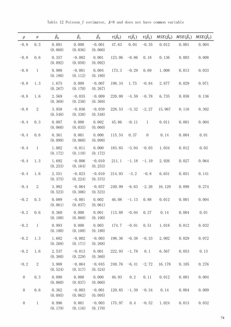
74
Table 12 Poisson_f estimator, 𝜆=8 and does not have common variable
𝜌 𝜎 ��0 ��1 ��2 𝑡(��0) 𝑡(��1) 𝑡(��2) 𝑀𝑆𝐸(��0) 𝑀𝑆𝐸(��1) 𝑀𝑆𝐸(��2)
-0.8 0.3 0.091
(0.060)
0.000
(0.036)
-0.001
(0.060)
47.63 0.04 -0.35 0.012 0.001 0.004
-0.8 0.6 0.357
(0.092)
-0.002
(0.058)
0.001
(0.092)
123.06 -0.86 0.18 0.136 0.003 0.008
-0.8 1 0.988
(0.180)
-0.001
(0.112)
0.004
(0.180)
173.3 -0.29 0.69 1.008 0.013 0.033
-0.8 1.3 1.675
(0.267)
0.009
(0.170)
-0.007
(0.267)
198.34 1.75 -0.84 2.877 0.029 0.071
-0.8 1.6 2.569
(0.369)
-0.035
(0.238)
-0.009
(0.369)
220.08 -4.59 -0.78 6.735 0.058 0.136
-0.8 2 3.958
(0.548)
-0.036
(0.338)
-0.039
(0.548)
228.53 -3.32 -2.27 15.967 0.116 0.302
-0.4 0.3 0.087
(0.060)
0.000
(0.035)
0.002
(0.060)
45.86 -0.11 1 0.011 0.001 0.004
-0.4 0.6 0.361
(0.099)
0.001
(0.060)
0.000
(0.099)
115.54 0.37 0 0.14 0.004 0.01
-0.4 1 1.002
(0.172)
-0.011
(0.110)
0.000
(0.172)
183.85 -3.04 -0.03 1.034 0.012 0.03
-0.4 1.3 1.692
(0.253)
-0.006
(0.164)
-0.010
(0.253)
211.1 -1.18 -1.19 2.926 0.027 0.064
-0.4 1.6 2.551
(0.375)
-0.023
(0.224)
-0.010
(0.375)
214.93 -3.2 -0.8 6.651 0.051 0.141
-0.4 2 3.982
(0.523)
-0.064
(0.306)
-0.037
(0.523)
240.99 -6.63 -2.26 16.129 0.098 0.274
-0.2 0.3 0.089
(0.061)
-0.001
(0.037)
0.002
(0.061)
46.08 -1.13 0.88 0.012 0.001 0.004
-0.2 0.6 0.360
(0.100)
0.000
(0.060)
0.001
(0.100)
113.88 -0.04 0.27 0.14 0.004 0.01
-0.2 1 0.993
(0.180)
0.000
(0.108)
0.003
(0.180)
174.7 -0.01 0.51 1.018 0.012 0.032
-0.2 1.3 1.682
(0.268)
-0.002
(0.171)
-0.003
(0.268)
198.36 -0.38 -0.33 2.902 0.029 0.072
-0.2 1.6 2.537
(0.360)
-0.013
(0.229)
0.001
(0.360)
222.93 -1.78 0.1 6.567 0.053 0.13
-0.2 2 3.988
(0.524)
-0.064
(0.317)
-0.045
(0.524)
240.76 -6.41 -2.72 16.178 0.105 0.276
0 0.3 0.090
(0.060)
0.000
(0.037)
0.000
(0.060)
46.93 0.2 0.11 0.012 0.001 0.004
0 0.6 0.362
(0.095)
-0.003
(0.062)
-0.001
(0.095)
120.85 -1.39 -0.34 0.14 0.004 0.009
0 1 0.996
(0.179)
0.001
(0.116)
-0.003
(0.179)
175.97 0.4 -0.52 1.024 0.013 0.032
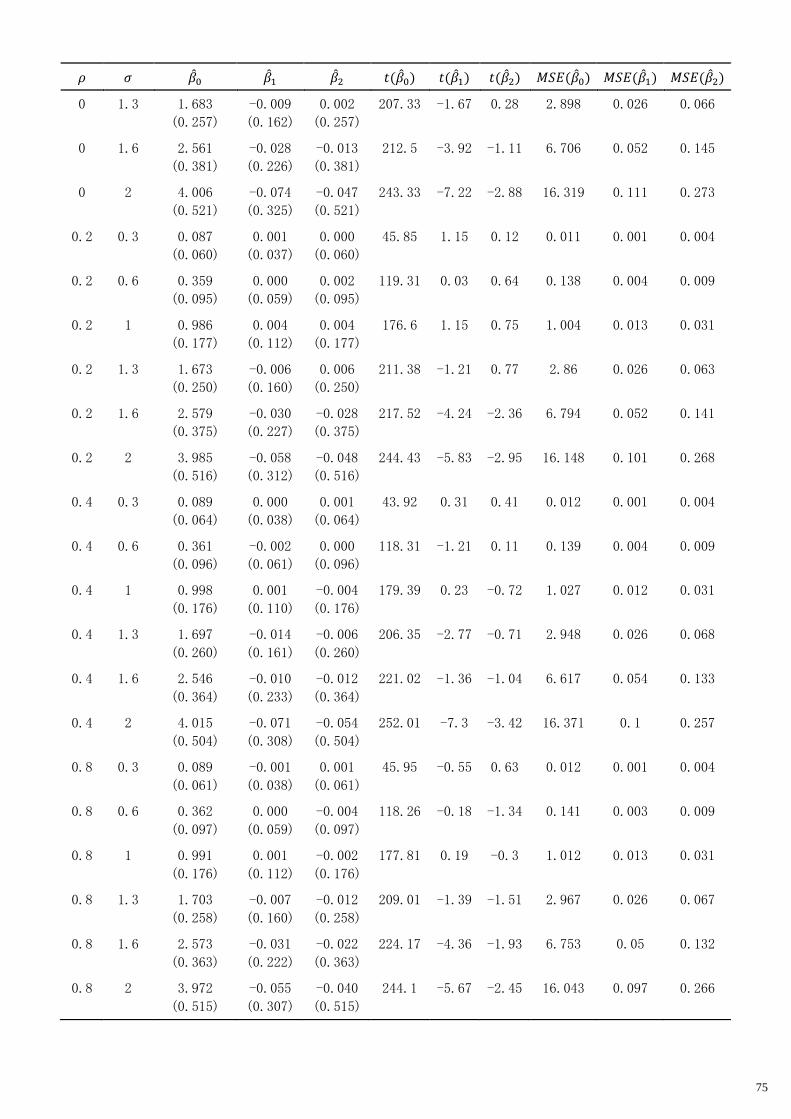
75
𝜌 𝜎 ��0 ��1 ��2 𝑡(��0) 𝑡(��1) 𝑡(��2) 𝑀𝑆𝐸(��0) 𝑀𝑆𝐸(��1) 𝑀𝑆𝐸(��2)
0 1.3 1.683
(0.257)
-0.009
(0.162)
0.002
(0.257)
207.33 -1.67 0.28 2.898 0.026 0.066
0 1.6 2.561
(0.381)
-0.028
(0.226)
-0.013
(0.381)
212.5 -3.92 -1.11 6.706 0.052 0.145
0 2 4.006
(0.521)
-0.074
(0.325)
-0.047
(0.521)
243.33 -7.22 -2.88 16.319 0.111 0.273
0.2 0.3 0.087
(0.060)
0.001
(0.037)
0.000
(0.060)
45.85 1.15 0.12 0.011 0.001 0.004
0.2 0.6 0.359
(0.095)
0.000
(0.059)
0.002
(0.095)
119.31 0.03 0.64 0.138 0.004 0.009
0.2 1 0.986
(0.177)
0.004
(0.112)
0.004
(0.177)
176.6 1.15 0.75 1.004 0.013 0.031
0.2 1.3 1.673
(0.250)
-0.006
(0.160)
0.006
(0.250)
211.38 -1.21 0.77 2.86 0.026 0.063
0.2 1.6 2.579
(0.375)
-0.030
(0.227)
-0.028
(0.375)
217.52 -4.24 -2.36 6.794 0.052 0.141
0.2 2 3.985
(0.516)
-0.058
(0.312)
-0.048
(0.516)
244.43 -5.83 -2.95 16.148 0.101 0.268
0.4 0.3 0.089
(0.064)
0.000
(0.038)
0.001
(0.064)
43.92 0.31 0.41 0.012 0.001 0.004
0.4 0.6 0.361
(0.096)
-0.002
(0.061)
0.000
(0.096)
118.31 -1.21 0.11 0.139 0.004 0.009
0.4 1 0.998
(0.176)
0.001
(0.110)
-0.004
(0.176)
179.39 0.23 -0.72 1.027 0.012 0.031
0.4 1.3 1.697
(0.260)
-0.014
(0.161)
-0.006
(0.260)
206.35 -2.77 -0.71 2.948 0.026 0.068
0.4 1.6 2.546
(0.364)
-0.010
(0.233)
-0.012
(0.364)
221.02 -1.36 -1.04 6.617 0.054 0.133
0.4 2 4.015
(0.504)
-0.071
(0.308)
-0.054
(0.504)
252.01 -7.3 -3.42 16.371 0.1 0.257
0.8 0.3 0.089
(0.061)
-0.001
(0.038)
0.001
(0.061)
45.95 -0.55 0.63 0.012 0.001 0.004
0.8 0.6 0.362
(0.097)
0.000
(0.059)
-0.004
(0.097)
118.26 -0.18 -1.34 0.141 0.003 0.009
0.8 1 0.991
(0.176)
0.001
(0.112)
-0.002
(0.176)
177.81 0.19 -0.3 1.012 0.013 0.031
0.8 1.3 1.703
(0.258)
-0.007
(0.160)
-0.012
(0.258)
209.01 -1.39 -1.51 2.967 0.026 0.067
0.8 1.6 2.573
(0.363)
-0.031
(0.222)
-0.022
(0.363)
224.17 -4.36 -1.93 6.753 0.05 0.132
0.8 2 3.972
(0.515)
-0.055
(0.307)
-0.040
(0.515)
244.1 -5.67 -2.45 16.043 0.097 0.266
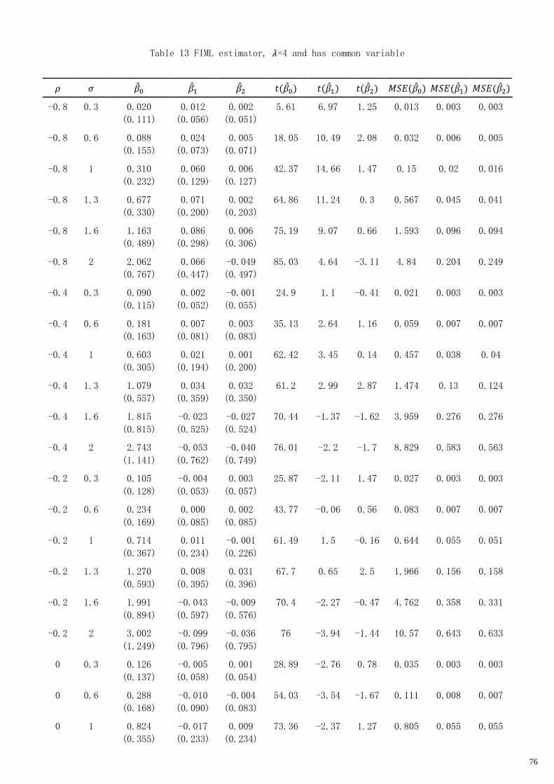
76
Table 13 FIML estimator, 𝜆=4 and has common variable
𝜌 𝜎 ��0 ��1 ��2 𝑡(��0) 𝑡(��1) 𝑡(��2) 𝑀𝑆𝐸(��0) 𝑀𝑆𝐸(��1) 𝑀𝑆𝐸(��2)
-0.8 0.3 0.020
(0.111)
0.012
(0.056)
0.002
(0.051)
5.61 6.97 1.25 0.013 0.003 0.003
-0.8 0.6 0.088
(0.155)
0.024
(0.073)
0.005
(0.071)
18.05 10.49 2.08 0.032 0.006 0.005
-0.8 1 0.310
(0.232)
0.060
(0.129)
0.006
(0.127)
42.37 14.66 1.47 0.15 0.02 0.016
-0.8 1.3 0.677
(0.330)
0.071
(0.200)
0.002
(0.203)
64.86 11.24 0.3 0.567 0.045 0.041
-0.8 1.6 1.163
(0.489)
0.086
(0.298)
0.006
(0.306)
75.19 9.07 0.66 1.593 0.096 0.094
-0.8 2 2.062
(0.767)
0.066
(0.447)
-0.049
(0.497)
85.03 4.64 -3.11 4.84 0.204 0.249
-0.4 0.3 0.090
(0.115)
0.002
(0.052)
-0.001
(0.055)
24.9 1.1 -0.41 0.021 0.003 0.003
-0.4 0.6 0.181
(0.163)
0.007
(0.081)
0.003
(0.083)
35.13 2.64 1.16 0.059 0.007 0.007
-0.4 1 0.603
(0.305)
0.021
(0.194)
0.001
(0.200)
62.42 3.45 0.14 0.457 0.038 0.04
-0.4 1.3 1.079
(0.557)
0.034
(0.359)
0.032
(0.350)
61.2 2.99 2.87 1.474 0.13 0.124
-0.4 1.6 1.815
(0.815)
-0.023
(0.525)
-0.027
(0.524)
70.44 -1.37 -1.62 3.959 0.276 0.276
-0.4 2 2.743
(1.141)
-0.053
(0.762)
-0.040
(0.749)
76.01 -2.2 -1.7 8.829 0.583 0.563
-0.2 0.3 0.105
(0.128)
-0.004
(0.053)
0.003
(0.057)
25.87 -2.11 1.47 0.027 0.003 0.003
-0.2 0.6 0.234
(0.169)
0.000
(0.085)
0.002
(0.085)
43.77 -0.06 0.56 0.083 0.007 0.007
-0.2 1 0.714
(0.367)
0.011
(0.234)
-0.001
(0.226)
61.49 1.5 -0.16 0.644 0.055 0.051
-0.2 1.3 1.270
(0.593)
0.008
(0.395)
0.031
(0.396)
67.7 0.65 2.5 1.966 0.156 0.158
-0.2 1.6 1.991
(0.894)
-0.043
(0.597)
-0.009
(0.576)
70.4 -2.27 -0.47 4.762 0.358 0.331
-0.2 2 3.002
(1.249)
-0.099
(0.796)
-0.036
(0.795)
76 -3.94 -1.44 10.57 0.643 0.633
0 0.3 0.126
(0.137)
-0.005
(0.058)
0.001
(0.054)
28.89 -2.76 0.78 0.035 0.003 0.003
0 0.6 0.288
(0.168)
-0.010
(0.090)
-0.004
(0.083)
54.03 -3.54 -1.67 0.111 0.008 0.007
0 1 0.824
(0.355)
-0.017
(0.233)
0.009
(0.234)
73.36 -2.37 1.27 0.805 0.055 0.055

77
𝜌 𝜎 ��0 ��1 ��2 𝑡(��0) 𝑡(��1) 𝑡(��2) 𝑀𝑆𝐸(��0) 𝑀𝑆𝐸(��1) 𝑀𝑆𝐸(��2)
0 1.3 1.405
(0.572)
-0.003
(0.388)
0.026
(0.398)
77.75 -0.25 2.04 2.301 0.151 0.159
0 1.6 2.175
(0.904)
-0.066
(0.575)
-0.004
(0.580)
76.07 -3.61 -0.2 5.55 0.335 0.336
0 2 3.274
(1.305)
-0.160
(0.832)
-0.069
(0.800)
79.34 -6.08 -2.72 12.424 0.717 0.645
0.2 0.3 0.158
(0.139)
-0.014
(0.054)
-0.004
(0.054)
36.04 -8.2 -2.22 0.044 0.003 0.003
0.2 0.6 0.326
(0.171)
-0.020
(0.088)
-0.005
(0.085)
60.4 -7.06 -1.69 0.135 0.008 0.007
0.2 1 0.887
(0.354)
-0.020
(0.228)
0.025
(0.226)
79.13 -2.75 3.56 0.912 0.053 0.052
0.2 1.3 1.518
(0.626)
-0.012
(0.411)
0.025
(0.401)
76.74 -0.95 1.94 2.695 0.169 0.161
0.2 1.6 2.365
(0.896)
-0.087
(0.562)
-0.060
(0.578)
83.45 -4.88 -3.26 6.399 0.323 0.338
0.2 2 3.407
(1.262)
-0.171
(0.790)
-0.066
(0.782)
85.36 -6.84 -2.68 13.204 0.653 0.615
0.4 0.3 0.164
(0.135)
-0.013
(0.051)
0.001
(0.052)
38.43 -7.8 0.58 0.045 0.003 0.003
0.4 0.6 0.382
(0.166)
-0.031
(0.079)
-0.004
(0.083)
72.75 -12.56 -1.61 0.173 0.007 0.007
0.4 1 0.971
(0.369)
-0.028
(0.234)
0.008
(0.241)
83.24 -3.79 1.02 1.079 0.055 0.058
0.4 1.3 1.623
(0.573)
-0.051
(0.380)
0.048
(0.396)
89.53 -4.23 3.81 2.962 0.147 0.159
0.4 1.6 2.395
(0.909)
-0.092
(0.566)
0.014
(0.562)
83.32 -5.13 0.81 6.565 0.329 0.316
0.4 2 3.576
(1.257)
-0.195
(0.819)
-0.071
(0.786)
89.97 -7.54 -2.86 14.371 0.709 0.623
0.8 0.3 0.184
(0.135)
-0.020
(0.050)
0.000
(0.052)
43.21 -12.95 0.05 0.052 0.003 0.003
0.8 0.6 0.456
(0.171)
-0.046
(0.076)
-0.003
(0.077)
84.57 -19.31 -1.35 0.237 0.008 0.006
0.8 1 1.120
(0.322)
-0.070
(0.216)
0.016
(0.209)
110.11 -10.3 2.35 1.358 0.052 0.044
0.8 1.3 1.756
(0.582)
-0.053
(0.369)
0.021
(0.395)
95.36 -4.57 1.66 3.424 0.139 0.156
0.8 1.6 2.580
(0.813)
-0.126
(0.526)
-0.013
(0.555)
100.38 -7.54 -0.77 7.316 0.293 0.308
0.8 2 3.718
(1.259)
-0.237
(0.797)
-0.091
(0.795)
93.39 -9.42 -3.62 15.41 0.691 0.641
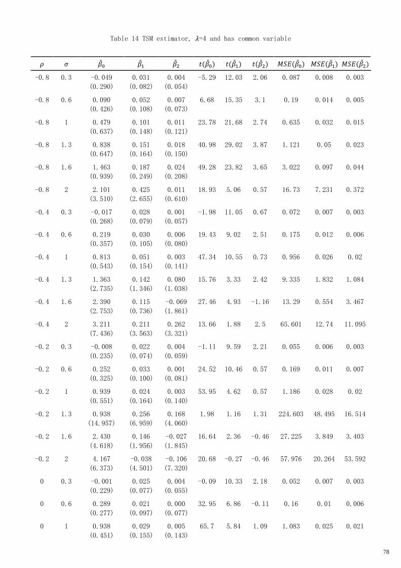
78
Table 14 TSM estimator, 𝜆=4 and has common variable
𝜌 𝜎 ��0 ��1 ��2 𝑡(��0) 𝑡(��1) 𝑡(��2) 𝑀𝑆𝐸(��0) 𝑀𝑆𝐸(��1) 𝑀𝑆𝐸(��2)
-0.8 0.3 -0.049
(0.290)
0.031
(0.082)
0.004
(0.054)
-5.29 12.03 2.06 0.087 0.008 0.003
-0.8 0.6 0.090
(0.426)
0.052
(0.108)
0.007
(0.073)
6.68 15.35 3.1 0.19 0.014 0.005
-0.8 1 0.479
(0.637)
0.101
(0.148)
0.011
(0.121)
23.78 21.68 2.74 0.635 0.032 0.015
-0.8 1.3 0.838
(0.647)
0.151
(0.164)
0.018
(0.150)
40.98 29.02 3.87 1.121 0.05 0.023
-0.8 1.6 1.463
(0.939)
0.187
(0.249)
0.024
(0.208)
49.28 23.82 3.65 3.022 0.097 0.044
-0.8 2 2.101
(3.510)
0.425
(2.655)
0.011
(0.610)
18.93 5.06 0.57 16.73 7.231 0.372
-0.4 0.3 -0.017
(0.268)
0.028
(0.079)
0.001
(0.057)
-1.98 11.05 0.67 0.072 0.007 0.003
-0.4 0.6 0.219
(0.357)
0.030
(0.105)
0.006
(0.080)
19.43 9.02 2.51 0.175 0.012 0.006
-0.4 1 0.813
(0.543)
0.051
(0.154)
0.003
(0.141)
47.34 10.55 0.73 0.956 0.026 0.02
-0.4 1.3 1.363
(2.735)
0.142
(1.346)
0.080
(1.038)
15.76 3.33 2.42 9.335 1.832 1.084
-0.4 1.6 2.390
(2.753)
0.115
(0.736)
-0.069
(1.861)
27.46 4.93 -1.16 13.29 0.554 3.467
-0.4 2 3.211
(7.436)
0.211
(3.563)
0.262
(3.321)
13.66 1.88 2.5 65.601 12.74 11.095
-0.2 0.3 -0.008
(0.235)
0.022
(0.074)
0.004
(0.059)
-1.11 9.59 2.21 0.055 0.006 0.003
-0.2 0.6 0.252
(0.325)
0.033
(0.100)
0.001
(0.081)
24.52 10.46 0.57 0.169 0.011 0.007
-0.2 1 0.939
(0.551)
0.024
(0.164)
0.003
(0.140)
53.95 4.62 0.57 1.186 0.028 0.02
-0.2 1.3 0.938
(14.957)
0.256
(6.959)
0.168
(4.060)
1.98 1.16 1.31 224.603 48.495 16.514
-0.2 1.6 2.430
(4.618)
0.146
(1.956)
-0.027
(1.845)
16.64 2.36 -0.46 27.225 3.849 3.403
-0.2 2 4.167
(6.373)
-0.038
(4.501)
-0.106
(7.320)
20.68 -0.27 -0.46 57.976 20.264 53.592
0 0.3 -0.001
(0.229)
0.025
(0.077)
0.004
(0.055)
-0.09 10.33 2.18 0.052 0.007 0.003
0 0.6 0.289
(0.277)
0.021
(0.097)
0.000
(0.077)
32.95 6.86 -0.11 0.16 0.01 0.006
0 1 0.938
(0.451)
0.029
(0.155)
0.005
(0.143)
65.7 5.84 1.09 1.083 0.025 0.021

79
𝜌 𝜎 ��0 ��1 ��2 𝑡(��0) 𝑡(��1) 𝑡(��2) 𝑀𝑆𝐸(��0) 𝑀𝑆𝐸(��1) 𝑀𝑆𝐸(��2)
0 1.3 1.587
(1.477)
0.095
(1.394)
0.014
(0.991)
33.97 2.16 0.46 4.699 1.953 0.983
0 1.6 2.582
(3.803)
0.037
(1.106)
0.042
(1.297)
21.47 1.07 1.03 21.13 1.224 1.685
0 2 3.809
(7.986)
0.249
(3.469)
-0.065
(5.920)
15.08 2.27 -0.35 78.283 12.095 35.049
0.2 0.3 0.033
(0.209)
0.015
(0.070)
-0.002
(0.055)
5.02 6.61 -1.26 0.045 0.005 0.003
0.2 0.6 0.308
(0.260)
0.019
(0.095)
-0.001
(0.079)
37.42 6.22 -0.26 0.163 0.009 0.006
0.2 1 0.966
(0.413)
0.017
(0.151)
0.016
(0.140)
73.86 3.65 3.62 1.103 0.023 0.02
0.2 1.3 1.705
(1.164)
0.034
(0.842)
0.029
(0.401)
46.3 1.28 2.27 4.261 0.709 0.162
0.2 1.6 2.619
(2.489)
0.048
(1.310)
0.076
(1.590)
33.28 1.16 1.51 13.052 1.719 2.535
0.2 2 4.272
(4.605)
0.027
(1.528)
-0.051
(6.073)
29.34 0.55 -0.27 39.458 2.337 36.889
0.4 0.3 0.036
(0.194)
0.015
(0.069)
0.002
(0.053)
5.79 7.08 1.2 0.039 0.005 0.003
0.4 0.6 0.312
(0.242)
0.016
(0.090)
0.000
(0.078)
40.86 5.74 -0.17 0.156 0.008 0.006
0.4 1 0.985
(0.443)
0.020
(0.156)
0.001
(0.183)
70.35 4.02 0.18 1.166 0.025 0.033
0.4 1.3 1.374
(14.876)
0.229
(7.101)
0.030
(1.063)
2.92 1.02 0.91 223.196 50.472 1.13
0.4 1.6 2.631
(3.426)
-0.007
(0.492)
0.101
(2.273)
24.28 -0.48 1.41 18.66 0.242 5.179
0.4 2 4.114
(7.496)
0.106
(3.133)
0.031
(2.744)
17.36 1.07 0.36 73.108 9.828 7.529
0.8 0.3 0.030
(0.181)
0.016
(0.066)
0.002
(0.054)
5.17 7.58 1.41 0.034 0.005 0.003
0.8 0.6 0.328
(0.203)
0.010
(0.083)
0.001
(0.076)
51.14 3.68 0.58 0.149 0.007 0.006
0.8 1 1.030
(0.295)
-0.002
(0.131)
0.005
(0.124)
110.4 -0.54 1.19 1.148 0.017 0.015
0.8 1.3 1.741
(2.733)
0.005
(0.521)
0.016
(1.445)
20.15 0.28 0.35 10.499 0.271 2.088
0.8 1.6 2.568
(6.387)
0.100
(3.599)
-0.035
(2.838)
12.71 0.88 -0.39 47.39 12.963 8.056
0.8 2 4.296
(7.830)
-0.020
(4.084)
0.060
(4.012)
17.35 -0.15 0.47 79.765 16.682 16.1
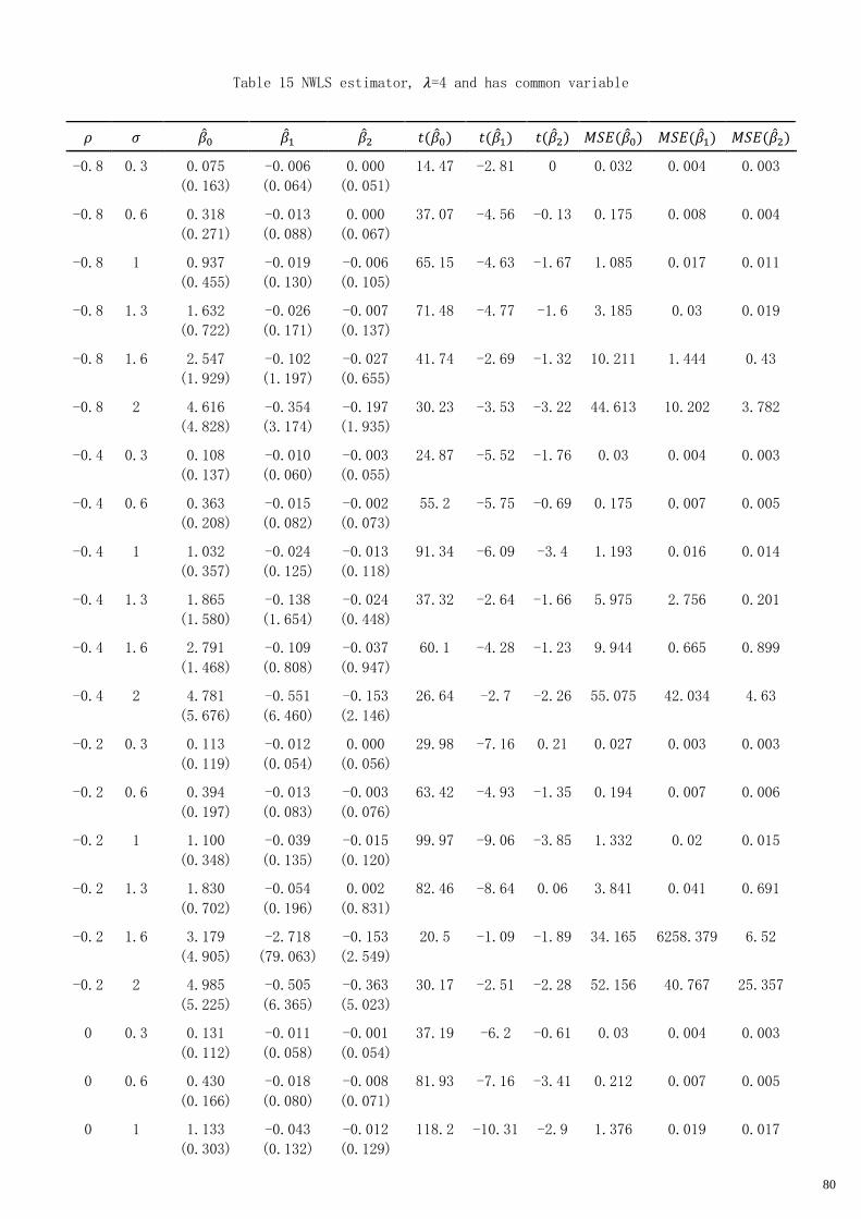
80
Table 15 NWLS estimator, 𝜆=4 and has common variable
𝜌 𝜎 ��0 ��1 ��2 𝑡(��0) 𝑡(��1) 𝑡(��2) 𝑀𝑆𝐸(��0) 𝑀𝑆𝐸(��1) 𝑀𝑆𝐸(��2)
-0.8 0.3 0.075
(0.163)
-0.006
(0.064)
0.000
(0.051)
14.47 -2.81 0 0.032 0.004 0.003
-0.8 0.6 0.318
(0.271)
-0.013
(0.088)
0.000
(0.067)
37.07 -4.56 -0.13 0.175 0.008 0.004
-0.8 1 0.937
(0.455)
-0.019
(0.130)
-0.006
(0.105)
65.15 -4.63 -1.67 1.085 0.017 0.011
-0.8 1.3 1.632
(0.722)
-0.026
(0.171)
-0.007
(0.137)
71.48 -4.77 -1.6 3.185 0.03 0.019
-0.8 1.6 2.547
(1.929)
-0.102
(1.197)
-0.027
(0.655)
41.74 -2.69 -1.32 10.211 1.444 0.43
-0.8 2 4.616
(4.828)
-0.354
(3.174)
-0.197
(1.935)
30.23 -3.53 -3.22 44.613 10.202 3.782
-0.4 0.3 0.108
(0.137)
-0.010
(0.060)
-0.003
(0.055)
24.87 -5.52 -1.76 0.03 0.004 0.003
-0.4 0.6 0.363
(0.208)
-0.015
(0.082)
-0.002
(0.073)
55.2 -5.75 -0.69 0.175 0.007 0.005
-0.4 1 1.032
(0.357)
-0.024
(0.125)
-0.013
(0.118)
91.34 -6.09 -3.4 1.193 0.016 0.014
-0.4 1.3 1.865
(1.580)
-0.138
(1.654)
-0.024
(0.448)
37.32 -2.64 -1.66 5.975 2.756 0.201
-0.4 1.6 2.791
(1.468)
-0.109
(0.808)
-0.037
(0.947)
60.1 -4.28 -1.23 9.944 0.665 0.899
-0.4 2 4.781
(5.676)
-0.551
(6.460)
-0.153
(2.146)
26.64 -2.7 -2.26 55.075 42.034 4.63
-0.2 0.3 0.113
(0.119)
-0.012
(0.054)
0.000
(0.056)
29.98 -7.16 0.21 0.027 0.003 0.003
-0.2 0.6 0.394
(0.197)
-0.013
(0.083)
-0.003
(0.076)
63.42 -4.93 -1.35 0.194 0.007 0.006
-0.2 1 1.100
(0.348)
-0.039
(0.135)
-0.015
(0.120)
99.97 -9.06 -3.85 1.332 0.02 0.015
-0.2 1.3 1.830
(0.702)
-0.054
(0.196)
0.002
(0.831)
82.46 -8.64 0.06 3.841 0.041 0.691
-0.2 1.6 3.179
(4.905)
-2.718
(79.063)
-0.153
(2.549)
20.5 -1.09 -1.89 34.165 6258.379 6.52
-0.2 2 4.985
(5.225)
-0.505
(6.365)
-0.363
(5.023)
30.17 -2.51 -2.28 52.156 40.767 25.357
0 0.3 0.131
(0.112)
-0.011
(0.058)
-0.001
(0.054)
37.19 -6.2 -0.61 0.03 0.004 0.003
0 0.6 0.430
(0.166)
-0.018
(0.080)
-0.008
(0.071)
81.93 -7.16 -3.41 0.212 0.007 0.005
0 1 1.133
(0.303)
-0.043
(0.132)
-0.012
(0.129)
118.2 -10.31 -2.9 1.376 0.019 0.017
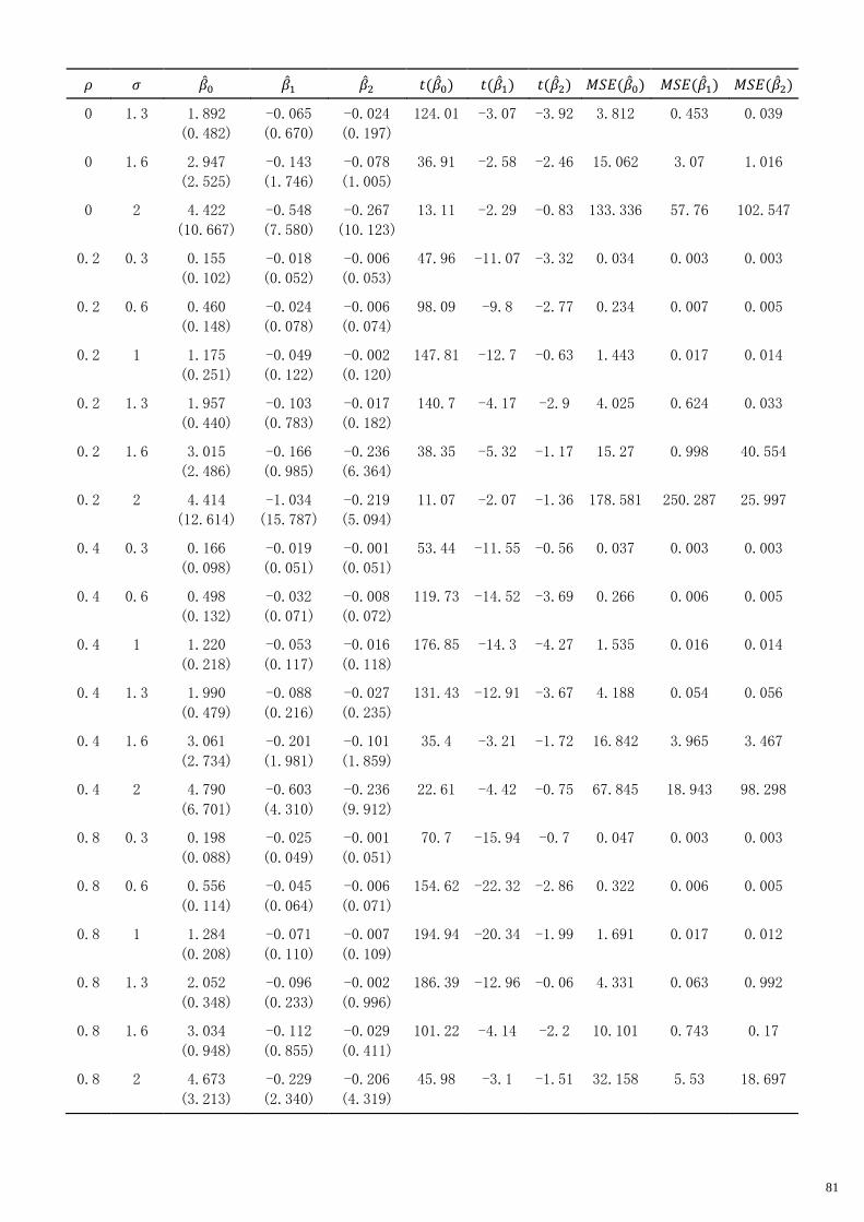
81
𝜌 𝜎 ��0 ��1 ��2 𝑡(��0) 𝑡(��1) 𝑡(��2) 𝑀𝑆𝐸(��0) 𝑀𝑆𝐸(��1) 𝑀𝑆𝐸(��2)
0 1.3 1.892
(0.482)
-0.065
(0.670)
-0.024
(0.197)
124.01 -3.07 -3.92 3.812 0.453 0.039
0 1.6 2.947
(2.525)
-0.143
(1.746)
-0.078
(1.005)
36.91 -2.58 -2.46 15.062 3.07 1.016
0 2 4.422
(10.667)
-0.548
(7.580)
-0.267
(10.123)
13.11 -2.29 -0.83 133.336 57.76 102.547
0.2 0.3 0.155
(0.102)
-0.018
(0.052)
-0.006
(0.053)
47.96 -11.07 -3.32 0.034 0.003 0.003
0.2 0.6 0.460
(0.148)
-0.024
(0.078)
-0.006
(0.074)
98.09 -9.8 -2.77 0.234 0.007 0.005
0.2 1 1.175
(0.251)
-0.049
(0.122)
-0.002
(0.120)
147.81 -12.7 -0.63 1.443 0.017 0.014
0.2 1.3 1.957
(0.440)
-0.103
(0.783)
-0.017
(0.182)
140.7 -4.17 -2.9 4.025 0.624 0.033
0.2 1.6 3.015
(2.486)
-0.166
(0.985)
-0.236
(6.364)
38.35 -5.32 -1.17 15.27 0.998 40.554
0.2 2 4.414
(12.614)
-1.034
(15.787)
-0.219
(5.094)
11.07 -2.07 -1.36 178.581 250.287 25.997
0.4 0.3 0.166
(0.098)
-0.019
(0.051)
-0.001
(0.051)
53.44 -11.55 -0.56 0.037 0.003 0.003
0.4 0.6 0.498
(0.132)
-0.032
(0.071)
-0.008
(0.072)
119.73 -14.52 -3.69 0.266 0.006 0.005
0.4 1 1.220
(0.218)
-0.053
(0.117)
-0.016
(0.118)
176.85 -14.3 -4.27 1.535 0.016 0.014
0.4 1.3 1.990
(0.479)
-0.088
(0.216)
-0.027
(0.235)
131.43 -12.91 -3.67 4.188 0.054 0.056
0.4 1.6 3.061
(2.734)
-0.201
(1.981)
-0.101
(1.859)
35.4 -3.21 -1.72 16.842 3.965 3.467
0.4 2 4.790
(6.701)
-0.603
(4.310)
-0.236
(9.912)
22.61 -4.42 -0.75 67.845 18.943 98.298
0.8 0.3 0.198
(0.088)
-0.025
(0.049)
-0.001
(0.051)
70.7 -15.94 -0.7 0.047 0.003 0.003
0.8 0.6 0.556
(0.114)
-0.045
(0.064)
-0.006
(0.071)
154.62 -22.32 -2.86 0.322 0.006 0.005
0.8 1 1.284
(0.208)
-0.071
(0.110)
-0.007
(0.109)
194.94 -20.34 -1.99 1.691 0.017 0.012
0.8 1.3 2.052
(0.348)
-0.096
(0.233)
-0.002
(0.996)
186.39 -12.96 -0.06 4.331 0.063 0.992
0.8 1.6 3.034
(0.948)
-0.112
(0.855)
-0.029
(0.411)
101.22 -4.14 -2.2 10.101 0.743 0.17
0.8 2 4.673
(3.213)
-0.229
(2.340)
-0.206
(4.319)
45.98 -3.1 -1.51 32.158 5.53 18.697
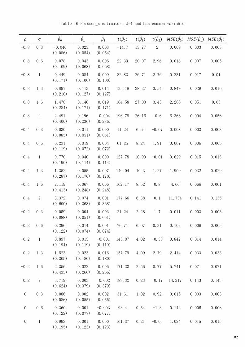
82
Table 16 Poisson_s estimator, 𝜆=4 and has common variable
𝜌 𝜎 ��0 ��1 ��2 𝑡(��0) 𝑡(��1) 𝑡(��2) 𝑀𝑆𝐸(��0) 𝑀𝑆𝐸(��1) 𝑀𝑆𝐸(��2)
-0.8 0.3 -0.040
(0.086)
0.023
(0.054)
0.003
(0.054)
-14.7 13.77 2 0.009 0.003 0.003
-0.8 0.6 0.078
(0.109)
0.043
(0.068)
0.006
(0.068)
22.39 20.07 2.96 0.018 0.007 0.005
-0.8 1 0.449
(0.171)
0.084
(0.100)
0.009
(0.100)
82.83 26.71 2.76 0.231 0.017 0.01
-0.8 1.3 0.897
(0.210)
0.113
(0.127)
0.014
(0.127)
135.18 28.27 3.54 0.849 0.029 0.016
-0.8 1.6 1.478
(0.284)
0.146
(0.171)
0.019
(0.171)
164.58 27.03 3.45 2.265 0.051 0.03
-0.8 2 2.491
(0.400)
0.196
(0.236)
-0.004
(0.236)
196.78 26.16 -0.6 6.366 0.094 0.056
-0.4 0.3 0.030
(0.085)
0.011
(0.051)
0.000
(0.051)
11.24 6.64 -0.07 0.008 0.003 0.003
-0.4 0.6 0.231
(0.119)
0.019
(0.072)
0.004
(0.072)
61.25 8.24 1.91 0.067 0.006 0.005
-0.4 1 0.770
(0.190)
0.040
(0.114)
0.000
(0.114)
127.78 10.99 -0.01 0.629 0.015 0.013
-0.4 1.3 1.352
(0.287)
0.055
(0.170)
0.007
(0.170)
149.04 10.3 1.27 1.909 0.032 0.029
-0.4 1.6 2.119
(0.413)
0.067
(0.248)
0.006
(0.248)
162.17 8.52 0.8 4.66 0.066 0.061
-0.4 2 3.372
(0.600)
0.074
(0.368)
0.001
(0.368)
177.66 6.38 0.1 11.734 0.141 0.135
-0.2 0.3 0.059
(0.088)
0.004
(0.051)
0.003
(0.051)
21.24 2.28 1.7 0.011 0.003 0.003
-0.2 0.6 0.296
(0.122)
0.014
(0.074)
0.001
(0.074)
76.71 6.07 0.31 0.102 0.006 0.005
-0.2 1 0.897
(0.194)
0.015
(0.119)
-0.001
(0.119)
145.87 4.02 -0.38 0.842 0.014 0.014
-0.2 1.3 1.523
(0.305)
0.023
(0.180)
0.016
(0.180)
157.79 4.09 2.79 2.414 0.033 0.033
-0.2 1.6 2.356
(0.435)
0.022
(0.266)
0.006
(0.266)
171.23 2.56 0.77 5.741 0.071 0.071
-0.2 2 3.719
(0.624)
0.003
(0.379)
-0.002
(0.379)
188.32 0.23 -0.17 14.217 0.143 0.143
0 0.3 0.086
(0.086)
0.002
(0.055)
0.002
(0.055)
31.61 1.02 0.92 0.015 0.003 0.003
0 0.6 0.360
(0.122)
0.001
(0.077)
-0.003
(0.077)
93.4 0.54 -1.3 0.144 0.006 0.006
0 1 0.993
(0.195)
0.001
(0.123)
0.000
(0.123)
161.37 0.21 -0.05 1.024 0.015 0.015
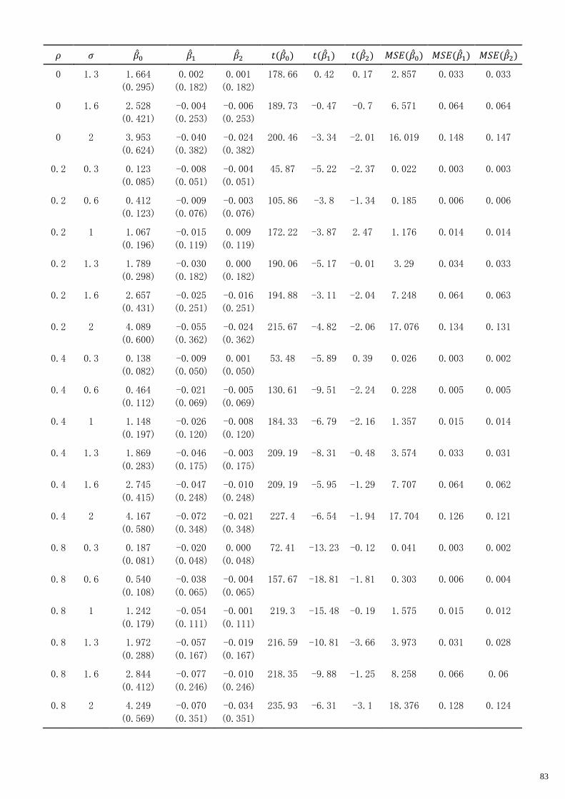
83
𝜌 𝜎 ��0 ��1 ��2 𝑡(��0) 𝑡(��1) 𝑡(��2) 𝑀𝑆𝐸(��0) 𝑀𝑆𝐸(��1) 𝑀𝑆𝐸(��2)
0 1.3 1.664
(0.295)
0.002
(0.182)
0.001
(0.182)
178.66 0.42 0.17 2.857 0.033 0.033
0 1.6 2.528
(0.421)
-0.004
(0.253)
-0.006
(0.253)
189.73 -0.47 -0.7 6.571 0.064 0.064
0 2 3.953
(0.624)
-0.040
(0.382)
-0.024
(0.382)
200.46 -3.34 -2.01 16.019 0.148 0.147
0.2 0.3 0.123
(0.085)
-0.008
(0.051)
-0.004
(0.051)
45.87 -5.22 -2.37 0.022 0.003 0.003
0.2 0.6 0.412
(0.123)
-0.009
(0.076)
-0.003
(0.076)
105.86 -3.8 -1.34 0.185 0.006 0.006
0.2 1 1.067
(0.196)
-0.015
(0.119)
0.009
(0.119)
172.22 -3.87 2.47 1.176 0.014 0.014
0.2 1.3 1.789
(0.298)
-0.030
(0.182)
0.000
(0.182)
190.06 -5.17 -0.01 3.29 0.034 0.033
0.2 1.6 2.657
(0.431)
-0.025
(0.251)
-0.016
(0.251)
194.88 -3.11 -2.04 7.248 0.064 0.063
0.2 2 4.089
(0.600)
-0.055
(0.362)
-0.024
(0.362)
215.67 -4.82 -2.06 17.076 0.134 0.131
0.4 0.3 0.138
(0.082)
-0.009
(0.050)
0.001
(0.050)
53.48 -5.89 0.39 0.026 0.003 0.002
0.4 0.6 0.464
(0.112)
-0.021
(0.069)
-0.005
(0.069)
130.61 -9.51 -2.24 0.228 0.005 0.005
0.4 1 1.148
(0.197)
-0.026
(0.120)
-0.008
(0.120)
184.33 -6.79 -2.16 1.357 0.015 0.014
0.4 1.3 1.869
(0.283)
-0.046
(0.175)
-0.003
(0.175)
209.19 -8.31 -0.48 3.574 0.033 0.031
0.4 1.6 2.745
(0.415)
-0.047
(0.248)
-0.010
(0.248)
209.19 -5.95 -1.29 7.707 0.064 0.062
0.4 2 4.167
(0.580)
-0.072
(0.348)
-0.021
(0.348)
227.4 -6.54 -1.94 17.704 0.126 0.121
0.8 0.3 0.187
(0.081)
-0.020
(0.048)
0.000
(0.048)
72.41 -13.23 -0.12 0.041 0.003 0.002
0.8 0.6 0.540
(0.108)
-0.038
(0.065)
-0.004
(0.065)
157.67 -18.81 -1.81 0.303 0.006 0.004
0.8 1 1.242
(0.179)
-0.054
(0.111)
-0.001
(0.111)
219.3 -15.48 -0.19 1.575 0.015 0.012
0.8 1.3 1.972
(0.288)
-0.057
(0.167)
-0.019
(0.167)
216.59 -10.81 -3.66 3.973 0.031 0.028
0.8 1.6 2.844
(0.412)
-0.077
(0.246)
-0.010
(0.246)
218.35 -9.88 -1.25 8.258 0.066 0.06
0.8 2 4.249
(0.569)
-0.070
(0.351)
-0.034
(0.351)
235.93 -6.31 -3.1 18.376 0.128 0.124

84
Table 17 Poisson_f estimator, 𝜆=4 and has common variable
𝜌 𝜎 ��0 ��1 ��2 𝑡(��0) 𝑡(��1) 𝑡(��2) 𝑀𝑆𝐸(��0) 𝑀𝑆𝐸(��1) 𝑀𝑆𝐸(��2)
-0.8 0.3 0.086
(0.077)
0.002
(0.047)
0.001
(0.077)
35.47 1.21 0.25 0.013 0.002 0.006
-0.8 0.6 0.361
(0.107)
-0.002
(0.064)
0.000
(0.107)
106.67 -1.2 0.09 0.141 0.004 0.011
-0.8 1 1.003
(0.178)
-0.003
(0.108)
-0.001
(0.178)
177.95 -0.9 -0.11 1.037 0.012 0.032
-0.8 1.3 1.682
(0.260)
-0.005
(0.169)
-0.003
(0.260)
204.76 -1.01 -0.38 2.896 0.029 0.067
-0.8 1.6 2.549
(0.400)
-0.009
(0.234)
-0.010
(0.400)
201.72 -1.27 -0.79 6.656 0.055 0.16
-0.8 2 3.947
(0.571)
-0.018
(0.337)
-0.031
(0.571)
218.57 -1.64 -1.73 15.909 0.114 0.327
-0.4 0.3 0.091
(0.072)
-0.001
(0.043)
0.000
(0.072)
39.8 -0.78 -0.22 0.013 0.002 0.005
-0.4 0.6 0.357
(0.105)
-0.001
(0.065)
0.001
(0.105)
107.3 -0.6 0.37 0.138 0.004 0.011
-0.4 1 0.998
(0.175)
-0.001
(0.105)
-0.005
(0.175)
179.98 -0.39 -0.86 1.027 0.011 0.031
-0.4 1.3 1.670
(0.273)
-0.001
(0.159)
0.003
(0.273)
193.24 -0.1 0.32 2.864 0.025 0.075
-0.4 1.6 2.544
(0.378)
-0.004
(0.238)
-0.010
(0.378)
212.87 -0.56 -0.82 6.612 0.057 0.143
-0.4 2 3.928
(0.566)
-0.023
(0.360)
-0.014
(0.566)
219.35 -2.02 -0.78 15.75 0.13 0.321
-0.2 0.3 0.088
(0.076)
0.000
(0.045)
0.001
(0.076)
36.54 0.18 0.34 0.014 0.002 0.006
-0.2 0.6 0.355
(0.105)
0.003
(0.064)
0.001
(0.105)
106.86 1.68 0.21 0.137 0.004 0.011
-0.2 1 1.002
(0.168)
-0.004
(0.104)
-0.001
(0.168)
188.18 -1.2 -0.25 1.032 0.011 0.028
-0.2 1.3 1.673
(0.261)
-0.005
(0.160)
0.012
(0.261)
202.47 -1.03 1.46 2.869 0.026 0.068
-0.2 1.6 2.536
(0.390)
-0.008
(0.242)
0.001
(0.390)
205.47 -1.05 0.11 6.583 0.059 0.152
-0.2 2 3.962
(0.584)
-0.031
(0.346)
-0.017
(0.584)
214.54 -2.86 -0.92 16.038 0.121 0.341
0 0.3 0.086
(0.075)
0.002
(0.047)
0.002
(0.075)
36.47 1.59 0.7 0.013 0.002 0.006
0 0.6 0.359
(0.107)
0.000
(0.067)
-0.002
(0.107)
105.84 0.19 -0.48 0.14 0.004 0.011
0 1 0.992
(0.174)
0.001
(0.111)
0.003
(0.174)
179.82 0.2 0.57 1.014 0.012 0.03

85
𝜌 𝜎 ��0 ��1 ��2 𝑡(��0) 𝑡(��1) 𝑡(��2) 𝑀𝑆𝐸(��0) 𝑀𝑆𝐸(��1) 𝑀𝑆𝐸(��2)
0 1.3 1.679
(0.253)
-0.002
(0.158)
-0.002
(0.253)
209.8 -0.45 -0.24 2.882 0.025 0.064
0 1.6 2.539
(0.382)
-0.005
(0.236)
-0.003
(0.382)
209.94 -0.72 -0.23 6.591 0.056 0.146
0 2 3.965
(0.553)
-0.032
(0.337)
-0.023
(0.553)
226.58 -3.03 -1.29 16.03 0.114 0.307
0.2 0.3 0.093
(0.075)
-0.002
(0.044)
-0.002
(0.075)
39.21 -1.39 -0.75 0.014 0.002 0.006
0.2 0.6 0.358
(0.109)
0.001
(0.067)
-0.002
(0.109)
104.25 0.58 -0.44 0.14 0.004 0.012
0.2 1 0.986
(0.175)
-0.002
(0.109)
0.011
(0.175)
178.68 -0.47 2 1.004 0.012 0.031
0.2 1.3 1.687
(0.269)
-0.009
(0.164)
0.000
(0.269)
198.1 -1.64 -0.01 2.919 0.027 0.073
0.2 1.6 2.538
(0.390)
0.001
(0.225)
-0.017
(0.390)
205.82 0.12 -1.4 6.594 0.051 0.152
0.2 2 3.958
(0.560)
-0.029
(0.334)
-0.021
(0.560)
223.37 -2.74 -1.21 15.979 0.113 0.314
0.4 0.3 0.085
(0.073)
0.001
(0.045)
0.002
(0.073)
36.69 0.35 1 0.013 0.002 0.005
0.4 0.6 0.360
(0.103)
0.000
(0.064)
-0.001
(0.103)
110.49 -0.12 -0.32 0.14 0.004 0.011
0.4 1 0.996
(0.179)
0.003
(0.109)
-0.004
(0.179)
176.33 0.93 -0.66 1.024 0.012 0.032
0.4 1.3 1.688
(0.260)
-0.009
(0.162)
0.000
(0.260)
205.18 -1.77 -0.03 2.916 0.026 0.068
0.4 1.6 2.535
(0.381)
-0.003
(0.230)
-0.005
(0.381)
210.36 -0.38 -0.46 6.573 0.053 0.145
0.4 2 3.933
(0.546)
-0.023
(0.328)
-0.015
(0.546)
227.61 -2.2 -0.88 15.763 0.108 0.299
0.8 0.3 0.086
(0.077)
0.000
(0.045)
0.002
(0.077)
35.2 -0.05 0.79 0.013 0.002 0.006
0.8 0.6 0.364
(0.104)
-0.004
(0.063)
0.000
(0.104)
110.5 -1.94 0.07 0.144 0.004 0.011
0.8 1 0.999
(0.174)
-0.005
(0.109)
0.003
(0.174)
182.08 -1.36 0.56 1.029 0.012 0.03
0.8 1.3 1.692
(0.279)
0.002
(0.162)
-0.013
(0.279)
191.65 0.3 -1.43 2.942 0.026 0.078
0.8 1.6 2.541
(0.405)
-0.010
(0.241)
-0.005
(0.405)
198.28 -1.34 -0.39 6.623 0.058 0.164
0.8 2 3.927
(0.562)
0.001
(0.348)
-0.026
(0.562)
221.11 0.11 -1.44 15.739 0.121 0.316

86
Table 18 FIML estimator, 𝜆=4 and does not have common variable
𝜌 𝜎 ��0 ��1 ��2 𝑡(��0) 𝑡(��1) 𝑡(��2) 𝑀𝑆𝐸(��0) 𝑀𝑆𝐸(��1) 𝑀𝑆𝐸(��2)
-0.8 0.3 0.030
(0.098)
-0.003
(0.050)
0.002
(0.050)
9.82 -2.02 1.21 0.01 0.003 0.003
-0.8 0.6 0.123
(0.135)
-0.005
(0.068)
0.006
(0.067)
28.86 -2.5 3.03 0.033 0.005 0.005
-0.8 1 0.381
(0.203)
-0.010
(0.119)
0.007
(0.122)
59.34 -2.55 1.81 0.186 0.014 0.015
-0.8 1.3 0.772
(0.308)
-0.016
(0.190)
-0.001
(0.191)
79.35 -2.73 -0.19 0.691 0.036 0.037
-0.8 1.6 1.305
(0.444)
-0.036
(0.306)
-0.014
(0.301)
93 -3.75 -1.48 1.899 0.095 0.091
-0.8 2 2.190
(0.683)
-0.077
(0.457)
-0.035
(0.438)
101.44 -5.32 -2.55 5.26 0.215 0.193
-0.4 0.3 0.079
(0.113)
0.001
(0.052)
0.002
(0.052)
22.01 0.45 1.14 0.019 0.003 0.003
-0.4 0.6 0.196
(0.153)
-0.002
(0.082)
0.002
(0.081)
40.32 -0.72 0.59 0.062 0.007 0.007
-0.4 1 0.622
(0.295)
0.005
(0.188)
-0.002
(0.197)
66.64 0.86 -0.33 0.474 0.035 0.039
-0.4 1.3 1.141
(0.494)
0.004
(0.334)
0.005
(0.332)
73.05 0.34 0.46 1.547 0.111 0.11
-0.4 1.6 1.798
(0.733)
-0.052
(0.509)
0.004
(0.499)
77.59 -3.2 0.27 3.77 0.262 0.249
-0.4 2 2.838
(1.080)
-0.145
(0.731)
-0.063
(0.747)
83.12 -6.27 -2.65 9.222 0.555 0.562
-0.2 0.3 0.103
(0.115)
0.002
(0.052)
0.001
(0.052)
28.28 1.28 0.84 0.024 0.003 0.003
-0.2 0.6 0.232
(0.150)
0.000
(0.080)
0.000
(0.080)
48.88 0.11 0.13 0.077 0.006 0.006
-0.2 1 0.713
(0.318)
0.004
(0.217)
0.005
(0.218)
71.03 0.64 0.78 0.609 0.047 0.048
-0.2 1.3 1.308
(0.515)
-0.001
(0.368)
-0.005
(0.358)
80.33 -0.1 -0.45 1.976 0.136 0.128
-0.2 1.6 1.960
(0.789)
-0.036
(0.552)
0.030
(0.537)
78.54 -2.05 1.76 4.466 0.306 0.289
-0.2 2 3.017
(1.102)
-0.139
(0.783)
-0.015
(0.757)
86.57 -5.59 -0.64 10.314 0.632 0.573
0 0.3 0.127
(0.119)
-0.003
(0.051)
-0.001
(0.049)
33.69 -1.79 -0.74 0.03 0.003 0.002
0 0.6 0.277
(0.142)
0.006
(0.083)
-0.007
(0.080)
61.74 2.48 -2.71 0.097 0.007 0.006
0 1 0.807
(0.322)
0.006
(0.221)
0.002
(0.232)
79.28 0.79 0.21 0.755 0.049 0.054
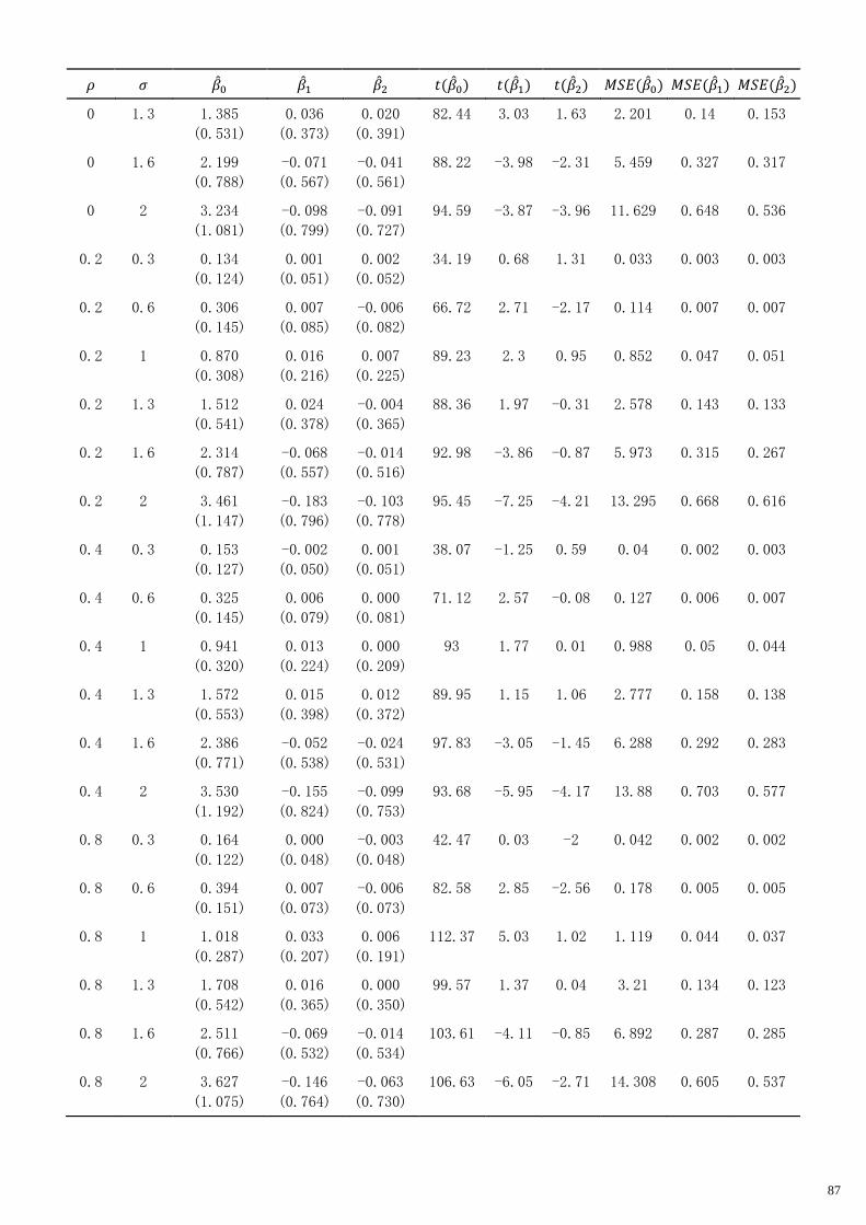
87
𝜌 𝜎 ��0 ��1 ��2 𝑡(��0) 𝑡(��1) 𝑡(��2) 𝑀𝑆𝐸(��0) 𝑀𝑆𝐸(��1) 𝑀𝑆𝐸(��2)
0 1.3 1.385
(0.531)
0.036
(0.373)
0.020
(0.391)
82.44 3.03 1.63 2.201 0.14 0.153
0 1.6 2.199
(0.788)
-0.071
(0.567)
-0.041
(0.561)
88.22 -3.98 -2.31 5.459 0.327 0.317
0 2 3.234
(1.081)
-0.098
(0.799)
-0.091
(0.727)
94.59 -3.87 -3.96 11.629 0.648 0.536
0.2 0.3 0.134
(0.124)
0.001
(0.051)
0.002
(0.052)
34.19 0.68 1.31 0.033 0.003 0.003
0.2 0.6 0.306
(0.145)
0.007
(0.085)
-0.006
(0.082)
66.72 2.71 -2.17 0.114 0.007 0.007
0.2 1 0.870
(0.308)
0.016
(0.216)
0.007
(0.225)
89.23 2.3 0.95 0.852 0.047 0.051
0.2 1.3 1.512
(0.541)
0.024
(0.378)
-0.004
(0.365)
88.36 1.97 -0.31 2.578 0.143 0.133
0.2 1.6 2.314
(0.787)
-0.068
(0.557)
-0.014
(0.516)
92.98 -3.86 -0.87 5.973 0.315 0.267
0.2 2 3.461
(1.147)
-0.183
(0.796)
-0.103
(0.778)
95.45 -7.25 -4.21 13.295 0.668 0.616
0.4 0.3 0.153
(0.127)
-0.002
(0.050)
0.001
(0.051)
38.07 -1.25 0.59 0.04 0.002 0.003
0.4 0.6 0.325
(0.145)
0.006
(0.079)
0.000
(0.081)
71.12 2.57 -0.08 0.127 0.006 0.007
0.4 1 0.941
(0.320)
0.013
(0.224)
0.000
(0.209)
93 1.77 0.01 0.988 0.05 0.044
0.4 1.3 1.572
(0.553)
0.015
(0.398)
0.012
(0.372)
89.95 1.15 1.06 2.777 0.158 0.138
0.4 1.6 2.386
(0.771)
-0.052
(0.538)
-0.024
(0.531)
97.83 -3.05 -1.45 6.288 0.292 0.283
0.4 2 3.530
(1.192)
-0.155
(0.824)
-0.099
(0.753)
93.68 -5.95 -4.17 13.88 0.703 0.577
0.8 0.3 0.164
(0.122)
0.000
(0.048)
-0.003
(0.048)
42.47 0.03 -2 0.042 0.002 0.002
0.8 0.6 0.394
(0.151)
0.007
(0.073)
-0.006
(0.073)
82.58 2.85 -2.56 0.178 0.005 0.005
0.8 1 1.018
(0.287)
0.033
(0.207)
0.006
(0.191)
112.37 5.03 1.02 1.119 0.044 0.037
0.8 1.3 1.708
(0.542)
0.016
(0.365)
0.000
(0.350)
99.57 1.37 0.04 3.21 0.134 0.123
0.8 1.6 2.511
(0.766)
-0.069
(0.532)
-0.014
(0.534)
103.61 -4.11 -0.85 6.892 0.287 0.285
0.8 2 3.627
(1.075)
-0.146
(0.764)
-0.063
(0.730)
106.63 -6.05 -2.71 14.308 0.605 0.537
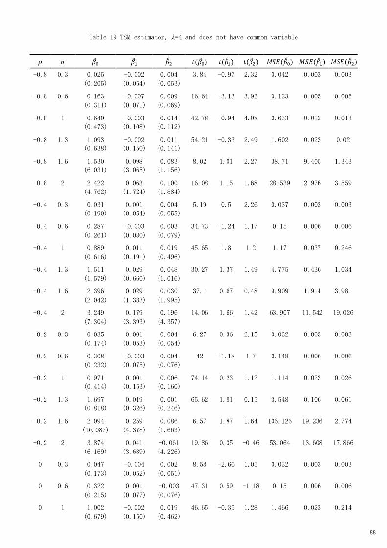
88
Table 19 TSM estimator, 𝜆=4 and does not have common variable
𝜌 𝜎 ��0 ��1 ��2 𝑡(��0) 𝑡(��1) 𝑡(��2) 𝑀𝑆𝐸(��0) 𝑀𝑆𝐸(��1) 𝑀𝑆𝐸(��2)
-0.8 0.3 0.025
(0.205)
-0.002
(0.054)
0.004
(0.053)
3.84 -0.97 2.32 0.042 0.003 0.003
-0.8 0.6 0.163
(0.311)
-0.007
(0.071)
0.009
(0.069)
16.64 -3.13 3.92 0.123 0.005 0.005
-0.8 1 0.640
(0.473)
-0.003
(0.108)
0.014
(0.112)
42.78 -0.94 4.08 0.633 0.012 0.013
-0.8 1.3 1.093
(0.638)
-0.002
(0.150)
0.011
(0.141)
54.21 -0.33 2.49 1.602 0.023 0.02
-0.8 1.6 1.530
(6.031)
0.098
(3.065)
0.083
(1.156)
8.02 1.01 2.27 38.71 9.405 1.343
-0.8 2 2.422
(4.762)
0.063
(1.724)
0.100
(1.884)
16.08 1.15 1.68 28.539 2.976 3.559
-0.4 0.3 0.031
(0.190)
0.001
(0.054)
0.004
(0.055)
5.19 0.5 2.26 0.037 0.003 0.003
-0.4 0.6 0.287
(0.261)
-0.003
(0.080)
0.003
(0.079)
34.73 -1.24 1.17 0.15 0.006 0.006
-0.4 1 0.889
(0.616)
0.011
(0.191)
0.019
(0.496)
45.65 1.8 1.2 1.17 0.037 0.246
-0.4 1.3 1.511
(1.579)
0.029
(0.660)
0.048
(1.016)
30.27 1.37 1.49 4.775 0.436 1.034
-0.4 1.6 2.396
(2.042)
0.029
(1.383)
0.030
(1.995)
37.1 0.67 0.48 9.909 1.914 3.981
-0.4 2 3.249
(7.304)
0.179
(3.393)
0.196
(4.357)
14.06 1.66 1.42 63.907 11.542 19.026
-0.2 0.3 0.035
(0.174)
0.001
(0.053)
0.004
(0.054)
6.27 0.36 2.15 0.032 0.003 0.003
-0.2 0.6 0.308
(0.232)
-0.003
(0.075)
0.004
(0.076)
42 -1.18 1.7 0.148 0.006 0.006
-0.2 1 0.971
(0.414)
0.001
(0.153)
0.006
(0.160)
74.14 0.23 1.12 1.114 0.023 0.026
-0.2 1.3 1.697
(0.818)
0.019
(0.326)
0.001
(0.246)
65.62 1.81 0.15 3.548 0.106 0.061
-0.2 1.6 2.094
(10.087)
0.259
(4.378)
0.086
(1.663)
6.57 1.87 1.64 106.126 19.236 2.774
-0.2 2 3.874
(6.169)
0.041
(3.689)
-0.061
(4.226)
19.86 0.35 -0.46 53.064 13.608 17.866
0 0.3 0.047
(0.173)
-0.004
(0.052)
0.002
(0.051)
8.58 -2.66 1.05 0.032 0.003 0.003
0 0.6 0.322
(0.215)
0.001
(0.077)
-0.003
(0.076)
47.31 0.59 -1.18 0.15 0.006 0.006
0 1 1.002
(0.679)
-0.002
(0.150)
0.019
(0.462)
46.65 -0.35 1.28 1.466 0.023 0.214

89
𝜌 𝜎 ��0 ��1 ��2 𝑡(��0) 𝑡(��1) 𝑡(��2) 𝑀𝑆𝐸(��0) 𝑀𝑆𝐸(��1) 𝑀𝑆𝐸(��2)
0 1.3 1.691
(2.061)
0.066
(1.359)
0.028
(0.455)
25.94 1.54 1.96 7.108 1.852 0.208
0 1.6 2.610
(3.236)
0.103
(1.789)
0.039
(1.045)
25.5 1.82 1.17 17.281 3.212 1.094
0 2 3.759
(8.015)
-0.094
(6.837)
0.189
(3.675)
14.83 -0.44 1.63 78.366 46.752 13.541
0.2 0.3 0.043
(0.159)
-0.001
(0.054)
0.005
(0.054)
8.59 -0.35 2.91 0.027 0.003 0.003
0.2 0.6 0.324
(0.211)
0.004
(0.079)
-0.001
(0.078)
48.54 1.4 -0.53 0.149 0.006 0.006
0.2 1 0.990
(0.411)
0.004
(0.315)
0.015
(0.317)
76.2 0.41 1.49 1.149 0.099 0.1
0.2 1.3 1.693
(0.973)
0.025
(0.322)
0.025
(0.958)
55.02 2.47 0.83 3.815 0.104 0.919
0.2 1.6 1.975
(19.135)
0.351
(10.427)
0.183
(2.783)
3.26 1.06 2.08 370.047 108.838 7.776
0.2 2 3.933
(10.861)
-0.094
(4.255)
0.253
(5.846)
11.45 -0.7 1.37 133.422 18.112 34.238
0.4 0.3 0.054
(0.158)
-0.004
(0.052)
0.004
(0.053)
10.9 -2.39 2.15 0.028 0.003 0.003
0.4 0.6 0.317
(0.192)
0.004
(0.076)
0.004
(0.077)
52.34 1.74 1.78 0.137 0.006 0.006
0.4 1 1.012
(0.331)
0.004
(0.148)
0.004
(0.151)
96.68 0.95 0.79 1.134 0.022 0.023
0.4 1.3 1.733
(2.749)
0.025
(1.545)
0.034
(0.855)
19.93 0.51 1.26 10.559 2.386 0.732
0.4 1.6 2.657
(3.622)
0.202
(3.544)
-0.072
(2.641)
23.19 1.8 -0.87 20.179 12.602 6.981
0.4 2 4.223
(5.626)
0.097
(3.929)
0.039
(1.788)
23.74 0.78 0.69 49.487 15.448 3.198
0.8 0.3 0.050
(0.143)
-0.002
(0.050)
0.001
(0.050)
11.09 -1.45 0.81 0.023 0.002 0.002
0.8 0.6 0.345
(0.166)
0.002
(0.071)
-0.001
(0.072)
65.67 0.86 -0.43 0.147 0.005 0.005
0.8 1 1.022
(0.295)
0.007
(0.124)
0.002
(0.127)
109.47 1.72 0.44 1.132 0.015 0.016
0.8 1.3 1.765
(0.562)
0.016
(0.213)
0.008
(0.193)
99.41 2.44 1.24 3.432 0.046 0.037
0.8 1.6 2.357
(5.646)
0.162
(3.611)
0.064
(2.038)
13.2 1.42 0.99 37.428 13.068 4.157
0.8 2 3.969
(8.141)
0.235
(3.715)
-0.177
(6.294)
15.42 2 -0.89 82.033 13.855 39.647
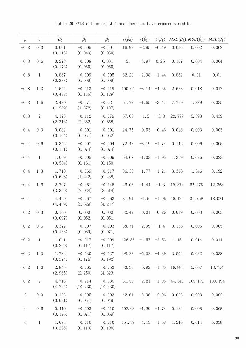
90
Table 20 NWLS estimator, 𝜆=4 and does not have common variable
𝜌 𝜎 ��0 ��1 ��2 𝑡(��0) 𝑡(��1) 𝑡(��2) 𝑀𝑆𝐸(��0) 𝑀𝑆𝐸(��1) 𝑀𝑆𝐸(��2)
-0.8 0.3 0.061
(0.113)
-0.005
(0.049)
-0.001
(0.050)
16.99 -2.95 -0.49 0.016 0.002 0.002
-0.8 0.6 0.278
(0.173)
-0.008
(0.065)
0.001
(0.065)
51 -3.97 0.25 0.107 0.004 0.004
-0.8 1 0.867
(0.333)
-0.009
(0.099)
-0.005
(0.099)
82.28 -2.98 -1.44 0.862 0.01 0.01
-0.8 1.3 1.544
(0.488)
-0.013
(0.135)
-0.019
(0.129)
100.04 -3.14 -4.55 2.623 0.018 0.017
-0.8 1.6 2.480
(1.269)
-0.071
(1.372)
-0.021
(0.187)
61.79 -1.65 -3.47 7.759 1.889 0.035
-0.8 2 4.175
(2.313)
-0.112
(2.362)
-0.079
(0.658)
57.08 -1.5 -3.8 22.779 5.593 0.439
-0.4 0.3 0.082
(0.104)
-0.001
(0.051)
-0.001
(0.052)
24.75 -0.53 -0.46 0.018 0.003 0.003
-0.4 0.6 0.345
(0.151)
-0.007
(0.074)
-0.004
(0.074)
72.47 -3.19 -1.74 0.142 0.006 0.005
-0.4 1 1.009
(0.584)
-0.005
(0.161)
-0.009
(0.150)
54.68 -1.03 -1.95 1.359 0.026 0.023
-0.4 1.3 1.710
(0.626)
-0.069
(1.242)
-0.017
(0.438)
86.33 -1.77 -1.21 3.316 1.546 0.192
-0.4 1.6 2.797
(3.399)
-0.361
(7.928)
-0.145
(3.514)
26.03 -1.44 -1.3 19.374 62.975 12.368
-0.4 2 4.499
(4.459)
-0.267
(5.629)
-0.263
(4.237)
31.91 -1.5 -1.96 40.125 31.759 18.021
-0.2 0.3 0.100
(0.097)
0.000
(0.052)
0.000
(0.051)
32.42 -0.01 -0.26 0.019 0.003 0.003
-0.2 0.6 0.372
(0.133)
-0.007
(0.069)
-0.003
(0.071)
88.71 -2.99 -1.4 0.156 0.005 0.005
-0.2 1 1.041
(0.259)
-0.017
(0.117)
-0.009
(0.117)
126.83 -4.57 -2.53 1.15 0.014 0.014
-0.2 1.3 1.782
(0.574)
-0.030
(0.176)
-0.027
(0.192)
98.22 -5.32 -4.39 3.504 0.032 0.038
-0.2 1.6 2.845
(2.965)
-0.065
(2.250)
-0.253
(4.323)
30.35 -0.92 -1.85 16.883 5.067 18.754
-0.2 2 4.715
(4.724)
-0.714
(10.230)
-0.635
(10.430)
31.56 -2.21 -1.93 44.548 105.171 109.194
0 0.3 0.123
(0.091)
-0.005
(0.051)
-0.003
(0.049)
42.64 -2.96 -2.06 0.023 0.003 0.002
0 0.6 0.410
(0.126)
-0.003
(0.071)
-0.010
(0.069)
102.98 -1.29 -4.74 0.184 0.005 0.005
0 1 1.093
(0.228)
-0.016
(0.119)
-0.010
(0.195)
151.39 -4.13 -1.58 1.246 0.014 0.038
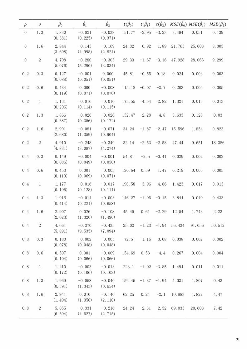
91
𝜌 𝜎 ��0 ��1 ��2 𝑡(��0) 𝑡(��1) 𝑡(��2) 𝑀𝑆𝐸(��0) 𝑀𝑆𝐸(��1) 𝑀𝑆𝐸(��2)
0 1.3 1.830
(0.381)
-0.021
(0.225)
-0.038
(0.371)
151.77 -2.95 -3.23 3.494 0.051 0.139
0 1.6 2.844
(3.698)
-0.145
(4.998)
-0.169
(2.824)
24.32 -0.92 -1.89 21.765 25.003 8.005
0 2 4.708
(5.076)
-0.280
(5.290)
-0.303
(3.034)
29.33 -1.67 -3.16 47.928 28.063 9.299
0.2 0.3 0.127
(0.088)
-0.001
(0.051)
0.000
(0.051)
45.81 -0.55 0.18 0.024 0.003 0.003
0.2 0.6 0.434
(0.119)
0.000
(0.071)
-0.008
(0.070)
115.18 -0.07 -3.7 0.203 0.005 0.005
0.2 1 1.131
(0.206)
-0.016
(0.114)
-0.010
(0.115)
173.55 -4.54 -2.82 1.321 0.013 0.013
0.2 1.3 1.866
(0.387)
-0.026
(0.356)
-0.026
(0.172)
152.47 -2.28 -4.8 3.633 0.128 0.03
0.2 1.6 2.901
(2.680)
-0.081
(1.359)
-0.071
(0.904)
34.24 -1.87 -2.47 15.596 1.854 0.823
0.2 2 4.910
(4.831)
-0.248
(3.097)
-0.349
(4.274)
32.14 -2.53 -2.58 47.44 9.651 18.386
0.4 0.3 0.149
(0.086)
-0.004
(0.049)
-0.001
(0.050)
54.81 -2.5 -0.41 0.029 0.002 0.002
0.4 0.6 0.453
(0.119)
0.001
(0.069)
-0.003
(0.071)
120.64 0.59 -1.47 0.219 0.005 0.005
0.4 1 1.177
(0.195)
-0.016
(0.128)
-0.017
(0.111)
190.58 -3.96 -4.86 1.423 0.017 0.013
0.4 1.3 1.916
(0.414)
-0.014
(0.221)
-0.003
(0.658)
146.27 -1.95 -0.15 3.844 0.049 0.433
0.4 1.6 2.907
(2.023)
0.026
(1.320)
-0.108
(1.490)
45.45 0.61 -2.29 12.54 1.743 2.23
0.4 2 4.661
(5.891)
-0.370
(9.535)
-0.435
(7.094)
25.02 -1.23 -1.94 56.434 91.056 50.512
0.8 0.3 0.180
(0.078)
-0.002
(0.048)
-0.005
(0.048)
72.5 -1.16 -3.08 0.038 0.002 0.002
0.8 0.6 0.507
(0.104)
0.001
(0.066)
-0.009
(0.066)
154.69 0.53 -4.4 0.267 0.004 0.004
0.8 1 1.210
(0.172)
-0.003
(0.106)
-0.013
(0.103)
223.1 -1.02 -3.85 1.494 0.011 0.011
0.8 1.3 1.969
(0.391)
-0.058
(1.343)
-0.040
(0.654)
159.45 -1.37 -1.94 4.031 1.807 0.43
0.8 1.6 2.941
(1.494)
0.010
(1.350)
-0.140
(2.110)
62.25 0.24 -2.1 10.883 1.822 4.47
0.8 2 5.055
(6.594)
-0.331
(4.527)
-0.216
(2.715)
24.24 -2.31 -2.52 69.035 20.603 7.42
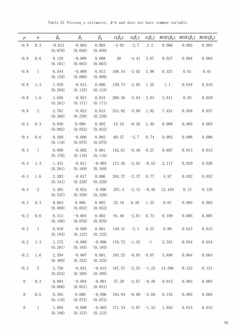
92
Table 21 Poisson_s estimator, 𝜆=4 and does not have common variable
𝜌 𝜎 ��0 ��1 ��2 𝑡(��0) 𝑡(��1) 𝑡(��2) 𝑀𝑆𝐸(��0) 𝑀𝑆𝐸(��1) 𝑀𝑆𝐸(��2)
-0.8 0.3 -0.012
(0.079)
-0.004
(0.050)
0.003
(0.050)
-4.92 -2.7 2.2 0.006 0.003 0.003
-0.8 0.6 0.128
(0.101)
-0.009
(0.065)
0.008
(0.065)
40 -4.41 3.87 0.027 0.004 0.004
-0.8 1 0.544
(0.159)
-0.009
(0.099)
0.012
(0.099)
108.54 -3.02 3.98 0.321 0.01 0.01
-0.8 1.3 1.029
(0.204)
-0.012
(0.133)
0.006
(0.133)
159.73 -2.85 1.55 1.1 0.018 0.018
-0.8 1.6 1.656
(0.261)
-0.021
(0.171)
0.015
(0.171)
200.36 -3.94 2.83 2.811 0.03 0.029
-0.8 2 2.701
(0.368)
-0.023
(0.239)
0.015
(0.239)
231.82 -3.09 1.92 7.431 0.058 0.057
-0.4 0.3 0.040
(0.082)
0.000
(0.052)
0.002
(0.052)
15.54 -0.26 1.49 0.008 0.003 0.003
-0.4 0.6 0.260
(0.119)
-0.006
(0.075)
0.002
(0.075)
69.27 -2.7 0.74 0.082 0.006 0.006
-0.4 1 0.809
(0.179)
-0.002
(0.116)
0.001
(0.116)
142.61 -0.48 0.27 0.687 0.013 0.013
-0.4 1.3 1.431
(0.261)
-0.011
(0.169)
-0.003
(0.169)
173.56 -2.03 -0.52 2.117 0.029 0.028
-0.4 1.6 2.203
(0.341)
-0.017
(0.228)
0.006
(0.228)
204.27 -2.37 0.77 4.97 0.052 0.052
-0.4 2 3.485
(0.547)
-0.024
(0.359)
-0.006
(0.359)
201.4 -2.12 -0.49 12.444 0.13 0.129
-0.2 0.3 0.063
(0.080)
0.000
(0.052)
0.002
(0.052)
25.16 0.26 1.35 0.01 0.003 0.003
-0.2 0.6 0.312
(0.108)
-0.004
(0.070)
0.002
(0.070)
91.46 -2.01 0.73 0.109 0.005 0.005
-0.2 1 0.918
(0.194)
-0.008
(0.122)
0.001
(0.122)
149.41 -2.1 0.25 0.88 0.015 0.015
-0.2 1.3 1.572
(0.281)
-0.009
(0.185)
-0.006
(0.185)
176.72 -1.52 -1 2.551 0.034 0.034
-0.2 1.6 2.394
(0.409)
-0.007
(0.252)
0.001
(0.252)
185.25 -0.93 0.07 5.896 0.064 0.063
-0.2 2 3.756
(0.633)
-0.031
(0.389)
-0.015
(0.389)
187.57 -2.53 -1.23 14.506 0.152 0.151
0 0.3 0.094
(0.080)
-0.004
(0.051)
-0.001
(0.051)
37.29 -2.67 -0.36 0.015 0.003 0.003
0 0.6 0.365
(0.110)
0.000
(0.072)
-0.006
(0.072)
104.94 -0.09 -2.69 0.145 0.005 0.005
0 1 1.005
(0.186)
-0.008
(0.123)
-0.005
(0.123)
171.34 -2.07 -1.33 1.045 0.015 0.015
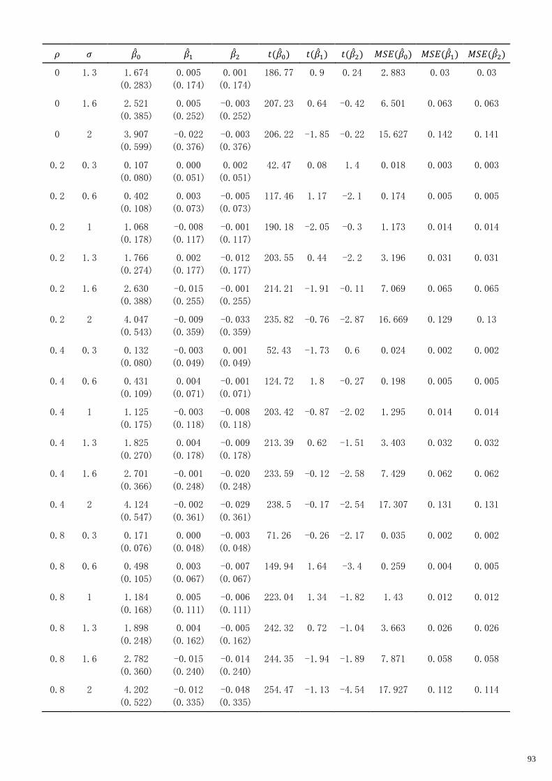
93
𝜌 𝜎 ��0 ��1 ��2 𝑡(��0) 𝑡(��1) 𝑡(��2) 𝑀𝑆𝐸(��0) 𝑀𝑆𝐸(��1) 𝑀𝑆𝐸(��2)
0 1.3 1.674
(0.283)
0.005
(0.174)
0.001
(0.174)
186.77 0.9 0.24 2.883 0.03 0.03
0 1.6 2.521
(0.385)
0.005
(0.252)
-0.003
(0.252)
207.23 0.64 -0.42 6.501 0.063 0.063
0 2 3.907
(0.599)
-0.022
(0.376)
-0.003
(0.376)
206.22 -1.85 -0.22 15.627 0.142 0.141
0.2 0.3 0.107
(0.080)
0.000
(0.051)
0.002
(0.051)
42.47 0.08 1.4 0.018 0.003 0.003
0.2 0.6 0.402
(0.108)
0.003
(0.073)
-0.005
(0.073)
117.46 1.17 -2.1 0.174 0.005 0.005
0.2 1 1.068
(0.178)
-0.008
(0.117)
-0.001
(0.117)
190.18 -2.05 -0.3 1.173 0.014 0.014
0.2 1.3 1.766
(0.274)
0.002
(0.177)
-0.012
(0.177)
203.55 0.44 -2.2 3.196 0.031 0.031
0.2 1.6 2.630
(0.388)
-0.015
(0.255)
-0.001
(0.255)
214.21 -1.91 -0.11 7.069 0.065 0.065
0.2 2 4.047
(0.543)
-0.009
(0.359)
-0.033
(0.359)
235.82 -0.76 -2.87 16.669 0.129 0.13
0.4 0.3 0.132
(0.080)
-0.003
(0.049)
0.001
(0.049)
52.43 -1.73 0.6 0.024 0.002 0.002
0.4 0.6 0.431
(0.109)
0.004
(0.071)
-0.001
(0.071)
124.72 1.8 -0.27 0.198 0.005 0.005
0.4 1 1.125
(0.175)
-0.003
(0.118)
-0.008
(0.118)
203.42 -0.87 -2.02 1.295 0.014 0.014
0.4 1.3 1.825
(0.270)
0.004
(0.178)
-0.009
(0.178)
213.39 0.62 -1.51 3.403 0.032 0.032
0.4 1.6 2.701
(0.366)
-0.001
(0.248)
-0.020
(0.248)
233.59 -0.12 -2.58 7.429 0.062 0.062
0.4 2 4.124
(0.547)
-0.002
(0.361)
-0.029
(0.361)
238.5 -0.17 -2.54 17.307 0.131 0.131
0.8 0.3 0.171
(0.076)
0.000
(0.048)
-0.003
(0.048)
71.26 -0.26 -2.17 0.035 0.002 0.002
0.8 0.6 0.498
(0.105)
0.003
(0.067)
-0.007
(0.067)
149.94 1.64 -3.4 0.259 0.004 0.005
0.8 1 1.184
(0.168)
0.005
(0.111)
-0.006
(0.111)
223.04 1.34 -1.82 1.43 0.012 0.012
0.8 1.3 1.898
(0.248)
0.004
(0.162)
-0.005
(0.162)
242.32 0.72 -1.04 3.663 0.026 0.026
0.8 1.6 2.782
(0.360)
-0.015
(0.240)
-0.014
(0.240)
244.35 -1.94 -1.89 7.871 0.058 0.058
0.8 2 4.202
(0.522)
-0.012
(0.335)
-0.048
(0.335)
254.47 -1.13 -4.54 17.927 0.112 0.114

94
Table 22 Poisson_f estimator, 𝜆=4 and does not have common variable
𝜌 𝜎 ��0 ��1 ��2 𝑡(��0) 𝑡(��1) 𝑡(��2) 𝑀𝑆𝐸(��0) 𝑀𝑆𝐸(��1) 𝑀𝑆𝐸(��2)
-0.8 0.3 0.089
(0.072)
-0.002
(0.043)
0.001
(0.072)
39.31 -1.22 0.45 0.013 0.002 0.005
-0.8 0.6 0.359
(0.098)
-0.004
(0.064)
0.002
(0.098)
116.36 -1.84 0.71 0.139 0.004 0.01
-0.8 1 0.999
(0.163)
-0.002
(0.103)
-0.001
(0.163)
194.39 -0.61 -0.19 1.025 0.011 0.026
-0.8 1.3 1.686
(0.247)
-0.007
(0.165)
0.001
(0.247)
215.76 -1.26 0.13 2.902 0.027 0.061
-0.8 1.6 2.539
(0.362)
-0.023
(0.243)
0.012
(0.362)
221.95 -2.93 1.09 6.576 0.059 0.131
-0.8 2 3.929
(0.553)
-0.011
(0.355)
-0.011
(0.553)
224.48 -1.01 -0.63 15.743 0.126 0.306
-0.4 0.3 0.089
(0.070)
0.000
(0.044)
0.001
(0.070)
40.31 -0.1 0.64 0.013 0.002 0.005
-0.4 0.6 0.359
(0.103)
-0.002
(0.064)
-0.001
(0.103)
110.47 -1.12 -0.28 0.14 0.004 0.011
-0.4 1 0.993
(0.161)
-0.002
(0.107)
0.000
(0.161)
195.34 -0.55 -0.09 1.013 0.012 0.026
-0.4 1.3 1.685
(0.236)
-0.002
(0.159)
-0.009
(0.236)
225.72 -0.36 -1.25 2.895 0.025 0.056
-0.4 1.6 2.543
(0.346)
-0.012
(0.232)
-0.004
(0.346)
232.41 -1.65 -0.41 6.588 0.054 0.12
-0.4 2 3.933
(0.542)
-0.011
(0.367)
-0.019
(0.542)
229.34 -0.95 -1.1 15.763 0.135 0.294
-0.2 0.3 0.088
(0.070)
0.000
(0.045)
0.002
(0.070)
39.75 -0.03 0.91 0.013 0.002 0.005
-0.2 0.6 0.359
(0.095)
-0.001
(0.062)
0.002
(0.095)
118.98 -0.58 0.5 0.138 0.004 0.009
-0.2 1 1.000
(0.165)
-0.004
(0.107)
-0.001
(0.165)
191.51 -1.32 -0.23 1.027 0.011 0.027
-0.2 1.3 1.685
(0.249)
-0.007
(0.169)
-0.005
(0.249)
214.28 -1.28 -0.62 2.901 0.028 0.062
-0.2 1.6 2.547
(0.363)
-0.008
(0.232)
-0.007
(0.363)
221.66 -1.06 -0.58 6.617 0.054 0.132
-0.2 2 3.942
(0.557)
-0.030
(0.346)
-0.014
(0.557)
223.77 -2.71 -0.77 15.852 0.121 0.311
0 0.3 0.093
(0.071)
-0.003
(0.046)
0.000
(0.071)
41.36 -2.33 0.06 0.014 0.002 0.005
0 0.6 0.363
(0.099)
0.001
(0.064)
-0.006
(0.099)
115.82 0.51 -2.02 0.142 0.004 0.01
0 1 1.007
(0.161)
-0.006
(0.108)
-0.006
(0.161)
197.55 -1.85 -1.21 1.04 0.012 0.026

95
𝜌 𝜎 ��0 ��1 ��2 𝑡(��0) 𝑡(��1) 𝑡(��2) 𝑀𝑆𝐸(��0) 𝑀𝑆𝐸(��1) 𝑀𝑆𝐸(��2)
0 1.3 1.670
(0.249)
0.008
(0.157)
0.003
(0.249)
212.28 1.59 0.36 2.852 0.025 0.062
0 1.6 2.524
(0.347)
0.002
(0.227)
0.005
(0.347)
229.92 0.22 0.42 6.489 0.051 0.12
0 2 3.922
(0.544)
-0.028
(0.343)
0.002
(0.544)
227.89 -2.58 0.09 15.682 0.118 0.296
0.2 0.3 0.088
(0.071)
-0.001
(0.046)
0.002
(0.071)
39.26 -0.39 0.77 0.013 0.002 0.005
0.2 0.6 0.358
(0.097)
0.003
(0.065)
-0.002
(0.097)
116.56 1.24 -0.59 0.137 0.004 0.009
0.2 1 1.005
(0.158)
-0.010
(0.107)
0.000
(0.158)
201.17 -3 0.02 1.035 0.011 0.025
0.2 1.3 1.682
(0.248)
0.001
(0.162)
-0.006
(0.248)
214.61 0.24 -0.79 2.889 0.026 0.061
0.2 1.6 2.539
(0.346)
-0.019
(0.231)
0.003
(0.346)
231.84 -2.66 0.32 6.566 0.054 0.12
0.2 2 3.927
(0.503)
-0.006
(0.338)
-0.020
(0.503)
246.68 -0.6 -1.24 15.679 0.114 0.254
0.4 0.3 0.091
(0.072)
-0.003
(0.044)
0.002
(0.072)
39.7 -2.15 0.83 0.013 0.002 0.005
0.4 0.6 0.354
(0.099)
0.002
(0.065)
0.001
(0.099)
112.78 0.95 0.35 0.135 0.004 0.01
0.4 1 1.006
(0.162)
-0.006
(0.109)
-0.005
(0.162)
196.44 -1.73 -0.94 1.039 0.012 0.026
0.4 1.3 1.682
(0.249)
-0.001
(0.164)
-0.003
(0.249)
213.26 -0.19 -0.42 2.891 0.027 0.062
0.4 1.6 2.541
(0.338)
-0.006
(0.232)
-0.015
(0.338)
237.6 -0.8 -1.44 6.569 0.054 0.115
0.4 2 3.939
(0.522)
-0.005
(0.347)
-0.021
(0.522)
238.42 -0.47 -1.26 15.787 0.121 0.273
0.8 0.3 0.092
(0.071)
-0.002
(0.044)
-0.001
(0.071)
40.88 -1.11 -0.39 0.014 0.002 0.005
0.8 0.6 0.358
(0.103)
0.001
(0.066)
0.000
(0.103)
110.35 0.4 -0.05 0.139 0.004 0.011
0.8 1 0.998
(0.163)
-0.002
(0.108)
-0.001
(0.163)
193.02 -0.51 -0.16 1.022 0.012 0.027
0.8 1.3 1.678
(0.244)
0.000
(0.161)
0.004
(0.244)
217.25 0.02 0.53 2.875 0.026 0.06
0.8 1.6 2.548
(0.362)
-0.021
(0.238)
-0.002
(0.362)
222.66 -2.75 -0.16 6.622 0.057 0.131
0.8 2 3.956
(0.522)
-0.017
(0.332)
-0.037
(0.522)
239.83 -1.66 -2.25 15.92 0.11 0.273