viii. poisson regression with multiple explanatory variables. generalization of poisson regression...

VIII. POISSON REGRESSION WITH MULTIPLE EXPLANATORY VARIABLES.

Generalization of Poisson regression model to include multiple covariates

Analyzing a complex survival data set with Poisson regression

Residual analysis

Deriving relative risk estimates from Poisson regression models

The Framingham data set Adjusting for confounding variables Adding interaction terms

© William D. Dupont, 2010Use of this file is restricted by a Creative Commons Attribution Non-Commercial Share Alike license.See http://creativecommons.org/about/licenses for details.

1. The Multiple Poisson Regression Model

Suppose that data on patients (or patient-years of follow-up) can be logically grouped into J strata based on age or other factors.

Let j = 1,…,J denote the patient’s strata.

Suppose that patients in strata j may be grouped into K exposure categories denoted by k = 1,…, K.

Let be explanatory variables that describe the kth exposure group of patients in strata j, and

x x xjk jk jkp1 2, ,...,

( )1 2, , ...,jk jk jk jkpx x xx = denote the values of all of the covariates for patients in the jth strata and kth exposure category.

jk be the probability that someone in strata j and exposure group k will die.

Then the multiple Poisson regression model assumes that

1 1 2 2log E | log ...jk jk jk j jk jk p jkpd n x x xxé ùé ù é ù= +a +b +b + +bë û ë ûë û

where

1, , Ja a are unknown nuisance parameters, and

1 2, , ..., pb b bare unknown parameters of interest.

njk is the number of patients at risk in the jth strata who are in exposure group k

djk is the number of deaths (events) among these patients. djk is assumed to have a Poisson distribution with mean njk jk ,

,

{8.1}

For example, suppose that there are

J = 5 = five age strata.

and that patients are classified as light or heavy drinkers and light or heavy smokers in each strata. Then the are

K = 4 exposure categories (2 drinking categories times 2 smoking categories).

x xjk1 1 RST1: Patient is heavy drinker

0: Patient is light drinker

x xjk2 2 RST1: Patient is heavy smoker

0: Patient is light smoker

We might choose

p = 2 and let

1 1 2 2log( ( )) log( )jk jk j jk jkE d n x x= +a + b + b

Then the Poisson regression model is

where

j = 1, 2, … , 5;

k = 1, 2, 3, 4.

k = 1 k = 2 k = 3 k = 4

K = 4 J = 5 p = 2

Light Drinker Light Smoker

x1 = 0 x 2 = 0

Light Drinker Heavy Smoker

x1 = 0 x 2 = 1

Heavy Drinker Light Smoker

x1 = 1 x 2 = 0

Heavy Drinker Heavy Smoker

x1 = 1 x 2 = 1

j = 1 …x141 = x 1 = 1

x142 = x 2 = 1

j = 2 = 0 x211 = x 1

x212 = x 2 = 0… …

AG

E

j = 3x321 = x 1 = 0

x322 = x 2 = 1… …

j = 4x431 = x 1 = 1

x432 = x 2 = 0…

j = 5 …x541 = x 1 = 1

x542 = x 2 = 1

= 0 x311 = x 1

x312 = x 2 = 0

= 0 x411 = x 1

x412 = x 2 = 0

= 0 x511 = x 1

x512 = x 2 = 0

= 0 x111 = x 1

x112 = x 2 = 0

x221 = x 1 = 0

x222 = x 2 = 1

x121 = x 1 = 0

x122 = x 2 = 1

x421 = x 1 = 0

x422 = x 2 = 1

x521 = x 1 = 0

x522 = x 2 = 1

Note that if we subtract from both sides of {8.1} we get

{8.2}

Two patient groups with covariates and

will have log probabilities1 2, ,...,jk jk jk px x x

1 2, ,...,jk jk jkpx x x

log( ) ... jk j jk jk jk p px x x 1 1 2 2

log( ) ... jk j jk jk jkp px x x 1 1 2 2

log( )n jk

log( ( )/ )E d njk jk

log( ) ... jk j jk jk jkp px x x 1 1 2 2

log( / ) jk jk

( ) ( ) ... ( )x x x x x xjk jk jk jk jk p jkp p 1 1 1 2 2 2

Subtracting the latter equation from the former gives

{8.3}

Thus, we can estimate log relative risks in Poisson regression models in precisely the same way that we estimated log odds ratios in logistic regression.

Indeed, the only difference is that in logistic regression weighted sums of model coefficients are interpreted as log odds ratios while in Poisson regression they are interpreted as log relative risks.

This is a person-time data set

The covariates areBMI grouped in quartilesSerum cholesterol grouped in quartilesDBP grouped in quartilesgenderage < 45, 46 – 50, …, 76 – 80, > 80

For each unique combination of covariate values we also have

pt_yrs the number of patient-years of follow-up for patients with these covariate values

chd_cnt the number of coronary heart disease events observed in these patient-years of follow-up

2. The 8.12.Framingham.dta Data Set

2 patient-years of follow-up to the record for his covariate values and age 41 – 45,

5 patient-years of follow-up to the record for his covariate values and age 46 – 50, and

1 patient-year of follow-up to the record for his covariate values and age 51 – 55

A patient who enters on his 44th birthday and exits at age 51 with CHD will contribute

He contributes

1 CHD event to the record for his covariate values and age 51 – 55

3. Gender, Age and CHD in the Framingham Heart Study

a) Analyzing the multiplicative model with Stata

. * 9.3.Framingham.log

. *

. * Estimate the effect of age and gender on coronary heart disease CHD)

. * using several Poisson regression models (Levy 1999).

. *

. use C:\WDDtext\8.12.Framingham.dta, clear

. *

. * Fit multiplicative model of effect of gender and age on CHD

. *

. * Statistics > Generalized linear models > Generalized linear models (GLM)

. glm chd_cnt i.age_gr male, family(poisson) link(log) {1}> lnoffset(pt_yrs) eform

{1} We fit the model log( ( _ )) log( _ )E chd cnt pt yrs= +a

. _ . _ ... . _2 3 950 age gr 55 age gr 81 age gr male

Generalized linear models No. of obs = 1267Optimization : ML: Newton-Raphson Residual df = 1257 Scale parameter = 1Deviance = 1391.341888 (1/df) Deviance = 1.106875Pearson = 1604.542689 (1/df) Pearson = 1.276486

Variance function: V(u) = u [Poisson]Link function : g(u) = ln(u) [Log]Standard errors : OIM

Log likelihood = -1559.206456 AIC = 2.477043BIC = -7589.177938------------------------------------------------------------------------------ chd_cnt | IRR Std. Err. z P>|z| [95% Conf. Interval]-------------+---------------------------------------------------------------- age_gr | 50 | 1.864355 .3337745 3.48 0.001 1.312618 2.648005 55 | 3.158729 .5058088 7.18 0.000 2.307858 4.323303 60 | 4.885053 .7421312 10.44 0.000 3.627069 6.579347 65 | 6.44168 .9620181 12.47 0.000 4.807047 8.632168 70 | 6.725369 1.028591 12.46 0.000 4.983469 9.076127 75 | 8.612712 1.354852 13.69 0.000 6.327596 11.72306 80 | 10.37219 1.749287 13.87 0.000 7.452702 14.43534 81 | 13.67189 2.515296 14.22 0.000 9.532967 19.60781 | male | 1.996012 .1051841 13.12 0.000 1.800144 2.213192 pt_yrs | (exposure)------------------------------------------------------------------------------

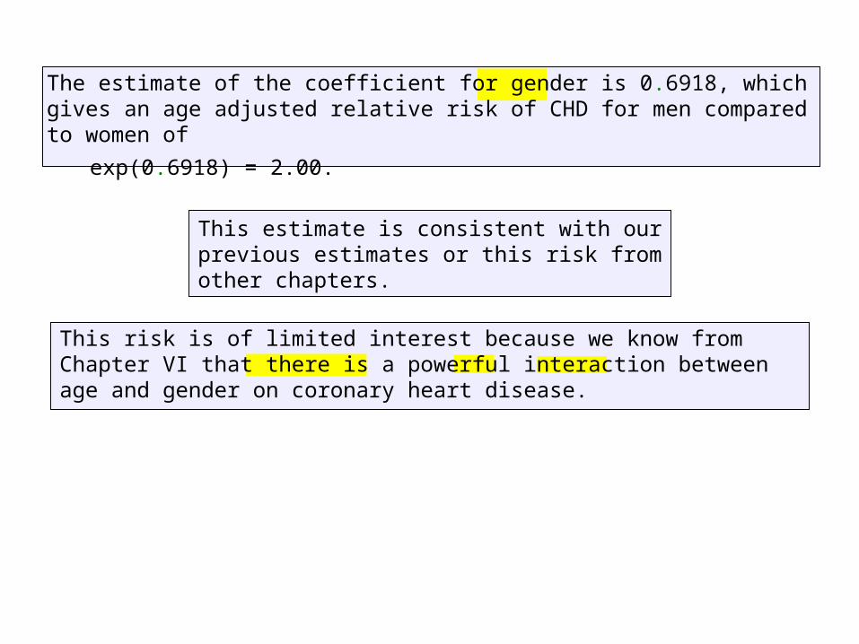
This estimate is consistent with our previous estimates or this risk from other chapters.

This risk is of limited interest because we know from Chapter VI that there is a powerful interaction between age and gender on coronary heart disease.

The estimate of the coefficient for gender is 0.6918, which gives an age adjusted relative risk of CHD for men compared to women of

exp(0.6918) = 2.00.

b) Age-sex specific incidence of CHD

Let us next plot the age specific incidence of CHD in men and women. 9.3.Framingham.log continues.

. *

. * Tabulate patient-years of follow-up and number of

. * CHD events by sex and age group.

. *

. * Statistics > Summaries... > Tables > Table of summary statistics (table)

. table sex, contents(sum pt_yrs sum chd_cnt) by(age_gr) ----------+---------------------------Age Group |and Sex | sum(pt_yrs) sum(chd_cnt)----------+---------------------------<= 45 | Men | 7370 43 Women | 9205 9----------+---------------------------45-50 | Men | 5835 53 Women | 7595 25----------+---------------------------50-55 | Men | 6814 110 Women | 9113 46----------+---------------------------55-60 | Men | 7184 155 Women | 10139 105----------+---------------------------

----------+---------------------------60-65 | Men | 6678 178 Women | 9946 148----------+---------------------------65-70 | Men | 4557 121 Women | 7385 120----------+---------------------------70-75 | Men | 2575 94 Women | 4579 88----------+---------------------------75-80 | Men | 1205 50 Women | 2428 59----------+---------------------------> 80 | Men | 470 19 Women | 1383 50--------------------------------------

. *

. * Calculate age-sex specific incidence of CHD

. *

. * Data > Create... > Other variable-trans... > Make dataset of means...

. collapse (sum) patients = pt_yrs chd = chd_cnt, by(age_gr male) {1}

{1} Collapse the data file to one record for each combination of age_gr and sex. Let patients be the total number of patient-years of follow-up and let chd be the total number CHD events in these groups.

. generate rate = 1000*chd/patients {2}

. generate men = rate if male==1(9 missing values generated)

. generate women = rate if male==0(9 missing values generated)

.* Graphics > Bar chart

. graph bar men women, over(age_gr) ytitle(CHD Morbidity Rate per 1000) /// {3}> ylabel(0(5)40, angle(0)) subtitle(Age, position(6)) ///> legend(order(1 "Men" 2 "Women") ring(0) position(11) col(1))

{2} rate is the age-sex specific incidence rate of CHD per year per 1,000.

{3} The bar option specifies that a bar graph is to be produced. The two variables men and women together with the over(age_gr) option specify that a grouped bar graph of men and women stratified by age_gr is to be drawn. The y-axis is the mean of the values of men and women in all records with identical values of age_gr. However, in this particular example, there is only one non-missing value of men and women for each age group.

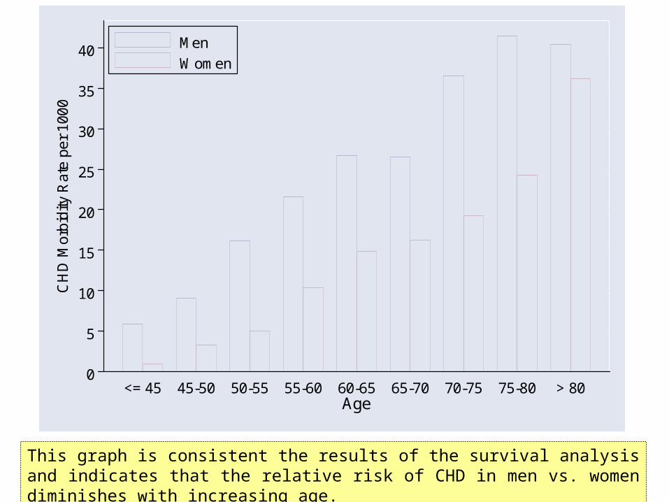
This graph is consistent the results of the survival analysis and indicates that the relative risk of CHD in men vs. women diminishes with increasing age.

0

5

10

15

20

25

30

35

40C

HD

Mor

bidi

ty R

ate

per

1000

<= 45 45-50 50-55 55-60 60-65 65-70 70-75 75-80 > 80Age

Men

Women

c) Using Poisson regression to model the effects of gender and age on CHD risk

Let us now model this relationship. 9.3.Framingham.log continues.

. use C:\WDDtext\8.12.Framingham.dta, clear {1}

. *

. * Add interaction terms to the model

. *


. glm chd_cnt age_gr##male, family(poisson) link(log) lnoffset(pt_yrs) {2}

{1} In creating the preceding bar graph we collapsed the data set. We need to restore the original data set before preceding.

{2} In this model we add 9 interaction terms of the form50.age_gr#1.male = 50.age_gr1.male,55.age_gr#1.male = 55.age_gr1.male,

.

.

.80.age_gr#1.male = 80.age_gr1.male, and81.age_gr#1.male = 81.age_gr1.male.

The syntax is identical to that used in Chapter IV.

Iteration 0: log likelihood = -1621.7301 Iteration 1: log likelihood = -1547.0628 Iteration 2: log likelihood = -1544.3498 Iteration 3: log likelihood = -1544.3226 Iteration 4: log likelihood = -1544.3226



Log likelihood = -1544.322566 AIC = 2.466176BIC = -7561.790461

------------------------------------------------------------------------------ chd_cnt | Coef. Std. Err. z P>|z| [95% Conf. Interval]-------------+---------------------------------------------------------------- age_gr | 50 | 1.213908 .3887301 3.12 0.002 .4520112 1.975805 55 | 1.641462 .3644863 4.50 0.000 .9270817 2.355842 60 | 2.360093 .3473254 6.80 0.000 1.679348 3.040838 65 | 2.722564 .3433189 7.93 0.000 2.049671 3.395457 70 | 2.810563 .3456074 8.13 0.000 2.133185 3.487941 75 | 2.978378 .3499639 8.51 0.000 2.292462 3.664295 80 | 3.212992 .3578551 8.98 0.000 2.511609 3.914375 81 | 3.61029 .3620927 9.97 0.000 2.900602 4.319979 | 1.male | 1.786305 .3665609 4.87 0.000 1.067858 2.504751 | age_gr#male | 50 1 | -.771273 .4395848 -1.75 0.079 -1.632843 .0902975 55 1 | -.623743 .4064443 -1.53 0.125 -1.420359 .1728731 60 1 | -1.052307 .3877401 -2.71 0.007 -1.812263 -.2923503 65 1 | -1.203381 .3830687 -3.14 0.002 -1.954182 -.4525805 70 1 | -1.295219 .3885418 -3.33 0.001 -2.056747 -.5336915 75 1 | -1.144716 .395435 -2.89 0.004 -1.919754 -.3696772 80 1 | -1.251231 .4139035 -3.02 0.003 -2.062467 -.4399949 81 1 | -1.674611 .4549709 -3.68 0.000 -2.566338 -.7828845 | _cons | -6.930278 .3333333 -20.79 0.000 -7.583599 -6.276956 pt_yrs | (exposure)------------------------------------------------------------------------------

. lincom 1.male, irr {3} ( 1) [chd_cnt]male = 0 ------------------------------------------------------------------------------ chd_cnt | IRR Std. Err. z P>|z| [95% Conf. Interval]-------------+---------------------------------------------------------------- (1) | 5.96736 2.187401 4.87 0.000 2.909143 12.24051------------------------------------------------------------------------------

{3} The risk of CHD for a man < 45 years of age is 5.97 times that of a woman of comparable age.

. lincom 1.male + 50.age_gr#1.male, irr {4} ( 1) [chd_cnt]1.male + [chd_cnt]50.age_gr#1.male = 0 ------------------------------------------------------------------------------ chd_cnt | IRR Std. Err. z P>|z| [95% Conf. Interval]-------------+---------------------------------------------------------------- (1) | 2.759451 .6695176 4.18 0.000 1.715134 4.439635------------------------------------------------------------------------------

.

.

.

{4} The log incidence of CHD for a man aged 45-50 is

_cons + 1.male + 50.age_gr + 50.age_gr#1.male {8.4}

For women, the corresponding log incidence is

_cons + 50.age_gr {8.5}

Subtracting {8.5} from {8.4} gives that the log relative risk for men aged 45-50 compared to women of the same age is

1.male + 50.age_gr#1.male

We put these terms in the lincom statement to estimate the relative risk for men in this age group to be 2.76.

Similar lincom commands permit us to complete the following table.

AgeRelative

Risk

95% Confidence

IntervalMen Women Men Women

< 45 7,370 9,205 43 9 5.97 2.9 - 12

Patient-years of follow-up

CHD Events

Table 8.1. Age-specific relative risks of CHD in men compared to women (5 year age intervals).

> 80 470 1,383 19 50 1.12 0.66 - 1.9

46 - 50 5,835 7,595 53 25 2.76 1.7 - 4.451 - 55 6,814 9,113 110 46 3.20 2.3 - 4.5

56 - 60 7,184 10,139 155 105 2.08 1.6 - 2.7

61 - 65 6,678 9,946 178 148 1.79 1.4 - 2.266 - 70 4,557 7,385 121 120 1.63 1.3 - 2.171 - 75 2,575 4,579 94 88 1.90 1.4 - 2.576 - 80 1,205 2,428 50 59 1.71 1.2 - 2.5

From the preceding table it appears reasonable to collapse ages 46 - 55 into one interval, and ages 61 - 80 into another. We do this next as 9.3.Framingham.log continues.

. *

. * Refit model with interaction terms using fewer parameters.

. *

. generate age_gr2 = recode(age_gr, 45,55,60,80,81) {1}


. glm chd_cnt age_gr2##male ///> , family(poisson) link(log) lnoffset(pt_yrs) eform {2}




Log likelihood = -1563.826738 AIC = 2.484336 BIC = -7579.937

{1} This model is identical to the preceding one except that we have fewer age groups. We can generate the following table using lincom commands similar to those used to produce Table 8.1.

{2} eform exponentiates the coefficients in the output table

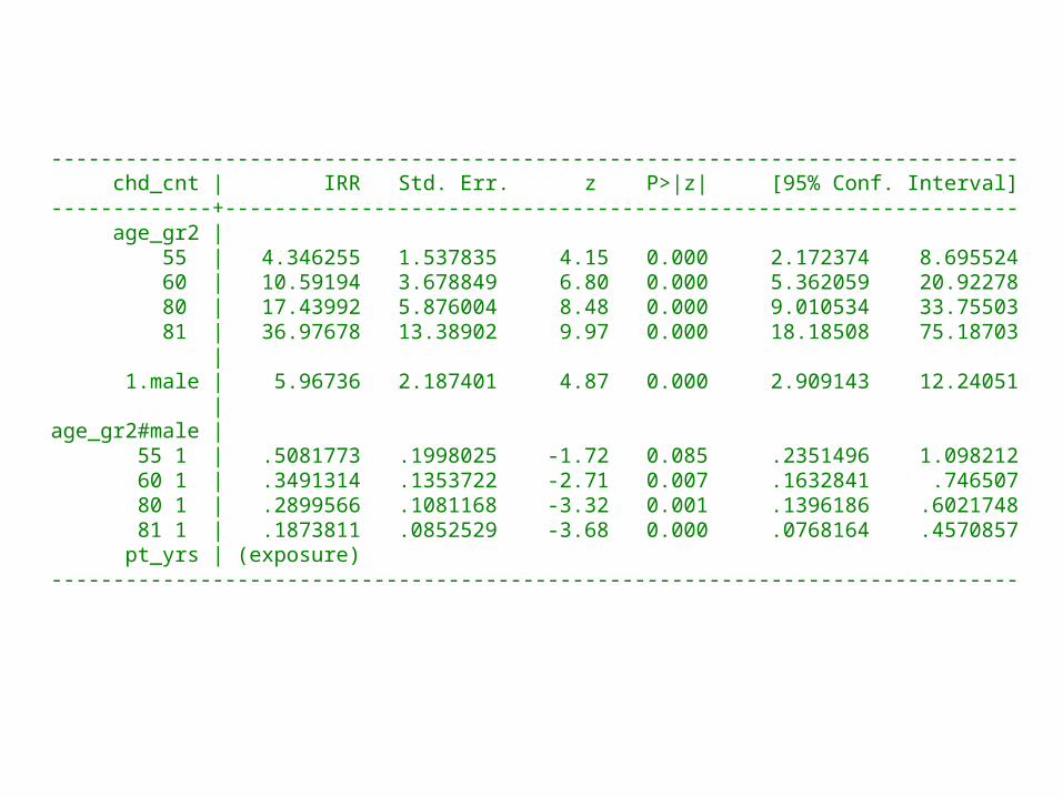
------------------------------------------------------------------------------ chd_cnt | IRR Std. Err. z P>|z| [95% Conf. Interval]-------------+---------------------------------------------------------------- age_gr2 | 55 | 4.346255 1.537835 4.15 0.000 2.172374 8.695524 60 | 10.59194 3.678849 6.80 0.000 5.362059 20.92278 80 | 17.43992 5.876004 8.48 0.000 9.010534 33.75503 81 | 36.97678 13.38902 9.97 0.000 18.18508 75.18703 | 1.male | 5.96736 2.187401 4.87 0.000 2.909143 12.24051 |age_gr2#male | 55 1 | .5081773 .1998025 -1.72 0.085 .2351496 1.098212 60 1 | .3491314 .1353722 -2.71 0.007 .1632841 .746507 80 1 | .2899566 .1081168 -3.32 0.001 .1396186 .6021748 81 1 | .1873811 .0852529 -3.68 0.000 .0768164 .4570857 pt_yrs | (exposure)------------------------------------------------------------------------------

. lincom 1.male + 55.age_gr2#1.male, irr

( 1) [chd_cnt]1.male + [chd_cnt]55.age_gr2#1.male = 0------------------------------------------------------------------------------ chd_cnt | IRR Std. Err. z P>|z| [95% Conf. Interval]-------------+---------------------------------------------------------------- (1) | 3.032477 .4312037 7.80 0.000 2.294884 4.007138------------------------------------------------------------------------------



This table suggests that men are at substantially increased risk of CHD compared to premenopausal women of the same age. After the menopause this risk ratio declines but remains significant until age 80. After age 80 there is no significant difference in CHD risk between men and women.

Age Relative Risk

95% Confidence


46 - 55 12,649 16,708 163 71 3.03 2.3 - 4.0

56 - 60 7,184 10,139 155 105 2.08 1.6 - 2.7

61 - 80 15,015 24,338 443 415 1.73 1.5 - 2.0

Patient-years of follow-up CHD Events

Table 8.2. Age-specific relative risks of CHD in men compared to women (variable age intervals).

> 80 470 1,383 19 50 1.12 0.66 - 1.9

< 45 7,370 9,205 43 9 5.97 2.9 - 12

d) Adjusting CHD risk for confounding variables

Of course Table 8.2 is based on observational data, and may be influenced by confounding variables. We next adjust these results for possible confounding due to body mass index, serum cholesterol, and diastolic blood pressure. 9.3. Framingham.log continues.

. table bmi_gr

---------------------- bmi_gr | Freq.----------+----------- 22.8 | 312 25.2 | 290 28 | 320 29 | 312----------------------

. *

. * The i. syntax only works for integer variables. bmi_gr gives the

. * quartile boundaries to one decimal place. We multiply this variable

. * by 10 in order to be able to use this syntax. Since indicator

. * covariates are entered into the model, multiplying by 10 will

. * not affect our estimates

. *

. gen bmi_gr10 = bmi_gr*10(33 missing values generated)

. *

. * Adjust analysis for body mass index (BMI)

. *


. glm chd_cnt age_gr2##male i.bmi_gr10 ///> , family(poisson) link(log) lnoffset(pt_yrs)




.

.

.

This model is nested within the preceding model and contains 3 more parameters. Therefore the reduction in model deviance will have an asymptotically 2 distribution with 3 degrees of freedom under the null hypothesis that the simpler model is correct.

This reduction is 1,401 - 1,328 = 73, which is overwhelmingly significant (P <10-14 ). We will leave i.bmi_gr10 in the model.

. *

. * Adjust estimates for BMI and serum cholesterol

. *


. glm chd_cnt age_gr2##male i.bmi_gr10 i.scl_gr ///> , family(poisson) link(log) lnoffset(pt_yrs)





The model deviance is reduced by 1,328 - 1208 = 120, which has a 2 distribution with 3 degrees of freedom with P <10-25.

. *

. * Adjust estimates for BMI serum cholesterol and

. * diastolic blood pressure

. *


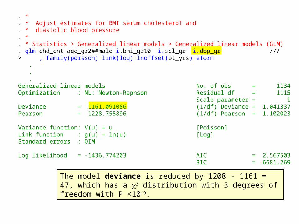
. glm chd_cnt age_gr2##male i.bmi_gr10 i.scl_gr i.dbp_gr ///> , family(poisson) link(log) lnoffset(pt_yrs) eform . . .Generalized linear models No. of obs = 1134Optimization : ML: Newton-Raphson Residual df = 1115 Scale parameter = 1Deviance = 1161.091086 (1/df) Deviance = 1.041337Pearson = 1228.755896 (1/df) Pearson = 1.102023



The model deviance is reduced by 1208 - 1161 = 47, which has a 2 distribution with 3 degrees of freedom with P <10-9.

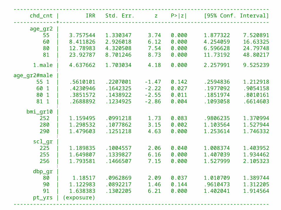
------------------------------------------------------------------------------ chd_cnt | IRR Std. Err. z P>|z| [95% Conf. Interval]-------------+---------------------------------------------------------------- age_gr2 | 55 | 3.757544 1.330347 3.74 0.000 1.877322 7.520891 60 | 8.411826 2.926018 6.12 0.000 4.254059 16.63325 80 | 12.78983 4.320508 7.54 0.000 6.596628 24.79748 81 | 23.92787 8.701246 8.73 0.000 11.73192 48.80217 |

1.male | 4.637662 1.703034 4.18 0.000 2.257991 9.525239 |

age_gr2#male | 55 1 | .5610101 .2207001 -1.47 0.142 .2594836 1.212918 60 1 | .4230946 .1642325 -2.22 0.027 .1977092 .9054158 80 1 | .3851572 .1438922 -2.55 0.011 .1851974 .8010161 81 1 | .2688892 .1234925 -2.86 0.004 .1093058 .6614603 |

bmi_gr10 | 252 | 1.159495 .0991218 1.73 0.083 .9806235 1.370994 280 | 1.298532 .1077862 3.15 0.002 1.103564 1.527944 290 | 1.479603 .1251218 4.63 0.000 1.253614 1.746332 |

scl_gr | 225 | 1.189835 .1004557 2.06 0.040 1.008374 1.403952 255 | 1.649807 .1339827 6.16 0.000 1.407039 1.934462 256 | 1.793581 .1466507 7.15 0.000 1.527999 2.105323 |

dbp_gr | 80 | 1.18517 .0962869 2.09 0.037 1.010709 1.389744 90 | 1.122983 .0892217 1.46 0.144 .9610473 1.312205 91 | 1.638383 .1302205 6.21 0.000 1.402041 1.914564 pt_yrs | (exposure)------------------------------------------------------------------------------

. lincom 1.male + 55.age_gr2#1.male, irr {1}




{1} We next use lincom statements in the same way as before to construct Table 8.3.

Table 8.3. Age-specific relative risks of CHD in men compared to women. Risks are adjusted for body mass index, serum cholesterol

and diastolic blood pressure.

AgeRelative

Risk

95% Confidence


Patient-years of follow-up CHD Events

46 - 55 12,649 16,708 163 7156 - 60 7,184 10,139 155 10561 - 80 15,015 24,338 443 415

> 80 470 1,383 19 50

< 45 7,370 9,205 43 9 4.64 2.3 – 9.52.60 2.0 - 3.4

1.96 1.5 - 2.51.79 1.6 - 2.0

1.25 0.73 - 2.1

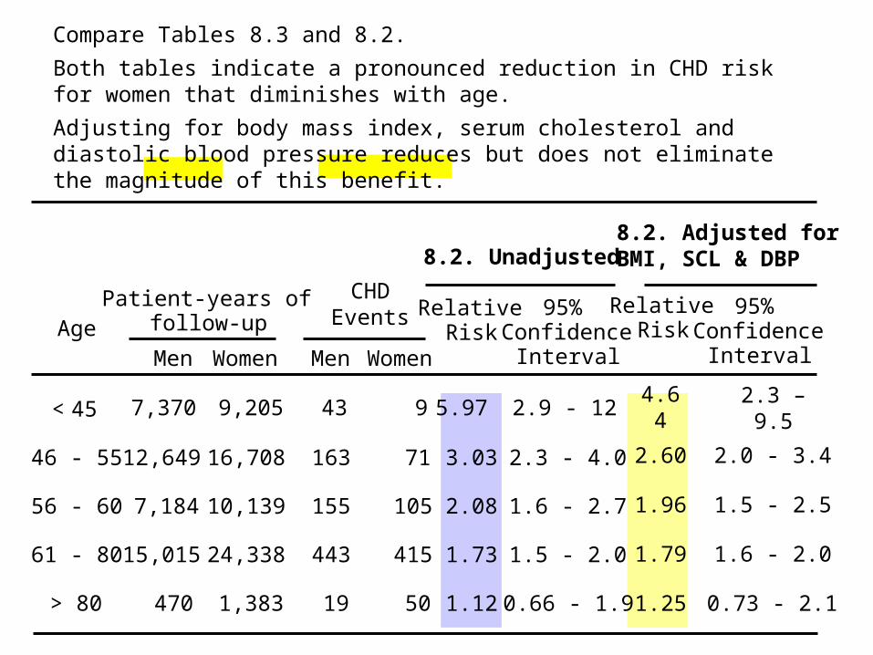
Compare Tables 8.3 and 8.2.

Both tables indicate a pronounced reduction in CHD risk for women that diminishes with age.

Adjusting for body mass index, serum cholesterol and diastolic blood pressure reduces but does not eliminate the magnitude of this benefit.

8.2. Unadjusted8.2. Adjusted forBMI, SCL & DBP

AgeRelative

Risk95%

Confidence IntervalMen Women Men Women

Patient-years of follow-up

CHDEvents

61 - 80 15,015 24,338 443 415 1.73 1.5 - 2.0

> 80 470 1,383 19 50 1.12 0.66 - 1.9

56 - 60 7,184 10,139 155 105 2.08 1.6 - 2.7

46 - 55 12,649 16,708 163 71 3.03 2.3 - 4.0 2.60 2.0 - 3.4

1.79 1.6 - 2.0

1.25 0.73 - 2.1

1.96 1.5 - 2.5

Relative Risk

95% Confidence

Interval

< 45 7,370 9,205 43 9 5.97 2.9 - 12 4.64 2.3 – 9.5

Adjusting for such variables is called overmatching and can cause a serious underestimate of the true relative risk.

One of the many ways we can go wrong is to confuse a true confounding variable with one that is on the causal pathway to the outcome of interest.

4. Confounding versus Overmatching

It cannot be overemphasized that the correct model depends on the biologic context and cannot be ascertained solely through mathematical analysis.

Consider the preceding example.

Such variables look like confounding variables in that they are correlated with both the exposure and disease outcome of interest.

We know that

· Low density serum cholesterol (LDSC) is an independent risk factor for CHD.

In this case adjusting for serum cholesterol may constitute overmatching and may falsely lower the relative risk of CHD for middle aged men.

Thus, it is plausible that the reduced CHD risk of premenopausal women results, in part, from a reduction in LDSC due to endogenous estrogens.

· Exogenous estrogens reduce LDSC, and

women who take hormonal replacement therapy have reduced risks of CHD.

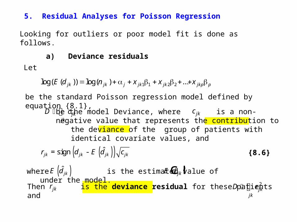
be the model Deviance, where is a non-negative value that represents the

contribution to the deviance of the group of patients with identical covariate values, and

D cjkjk

cjk

5. Residual Analyses for Poisson Regression

Looking for outliers or poor model fit is done as follows.

a) Deviance residuals

Let

log( ( )) log( ) ...E d n x x xjk jk j jk jk jkp p 1 1 2 2

be the standard Poisson regression model defined by equation {8.1},

rjk D rjkjk

2Then is the deviance residual for these patients and

( )( )ˆsignjk jk jk jkr d E d c= - {8.6}

E d jkc hwhere is the estimated value of under the model.

( )jkE d

As with Pearson residuals, deviance residuals are affected by varying degrees of leverage associated with the different covariate patterns. This leverage tends to shorten the residual by pulling the estimate of in the direction of .

ˆjkl

/jk jkd n

We can adjust for this shrinkage by calculating the standardized deviance residual

/ 1sjk jk jkr r h= -

where is the leverage of the covariate pattern.jkh thjk

If the model is correct, roughly 95% of these residuals should lie between + 2

However, many such records with residuals having the same sign may result in a poor model fit that does not show up in a residual analysis that calculates a separate residual for each identical record.

For this reason it is best to compress such records before analyzing our residuals.

It doesn’t matter how many records have identical covariates when we are fitting a Poisson regression model.

b) Residual analysis of CHD model of sex, age and other variables

9.3.Framingham.log continues. ** Compress data set for residual plot*. sort male bmi_gr scl_gr dbp_gr age_gr2 {1}. * Data > Create... > Other variable-trans... > Make dataset of means.... collapse (sum) pt_yrs=pt_yrs chd_cnt=chd_cnt, /// {2}> by (male bmi_gr10 scl_gr dbp_gr age_gr2)

{1} Before compressing the data file we must bring all records with identical covariates together. We do this with the sort command.

{2} This command combines all records with identical values of male, bmi_gr, scl_gr, dbp_gr3, and age_gr2 together. pt_yrs and chd_cnt denote the total number of patient-years of observation and total number of CHD events in these records, respectively.

. *

. * Re-analyze previous model using collapsed data set.

. *


. glm chd_cnt age_gr2##male i.bmi_gr10 i.scl_gr i.dbp_gr /// {3}> , family(poisson) link(log) lnoffset(pt_yrs) . . .Generalized linear models No. of obs = 623Optimization : ML: Newton-Raphson Residual df = 604 Scale parameter = 1Deviance = 600.7760472 (1/df) Deviance = .9946623 {4}Pearson = 633.8816072 (1/df) Pearson = 1.049473

Variance function: V(u) = u [Poisson]Link function : g(u) = ln(u) [Log]

AIC = 2.862427Log likelihood = -872.645946 BIC = -3285.69 . . .

{3} This command fits the same model used for Table 8.3.

{4} Collapsing the data set reduces the model deviance but has no effect on the model’s parameter estimates or their standard errors. The table of coefficients, standard errors and confidence intervals is not shown here (see the output from the last time we ran this model in Section 2c).

. *

. * Estimate the expected number of CHD events and the

. * standardized deviance residual for each record in the data set.

. *

. predict e_chd, mu {5}

(82 missing values generated)

{5} The mu option of this command defines e_chd to equal , the estimated expected number of deaths for each record. More generally, it calculates the inverse of the link function evaluated at the linear predictor for the given record. For Poisson regression this is the exponentiated value of the linear predictor.

( )E jkd

. predict dev, standardized deviance {6}

(82 missing values generated){6} This predict command calculates dev to equal the

standardized deviance residual.

. generate e_rate = 1000*e_chd/pt_yrs(82 missing values generated)

. label variable e_rate "Incidence of CHD per Thousand"

. *

. * Draw scatterplot of the standardized deviance residual versus the

. * estimated incidence of CHD. Include lowess regression curve on this plot.

. *

. * Graphics > Smoothing and densities > Lowess smoothing

. lowess dev e_rate, bwidth(0.2) msymbol(Oh) ylabel(-3(1)4) ytick(-3(0.5)4) /// {7}

> lineopts(color(red) lwidth(medthick)) yline(-2 0 2 , lcolor(blue)) /// {8}> xlabel(0(10)80) xtick(5(10)75)

{7} Plot a lowess regression of the standardized deviance residual against the expected number of CHD events.

{8} This lineopts option specifies the color and thickness of the regression line.

-3-2

-10

12

34

stan

dard

ized

dev

ianc

e re

sidu

al

0 10 20 30 40 50 60 70 80Incidence of CHD per Thousand

bandwidth = .2

Lowess smoother

The deviance residual plot indicates that the model fit is quite good, with most of the residuals lying between + 2.

There is a suggestion of a negative drift for residuals associated with a large numbers of expected CDH events.

The standard deviation of these residuals may also be lower than those associated with low event rates.

6. What we have covered

Generalization of Poisson regression model to include multiple covariates

Analyzing a complex survival data set with Poisson regression

Residual analysis

Deriving relative risk estimates from Poisson regression models

The family(poisson) and link(log) options of the glm command

The Framingham data set Adjusting for confounding variables Adding interaction terms

Deviance residuals The standardized deviance option of the predict

command.

Cited Reference

Levy D, National Heart Lung and Blood Institute., Center for Bio-Medical Communication. 50 Years of Discovery : Medical Milestones from the National Heart, Lung, and Blood Institute's Framingham Heart Study. Hackensack, N.J.: Center for Bio-Medical Communication Inc.; 1999.

For additional references on these notes see.

Dupont WD. Statistical Modeling for Biomedical Researchers: A Simple Introduction to the Analysis of Complex Data. 2nd ed. Cambridge, U.K.: Cambridge University Press; 2009.

viii. poisson regression with multiple explanatory variables. generalization of poisson regression...

Documents

j strata

strata j

patients strata

poisson distribution

heavy drinker heavy

light drinker heavy

heavy drinker light

light drinker light