07 handout.simple poisson regression
TRANSCRIPT
VII. INTRODUCTION TO POISSON REGRESSIONInferences on Morbidity and Mortality Rates
Elementary statistics involving rates Classical methods for deriving 95% confidence intervals for
relative risks Relationship between the binomial and Poisson distributions Poisson regression and 2x2 contingency tables Estimating relative risks from Poisson regression models
Poisson regression is an example of a generalized linear model
Poisson Regression and survival analysis
Incidence and relative risk
Offsets in Poisson regression models
Assumptions of the Poisson regression model Contrast between logistic and Poisson regression 95% confidence intervals for relative risk estimates
Converting survival records to person-year records with Stata
© William D. Dupont, 2010, 2011Use of this file is restricted by a Creative Commons Attribution Non-Commercial Share Alike license.See http://creativecommons.org/about/licenses for details.
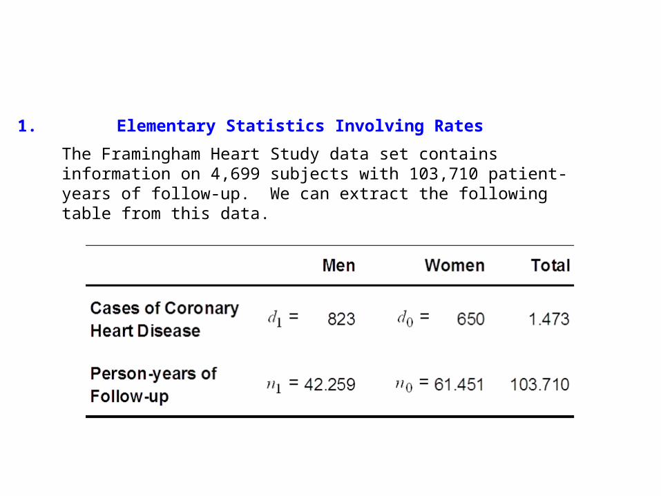
1. Elementary Statistics Involving Rates
The Framingham Heart Study data set contains information on 4,699 subjects with 103,710 patient-years of follow-up. We can extract the following table from this data.

a) Incidence
The incidence of CHD in men is
= 823/42,259
= 0.01948.
The incidence of CHD in women is
= 650/61,451
= 0.01058
d n1 1/
d n0 0/
b) Relative Risk
The relative risk of CHD in men compared to women is estimated by
= 0.01948/0.01058 = 1.841.1 1 0 0
ˆ ( / ) /( / )R d n d n
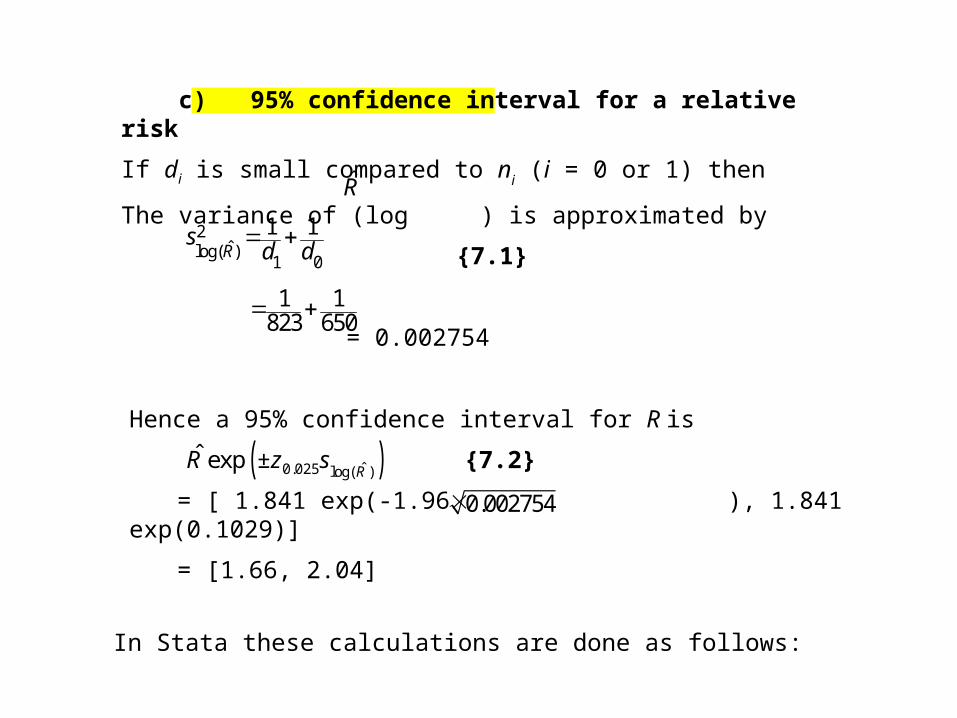
c) 95% confidence interval for a relative risk
If di is small compared to ni (i = 0 or 1) then
The variance of (log ) is approximated by
{7.1}
= 0.002754
R
2ˆlog( )
1 0
1 1R
sd d
1 1823 650
Hence a 95% confidence interval for R is
{7.2}
= [ 1.841 exp(-1.96 ), 1.841 exp(0.1029)]
= [1.66, 2.04]
( )ˆ0.025 log( )ˆexp
RR z s±
0.002754
In Stata these calculations are done as follows:
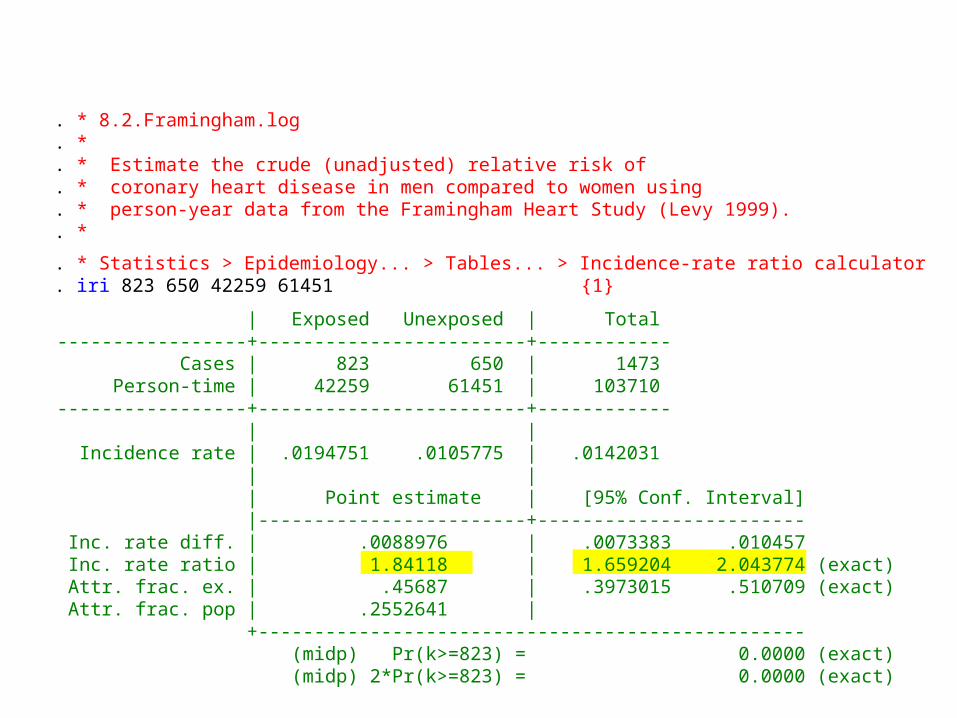
| Exposed Unexposed | Total-----------------+------------------------+------------ Cases | 823 650 | 1473 Person-time | 42259 61451 | 103710-----------------+------------------------+------------ | | Incidence rate | .0194751 .0105775 | .0142031 | | | Point estimate | [95% Conf. Interval] |------------------------+------------------------ Inc. rate diff. | .0088976 | .0073383 .010457 Inc. rate ratio | 1.84118 | 1.659204 2.043774 (exact) Attr. frac. ex. | .45687 | .3973015 .510709 (exact) Attr. frac. pop | .2552641 | +------------------------------------------------- (midp) Pr(k>=823) = 0.0000 (exact) (midp) 2*Pr(k>=823) = 0.0000 (exact)
. * 8.2.Framingham.log
. *
. * Estimate the crude (unadjusted) relative risk of
. * coronary heart disease in men compared to women using
. * person-year data from the Framingham Heart Study (Levy 1999).
. *
. * Statistics > Epidemiology... > Tables... > Incidence-rate ratio calculator
. iri 823 650 42259 61451 {1}
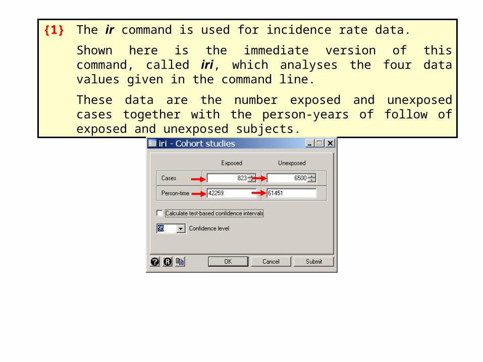
{1} The ir command is used for incidence rate data.
Shown here is the immediate version of this command, called iri, which analyses the four data values given in the command line.
These data are the number exposed and unexposed cases together with the person-years of follow of exposed and unexposed subjects.
. *
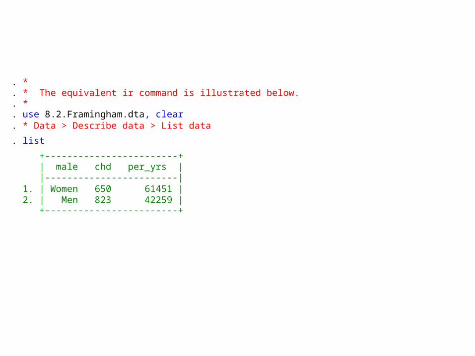
. * The equivalent ir command is illustrated below.
. *
. use 8.2.Framingham.dta, clear
. * Data > Describe data > List data
. list
+------------------------+ | male chd per_yrs | |------------------------| 1. | Women 650 61451 | 2. | Men 823 42259 | +------------------------+
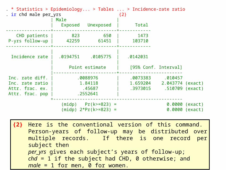
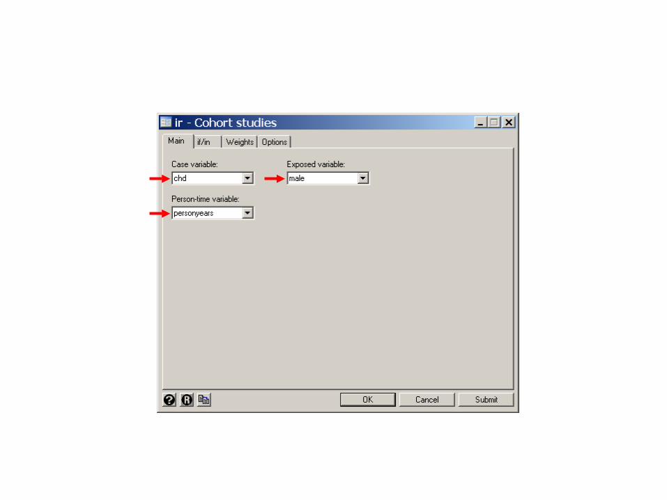
. * Statistics > Epidemiology... > Tables ... > Incidence-rate ratio
. ir chd male per_yrs {2} | Male | | Exposed Unexposed | Total-----------------+------------------------+------------ CHD patients | 823 650 | 1473 P-yrs follow-up | 42259 61451 | 103710-----------------+------------------------+------------ | | Incidence rate | .0194751 .0105775 | .0142031 | | | Point estimate | [95% Conf. Interval] |------------------------+------------------------ Inc. rate diff. | .0088976 | .0073383 .010457 Inc. rate ratio | 1.84118 | 1.659204 2.043774 (exact) Attr. frac. ex. | .45687 | .3973015 .510709 (exact) Attr. frac. pop | .2552641 | +------------------------------------------------- (midp) Pr(k>=823) = 0.0000 (exact) (midp) 2*Pr(k>=823) = 0.0000 (exact)
{2} Here is the conventional version of this command. Person-years of follow-up may be distributed over multiple records. If there is one record per subject thenper_yrs gives each subject’s years of follow-up; chd = 1 if the subject had CHD, 0 otherwise; and male = 1 for men, 0 for women.
We next introduce Poisson regression which is used for analyzing rates.
Poisson regression is used when the original data available to us is expressed as events per person-years of observation.
Poisson regression is also useful for analyzing data from large cohorts when the proportional hazards assumption is false. In this situation Poisson regression is quicker and easier to use than hazard regression with time-dependent covariates.
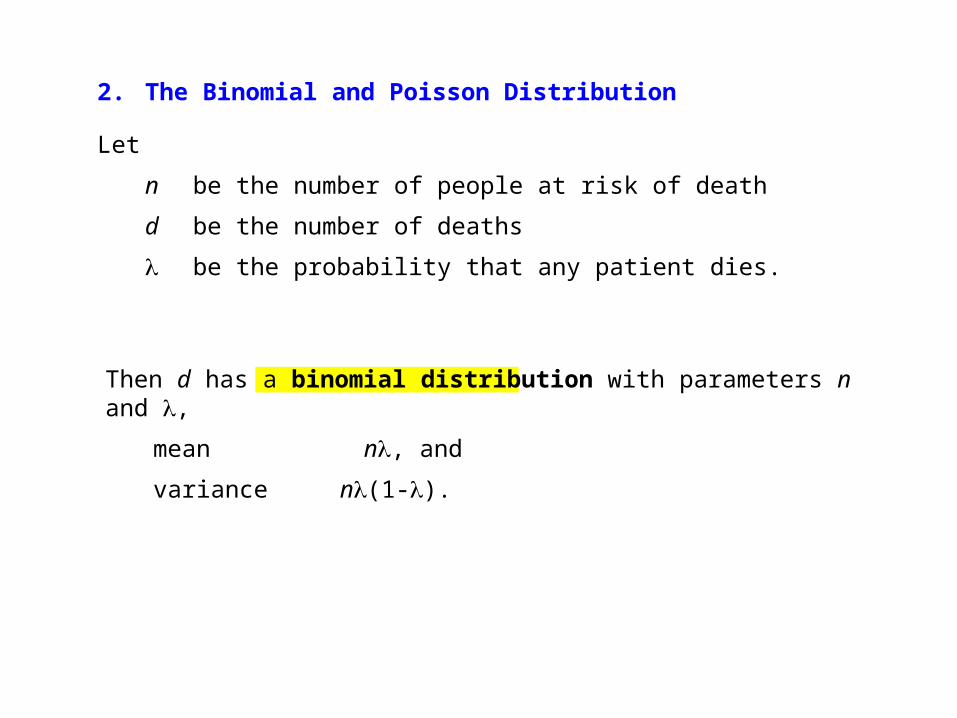
2. The Binomial and Poisson Distribution
Let
n be the number of people at risk of death
d be the number of deaths
be the probability that any patient dies.
Then d has a binomial distribution with parameters n and ,
mean n, and
variance n(1-).
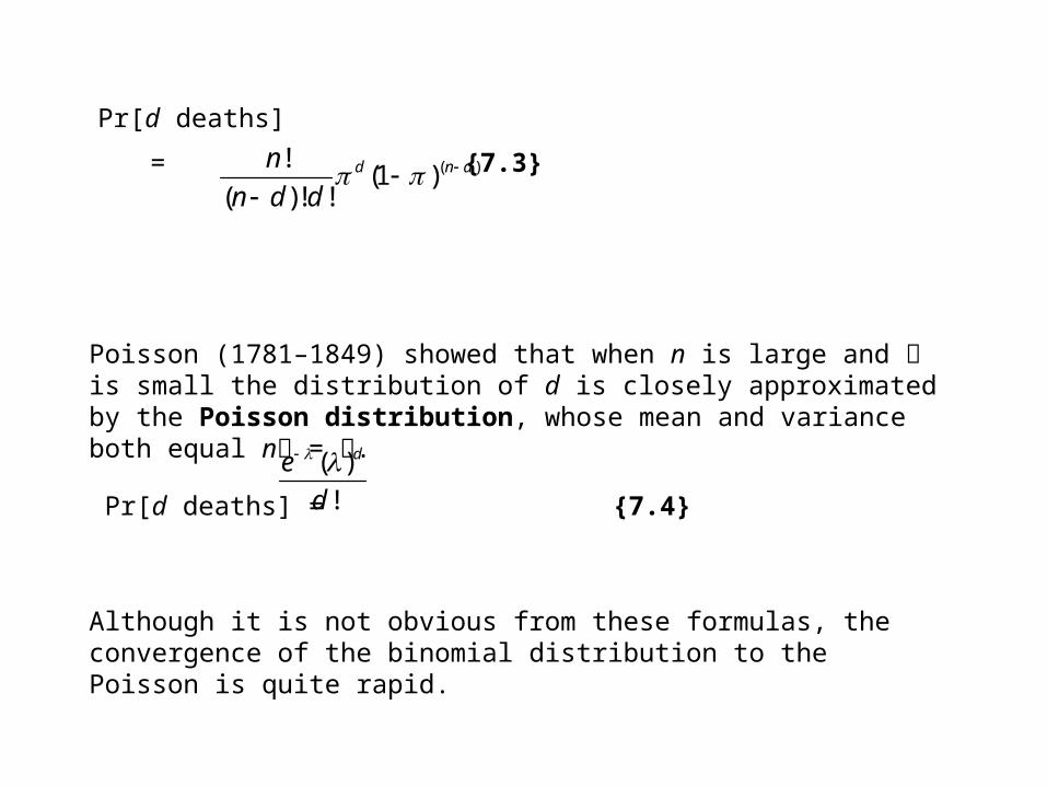
Pr[d deaths]
={7.3}
( )!(1 )
( )! !d n dn
n d d
Poisson (1781–1849) showed that when n is large and is small the distribution of d is closely approximated by the Poisson distribution, whose mean and variance both equal n = .
Pr[d deaths] = {7.4}
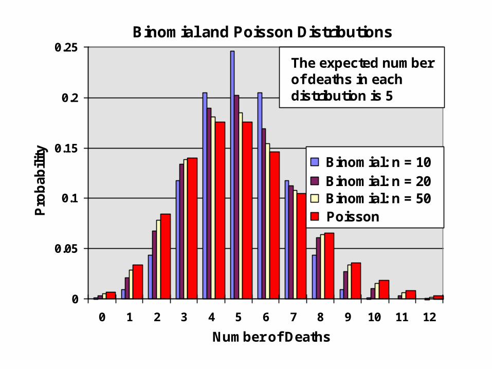
Although it is not obvious from these formulas, the convergence of the binomial distribution to the Poisson is quite rapid.
( )
!
de
d
0
0.05
0.1
0.15
0.2
0.25
0 1 2 3 4 5 6 7 8 9 10 11 12
Number of Deaths
Pro
bab
ility
Binomial: n = 10Binomial: n = 20Binomial: n = 50Poisson
Binomial and Poisson Distributions
The expected numberof deaths in each distribution is 5
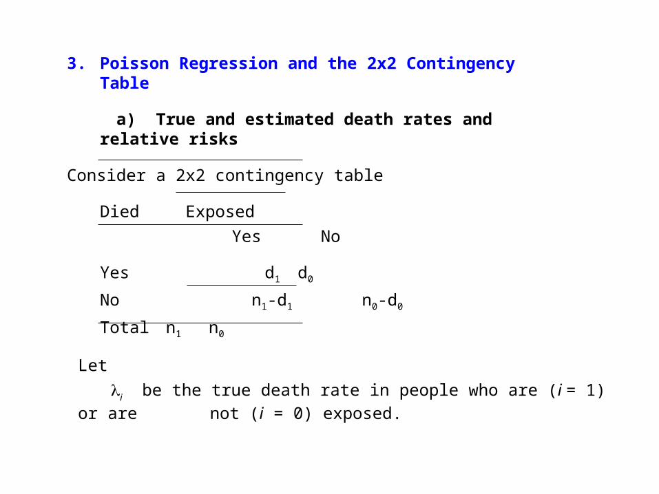
3. Poisson Regression and the 2x2 Contingency Table
a) True and estimated death rates and relative risks
Consider a 2x2 contingency table
Died Exposed
Yes No
Yes d1 d0
No n1-d1 n0-d0
Total n1 n0
Let
i be the true death rate in people who are (i = 1) or are not (i = 0) exposed.
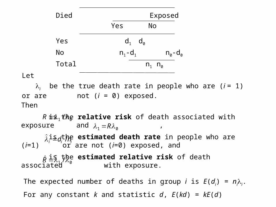
The expected number of deaths in group i is E(di) = nii.
For any constant k and statistic d, E(kd) = kE(d)
Died Exposed
Yes No
Yes d1 d0
No n1-d1 n0-d0
Total n1 n0
Let
i be the true death rate in people who are (i = 1) or are not (i = 0) exposed. Then
is the relative risk of death associated with exposure and ,
is the estimated death rate in people who are (i=1) or are not (i=0) exposed, and
is the estimated relative risk of death associated with exposure.
1 0RR 1 0/
/ i i id n
/ R 1 0
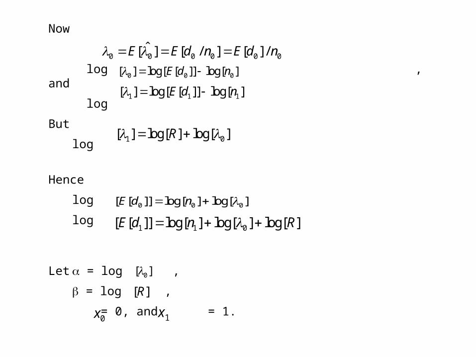
Now
log , and
log
But
log
0 0 0 0 0 0ˆ[ ] [ / ] [ ] /E E d n E d n
0 0 0[ ] log[ [ ]] log[ ]E d n
1 1 1[ ] log[ [ ]] log[ ]E d n
1 0[ ] log[ ] log[ ]R
Hence
log
log0 0 0[ [ ]] log[ ] log[ ]E d n
1 1 0[ [ ]] log[ ] log[ ] log[ ]E d n R
Let = log ,
= log ,
= 0, and = 1.
0[ ]
[ ]R
x0 1x
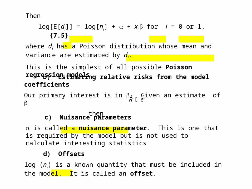
Then
log[E[di]] = log[ni] + + xi for i = 0 or 1, {7.5}
where di has a Poisson distribution whose mean and variance are estimated by di.
This is the simplest of all possible Poisson regression models. b) Estimating relative risks from the model coefficients
Our primary interest is in . Given an estimate of
then R e
c) Nuisance parameters
is called a nuisance parameter. This is one that is required by the model but is not used to calculate interesting statistics
d) Offsets
log (ni) is a known quantity that must be included in the model. It is called an offset.
4. Poisson Regression and Generalized Linear Models
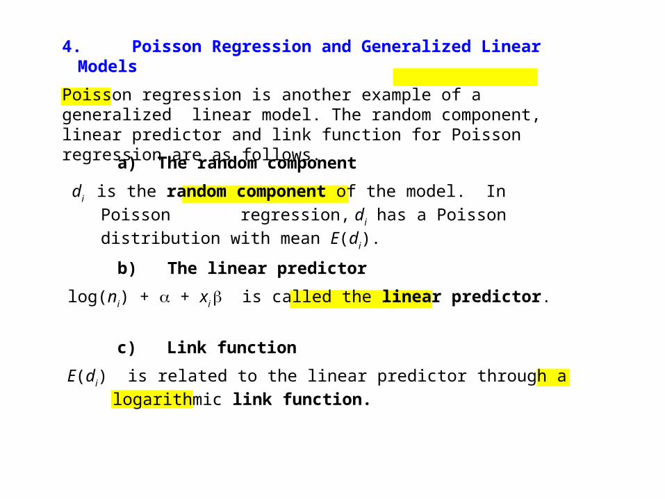
Poisson regression is another example of a generalized linear model. The random component, linear predictor and link function for Poisson regression are as follows.
a) The random component
di is the random component of the model. In Poisson regression, di has a Poisson distribution with mean E(di).
b) The linear predictor
log(ni) + + xi is called the linear predictor.
c) Link function
E(di) is related to the linear predictor through a logarithmic link function.
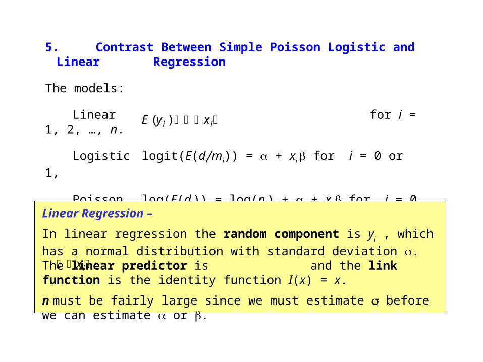
5. Contrast Between Simple Poisson Logistic and Linear Regression
The models:
Linear for i = 1, 2, …, n.
Logistic logit(E(di/mi)) = + xi for i = 0 or 1,
Poisson log(E(di)) = log(ni) + + xi for i = 0 or 1,
E y xi i( )
Linear Regression –
In linear regression the random component is yi , which has a normal distribution with standard deviation . The linear predictor is and the link function is the identity function I(x) = x.
n must be fairly large since we must estimate before we can estimate or .
xi

Logistic Regression –
In logistic regression we observe di events in mi trials. The random component is di, which has a binomial distribution. The linear predictor is . The model has a logit link function.
xi
Poisson Regression –
In Poisson regression we observe di events in ni trials. The random component is di, which has a Poisson distribution. The linear predictor is log(ni) + . The model has a logarithmic link function.
xi
In Poisson and logistic regression examples i has only 2 values. It is possible to estimate from these equations since we have reasonable estimates of the mean and variance of di for both of these models.
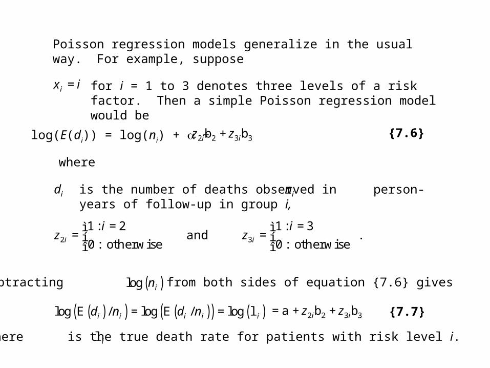
Poisson regression models generalize in the usual way. For example, suppose
ix i= for i = 1 to 3 denotes three levels of a risk factor. Then a simple Poisson regression model would be
log(E(di)) = log(ni) + + 2 2 3 3i iz zb + b
where
id is the number of deaths observed in person-years of follow-up in group i,
in
2
1: 2
0: otherwisei
iz
=ì=í
îand 3
1: 3
0: otherwisei
iz
=ì=í
î.
{7.6}
Subtracting from both sides of equation {7.6} gives( )log in
( )( ) ( )( ) ( )log E / log E / logi i i i id n d n= = l 2 2 3 3i iz z=a + b + b
where is the true death rate for patients with risk level i.il
{7.7}
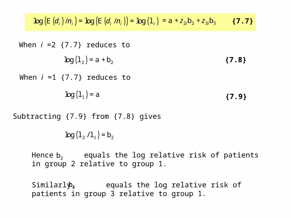
( )( ) ( )( ) ( )log E / log E / logi i i i id n d n= = l 2 2 3 3i iz z=a + b + b {7.7}
When i =2 {7.7} reduces to
( )2 2log l =a +b {7.8}
When i =1 {7.7} reduces to
( )1log l =a {7.9}
Subtracting {7.9} from {7.8} gives
( )2 1 2log /l l =b
Hence equals the log relative risk of patients in group 2 relative to group 1.
2b
Similarly, equals the log relative risk of patients in group 3 relative to group 1.
3b
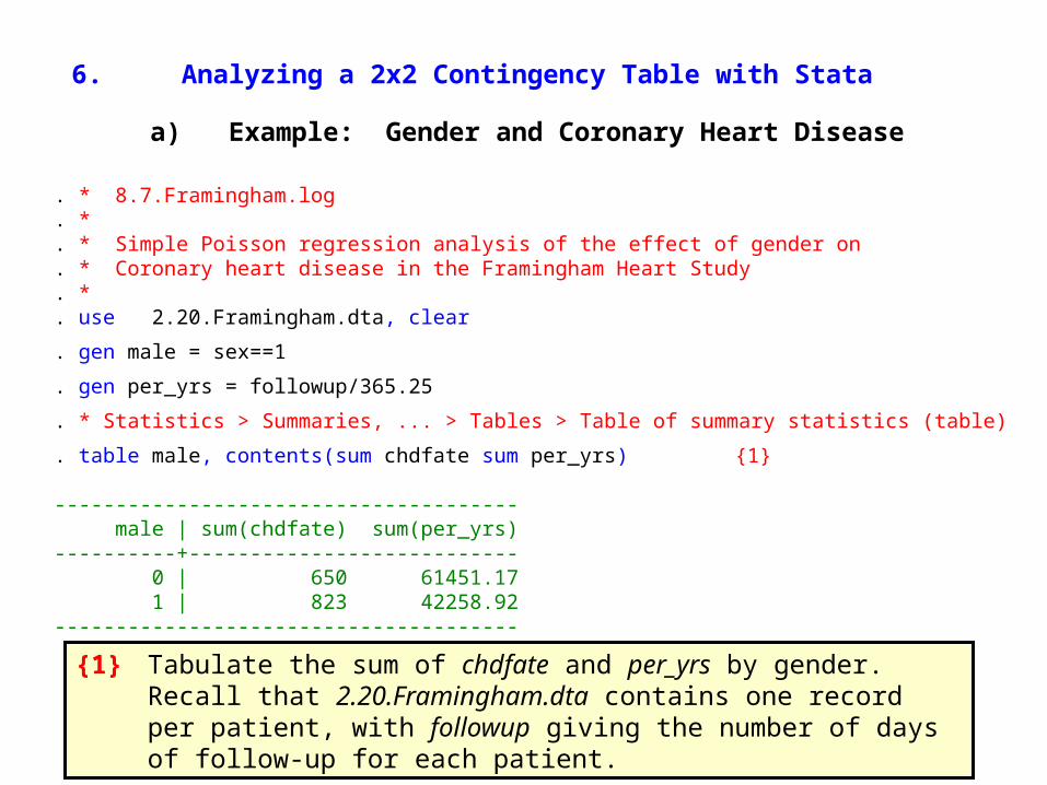
6. Analyzing a 2x2 Contingency Table with Stata
a) Example: Gender and Coronary Heart Disease
. * 8.7.Framingham.log
. *
. * Simple Poisson regression analysis of the effect of gender on
. * Coronary heart disease in the Framingham Heart Study
. *
. use 2.20.Framingham.dta, clear
. gen male = sex==1
. gen per_yrs = followup/365.25
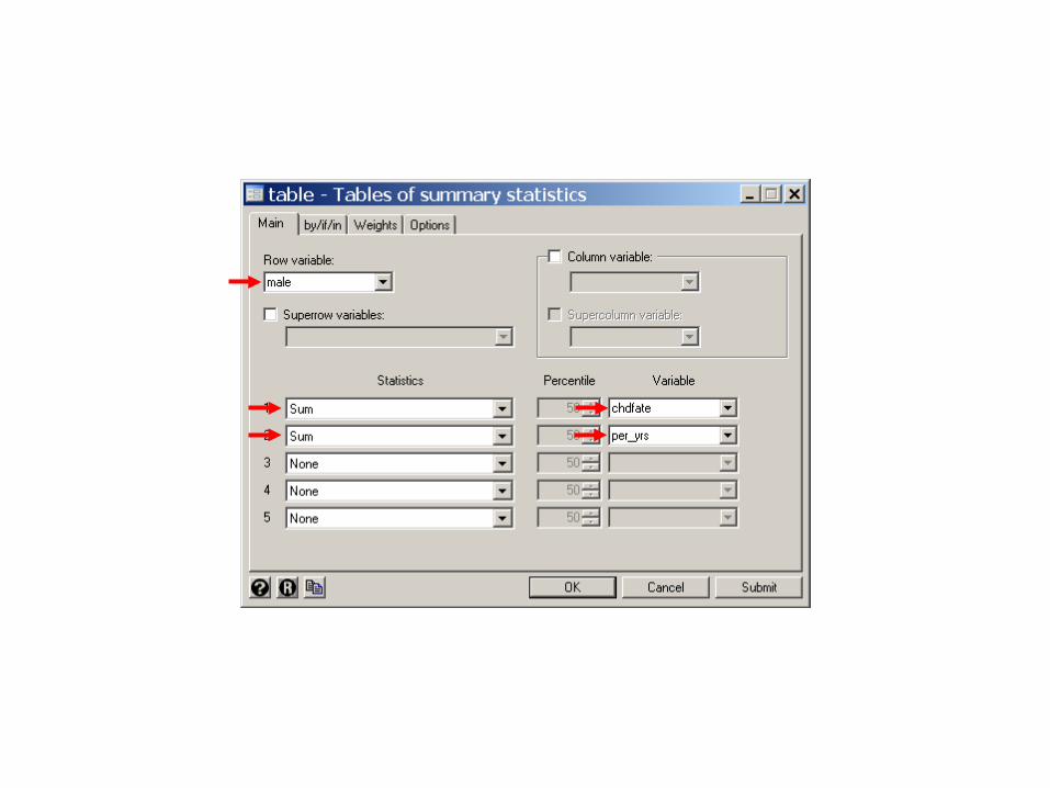
. * Statistics > Summaries, ... > Tables > Table of summary statistics (table)
. table male, contents(sum chdfate sum per_yrs) {1}
-------------------------------------- male | sum(chdfate) sum(per_yrs)----------+--------------------------- 0 | 650 61451.17 1 | 823 42258.92--------------------------------------
{1} Tabulate the sum of chdfate and per_yrs by gender. Recall that 2.20.Framingham.dta contains one record per patient, with followup giving the number of days of follow-up for each patient.
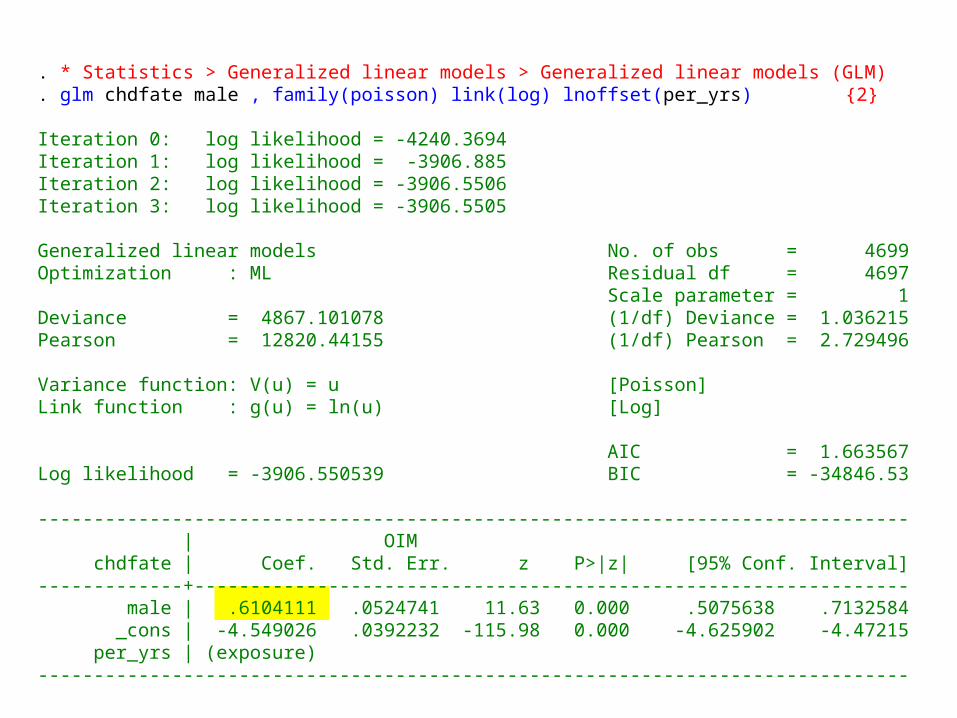
. * Statistics > Generalized linear models > Generalized linear models (GLM). glm chdfate male , family(poisson) link(log) lnoffset(per_yrs) {2} Iteration 0: log likelihood = -4240.3694 Iteration 1: log likelihood = -3906.885 Iteration 2: log likelihood = -3906.5506 Iteration 3: log likelihood = -3906.5505
Generalized linear models No. of obs = 4699Optimization : ML Residual df = 4697 Scale parameter = 1Deviance = 4867.101078 (1/df) Deviance = 1.036215Pearson = 12820.44155 (1/df) Pearson = 2.729496
Variance function: V(u) = u [Poisson]Link function : g(u) = ln(u) [Log]
AIC = 1.663567Log likelihood = -3906.550539 BIC = -34846.53
------------------------------------------------------------------------------ | OIM chdfate | Coef. Std. Err. z P>|z| [95% Conf. Interval]-------------+---------------------------------------------------------------- male | .6104111 .0524741 11.63 0.000 .5075638 .7132584 _cons | -4.549026 .0392232 -115.98 0.000 -4.625902 -4.47215 per_yrs | (exposure)------------------------------------------------------------------------------
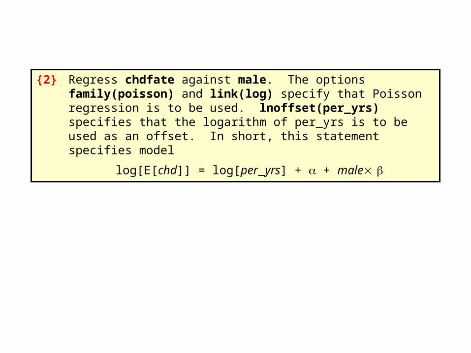
{2} Regress chdfate against male. The options family(poisson) and link(log) specify that Poisson regression is to be used. lnoffset(per_yrs) specifies that the logarithm of per_yrs is to be used as an offset. In short, this statement specifies model
log[E[chd]] = log[per_yrs] + + male

The exposure and lnoffset options are identical. They both enter the logarithm of per_yrs into the model as an offset.
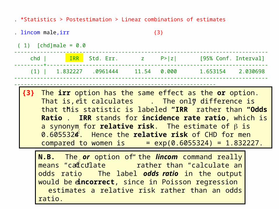
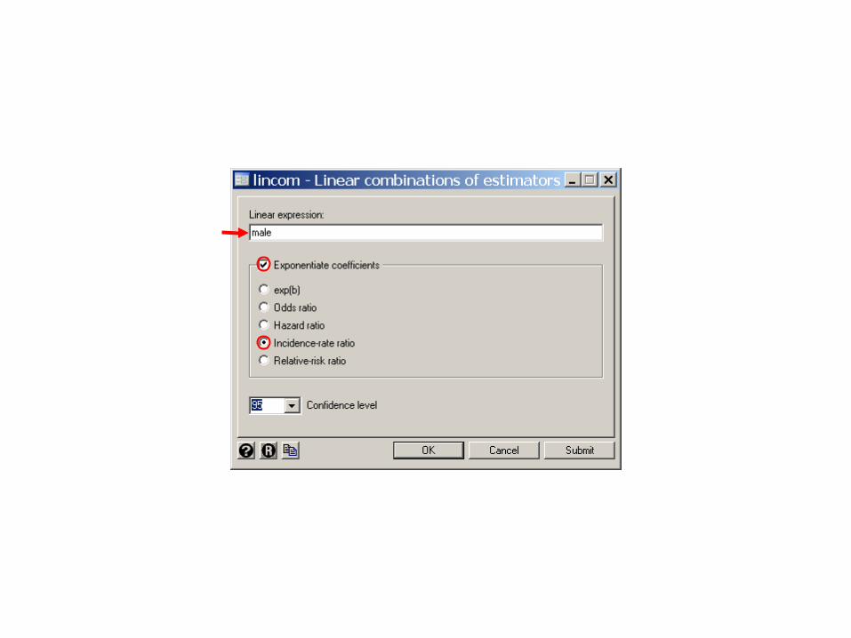
. *Statistics > Postestimation > Linear combinations of estimates . lincom male,irr {3} ( 1) [chd]male = 0.0 ------------------------------------------------------------------------------ chd | IRR Std. Err. z P>|z| [95% Conf. Interval]---------+-------------------------------------------------------------------- (1) | 1.832227 .0961444 11.54 0.000 1.653154 2.030698--------------------------------------------------------------------------------------------------------------------------------------------
N.B. The or option of the lincom command really means “calculate ” rather than “calculate an odds ratio” The label odds ratio in the output would be incorrect, since in Poisson regression estimates a relative risk rather than an odds ratio.
e
e
{3} The irr option has the same effect as the or option. That is, it calculates . The only difference is that this statistic is labeled “IRR” rather than “Odds Ratio”. IRR stands for incidence rate ratio, which is a synonym for relative risk. The estimate of is 0.6055324. Hence the relative risk of CHD for men compared to women is = exp(0.6055324) = 1.832227. e
e
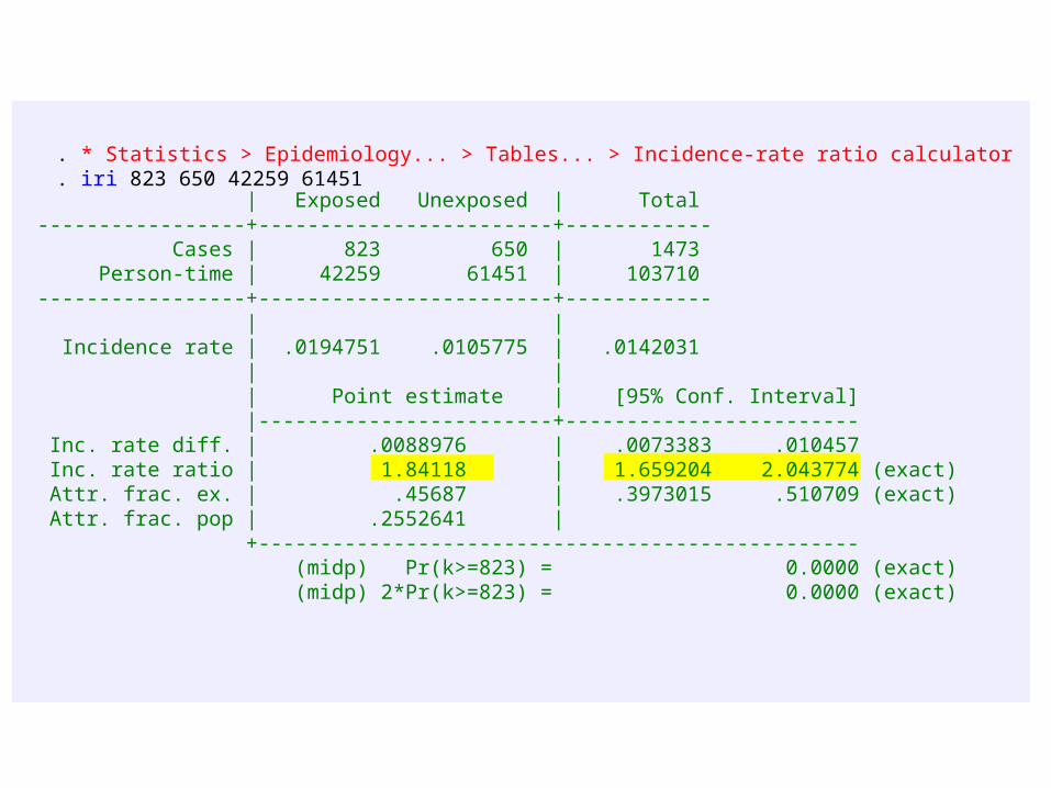
. * Statistics > Epidemiology... > Tables... > Incidence-rate ratio calculator
. iri 823 650 42259 61451 | Exposed Unexposed | Total-----------------+------------------------+------------ Cases | 823 650 | 1473 Person-time | 42259 61451 | 103710-----------------+------------------------+------------ | | Incidence rate | .0194751 .0105775 | .0142031 | | | Point estimate | [95% Conf. Interval] |------------------------+------------------------ Inc. rate diff. | .0088976 | .0073383 .010457 Inc. rate ratio | 1.84118 | 1.659204 2.043774 (exact) Attr. frac. ex. | .45687 | .3973015 .510709 (exact) Attr. frac. pop | .2552641 | +------------------------------------------------- (midp) Pr(k>=823) = 0.0000 (exact) (midp) 2*Pr(k>=823) = 0.0000 (exact)
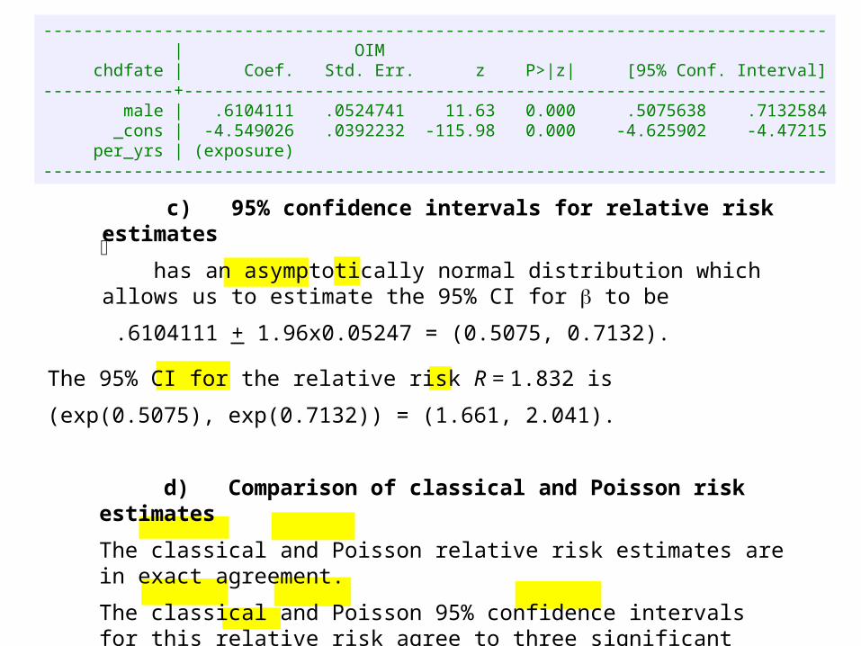
c) 95% confidence intervals for relative risk estimates
has an asymptotically normal distribution which allows us to estimate the 95% CI for to be
.6104111 + 1.96x0.05247 = (0.5075, 0.7132).
d) Comparison of classical and Poisson risk estimates
The classical and Poisson relative risk estimates are in exact agreement.
The classical and Poisson 95% confidence intervals for this relative risk agree to three significant figures.
The 95% CI for the relative risk R = 1.832 is
(exp(0.5075), exp(0.7132)) = (1.661, 2.041).
------------------------------------------------------------------------------ | OIM chdfate | Coef. Std. Err. z P>|z| [95% Conf. Interval]-------------+---------------------------------------------------------------- male | .6104111 .0524741 11.63 0.000 .5075638 .7132584 _cons | -4.549026 .0392232 -115.98 0.000 -4.625902 -4.47215 per_yrs | (exposure)------------------------------------------------------------------------------

Testing the null hypothesis that R = 1 is equivalent to testing the null hypothesis that = 0.
The P value associated with this test is < 0.0005.
. lincom male,irr ( 1) [chdfate]male = 0
------------------------------------------------------------------------------ chdfate | IRR Std. Err. z P>|z| [95% Conf. Interval]-------------+---------------------------------------------------------------- (1) | 1.841188 .0966146 11.63 0.000 1.661239 2.04063------------------------------------------------------------------------------
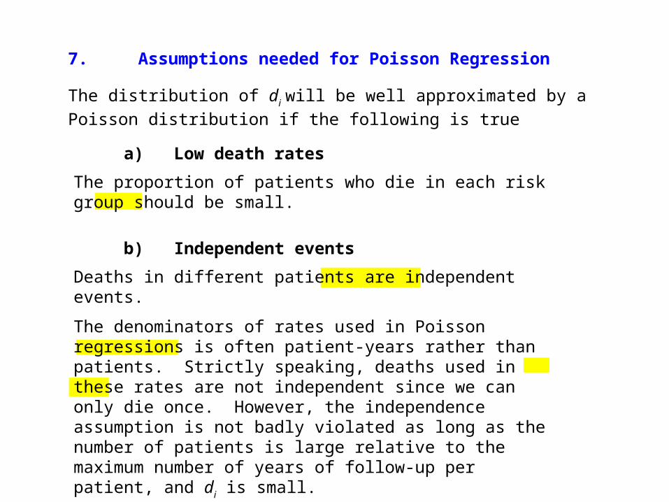
7. Assumptions needed for Poisson Regression
The distribution of di will be well approximated by a Poisson distribution if the following is true
a) Low death rates
The proportion of patients who die in each risk group should be small.
b) Independent events
Deaths in different patients are independent events.
The denominators of rates used in Poisson regressions is often patient-years rather than patients. Strictly speaking, deaths used in these rates are not independent since we can only die once. However, the independence assumption is not badly violated as long as the number of patients is large relative to the maximum number of years of follow-up per patient, and di is small.
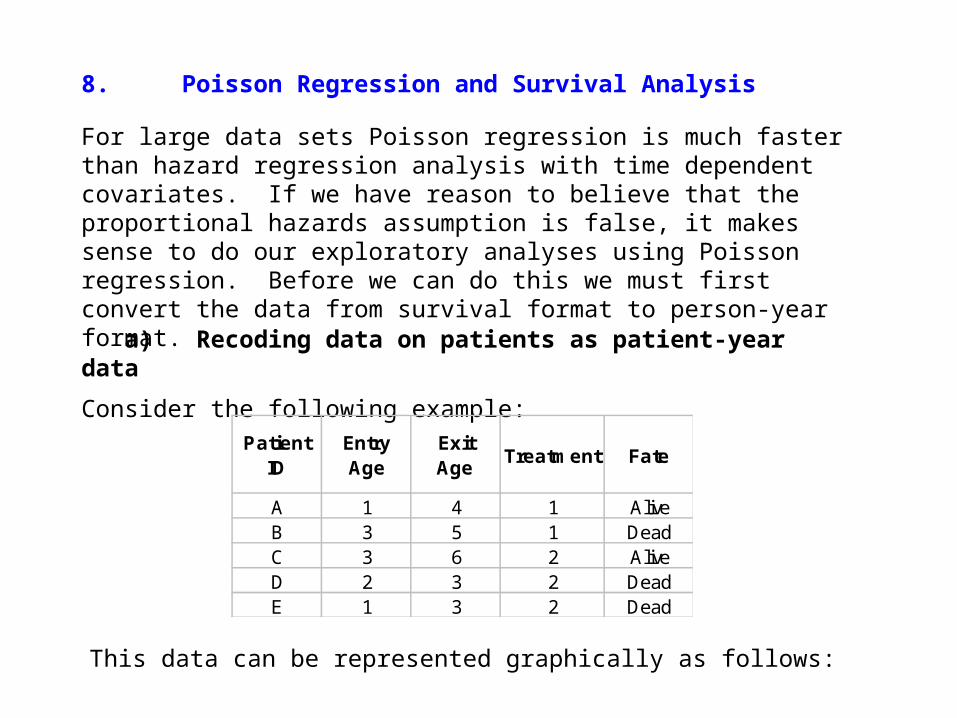
8. Poisson Regression and Survival Analysis
For large data sets Poisson regression is much faster than hazard regression analysis with time dependent covariates. If we have reason to believe that the proportional hazards assumption is false, it makes sense to do our exploratory analyses using Poisson regression. Before we can do this we must first convert the data from survival format to person-year format.
a) Recoding data on patients as patient-year data
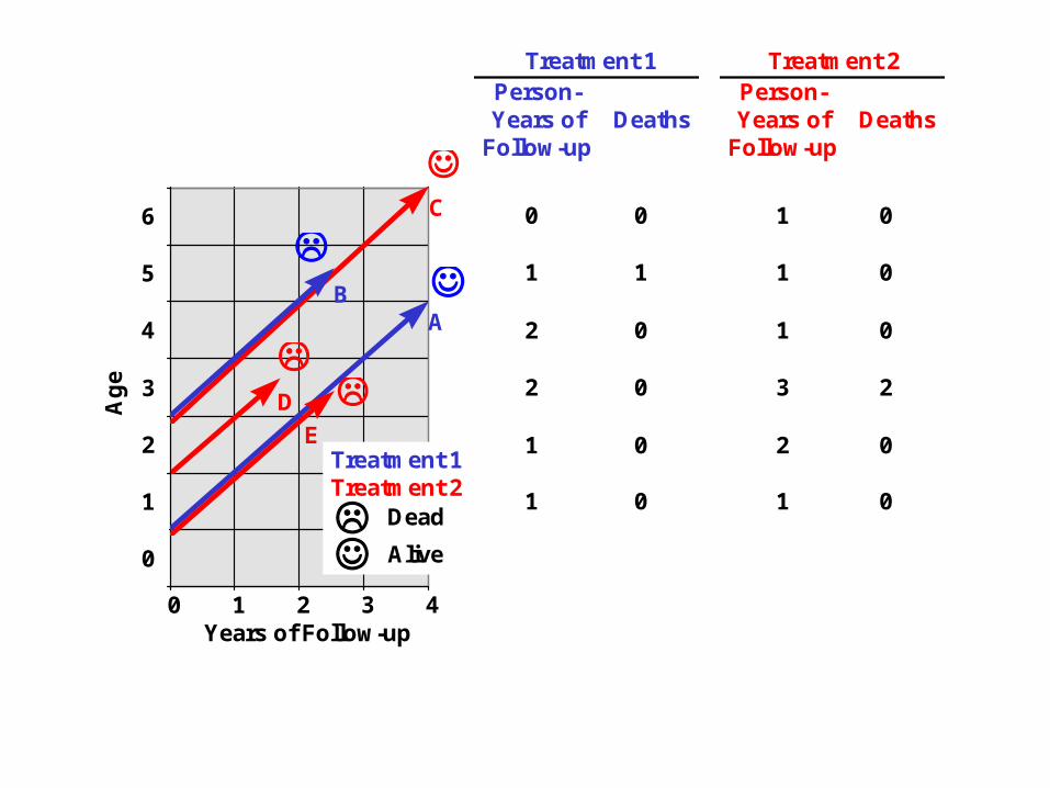
Consider the following example:
Patient ID
Entry Age
Exit Age
Treatment Fate
A 1 4 1 AliveB 3 5 1 DeadC 3 6 2 AliveD 2 3 2 DeadE 1 3 2 Dead
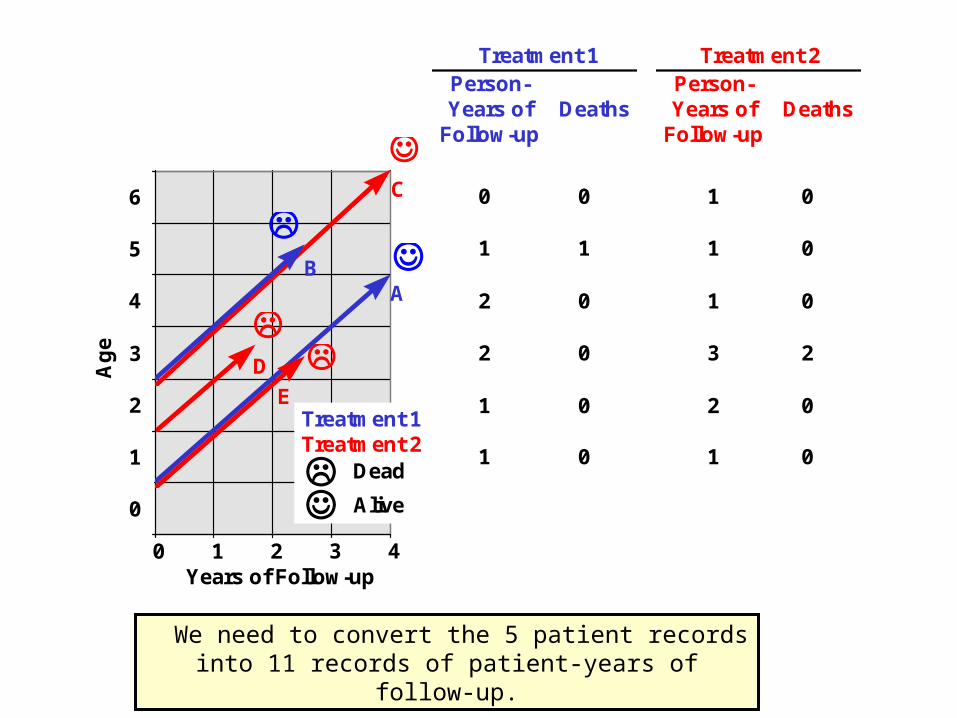
This data can be represented graphically as follows:
Ag
e
Years of Follow-up
0
1
2
3
4
5
6
0 1 2 3 4
AB
C
D
E
Treatment 1Treatment 2
Dead
Alive
Treatment 1Person-Years of
Follow-upDeaths
Treatment 2Person-Years of
Follow-upDeaths
0 0 1 0
1 1 1 0
2 0 1 0
2 0 3 2
1 0 2 0
1 0 1 0
We need to convert the 5 patient records into 11 records of patient-years of follow-up.
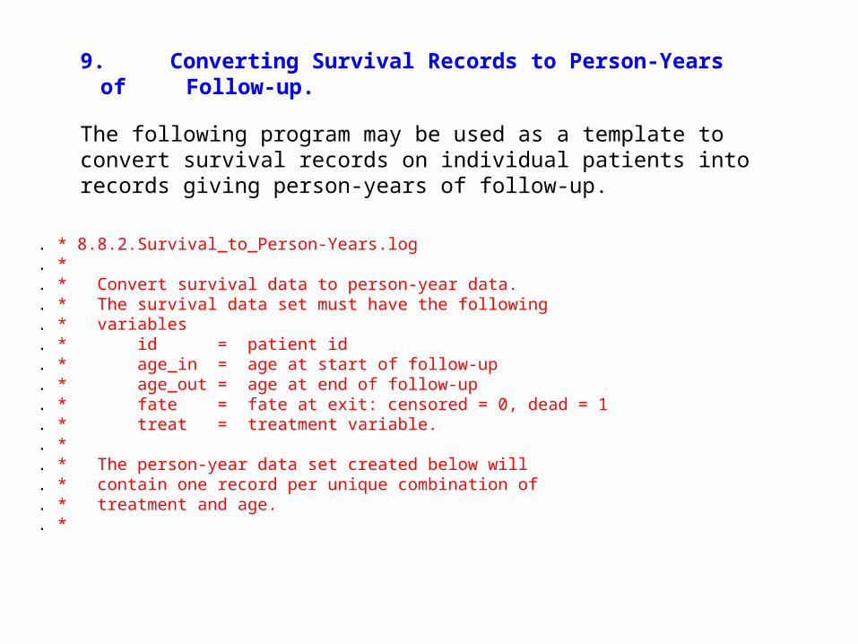
9. Converting Survival Records to Person-Years of Follow-up.
The following program may be used as a template to convert survival records on individual patients into records giving person-years of follow-up.
. * 8.8.2.Survival_to_Person-Years.log
. *
. * Convert survival data to person-year data.
. * The survival data set must have the following
. * variables
. * id = patient id
. * age_in = age at start of follow-up
. * age_out = age at end of follow-up
. * fate = fate at exit: censored = 0, dead = 1
. * treat = treatment variable.
. *
. * The person-year data set created below will
. * contain one record per unique combination of
. * treatment and age.
. *
. * Variables in the person-year data set that must not
. * be in the original survival data set are
. * age_now = an age of people in the cohort
. * pt_yrs = number of patient-years of observations
. * of people receiving therapy treat who
. * are age_now years old.
. * deaths = number of events (fate=1) occurring in
. * pt_yrs years of follow-up for this
. * group of patients.
. *
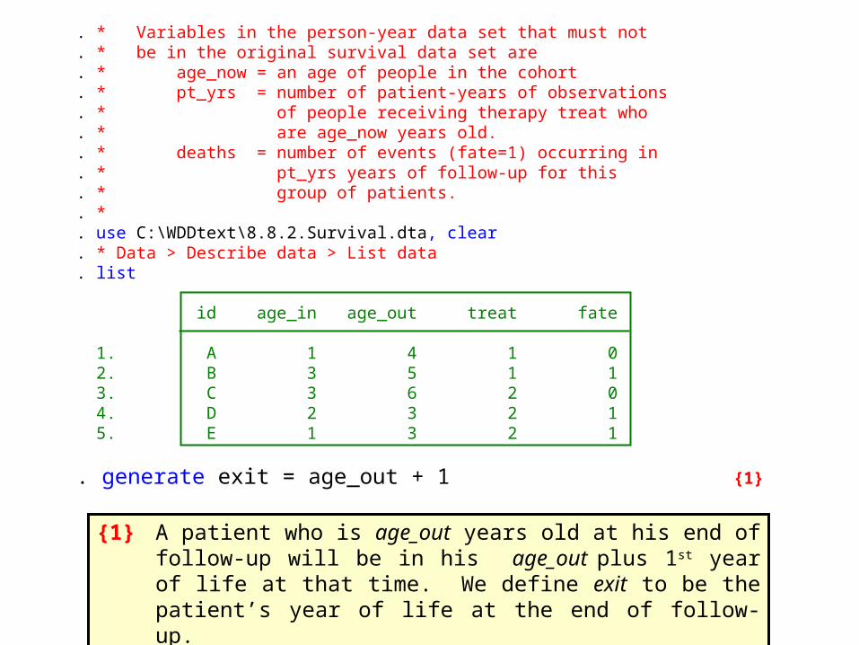
. use C:\WDDtext\8.8.2.Survival.dta, clear
. * Data > Describe data > List data
. list
id age_in age_out treat fate 1. A 1 4 1 0 2. B 3 5 1 1 3. C 3 6 2 0 4. D 2 3 2 1 5. E 1 3 2 1
. generate exit = age_out + 1 {1}
{1} A patient who is age_out years old at his end of follow-up will be in his age_out plus 1st year of life at that time. We define exit to be the patient’s year of life at the end of follow-up.
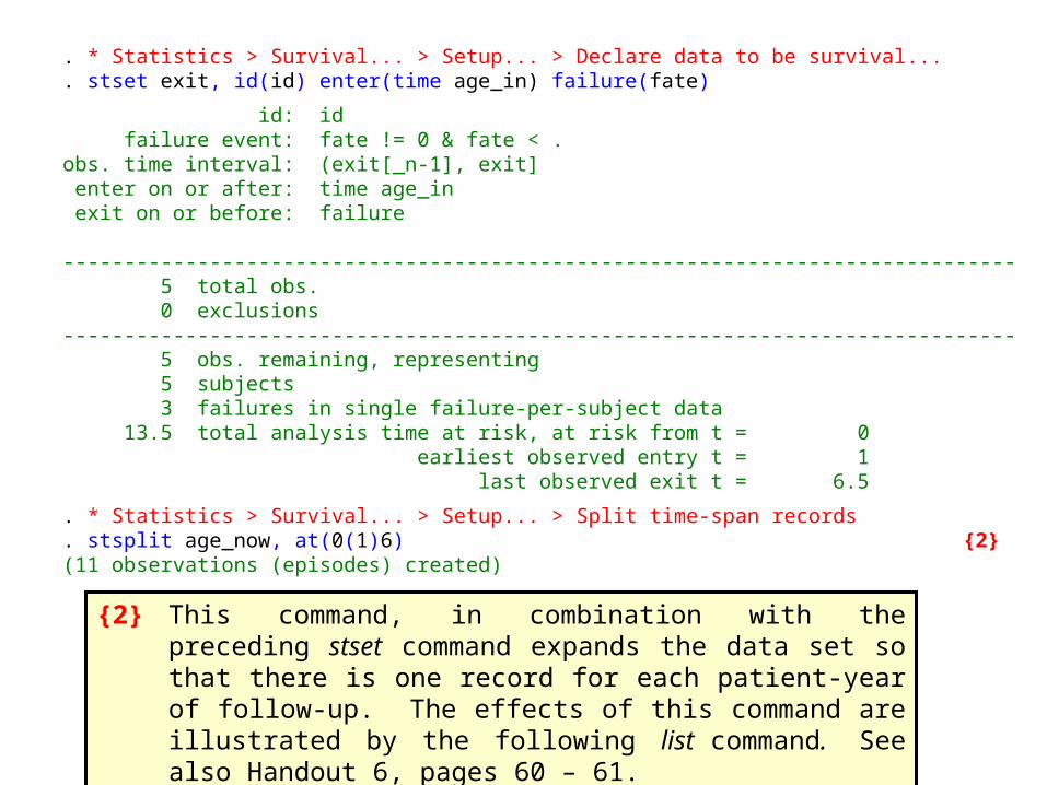
. * Statistics > Survival... > Setup... > Declare data to be survival...
. stset exit, id(id) enter(time age_in) failure(fate)
id: id failure event: fate != 0 & fate < .obs. time interval: (exit[_n-1], exit] enter on or after: time age_in exit on or before: failure
------------------------------------------------------------------------------ 5 total obs. 0 exclusions------------------------------------------------------------------------------ 5 obs. remaining, representing 5 subjects 3 failures in single failure-per-subject data 13.5 total analysis time at risk, at risk from t = 0 earliest observed entry t = 1 last observed exit t = 6.5
. * Statistics > Survival... > Setup... > Split time-span records
. stsplit age_now, at(0(1)6) {2}(11 observations (episodes) created)
{2} This command, in combination with the preceding stset command expands the data set so that there is one record for each patient-year of follow-up. The effects of this command are illustrated by the following list command. See also Handout 6, pages 60 – 61.
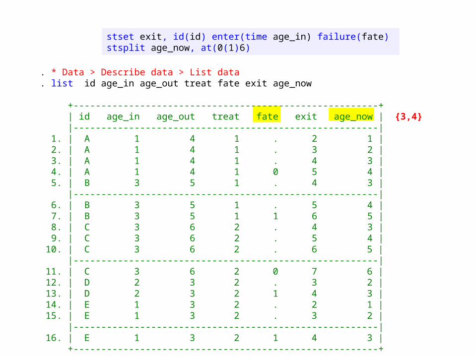
. * Data > Describe data > List data
. list id age_in age_out treat fate exit age_now
+-------------------------------------------------------+ | id age_in age_out treat fate exit age_now | {3,4} |-------------------------------------------------------| 1. | A 1 4 1 . 2 1 | 2. | A 1 4 1 . 3 2 | 3. | A 1 4 1 . 4 3 | 4. | A 1 4 1 0 5 4 | 5. | B 3 5 1 . 4 3 | |-------------------------------------------------------| 6. | B 3 5 1 . 5 4 | 7. | B 3 5 1 1 6 5 | 8. | C 3 6 2 . 4 3 | 9. | C 3 6 2 . 5 4 | 10. | C 3 6 2 . 6 5 | |-------------------------------------------------------| 11. | C 3 6 2 0 7 6 | 12. | D 2 3 2 . 3 2 | 13. | D 2 3 2 1 4 3 | 14. | E 1 3 2 . 2 1 | 15. | E 1 3 2 . 3 2 | |-------------------------------------------------------| 16. | E 1 3 2 1 4 3 | +-------------------------------------------------------+
stset exit, id(id) enter(time age_in) failure(fate) stsplit age_now, at(0(1)6)
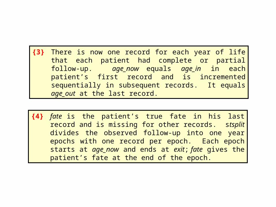
{4} fate is the patient’s true fate in his last record and is missing for other records. stsplit divides the observed follow-up into one year epochs with one record per epoch. Each epoch starts at age_now and ends at exit; fate gives the patient’s fate at the end of the epoch.
{3} There is now one record for each year of life that each patient had complete or partial follow-up. age_now equals age_in in each patient’s first record and is incremented sequentially in subsequent records. It equals age_out at the last record.

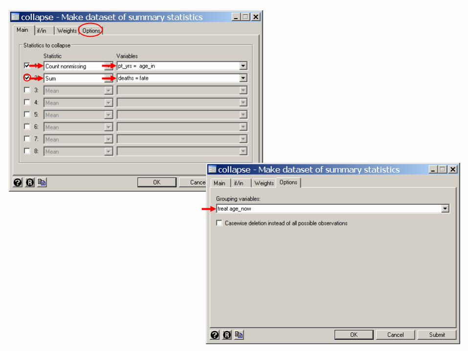
. sort treat age_now
. * Data > Create... > Other variable-trans... > Make dataset of means...
. collapse (count) pt_yrs=age_in (sum) deaths=fate, by(treat age_now) {5}
{5} This statement collapses all records with identical values of treat and age_now into a single record. pt_yrs is set equal to the number of records collapsed. (More precisely, it is the count of collapsed records with non-missing values of age_in.)
deaths is set equal to the number of deaths (the sum of non-missing values of fate over these records). All variables are deleted from memory except treat age_now pt_yrs and deaths.
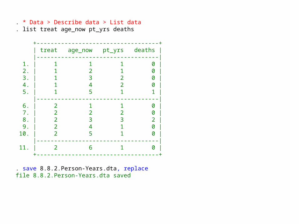
. * Data > Describe data > List data
. list treat age_now pt_yrs deaths
+-----------------------------------+ | treat age_now pt_yrs deaths | |-----------------------------------| 1. | 1 1 1 0 | 2. | 1 2 1 0 | 3. | 1 3 2 0 | 4. | 1 4 2 0 | 5. | 1 5 1 1 | |-----------------------------------| 6. | 2 1 1 0 | 7. | 2 2 2 0 | 8. | 2 3 3 2 | 9. | 2 4 1 0 | 10. | 2 5 1 0 | |-----------------------------------| 11. | 2 6 1 0 | +-----------------------------------+
. save 8.8.2.Person-Years.dta, replacefile 8.8.2.Person-Years.dta saved
Ag
e
Years of Follow-up
0
1
2
3
4
5
6
0 1 2 3 4
AB
C
D
E
Treatment 1Treatment 2
Dead
Alive
Treatment 1Person-Years of
Follow-upDeaths
Treatment 2Person-Years of
Follow-upDeaths
0 0 1 0
1 1 1 0
2 0 1 0
2 0 3 2
1 0 2 0
1 0 1 0
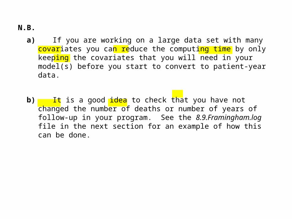
N.B.
a) If you are working on a large data set with many covariates you can reduce the computing time by only keeping the covariates that you will need in your model(s) before you start to convert to patient-year data.
b) It is a good idea to check that you have not changed the number of deaths or number of years of follow-up in your program. See the 8.9.Framingham.log file in the next section for an example of how this can be done.
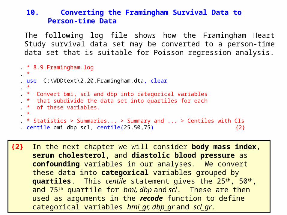
10. Converting the Framingham Survival Data to Person-time Data
The following log file shows how the Framingham Heart Study survival data set may be converted to a person-time data set that is suitable for Poisson regression analysis.
. * 8.9.Framingham.log
. *
. use C:\WDDtext\2.20.Framingham.dta, clear
. *
. * Convert bmi, scl and dbp into categorical variables
. * that subdivide the data set into quartiles for each
. * of these variables.
. *
. * Statistics > Summaries... > Summary and ... > Centiles with CIs
. centile bmi dbp scl, centile(25,50,75) {2}
{2} In the next chapter we will consider body mass index, serum cholesterol, and diastolic blood pressure as confounding variables in our analyses. We convert these data into categorical variables grouped by quartiles. This centile statement gives the 25th, 50th, and 75th quartile for bmi, dbp and scl. These are then used as arguments in the recode function to define categorical variables bmi_gr, dbp_gr and scl_gr.

-- Binom. Interp. --Variable | Obs Percentile Centile [95% Conf. Interval]---------+----------------------------------------------------------- bmi | 4690 25 22.8 22.7 23 | 50 25.2 25.1 25.36161 | 75 28 27.9 28.1 dbp | 4699 25 74 74 74 | 50 80 80 82 | 75 90 90 90 scl | 4666 25 197 196 199 | 50 225 222 225 | 75 255 252 256
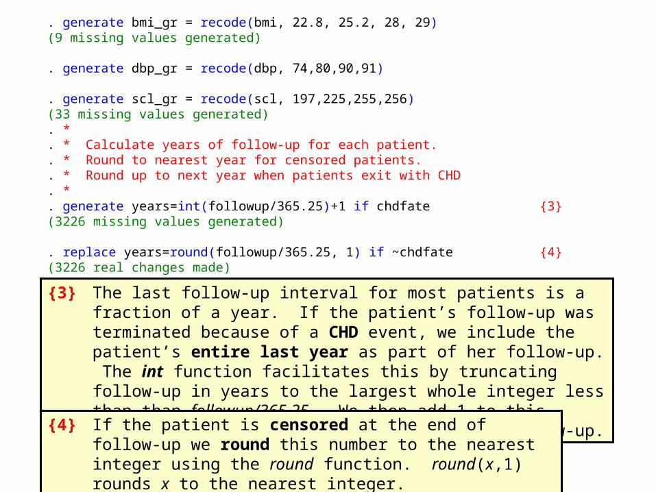
. generate bmi_gr = recode(bmi, 22.8, 25.2, 28, 29)(9 missing values generated) . generate dbp_gr = recode(dbp, 74,80,90,91) . generate scl_gr = recode(scl, 197,225,255,256)(33 missing values generated). *. * Calculate years of follow-up for each patient.. * Round to nearest year for censored patients.. * Round up to next year when patients exit with CHD. *. generate years=int(followup/365.25)+1 if chdfate {3}(3226 missing values generated) . replace years=round(followup/365.25, 1) if ~chdfate {4}(3226 real changes made)
{3} The last follow-up interval for most patients is a fraction of a year. If the patient’s follow-up was terminated because of a CHD event, we include the patient’s entire last year as part of her follow-up. The int function facilitates this by truncating follow-up in years to the largest whole integer less than than followup/365.25. We then add 1 to this number to include the entire last year of follow-up.
{4} If the patient is censored at the end of follow-up we round this number to the nearest integer using the round function. round(x,1) rounds x to the nearest integer.

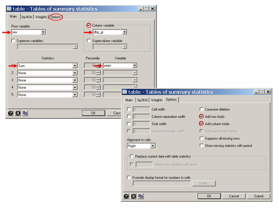
. * Statistics > Summaries... > Tables > Table of summary statistics (table).
. table sex dbp_gr, contents(sum years) row col {5} ----------+--------------------------------------- | dbp_gr Sex | 74 80 90 91 Total----------+--------------------------------------- Men | 10663 10405 12795 8825 42688 {6} Women | 21176 14680 15348 10569 61773 | Total | 31839 25085 28143 19394 104461----------+---------------------------------------
{5} So far, we haven’t added any records or modified any of the original variables. Before doing this it is a good idea to tabulate the number of person-years of follow-up and CHD events in the data set. At the end of the transformation we can recalculate these tables to ensure that we have not lost or added any spurious years of follow-up or CHD events.
The next two tables show these data cross tabulated by sex and dbp_gr. The contents(sum years) option causes years to be summed over every unique combination of values of sex and dbp_gr and displayed in the table. {6} For example, the sum of the years variable for men with dbp_gr = 90 is 12,795. This means that there are 12,795 person-years of follow-up for men with baseline diastolic blood pressures between 80 and 90.
. * Statistics > Summaries... > Tables > Table of summary statistics (table).
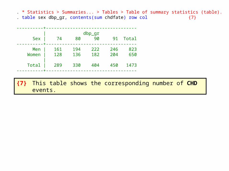
. table sex dbp_gr, contents(sum chdfate) row col {7} ----------+---------------------------------- | dbp_gr Sex | 74 80 90 91 Total----------+---------------------------------- Men | 161 194 222 246 823 Women | 128 136 182 204 650 | Total | 289 330 404 450 1473----------+----------------------------------
{7} This table shows the corresponding number of CHD events.
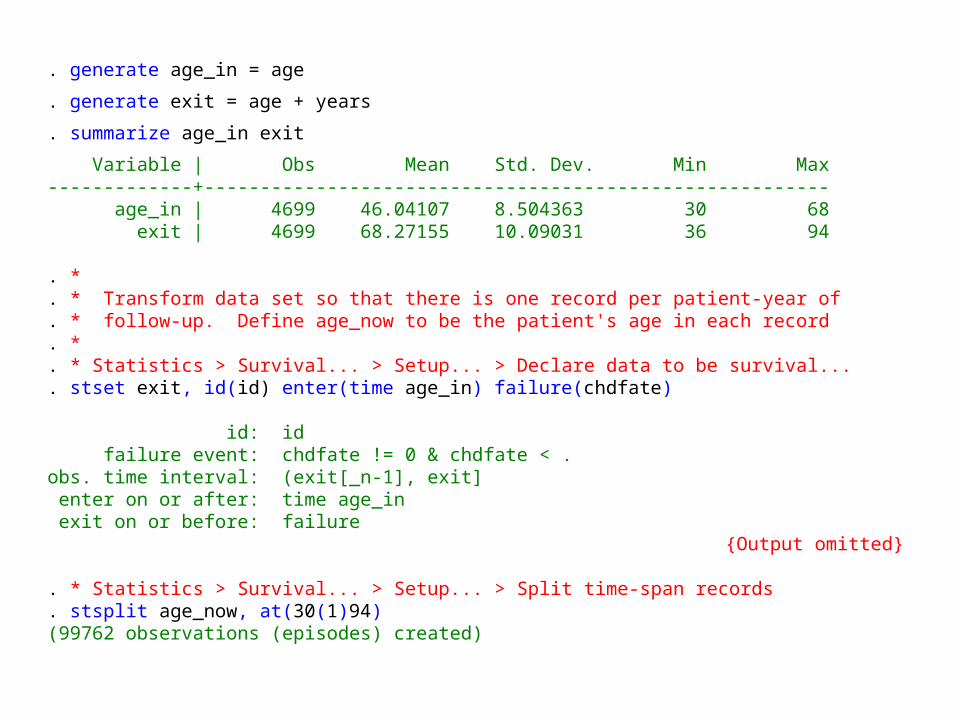
. generate age_in = age
. generate exit = age + years
. summarize age_in exit
Variable | Obs Mean Std. Dev. Min Max-------------+-------------------------------------------------------- age_in | 4699 46.04107 8.504363 30 68 exit | 4699 68.27155 10.09031 36 94 . *. * Transform data set so that there is one record per patient-year of . * follow-up. Define age_now to be the patient's age in each record. *. * Statistics > Survival... > Setup... > Declare data to be survival.... stset exit, id(id) enter(time age_in) failure(chdfate)
id: id failure event: chdfate != 0 & chdfate < .obs. time interval: (exit[_n-1], exit] enter on or after: time age_in exit on or before: failure
{Output omitted}
. * Statistics > Survival... > Setup... > Split time-span records
. stsplit age_now, at(30(1)94)(99762 observations (episodes) created)
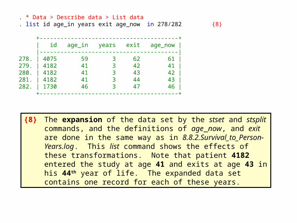
{8} The expansion of the data set by the stset and stsplit commands, and the definitions of age_now, and exit are done in the same way as in 8.8.2.Survival_to_Person-Years.log. This list command shows the effects of these transformations. Note that patient 4182 entered the study at age 41 and exits at age 43 in his 44th year of life. The expanded data set contains one record for each of these years.
. * Data > Describe data > List data
. list id age_in years exit age_now in 278/282 {8}
+----------------------------------------+ | id age_in years exit age_now | |----------------------------------------|278. | 4075 59 3 62 61 |279. | 4182 41 3 42 41 |280. | 4182 41 3 43 42 |281. | 4182 41 3 44 43 |282. | 1730 46 3 47 46 | +----------------------------------------+
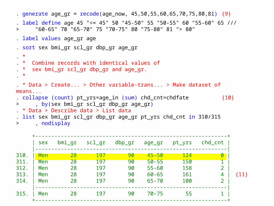
. generate age_gr = recode(age_now, 45,50,55,60,65,70,75,80,81) {9}
. label define age 45 "<= 45" 50 "45-50" 55 "50-55" 60 "55-60" 65 ///> "60-65" 70 "65-70" 75 "70-75" 80 "75-80" 81 "> 80"
. label values age_gr age
. sort sex bmi_gr scl_gr dbp_gr age_gr
. *
. * Combine records with identical values of
. * sex bmi_gr scl_gr dbp_gr and age_gr.
. *
. * Data > Create... > Other variable-trans... > Make dataset of means.... collapse (count) pt_yrs=age_in (sum) chd_cnt=chdfate {10} > , by(sex bmi_gr scl_gr dbp_gr age_gr). * Data > Describe data > List data. list sex bmi_gr scl_gr dbp_gr age_gr pt_yrs chd_cnt in 310/315 > , nodisplay
+------------------------------------------------------------+ | sex bmi_gr scl_gr dbp_gr age_gr pt_yrs chd_cnt | |------------------------------------------------------------|310. | Men 28 197 90 45-50 124 0 |311. | Men 28 197 90 50-55 150 1 |312. | Men 28 197 90 55-60 158 2 |313. | Men 28 197 90 60-65 161 4 | {11}314. | Men 28 197 90 65-70 100 2 | |------------------------------------------------------------|315. | Men 28 197 90 70-75 55 1 | +------------------------------------------------------------+
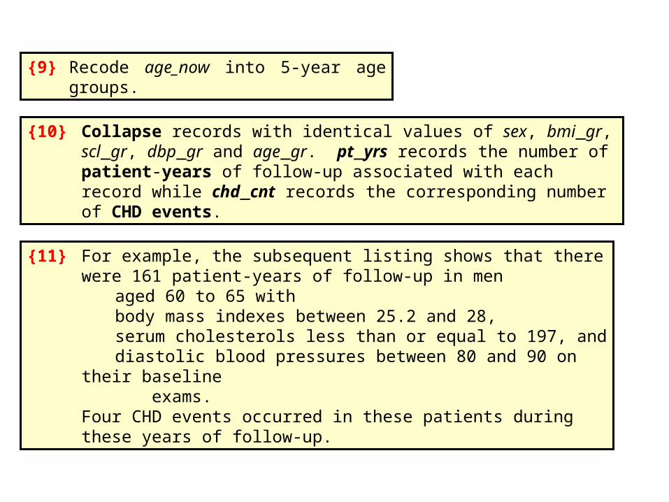
{10} Collapse records with identical values of sex, bmi_gr, scl_gr, dbp_gr and age_gr. pt_yrs records the number of patient-years of follow-up associated with each record while chd_cnt records the corresponding number of CHD events.
{11} For example, the subsequent listing shows that there were 161 patient-years of follow-up in men
aged 60 to 65 withbody mass indexes between 25.2 and 28,serum cholesterols less than or equal to 197, anddiastolic blood pressures between 80 and 90 on their
baseline exams. Four CHD events occurred in these patients during these years of follow-up.
{9} Recode age_now into 5-year age groups.
. * Statistics > Summaries... > Tables > Table of summary statistics (table).
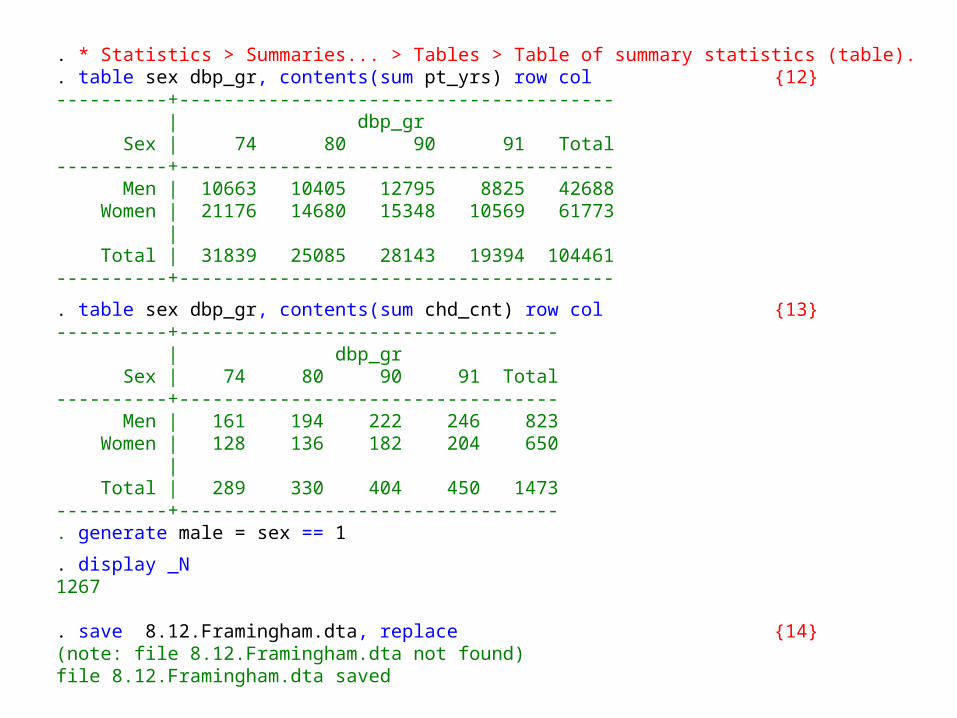
. table sex dbp_gr, contents(sum pt_yrs) row col {12}----------+--------------------------------------- | dbp_gr Sex | 74 80 90 91 Total----------+--------------------------------------- Men | 10663 10405 12795 8825 42688 Women | 21176 14680 15348 10569 61773 | Total | 31839 25085 28143 19394 104461----------+---------------------------------------
. table sex dbp_gr, contents(sum chd_cnt) row col {13}----------+---------------------------------- | dbp_gr Sex | 74 80 90 91 Total----------+---------------------------------- Men | 161 194 222 246 823 Women | 128 136 182 204 650 | Total | 289 330 404 450 1473----------+----------------------------------. generate male = sex == 1
. display _N1267 . save 8.12.Framingham.dta, replace {14}(note: file 8.12.Framingham.dta not found)file 8.12.Framingham.dta saved
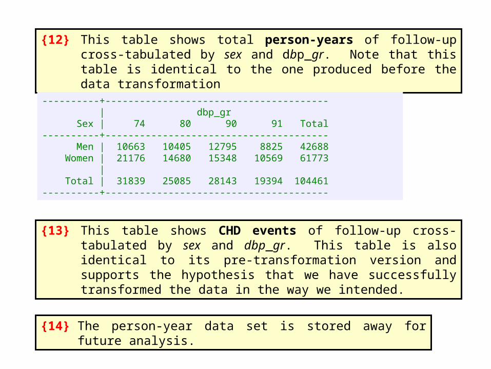
{12} This table shows total person-years of follow-up cross-tabulated by sex and dbp_gr. Note that this table is identical to the one produced before the data transformation
----------+--------------------------------------- | dbp_gr Sex | 74 80 90 91 Total----------+--------------------------------------- Men | 10663 10405 12795 8825 42688 Women | 21176 14680 15348 10569 61773 | Total | 31839 25085 28143 19394 104461----------+---------------------------------------
{13} This table shows CHD events of follow-up cross-tabulated by sex and dbp_gr. This table is also identical to its pre-transformation version and supports the hypothesis that we have successfully transformed the data in the way we intended.
{14} The person-year data set is stored away for future analysis.
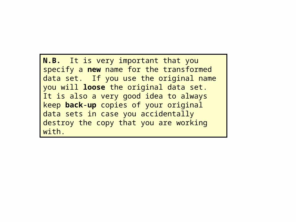
N.B. It is very important that you specify a new name for the transformed data set. If you use the original name you will loose the original data set. It is also a very good idea to always keep back-up copies of your original data sets in case you accidentally destroy the copy that you are working with.
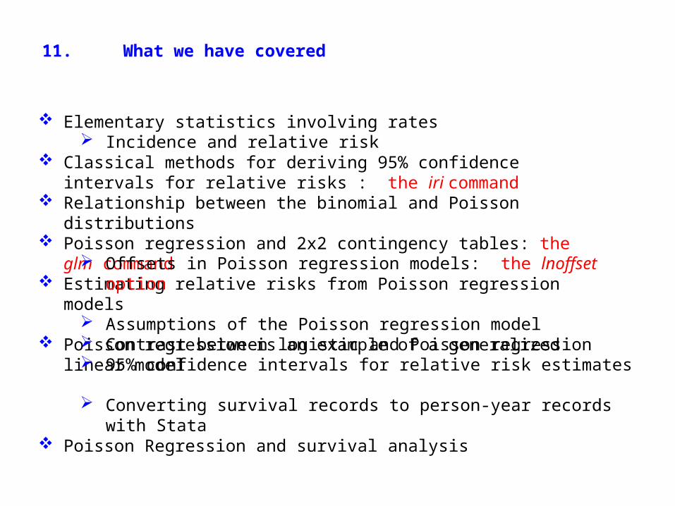
11. What we have covered
Elementary statistics involving rates Classical methods for deriving 95% confidence intervals for
relative risks : the iri command Relationship between the binomial and Poisson distributions Poisson regression and 2x2 contingency tables: the glm
command Estimating relative risks from Poisson regression models
Poisson regression is an example of a generalized linear model
Poisson Regression and survival analysis
Incidence and relative risk
Offsets in Poisson regression models: the lnoffset option
Assumptions of the Poisson regression model Contrast between logistic and Poisson regression 95% confidence intervals for relative risk estimates
Converting survival records to person-year records with Stata

Cited Reference
Levy D, National Heart Lung and Blood Institute., Center for Bio-Medical Communication. 50 Years of Discovery : Medical Milestones from the National Heart, Lung, and Blood Institute's Framingham Heart Study. Hackensack, N.J.: Center for Bio-Medical Communication Inc.; 1999.
For additional references on these notes see.
Dupont WD. Statistical Modeling for Biomedical Researchers: A Simple Introduction to the Analysis of Complex Data. 2nd ed. Cambridge, U.K.: Cambridge University Press; 2009.