count outcomes - poisson regression (chapter 6)wguan/class/pubh7402/notes/lecture6.pdf · count...
TRANSCRIPT
Count outcomes - Poisson regression (Chapter 6)
bull Exponential family
bull Poisson distribution
bull Examples of count data as outcomes of interest
bull Poisson regression
bull Variable follow-up times - Varying number ldquoat riskrdquo - offset
bull Overdispersion - pseudo likelihood
bull Using Poisson regression with robust standard errors in place of binomial
log models
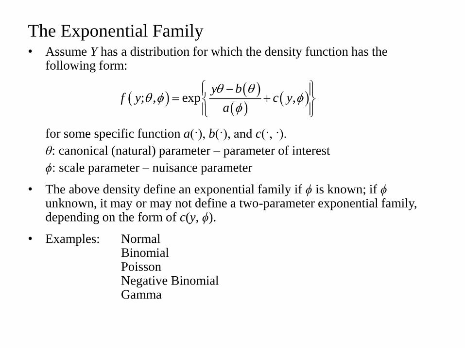
The Exponential Family bull Assume Y has a distribution for which the density function has the
following form
for some specific function a() b() and c( )
θ canonical (natural) parameter ndash parameter of interest
ϕ scale parameter ndash nuisance parameter
bull The above density define an exponential family if ϕ is known if ϕ unknown it may or may not define a two-parameter exponential family depending on the form of c(y ϕ)
bull Examples Normal Binomial Poisson Negative Binomial Gamma
exp
y bf y c y
a
Properties of Exponential Family and Generalized Linear
Models
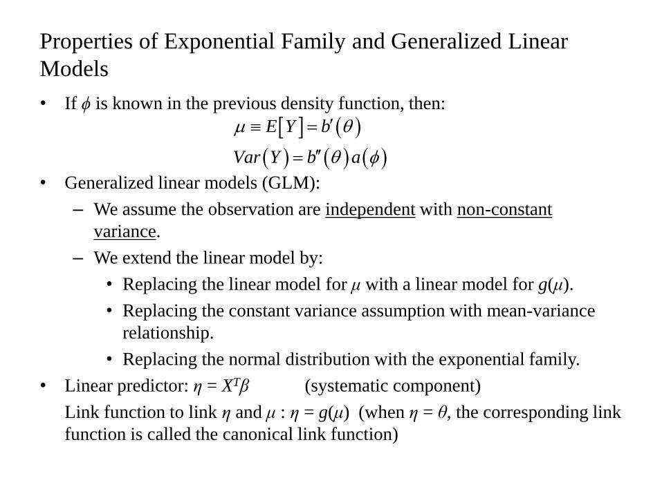
bull If ϕ is known in the previous density function then
bull Generalized linear models (GLM)
ndash We assume the observation are independent with non-constant
variance
ndash We extend the linear model by
bull Replacing the linear model for μ with a linear model for g(μ)
bull Replacing the constant variance assumption with mean-variance
relationship
bull Replacing the normal distribution with the exponential family
bull Linear predictor η = XTβ (systematic component)
Link function to link η and μ η = g(μ) (when η = θ the corresponding link
function is called the canonical link function)
E Y b
Var Y b a
Poisson distribution
bull The Poisson distribution Y sim Poisson(μ) Pr(119884 = 119910) = 119890minus120583120583119910
119910 μ gt 0 is the
most widely-used distribution for counts
bull The Poisson distribution assigns a positive probability to every nonnegative
integer 0 1 2 so that every nonnegative integer becomes a
mathematical possibility (albeit practically zero possibility for most count
values)
bull The Poisson is different than the binomial Bin(n π) which takes on
numbers only up to some n and leads to a proportion (out of n)
bull But the Poisson is similar to the binomial in that it can be show that the
Poisson is the limiting distribution of a Binomial for large n and small π
Furthermore because of the simple form of the Poisson distribution it is
often computationally preferred over the Binomial
Examples of count data
bull Number of visits to emergency room during last year A study looks at the
effectiveness of a new treatment compared to standard care on reducing
emergency room visits controlling for demographics and alcohol and drug
use of individuals (from VGSM)
bull Number of damage reports on ships out to sea in the 1960-80 Look for
systematic variables influencing the likelihood of damage occurring to the
ship (from McCullagh and Nelder 1989)
bull Length of stay (in days) of hospital admissions Look for systematic
variables (ie insurance type type of admission demographics) related to
the average length of stay (from Hardin and Hilbe 2007)
bull Number of homicides within each census tract throughout the Twin Cities
area Look at whether there are relationships between homicide rate and
density of alcohol outlets (Jones-Webb R and Wall MM Neighborhood
RacialEthnic Concentration Social Disadvantage and Homicide Risk An
Ecological Analysis of 10 Cities Journal of Urban Health 2008
Examples of count data
bull Number of injuries that resulted in lost work time during the construction of
the Denver Airport Look at characteristic of construction contracts and see
if there are things that are related to higher injury rates (form Lowery et al
Am Journal of Industrial Medicine 1998)
bull Deaths from coronary heart disease after 10 years in a population of British
male doctors Look at how smoking is related to the risk of death Have
person time at risk (from Breslow and Day 1987)
bull Count of number of abstainers of alcohol and how this is related to
treatment We can use Poisson regression (with robust standard errors) to
estimate common risks in places where we might have computational
problems using binomial regression
The Poisson Regression model
Let Yi be the observed count for experimental unit i
Yi|Xi sim Poi(μi)
log(μi) = Xiβ
The log link is the most commonly used indicating we think that the covariates
influence the mean of the counts (μ) in a multiplicative way ie as a covariate
increases by 1 unit the log of the mean increases by β units and this implies the
mean increases by a ldquofold-changerdquo of or ldquoscale factorrdquo of exp(β)
The log link is the canonical link in GLM for Poisson distribution
Poisson regression for modeling rates
Often we are modeling the count of events within a particular time period or
within a particular region or within a particular risk group of people In each of
these cases what is of interest is to model the RATE
So given for example a specific time period t we want to model the events
occurring in the time period t Thus the Poisson mean μ is better described as μ
= λlowastt where λ is the RATE of events
The term log(ti) is known as the offset and it provides the adjustment for the
variable risk sets (eg varying time periods followed for each person or
variable numbers of people at risk) It can be thought of as a predictor but it
does not have a parameter in front of it to be estimated so it must be treated
different from other predictors in the software
Poisson regression produces relative rates
Let Yi be the count of events within a risk set ti and Xi predictors of interest
Consider
Now a change of one unit in a predictor variable relates to β unit change in
the log RATE (ie log(λi)) so if we exponentiate this we have a Relative rate
(or Rate ratio)
Over and Under dispersion
bull Recall that the if Y ~ Poi(μ) this means that E(Y) = μ AND Var(Y) = μ It is
quite common for the equality of the mean and variance to be incorrect for
count data In other words Poisson distributional assumption is often not
strictly correct
bull A common cause of overdispersion is there are other variable causing
variability in the outcome which are not being included in the model
unexplained random variation Underdispersion does not have an obvious
explanation
bull A common solution is to assume that the variance is proportional to the
mean ie Var(Y) = φμ and estimate the proportionality factor φ which is
called the scale parameter from the data
bull Use the Goodness of fit tests (Pearson or the Residual Deviance) to estimate
the φ 120593 = X2(n minus p) or 120593 = Residual Deviance(n minus p)
Adjusting for overunder-dispersion
bull If 120593 gtgt 1 we say the data exhibits overdispersion and if it is ltlt 1 it is called
underdispersion Note when φ = 1 this means E(Y) = Var(Y ) which is
supportive of the Poisson assumption
bull There is no clear cut decision rules when to decide that there is definitely
overunder dispersion Common rule of thumb is gt 2
bull When controlling for overunder dispersion basically the parameter
estimates do not change but the standard errors do All standard errors are
multiplied by sqrt(120593 ) hence they get wider in the case of overdispersion and
smaller with underdispersion
bull In SAS simply add scale = deviance OR scale = pearson to the model
statement
bull In Stata add scale(x2) or scale(dev) in the glm function
Using Poisson regression for incidence rates
The data show the incidence of nonmelanoma skin cancer among women in
Minneapolis-St Paul Minnesota and Dallas-Fort Worth Texas in 1970 One
would expect sun exposure to be greater in Texas than in Minnesota
--Data from Kleinbaum D Kupper L and Muller K (1989) Applied regression analysis and
other multivariate methods PWS-Kent Boston Massachusetts And adapted from Scotto Kopf
and Ruvbach (1974) input case town str5 age ageyrs pop
1 0 15-24 195 172675
16 0 25-34 295 123065
30 0 35-44 395 96216
71 0 45-54 495 92051
102 0 55-64 595 72159
130 0 65-74 695 54722
133 0 75-84 795 32185
40 0 85+ 895 8328
4 1 15-24 195 181343
38 1 25-34 295 146207
119 1 35-44 395 121374
221 1 45-54 495 111353
259 1 55-64 595 83004
310 1 65-74 695 55932
226 1 75-84 795 29007
65 1 85+ 895 7583
end
town 1 = Dallas 0 = MSP
Skin Cancer data 0
00
20
04
00
60
08
Skin
ca
nce
r ca
sep
op
20 40 60 80 100ageyrs
MSP Dallas
-12
-10
-8-6
-4
log(S
kin
cance
r case
pop
)
20 40 60 80 100ageyrs
-12
-10
-8-6
-4
log(S
kin
cance
r case
pop
)
3 35 4 45logage
Using Poisson regression for incidence rates SAS data skin1 set skin
logpop = log(pop) by default log is natural log in SAS
logage = log(ageyrs)
run
Using Poisson regression
categorical age
proc genmod data = skin1
class ageyrs
model case = ageyrs town dist = poisson link = log offset = logpop
estimate rsquoage adjusted RR of skincancer in Dallas vs MSPrsquo town 1
run
Continuous age
proc genmod data = skin1
model case = ageyrs town dist = poisson link = log offset = logpop
estimate rsquoage adjusted RR of skincancer in Dallas vs MSPrsquo town 1
run
Log transformed continuous age
proc genmod data = skin1
model case = logage town dist = poisson link = log offset = logpop
estimate rsquoage adjusted RR of skincancer in Dallas vs MSPrsquo town 1
run
Using Binomial regression with log link - practically same answer
proc genmod data = skin1
class ageyrs
model casepop = ageyrs town dist = binomial link = log
estimate rsquoage adjusted RR of skincancer in Dallas vs MSPrsquo town 1
run
Treating age as categorical glm case iage_cat town family(poisson) link(log) offset(logpop)
Generalized linear models No of obs = 16
Optimization ML Residual df = 7
Scale parameter = 1
Deviance = 8258494053 (1df) Deviance = 1179785
Pearson = 8127296469 (1df) Pearson = 1161042
Variance function V(u) = u [Poisson]
Link function g(u) = ln(u) [Log]
AIC = 7531475
Log likelihood = -5125179981 BIC = -1114963
------------------------------------------------------------------------------
| OIM
case | Coef Std Err z Pgt|z| [95 Conf Interval]
-------------+----------------------------------------------------------------
age_cat |
2 | 2630202 4674615 563 0000 1713994 354641
3 | 3847367 4546594 846 0000 2956251 4738483
4 | 4595197 4510287 1019 0000 3711197 5479197
5 | 5087289 4503011 1130 0000 4204715 5969863
6 | 5645412 4497475 1255 0000 4763924 6526901
7 | 6058534 4503204 1345 0000 5175923 6941146
8 | 617419 4577405 1349 0000 5277035 7071345
|
town | 8038983 0522048 1540 0000 7015788 9062177
_cons | -1165761 4487091 -2598 0000 -1253706 -1077816
logpop | 1 (offset)
------------------------------------------------------------------------------
Treating age as categorical Risk (Rate) Ratio glm eform
Generalized linear models No of obs = 16
Optimization ML Residual df = 7
Scale parameter = 1
Deviance = 8258494053 (1df) Deviance = 1179785
Pearson = 8127296469 (1df) Pearson = 1161042
Variance function V(u) = u [Poisson]
Link function g(u) = ln(u) [Log]
AIC = 7531475
Log likelihood = -5125179981 BIC = -1114963
------------------------------------------------------------------------------
| OIM
case | IRR Std Err z Pgt|z| [95 Conf Interval]
-------------+----------------------------------------------------------------
age_cat |
2 | 1387657 6486763 563 0000 555109 3468855
3 | 4686951 2130966 846 0000 1922577 1142608
4 | 9900766 446553 1019 0000 4090274 2396543
5 | 1619502 7292636 1130 0000 6700151 391452
6 | 2829902 1272742 1255 0000 1172049 6832777
7 | 4277481 1926237 1345 0000 1769598 1033955
8 | 4801938 2198042 1349 0000 1957885 1177731
|
town | 2234234 1166376 1540 0000 2016935 2474944
_cons | 865e-06 388e-06 -2598 0000 359e-06 0000208
logpop | 1 (offset)
------------------------------------------------------------------------------
Treating age as continuous glm case ageyrs town family(poisson) link(log) offset(logpop)
Generalized linear models No of obs = 16
Optimization ML Residual df = 13
Scale parameter = 1
Deviance = 190561268 (1df) Deviance = 1465856 lt--
Pearson = 1481964085 (1df) Pearson = 1139972
Variance function V(u) = u [Poisson]
Link function g(u) = ln(u) [Log]
AIC = 181754 lt--
Log likelihood = -1424031868 BIC = 1545176
------------------------------------------------------------------------------
| OIM
case | Coef Std Err z Pgt|z| [95 Conf Interval]
-------------+----------------------------------------------------------------
ageyrs | 0600283 0013123 4574 0000 0574562 0626003
town | 8192832 0521801 1570 0000 7170121 9215543
_cons | -1031721 0955464 -10798 0000 -1050448 -1012994
logpop | 1 (offset)
------------------------------------------------------------------------------
lincom town rrr
( 1) [case]town = 0
------------------------------------------------------------------------------
case | RRR Std Err z Pgt|z| [95 Conf Interval]
-------------+----------------------------------------------------------------
(1) | 2268873 11839 1570 0000 2048304 2513194
------------------------------------------------------------------------------
Treating log(age) as continuous glm case logage town family(poisson) link(log) offset(logpop)
Generalized linear models No of obs = 16
Optimization ML Residual df = 13
Scale parameter = 1
Deviance = 4020069588 (1df) Deviance = 3092361 lt--
Pearson = 3436515837 (1df) Pearson = 2643474
Variance function V(u) = u [Poisson]
Link function g(u) = ln(u) [Log]
AIC = 8777863 lt--
Log likelihood = -6722290072 BIC = 4157042
------------------------------------------------------------------------------
| OIM
case | Coef Std Err z Pgt|z| [95 Conf Interval]
-------------+----------------------------------------------------------------
logage | 3313291 0820583 4038 0000 315246 3474122
town | 8095186 0521754 1552 0000 7072567 9117806
_cons | -2010271 3423286 -5872 0000 -2077367 -1943176
logpop | 1 (offset)
------------------------------------------------------------------------------
lincom town rrr
( 1) [case]town = 0
------------------------------------------------------------------------------
case | RRR Std Err z Pgt|z| [95 Conf Interval]
-------------+----------------------------------------------------------------
(1) | 2246826 1172291 1552 0000 2028419 248875
------------------------------------------------------------------------------
Binomial regression binreg case iage_cat town rr n(pop)
Generalized linear models No of obs = 16
Optimization MQL Fisher scoring Residual df = 7
(IRLS EIM) Scale parameter = 1
Deviance = 8281933795 (1df) Deviance = 1183133
Pearson = 8150373408 (1df) Pearson = 1164339
Variance function V(u) = u(1-upop) [Binomial]
Link function g(u) = ln(upop) [Log]
BIC = -1112619
------------------------------------------------------------------------------
| EIM
case | Risk Ratio Std Err z Pgt|z| [95 Conf Interval]
-------------+----------------------------------------------------------------
age_cat |
2 | 1387658 6485948 563 0000 5551734 3468456
3 | 4687123 2130752 846 0000 1922882 114251
4 | 9901094 4465057 1019 0000 4090913 2396327
5 | 16195 7291578 1130 0000 670099 3914018
6 | 2829974 1272581 1255 0000 1172235 6832037
7 | 4276687 192555 1346 0000 1769537 1033607
8 | 480063 2196807 1349 0000 1957859 1177104
|
town | 2233754 1164364 1542 0000 2016814 247403
_cons | 865e-06 388e-06 -2598 0000 359e-06 0000209
------------------------------------------------------------------------------
Similar results as Poisson regression
Comparing models
bull FitzmauriceGM (1997) Model selection with overdispersed data The
Statistician 46(1)81-91 recommends using Adjusted Information criterion
to choose model in cases with overdispersion
bull The general form of information criterion is = -2logL + penalty factor
AIC = -2logL + 2p
SC = Schwarzrsquos Criterion = BIC = - 2logL + 2plog(n)
AICC (Corrected AIC) = -2logL + 2p(nn-p)
bull Recall that if 120583119894 is small (less than 5) then the Deviance and Pearson are not
good measures of the goodness-of-fit and using them as a measure of
overdispersion is not recommended
bull This is the same rule of thumb that tells us not to use the chi-square test when
expected cell sizes in a table are lt 5
Note In Stata the AIC and BIC in -glm- output use different formula from -
estat ic- command The latter is closer to the SAS output (if not the same)
Ship damage example
bull From McCullagh and Nelder (1989) Sec 632
bull Each row represents the AGGREGATED number of months of service and
number of damage incidents to all ships in the fleet particular type built in
the particular year (60-64 65-69 70-74 75-79) and operating during the
particular time period (60-74 75-79)
bull Notice there are some structural zeros (0) under service because it was not
possible for a ship built between 75-79 to operate between 1960-1974
index shiptype year period months damage
1 A 60 60 127 0
2 A 60 75 63 0
3 A 65 60 1095 3
4 A 65 75 1095 4
5 A 70 60 1512 6
6 A 70 75 3353 18
7 A 75 60 0 0
8 A 75 75 2244 11
9 B 60 60 44882 39
10 B 60 75 17176 29
Ship damage example Stata output glm damage itype iyear iperiod family(poisson) link(log) offset(logmonths)
Generalized linear models No of obs = 34
Optimization ML Residual df = 25
Scale parameter = 1
Deviance = 3869504856 (1df) Deviance = 1547802
Pearson = 422752462 (1df) Pearson = 169101
Variance function V(u) = u [Poisson]
Link function g(u) = ln(u) [Log]
AIC = 4545928
Log likelihood = -6828076994 BIC = -4946396
------------------------------------------------------------------------------
| OIM
damage | Coef Std Err z Pgt|z| [95 Conf Interval]
-------------+----------------------------------------------------------------
type |
2 | -5433442 1775899 -306 0002 -8914141 -1952744
3 | -6874015 3290472 -209 0037 -1332322 -0424808
4 | -0759614 2905787 -026 0794 -6454851 4935623
5 | 3255796 2358794 138 0168 -1367355 7878948
|
year |
65 | 6971404 1496414 466 0000 4038486 9904321
70 | 8184267 1697737 482 0000 4856764 1151177
75 | 4534269 2331705 194 0052 -0035789 9104327
|
75period | 3844667 1182722 325 0001 1526575 6162759
_cons | -6405901 2174441 -2946 0000 -6832084 -5979719
logmonths | 1 (offset)
------------------------------------------------------------------------------
Ship damage example Stata output relative rate for B vs C type
lincom 2type-3type eform
( 1) [damage]2type - [damage]3type = 0
------------------------------------------------------------------------------
damage | exp(b) Std Err z Pgt|z| [95 Conf Interval]
-------------+----------------------------------------------------------------
(1) | 115495 3449144 048 0630 6432213 2073796
------------------------------------------------------------------------------
relative rate for 1975- vs 1960-64
lincom 75year eform
( 1) [damage]75year = 0
------------------------------------------------------------------------------
damage | exp(b) Std Err z Pgt|z| [95 Conf Interval]
-------------+----------------------------------------------------------------
(1) | 1573696 3669394 194 0052 9964275 2485398
------------------------------------------------------------------------------
Note The Pearson X2 was 169 and Deviance 155 indicating moderate
overdispersion In SAS this can be addressed in Proc Genmod by using the
scale option in the model statement scale = p uses the Pearson while scale = d
uses the deviance to adjust the standard error estimates In Stata use scale(x2)
or scale(dev) option
Ship damage example correct for overdispersion
glm damage itype iyear iperiod family(poisson) link(log) offset(logmonths) scale(x2)
------------------------------------------------------------------------------
| OIM
damage | Coef Std Err z Pgt|z| [95 Conf Interval]
-------------+----------------------------------------------------------------
type |
2 | -5433442 2309359 -235 0019 -9959702 -0907183
3 | -6874015 4278892 -161 0108 -1526049 1512459
4 | -0759614 3778651 -020 0841 -8165634 6646406
5 | 3255796 3067348 106 0288 -2756096 9267688
|
year |
65 | 6971404 1945919 358 0000 3157472 1078534
70 | 8184267 2207717 371 0000 3857221 1251131
75 | 4534269 3032122 150 0135 -1408581 1047712
|
75period | 3844667 1537997 250 0012 0830247 6859086
_cons | -6405901 2827618 -2265 0000 -6960104 -5851699
logmonths | 1 (offset)
------------------------------------------------------------------------------
(Standard errors scaled using square root of Pearson X2-based dispersion)
Ship damage example Stata output relative rate for B vs C type
lincom 2type-3type eform
( 1) [damage]2type - [damage]3type = 0
------------------------------------------------------------------------------
damage | exp(b) Std Err z Pgt|z| [95 Conf Interval]
-------------+----------------------------------------------------------------
(1) | 115495 4485226 037 0711 5395116 247244
------------------------------------------------------------------------------
relative rate for 1975- vs 1960-64
lincom 75year eform
( 1) [damage]75year = 0
------------------------------------------------------------------------------
damage | exp(b) Std Err z Pgt|z| [95 Conf Interval]
-------------+----------------------------------------------------------------
(1) | 1573696 4771638 150 0135 8686126 285112
------------------------------------------------------------------------------
Note the coefficient estimates are the same as previous output but the standard
errors and test p-values are now more conservative
Poisson regression with common risks
Previously we saw that OR and RR were quite different when the prevalence of
the risk was not small bigger than 10 In order to estimate an adjusted RR we
could use the Binomial model with a log link But sometimes there are
computational difficulties with this model An alternative is to use the Poisson
model AND to utilize the ROBUST STANDARD ERRORS Regular standard
errors for Poisson are known to be too conservative in these cases of
approximating binomial data with common risk
Binomial Regression
proc genmod data = birthwgt2 descending
class c_baseline_bmi (ref = 2) param = ref
model hibwt = totalweightgain c_baseline_bmidist=binomial link=log type3
run
Poisson Regression
proc genmod data = birthwgt2 descending
class c_baseline_bmi (ref = 2) id param = ref lt- need to generate an lsquoidrsquo variable for every sample
model hibwt = totalweightgain c_baseline_bmidist=poisson link=log type3
repeated sub = id type=ind lt- This is the statement to obtain robust std errors
run
Birthweight example log link glm hibwt totalweightgain ib2c_baseline_bmi fam(bin) link(log) eform iter(100)
Iteration 100 log likelihood = -10390036 (not concave)
convergence not achieved
AIC = 1042004
Log likelihood = -1039003635 BIC = -1310099
---------------------------------------------------------------------------------
| OIM
hibwt | Risk Ratio Std Err z Pgt|z| [95 Conf Interval]
----------------+----------------------------------------------------------------
totalweightgain | 1024364 878e-10 28e+07 0000 1024364 1024364
|
c_baseline_bmi |
1 | 0617007 0352668 -487 0000 0201262 1891555
3 | 6152626 0750599 -398 0000 4844141 7814554
4 | 1855169
|
_cons | 1368256 765e-09 -36e+07 0000 1368255 1368256
---------------------------------------------------------------------------------
Warning parameter estimates produce inadmissible mean estimates in one or
more observations
Warning convergence not achieved
Birthweight example Poisson regression with regular SE glm hibwt totalweightgain ib2c_baseline_bmi fam(poisson) link(log) eform
Generalized linear models No of obs = 2000
Optimization ML Residual df = 1995
Scale parameter = 1
Deviance = 963011489 (1df) Deviance = 4827125
Pearson = 1643646513 (1df) Pearson = 823883
Variance function V(u) = u [Poisson]
Link function g(u) = ln(u) [Log]
AIC = 7465057
Log likelihood = -7415057445 BIC = -1420079
---------------------------------------------------------------------------------
| OIM
hibwt | IRR Std Err z Pgt|z| [95 Conf Interval]
----------------+----------------------------------------------------------------
totalweightgain | 1032877 0046171 724 0000 1023868 1041966
|
c_baseline_bmi |
1 | 187722 1100813 -285 0004 0594793 5924677
3 | 1875006 3199926 368 0000 1341945 2619814
4 | 2387442 3428306 606 0000 1801783 3163466
|
_cons | 0334007 0064157 -1770 0000 022922 0486695
---------------------------------------------------------------------------------
Birthweight example Poisson regression with robust SE glm hibwt totalweightgain ib2c_baseline_bmi fam(poisson) link(log) eform robust
Generalized linear models No of obs = 2000
Optimization ML Residual df = 1995
Scale parameter = 1
Deviance = 963011489 (1df) Deviance = 4827125
Pearson = 1643646513 (1df) Pearson = 823883
Variance function V(u) = u [Poisson]
Link function g(u) = ln(u) [Log]
AIC = 7465057
Log pseudolikelihood = -7415057445 BIC = -1420079
---------------------------------------------------------------------------------
| Robust
hibwt | IRR Std Err z Pgt|z| [95 Conf Interval]
----------------+----------------------------------------------------------------
totalweightgain | 1032877 0038243 874 0000 1025409 10404
|
c_baseline_bmi |
1 | 187722 1077046 -292 0004 0609737 5779468
3 | 1875006 2884014 409 0000 1386999 2534714
4 | 2387442 3093241 672 0000 1852032 3077634
|
_cons | 0334007 005491 -2068 0000 0242002 0460989
---------------------------------------------------------------------------------
Other count models
bull Zero-truncated Poisson
Example A study by the county traffic court on the number of tickets
received by teenagers as predicted by school performance amount of driver
training and gender Only individuals who have received at least one
citation are in the traffic court files
SAS proc nlmixed
(httpwwwatsuclaedustatsasfaqzt_nlmixedhtm)
Stata tpoisson y x1 x2 inflate(x1)
(httpwwwatsuclaedustatsasfaqzt_nlmixedhtm)
Other count models
bull Zero-inflated Poisson
Example The state wildlife biologists want to model how many fish are
being caught by fishermen at a state park Visitors are asked whether or not
they have a camper how many people were in the group were there
children in the group and how many fish were caught Some visitors do not
fish but there is no data on whether a person fished or not Some visitors
who did fish did not catch any fish so there are excess zeros in the data
because of the people that did not fish
SAS proc genmod data = hellip model y = x1 x2 dist=zip zeromodel x1 link = logit
(httpwwwatsuclaedustatsasdaezipreghtm)
Stata zip y x1 x2 inflate(x1)
(httpwwwatsuclaedustatstatadaeziphtm)
Other count models
bull Negative binomial model
ndash Have one more parameter than the Poisson the second parameter can be
used to adjust the variance independently of the mean
ndash Alternative solution to overdispersed Poisson
SAS proc genmod data = hellip model y = x1 x2 dist=negbin
Stata glm y x1 x2 family(nb)
bull Zero-inflated negative binomial model
bull Zero-truncated negative binomial model
( Check the UCLA website for examples)
Estimation and Goodness of fit for GLM
bull Estimation
ndash MLE maximize the log-likelihood
ndash Iterated Weighted Least Squares (IWLS) analogous to weighted least
squares with the weights updated iteratively
GLM fits using IWLS is more general than MLE (see eg quasi-likelihood
if you want to know more details)
bull Goodness of fit
ndash Pearsonrsquos X2 (does not depend on distribution assumption)
where mi = 1 for Normal and Poisson ni for Binomial
ndash Deviance (does not depend on ϕ but depends on log-likelihood)
where (natural parameter for the saturated model)
2
2
1
ˆ
ˆ
ni i
i i i
YX
V m
1
ˆ ˆ 2
ˆ ˆ2n
i i i i i i
i
D Y l Y Y l Y
m Y b b
i ib Y
Residuals bull Types of Residuals
ndash Pearson residual
ndash Deviance residual
ndash Response residual
ndash Working residual
ndash Partial residual
Note residual diagnostics non-informative for binary data
bull Overdispersion Var(Y) gt a(ϕ)V(μ) for any GLM
check if X2(n-p) or D(n-p) gtgt 1
ˆ
ˆ
P i ii
i
Yr
V
ˆD
i i i ir sign Y d
ˆ
ˆˆ
W ii i i
i
r Y
ˆR
i i ir Y
ˆ ˆˆˆ
T iki i i ik k
i
r Y x
Checking outliers
Check for observations with large (standardized) Pearson or deviance
residuals
Deviance residual is generally preferred to the Pearson residual since its
distributional properties are closer to the residuals in linear regression
-2-1
01
2
sta
nda
rdiz
ed
de
via
nce
re
sid
ua
l
0 100 200 300predicted mean case
-2-1
01
2
sta
nda
rdiz
ed
Pe
ars
on
re
sid
ua
l
0 100 200 300predicted mean case
Checking the variance function
The x-axis is ldquoconstant-information scalerdquo for Poisson errors See McCullagh
and Nelder ldquoGeneralized Linear Modelsrdquo (Chapter 1261)
Positive trend indicates the current variance function increases too slowly with
the mean
05
11
52
abso
lute
sta
nda
rdiz
ed d
evia
nce
resid
ual
0 10 20 30 402sqrt(mu)
Checking for linearity lowess plot
Other approach to check departure from linearity
ndash Add polynomial terms (eg age^2) and test for their statistical
significance
ndash Group continuous predictor into categories (eg age_cat)
-26
-24
-22
-2-1
8-1
6
low
ess h
ibw
t ag
e_lm
p
15 20 25 30 35 40age_lmp
Other Diagnostics
bull Checking the link function the simplest method is to include as
covariate and assessing the fall in deviance (Hinkley 1985)
bull Partial residual is helpful to assess the form of covariates ie plot partial
residual against the corresponding predictor
bull Checking influential points modified Cookrsquos distance (gt 4(n-p) to be
problematic)
2
02
46
81
Coo
ks
dis
tan
ce
0 5 10 15observation
The Exponential Family bull Assume Y has a distribution for which the density function has the
following form
for some specific function a() b() and c( )
θ canonical (natural) parameter ndash parameter of interest
ϕ scale parameter ndash nuisance parameter
bull The above density define an exponential family if ϕ is known if ϕ unknown it may or may not define a two-parameter exponential family depending on the form of c(y ϕ)
bull Examples Normal Binomial Poisson Negative Binomial Gamma
exp
y bf y c y
a
Properties of Exponential Family and Generalized Linear
Models
bull If ϕ is known in the previous density function then
bull Generalized linear models (GLM)
ndash We assume the observation are independent with non-constant
variance
ndash We extend the linear model by
bull Replacing the linear model for μ with a linear model for g(μ)
bull Replacing the constant variance assumption with mean-variance
relationship
bull Replacing the normal distribution with the exponential family
bull Linear predictor η = XTβ (systematic component)
Link function to link η and μ η = g(μ) (when η = θ the corresponding link
function is called the canonical link function)
E Y b
Var Y b a
Poisson distribution
bull The Poisson distribution Y sim Poisson(μ) Pr(119884 = 119910) = 119890minus120583120583119910
119910 μ gt 0 is the
most widely-used distribution for counts
bull The Poisson distribution assigns a positive probability to every nonnegative
integer 0 1 2 so that every nonnegative integer becomes a
mathematical possibility (albeit practically zero possibility for most count
values)
bull The Poisson is different than the binomial Bin(n π) which takes on
numbers only up to some n and leads to a proportion (out of n)
bull But the Poisson is similar to the binomial in that it can be show that the
Poisson is the limiting distribution of a Binomial for large n and small π
Furthermore because of the simple form of the Poisson distribution it is
often computationally preferred over the Binomial
Examples of count data
bull Number of visits to emergency room during last year A study looks at the
effectiveness of a new treatment compared to standard care on reducing
emergency room visits controlling for demographics and alcohol and drug
use of individuals (from VGSM)
bull Number of damage reports on ships out to sea in the 1960-80 Look for
systematic variables influencing the likelihood of damage occurring to the
ship (from McCullagh and Nelder 1989)
bull Length of stay (in days) of hospital admissions Look for systematic
variables (ie insurance type type of admission demographics) related to
the average length of stay (from Hardin and Hilbe 2007)
bull Number of homicides within each census tract throughout the Twin Cities
area Look at whether there are relationships between homicide rate and
density of alcohol outlets (Jones-Webb R and Wall MM Neighborhood
RacialEthnic Concentration Social Disadvantage and Homicide Risk An
Ecological Analysis of 10 Cities Journal of Urban Health 2008
Examples of count data
bull Number of injuries that resulted in lost work time during the construction of
the Denver Airport Look at characteristic of construction contracts and see
if there are things that are related to higher injury rates (form Lowery et al
Am Journal of Industrial Medicine 1998)
bull Deaths from coronary heart disease after 10 years in a population of British
male doctors Look at how smoking is related to the risk of death Have
person time at risk (from Breslow and Day 1987)
bull Count of number of abstainers of alcohol and how this is related to
treatment We can use Poisson regression (with robust standard errors) to
estimate common risks in places where we might have computational
problems using binomial regression
The Poisson Regression model
Let Yi be the observed count for experimental unit i
Yi|Xi sim Poi(μi)
log(μi) = Xiβ
The log link is the most commonly used indicating we think that the covariates
influence the mean of the counts (μ) in a multiplicative way ie as a covariate
increases by 1 unit the log of the mean increases by β units and this implies the
mean increases by a ldquofold-changerdquo of or ldquoscale factorrdquo of exp(β)
The log link is the canonical link in GLM for Poisson distribution
Poisson regression for modeling rates
Often we are modeling the count of events within a particular time period or
within a particular region or within a particular risk group of people In each of
these cases what is of interest is to model the RATE
So given for example a specific time period t we want to model the events
occurring in the time period t Thus the Poisson mean μ is better described as μ
= λlowastt where λ is the RATE of events
The term log(ti) is known as the offset and it provides the adjustment for the
variable risk sets (eg varying time periods followed for each person or
variable numbers of people at risk) It can be thought of as a predictor but it
does not have a parameter in front of it to be estimated so it must be treated
different from other predictors in the software
Poisson regression produces relative rates
Let Yi be the count of events within a risk set ti and Xi predictors of interest
Consider
Now a change of one unit in a predictor variable relates to β unit change in
the log RATE (ie log(λi)) so if we exponentiate this we have a Relative rate
(or Rate ratio)
Over and Under dispersion
bull Recall that the if Y ~ Poi(μ) this means that E(Y) = μ AND Var(Y) = μ It is
quite common for the equality of the mean and variance to be incorrect for
count data In other words Poisson distributional assumption is often not
strictly correct
bull A common cause of overdispersion is there are other variable causing
variability in the outcome which are not being included in the model
unexplained random variation Underdispersion does not have an obvious
explanation
bull A common solution is to assume that the variance is proportional to the
mean ie Var(Y) = φμ and estimate the proportionality factor φ which is
called the scale parameter from the data
bull Use the Goodness of fit tests (Pearson or the Residual Deviance) to estimate
the φ 120593 = X2(n minus p) or 120593 = Residual Deviance(n minus p)
Adjusting for overunder-dispersion
bull If 120593 gtgt 1 we say the data exhibits overdispersion and if it is ltlt 1 it is called
underdispersion Note when φ = 1 this means E(Y) = Var(Y ) which is
supportive of the Poisson assumption
bull There is no clear cut decision rules when to decide that there is definitely
overunder dispersion Common rule of thumb is gt 2
bull When controlling for overunder dispersion basically the parameter
estimates do not change but the standard errors do All standard errors are
multiplied by sqrt(120593 ) hence they get wider in the case of overdispersion and
smaller with underdispersion
bull In SAS simply add scale = deviance OR scale = pearson to the model
statement
bull In Stata add scale(x2) or scale(dev) in the glm function
Using Poisson regression for incidence rates
The data show the incidence of nonmelanoma skin cancer among women in
Minneapolis-St Paul Minnesota and Dallas-Fort Worth Texas in 1970 One
would expect sun exposure to be greater in Texas than in Minnesota
--Data from Kleinbaum D Kupper L and Muller K (1989) Applied regression analysis and
other multivariate methods PWS-Kent Boston Massachusetts And adapted from Scotto Kopf
and Ruvbach (1974) input case town str5 age ageyrs pop
1 0 15-24 195 172675
16 0 25-34 295 123065
30 0 35-44 395 96216
71 0 45-54 495 92051
102 0 55-64 595 72159
130 0 65-74 695 54722
133 0 75-84 795 32185
40 0 85+ 895 8328
4 1 15-24 195 181343
38 1 25-34 295 146207
119 1 35-44 395 121374
221 1 45-54 495 111353
259 1 55-64 595 83004
310 1 65-74 695 55932
226 1 75-84 795 29007
65 1 85+ 895 7583
end
town 1 = Dallas 0 = MSP
Skin Cancer data 0
00
20
04
00
60
08
Skin
ca
nce
r ca
sep
op
20 40 60 80 100ageyrs
MSP Dallas
-12
-10
-8-6
-4
log(S
kin
cance
r case
pop
)
20 40 60 80 100ageyrs
-12
-10
-8-6
-4
log(S
kin
cance
r case
pop
)
3 35 4 45logage
Using Poisson regression for incidence rates SAS data skin1 set skin
logpop = log(pop) by default log is natural log in SAS
logage = log(ageyrs)
run
Using Poisson regression
categorical age
proc genmod data = skin1
class ageyrs
model case = ageyrs town dist = poisson link = log offset = logpop
estimate rsquoage adjusted RR of skincancer in Dallas vs MSPrsquo town 1
run
Continuous age
proc genmod data = skin1
model case = ageyrs town dist = poisson link = log offset = logpop
estimate rsquoage adjusted RR of skincancer in Dallas vs MSPrsquo town 1
run
Log transformed continuous age
proc genmod data = skin1
model case = logage town dist = poisson link = log offset = logpop
estimate rsquoage adjusted RR of skincancer in Dallas vs MSPrsquo town 1
run
Using Binomial regression with log link - practically same answer
proc genmod data = skin1
class ageyrs
model casepop = ageyrs town dist = binomial link = log
estimate rsquoage adjusted RR of skincancer in Dallas vs MSPrsquo town 1
run
Treating age as categorical glm case iage_cat town family(poisson) link(log) offset(logpop)
Generalized linear models No of obs = 16
Optimization ML Residual df = 7
Scale parameter = 1
Deviance = 8258494053 (1df) Deviance = 1179785
Pearson = 8127296469 (1df) Pearson = 1161042
Variance function V(u) = u [Poisson]
Link function g(u) = ln(u) [Log]
AIC = 7531475
Log likelihood = -5125179981 BIC = -1114963
------------------------------------------------------------------------------
| OIM
case | Coef Std Err z Pgt|z| [95 Conf Interval]
-------------+----------------------------------------------------------------
age_cat |
2 | 2630202 4674615 563 0000 1713994 354641
3 | 3847367 4546594 846 0000 2956251 4738483
4 | 4595197 4510287 1019 0000 3711197 5479197
5 | 5087289 4503011 1130 0000 4204715 5969863
6 | 5645412 4497475 1255 0000 4763924 6526901
7 | 6058534 4503204 1345 0000 5175923 6941146
8 | 617419 4577405 1349 0000 5277035 7071345
|
town | 8038983 0522048 1540 0000 7015788 9062177
_cons | -1165761 4487091 -2598 0000 -1253706 -1077816
logpop | 1 (offset)
------------------------------------------------------------------------------
Treating age as categorical Risk (Rate) Ratio glm eform
Generalized linear models No of obs = 16
Optimization ML Residual df = 7
Scale parameter = 1
Deviance = 8258494053 (1df) Deviance = 1179785
Pearson = 8127296469 (1df) Pearson = 1161042
Variance function V(u) = u [Poisson]
Link function g(u) = ln(u) [Log]
AIC = 7531475
Log likelihood = -5125179981 BIC = -1114963
------------------------------------------------------------------------------
| OIM
case | IRR Std Err z Pgt|z| [95 Conf Interval]
-------------+----------------------------------------------------------------
age_cat |
2 | 1387657 6486763 563 0000 555109 3468855
3 | 4686951 2130966 846 0000 1922577 1142608
4 | 9900766 446553 1019 0000 4090274 2396543
5 | 1619502 7292636 1130 0000 6700151 391452
6 | 2829902 1272742 1255 0000 1172049 6832777
7 | 4277481 1926237 1345 0000 1769598 1033955
8 | 4801938 2198042 1349 0000 1957885 1177731
|
town | 2234234 1166376 1540 0000 2016935 2474944
_cons | 865e-06 388e-06 -2598 0000 359e-06 0000208
logpop | 1 (offset)
------------------------------------------------------------------------------
Treating age as continuous glm case ageyrs town family(poisson) link(log) offset(logpop)
Generalized linear models No of obs = 16
Optimization ML Residual df = 13
Scale parameter = 1
Deviance = 190561268 (1df) Deviance = 1465856 lt--
Pearson = 1481964085 (1df) Pearson = 1139972
Variance function V(u) = u [Poisson]
Link function g(u) = ln(u) [Log]
AIC = 181754 lt--
Log likelihood = -1424031868 BIC = 1545176
------------------------------------------------------------------------------
| OIM
case | Coef Std Err z Pgt|z| [95 Conf Interval]
-------------+----------------------------------------------------------------
ageyrs | 0600283 0013123 4574 0000 0574562 0626003
town | 8192832 0521801 1570 0000 7170121 9215543
_cons | -1031721 0955464 -10798 0000 -1050448 -1012994
logpop | 1 (offset)
------------------------------------------------------------------------------
lincom town rrr
( 1) [case]town = 0
------------------------------------------------------------------------------
case | RRR Std Err z Pgt|z| [95 Conf Interval]
-------------+----------------------------------------------------------------
(1) | 2268873 11839 1570 0000 2048304 2513194
------------------------------------------------------------------------------
Treating log(age) as continuous glm case logage town family(poisson) link(log) offset(logpop)
Generalized linear models No of obs = 16
Optimization ML Residual df = 13
Scale parameter = 1
Deviance = 4020069588 (1df) Deviance = 3092361 lt--
Pearson = 3436515837 (1df) Pearson = 2643474
Variance function V(u) = u [Poisson]
Link function g(u) = ln(u) [Log]
AIC = 8777863 lt--
Log likelihood = -6722290072 BIC = 4157042
------------------------------------------------------------------------------
| OIM
case | Coef Std Err z Pgt|z| [95 Conf Interval]
-------------+----------------------------------------------------------------
logage | 3313291 0820583 4038 0000 315246 3474122
town | 8095186 0521754 1552 0000 7072567 9117806
_cons | -2010271 3423286 -5872 0000 -2077367 -1943176
logpop | 1 (offset)
------------------------------------------------------------------------------
lincom town rrr
( 1) [case]town = 0
------------------------------------------------------------------------------
case | RRR Std Err z Pgt|z| [95 Conf Interval]
-------------+----------------------------------------------------------------
(1) | 2246826 1172291 1552 0000 2028419 248875
------------------------------------------------------------------------------
Binomial regression binreg case iage_cat town rr n(pop)
Generalized linear models No of obs = 16
Optimization MQL Fisher scoring Residual df = 7
(IRLS EIM) Scale parameter = 1
Deviance = 8281933795 (1df) Deviance = 1183133
Pearson = 8150373408 (1df) Pearson = 1164339
Variance function V(u) = u(1-upop) [Binomial]
Link function g(u) = ln(upop) [Log]
BIC = -1112619
------------------------------------------------------------------------------
| EIM
case | Risk Ratio Std Err z Pgt|z| [95 Conf Interval]
-------------+----------------------------------------------------------------
age_cat |
2 | 1387658 6485948 563 0000 5551734 3468456
3 | 4687123 2130752 846 0000 1922882 114251
4 | 9901094 4465057 1019 0000 4090913 2396327
5 | 16195 7291578 1130 0000 670099 3914018
6 | 2829974 1272581 1255 0000 1172235 6832037
7 | 4276687 192555 1346 0000 1769537 1033607
8 | 480063 2196807 1349 0000 1957859 1177104
|
town | 2233754 1164364 1542 0000 2016814 247403
_cons | 865e-06 388e-06 -2598 0000 359e-06 0000209
------------------------------------------------------------------------------
Similar results as Poisson regression
Comparing models
bull FitzmauriceGM (1997) Model selection with overdispersed data The
Statistician 46(1)81-91 recommends using Adjusted Information criterion
to choose model in cases with overdispersion
bull The general form of information criterion is = -2logL + penalty factor
AIC = -2logL + 2p
SC = Schwarzrsquos Criterion = BIC = - 2logL + 2plog(n)
AICC (Corrected AIC) = -2logL + 2p(nn-p)
bull Recall that if 120583119894 is small (less than 5) then the Deviance and Pearson are not
good measures of the goodness-of-fit and using them as a measure of
overdispersion is not recommended
bull This is the same rule of thumb that tells us not to use the chi-square test when
expected cell sizes in a table are lt 5
Note In Stata the AIC and BIC in -glm- output use different formula from -
estat ic- command The latter is closer to the SAS output (if not the same)
Ship damage example
bull From McCullagh and Nelder (1989) Sec 632
bull Each row represents the AGGREGATED number of months of service and
number of damage incidents to all ships in the fleet particular type built in
the particular year (60-64 65-69 70-74 75-79) and operating during the
particular time period (60-74 75-79)
bull Notice there are some structural zeros (0) under service because it was not
possible for a ship built between 75-79 to operate between 1960-1974
index shiptype year period months damage
1 A 60 60 127 0
2 A 60 75 63 0
3 A 65 60 1095 3
4 A 65 75 1095 4
5 A 70 60 1512 6
6 A 70 75 3353 18
7 A 75 60 0 0
8 A 75 75 2244 11
9 B 60 60 44882 39
10 B 60 75 17176 29
Ship damage example Stata output glm damage itype iyear iperiod family(poisson) link(log) offset(logmonths)
Generalized linear models No of obs = 34
Optimization ML Residual df = 25
Scale parameter = 1
Deviance = 3869504856 (1df) Deviance = 1547802
Pearson = 422752462 (1df) Pearson = 169101
Variance function V(u) = u [Poisson]
Link function g(u) = ln(u) [Log]
AIC = 4545928
Log likelihood = -6828076994 BIC = -4946396
------------------------------------------------------------------------------
| OIM
damage | Coef Std Err z Pgt|z| [95 Conf Interval]
-------------+----------------------------------------------------------------
type |
2 | -5433442 1775899 -306 0002 -8914141 -1952744
3 | -6874015 3290472 -209 0037 -1332322 -0424808
4 | -0759614 2905787 -026 0794 -6454851 4935623
5 | 3255796 2358794 138 0168 -1367355 7878948
|
year |
65 | 6971404 1496414 466 0000 4038486 9904321
70 | 8184267 1697737 482 0000 4856764 1151177
75 | 4534269 2331705 194 0052 -0035789 9104327
|
75period | 3844667 1182722 325 0001 1526575 6162759
_cons | -6405901 2174441 -2946 0000 -6832084 -5979719
logmonths | 1 (offset)
------------------------------------------------------------------------------
Ship damage example Stata output relative rate for B vs C type
lincom 2type-3type eform
( 1) [damage]2type - [damage]3type = 0
------------------------------------------------------------------------------
damage | exp(b) Std Err z Pgt|z| [95 Conf Interval]
-------------+----------------------------------------------------------------
(1) | 115495 3449144 048 0630 6432213 2073796
------------------------------------------------------------------------------
relative rate for 1975- vs 1960-64
lincom 75year eform
( 1) [damage]75year = 0
------------------------------------------------------------------------------
damage | exp(b) Std Err z Pgt|z| [95 Conf Interval]
-------------+----------------------------------------------------------------
(1) | 1573696 3669394 194 0052 9964275 2485398
------------------------------------------------------------------------------
Note The Pearson X2 was 169 and Deviance 155 indicating moderate
overdispersion In SAS this can be addressed in Proc Genmod by using the
scale option in the model statement scale = p uses the Pearson while scale = d
uses the deviance to adjust the standard error estimates In Stata use scale(x2)
or scale(dev) option
Ship damage example correct for overdispersion
glm damage itype iyear iperiod family(poisson) link(log) offset(logmonths) scale(x2)
------------------------------------------------------------------------------
| OIM
damage | Coef Std Err z Pgt|z| [95 Conf Interval]
-------------+----------------------------------------------------------------
type |
2 | -5433442 2309359 -235 0019 -9959702 -0907183
3 | -6874015 4278892 -161 0108 -1526049 1512459
4 | -0759614 3778651 -020 0841 -8165634 6646406
5 | 3255796 3067348 106 0288 -2756096 9267688
|
year |
65 | 6971404 1945919 358 0000 3157472 1078534
70 | 8184267 2207717 371 0000 3857221 1251131
75 | 4534269 3032122 150 0135 -1408581 1047712
|
75period | 3844667 1537997 250 0012 0830247 6859086
_cons | -6405901 2827618 -2265 0000 -6960104 -5851699
logmonths | 1 (offset)
------------------------------------------------------------------------------
(Standard errors scaled using square root of Pearson X2-based dispersion)
Ship damage example Stata output relative rate for B vs C type
lincom 2type-3type eform
( 1) [damage]2type - [damage]3type = 0
------------------------------------------------------------------------------
damage | exp(b) Std Err z Pgt|z| [95 Conf Interval]
-------------+----------------------------------------------------------------
(1) | 115495 4485226 037 0711 5395116 247244
------------------------------------------------------------------------------
relative rate for 1975- vs 1960-64
lincom 75year eform
( 1) [damage]75year = 0
------------------------------------------------------------------------------
damage | exp(b) Std Err z Pgt|z| [95 Conf Interval]
-------------+----------------------------------------------------------------
(1) | 1573696 4771638 150 0135 8686126 285112
------------------------------------------------------------------------------
Note the coefficient estimates are the same as previous output but the standard
errors and test p-values are now more conservative
Poisson regression with common risks
Previously we saw that OR and RR were quite different when the prevalence of
the risk was not small bigger than 10 In order to estimate an adjusted RR we
could use the Binomial model with a log link But sometimes there are
computational difficulties with this model An alternative is to use the Poisson
model AND to utilize the ROBUST STANDARD ERRORS Regular standard
errors for Poisson are known to be too conservative in these cases of
approximating binomial data with common risk
Binomial Regression
proc genmod data = birthwgt2 descending
class c_baseline_bmi (ref = 2) param = ref
model hibwt = totalweightgain c_baseline_bmidist=binomial link=log type3
run
Poisson Regression
proc genmod data = birthwgt2 descending
class c_baseline_bmi (ref = 2) id param = ref lt- need to generate an lsquoidrsquo variable for every sample
model hibwt = totalweightgain c_baseline_bmidist=poisson link=log type3
repeated sub = id type=ind lt- This is the statement to obtain robust std errors
run
Birthweight example log link glm hibwt totalweightgain ib2c_baseline_bmi fam(bin) link(log) eform iter(100)
Iteration 100 log likelihood = -10390036 (not concave)
convergence not achieved
AIC = 1042004
Log likelihood = -1039003635 BIC = -1310099
---------------------------------------------------------------------------------
| OIM
hibwt | Risk Ratio Std Err z Pgt|z| [95 Conf Interval]
----------------+----------------------------------------------------------------
totalweightgain | 1024364 878e-10 28e+07 0000 1024364 1024364
|
c_baseline_bmi |
1 | 0617007 0352668 -487 0000 0201262 1891555
3 | 6152626 0750599 -398 0000 4844141 7814554
4 | 1855169
|
_cons | 1368256 765e-09 -36e+07 0000 1368255 1368256
---------------------------------------------------------------------------------
Warning parameter estimates produce inadmissible mean estimates in one or
more observations
Warning convergence not achieved
Birthweight example Poisson regression with regular SE glm hibwt totalweightgain ib2c_baseline_bmi fam(poisson) link(log) eform
Generalized linear models No of obs = 2000
Optimization ML Residual df = 1995
Scale parameter = 1
Deviance = 963011489 (1df) Deviance = 4827125
Pearson = 1643646513 (1df) Pearson = 823883
Variance function V(u) = u [Poisson]
Link function g(u) = ln(u) [Log]
AIC = 7465057
Log likelihood = -7415057445 BIC = -1420079
---------------------------------------------------------------------------------
| OIM
hibwt | IRR Std Err z Pgt|z| [95 Conf Interval]
----------------+----------------------------------------------------------------
totalweightgain | 1032877 0046171 724 0000 1023868 1041966
|
c_baseline_bmi |
1 | 187722 1100813 -285 0004 0594793 5924677
3 | 1875006 3199926 368 0000 1341945 2619814
4 | 2387442 3428306 606 0000 1801783 3163466
|
_cons | 0334007 0064157 -1770 0000 022922 0486695
---------------------------------------------------------------------------------
Birthweight example Poisson regression with robust SE glm hibwt totalweightgain ib2c_baseline_bmi fam(poisson) link(log) eform robust
Generalized linear models No of obs = 2000
Optimization ML Residual df = 1995
Scale parameter = 1
Deviance = 963011489 (1df) Deviance = 4827125
Pearson = 1643646513 (1df) Pearson = 823883
Variance function V(u) = u [Poisson]
Link function g(u) = ln(u) [Log]
AIC = 7465057
Log pseudolikelihood = -7415057445 BIC = -1420079
---------------------------------------------------------------------------------
| Robust
hibwt | IRR Std Err z Pgt|z| [95 Conf Interval]
----------------+----------------------------------------------------------------
totalweightgain | 1032877 0038243 874 0000 1025409 10404
|
c_baseline_bmi |
1 | 187722 1077046 -292 0004 0609737 5779468
3 | 1875006 2884014 409 0000 1386999 2534714
4 | 2387442 3093241 672 0000 1852032 3077634
|
_cons | 0334007 005491 -2068 0000 0242002 0460989
---------------------------------------------------------------------------------
Other count models
bull Zero-truncated Poisson
Example A study by the county traffic court on the number of tickets
received by teenagers as predicted by school performance amount of driver
training and gender Only individuals who have received at least one
citation are in the traffic court files
SAS proc nlmixed
(httpwwwatsuclaedustatsasfaqzt_nlmixedhtm)
Stata tpoisson y x1 x2 inflate(x1)
(httpwwwatsuclaedustatsasfaqzt_nlmixedhtm)
Other count models
bull Zero-inflated Poisson
Example The state wildlife biologists want to model how many fish are
being caught by fishermen at a state park Visitors are asked whether or not
they have a camper how many people were in the group were there
children in the group and how many fish were caught Some visitors do not
fish but there is no data on whether a person fished or not Some visitors
who did fish did not catch any fish so there are excess zeros in the data
because of the people that did not fish
SAS proc genmod data = hellip model y = x1 x2 dist=zip zeromodel x1 link = logit
(httpwwwatsuclaedustatsasdaezipreghtm)
Stata zip y x1 x2 inflate(x1)
(httpwwwatsuclaedustatstatadaeziphtm)
Other count models
bull Negative binomial model
ndash Have one more parameter than the Poisson the second parameter can be
used to adjust the variance independently of the mean
ndash Alternative solution to overdispersed Poisson
SAS proc genmod data = hellip model y = x1 x2 dist=negbin
Stata glm y x1 x2 family(nb)
bull Zero-inflated negative binomial model
bull Zero-truncated negative binomial model
( Check the UCLA website for examples)
Estimation and Goodness of fit for GLM
bull Estimation
ndash MLE maximize the log-likelihood
ndash Iterated Weighted Least Squares (IWLS) analogous to weighted least
squares with the weights updated iteratively
GLM fits using IWLS is more general than MLE (see eg quasi-likelihood
if you want to know more details)
bull Goodness of fit
ndash Pearsonrsquos X2 (does not depend on distribution assumption)
where mi = 1 for Normal and Poisson ni for Binomial
ndash Deviance (does not depend on ϕ but depends on log-likelihood)
where (natural parameter for the saturated model)
2
2
1
ˆ
ˆ
ni i
i i i
YX
V m
1
ˆ ˆ 2
ˆ ˆ2n
i i i i i i
i
D Y l Y Y l Y
m Y b b
i ib Y
Residuals bull Types of Residuals
ndash Pearson residual
ndash Deviance residual
ndash Response residual
ndash Working residual
ndash Partial residual
Note residual diagnostics non-informative for binary data
bull Overdispersion Var(Y) gt a(ϕ)V(μ) for any GLM
check if X2(n-p) or D(n-p) gtgt 1
ˆ
ˆ
P i ii
i
Yr
V
ˆD
i i i ir sign Y d
ˆ
ˆˆ
W ii i i
i
r Y
ˆR
i i ir Y
ˆ ˆˆˆ
T iki i i ik k
i
r Y x
Checking outliers
Check for observations with large (standardized) Pearson or deviance
residuals
Deviance residual is generally preferred to the Pearson residual since its
distributional properties are closer to the residuals in linear regression
-2-1
01
2
sta
nda
rdiz
ed
de
via
nce
re
sid
ua
l
0 100 200 300predicted mean case
-2-1
01
2
sta
nda
rdiz
ed
Pe
ars
on
re
sid
ua
l
0 100 200 300predicted mean case
Checking the variance function
The x-axis is ldquoconstant-information scalerdquo for Poisson errors See McCullagh
and Nelder ldquoGeneralized Linear Modelsrdquo (Chapter 1261)
Positive trend indicates the current variance function increases too slowly with
the mean
05
11
52
abso
lute
sta
nda
rdiz
ed d
evia
nce
resid
ual
0 10 20 30 402sqrt(mu)
Checking for linearity lowess plot
Other approach to check departure from linearity
ndash Add polynomial terms (eg age^2) and test for their statistical
significance
ndash Group continuous predictor into categories (eg age_cat)
-26
-24
-22
-2-1
8-1
6
low
ess h
ibw
t ag
e_lm
p
15 20 25 30 35 40age_lmp
Other Diagnostics
bull Checking the link function the simplest method is to include as
covariate and assessing the fall in deviance (Hinkley 1985)
bull Partial residual is helpful to assess the form of covariates ie plot partial
residual against the corresponding predictor
bull Checking influential points modified Cookrsquos distance (gt 4(n-p) to be
problematic)
2
02
46
81
Coo
ks
dis
tan
ce
0 5 10 15observation

Examples of count data
bull Number of injuries that resulted in lost work time during the construction of
the Denver Airport Look at characteristic of construction contracts and see
if there are things that are related to higher injury rates (form Lowery et al
Am Journal of Industrial Medicine 1998)
bull Deaths from coronary heart disease after 10 years in a population of British
male doctors Look at how smoking is related to the risk of death Have
person time at risk (from Breslow and Day 1987)
bull Count of number of abstainers of alcohol and how this is related to
treatment We can use Poisson regression (with robust standard errors) to
estimate common risks in places where we might have computational
problems using binomial regression
The Poisson Regression model
Let Yi be the observed count for experimental unit i
Yi|Xi sim Poi(μi)
log(μi) = Xiβ
The log link is the most commonly used indicating we think that the covariates
influence the mean of the counts (μ) in a multiplicative way ie as a covariate
increases by 1 unit the log of the mean increases by β units and this implies the
mean increases by a ldquofold-changerdquo of or ldquoscale factorrdquo of exp(β)
The log link is the canonical link in GLM for Poisson distribution
Poisson regression for modeling rates
Often we are modeling the count of events within a particular time period or
within a particular region or within a particular risk group of people In each of
these cases what is of interest is to model the RATE
So given for example a specific time period t we want to model the events
occurring in the time period t Thus the Poisson mean μ is better described as μ
= λlowastt where λ is the RATE of events
The term log(ti) is known as the offset and it provides the adjustment for the
variable risk sets (eg varying time periods followed for each person or
variable numbers of people at risk) It can be thought of as a predictor but it
does not have a parameter in front of it to be estimated so it must be treated
different from other predictors in the software
Poisson regression produces relative rates
Let Yi be the count of events within a risk set ti and Xi predictors of interest
Consider
Now a change of one unit in a predictor variable relates to β unit change in
the log RATE (ie log(λi)) so if we exponentiate this we have a Relative rate
(or Rate ratio)
Over and Under dispersion
bull Recall that the if Y ~ Poi(μ) this means that E(Y) = μ AND Var(Y) = μ It is
quite common for the equality of the mean and variance to be incorrect for
count data In other words Poisson distributional assumption is often not
strictly correct
bull A common cause of overdispersion is there are other variable causing
variability in the outcome which are not being included in the model
unexplained random variation Underdispersion does not have an obvious
explanation
bull A common solution is to assume that the variance is proportional to the
mean ie Var(Y) = φμ and estimate the proportionality factor φ which is
called the scale parameter from the data
bull Use the Goodness of fit tests (Pearson or the Residual Deviance) to estimate
the φ 120593 = X2(n minus p) or 120593 = Residual Deviance(n minus p)
Adjusting for overunder-dispersion
bull If 120593 gtgt 1 we say the data exhibits overdispersion and if it is ltlt 1 it is called
underdispersion Note when φ = 1 this means E(Y) = Var(Y ) which is
supportive of the Poisson assumption
bull There is no clear cut decision rules when to decide that there is definitely
overunder dispersion Common rule of thumb is gt 2
bull When controlling for overunder dispersion basically the parameter
estimates do not change but the standard errors do All standard errors are
multiplied by sqrt(120593 ) hence they get wider in the case of overdispersion and
smaller with underdispersion
bull In SAS simply add scale = deviance OR scale = pearson to the model
statement
bull In Stata add scale(x2) or scale(dev) in the glm function
Using Poisson regression for incidence rates
The data show the incidence of nonmelanoma skin cancer among women in
Minneapolis-St Paul Minnesota and Dallas-Fort Worth Texas in 1970 One
would expect sun exposure to be greater in Texas than in Minnesota
--Data from Kleinbaum D Kupper L and Muller K (1989) Applied regression analysis and
other multivariate methods PWS-Kent Boston Massachusetts And adapted from Scotto Kopf
and Ruvbach (1974) input case town str5 age ageyrs pop
1 0 15-24 195 172675
16 0 25-34 295 123065
30 0 35-44 395 96216
71 0 45-54 495 92051
102 0 55-64 595 72159
130 0 65-74 695 54722
133 0 75-84 795 32185
40 0 85+ 895 8328
4 1 15-24 195 181343
38 1 25-34 295 146207
119 1 35-44 395 121374
221 1 45-54 495 111353
259 1 55-64 595 83004
310 1 65-74 695 55932
226 1 75-84 795 29007
65 1 85+ 895 7583
end
town 1 = Dallas 0 = MSP
Skin Cancer data 0
00
20
04
00
60
08
Skin
ca
nce
r ca
sep
op
20 40 60 80 100ageyrs
MSP Dallas
-12
-10
-8-6
-4
log(S
kin
cance
r case
pop
)
20 40 60 80 100ageyrs
-12
-10
-8-6
-4
log(S
kin
cance
r case
pop
)
3 35 4 45logage
Using Poisson regression for incidence rates SAS data skin1 set skin
logpop = log(pop) by default log is natural log in SAS
logage = log(ageyrs)
run
Using Poisson regression
categorical age
proc genmod data = skin1
class ageyrs
model case = ageyrs town dist = poisson link = log offset = logpop
estimate rsquoage adjusted RR of skincancer in Dallas vs MSPrsquo town 1
run
Continuous age
proc genmod data = skin1
model case = ageyrs town dist = poisson link = log offset = logpop
estimate rsquoage adjusted RR of skincancer in Dallas vs MSPrsquo town 1
run
Log transformed continuous age
proc genmod data = skin1
model case = logage town dist = poisson link = log offset = logpop
estimate rsquoage adjusted RR of skincancer in Dallas vs MSPrsquo town 1
run
Using Binomial regression with log link - practically same answer
proc genmod data = skin1
class ageyrs
model casepop = ageyrs town dist = binomial link = log
estimate rsquoage adjusted RR of skincancer in Dallas vs MSPrsquo town 1
run
Treating age as categorical glm case iage_cat town family(poisson) link(log) offset(logpop)
Generalized linear models No of obs = 16
Optimization ML Residual df = 7
Scale parameter = 1
Deviance = 8258494053 (1df) Deviance = 1179785
Pearson = 8127296469 (1df) Pearson = 1161042
Variance function V(u) = u [Poisson]
Link function g(u) = ln(u) [Log]
AIC = 7531475
Log likelihood = -5125179981 BIC = -1114963
------------------------------------------------------------------------------
| OIM
case | Coef Std Err z Pgt|z| [95 Conf Interval]
-------------+----------------------------------------------------------------
age_cat |
2 | 2630202 4674615 563 0000 1713994 354641
3 | 3847367 4546594 846 0000 2956251 4738483
4 | 4595197 4510287 1019 0000 3711197 5479197
5 | 5087289 4503011 1130 0000 4204715 5969863
6 | 5645412 4497475 1255 0000 4763924 6526901
7 | 6058534 4503204 1345 0000 5175923 6941146
8 | 617419 4577405 1349 0000 5277035 7071345
|
town | 8038983 0522048 1540 0000 7015788 9062177
_cons | -1165761 4487091 -2598 0000 -1253706 -1077816
logpop | 1 (offset)
------------------------------------------------------------------------------
Treating age as categorical Risk (Rate) Ratio glm eform
Generalized linear models No of obs = 16
Optimization ML Residual df = 7
Scale parameter = 1
Deviance = 8258494053 (1df) Deviance = 1179785
Pearson = 8127296469 (1df) Pearson = 1161042
Variance function V(u) = u [Poisson]
Link function g(u) = ln(u) [Log]
AIC = 7531475
Log likelihood = -5125179981 BIC = -1114963
------------------------------------------------------------------------------
| OIM
case | IRR Std Err z Pgt|z| [95 Conf Interval]
-------------+----------------------------------------------------------------
age_cat |
2 | 1387657 6486763 563 0000 555109 3468855
3 | 4686951 2130966 846 0000 1922577 1142608
4 | 9900766 446553 1019 0000 4090274 2396543
5 | 1619502 7292636 1130 0000 6700151 391452
6 | 2829902 1272742 1255 0000 1172049 6832777
7 | 4277481 1926237 1345 0000 1769598 1033955
8 | 4801938 2198042 1349 0000 1957885 1177731
|
town | 2234234 1166376 1540 0000 2016935 2474944
_cons | 865e-06 388e-06 -2598 0000 359e-06 0000208
logpop | 1 (offset)
------------------------------------------------------------------------------
Treating age as continuous glm case ageyrs town family(poisson) link(log) offset(logpop)
Generalized linear models No of obs = 16
Optimization ML Residual df = 13
Scale parameter = 1
Deviance = 190561268 (1df) Deviance = 1465856 lt--
Pearson = 1481964085 (1df) Pearson = 1139972
Variance function V(u) = u [Poisson]
Link function g(u) = ln(u) [Log]
AIC = 181754 lt--
Log likelihood = -1424031868 BIC = 1545176
------------------------------------------------------------------------------
| OIM
case | Coef Std Err z Pgt|z| [95 Conf Interval]
-------------+----------------------------------------------------------------
ageyrs | 0600283 0013123 4574 0000 0574562 0626003
town | 8192832 0521801 1570 0000 7170121 9215543
_cons | -1031721 0955464 -10798 0000 -1050448 -1012994
logpop | 1 (offset)
------------------------------------------------------------------------------
lincom town rrr
( 1) [case]town = 0
------------------------------------------------------------------------------
case | RRR Std Err z Pgt|z| [95 Conf Interval]
-------------+----------------------------------------------------------------
(1) | 2268873 11839 1570 0000 2048304 2513194
------------------------------------------------------------------------------
Treating log(age) as continuous glm case logage town family(poisson) link(log) offset(logpop)
Generalized linear models No of obs = 16
Optimization ML Residual df = 13
Scale parameter = 1
Deviance = 4020069588 (1df) Deviance = 3092361 lt--
Pearson = 3436515837 (1df) Pearson = 2643474
Variance function V(u) = u [Poisson]
Link function g(u) = ln(u) [Log]
AIC = 8777863 lt--
Log likelihood = -6722290072 BIC = 4157042
------------------------------------------------------------------------------
| OIM
case | Coef Std Err z Pgt|z| [95 Conf Interval]
-------------+----------------------------------------------------------------
logage | 3313291 0820583 4038 0000 315246 3474122
town | 8095186 0521754 1552 0000 7072567 9117806
_cons | -2010271 3423286 -5872 0000 -2077367 -1943176
logpop | 1 (offset)
------------------------------------------------------------------------------
lincom town rrr
( 1) [case]town = 0
------------------------------------------------------------------------------
case | RRR Std Err z Pgt|z| [95 Conf Interval]
-------------+----------------------------------------------------------------
(1) | 2246826 1172291 1552 0000 2028419 248875
------------------------------------------------------------------------------
Binomial regression binreg case iage_cat town rr n(pop)
Generalized linear models No of obs = 16
Optimization MQL Fisher scoring Residual df = 7
(IRLS EIM) Scale parameter = 1
Deviance = 8281933795 (1df) Deviance = 1183133
Pearson = 8150373408 (1df) Pearson = 1164339
Variance function V(u) = u(1-upop) [Binomial]
Link function g(u) = ln(upop) [Log]
BIC = -1112619
------------------------------------------------------------------------------
| EIM
case | Risk Ratio Std Err z Pgt|z| [95 Conf Interval]
-------------+----------------------------------------------------------------
age_cat |
2 | 1387658 6485948 563 0000 5551734 3468456
3 | 4687123 2130752 846 0000 1922882 114251
4 | 9901094 4465057 1019 0000 4090913 2396327
5 | 16195 7291578 1130 0000 670099 3914018
6 | 2829974 1272581 1255 0000 1172235 6832037
7 | 4276687 192555 1346 0000 1769537 1033607
8 | 480063 2196807 1349 0000 1957859 1177104
|
town | 2233754 1164364 1542 0000 2016814 247403
_cons | 865e-06 388e-06 -2598 0000 359e-06 0000209
------------------------------------------------------------------------------
Similar results as Poisson regression
Comparing models
bull FitzmauriceGM (1997) Model selection with overdispersed data The
Statistician 46(1)81-91 recommends using Adjusted Information criterion
to choose model in cases with overdispersion
bull The general form of information criterion is = -2logL + penalty factor
AIC = -2logL + 2p
SC = Schwarzrsquos Criterion = BIC = - 2logL + 2plog(n)
AICC (Corrected AIC) = -2logL + 2p(nn-p)
bull Recall that if 120583119894 is small (less than 5) then the Deviance and Pearson are not
good measures of the goodness-of-fit and using them as a measure of
overdispersion is not recommended
bull This is the same rule of thumb that tells us not to use the chi-square test when
expected cell sizes in a table are lt 5
Note In Stata the AIC and BIC in -glm- output use different formula from -
estat ic- command The latter is closer to the SAS output (if not the same)
Ship damage example
bull From McCullagh and Nelder (1989) Sec 632
bull Each row represents the AGGREGATED number of months of service and
number of damage incidents to all ships in the fleet particular type built in
the particular year (60-64 65-69 70-74 75-79) and operating during the
particular time period (60-74 75-79)
bull Notice there are some structural zeros (0) under service because it was not
possible for a ship built between 75-79 to operate between 1960-1974
index shiptype year period months damage
1 A 60 60 127 0
2 A 60 75 63 0
3 A 65 60 1095 3
4 A 65 75 1095 4
5 A 70 60 1512 6
6 A 70 75 3353 18
7 A 75 60 0 0
8 A 75 75 2244 11
9 B 60 60 44882 39
10 B 60 75 17176 29
Ship damage example Stata output glm damage itype iyear iperiod family(poisson) link(log) offset(logmonths)
Generalized linear models No of obs = 34
Optimization ML Residual df = 25
Scale parameter = 1
Deviance = 3869504856 (1df) Deviance = 1547802
Pearson = 422752462 (1df) Pearson = 169101
Variance function V(u) = u [Poisson]
Link function g(u) = ln(u) [Log]
AIC = 4545928
Log likelihood = -6828076994 BIC = -4946396
------------------------------------------------------------------------------
| OIM
damage | Coef Std Err z Pgt|z| [95 Conf Interval]
-------------+----------------------------------------------------------------
type |
2 | -5433442 1775899 -306 0002 -8914141 -1952744
3 | -6874015 3290472 -209 0037 -1332322 -0424808
4 | -0759614 2905787 -026 0794 -6454851 4935623
5 | 3255796 2358794 138 0168 -1367355 7878948
|
year |
65 | 6971404 1496414 466 0000 4038486 9904321
70 | 8184267 1697737 482 0000 4856764 1151177
75 | 4534269 2331705 194 0052 -0035789 9104327
|
75period | 3844667 1182722 325 0001 1526575 6162759
_cons | -6405901 2174441 -2946 0000 -6832084 -5979719
logmonths | 1 (offset)
------------------------------------------------------------------------------
Ship damage example Stata output relative rate for B vs C type
lincom 2type-3type eform
( 1) [damage]2type - [damage]3type = 0
------------------------------------------------------------------------------
damage | exp(b) Std Err z Pgt|z| [95 Conf Interval]
-------------+----------------------------------------------------------------
(1) | 115495 3449144 048 0630 6432213 2073796
------------------------------------------------------------------------------
relative rate for 1975- vs 1960-64
lincom 75year eform
( 1) [damage]75year = 0
------------------------------------------------------------------------------
damage | exp(b) Std Err z Pgt|z| [95 Conf Interval]
-------------+----------------------------------------------------------------
(1) | 1573696 3669394 194 0052 9964275 2485398
------------------------------------------------------------------------------
Note The Pearson X2 was 169 and Deviance 155 indicating moderate
overdispersion In SAS this can be addressed in Proc Genmod by using the
scale option in the model statement scale = p uses the Pearson while scale = d
uses the deviance to adjust the standard error estimates In Stata use scale(x2)
or scale(dev) option
Ship damage example correct for overdispersion
glm damage itype iyear iperiod family(poisson) link(log) offset(logmonths) scale(x2)
------------------------------------------------------------------------------
| OIM
damage | Coef Std Err z Pgt|z| [95 Conf Interval]
-------------+----------------------------------------------------------------
type |
2 | -5433442 2309359 -235 0019 -9959702 -0907183
3 | -6874015 4278892 -161 0108 -1526049 1512459
4 | -0759614 3778651 -020 0841 -8165634 6646406
5 | 3255796 3067348 106 0288 -2756096 9267688
|
year |
65 | 6971404 1945919 358 0000 3157472 1078534
70 | 8184267 2207717 371 0000 3857221 1251131
75 | 4534269 3032122 150 0135 -1408581 1047712
|
75period | 3844667 1537997 250 0012 0830247 6859086
_cons | -6405901 2827618 -2265 0000 -6960104 -5851699
logmonths | 1 (offset)
------------------------------------------------------------------------------
(Standard errors scaled using square root of Pearson X2-based dispersion)
Ship damage example Stata output relative rate for B vs C type
lincom 2type-3type eform
( 1) [damage]2type - [damage]3type = 0
------------------------------------------------------------------------------
damage | exp(b) Std Err z Pgt|z| [95 Conf Interval]
-------------+----------------------------------------------------------------
(1) | 115495 4485226 037 0711 5395116 247244
------------------------------------------------------------------------------
relative rate for 1975- vs 1960-64
lincom 75year eform
( 1) [damage]75year = 0
------------------------------------------------------------------------------
damage | exp(b) Std Err z Pgt|z| [95 Conf Interval]
-------------+----------------------------------------------------------------
(1) | 1573696 4771638 150 0135 8686126 285112
------------------------------------------------------------------------------
Note the coefficient estimates are the same as previous output but the standard
errors and test p-values are now more conservative
Poisson regression with common risks
Previously we saw that OR and RR were quite different when the prevalence of
the risk was not small bigger than 10 In order to estimate an adjusted RR we
could use the Binomial model with a log link But sometimes there are
computational difficulties with this model An alternative is to use the Poisson
model AND to utilize the ROBUST STANDARD ERRORS Regular standard
errors for Poisson are known to be too conservative in these cases of
approximating binomial data with common risk
Binomial Regression
proc genmod data = birthwgt2 descending
class c_baseline_bmi (ref = 2) param = ref
model hibwt = totalweightgain c_baseline_bmidist=binomial link=log type3
run
Poisson Regression
proc genmod data = birthwgt2 descending
class c_baseline_bmi (ref = 2) id param = ref lt- need to generate an lsquoidrsquo variable for every sample
model hibwt = totalweightgain c_baseline_bmidist=poisson link=log type3
repeated sub = id type=ind lt- This is the statement to obtain robust std errors
run
Birthweight example log link glm hibwt totalweightgain ib2c_baseline_bmi fam(bin) link(log) eform iter(100)
Iteration 100 log likelihood = -10390036 (not concave)
convergence not achieved
AIC = 1042004
Log likelihood = -1039003635 BIC = -1310099
---------------------------------------------------------------------------------
| OIM
hibwt | Risk Ratio Std Err z Pgt|z| [95 Conf Interval]
----------------+----------------------------------------------------------------
totalweightgain | 1024364 878e-10 28e+07 0000 1024364 1024364
|
c_baseline_bmi |
1 | 0617007 0352668 -487 0000 0201262 1891555
3 | 6152626 0750599 -398 0000 4844141 7814554
4 | 1855169
|
_cons | 1368256 765e-09 -36e+07 0000 1368255 1368256
---------------------------------------------------------------------------------
Warning parameter estimates produce inadmissible mean estimates in one or
more observations
Warning convergence not achieved
Birthweight example Poisson regression with regular SE glm hibwt totalweightgain ib2c_baseline_bmi fam(poisson) link(log) eform
Generalized linear models No of obs = 2000
Optimization ML Residual df = 1995
Scale parameter = 1
Deviance = 963011489 (1df) Deviance = 4827125
Pearson = 1643646513 (1df) Pearson = 823883
Variance function V(u) = u [Poisson]
Link function g(u) = ln(u) [Log]
AIC = 7465057
Log likelihood = -7415057445 BIC = -1420079
---------------------------------------------------------------------------------
| OIM
hibwt | IRR Std Err z Pgt|z| [95 Conf Interval]
----------------+----------------------------------------------------------------
totalweightgain | 1032877 0046171 724 0000 1023868 1041966
|
c_baseline_bmi |
1 | 187722 1100813 -285 0004 0594793 5924677
3 | 1875006 3199926 368 0000 1341945 2619814
4 | 2387442 3428306 606 0000 1801783 3163466
|
_cons | 0334007 0064157 -1770 0000 022922 0486695
---------------------------------------------------------------------------------
Birthweight example Poisson regression with robust SE glm hibwt totalweightgain ib2c_baseline_bmi fam(poisson) link(log) eform robust
Generalized linear models No of obs = 2000
Optimization ML Residual df = 1995
Scale parameter = 1
Deviance = 963011489 (1df) Deviance = 4827125
Pearson = 1643646513 (1df) Pearson = 823883
Variance function V(u) = u [Poisson]
Link function g(u) = ln(u) [Log]
AIC = 7465057
Log pseudolikelihood = -7415057445 BIC = -1420079
---------------------------------------------------------------------------------
| Robust
hibwt | IRR Std Err z Pgt|z| [95 Conf Interval]
----------------+----------------------------------------------------------------
totalweightgain | 1032877 0038243 874 0000 1025409 10404
|
c_baseline_bmi |
1 | 187722 1077046 -292 0004 0609737 5779468
3 | 1875006 2884014 409 0000 1386999 2534714
4 | 2387442 3093241 672 0000 1852032 3077634
|
_cons | 0334007 005491 -2068 0000 0242002 0460989
---------------------------------------------------------------------------------
Other count models
bull Zero-truncated Poisson
Example A study by the county traffic court on the number of tickets
received by teenagers as predicted by school performance amount of driver
training and gender Only individuals who have received at least one
citation are in the traffic court files
SAS proc nlmixed
(httpwwwatsuclaedustatsasfaqzt_nlmixedhtm)
Stata tpoisson y x1 x2 inflate(x1)
(httpwwwatsuclaedustatsasfaqzt_nlmixedhtm)
Other count models
bull Zero-inflated Poisson
Example The state wildlife biologists want to model how many fish are
being caught by fishermen at a state park Visitors are asked whether or not
they have a camper how many people were in the group were there
children in the group and how many fish were caught Some visitors do not
fish but there is no data on whether a person fished or not Some visitors
who did fish did not catch any fish so there are excess zeros in the data
because of the people that did not fish
SAS proc genmod data = hellip model y = x1 x2 dist=zip zeromodel x1 link = logit
(httpwwwatsuclaedustatsasdaezipreghtm)
Stata zip y x1 x2 inflate(x1)
(httpwwwatsuclaedustatstatadaeziphtm)
Other count models
bull Negative binomial model
ndash Have one more parameter than the Poisson the second parameter can be
used to adjust the variance independently of the mean
ndash Alternative solution to overdispersed Poisson
SAS proc genmod data = hellip model y = x1 x2 dist=negbin
Stata glm y x1 x2 family(nb)
bull Zero-inflated negative binomial model
bull Zero-truncated negative binomial model
( Check the UCLA website for examples)
Estimation and Goodness of fit for GLM
bull Estimation
ndash MLE maximize the log-likelihood
ndash Iterated Weighted Least Squares (IWLS) analogous to weighted least
squares with the weights updated iteratively
GLM fits using IWLS is more general than MLE (see eg quasi-likelihood
if you want to know more details)
bull Goodness of fit
ndash Pearsonrsquos X2 (does not depend on distribution assumption)
where mi = 1 for Normal and Poisson ni for Binomial
ndash Deviance (does not depend on ϕ but depends on log-likelihood)
where (natural parameter for the saturated model)
2
2
1
ˆ
ˆ
ni i
i i i
YX
V m
1
ˆ ˆ 2
ˆ ˆ2n
i i i i i i
i
D Y l Y Y l Y
m Y b b
i ib Y
Residuals bull Types of Residuals
ndash Pearson residual
ndash Deviance residual
ndash Response residual
ndash Working residual
ndash Partial residual
Note residual diagnostics non-informative for binary data
bull Overdispersion Var(Y) gt a(ϕ)V(μ) for any GLM
check if X2(n-p) or D(n-p) gtgt 1
ˆ
ˆ
P i ii
i
Yr
V
ˆD
i i i ir sign Y d
ˆ
ˆˆ
W ii i i
i
r Y
ˆR
i i ir Y
ˆ ˆˆˆ
T iki i i ik k
i
r Y x
Checking outliers
Check for observations with large (standardized) Pearson or deviance
residuals
Deviance residual is generally preferred to the Pearson residual since its
distributional properties are closer to the residuals in linear regression
-2-1
01
2
sta
nda
rdiz
ed
de
via
nce
re
sid
ua
l
0 100 200 300predicted mean case
-2-1
01
2
sta
nda
rdiz
ed
Pe
ars
on
re
sid
ua
l
0 100 200 300predicted mean case
Checking the variance function
The x-axis is ldquoconstant-information scalerdquo for Poisson errors See McCullagh
and Nelder ldquoGeneralized Linear Modelsrdquo (Chapter 1261)
Positive trend indicates the current variance function increases too slowly with
the mean
05
11
52
abso
lute
sta
nda
rdiz
ed d
evia
nce
resid
ual
0 10 20 30 402sqrt(mu)
Checking for linearity lowess plot
Other approach to check departure from linearity
ndash Add polynomial terms (eg age^2) and test for their statistical
significance
ndash Group continuous predictor into categories (eg age_cat)
-26
-24
-22
-2-1
8-1
6
low
ess h
ibw
t ag
e_lm
p
15 20 25 30 35 40age_lmp
Other Diagnostics
bull Checking the link function the simplest method is to include as
covariate and assessing the fall in deviance (Hinkley 1985)
bull Partial residual is helpful to assess the form of covariates ie plot partial
residual against the corresponding predictor
bull Checking influential points modified Cookrsquos distance (gt 4(n-p) to be
problematic)
2
02
46
81
Coo
ks
dis
tan
ce
0 5 10 15observation
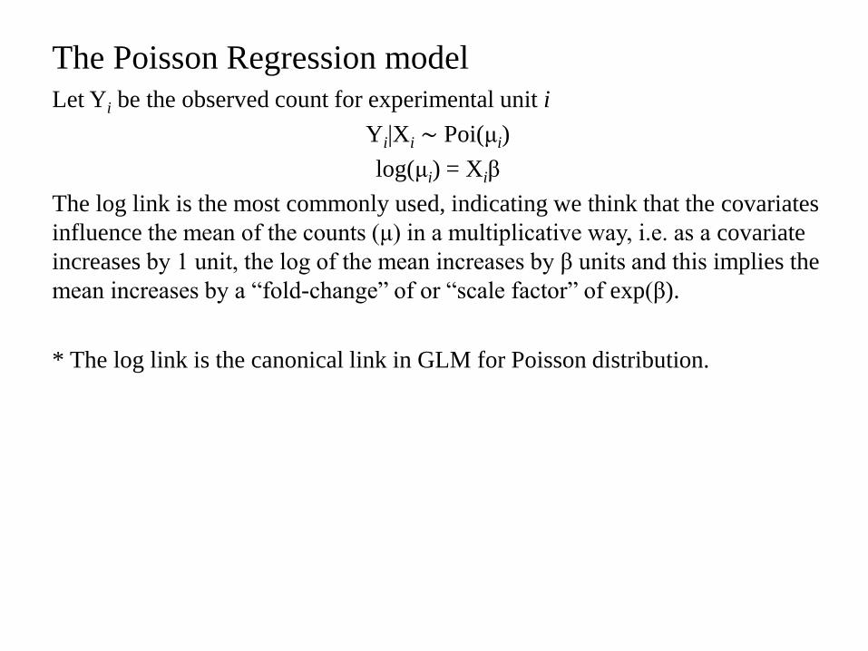
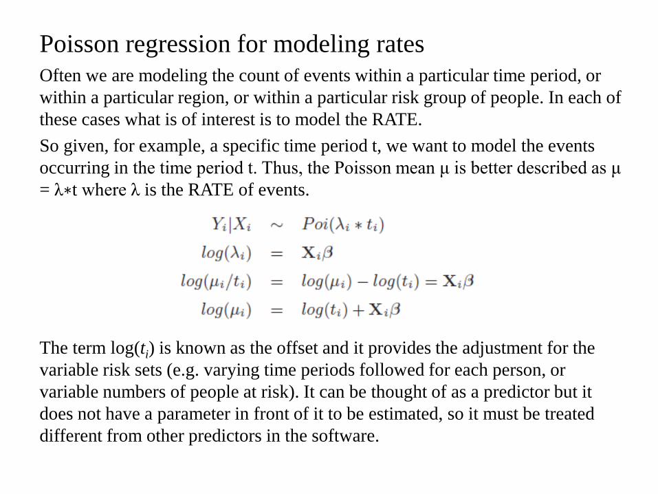
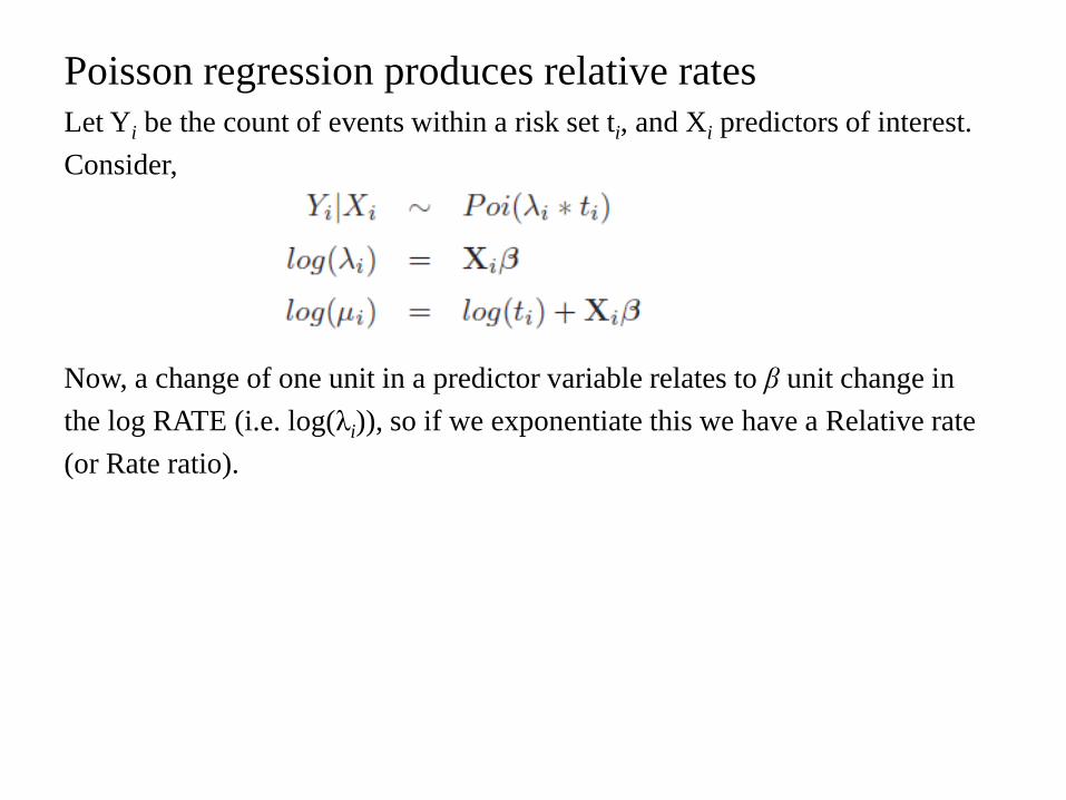
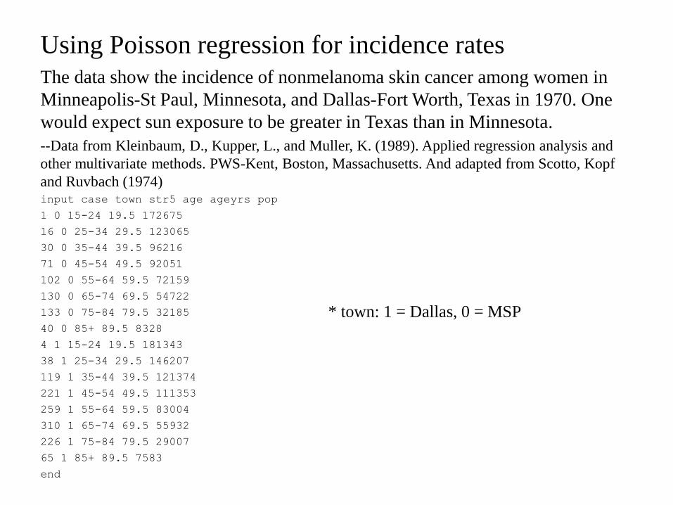
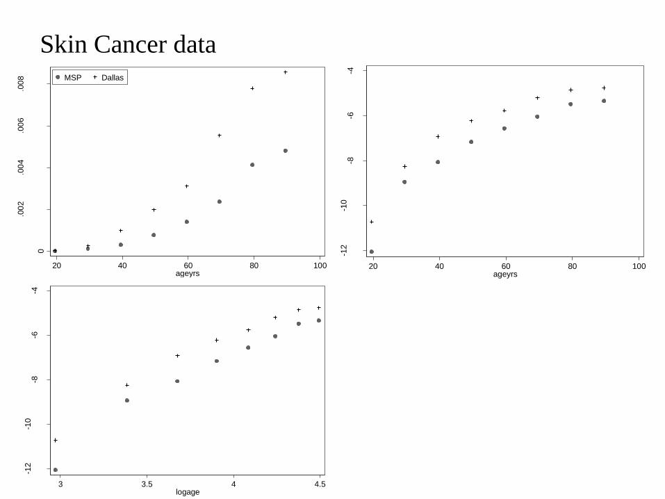
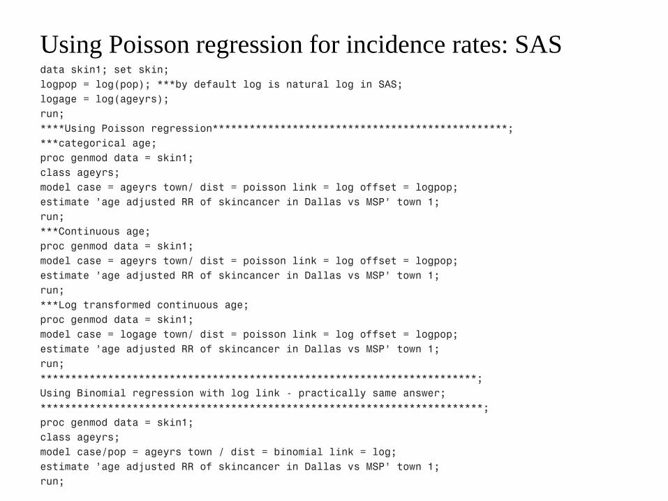
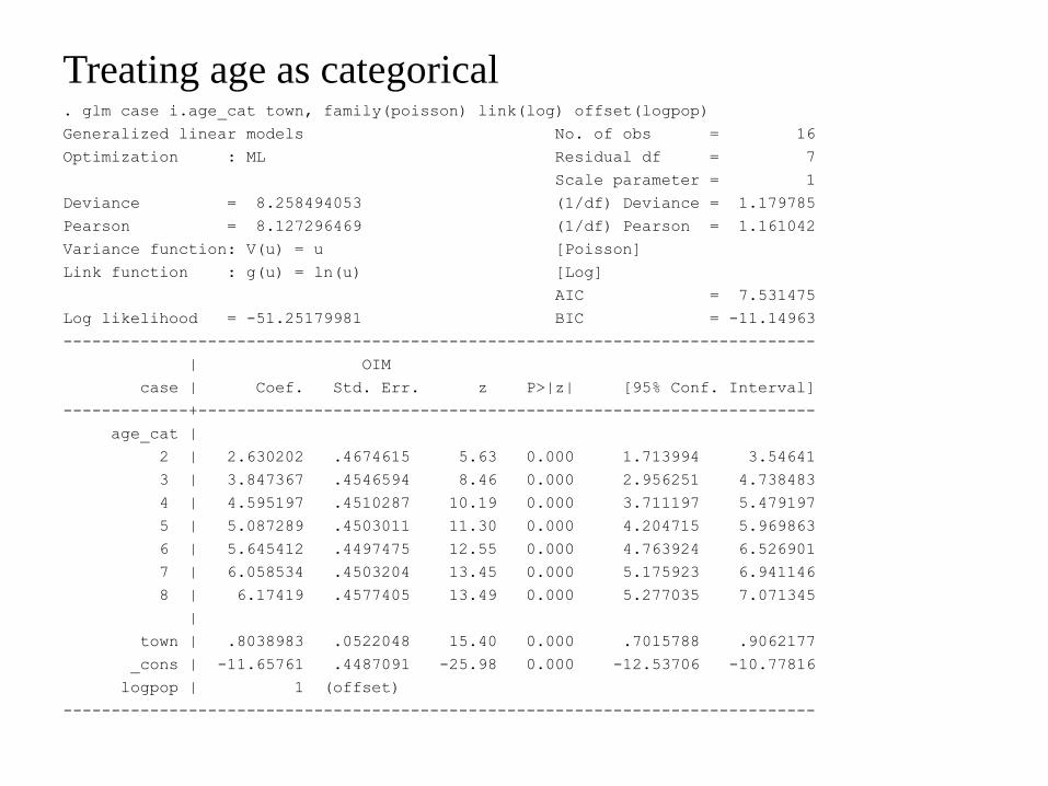
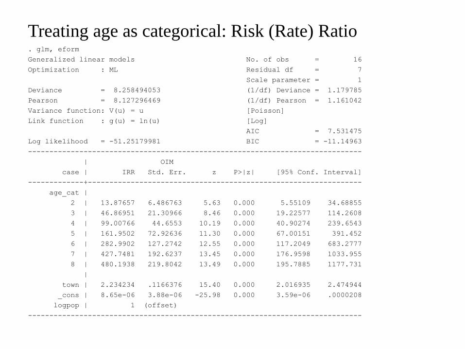
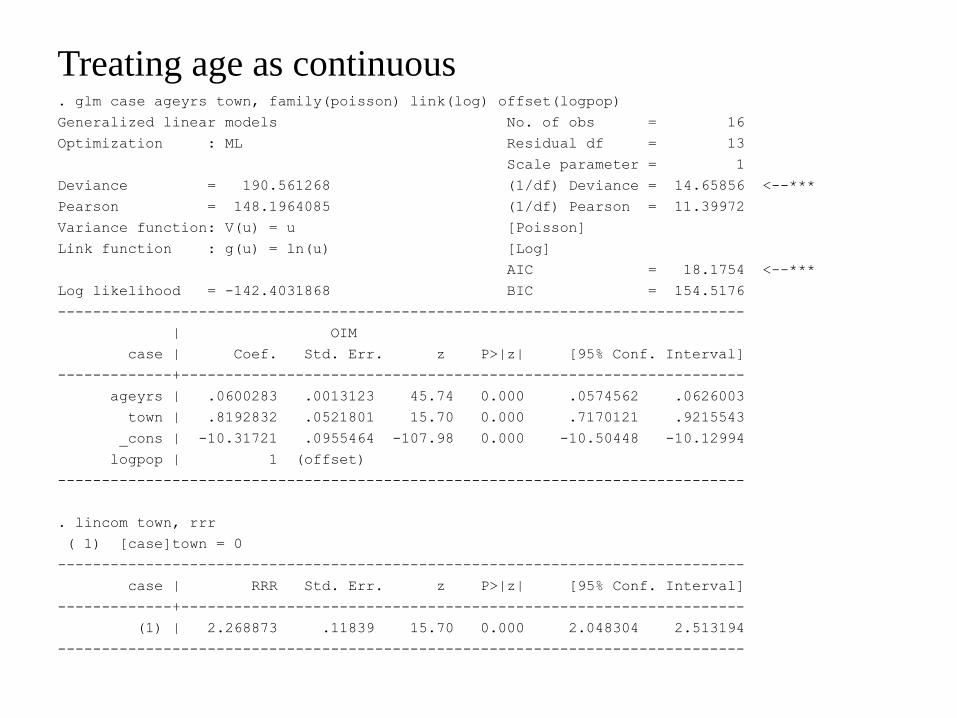
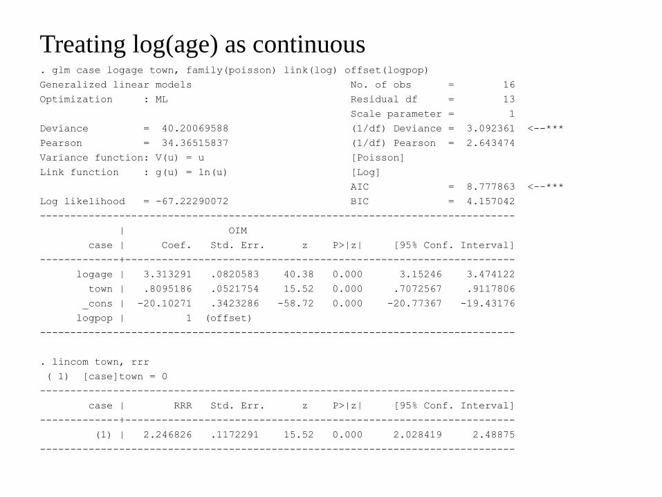
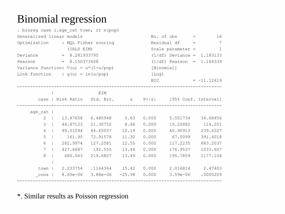
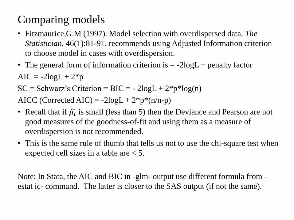
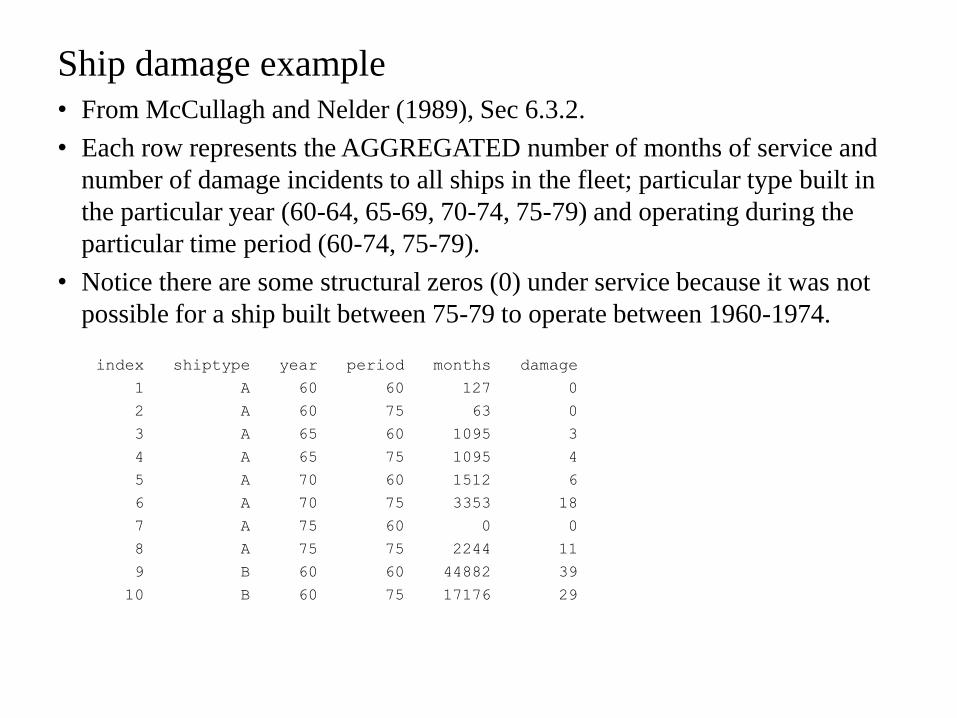
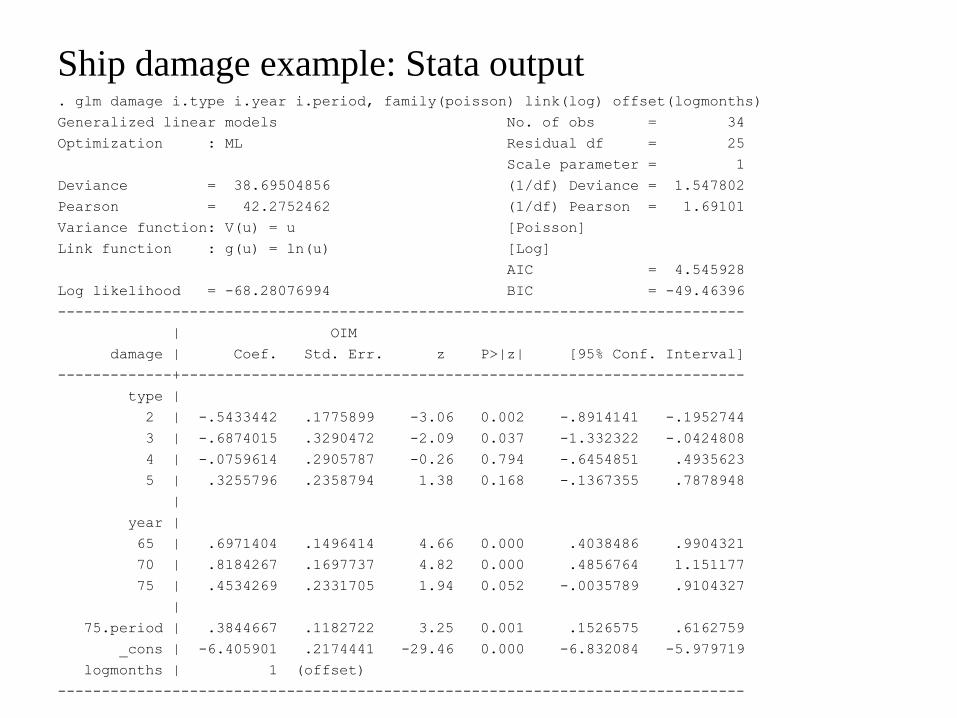
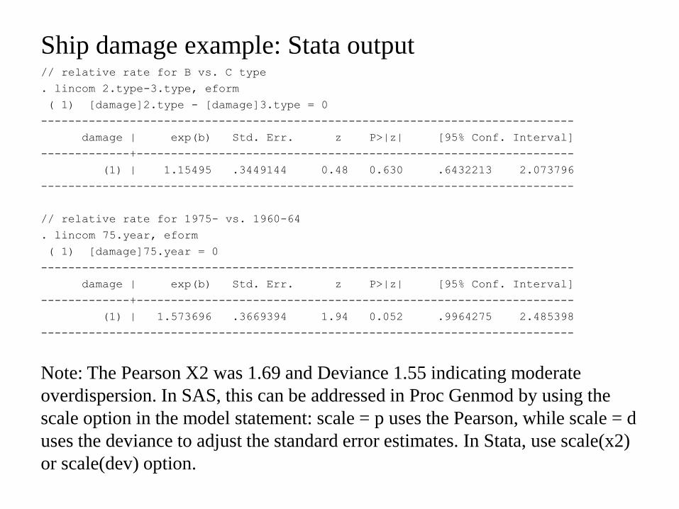
Ship damage example Stata output relative rate for B vs C type
lincom 2type-3type eform
( 1) [damage]2type - [damage]3type = 0
------------------------------------------------------------------------------
damage | exp(b) Std Err z Pgt|z| [95 Conf Interval]
-------------+----------------------------------------------------------------
(1) | 115495 3449144 048 0630 6432213 2073796
------------------------------------------------------------------------------
relative rate for 1975- vs 1960-64
lincom 75year eform
( 1) [damage]75year = 0
------------------------------------------------------------------------------
damage | exp(b) Std Err z Pgt|z| [95 Conf Interval]
-------------+----------------------------------------------------------------
(1) | 1573696 3669394 194 0052 9964275 2485398
------------------------------------------------------------------------------
Note The Pearson X2 was 169 and Deviance 155 indicating moderate
overdispersion In SAS this can be addressed in Proc Genmod by using the
scale option in the model statement scale = p uses the Pearson while scale = d
uses the deviance to adjust the standard error estimates In Stata use scale(x2)
or scale(dev) option
Ship damage example correct for overdispersion
glm damage itype iyear iperiod family(poisson) link(log) offset(logmonths) scale(x2)
------------------------------------------------------------------------------
| OIM
damage | Coef Std Err z Pgt|z| [95 Conf Interval]
-------------+----------------------------------------------------------------
type |
2 | -5433442 2309359 -235 0019 -9959702 -0907183
3 | -6874015 4278892 -161 0108 -1526049 1512459
4 | -0759614 3778651 -020 0841 -8165634 6646406
5 | 3255796 3067348 106 0288 -2756096 9267688
|
year |
65 | 6971404 1945919 358 0000 3157472 1078534
70 | 8184267 2207717 371 0000 3857221 1251131
75 | 4534269 3032122 150 0135 -1408581 1047712
|
75period | 3844667 1537997 250 0012 0830247 6859086
_cons | -6405901 2827618 -2265 0000 -6960104 -5851699
logmonths | 1 (offset)
------------------------------------------------------------------------------
(Standard errors scaled using square root of Pearson X2-based dispersion)
Ship damage example Stata output relative rate for B vs C type
lincom 2type-3type eform
( 1) [damage]2type - [damage]3type = 0
------------------------------------------------------------------------------
damage | exp(b) Std Err z Pgt|z| [95 Conf Interval]
-------------+----------------------------------------------------------------
(1) | 115495 4485226 037 0711 5395116 247244
------------------------------------------------------------------------------
relative rate for 1975- vs 1960-64
lincom 75year eform
( 1) [damage]75year = 0
------------------------------------------------------------------------------
damage | exp(b) Std Err z Pgt|z| [95 Conf Interval]
-------------+----------------------------------------------------------------
(1) | 1573696 4771638 150 0135 8686126 285112
------------------------------------------------------------------------------
Note the coefficient estimates are the same as previous output but the standard
errors and test p-values are now more conservative
Poisson regression with common risks
Previously we saw that OR and RR were quite different when the prevalence of
the risk was not small bigger than 10 In order to estimate an adjusted RR we
could use the Binomial model with a log link But sometimes there are
computational difficulties with this model An alternative is to use the Poisson
model AND to utilize the ROBUST STANDARD ERRORS Regular standard
errors for Poisson are known to be too conservative in these cases of
approximating binomial data with common risk
Binomial Regression
proc genmod data = birthwgt2 descending
class c_baseline_bmi (ref = 2) param = ref
model hibwt = totalweightgain c_baseline_bmidist=binomial link=log type3
run
Poisson Regression
proc genmod data = birthwgt2 descending
class c_baseline_bmi (ref = 2) id param = ref lt- need to generate an lsquoidrsquo variable for every sample
model hibwt = totalweightgain c_baseline_bmidist=poisson link=log type3
repeated sub = id type=ind lt- This is the statement to obtain robust std errors
run
Birthweight example log link glm hibwt totalweightgain ib2c_baseline_bmi fam(bin) link(log) eform iter(100)
Iteration 100 log likelihood = -10390036 (not concave)
convergence not achieved
AIC = 1042004
Log likelihood = -1039003635 BIC = -1310099
---------------------------------------------------------------------------------
| OIM
hibwt | Risk Ratio Std Err z Pgt|z| [95 Conf Interval]
----------------+----------------------------------------------------------------
totalweightgain | 1024364 878e-10 28e+07 0000 1024364 1024364
|
c_baseline_bmi |
1 | 0617007 0352668 -487 0000 0201262 1891555
3 | 6152626 0750599 -398 0000 4844141 7814554
4 | 1855169
|
_cons | 1368256 765e-09 -36e+07 0000 1368255 1368256
---------------------------------------------------------------------------------
Warning parameter estimates produce inadmissible mean estimates in one or
more observations
Warning convergence not achieved
Birthweight example Poisson regression with regular SE glm hibwt totalweightgain ib2c_baseline_bmi fam(poisson) link(log) eform
Generalized linear models No of obs = 2000
Optimization ML Residual df = 1995
Scale parameter = 1
Deviance = 963011489 (1df) Deviance = 4827125
Pearson = 1643646513 (1df) Pearson = 823883
Variance function V(u) = u [Poisson]
Link function g(u) = ln(u) [Log]
AIC = 7465057
Log likelihood = -7415057445 BIC = -1420079
---------------------------------------------------------------------------------
| OIM
hibwt | IRR Std Err z Pgt|z| [95 Conf Interval]
----------------+----------------------------------------------------------------
totalweightgain | 1032877 0046171 724 0000 1023868 1041966
|
c_baseline_bmi |
1 | 187722 1100813 -285 0004 0594793 5924677
3 | 1875006 3199926 368 0000 1341945 2619814
4 | 2387442 3428306 606 0000 1801783 3163466
|
_cons | 0334007 0064157 -1770 0000 022922 0486695
---------------------------------------------------------------------------------
Birthweight example Poisson regression with robust SE glm hibwt totalweightgain ib2c_baseline_bmi fam(poisson) link(log) eform robust
Generalized linear models No of obs = 2000
Optimization ML Residual df = 1995
Scale parameter = 1
Deviance = 963011489 (1df) Deviance = 4827125
Pearson = 1643646513 (1df) Pearson = 823883
Variance function V(u) = u [Poisson]
Link function g(u) = ln(u) [Log]
AIC = 7465057
Log pseudolikelihood = -7415057445 BIC = -1420079
---------------------------------------------------------------------------------
| Robust
hibwt | IRR Std Err z Pgt|z| [95 Conf Interval]
----------------+----------------------------------------------------------------
totalweightgain | 1032877 0038243 874 0000 1025409 10404
|
c_baseline_bmi |
1 | 187722 1077046 -292 0004 0609737 5779468
3 | 1875006 2884014 409 0000 1386999 2534714
4 | 2387442 3093241 672 0000 1852032 3077634
|
_cons | 0334007 005491 -2068 0000 0242002 0460989
---------------------------------------------------------------------------------
Other count models
bull Zero-truncated Poisson
Example A study by the county traffic court on the number of tickets
received by teenagers as predicted by school performance amount of driver
training and gender Only individuals who have received at least one
citation are in the traffic court files
SAS proc nlmixed
(httpwwwatsuclaedustatsasfaqzt_nlmixedhtm)
Stata tpoisson y x1 x2 inflate(x1)
(httpwwwatsuclaedustatsasfaqzt_nlmixedhtm)
Other count models
bull Zero-inflated Poisson
Example The state wildlife biologists want to model how many fish are
being caught by fishermen at a state park Visitors are asked whether or not
they have a camper how many people were in the group were there
children in the group and how many fish were caught Some visitors do not
fish but there is no data on whether a person fished or not Some visitors
who did fish did not catch any fish so there are excess zeros in the data
because of the people that did not fish
SAS proc genmod data = hellip model y = x1 x2 dist=zip zeromodel x1 link = logit
(httpwwwatsuclaedustatsasdaezipreghtm)
Stata zip y x1 x2 inflate(x1)
(httpwwwatsuclaedustatstatadaeziphtm)
Other count models
bull Negative binomial model
ndash Have one more parameter than the Poisson the second parameter can be
used to adjust the variance independently of the mean
ndash Alternative solution to overdispersed Poisson
SAS proc genmod data = hellip model y = x1 x2 dist=negbin
Stata glm y x1 x2 family(nb)
bull Zero-inflated negative binomial model
bull Zero-truncated negative binomial model
( Check the UCLA website for examples)
Estimation and Goodness of fit for GLM
bull Estimation
ndash MLE maximize the log-likelihood
ndash Iterated Weighted Least Squares (IWLS) analogous to weighted least
squares with the weights updated iteratively
GLM fits using IWLS is more general than MLE (see eg quasi-likelihood
if you want to know more details)
bull Goodness of fit
ndash Pearsonrsquos X2 (does not depend on distribution assumption)
where mi = 1 for Normal and Poisson ni for Binomial
ndash Deviance (does not depend on ϕ but depends on log-likelihood)
where (natural parameter for the saturated model)
2
2
1
ˆ
ˆ
ni i
i i i
YX
V m
1
ˆ ˆ 2
ˆ ˆ2n
i i i i i i
i
D Y l Y Y l Y
m Y b b
i ib Y
Residuals bull Types of Residuals
ndash Pearson residual
ndash Deviance residual
ndash Response residual
ndash Working residual
ndash Partial residual
Note residual diagnostics non-informative for binary data
bull Overdispersion Var(Y) gt a(ϕ)V(μ) for any GLM
check if X2(n-p) or D(n-p) gtgt 1
ˆ
ˆ
P i ii
i
Yr
V
ˆD
i i i ir sign Y d
ˆ
ˆˆ
W ii i i
i
r Y
ˆR
i i ir Y
ˆ ˆˆˆ
T iki i i ik k
i
r Y x
Checking outliers
Check for observations with large (standardized) Pearson or deviance
residuals
Deviance residual is generally preferred to the Pearson residual since its
distributional properties are closer to the residuals in linear regression
-2-1
01
2
sta
nda
rdiz
ed
de
via
nce
re
sid
ua
l
0 100 200 300predicted mean case
-2-1
01
2
sta
nda
rdiz
ed
Pe
ars
on
re
sid
ua
l
0 100 200 300predicted mean case
Checking the variance function
The x-axis is ldquoconstant-information scalerdquo for Poisson errors See McCullagh
and Nelder ldquoGeneralized Linear Modelsrdquo (Chapter 1261)
Positive trend indicates the current variance function increases too slowly with
the mean
05
11
52
abso
lute
sta
nda
rdiz
ed d
evia
nce
resid
ual
0 10 20 30 402sqrt(mu)
Checking for linearity lowess plot
Other approach to check departure from linearity
ndash Add polynomial terms (eg age^2) and test for their statistical
significance
ndash Group continuous predictor into categories (eg age_cat)
-26
-24
-22
-2-1
8-1
6
low
ess h
ibw
t ag
e_lm
p
15 20 25 30 35 40age_lmp
Other Diagnostics
bull Checking the link function the simplest method is to include as
covariate and assessing the fall in deviance (Hinkley 1985)
bull Partial residual is helpful to assess the form of covariates ie plot partial
residual against the corresponding predictor
bull Checking influential points modified Cookrsquos distance (gt 4(n-p) to be
problematic)
2
02
46
81
Coo
ks
dis
tan
ce
0 5 10 15observation
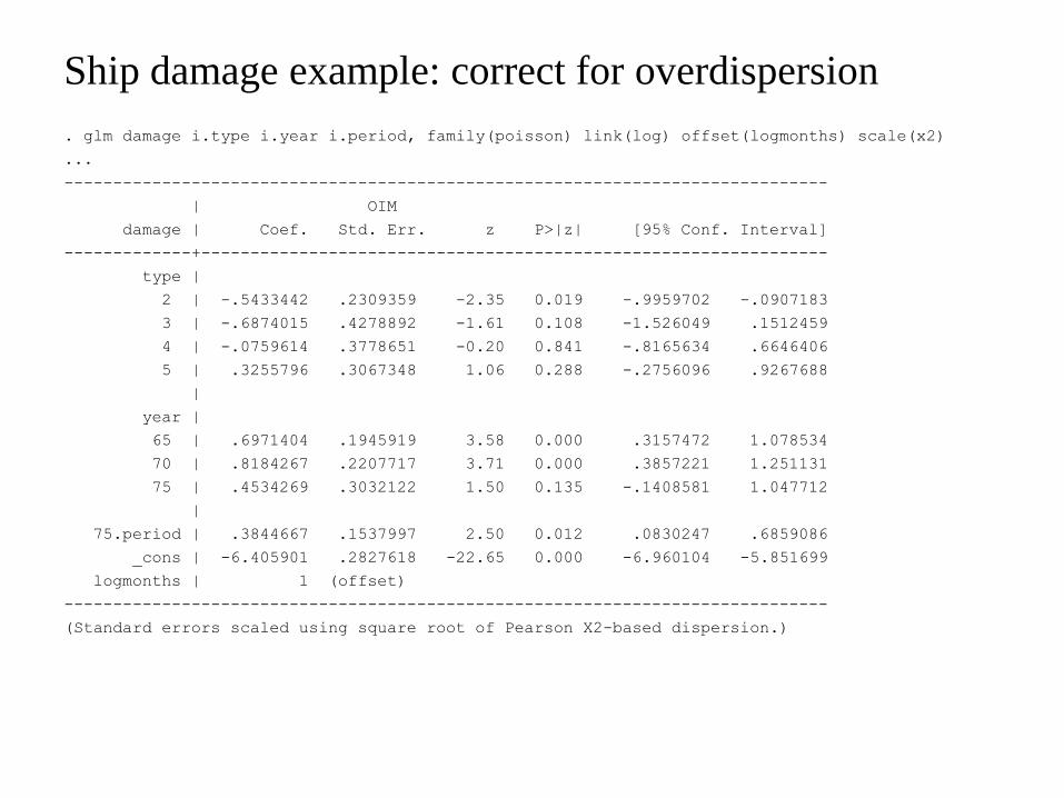
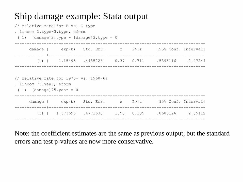
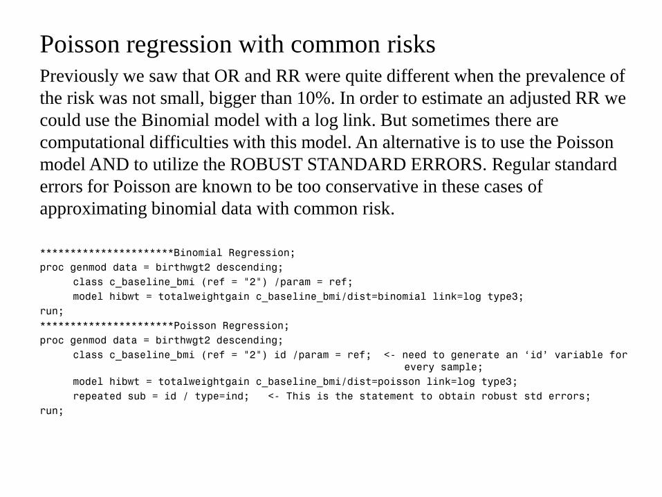
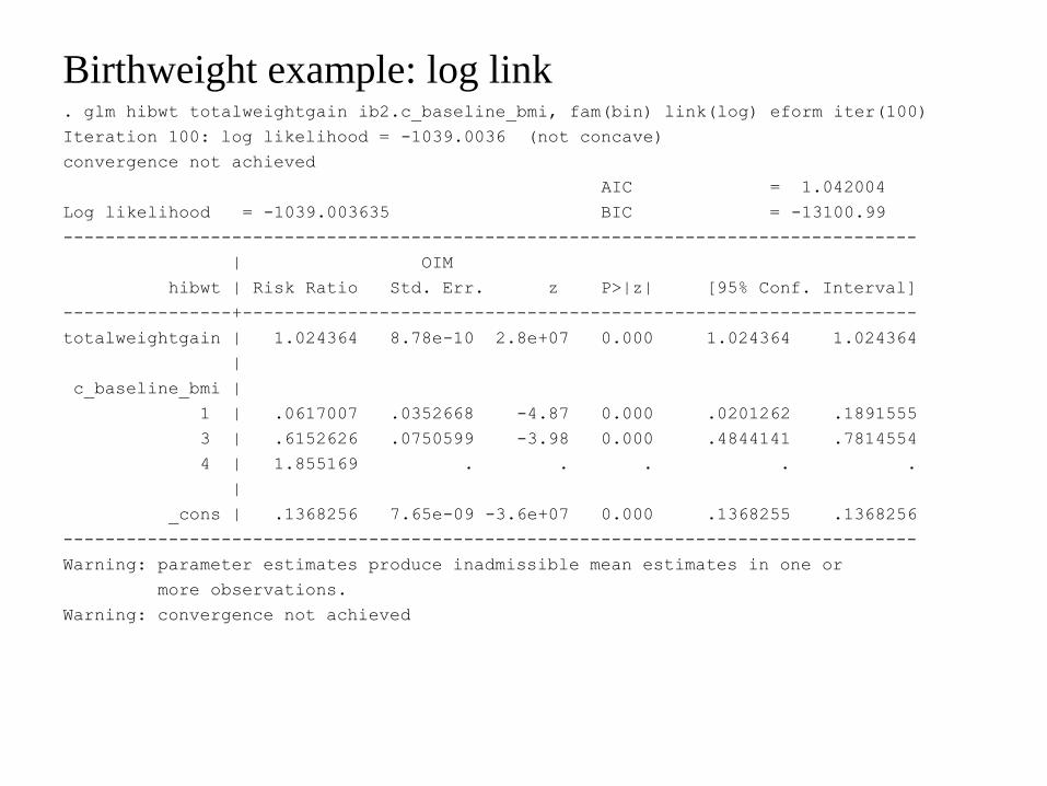
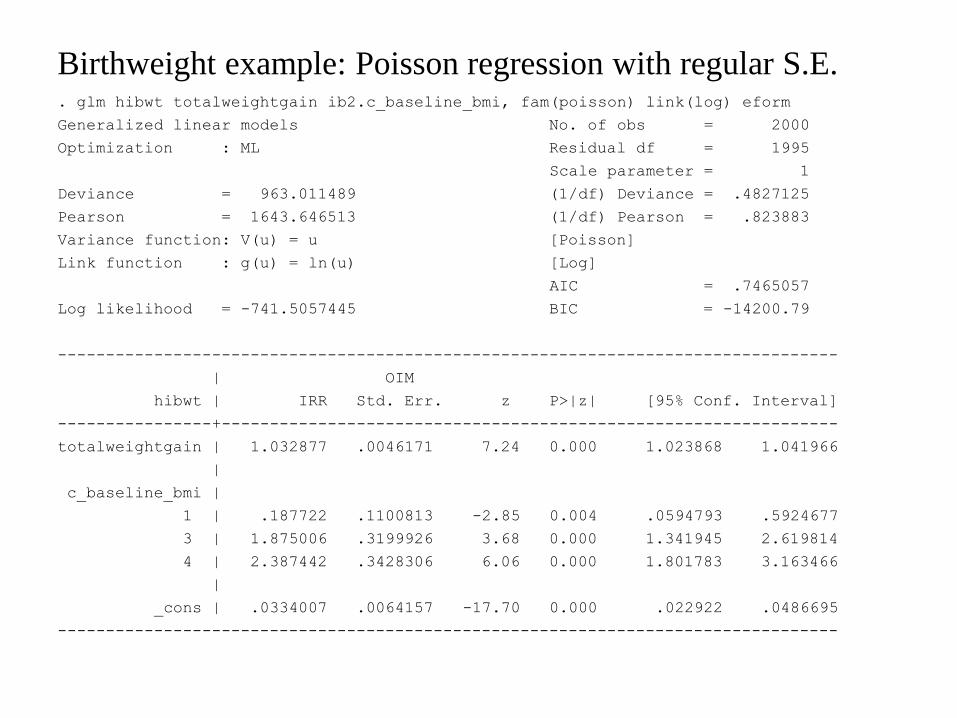
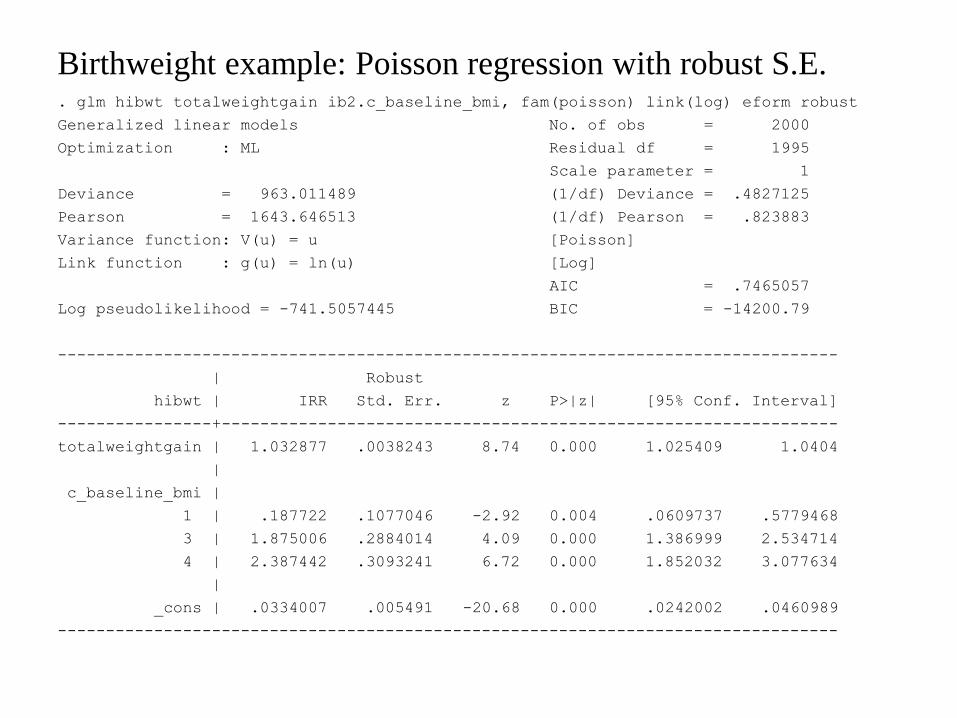
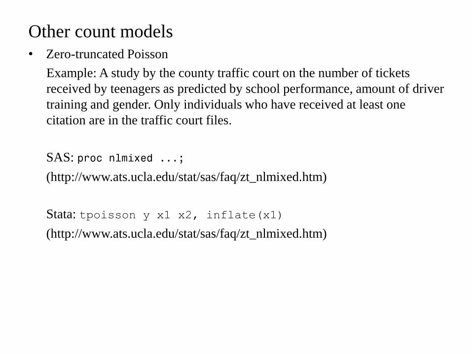
Other count models
bull Zero-inflated Poisson
Example The state wildlife biologists want to model how many fish are
being caught by fishermen at a state park Visitors are asked whether or not
they have a camper how many people were in the group were there
children in the group and how many fish were caught Some visitors do not
fish but there is no data on whether a person fished or not Some visitors
who did fish did not catch any fish so there are excess zeros in the data
because of the people that did not fish
SAS proc genmod data = hellip model y = x1 x2 dist=zip zeromodel x1 link = logit
(httpwwwatsuclaedustatsasdaezipreghtm)
Stata zip y x1 x2 inflate(x1)
(httpwwwatsuclaedustatstatadaeziphtm)
Other count models
bull Negative binomial model
ndash Have one more parameter than the Poisson the second parameter can be
used to adjust the variance independently of the mean
ndash Alternative solution to overdispersed Poisson
SAS proc genmod data = hellip model y = x1 x2 dist=negbin
Stata glm y x1 x2 family(nb)
bull Zero-inflated negative binomial model
bull Zero-truncated negative binomial model
( Check the UCLA website for examples)
Estimation and Goodness of fit for GLM
bull Estimation
ndash MLE maximize the log-likelihood
ndash Iterated Weighted Least Squares (IWLS) analogous to weighted least
squares with the weights updated iteratively
GLM fits using IWLS is more general than MLE (see eg quasi-likelihood
if you want to know more details)
bull Goodness of fit
ndash Pearsonrsquos X2 (does not depend on distribution assumption)
where mi = 1 for Normal and Poisson ni for Binomial
ndash Deviance (does not depend on ϕ but depends on log-likelihood)
where (natural parameter for the saturated model)
2
2
1
ˆ
ˆ
ni i
i i i
YX
V m
1
ˆ ˆ 2
ˆ ˆ2n
i i i i i i
i
D Y l Y Y l Y
m Y b b
i ib Y
Residuals bull Types of Residuals
ndash Pearson residual
ndash Deviance residual
ndash Response residual
ndash Working residual
ndash Partial residual
Note residual diagnostics non-informative for binary data
bull Overdispersion Var(Y) gt a(ϕ)V(μ) for any GLM
check if X2(n-p) or D(n-p) gtgt 1
ˆ
ˆ
P i ii
i
Yr
V
ˆD
i i i ir sign Y d
ˆ
ˆˆ
W ii i i
i
r Y
ˆR
i i ir Y
ˆ ˆˆˆ
T iki i i ik k
i
r Y x
Checking outliers
Check for observations with large (standardized) Pearson or deviance
residuals
Deviance residual is generally preferred to the Pearson residual since its
distributional properties are closer to the residuals in linear regression
-2-1
01
2
sta
nda
rdiz
ed
de
via
nce
re
sid
ua
l
0 100 200 300predicted mean case
-2-1
01
2
sta
nda
rdiz
ed
Pe
ars
on
re
sid
ua
l
0 100 200 300predicted mean case
Checking the variance function
The x-axis is ldquoconstant-information scalerdquo for Poisson errors See McCullagh
and Nelder ldquoGeneralized Linear Modelsrdquo (Chapter 1261)
Positive trend indicates the current variance function increases too slowly with
the mean
05
11
52
abso
lute
sta
nda
rdiz
ed d
evia
nce
resid
ual
0 10 20 30 402sqrt(mu)
Checking for linearity lowess plot
Other approach to check departure from linearity
ndash Add polynomial terms (eg age^2) and test for their statistical
significance
ndash Group continuous predictor into categories (eg age_cat)
-26
-24
-22
-2-1
8-1
6
low
ess h
ibw
t ag
e_lm
p
15 20 25 30 35 40age_lmp
Other Diagnostics
bull Checking the link function the simplest method is to include as
covariate and assessing the fall in deviance (Hinkley 1985)
bull Partial residual is helpful to assess the form of covariates ie plot partial
residual against the corresponding predictor
bull Checking influential points modified Cookrsquos distance (gt 4(n-p) to be
problematic)
2
02
46
81
Coo
ks
dis
tan
ce
0 5 10 15observation
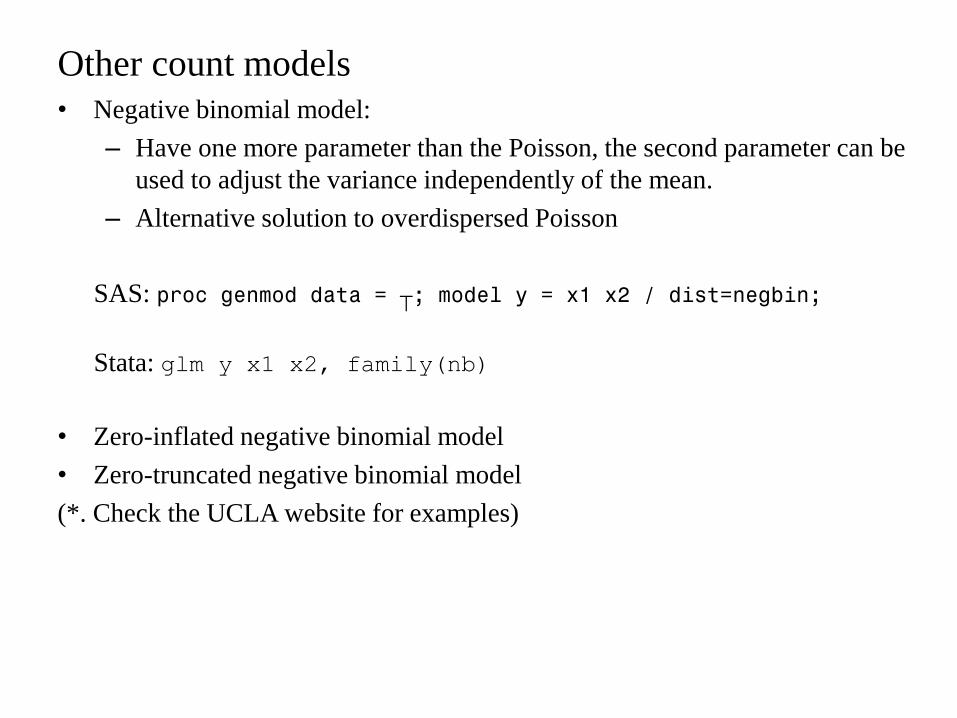
Other count models
bull Negative binomial model
ndash Have one more parameter than the Poisson the second parameter can be
used to adjust the variance independently of the mean
ndash Alternative solution to overdispersed Poisson
SAS proc genmod data = hellip model y = x1 x2 dist=negbin
Stata glm y x1 x2 family(nb)
bull Zero-inflated negative binomial model
bull Zero-truncated negative binomial model
( Check the UCLA website for examples)
Estimation and Goodness of fit for GLM
bull Estimation
ndash MLE maximize the log-likelihood
ndash Iterated Weighted Least Squares (IWLS) analogous to weighted least
squares with the weights updated iteratively
GLM fits using IWLS is more general than MLE (see eg quasi-likelihood
if you want to know more details)
bull Goodness of fit
ndash Pearsonrsquos X2 (does not depend on distribution assumption)
where mi = 1 for Normal and Poisson ni for Binomial
ndash Deviance (does not depend on ϕ but depends on log-likelihood)
where (natural parameter for the saturated model)
2
2
1
ˆ
ˆ
ni i
i i i
YX
V m
1
ˆ ˆ 2
ˆ ˆ2n
i i i i i i
i
D Y l Y Y l Y
m Y b b
i ib Y
Residuals bull Types of Residuals
ndash Pearson residual
ndash Deviance residual
ndash Response residual
ndash Working residual
ndash Partial residual
Note residual diagnostics non-informative for binary data
bull Overdispersion Var(Y) gt a(ϕ)V(μ) for any GLM
check if X2(n-p) or D(n-p) gtgt 1
ˆ
ˆ
P i ii
i
Yr
V
ˆD
i i i ir sign Y d
ˆ
ˆˆ
W ii i i
i
r Y
ˆR
i i ir Y
ˆ ˆˆˆ
T iki i i ik k
i
r Y x
Checking outliers
Check for observations with large (standardized) Pearson or deviance
residuals
Deviance residual is generally preferred to the Pearson residual since its
distributional properties are closer to the residuals in linear regression
-2-1
01
2
sta
nda
rdiz
ed
de
via
nce
re
sid
ua
l
0 100 200 300predicted mean case
-2-1
01
2
sta
nda
rdiz
ed
Pe
ars
on
re
sid
ua
l
0 100 200 300predicted mean case
Checking the variance function
The x-axis is ldquoconstant-information scalerdquo for Poisson errors See McCullagh
and Nelder ldquoGeneralized Linear Modelsrdquo (Chapter 1261)
Positive trend indicates the current variance function increases too slowly with
the mean
05
11
52
abso
lute
sta
nda
rdiz
ed d
evia
nce
resid
ual
0 10 20 30 402sqrt(mu)
Checking for linearity lowess plot
Other approach to check departure from linearity
ndash Add polynomial terms (eg age^2) and test for their statistical
significance
ndash Group continuous predictor into categories (eg age_cat)
-26
-24
-22
-2-1
8-1
6
low
ess h
ibw
t ag
e_lm
p
15 20 25 30 35 40age_lmp
Other Diagnostics
bull Checking the link function the simplest method is to include as
covariate and assessing the fall in deviance (Hinkley 1985)
bull Partial residual is helpful to assess the form of covariates ie plot partial
residual against the corresponding predictor
bull Checking influential points modified Cookrsquos distance (gt 4(n-p) to be
problematic)
2
02
46
81
Coo
ks
dis
tan
ce
0 5 10 15observation
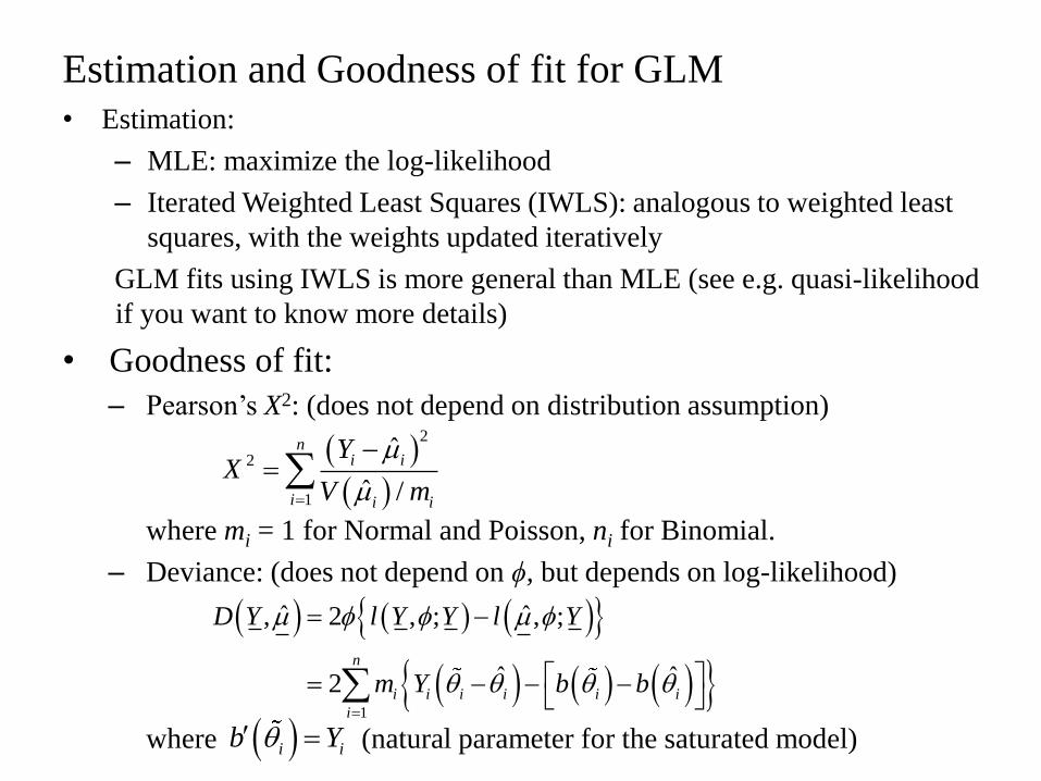
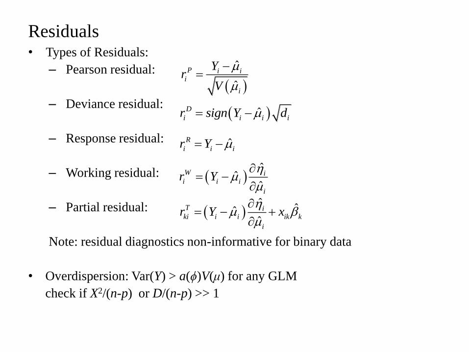
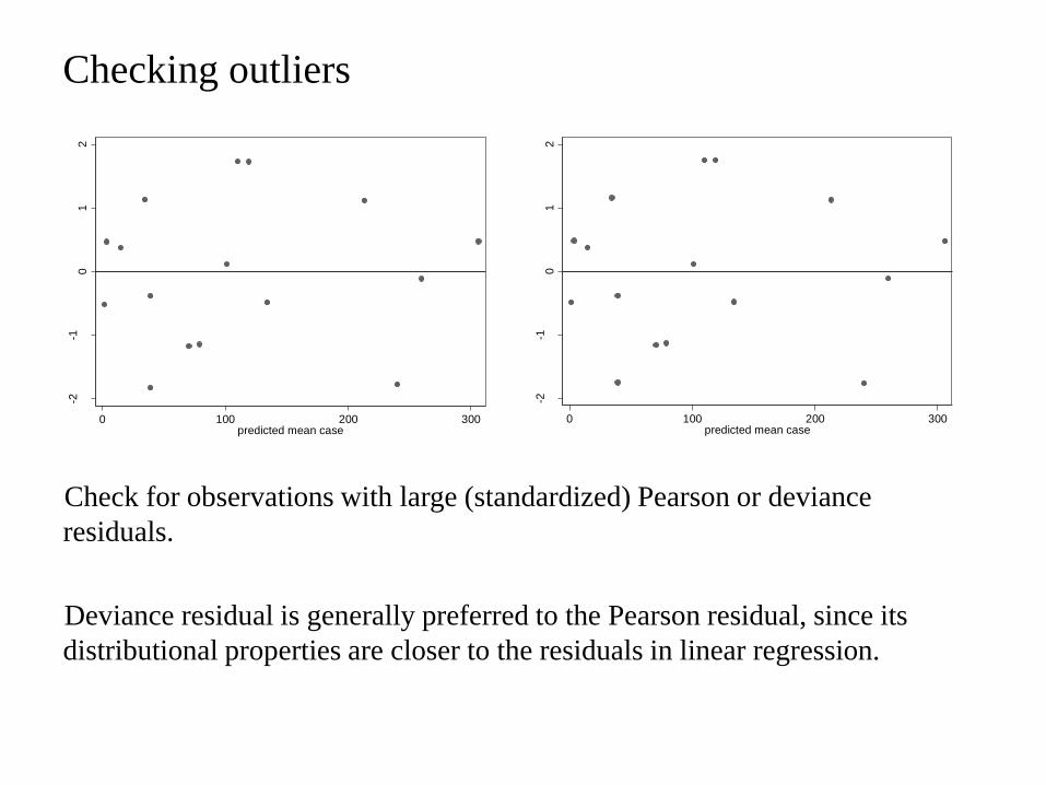
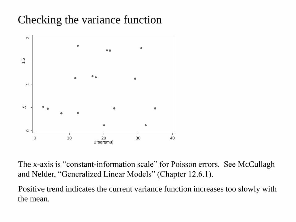
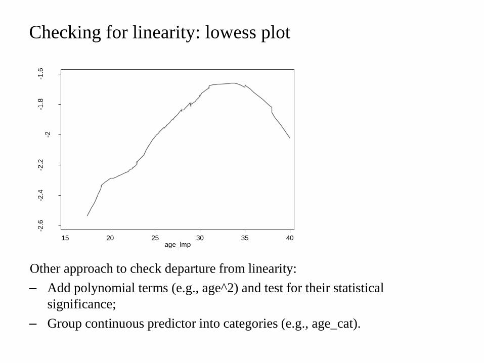
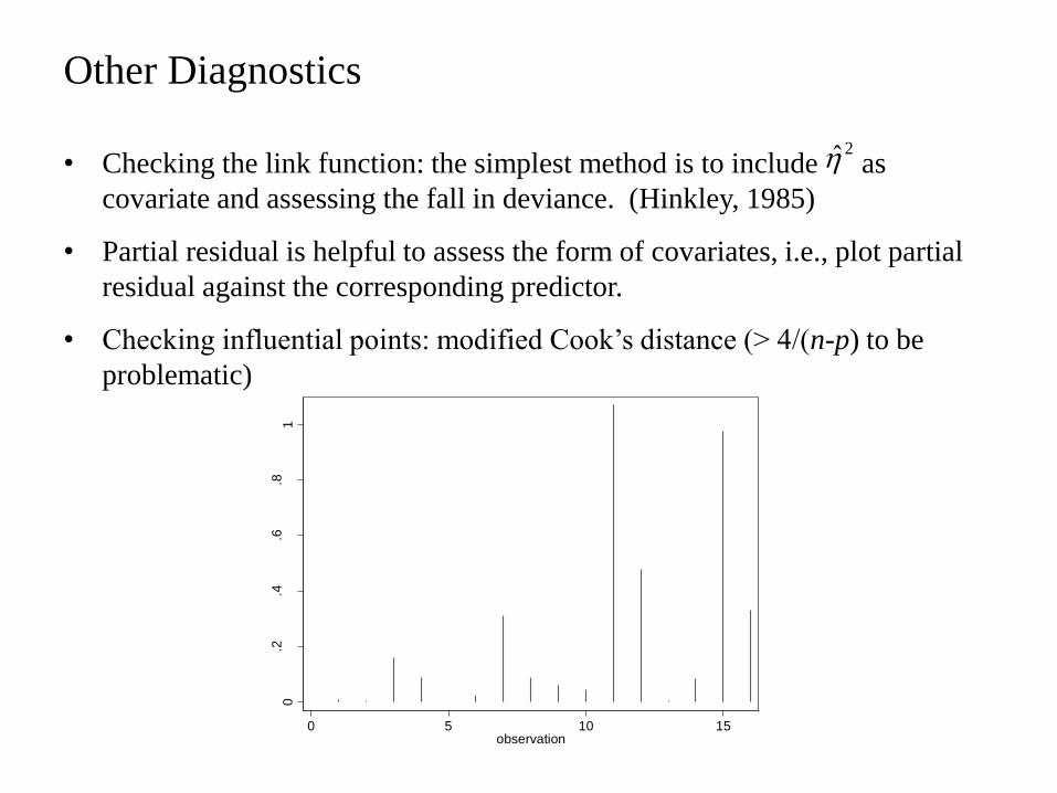