A primer on rating agencies as monitors:an analysis of the watchlist period

This version: November 16, 2007

Abstract

In much of the literature, rating agencies are seen as institutions providing infor-mational services to the market. Our paper contributes to this literature by lookingclosely at the watchlist period, a particularly well-defined monitoring event. Weare interested in the evolution of default risk expectations over the watchlist pe-riod. The change in the firm’s distance to default, relative to a benchmark groupof firms, serves as our metric of market expectations. Using a complete data set ofMoody’s watchlist operations since 1991, we find that sorting of firms by abnormalchange in distance to default only partially explains the rating decision. Relying ona clean sample of watchlist initiations with no prior, we find a significant abnormalreturn which can be explained by proxies for the agency cost of debt. Since marketexpectations rely on publicly available information, we conclude that private infor-mation plays a role in the eventual rating assignment. Our results provide indirectevidence for an active monitoring role of rating agencies, as recently suggested byBoot, Milbourn, and Schmeits (2006).

Keywords: Credit Rating Agencies; Watchlist; Distance to Default; Rating Ac-tions; Event Study

JEL: G33, G14, G29

1 Introduction

What is the relevance of rating agencies in today’s capital markets? Assessments by the

popular press diverge widely. For some observers, rating agencies are notoriously slow

and unreliable producers of information. They have a poor record of crisis forecasting,

as evidenced by the Asian crisis,1 and by many prominent credit events, e.g. Enron and

Worldcom.2 In line with a weak forecasting record, most empirical studies on rating action

and stock market return find rather limited effects of rating announcements on a firms

market values. More specifically, most studies find limited share price effects for down-

grades, and typically no effect for upgrades (see Hand, Holthausen, and Leftwich (1992);

Cantor (2004) for a survey).

For a different group of observers, rating agencies play a rather influential role in

today’s markets. In Friedman (2005) rating agencies stand out in their impact on market

valuation, through their rating decisions. In particular, downgrade decisions are some-

times seen as “verdicts” that exert a profound influence on a firm’s refinancing costs. In

the aftermath of the Enron debacle, Joe Lieberman, then-Chairman of the US Senate

Committee on Governmental Affairs stated on March 20, 2002: “Someone once said that

raters hold “almost biblical authority”. On a NewsHour with Jim Lehrer program in 1996,

New York Times columnist Tom Friedman went so far as to say - and I quote - “there

are two superpowers in the world... the United States and Moody’s Bond Rating Service...

and believe me, it’s not clear sometimes who is more powerful”.”3 For some observers,

therefore, rating agencies are perceived as being opaque, oligopolistic, and powerful.

We contribute to this debate by providing evidence in support of a third, and more

balanced view: rating agencies are monitors in the sense of standard setters, affecting

company valuation and company default risk in the interest of bondholder wealth. An

example of what we have in mind is provided by the case of Constellation Brands Inc., a

U.S. wine producer and distributor. The NYSE listed company announced its intention

1See e.g. on Banking Supervision (1998).2See Moody’sKMV (2007) for a comparison of the Moody’s KMV and the S&P Rating.3See Lieberman (2002).

1

to take over BRL Hardy Ltd., Australia’s largest wine producer. On February 23, 2003

it released a press statement: “Constellation Brands Inc. also announced that Moody’s

Investors Service confirmed the Company’s rating on its existing debt and assigned a

higher rating of BA1 to the Company’s new bank facility. The credit rating is predicated

on Constellation issuing sufficient equity in connection with the transaction and after

closing to reduce its debt. Moody’s previously put Constellation on credit watch following

the announcement of the Company’s $1.4 billion acquisition of BRL Hardy.”4

In such a setting, we can study how the announcement of a monitoring process in-

fluences a proxy of the firm’s default risk, as it is seen by the market. While we do not

observe the individual decisions taken by the firm during the monitoring periods, we can

learn about them in the time series of default risk expectations. More precisely, we bench-

mark these expectations by referring to a group of firms in the same rating notch as the

monitored firm that do not have an ongoing watchlist event. We then use a difference-in-

difference approach to identify the marginal impact of the agency on market expectations

of firm default risk.

As a measure of the market expectations of a firm’s default risk we use the abnormal

distance to default (ADD). To arrive at the ADD, we first calculate the distance to default

borrowing from recent work by Vassalou and Xing (2004). We then substract the mean

value of a peer group of firms belonging to the same rating class to arrive at the ADD.

The measure reflects changes in the share price, its volatility, and the firm’s leverage. It

is, therefore, well suited for modelling the real consequences of rating agency behavior.

Since our measure is non-standard in the literature, we also check the accuracy of our risk

proxy by testing both specification and power of our measure, applying a test suggested

by Barber and Lyon (1996).

Our main findings can be summarized as follows: first, over the full sample period

(October 1991 to December 2004), at the time of watchlist announcement, default risk

expected by the market tends to rise, relative to the peer group. There is an insignificant

difference in the jump in default risk expectation between the two subgroups: those firms

4See PRNewswire (2003).

2

that later on will be downgraded, and those that will see their original rating confirmed,

suggesting the market to efficiently reflect available information.

Second, we look at the monitoring period, which we define to extend from day +3

after the initial watchlist announcement until day -3 before the final rating decision. Over

the monitoring subperiod, ADD differs between the two subgroups: e.g., it decreases for

the ‘confirmation’ subsample, while it does not decrease for the ‘downgrade’ subsample,

suggesting that firms sort themselves into two subgroups. Sorting is due to observable

actions taken by the firms, since the measure of performance we use is the abnormal

change in implied distance to default.

Third, sorting alone does not explain the eventual rating decision. Upon announce-

ment of the final rating decision, the ADD proxy decreases strongly for the downgrade

subsample, whereas it remains constant for the confirmation group. Note, that over the

entire watchlist period, including the initial event, the confirmation group experiences a

zero change in expected default risk.

Finally, for the full sample of firms without designated direction , i.e. when the de-

clared designation is ’uncertain’, rather than upgrade or downgrade, we find no significant

ADD around watchlist announcement. When decomposing the effect, we find that return

and risk are both rising around watchlist announcement, consistent with a positive effect

of agency monitoring on company expected return. This sample, however, is affected by

confounding events, like M&A deal announcements.

In order to alleviate the effect of confounding events, particularly the impact of M&A

activities, we then construct a sample free of any directional prior expectations. This

sample consists of all ”uncertain watchlist additions” for which we cannot identify any

trigger event. Presumably, these cases were genuine surprises in the eyes of market par-

ticipants. Thus, the announcement effect of watchlist additions will correspond to the net

shareholder wealth effect of a watchlist addition. Our ’clean’ data set yields a small, but

significantly positive shareholder wealth effect.

We also try to explain the magnitude of this wealth effect and find once again support

3

for a positive, agency cost-reducing role of watchlist initiation. A cross sectional analysis

reveals that cumulative abnormal returns around watchlist announcement depend upon

proxies for the level of bondholder-shareholder conflicts.

Overall, our findings support the idea of an active consultation process between firms

and the rating agency during watchlist period. Over time, the market learns about the

consultation process, and whether or not the firm adjusts its financing policy, or alters its

asset structure. Particularly for downgrade designations, stock prices reflect a lowering of

default risk expectations, signaling early on when a company is drifting towards rating

confirmation.

Furthermore, at termination of the watchlist, when the actual rating decision is an-

nounced, downgraded firms experience a further jump of their default risk estimate (ADD

proxy). This is analogous to the expiration of an option. As long as the watchlist-cum-

monitoring period is ongoing, there is always some hope that the firm can fulfill the

standards set by the agency. At watchlist termination, this option expires. The down-

grade decision signals to the market that, according to the rating agency, there is no

further room for default risk improvement. Without the option, debt valuation will drop,

and distance to default will rise.

Our approach contributes to the question, recently raised by Boot, Milbourn, and

Schmeits (2006), of whether rating agencies influence firm financing decisions through

their standard setting and monitoring process.

Our analysis is interesting for another reason. The watchlist period is an ideal and

hitherto unexplored institutional phenomenon that allows us to study the effect of mon-

itoring on the behavior of the client.5 The period we are studying is special because it

provides us with time-stamped data of initiation and termination of the monitoring pro-

cess. In contrast, information on the effect of bank monitoring on borrower behavior is

typically less precise. Furthermore, all events we are studying are public information, and

5Direct upgrades or downgrades, i.e. rating action without a preceding watchlist period, may also

involve rating investigations by the agency. However, in these cases the exact initiation date is not made

public and, therefore, market response to agency activities cannot be easily identified.

4

market reactions can be observed on a daily basis.

The remainder of the paper is organized as follows. We review the related literature

in Section 2 and provide some background on the watchlist in Section 3. In Section 4 we

discuss the abnormal distance to default. We develop our hypotheses in Section 5, present

data and summary statistics in Section 6, and present our results in Section 7. Finally,

Section 8 concludes.

2 Related Literature

The watchlist and its role in the rating process have been largely neglected to date. There

are two exceptions. Boot, Milbourn, and Schmeits (2006) propose a theoretical model,

where the watchlist period allows the bondmarket to settle in a rational expectations

equilibrium in which firms can recover their credit quality after an initial drop in firm

quality. Hand, Holthausen, and Leftwich (1992) analyze the abnormal return surrounding

rating changes as well as watchlist additions. Their study relies on a sample of S&P’s

Credit Watch, with 253 observation (38 upgrades) in the 1981-1983 period. They find

negative abnormal announcement returns for those firms that were classified by an ex-

pectations model as being placed on Credit Watch unexpectedly. However, in the Hand,

Holthausen, and Leftwich (1992) study, the authors do not track the Credit Watch addi-

tions all the way through to the watchlist resolution, as does our study.

Our model of the market assessment of credit risk draws on the structural model of

Merton (1974). Odgen (1987) and Jones, Mason, and Rosenfeld (1984) study the pre-

dictability of bond prices using an empirical version of the Merton (1974) model. Eom,

Helwege, and Huang (2004) and Lyden and Saraniti (2001) compare the performance of

different structural models in forecasting bond prices, while Tarashev (2005) compares

structural models and agency ratings.

Our analysis is also related to the literature comparing the performance of different

credit risk models. For example, Hillegeist, Keating, Cram, and Lundstedt (2004) compare

default probabilities estimated from the Merton (1974) model with Altman’s Z score,

5

while Delianedis and Geske (2003) and Du and Suo (2003) compare agency ratings and

structural models. Robbe and Mahieu (2005) study the ability to forecast rating changes

using the KMV model, and Vassalou and Xing (2005) analyze the estimates from the

Merton (1974) model around rating changes.

Our study provides new evidence in several respects. First, it looks in detail at the

‘inner’ watchlist period, aside from watchlist entry and exit. Furthermore, it tracks the

distance to default as a way to retrieve concurrent market expectations about the default

risk of a firm. Finally, it uses a full list of watchlist and rating actions since 1991, the first

year of the watchlist institution.

3 Moody’s Watchlist

In 1985 Moody’s began to publish regularly a schedule of all ratings currently under

review, and labelled it the ‘watchlist’. From October 1991 onwards, the watchlist was

considered a formal rating action, i.e. a rating committee decides about watchlist place-

ment and watchlist resolution.6

The purpose of the watchlist is to indicate a likely change in the company rating.

Reasons for initiating a watchlist process might be that the company has announced a

major event (investment decision, market shock), but it is unclear whether this will be

realized or not (e.g., the case of merger in the Constellation Brands Inc. example); or a

sudden change in credit quality takes place, but the extent of the change is unknown.7

In both cases, the firm may be placed on the watchlist. Watchlist placements are

accompanied by preliminary estimates of the rating direction, i.e. designation ‘downgrade’,

‘unchanged’ or ‘upgrade’. Given the nature of the event that leads to watchlist additions,

6See Keenan, Fons, and Carty (1998), p. 3.7The watchlist could very well be a response of the rating agencies to the growing competition among

rating agencies, particular from institutions like KMV that could respond much faster to a given credit

event. The watchlist is similar to a “time out” in sports, giving the agencies the opportunity to carry out

their monitoring job without being forced to comment on changes of credit quality prematurely.

6

direction unchanged is not as often used as the other two.

During the watchlist interval, the rating agency requests information from the firm,

thereby entering into a dialog.

At the end of the watchlist period, the rating is removed from watchlist and con-

currently designated as either downgrade, upgrade or confirmation. If the firm is placed

on the watchlist with designation downgrade, the watchlist resolution will be either a

downgrade or no change at all (a confirmation). The rating may also be upgraded as a

consequence of the watchlist process but such reversals are not common. Keenan, Fons,

and Carty (1998) report that less than 1% of the watchlist resolutions are such reversals.

The ratio between rating change and confirmation depends on the placement direction:

in the downgrade (upgrade) case, the ratio is roughly 65% (75%) changes and 25% (15%)

confirmations.8 There is actually less than one reversal in one thousand rating actions,

implying that the initial watchlist designation puts a strong prior on the eventual rating

action.

The length of the watchlist is set on a case-by-case basis.9 Keenan, Fons, and Carty

(1998) report that the mean watchlist takes 103 days to be completed. The 10% (90%)

quantile takes 22 (95) days to be completed for firms that are placed on watchlist with

designation downgrade. For firms entering the watchlist with designation upgrade, the

mean is 115 days with 21 (218) as the 10% (90%) quantile.

Table 1 compares direct rating events with indirect (watchlist driven) events over

the sample period. The initial data set comprises all Moody’s issuer rating and watchlist

information over the period October 1991 to December 2004. Note that the direct rating

action, i.e., downgrade or upgrade, is not preceded by a watchlist procedure. The table

displays a strong dependency on the business cycle,10 particularly for downgrades. We

also see (from comparing columns 3-4 to 6-7) that over the past five years, 2000 to 2004,

8Values do not add up to 100%, because ratings could also be withdrawn or continue to be on watchlist.9In the Constellation Brands Inc. example discussed in the introduction, the watchlist is not closed

before the merger is completed.10According to the NBER criterion there was one recession in our sample period that began in March

2001 and ended in November 2001.

7

more than 50% of all rating actions are conducted through the watchlist. This emphasizes

that the watchlist procedure is an important tool used by the rating agencies.

4 Modelling Default Risk

4.1 The Theoretical Model

Our measure of default risk builds on the structural model of Merton (1974). Assume

that the firm has both equity and debt outstanding, and that debt is a zero bond with

maturity T. Equity holders then own a call option on the firm’s assets with expiration

date T, and strike price K equal to the value of debt outstanding. If the value of the firm‘s

assets exceeds the due amount, equity holder will repay the debt, and receive a positive

payment. Otherwise, they will not repay the debt and receive a value of 0. The value of

equity, VE at time T can thus be written as

VE = max[VA −K, 0], (1)

where VA is the value of the assets of the firm, and K is the value of debt outstanding. If

the dynamics of VA are assumed to follow a geometric brownian motion

dV tA = µV t

Adt + σAV tAdWt, (2)

where µ is the instantaneous expected rate of return of VA, σA is the instantaneous variance

of VA and dWt is a standard Wiener process, then the value of VE obtains as the Black-

Scholes formula

VE = VAΦ(d1)−Ke−rT Φ(d2), (3)

where r denotes the risk free rate of return, Φ denotes the cumulative density function of

the standard normal distribution, and d1 and d2 are given by

d1 =ln(VA

K) + (r +

σ2A

2)T

σA

√T

(4)

and

d2 = d1 − σA

√T , (5)

8

respectively. Using Ito’s Lemma and assuming V 0A as the starting point of the path, the

value of VA at time T is given by

lnV TA = lnV 0

A + (µ− 1

2σ2

A)T + σA

√TεT . (6)

The random variable lnV TA is distributed normally with (ln V 0

A + (µ − 12σ2

A)T, σ2ATεT ),

where εT ∼ N(0, 1).

4.2 Computing Default Probabilities from Market Data

In this framework default occurs if by the time debt is maturing, the value of debt (K)

exceeds the asset value of the firm (VA). The probability of default, Pdef , is then given

by11

Pdef = Prob(V TA ≤ K)|V 0

A)

= Prob(lnV TA ≤ lnK|V 0

A) (7)

Plugging (6) into (7) and rearranging yields

P tdef = Φ(−

ln(V 0

A

K) + (µ− σ2

A

2)T

σA

√T

≥ εT ) (8)

where Φ denotes the cumulative normal distribution.

The distance to default than obtains as

DD =ln(

V 0A

K) + (µ− σ2

A

2)T

σA

√T

(9)

which equals d2, where r is replaced by µ. The distance to default gives the number of

standard deviations the firm is away from default.

The Merton model has been criticized because of its assumptions. PRNewswire (2003)

point out that defaults are not normally distributed. Using the normal distribution to cal-

ibrate the distance to default understates the true default probability of the firm particu-

larly in the investment grade rating notches. We therefore utilize the distance to default

as a proxy of market expectation of default risk.

11See Crosbie and Bohn (2003).

9

Note that the distance to default measure depends on the unobservable values of VA

and σA. We apply the iterative procedure of Vassalou and Xing (2004) to infer both values

from market prices of equity. We use the past 100 trading days of daily equity values to

estimate σE. This serves as an initial value for the iteration process. The iteration process

proceeds as follows. First, plugging σE and the daily VE into the Black-Scholes formula,

we calculate daily ‘implied’ VA values for the past 100 trading days. Using these values,

we calculate σA as the standard deviation over the VA values, which is used in the next

iteration to calculate values for VA. This iteration is continued until the σA from two

consecutive iterations converge. We choose our level of convergence, similar to Vassalou

and Xing (2004) as 10E-4. Plugging this value of σA into the Black-Scholes equation yields

the ‘implied’ VA.

4.3 Defining Abnormal Distance to Default

The estimation of the event’s impact requires a measure of the abnormal credit quality.

In this study, the abnormal distance to default is used to assess the market beliefs of a

firm’s credit quality. The distance to default for firm j at time t is denoted by DDtj. We

use the mean of the distance to default for all firms being in the same rating category as

firm j at time t, denoted by DDt, as our measure of expected return, where we exclude

firm j from the calculation.

DDt =1

N

∑i

i6=j

DDti (10)

In this study we are interested in the relative abnormal change in default risk over a

period. The change in distance to default for firm j over the period t to t+1 is given by

∆DDt,t+1j =

(DDt+1

j

DDtj

)− 1 (11)

and the change in default risk for the peer group is given by

∆DDt,t+1 =

(DDt+1

DDt

)− 1 (12)

10

Finally, the abnormal change in distance to default, denoted ∆ADD, is given by

∆ADDt,t+1j = ∆DDt,t+1

j −∆DDt,t+1 (13)

We trace this measure over the watchlist period to analyze the monitoring activity of the

rating agency.

Note that relying on the market’s assessment of default risk has intrinsic advantages

over the more traditional, accounting and balance sheet data oriented approach. First,

we can observe the market assessment of firm risk almost continuously, on a daily basis.

Accounting-related studies, in contrast, have to restrict data frequency on the reporting

intervals, typically on a quarterly basis. Second, our measure of expectation, the ∆ADD,

allows us to trace the effect of implicit contracts between an agency and the firm, e.g.

the announcement of actions in the future that accounting or balance sheet data cannot

provide.

One important input into the distance to default is the equity value of the firm. Is

the change in distance to default driven exclusively by equity values? Table 2 presents the

change in debt, and σA over the watchlist period for the downgrade subsample. Note that

debt and σA also enter the distance to default. Both values are significantly higher at the

end of the watchlist period, providing evidence that our measure of expected default risk

is not only driven by equity values.

4.4 Testing the Accuracy of the ∆ADD Measure

Our measure of performance, ∆ADD, is not standard in the literature. In this section,

we analyze the ability of this measure to capture abnormal credit risk effects using a

procedure similar to Barber and Lyon (1996). Note that according to Keenan, Fons,

and Carty (1998), watchlist placements are immediately preceded by credit risk shocks,

i.e., firms are selected non-randomly. We therefore use the performance-based sample

procedure used in Barber and Lyon (1996).12

12Using their random sample method, we obtain similar results.

11

We use a large data set of monthly DDtj calculated for all rated firms in the period

October 1991 to December 2004, where we calculate the DDtj using the procedure outlined

in section 4.2.. We then eliminate all firm-months that have a rating event, e.g., a rating

change, a watchlist addition or a watchlist resolution. This leaves us with 144378 firm-

months from 2284 firms.

We assess the specification as well as the power of two test statistics, the Wilcoxon

signed rank test and the standard one sided t-test. Specification refers to the ability of the

test procedure to reject a true null hypothesis. We test this using the following procedure:

First, we rank all firms within a calendar year based on their 1-month difference in DDtj.

Second, to capture non-random selection of watchlist firms, we draw 1,000 samples of 50

firms from the lowest 30% quantile (i.e. firms that experience high negative change in 1-

month DDtj in this year) without replacement. Second, we calculate the test statistics. If

the test is well specified, 1,000alpha tests would reject the null hypothesis of no abnormal

performance.

The power of a statistical test refers to the ability of a test procedure to reject a false

null hypothesis. We test this using the following procedure: First, we draw 1,000 samples

of 50 firms without replacement from the lowest 30 % quantile. Second, we induce a level

of abnormal performance by adding a constant (e.g., 0.01). We vary the constant to arrive

at the empirical power function. The power function is estimated at the 5% theoretical

significance level.

We report the results of the specification test in Table 3, and results of the power test

in Table 4. As can be seen from Table 3, the t-test is conservative in that it rejects the

true null hypothesis in fewer than 1,000alpha cases, whereas the Wilcoxon test rejects the

true null hypothesis slightly more often than 1,000alpha cases. However, both tests are

reasonably close to the theoretical threshold, and are, therefore, both well specified. From

Table 4 we infer that both test statistics detect abnormal performance if and only if its

level is not too small. A 1% uniform abnormal performance, for instance, is detected in

3.2% of all cases if a t-test is applied, and in 16.6.% of all cases if the Wilcoxon statistic

is used. If the level of uniform abnormal performance reaches 0.05, then a t-test identifies

12

correctly 26.5% of all cases, while the Wilcoxon test does so in 95.1% of all cases.

We conclude that both test statistics are well specified, whereas the Wilcoxon statistic

has higher power. Therefore, in the rest of the analyzes, we report only the results for the

Wilcoxon test.

5 The Hypotheses

Watchlist initiation is typically triggered by a material credit event, i.e., an event that

renders a change of the underlying credit quality likely.13 Such a credit event is typi-

cally a public signal, which will be reflected in the stock price. Thus, watchlist entries

with designation downgrade are triggered by bad news, in line with Boot, Milbourn, and

Schmeits (2006) and with empirical evidence in Hand, Holthausen, and Leftwich (1992).

These authors show that a watchlist entry with designation downgrade is accompanied

by a negative stock market reaction.

Will the result of the watchlist process be anticipated at the beginning of the period?

This question refers to the predictability of the watchlist outcome at the firm level, at the

moment when the watchlist process starts. Predictability will be low when the arrange-

ments made during the watchlist process depend on new information revealed after the

start of the watchlist episode, i.e., information not available to the market at its start.

Given the case-sensitivity of a possible arrangement between the agency and the firm, as,

for instance, suggested by the example of Constellation Brands Inc., we expect the even-

tual watchlist outcome to be hard to predict at watchlist initiation. This view is supported

by the large variability of watchlist duration, which in our data set ranges from 1 day to

475 days (1% and 99% quantile, respectively) for the downgrade sample and from 2 days

to 455 days (1% and 99% quantile, respectively) for the upgrade sample. Such variability

strengthens the case for assuming a poor market forecasting ability at watchlist initiation.

On the other hand the market can anticipate the impact a rating agency will have

13See the description by Moody’s in Keenan, Fons, and Carty (1998).

13

on a firm’s recovery effort, leading to different announcement effects at the onset of a

watchlist period.

Hypothesis 1 [watchlist initiation] At watchlist initiation, there is a deterioration of

ADD, the abnormal distance to default. The decrease of ADD does not allow for a predic-

tion about which firm will be confirmed or downgraded at the end of the watchlist period.

During the watchlist process, the agency will scrutinize the investment and financing

policies of the firm, and will base its suggestions and demands on information acquired in

the course of this interaction. The agency may also enter into implicit arrangements with

the firm, relating to its financial structure or its investment projects.

Through the downgrade designation at the onset of the watchlist period, the agency

has actually expressed its a-priori expectation. Depending on the costs and benefits of

fulfilling the standard set by the agency, the watchlist process will induce some of the

firms to take actions that lower their default probability. Given the private nature of the

monitoring process, we will not see an abnormal change in the default risk of the firm

during the watchlist period, provided the actions taken by the firm remain private as well.

However, the share price will respond to signals about compliance with agency stan-

dards. For instance, the reduction of firm leverage, or a change in the firm’s investment

program during the monitoring period may serve to meet the default risk standards set by

the agency. Thus, the probability of rating confirmation, rather than downgrade, will grow

over time, and the implied default expectation will decrease. If we separate our sample

according to the eventual outcome of the rating re-appraisal, we expect to see a distinct

evolution of the default probabilities for firms whose ratings will be confirmed, compared

to those that will be downgraded.

However, while we expect the confirmation subsample to reflect a better average

credit quality, we also expect the rating agency to base its decision on additional, private

information.

Note that for the full sample, we expect, on average, a zero change of implied default

risk, due to rational expectations about agency monitoring.

14

Hypothesis 2 [Monitoring during watchlist episode] We expect rating decisions to be

related to public information, reflected in ADD, and to private information by the agency,

e.g., reflected in the length of the watchlist process. Averaged over the full sample, ∆ADD

is zero, due to rational expectations.

Hypothesis 2 refers to the monitoring period, starting right after the on-watchlist

announcement and ending just before the off-watchlist announcement. The latter date is

also the date of the agency’s rating decision.

We now turn to the watchlist termination, i.e., the days around the off-watchlist

announcement. The eventual rating decision by the agency closes the watchlist period,

and thus ends the current monitoring episode. For firms that are downgraded, there will be

an additional decrease in expected default risk, because the termination of the monitoring

period signals private information to the market, e.g. the agency expects no further risk

reducing activities by the firm. Put differently, the downgrade decision is seen as the

expiration of a real option.

In contrast, when the rating is eventually confirmed we expect a further reduction

of the expected default risk because, again, the termination of the watchlist period is

itself an informative signal. In this case it tells the market that the level of adjustment

(‘recovery activity’ in the terminology of Boot, Milbourn, and Schmeits (2006)) demanded

by the agency has been met. Note that while the market may be able to observe particular

default risk-reducing activities of the firm, it does not know the individual components

of the ‘deal’ set by the agency, nor their quantitative dimension. Furthermore, given the

high variability of watchlist durations, the market cannot easily infer whether or not the

recovery activity of the firm has reached the critical level required by the agency in order

to confirm the current rating of the firm.

Watchlist termination, therefore, comes as a surprise to the market: It is informative,

indicating deal fulfillment or failure. However, the amount of information conveyed by

the watchlist termination depends on the amount of information already revealed to the

market during the watchlist period. In this regard, Hypothesis 3 and Hypothesis 2 are

15

substitutes.

This is our third hypothesis.

Hypothesis 3 [watchlist termination] At the end of the watchlist period, the change in

default risk will be positive (negative) if ratings are confirmed (downgraded), relative to a

suitable benchmark of firms with no ongoing agency monitoring, and similar default risk

expectations.

We now turn to rating upgrades. These events, too, are preceded by extensive watch-

list periods. Once again, there is intensive monitoring during this period, and the agency

checks whether (upside) the firm now qualifies for an improved rating, or whether (down-

side) the pre-event rating is confirmed. While in principle all predictions in the above

hypotheses can just be reversed in sign, we expect the effect of monitoring on ADD to be

weaker in the case of upgrades.

The major reason for a weaker effect of monitoring in upgrade situations is reduced

pressure. While in downgrade situations the pressure on management to maintain the cur-

rent rating, thereby holding refinancing costs constant, is likely to be severe, the opposite

holds in upgrade situations. Here, a lowering of financing costs is certainly welcome, but

it is merely a ‘nice-to-have’ asset, since profit expectations tend to be positive in upgrade

situations anyway. This constitutes Hypothesis 4.

Hypothesis 4 In upgrade situations, we expect the opposite effects of monitoring on ab-

normal distance to default (ADD) than in downgrade situations. The effects are uniformly

weaker for upgrades than for downgrades.

The final two hypotheses concentrate on the subsample of ’uncertain’ cases. For these

cases, no prior of default risk change is released by the agency, and expectations are not

biased away from zero by concomitant events. Hypothesis 5 looks at the ADD measure

for the full subsample. We then try to isolate the anticipation effect of rating agency

intervention from any other prior. Hypothesis 6 therefore focuses on a clean sample, with

no confounding events, and predicts a lowering of expected agency costs.

16

Hypothesis 5 If the initial rating indication is uncertain, we expect the firms’ abnormal

distances to default to rise, reflecting the monitoring influence of rating agencies.

Hypothesis 6 If the initial rating indication is uncertain and there are no confounding

events, watchlist announcements will strengthen bondholder wealth.

Our empirical strategy in this last section will be as follows. We will first construct a

subsample of all uncertain cases that is void of any confounding event. For this purpose,

the period [-5, +1] around watchlist announcements with direction ’uncertain’ is scanned

for relevant events, which are then deleted from the sample. The remaining ’clean’ cases,

since they are direction ’uncertain’ and have no verifiable trigger event, are assumed to

have a zero prior. We next determine the cumulative abnormal return (CAR), defined

over a 3-days window around the watchlist announcement, and regress these CARs on a

set of explanatory variables which proxy for the shareholder-bondholder conflict. These

variables are a measure of leverage (total debt, and long term debt, normalized by total

assets) and a proxy for growth options (market-to-book). Firm size and cash flow serve

as controls.

6 Data Selection and Descriptive Statistics

To calculate the distance to default, we need data on the market value of equity, on the

book value of debt, and on the risk-free rate. We obtain daily observations of the market

value of equity from CRSP. Yearly book values of debt are obtained from Compustat. We

follow Vassalou and Xing (2004) in using short-term debt plus half of long-term debt as

our proxy for the default boundary of the firm. We proxy the risk-free rate as the one year

T-bill rate, obtained from the Federal Reserve Board Statistics, again following Vassalou

and Xing (2004).

The watchlist data for the issuer ratings are from Moody’s Investor Services. The file

contains the date the firm is placed on watchlist (on-watchlist date), as well as the date the

17

firm is removed from watchlist (off-watchlist date). The file also contains indications of the

expected rating change. These indications are either upgrade, uncertain, or downgrade.

In principle, an on-watchlist downgrade (upgrade) classification may be followed by an

actual upgrade (downgrade). We exclude these events. We excluded firms with insufficient

accounting information on equity or debt. As outlined above, we also exclude events that

have fewer than 10 peers in their rating notch. This reduces the data set by 14 (3) events

for the downgrade (upgrade) sample. This leaves us with 1,049 (561) observations for the

downgrade (upgrade) sample.

Table 5 reports the number of events across ratings and across the two possible

outcomes of the watchlist procedure for the downgrade sample. The rating is taken at the

date the firm is first placed on watchlist. As can be seen from the table, the event firms

in our sample are mostly of medium credit quality. We only have a few event firms of

particularly bad credit quality. Comparing our distribution of events to the distribution

of events in Keenan, Fons, and Carty (1998), we find a similar pattern for the rating

categories 3 (Aa) to 10 (Baa3), while the proportion of events in the middle to low credit

quality segment 11 to 17 is lower than in our sample. The proportion of events in the

highest rating categories is larger than in our sample. We conclude that the composition

of our sample of downgrade watchlist events is roughly comparable to the Moody’s study.

However, our downgrade sample tends to put more weight on the low credit quality

segment.

Table 6 reports the number of events for the upgrade subsample. Again, results are

presented for the full sample as well as for the two possible outcomes of the watchlist

period. Again, the distribution of rating events across rating categories seems to be com-

parable to Keenan, Fons, and Carty (1998).

Comparing the number of events across the two possible watchlist outcomes shows

that we have roughly twice as many rating changes than confirmations in the downgrade

sample. This pattern is roughly similar for the median to low rating categories in the

upgrade sample. However, in the high rating categories we find more confirmations than

upgrades.

18

7 Results

7.1 Downgrades

In presenting our results, we will go step by step through the watchlist episode: on-

watchlist period, during period, and termination and concluding rating decision. In all

instances, we will estimate how the abnormal default expectation (ADD), which captures

the market assessment of default risk relative to a benchmark, is changing over time.

The benchmark is the average distance to default of all firms in the same rating notch

that are currently not on the watchlist. Our variable of interest, therefore, is a difference-

in-differences estimator, which we label ∆ADD, the difference of the abnormal distance

to default. Since the t-test was shown to have low power in our sample, we will base

our analysis on the non-parametric Wilcoxon test. First, we will discuss the downgrade

subsample. The results for the upgrade subsample will be discussed in the next subsection.

Table 7 reports the change in ∆ADD for different subintervals of the watchlist period,

and for different subsamples, for all firms that were placed on watchlist with designation

downgrade. As can be seen from Panel A, Column 2, for the full sample, the change

of ∆ADD is significantly negative over the five day interval surrounding the watchlist

announcement, reflecting a negative change of median default risk.

The significant change in ∆ADD surrounding the announcement date supports Hy-

pothesis 1, namely that the watchlist initiation is event driven, and that this event is

interpreted as a negative shock to the firm’s credit quality.

In Columns 3 and 4 of Panel A, the announcement effect is broken down by watchlist

performance. To this end, the firms are assigned to one of two groups, i.e., those firms

that eventually see their current rating confirmed (labeled ‘confirmation subsample’), and

those firms that will loose their current rating and are downgraded (labeled ‘downgrade

subsample’). By referring to eventual watchlist performance, i.e., rating decision, we want

to test whether the outcome of the watchlist can be forecasted at watchlist initiation. A

significant difference in the announcement effect would suggest that the market has some

19

ability to differentiate between the two groups and is, therefore, able to anticipate the

likely success of agency intervention at the time of watchlist initiation.

The results in Table 7 are consistent with rational expectations. ∆ADD, the change of

abnormal distance to default over the five-day period around the watchlist announcement

[-2,+2], is negative and significant. The median test identifies no significant difference

between the two groups (-0.03%).

More precisely, according to our test statistic, the ∆ADD measure of performance is

significantly negative for the confirmation subsample (Column 4, Panel A). If the market

correctly anticipated the outcome of the watchlist process, the ∆ADD around watchlist

commencements should be zero for the confirmation subsample, reflecting the fact that

the rating notches are eventually left unchanged. This is actually what we find for the

overall watchlist period, reported in Panel D, Column 4. For the confirmation subsample,

∆ADD is zero according to the median test. We conclude that the ability of the market

to predict the outcome of the monitoring process is quite limited.

We now turn to Hypothesis 2, which covers the ‘inner’ watchlist period that, in our

definition, starts shortly after the watchlist initiation and ends shortly before the watchlist

period is terminated, i.e. [+3,-3]. This period trims a few days at both ends of the watchlist

period, the days around watchlist initiation and termination. During the remaining ‘inner’

period, the rating agency carries out the monitoring process and possibly motivates the

firm to lower its default risk, e.g. asset substitution risk. Thus, it is the period where

our hypothesized active monitoring role of the agencies should be visible if information is

made public during this period.

With rational expectations the average overall change of expected default risk should

be zero. As can be seen from Panel B of Table 7 the ∆ADD measure for the sample of

all firms is insignificantly different from zero in the median test, as expected.

We next test whether ∆ADD fully explains the allocation of firms to the two sub-

samples, confirmed and downgraded, using the ROC-Curve. The ROC-curve plots the

true positive forecasts against the false positive forecasts for different possible cutpoints

20

of a forecasting rule. We first compute the ROC-curve using the ∆ADD[during] measure

as a forecast of the likelihood of confirmation. This yields a value of 0.54, suggesting no

discriminating power. As a robustness check, we order all firms by ∆ADD performance

over the monitoring period and create two subgroups of the same size as the true subsam-

ples. The ROC-curve again yields a low value (0.57). We conclude that the final rating

decision by the agency is only partially based on the visible firm performance during the

monitoring period.14 This suggests that the agency uses additional information to arrive

at its final rating.

On the other hand, we find the allocation to the two subsamples not to be random. To

see this, Columns 3 and 4 of Panel B report the ∆ADD measure for the two subsamples.

For the confirmation subsample, the median performance is significantly positive. This

implies an increase in the distance to default, relative to the peer group of firms in the

same rating class. The downgrade subsample, in contrast, experiences a deterioration of

its average credit quality, which is significantly different from zero only for the medians.

We report a difference in differences estimation in Column 5 of Panel B. These values are

found to be significantly different from one another.

The evidence supports Hypothesis 2. It suggests that the market learns only gradually

about firm performance during the monitoring period, and receives informative signals

about the likely success of the firm’s bonding activities over time. We have no direct

evidence about financial or real measures taken by the firms during the monitoring process,

but our evidence suggests that publicly visible signals of default risk reduction exist during

the inner watchlist period. Examples of capital structure-related activities that are likely

to achieve the risk changes we observe in our data set are reported in Kisgen (2006) and

Tang (2006). Therefore, we interpreting the changes of ∆ADD over this period as signs

of risk-reducing activities undertaken by monitored firms as an integral aspect of the

monitoring process. In addition, the agency relies on information not reflected in market

assessment of default risk to make its final rating decision.

14Computing the Brier score to evaluate the similarity of the groupings gives a value of 0.422, indicating

the matching to be highly inaccurate.

21

Finally, Panel C of Table 7 concludes the step-wise analysis of the watchlist period.

It looks at watchlist termination. We take the five-day period surrounding the announce-

ment day of the watchlist decision as the event period relative to benchmarked firms and

compute the difference in ADD-values over this period. For the entire sample, we find

no significant change of median ∆ADD. Referring to the two subsamples in Columns 3

and 4, we find that this effect can be traced to a deterioration of the credit quality of the

downgrade subsample (median is -0.18%), whereas the confirmation subsample weakly

increases its credit quality.

The interpretation is straightforward. A downgrade decision comes as a surprise to

the market. Therefore, the default risk assessment is rising at the announcement date.

Note that ex-ante the duration of the watchlist period is uncertain. In fact, the agency

sets the termination date on a case-by-case basis, rendering watchlist duration the major

observable decision variable of the agency.

Thus, the observed market reaction to downgrade announcements toward the end of

the watchlist period supports Hypothesis 3.

We now turn to test the change of default expectation, ∆ADD, over the full watchlist

period, from its initiation to the final rating decision. The results are reported in Panel D

of Table 7. For the downgrade subsample the median ∆ADD comes out strongly negative,

suggesting that the firm has decreased its credit quality. This is in line with the initial

designation downgrade announcement by the agency, reflecting a shock to the firm’s credit

risk from which it did not fully recover.

In contrast, the confirmation subsample yields a constant value. This is evidence that

firms in the confirmation subsample restored their initial pre-event level of default risk.

7.2 Upgrades

We now turn to watchlist events with designation upgrade. As already outlined in Section

5 we expect the role of the rating agency to be limited in cases of upgrades.

We report the results for the upgrade subsample in Table 8. The presentation of

22

the results closely follows the downgrade sample discussed in the last section. Panel A

presents the results for the watchlist initiation. For all events in the subsample, the median

effect is insignificant. Again, referring to the confirmation and the downgrade subsamples,

we find the same result. As reported in Column 3 and 4, respectively, the ∆ADD is not

statistically different from zero. Obviously, the difference in differences is zero, as indicated

by the value of the test statistic in Column 5.

Panel B presents the change in ∆ADD for the ‘inner’ watchlist period. For the full

sample of firms, the median ∆ADD is weakly significant (0.58%). Turning to the results

for the two subsamples in Columns 3 and 4, which account for the direction of default

risk change of the firms in the confirmation and upgrade subgroups, the median values

are significant only for the upgrade subsample (at the 5% level).

The difference in differences estimator in Column 5 finds no outperformance of the

upgrade subsample. The evidence presented in Panel B suggests that information about

the ongoing monitoring process leaks to the market. The difference between the upgrade

and the confirmation subsample is less important than it is between the downgrade and

confirmation sample.

Turning to watchlist resolution (Table 7, Panel C), we find for the full sample no

change of the ∆ADD value. There is a weakly significant (negative) value for the confir-

mation subsample. The interpretation parallels the one given for the downgrade sample.

The termination of the monitoring period can be seen as the expiration of a real option.

In the case of a downgrade, this was shown to imply a valuation effect for the downgrade

subsample. In the case of upgrades, however, the valuation effect will show up in the con-

firmation subsample, because the real option embedded in the agency’s monitoring effort

relates to the upgrade announcement.

Finally, Panel D of Table 7 captures the overall effect of the watchlist episode on

the firms’ abnormal distances to default. Column 2 shows the result for the full sample,

which is, once again, insignificant in the median estimator. However, there is a significant

difference between the upgrade and the confirmation sample, which is intuitive, given that

there is a real reason for putting firms on the upgrade watchlist in the first place.

23

7.3 Uncertain cases

We are now turning to the third subsample, the so called uncertain cases, i.e. watchlist

assignments without an indication about up- or downgrade. Examples of such cases are

often important corporate events, like acquisitions, or management change that may, ex-

ante, be associated with divergent results, some positive, others negative.

In our sample there is a total of 86 ’uncertain’ cases, 61 of which are ultimately

confirmed, 20 are downgraded, and only 5 cases are upgraded. Thus the weighted average

of eventual directional changes in our subsample is negative. Overall, the underlying events

suggest to look not only at the change in distance to default, but also at possible changes

in return and company risk.

Table 9 shows the effect at watchlist announcement on the abnormal distance to

default of the 86 companies in the full sample. Panel A (B) compares the effect between

those cases that are eventually downgraded (upgraded) and those cases that see their

rating confirmed. In both instances we find no significant difference in the ADD statistic,

in contrast to the predictions of Hypothesis 5. In order to understand why the abnormal

distance to default is constant, we look separately at the change in return and the change

in volatility. Both are components of the ADD-measure, one in the numerator, the other in

the denominator. As a summary statistic for return effect we use the cumulative abnormal

return over the 7 day window surrounding the watchlist announcement date. Table 10

summarizes the results. Both in mean and median values, we find that stock returns

increase during the 7-days window, relative to the benchmark. The cumulative abnormal

return amounts to 6.27%, indicating a positive wealth effect at watchlist initiation.

Furthermore, we calculate the stock price volatility at the beginning of the window

(day -3) using 100 trading days prior to t=-3. We redo the calculations for the 100 days up

to t=+3, and find the two variables to differ significantly, both in mean and median values

(Table 10, Panel B). Thus, volatility increases around watchlist initiation. For determining

the abnormal distance to default, risk and return work in the same direction, explaining

the insignificant coefficient in Table 9. We interpret these results as being consistent with

24

a positive impact of agency monitoring on equity value. According to this interpretation,

the concurrent rise in share price volatility is due to the event that triggered the watchlist

decision.

Table 11 reports the CAR for all ’uncertain’ cases, and also for the ’clean’ subsample.

In both cases, the CAR is positive and significantly different from zero.

We now look into the determinants of CARs in the cross section. For this purpose, we

formulate a regression model that captures the expected consequences of two key agency

conflicts between bondholders and shareholders. Rating agencies are assumed to represent

the interest of bondholders. Their intervention through the watchlist period, therefore, will

tend to lower the negative consequences associated with these agency conflicts.

The conflicts we consider here are, first, debt overhang and, second, asset substitution.

The former arises if the firm has growth options and also a high level of inherited debt.

In this situation the firm may underinvest, because shareholders do not participate in

new project returns in some states of the world. The debt overhang conflict is proxied

by the interaction of market to book ratio and long term debt divided by total assets or,

alternatively, total debt divided by total assets. If the rating agency’s watchlist decision

is expected to reduce the debt overhang problem, we expect the proxy variable to have a

non-negative coefficient. The coefficient is positive if the reduction in bondholder conflicts

also increases shareholder wealth.

The second conflict, asset substitution, arises if debt levels are high and distance to

default is low. We proxy the former by total debt to assets, or alternatively by long term

debt to assets, and the latter by cash flow to assets. If the rating agency’s watchlist decision

is expected to reduce the asset substitution problem, we expect the proxy variables to

have negative coefficients.

The results can be found in Table 12. Models 1 and 2 are different formulations of

Hypothesis 6, where the first model considers total debt, while the second considers long

term debt. Models 3 and 4 are robustness checks, where we have winsorized the data at

the 5th highest (lowest) CAR value. In the both base models we find a significant negative

25

coefficient for the leverage ratio, and a significant positive coefficient for the interaction

of growth option and leverage.

The effects are uniformly stronger for the winsorized estimation. Hypothesis 6, there-

fore, is supported by our data.

8 Conclusion

What is monitoring? If a bank monitors its client, or if a rating agency monitors a bond

issuer, what are they doing? There is very little direct evidence about what is going on

between the two parties involved in a monitoring process. In this paper we analyze how

the default risk expectations of the market change over the length of a monitoring process,

thereby allowing us to study how the monitor and the monitored interact.

About 50% of all rating events have a watchlist period preceding the rating decision.

We make use of two features of this period, starting right after watchlist initiation and

lasting until just before its termination. First, the initiation and the termination of the

watchlist period are made public immediately, allowing us to observe market reactions

to both events. Because of these dates, we also know the exact length of the monitoring

interval. Second, at initiation, the agency specifies the expected direction of the imminent

rating change, e.g., designation downgrade or upgrade, thereby signaling its prior belief.

Through all steps of the monitoring process, we look at a proxy for market expectation

of firm default risk. We choose a distance to default metric, inferred from the Merton

(1974) firm value model, following Vassalou and Xing (2004). Since the variable captures

the change of the share price, normalized by its volatility, and adjusted for current leverage,

it is a valid measure of how the market assesses any change of default expectation.

Our findings support the hypothesis that the agency uses private information to make

its final rating assignment, thereby deviating from a decision that would be triggered by

the change in default risk alone. First, at the beginning of the watchlist period with

designation downgrade, there is a drop in the firm’s credit quality, suggesting a negative

26

credit event. From anecdotal evidence we know that a watchlist process is typically started

if a major corporate event occurs, and its consequence for the credit quality of the firm

is not immediately clear.

Second, when the monitoring process starts, market default estimates do not allow

us to predict the eventual rating decision, consistent with rational expectations about

the eventual watchlist outcome. At the end of the watchlist process the credit quality of

the firm, measured against a sample of peer firms, has changed. The confirmation versus

downgrade decision reflects these credit quality changes, but not perfectly. We find a

significant market reaction to the eventual rating decision, suggesting the relevance of

private information used by the rating agency.

Third, from the sample of watchlist episodes that were initiated with no designated

direction, the uncertain cases, we have seen that watchlist announcement raises both stock

return and stock price volatility. The first effect supports the notion of active monitoring

by the agency, leading to a rise in shareholder value. The second effect is more difficult to

interpret, since a rise in volatility may be driven by the event that triggered the watchlist

initiation.

Finally, from a carefully selected ’clean’ sample of watchlist initiations with no con-

founding economic events, we have inferred the pure effect of agency intervention on

shareholder value. For this purpose we have focused on debt overhang and asset sub-

stitution as major agency conflicts that may be alleviated by agency intervention during

watchlist periods. Our results show a significant wealth effect of agency intervention, being

inversely related to the risk of asset substitution (proxied by debt ratios), and positively

related the risk of debt overhang (proxied by the interaction of market-to-book and debt

ratio).

Despite the fact that the ’clean’ subsample is small, containing only 56 cases, we

believe our findings on the determinants of CARs to be the strongest evidence so far on

the role of rating agency monitoring on firm performance.

We interpret these findings as the firm demonstrating its (high) credit quality to the

27

agency by complying with some standards. Whether the required standards have been

met, and in particular, at what point in time this is achieved, remains a surprise to the

market, as was shown earlier for the case of downgrades and upgrades (see Tables 7 and

8, Panel C). Taken together, our results are consistent with an active monitoring role for

rating agencies on bond markets, as recently suggested by Boot, Milbourn, and Schmeits

(2006).

The findings presented in this paper go beyond earlier empirical contributions by (a)

explicitly relying on a concurrent measure of default risk expectation, and by tracing its

reaction over the watchlist cycle, from initiation to termination, and by (b) modelling

CAR-determinants in a clean sample.

An extension of our analysis, and a natural next step in the analysis will be the

identification of major determinants of watchlist duration. In particular, what type of

adjustments does the firm make in order to fulfill the standards of the rating agency.

Explanatory variables, therefore, ought to capture various financial (and possibly real)

decisions taken by firms over the watchlist period. Furthermore, the effect of watchlist

initiation and termination on the price of outstanding corporate bonds will be the litmus

test of how agency intervention affects bondholder wealth. And it is the bondholders who

are the eventual clients of the agencies.

28

References

Barber, Brad M., and John D. Lyon, 1996, Detecting abnormal operating performance:

The empirical power and specification of test statistics, Journal of Finanical Economics

41, 359–399.

Boot, Arnoud W. A., Todd. T. Milbourn, and Anjolein Schmeits, 2006, Credit ratings as

coordination mechanism, Review of Financial Studies 19, 81–118.

Cantor, Richard, 2004, An introduction to recent research on credit ratings, Journal of

Banking and Finance 28, 2565–2573.

Crosbie, Pieter, and Jeff Bohn, 2003, Modelling default risk, Moody‘s KMV Company.

Delianedis, Gordon, and Robert Geske, 2003, Credit risk and risk neutral default probabil-

ities: Information about rating migrations and defaults, EFA 2003 Annual Conference

Paper No. 962.

Du, Yu, and Wulin Suo, 2003, Assessing credit quality from equity markets: Is structural

model a better approach?, Working Paper.

Eom, Young Ho, Jean Helwege, and Jing-zhi Huang, 2004, Structural models of corporate

bond pricing: An empirical analysis, Review of Financial Studies Vol. 17, 499–544.

Friedman, Thomas, 2005, The Wolrd is Flat: A Brief History of the Twenty-First Century.

(Farrar Straus Giroux).

Hand, John R. M., Robert W. Holthausen, and Richard W. Leftwich, 1992, Journal of

Finance47, 733–752.

Hillegeist, Stephen A., Elizabeth K. Keating, Donald P. Cram, and Kyle G. Lundstedt,

2004, Assessing the probability of bankruptcy, Review of Accounting Studies 9, 5–34.

Jones, E. Philip., Scott P. Mason, and Erik Rosenfeld, 1984, Contingent claims analysis

of corporate capital structures: An empirical investigation, Journal of Finance 39, 611–

625.

29

Keenan, Sean C., Jerome S. Fons, and Lea V. Carty, 1998, An historical analysis of

Moody‘s watchlist, Moody‘s Investors Service.

Kisgen, Darren J., 2006, Credit ratings and capital structure, Journal of Finance 61,

1035–1072.

Lieberman, Joe, 2002, Statement on Rating the Raters: Enron and the Credit Rating

Agencies, http://www.senate.gov/ govt-aff/032002lieberman.htm (accessed June 11,

2007).

Lyden, Scott, and David Saraniti, 2001, An empirical examination of the classical theory

of corporate security valuation, Working Paper.

Merton, Robert C., 1974, On the pricing of corporate debt: The risk structure of interest

rates, Journal of Finance 29, 449–470.

Moody’sKMV, 2007, Default Case Study Archive, http://www.moodyskmv.com/research/

(accessed June 11, 2007).

Odgen, Joseph P., 1987, Determinants of the ratings and yields on corporate bonds: Tests

of the contingent claims modell, The Journal of Financial Research 10, 329–339.

on Banking Supervision, Basel Committee, 1998, (Annual Report).

PRNewswire, 2003, Rating Agencies Confirm Debt Ratings, http://www.prnewswire.com

(accessed June 11, 2007).

Robbe, Paul, and Roland Mahieu, 2005, Are the standards too poor? An empirical analysis

of the timeliness and predictability of credit rating changes, Working Paper.

Tang, Tony. T., 2006, Information Asymmetry and Firms‘ Credit Market Access: Evidence

from Moody‘s Credit Rating Format Refinement, Working Paper.

Tarashev, Nikola A., 2005, An empirical evaluation of structural credit risk models, BIS

Working Paper No.179.

30

Vassalou, Maria, and Yuhang Xing, 2004, Default risk in equity returns, Journal of Fi-

nance 59, 831–68.

Vassalou, Maria, and Yuhang Xing, 2005, Abnormal equity returns following downgrades,

Working Paper.

31

9 Tables

Table 1: Moody’s rating event history by year and direction for the 1991-2004 periodThe Table presents rating events, i.e. rating actions without preceding watchlist as well as watchlistplacements in the period between October 1991 and December 2005. The first column provides the year,the second the number of all watchlist placements in the respective year. Columns 3 (4) report the numberof watchlist placements by direction downgrade (upgrade). Note, that direction unchanged placementsare omitted. Column 5 presents the number of all direct rating changes, column 6 (7) the number ofdirect downgrades (upgrades) in the respective year. Rating is Moody’s issuer rating.

Watchlist Events (Direction) Direct Rating EventsYear All Downgrade Upgrade All Downgrade Upgrade1991 0 0 0 70 54 161992 162 135 27 649 464 1851993 323 218 105 439 253 1861994 340 195 145 338 158 1801995 516 263 253 459 221 2381996 527 271 256 478 177 3011997 709 449 260 651 302 3491998 1420 1026 394 936 627 3091999 1040 641 399 1354 1049 3052000 1013 563 450 846 505 3412001 1266 916 350 1198 884 3142002 1405 1197 208 1051 788 2632003 1122 742 380 728 453 2752004 1028 451 577 720 295 425Total 10871 7067 3804 9917 6230 3687

32

Table 2: Parametric t-test of difference in variables related to the DD measureThe table reports mean percentage values for the difference in variables related to the DD measure wherethe difference is calculated as the value of the variable seven days after watchlist resolution date and sevendays prior to watchlist date. The variables are calculated as follows: debt is total debt (Compustat item#9 + #34)/book value of total assets (#6); σA is calculated over the 100 implied VA values preceding theseven days after the watchlist resolution date. Mean values are tested using two sided t-tests assumingunequal variance. ***, **, and * indicate significance at the 1%, 5%, and 10% level. t-values are inparenthesis.

Panel A: Difference Debt# 1049

Mean 1.74***(4.98)

Panel B: Difference σA

# 1049Mean 24.17***

(7.36)

Table 3: Specification of the peers criterium in performance samplesThe table reports the percentage of 1000 random samples of 50 firms rejecting the null of no ∆ADD atthe 1%, 5%, and 10% theoretical significance level.

Theoretical Significance Level1% 5% 10%

Parametric t-statistic 0.1 2.1 6.2Nonparametric Wilcoxon T 2.4 8 13.1

Table 4: Power of the peers criterium in performance samplesThe table reports the percentage of 1000 random samples of 50 firms rejecting the null of no ∆ADDat the 1%, 5%, and 10% theoretical significance level and various levels of induced ∆ADD. Abnormaldistance to default is induced by adding a constant to the ∆ADD measure for each of the randomlyselected 50 firms in the 1000 samples.

Induced Level of Abnormal Performance-0.05 -0.01 0.01 0.05

Parametric t-statistic 11.7 2.4 3.2 26.5Nonparametric Wilcoxon T 60.7 16.6 16.6 95.1

33

Table 5: Number of watchlist events by rating category and resolution for the downgradesampleThe table reports the number of Moody’s watchlist events by rating category and watchlist resolutionfor the downgrade sample. Rating is the Moody’s issuer rating effective at the date the event firm isplaced on watchlist. Resolution is either a downgrade or a rating confirmation. Consistent with existingliterature ratings are transformed into a variable measured on a 21 point scale where 1 is AAA, 2 is Aa1and 21 is C.

Watchlist ResolutionRating

Downgrade Confirmed All1 8 2 102 - - -3 22 20 424 38 16 545 48 20 686 79 69 1487 77 51 1288 69 30 999 47 46 9310 41 28 6911 35 21 5612 39 19 5813 45 26 7114 48 24 7215 26 10 3616 19 4 2317 13 2 1518 7 - 719 - - -20 - - -21 - - -

Total 661 388 1049Fraction 0.63 0.37

34

Table 6: Number of watchlist events by rating category and resolution for the upgradesampleThe table reports the number of Moody’s watchlist events by rating category and watchlist resolutionfor the upgrade sample. Rating is the Moody’s issuer rating effective at the date the event firm is placedon watchlist. Resolution is either an upgrade or a rating confirmation. Consistent with existing literatureratings are transformed into a variable measured on a 21 point scale where 1 is AAA, 2 is Aa1 and 21 isC.

Watchlist ResolutionRating

Downgrade Confirmed All1 - - -2 - - -3 7 14 214 9 13 225 37 50 876 28 49 777 31 12 438 26 18 449 25 18 4310 28 5 3311 30 15 4512 19 12 3113 21 10 3114 20 11 3115 16 8 2416 14 6 2017 3 2 518 2 - 219 2 - 220 - - -21 - - -

Total 318 243 561Fraction 0.57 0.43

35

Table 7: Non-parametric test of difference in abnormal distance to default (∆ADD) forthe downgrade sampleThe table reports median percentage values for the ∆ADD measure around watchlist events.∆ADD[onwatch] is the difference between abnormal DD 2 days after watchlist placement date and 2days prior to watchlist placement date; ∆ADD[during] is the difference in abnormal DD between 3 daysprior to watchlist resolution date and 3 days after watchlist placement date; ∆ADD[offwatch] reports thedifference in abnormal DD 2 days after watchlist resolution date and 2 days prior to watchlist resolutiondate; Finally, ∆ADD[overall] is calculated as the difference in abnormal DD between 2 days after watch-list resolution date and 2 days prior to watchlist placement date. The second column refers to the totalsample of firms, the 3 (4) column reports number of observations, median and z-values for subsamplesformed from firms that experience a rating downgrade (rating confirmation). The last column of the tablereports results for the median difference. Median values and median differences are tested using Wilcoxonsigned-ranks tests and rank-sum tests, respectively. ***, **, and * indicate significance at the 1%, 5%,and 10% level. Z-values are in parenthesis.

Watchlist ResolutionAll Downgrade Confirmation Difference

Panel A: ∆ADD[onwatch]# 1049 661 388 1049

Median -0.49*** -0.50*** -0.47*** -0.03(-4.88) (-4.21) (-2.55) (-0.823)

Panel B: ∆ADD[during]# 1049 661 388 1049

Median -0.82 -2.09*** 1.94** -4.03***(-1.16) (-3.01) (2.18) (-3.65)

Panel C: ∆ADD[offwatch]# 1049 661 388 1049

Median 0 -0.18** 0.28* -0.46***(-0.96) (-2.54) (1.87) (-2.87)

Panel D: ∆ADD[overall]# 1049 661 388 1049

Median -4.00*** -7.96*** 0.61 -8.57***(-4.79) -6.42 (0.76) (-4.97)

36

Table 8: Non-parametric test of difference in abnormal distance to default (∆ADD) forthe upgrade sampleThe table reports median percentage values for the ∆ADD measure around watchlist events.∆ADD[onwatch] is the difference between abnormal DD 2 days after watchlist placement date and 2days prior to watchlist placement date; ∆ADD[during] is the difference in abnormal DD between 3 daysprior to watchlist resolution date and 3 days after watchlist placement date; ∆ADD[offwatch] reports thedifference in abnormal DD 2 days after watchlist resolution date and 2 days prior to watchlist resolutiondate; Finally, ∆ADD[overall] is calculated as the difference in abnormal DD between 2 days after watch-list resolution date and 2 days prior to watchlist placement date. The second column refers to the totalsample of firms, the 3 (4) column reports number of observations, median and z-values for subsamplesformed from firms that experience a rating upgrade (rating confirmation). The last column of the tablereports results for the median difference. Median values and median differences are tested using Wilcoxonsigned-ranks tests and rank-sum tests, respectively. ***, **, and * indicate significance at the 1%, 5%,and 10% level. Z-values are in parenthesis.

Watchlist ResolutionAll Upgrade Confirmation Difference

Panel A: ∆ADD[onwatch]# 561 318 243 561

Median 0.02 -0.11 0.25 -0.36(0.57) (-0.23) (0.66) (-0.26)

Panel B: ∆ADD[during]# 561 318 243 561

Median 0.58* 1.36** 0.25 1.11(1.89) (2.07) (0.53) (1.20)

Panel C: ∆ADD[offwatch]# 561 318 243 561

Median 0.24 0.65** -0.29** 0.94***(0.44) (2.56) (-2.07) (3.17)

Panel D: ∆ADD[overall]# 561 318 243 561

Median -1.11 1.17 -3.03* 4.20*(-0.29) (1.05) (-1.80) (1.79)

37

Table 9: Non-parametric test of difference in abnormal distance to default (∆ADD) forthe uncertain sampleThe table reports median percentage values for the ∆ADD measure around watchlist placements.∆ADD[onwatch] is the difference between abnormal DD 2 days after watchlist placement date and 2days prior to watchlist placement date. Panel A compares rating confirmations and rating downgradeswhile Panel B compares rating confirmations and rating upgrades. The second column refers to the totalsample of firms, the 3 (4) column reports number of observations, median and z-values for subsamplesformed from firms that experience a rating change (rating confirmation). The last column of the tablereports results for the median difference. Median values and median differences are tested using Wilcoxonsigned-ranks tests and rank-sum tests, respectively. ***, **, and * indicate significance at the 1%, 5%,and 10% level. Z-values are in parenthesis.

Panel AWatchlist resolution

All Downgrade Confirmation DifferencePanel A: ∆ADD[onwatch]

# 86 20 61 81Median -0.081 0.429 -0.220 0.649

(-0.114) (-0.411) (-0.162) (-0.427)Panel B

Watchlist resolutionAll Upgrade Confirmation Difference

Panel A: ∆ADD[onwatch]# 86 5 61 81

Median -0.081 1.41 -0.220 1.63(-0.114) (0.944) (-0.162) (1.151)

38

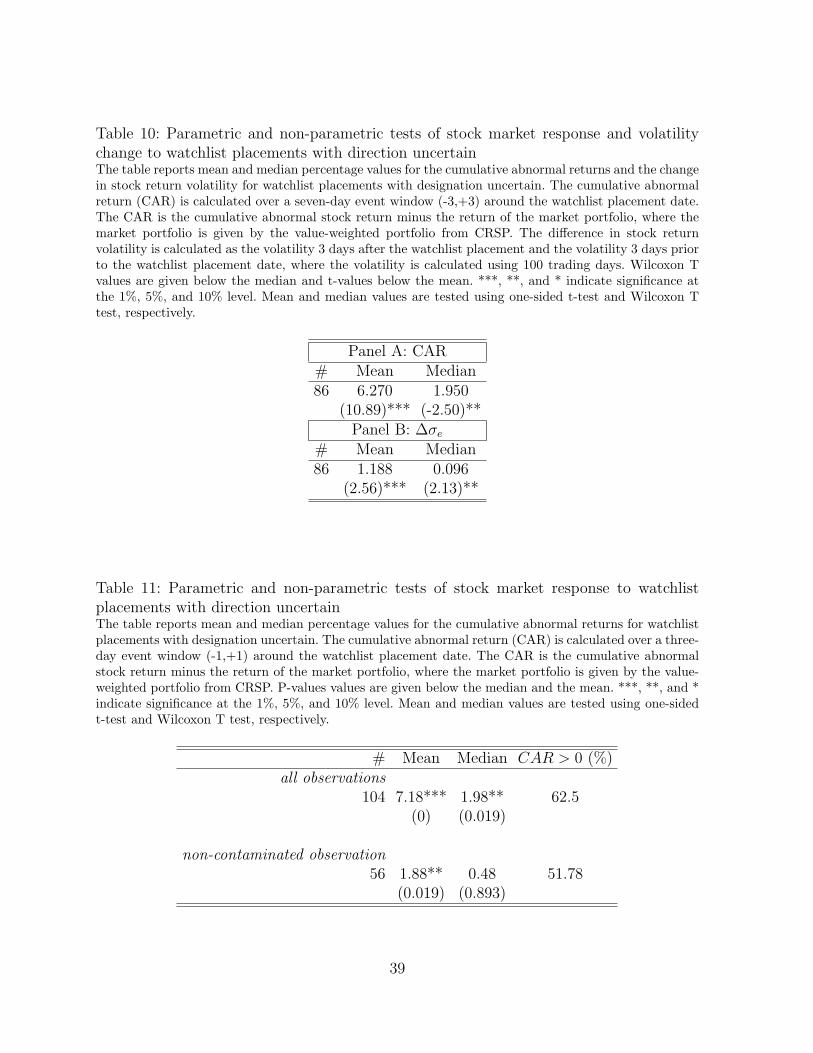
Table 10: Parametric and non-parametric tests of stock market response and volatilitychange to watchlist placements with direction uncertainThe table reports mean and median percentage values for the cumulative abnormal returns and the changein stock return volatility for watchlist placements with designation uncertain. The cumulative abnormalreturn (CAR) is calculated over a seven-day event window (-3,+3) around the watchlist placement date.The CAR is the cumulative abnormal stock return minus the return of the market portfolio, where themarket portfolio is given by the value-weighted portfolio from CRSP. The difference in stock returnvolatility is calculated as the volatility 3 days after the watchlist placement and the volatility 3 days priorto the watchlist placement date, where the volatility is calculated using 100 trading days. Wilcoxon Tvalues are given below the median and t-values below the mean. ***, **, and * indicate significance atthe 1%, 5%, and 10% level. Mean and median values are tested using one-sided t-test and Wilcoxon Ttest, respectively.

Panel A: CAR# Mean Median86 6.270 1.950

(10.89)*** (-2.50)**Panel B: ∆σe

# Mean Median86 1.188 0.096

(2.56)*** (2.13)**

Table 11: Parametric and non-parametric tests of stock market response to watchlistplacements with direction uncertainThe table reports mean and median percentage values for the cumulative abnormal returns for watchlistplacements with designation uncertain. The cumulative abnormal return (CAR) is calculated over a three-day event window (-1,+1) around the watchlist placement date. The CAR is the cumulative abnormalstock return minus the return of the market portfolio, where the market portfolio is given by the value-weighted portfolio from CRSP. P-values values are given below the median and the mean. ***, **, and *indicate significance at the 1%, 5%, and 10% level. Mean and median values are tested using one-sidedt-test and Wilcoxon T test, respectively.

# Mean Median CAR > 0 (%)all observations

104 7.18*** 1.98** 62.5(0) (0.019)

non-contaminated observation56 1.88** 0.48 51.78

(0.019) (0.893)

39

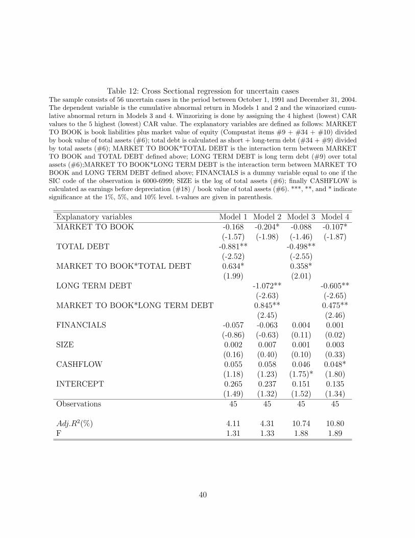
Table 12: Cross Sectional regression for uncertain casesThe sample consists of 56 uncertain cases in the period between October 1, 1991 and December 31, 2004.The dependent variable is the cumulative abnormal return in Models 1 and 2 and the winzorized cumu-lative abnormal return in Models 3 and 4. Winzorizing is done by assigning the 4 highest (lowest) CARvalues to the 5 highest (lowest) CAR value. The explanatory variables are defined as follows: MARKETTO BOOK is book liabilities plus market value of equity (Compustat items #9 + #34 + #10) dividedby book value of total assets (#6); total debt is calculated as short + long-term debt (#34 + #9) dividedby total assets (#6); MARKET TO BOOK*TOTAL DEBT is the interaction term between MARKETTO BOOK and TOTAL DEBT defined above; LONG TERM DEBT is long term debt (#9) over totalassets (#6);MARKET TO BOOK*LONG TERM DEBT is the interaction term between MARKET TOBOOK and LONG TERM DEBT defined above; FINANCIALS is a dummy variable equal to one if theSIC code of the observation is 6000-6999; SIZE is the log of total assets (#6); finally CASHFLOW iscalculated as earnings before depreciation (#18) / book value of total assets (#6). ***, **, and * indicatesignificance at the 1%, 5%, and 10% level. t-values are given in parenthesis.

Explanatory variables Model 1 Model 2 Model 3 Model 4MARKET TO BOOK -0.168 -0.204* -0.088 -0.107*

(-1.57) (-1.98) (-1.46) (-1.87)TOTAL DEBT -0.881** -0.498**

(-2.52) (-2.55)MARKET TO BOOK*TOTAL DEBT 0.634* 0.358*

(1.99) (2.01)LONG TERM DEBT -1.072** -0.605**

(-2.63) (-2.65)MARKET TO BOOK*LONG TERM DEBT 0.845** 0.475**

(2.45) (2.46)FINANCIALS -0.057 -0.063 0.004 0.001

(-0.86) (-0.63) (0.11) (0.02)SIZE 0.002 0.007 0.001 0.003

(0.16) (0.40) (0.10) (0.33)CASHFLOW 0.055 0.058 0.046 0.048*

(1.18) (1.23) (1.75)* (1.80)INTERCEPT 0.265 0.237 0.151 0.135

(1.49) (1.32) (1.52) (1.34)Observations 45 45 45 45

Adj.R2(%) 4.11 4.31 10.74 10.80F 1.31 1.33 1.88 1.89

40