a kernel function approach to exact solutions of calogero ...1001971/fulltext01.pdf · a kernel...
TRANSCRIPT

A kernel function approach to exact solutions ofCalogero-Moser-Sutherland type models
FARROKH ATAI
Scientific thesis for the degree of Doctor of Philosophy (PhD) in the subject areaof Physics.
Stockholm, Sweden 2016
TRITA–FYS 2016:58ISSN 0280–316XISRN KTH/FYS/–16:58–SEISBN 978–91–7729–132–9
KTH Teoretisk fysikAlbaNova universitetscentrumSE-106 91 Stockholm Sweden
Akademisk avhandling som med tillstand av Kungliga Tekniska hogskolan i Stock-holm framlagges till offentlig granskning for avlaggande av Teknologie Doktorsex-amen (TeknD) inom amnesomradet Fysik 27 oktober i Oskar Kleins auditorium(FR4).
c© Farrokh Atai, October 2016
Tryck: Universitetsservice US AB

iii
Abstract
This Doctoral thesis gives an introduction to the concept of kernel func-tions and their significance in the theory of special functions. Of particularinterest is the use of kernel function methods for constructing exact solutionsof Schrodinger type equations, in one spatial dimension, with interactions gov-erned by elliptic functions. The method is applicable to a large class of exactlysolvable systems of Calogero-Moser-Sutherland type, as well as integrable gen-eralizations thereof. It is known that the Schrodinger operators with ellipticpotentials have special limiting cases with exact eigenfunctions given by or-thogonal polynomials. These special cases are discussed in greater detail inorder to explain the kernel function methods with particular focus on the Ja-cobi polynomials and Jack polynomials.
Key words: Kernel functions, Calogero-Moser-Sutherland models, Ruijsenaars-van Diejen models, Elliptic functions, Exact solutions, Source Identities, Chalykh-Feigin-Sergeev-Veselov type deformations, non-stationary Heun equation.
Sammanfattning
Denna doktorsavhandling ger en introduktion till konceptet karnfunktioneroch deras roll i den matematiska teorin for speciella funktioner. Av speci-ellt intresse ar andvandningen av karnfunktionsmetoder i konstruktionen avlosningar till Schrodinger-operatorer i en rumsdiemnsion dar interaktions po-tentialerna ar givna i termer av elliptiska funktioner. Dessa metoder ar aventillampliga pa en storre klass av exakt losbara system av Calogero-Moser-Sutherland-typ, samt integrabla generaliseringar darav. Schrodinger-operatorermed elliptiska potentialer har kanda gransfall dar de exakta losningarna ar or-togonala polynom. Dessa specialfall kommer att behandlas ingaende for att geen mer naturlig forstaelse. Vi kommer i framst att studera Jacobi-polynomenoch Jack-polynomen.
Nyckelord: Karnfunktioner, Calogero-Moser-Sutherland-modeller, Ruijsenaars-van Diejen-modeller Elliptiska funktioner, Exakta losningar, Kallidentiteter,CFVS-deformationer, icke-stationara Heun-ekvationen.

iv
Typeset in LATEX

Preface
This thesis for the degree of Doctor of Philosophy (Ph.D.) in the subject area ofPhysics is to summarize my research at the Theoretical Physics Department of theRoyal Institute of Technology (KTH) in Stockholm, Sweden from 2011 to 2016. Thethesis is divided into two parts: the first provides background and complementaryresults to our research papers. The second consists of four appended scientificpapers.
Overview of the thesis
List of papers included in this thesis
I F. Atai, M. Hallnas, and E. Langmann, Source Identities and Kernel Func-tions for Deformed (Quantum) Ruijsenaars Models, Lett. Math. Phys. (2014)104:811.
II F. Atai and E. Langmann, Deformed Calogero-Sutherland model and fractionalQuantum Hall effect, Preprint: arXiv:1603.06157
III F. Atai and E. Langmann, Series solutions of the non-stationary Heun equation,Preprint: arXiv:1609.02525
IV F. Atai, Integral representation of solution to the non-stationary Lame equation,manuscript
The thesis author’s contribution to the papers
I I performed the calculations and proved the main results of the Paper, basedon an idea by E. Langmann. I also wrote a first draft of the paper and thePaper was finalized in close collaboration.
II The main result of the Paper was proven by me, and I did all the calcula-tions. I wrote a first draft of the paper and the Paper was finalized in closecollaboration.
III The results in Sections 2,3, and 5.1 was obtained independently by both au-thors. I participated in writing the Paper.
v
vi PREFACE
Paper not included in this thesis
1. F. Atai, J. Hoppe, M. Hynek, and E. Langmann, Variational orthogonaliza-tion, Preprint: arXiv:1307.4010
Acknowledgements
Many people have contributed to my development:First and foremost, I would like to give my most heartfelt thanks to my supervi-
sor Professor Edwin Langmann, for his support, patience, and for introducing me tothe exciting fields of special functions and elliptic functions. Words are not enoughto express how grateful I am.
My sincerest gratitude to Martin Hallnas for his insight, comments, and forsharing his vast knowledge of special functions.
I would also like to thank Jack Lidmar and Teresia Mansson for their assistanceduring my Ph.D. studies.
A big thanks to all my current colleagues in the Theoretical Physics department.Thank you; Karl, Daniel, Patrik, Linnea, Anatoly, John, Goran, Mikael, Stella,Mats, and Stefan for many entertaining conversations around the office. Also to myformer colleagues; Johan, Jonas, Hannes, Andreas, Erik, and Richard for creating ahospitable environment. I am also grateful to Olle Edholm for all that he has done,in particular for proofreading this Thesis. I would also like to express my gratitudeto my colleagues at the Mathematics department. I am also pleased to have gottento know Julien and Oskar, whose friendship I cherish. Over the years I have hadthe privilege of sharing office some truly inspiring people. I would like to thankmy former office mates M. Pawellek and J. de Woul. To Per: I will miss our manydiverse discussions, and inspiring arguments, over these last few years.
My heartfelt thanks my family for their love, support, and encouragements:My mother Mehri for her never ending support, Rassul, Shahnaz, Hamid, andAnnalena for their love. And Bahman for his love of, and thoughts on, physicsand mathematics.
To my love: Thank you for your support during this time.
Farrokh Atai(Stockholm, October 27, 2016)

Contents
Preface vAcknowledgements . . . . . . . . . . . . . . . . . . . . . . . . . . . . . . . vi
Contents vii
I Background and complementary results 1
1 Introduction 3
2 Exactly solvable systems of CMS and RvD type 112.1 Classical orthogonal polynomials . . . . . . . . . . . . . . . . . . . . 112.2 Symmetric orthogonal polynomials . . . . . . . . . . . . . . . . . . . 162.3 Exactly solved systems of CMS type . . . . . . . . . . . . . . . . . . 18
3 Systems with elliptic potentials 213.1 One variable cases . . . . . . . . . . . . . . . . . . . . . . . . . . . . 233.2 Many-variable models . . . . . . . . . . . . . . . . . . . . . . . . . . 243.3 Non-stationary elliptic equations . . . . . . . . . . . . . . . . . . . . 25
4 Kernel functions 274.1 Source Identities . . . . . . . . . . . . . . . . . . . . . . . . . . . . . 284.2 Classical orthogonal polynomials . . . . . . . . . . . . . . . . . . . . 284.3 Symmetric polynomials . . . . . . . . . . . . . . . . . . . . . . . . . 334.4 Elliptic potentials . . . . . . . . . . . . . . . . . . . . . . . . . . . . . 35
5 Introduction to scientific papers 395.1 Paper I . . . . . . . . . . . . . . . . . . . . . . . . . . . . . . . . . . 395.2 Paper II . . . . . . . . . . . . . . . . . . . . . . . . . . . . . . . . . . 405.3 Paper III . . . . . . . . . . . . . . . . . . . . . . . . . . . . . . . . . 425.4 Paper IV . . . . . . . . . . . . . . . . . . . . . . . . . . . . . . . . . 42
A Special functions 43A.1 Transcendental functions . . . . . . . . . . . . . . . . . . . . . . . . . 43A.2 Classical orthogonal polynomials . . . . . . . . . . . . . . . . . . . . 43
vii

viii CONTENTS
A.3 Elliptic functions . . . . . . . . . . . . . . . . . . . . . . . . . . . . . 44
B Proof of Theorem 47
Bibliography 49
II Scientific Papers 57

Part I
Background and complementaryresults
1


Chapter 1
Introduction
The theoretical understanding of our physical surroundings is based on suitablemathematical models that effectively describe and predict phenomena observed innature. In exceptional cases, the models can be understood completely by exactanalytical solutions, and the theory of special functions appears naturally in thiscontext. Other instances require approximate or numerical methods, but even theserely on the exceptional cases for points of reference or benchmarks. The theory ofspecial functions plays a significant role in mathematics and physics, both in topicsthat can be found in textbooks and in ongoing research, as we will discuss below.Special functions are useful as many of their properties are known in great de-tail, such as series expansions, integral representations, and generating functions inclosed form that are expressed in terms of more elementary functions. Utilizing spe-cial functions for our models is advantageous since having suitable representationsfor solutions allows us to determine many interesting properties, both qualitativelyand quantitatively.
Early in the studies of physics or mathematics, special functions are introducedwhen solving differential equations arising in important problems such as heat trans-port and wave propagation. In the standard undergraduate courses on electrody-namics, one considers solutions of Laplace and Helmholtz equations in special ge-ometries. These courses provide an introduction to special functions known by thenames Laguerre, Bessel, and Legendre, to name a few. In classical mechanics weget differential equations of varying complexity from Newton’s second law. Thesolution of the Kepler problem played an important role in understanding and ex-plaining celestial mechanics. The problems that have been mentioned also havespecial cases, see e.g. Chapter 3 of [1], where the solutions are given in terms ofelliptic functions1 which play an important role in this work, as is discussed belowand in Chapter 3. Elliptic functions have been studied extensively by Abel, Jacobi,Weierstrass, Hermite, etc., and have also appeared naturally in many different prob-lems in the modern fields of mathematics and physics, some of which are discussed
1Originally, the name was derived from their relation to elliptic integrals, see e.g. Section XXIIof [2].
3

4 CHAPTER 1. INTRODUCTION
below. It suffices, at this point, to describe elliptic functions as natural general-izations of the trigonometric functions, in the same manner as the trigonometricfunctions generalize the rational functions, and to illustrate with an example thatfeatures prominently in our work: The Weierstrass ℘-function, defined as
℘(x) ≡ 1
x2+
∑(n,m)∈Z2\(0,0)
1
(x+ 2ω1n+ 2ω3m)2− 1
(2ω1n+ 2ω3m)2, (1.1)
is an elliptic function with two distinct periods (2ω1, 2ω3), whose ratio is not purelyreal; it generalizes the trigonometric function 1/ sin(πx/2ω1)
2 similar as the lattergeneralizes the rational function 1/x2; see (2.2).
The theory of special functions is essentially equivalent to the theory of quan-tum integrable models, which plays a significant role in the understanding of themicroscopic and quantum regime. In order to discuss these matters we must firstspecify what we mean by a understanding of quantum mechanical models. Thesemodels are defined by a Schrodinger operator, or Hamiltonian, H = T + V thatrepresents the energy, meaning that it has the general form with a kinetic term Tand a potential term V . Solving the quantum mechanical models is equivalent tofinding a complete set of eigenfunctions ψn and corresponding eigenvalues En, i.e.
Hψn = Enψn, (1.2)
and it is then natural to claim that a model is solved if the eigenfunctions ψn, andcorresponding eigenvalues En, have been determined. We often refer to the solvedmodels as exactly solvable. The problem in (1.2) is, in general, a difficult problemand it is at this point that the theory of special functions enters. A paradigm is thehydrogen atom model which is obtained by a canonical quantization of the Keplerproblem and successfully treated by special functions: The model has known eigen-values and (exact) eigenfunctions in terms of (associated) Laguerre and Legendrepolynomials. Another well-known example is the Hermite polynomials which ap-pear as solutions of the simple harmonic oscillator model, defined formally by theSchrodinger operator
− ~2
2m
d2
dx2+mω2
2x2 (x ∈ R), (1.3)
where ~ is Planck’s constant divided by 2π, ω > 0 the coupling strength, and m themass of the particle. Special functions, as those mentioned in the above examples,have provided prototypes for numerous other models; one aim is to develop a similarunderstanding in areas of ongoing research, such as general quantum many-bodyproblems with strongly interacting particles.
In seminal papers [3–5] of Calogero a natural many-variable generalization of(1.3) with strongly interacting, identical particles was solved explicitly. The modelcan be formally defined by a Schrodinger operator of the form
N∑j=1
(− ~2
2m
∂2
∂x2j+mω2
2x2j
)+
∑1≤j<k≤N
κ2
(xk − xj)2(1.4)

5
restricted to the region x ∈ RN : x1 < x2 < . . . < xN, and it is exactly solvable inthe sense that it has known eigenvalues in closed form and exact eigenfunctions interms of a symmetric many-variable generalization of the Hermite polynomials2 forκ2 > −~2/4m. As we will discuss in Section 5.2, the model exhibits exotic particlestatistics when not restricted to the region above [7]. Sutherland [8, 9], inspiredby (1.4), considered a system of strongly interacting, identical particles under theinfluence of a periodic potential, defined by the (formal) Schrodinger operator
N∑j=1
− ~2
2m
∂2
∂x2j+
∑1≤j<k≤N
π2
2mω21
g(g − ~)
4 sin( π2ω1
(xk − xj))2(1.5)
in the region x ∈ [−ω1, ω1]N : −ω1 < x1 < . . . < xN ≤ ω1 (ω1 > 0). The model is
often referred to as the Calogero-Sutherland (CS) model, or the Sutherland model.It also has explicitly known eigenvalues and eigenfunctions given in terms of partic-ular symmetric polynomials, later identified as the Jack polynomials [10] (see alsosection 2.2). The theory of symmetric functions have many different applicationsin both physics and mathematics, such as representation theory [11], algebraic ge-ometry [12], and group theory [13]. (A more extensive discussion can be found ine.g. [14] and references therein.) A comprehensive review of these many applicationsare outside the scope of this thesis but we mention the non-interacting case as anillustrative example: The free fermion3 case of the CS model (i.e. g = ~ in (1.5))has explicitly known eigenfunctions in terms of the Schur polynomials, which yielda useful representation of Slater determinants. We would also like to mention thatthese models have exactly solvable classical limits (i.e. taking ~ → 0 in a suitablemanner) known as the Calogero-Moser models [15].
The examples discussed above, and others which are of great interest in ourwork, fall into a larger family of models that can be defined by formal Schrodingeroperators of the general form
N∑j=1
(− ~2
2m
∂2
∂x2j+ U(xj)
)+
∑1≤j<k≤N
V (xk, xj) (1.6)
with particular external potential U and two-body interaction V ; see Table 2.1 forexamples. The models defined by operators of the form (1.6) are commonly referredto as Calogero-Moser-Sutherland (CMS) type models in the literature. The CMStype models have received great interest as they are soluble4 for a large family ofdifferent potentials U and V in (1.6), which also includes potentials that are givenin terms of elliptic functions, as we will discuss in Chapter 3. A property of manyof the CMS type models, and also the models that are discussed below, is that their
2 The eigenfunctions are also multiplied by a known ground state wave function that includesa Jastrow type [6] term.
3We will not consider spin in this Thesis.4Both quantum integrable and exactly solvable [16] in most cases while only quantum integrable
in some [17].
6 CHAPTER 1. INTRODUCTION
exact eigenfunctions are of the general form ψ(x) = ψ0(x)P (z(x)), with ψ0(x) thegroundstate eigenfunction and P (z) a (symmetric) polynomial that, in many cases,is a natural many-variable generalizations of the classical orthogonal polynomials,such as the Jacobi, Laguerre, Bessel, and Hermite polynomials [18] (see also [16]and references therein). Another remarkable characteristic of the CMS type modelsis the existence of so-called kernel functions which provide a natural tool for con-structing eigenfunctions, allowing us to obtain different representations and proveproperties of these eigenfunctions, and simple determination of the correspondingeigenvalues (see Chapter 4 for definition and simple examples of kernel functions).An advantageous property of the kernel function method to solve CMS type sys-tems is that it naturally extends to the models with elliptic interactions, as we willexplain in Section 4.4. It is known that the models of CMS type can be related toirreducible root systems of classical Lie algebras [17] and Lie super-algebras [19,20],which yields a natural relation between CMS type models and the Laplace oper-ator on symmetric spaces, for special values of the coupling parameters. We willnot discuss these relations in detail but will use the nomenclature of root systems,i.e. AN−1 and BCN , to distinguish different CMS type models, see also Table 2.1.Different interesting generalizations5 of the CMS type models have also been con-structed, and we now turn to certain generalizations that play a more prominentrole in our Papers.
A partially solvable generalization of the CS model (1.5), that is defined by theSchrodinger operator
N∑j=1
− ~2
2mj
∂2
∂x2j+
∑1≤j<k≤N
π2g(mj +mk)(gmjmk − ~)
8ω21 sin( π
2ω1(xj − xk))2
, (1.7)
was constructed by Sen [21] where the particles have different masses. (Note that thedimension of g here is not the same as previously.) The Sen type generalizationsalso exists for the models of CMS type [16]. They are all partially solvable inthe sense that they have an explicitly known exact groundstate, but a completeset of eigenfunctions have not been found. This results hold true for arbitrarymasses and, from a purely mathematical perspective, the particle masses can bearbitrary constants, and we will allow them to also assume negative values. Thenthe eigenvalue equation for the explicitly known groundstate of (1.7) is, in specialcases, equivalent to kernel function identities for pairs of CMS type operators, ordeformations thereof; see below. We refer to the groundstate eigenvalue equationfor the Sen type operators as source identities since it can be used as a source forkernel function identities.
A mathematically natural generalization of the CS models was developed byChalykh, Feigin, Sergeev, and Veselov [19, 20, 22, 23] which incorporates two inde-pendent types of strongly interacting, indistinguishable particles and reduce to thestandard CMS type models when only one particle type remains. This generaliza-tion of the CS model is called the deformed Calogero-Sutherland model, and similar
5In the sense that the CMS models in (1.6) are obtained as special cases.

7
generalizations of other systems is referred to as Chalykh-Feigin-Sergeev-Veselov(CFVS) type deformation. The CFVS type deformation of (1.5) formally definedby the differential operator6
N∑j=1
−~2
2
∂2
∂x2j+
N∑j=1
g~2
∂2
∂x2j+
∑1≤j<k≤N
(πω1)2g(g − ~)
4 sin( π2ω1
(xk − xj))2
+∑
1≤j<k≤N
(πω1)2~2(g − ~)/g
4 sin( π2ω1
(xk − xj))2+
N∑j=1
N∑k=1
(πω1)2~(~− g)
4 sin( π2ω1
(xj − xk))2(1.8)
with N, N ∈ N0 the number of different particles, has exact eigenfunctions givenin terms of the so-called super-Jack polynomials which are of particular interest inPapers II, as we will elaborate on in Section 5.2. The deformed models are in-teresting since they have explicitly known eigenvalues and eigenfunctions in closedform, yet a complete understanding of the deformed models is an area of ongoingresearch. Let us mention one motivating question for our Paper II: The deformedCalogero-Sutherland models does not have a satisfactory interpretation as a stan-dard Quantum Mechanics model since the eigenfunctions are not normalizable (seePaper II for details). It can also be shown that the deformed models reduce to thestandard Calogero-Moser models in the classical limit, i.e. in this limit there existsno dependence on the second type of particles. A pertinent question is then whetherthe deformed Calogero-Sutherland model can describe any physical system. In Pa-per II we propose that the deformed CS model is related to Quantum Field Theory,rather than Quantum Mechanics, and we present an application in the context ofthe Fractional Quantum Hall Effect (see Paper II).
There exists a one-parameter generalization of the CMS type models known asthe relativistic Calogero-Sutherland models. The relativistic model originally ap-peared in the context of the sine-Gordon model [24] and was solved in the classicalsetting by Ruijsenaars and Schneider [25]. The quantum (trigonometric) Ruijse-naars model can formally be defined by the analytic difference operator7 [26]
N∑j=1ε=±
N∏k=1k 6=j
(sin( π2ω1
(xk − xj − iεgβ))
sin( π2ω1
(xk − xj)))12eiε~β∂j
N∏k=1k 6=j
(sin( π2ω1
(xk − xj + iεgβ))
sin( π2ω1
(xk − xj)))12, (1.9)
in the region x ∈ [−ω1, ω1]N : −ω1 < x1 < . . . < xN ≤ ω1 and where β is
the relativistic deformation parameter, proportional to 1/c where c is the speed oflight in vacuum. (We set the particle mass in (1.9) to 1/2 for simplicity.) Theoperator in (1.9) has known eigenvalues and exact eigenfunctions in terms of theMacdonald polynomials [27]. The Ruijsenaars model in (1.9) has a (quantum)integrable generalization when the trigonometric functions are replaced by elliptic
6We set the particle mass to unity for simplicity.7We recall that the operator −i∂j ≡ −i ∂
∂xjis the generator of translations.

8 CHAPTER 1. INTRODUCTION
ones [26]; see Section 3.2. Is it also known that there exists a CFVS type deformationof the operator in (1.9) [28], and we construct a CFVS type deformation of theelliptic Ruijsenaars model in Paper I. The Ruijsenaars models are known to haveintegrable generalizations, in the same sense that (1.6) generalizes (1.5), which areknown as the van Diejen models [29]. To be more specific: The Ruijsenaars modelsare related to the AN−1 root system, and the van Diejen models generalizes to theother relevant root systems. The models of Ruijsenaars-van Diejen (RvD) type arereferred to as relativistic models (see also [30]) due to their reduction to the CMStype models: The analytic difference operator of RvD type reduces to Schrodingeroperator of the form (1.6) in the limit β ↓ 0 after subtracting the relativistic restenergy. To illustrate this, we consider the reduction of (1.5) which is obtained bymultiplying (1.9) with 1/β2, subtracting the constant N/β2, and then taking thelimit β ↓ 0. This yields the Hamiltonian in (1.5).
The CMS and RvD type models have natural generalization where the inter-actions are given in terms of elliptic functions, rather than rational, hyperbolic, ortrigonometric functions, which are amenable to exact treatment. We refer to thesetypes of generalizations as systems with elliptic potentials. As we will elaboratefurther on in Chapter 3, the operators with elliptic potentials can be viewed as themost general in the sense that the other models of CMS, and RvD, type can beobtained by (suitable) limits of the elliptic models. An illustrative example is theelliptic CS model where the 1/ sin2 potential in (1.5) is replaced with the Weierstrass℘-function in (1.1), and (1.5) is obtained in the trigonometric limit, i.e. ω3 → +i∞(see Chapter 3).
A famous example of an operator with an elliptic potential was obtained by Lame[31, 32] when considering the stationary temperature distribution on an ellipsoid.It was implicitly shown by Lame that the Laplace equation can be transformed toan eigenvalue equation for a Schrodinger operator with an elliptic potential, knownas the Lame equation, when transforming to confocal ellipsoidal coordinates. Theaforementioned elliptic CS model can also be viewed as a natural many-variablegeneralization of the Lame equation, in the sense that the two variable case of theelliptic CS model reduces to the Lame equation in the center-of-mass coordinates.We will elaborate more on systems with elliptic potentials in Chapter 3, but wouldlike to conclude this paragraph by mentioning some of the models with ellipticpotential which motivated the work in Papers III and IV. A natural generalization ofthe Lame equation was introduced by Darboux [33], and independently rediscoveredby Treibich and Verdier [34]. This case corresponds to a the Schrodinger operatorwith a so-called Darboux-Treibich-Verdier (DTV) potential (see Eq. (3.11)) canbe reduced to the Heun differential equation. (The relation is explained in moredetails in Section 3.1.) Recent developments have yielded generalizations of theelliptic CMS type models where the period ω3 (see (1.1)) is treated as an additionalvariable. These generalized models are often referred to non-stationary CMS typemodels due to their resemblance to a Schrodinger equation with time dependentpotential. Constructing solutions of the non-stationary Lame (see (3.19)) and thenon-stationary Heun equations is an area of ongoing research [35–45]. In Paper

9
III we construct solutions of the non-stationary Heun equation, defined by theeigenvalue equation for the differential operator
i~2π2mω2
1
κ∂
∂τ− ~2
2m
∂2
∂x2+
1
2m
3∑ν=0
gν(gν − ~)℘(x+ ων) (1.10)
with ω0 ≡ 0, ω1 held constant, ω3 ≡ ω1τ , ω2 ≡ −ω1 − ω3, and (arbitrary) modelparameters (A, gν3ν=0), as well as the non-stationary Lame equation8 by the re-cursive and perturbative algorithm (to all orders) explained in Sections 5.3. As wewill show in Section 3.1, the eigenvalue equation for the operator in (1.10) reducesnaturally to the Heun equation in the κ = 0 case.
Plan of the Thesis
In Chapter 2 we consider the limiting cases of the CMS and RvD type modelsmodels with elliptic potentials. We also recall standard methods for constructingeigenfunctions.
Chapter 3 discusses the CMS and RvD type models with elliptic potentials.In Chapter 4 it is demonstrated how the kernel function methods are used for
constructing solutions of the CMS and RvD type models.Chapter 5 gives a brief introduction to the appended scientific papers.
Notation
We start by setting all fundamental constants to unity throughout this thesis, i.e.c = e = ~ = 1 where c is the speed of light in vacuum, e the elementary charge,and ~ is Planck’s constant divided by 2π. We will (in general) rescale systemswith compact support to be on the interval [−π, π] or tensor products of those; thissimply implies that the constant ω1 (see e.g. (1.1) and (1.5)) is set to π, withoutloss of generality. The general periods are included only when relations betweendifferent models are considered. We denote by N,Z,R, and C the set of positivenatural numbers, all integers, real numbers, and complex numbers, respectively.We denote by N0 the set N
⋃0. We also use the notation x for vectors, i.e. forV an N dimensional vectors space (N ∈ N) then the elements in V are denotedby x where x = (x1, x2, . . . , xN ). We define z(x) = (z(x1), z(x2), . . .) = (z1, z2, . . .)for a vector element x and function z. We will use notation
∑Nj<k as a short-hand
for∑
1≤j<k≤N and so forth. We will use superscripts to distinguish the differentoperators and functions and this notations will carry over different chapters.
8The non-stationary Lame equation is obtained from (1.10) for special values of the parameters,e.g. gν = 0 for ν = 1, 2, 3.


Chapter 2
Exactly solvable systems ofCMS and RvD type
A main goal of our research is to construct solutions of CMS and RvD type modelselliptic potentials (recall that by systems with elliptic potentials we mean modelswhere the interactions are given in terms of elliptic functions; see Chapter 3). Themodels with elliptic potentials have special limiting cases where the interactions aregiven in terms of rational, hyperbolic, or trigonometric functions, and these haveexact eigenfunctions of the general form ψ(x) = ψ0(x)P (z(x)) with correspondingeigenvalues in closed form (as explained below). In Chapter 4 we explain our kernelfunction method for constructing the eigenfunctions using such limiting cases asexamples. In this Chapter we also recall standard methods to construct thesesolutions which then are used as benchmarks to compare with results obtainedusing the kernel function method in Chapter 4.
2.1 Classical orthogonal polynomials
In this Section we consider Schrodinger operators with Poschl-Teller potentials [46]which are obtained from the Lame and Heun equations in the trigonometric limit(see Section 3.1). The systems with Poschl-Teller potentials have exact eigenfunc-tions given in terms of the classical orthogonal trigonometric polynomials, by whichwe mean the Chebyshev, Gegenbauer, and Jacobi polynomials, as we will now dis-cuss.
Gegenbauer polynomials
A simple representative for the CMS type models is defined by a Schrodin-ger operator formally defined as
H(G)(x; g) ≡ − d2
dx2+ g(g − 1)
1
sin(x)2(x ∈ [−π, π]), (2.1)
11

12CHAPTER 2. EXACTLY SOLVABLE SYSTEMS OF CMS AND RVD TYPE
which is the simplest (non-trivial) special case of the Poschl-Teller potential (asexplained below). (The coupling parameter is written as g(g − 1) for reasons thatwill become clear below.) The operator in (2.1) is obtained from the Lame operator(see (3.8)) in the trigonometric limit.
To indicate how such an operator is related to a physical model, we now sketchhow it can appear in Quantum Mechanics. Consider two particles confined on theunit circle (recall that the circumference is then 2π) with an interaction that isproportional to the inverse distance squared. Due to translational invariance, we fixthe first particles position to 0 and the other particles relative position to x. Usingthe method of mirror imaging, we then map the system to the real line and the fullpotential becomes ∑
m∈Z
1
(x+ 2πm)2=
1
4 sin(12x)2. (2.2)
The (formal) operator in (2.1) have explicitly known, exact eigenfunctions1 givenby
ψ(G)n (x; g) ≡ sin(x)gC(g)
n (cos(x)) (n ∈ N0) (2.3)
with C(g)n (z) the Gegenbauer polynomials2, and corresponding eigenvalues (n+ g)2.
We proceed to recall a standard method to derive this results. The operator in (2.1)can be factorized as follows:
H(G)(x; g) = (Q(G))∗Q(G) + g2, Q(G) = − d
dx+ g cot(x), (2.4)
with (Q(G))∗ the formal adjoint of Q(G), and it follows from (2.4) that the eigen-values of H(G)(x; g) are positive and bounded from below by g2. The groundstateeigenfunction can be constructed explicitly by solving the first order differentialequation Q(G)ψ0 = 0, and it is a simple exercise to check that the function
ψ0(x; g) = sin(x)g (2.5)
is the unique solution, up to normalization, of this equation. We now turn ourattention to the other eigenfunctions. We make the ansatz that the eigenfunctionsare of the form ψ(G)(x; g) = ψ
(G)0 (x; g)P (G)(cos(x)), with ψ0(x; g) in (2.5). We
define the differential operator h(G)(z; g) as the similarity transformation of theSchrodinger operator H(G)(x; g) by the groundstate (up to an additive constant)and a change of variables; more specifically, let
h(G)(x; g) ≡ ψ(G)0 (x; g)−1H(G)(x; g)ψ
(G)0 (x; g)− g2
= − d2
dx2− g cot(x)
d
dx
(2.6)
1The index (G) is used in order to distinguish from other cases.2Also known as the ultra-spherical polynomials.

2.1. CLASSICAL ORTHOGONAL POLYNOMIALS 13
(the second line is obtained by straightforward calculation) and make a variablesubstitution to z = cos(x), which transforms (2.6) to the (algebraic) differentialoperator
h(G)(z; g) ≡ (1− z2) d2
dz2− (2g + 1)z
d
dz(2.7)
(it is a simple exercise to check that h(G)(cos(x); g) = −h(G)(x; g)). It follows thatthe functions P (G)(z) are eigenfunctions of the reduced operator3 in (2.7), and thatP (G)(z) are polynomials if the eigenvalues of (2.7) are E (G) = n(n + 2g), withnon-negative integers n. A straightforward inspection shows that the eigenvalueequation for h(G), with eigenvalues n(n+2g), yields the differential equation for the
Gegenbauer polynomials C(g)n (z), i.e.(
(1− z2) d2
dx2− (2g + 1)
d
dx+ n(n+ 2g)
)C(g)n (z) = 0. (2.8)
It follows from standard arguments that the eigenfunctions in (2.3) are orthogonalwith respect to the standard L2([−π, π],dx) inner product, i.e. for n 6= m we have
⟨ψ(G)n
∣∣ψ(G)m
⟩=
∫ π
−πC(g)n (cos(x))C(g)
m (cos(x))(sin(x)2
)gdx = 0 (n 6= m). (2.9)
A simple variable substitution in (2.1) shows that this is equivalent to the orthogo-nality of the Gegenbauer polynomials, with respect to the L2([−1, 1], ω(G)(x; g)dx)
inner product, where ω(G)(x; g) ≡ (1− x2)g−12 , i.e.
(C(g)n , C(g)
m ) ≡∫ 1
−1C(g)n (x)C(g)
m (x)(1− x2)g−12dx = 0 (n 6= m). (2.10)
In Chapter 4 we use kernel functions for constructing eigenfunctions of CMS typemodels, and we will use the Gegenbauer polynomials as an illustrative example.To show that the solutions we obtain are indeed the Gegenbauer polynomials onecan use the inner product in (2.9), but one can also use the following equivalentcondition: Let P (z) be a polynomial of degree n satisfying
P (z) =2nΓ(n+ g)
n!Γ(g)zn +O(zn−1). (2.11)
If P (z) is an eigenfunction of (2.7) then the polynomial is the Gegenbauer polyno-
mial C(g)n , i.e. P (z) = C
(g)n (z), and the eigenvalue is n(n+ 2g).
The eigenfunctions in (2.3) can be used in order to form a complete orthogo-nal basis in the L2([0, π]),dx), or equivalently, a complete orthogonal basis in thesubspace of L2([−π, π]) satisfying ψ(−x) = e−iπgψ(x).
3Here and in the following, we refer to the operators of general form h ≡ ±ψ−10 Hψ0 − E0
as the reduced operators for the Schrodinger operator H with groundstate ψ0 and correspondingeigenvalue E0.
14CHAPTER 2. EXACTLY SOLVABLE SYSTEMS OF CMS AND RVD TYPE
It is clear that the coupling parameter in (2.1) is invariant under g → 1− g and,for this reason, there are two factorizations of the operator H(G) in (2.1): The secondone is like (2.4) with g replaced by 1− g. This naturally suggests that the functionsψ
(G)n (x; 1 − g) are also eigenfunctions of the operator in (2.1). However, it is clear
that these eigenfunctions are only L2 for 1− g > −12 . Thus, for g > 3
2 , there is onlyone unique choice of self-adjoint extension of H(G) in (2.1) allowing for solutionsψ
(G)n in (2.3); for −1
2 < g < 32 there are two different self-adjoint extensions of this
kind corresponding to the same differential operator. As an illustrative example weconsider the case g = 0 (1− g = 1) where (2.1) reduces to the second derivative. Itis known that the Gegenbauer polynomials reduce to the Chebyshev polynomials offirst and second kind, respectively, and using the representation of the Chebyshevswith z = cos(x) yields the eigenfunctions
n
2C(0)n (cos(x)) = cos(nx), sin(x)C
(1)n−1(cos(x)) = sin(nx). (2.12)
We know from e.g. undergraduate courses that (arbitrary) linear combinations of
the functions in (2.12) are eigenfunctions of the operator − d2
dx2, and that we must
specify the self-adjoint extension (by imposing e.g. Dirichlet b.c.) in order to havea self-adjoint operator. We would also like to mention that the non-normalizableeigenfunctions can often be interesting object of study [37,38,47–50].
We can then conclude that the Schrodinger operator in (2.1) is a self-adjointoperator on the domain spanned by the eigenfunctions (2.3) since the eigenfunctionsform a complete orthogonal basis with real eigenvalues, the operator is symmetricwith respect to the L2([−π, π], dx) inner product, and the operator is bounded frombelow by g2.
Jacobi polynomials
There exists a natural one-parameter generalization of the Schrodinger operator in(2.1), formally defined by the Schrodinger operator
H(J)(x; g0, g1) ≡ −d2
dx2+g0(g0 − 1)
4 sin(12x)2+g1(g1 − 1)
4 cos(12x)2, (2.13)
with known eigenfunctions
ψ(J)n (x; g0, g1) = sin(12x)g0 cos(12x)g1P
(g0−12 ,g1−
12 )
n (cos(x)) (2.14)
with P(α,β)n the Jacobi polynomials, and corresponding eigenvalues (n+ 1
2(g0+g1))2.
The trigonometric identity
1
sin(x)2=
1
4 sin(12x)2+
1
4 cos(12x)2
clearly shows that (2.13) reduces to (2.1) in special cases. The potential in (2.13) isthe general form of the Poschl-Teller potential [46]. The operator in (2.13) is also

2.1. CLASSICAL ORTHOGONAL POLYNOMIALS 15
obtained from the Heun equation in (3.11) in the trigonometric limit, as is shown inChapter 3. Our solutions of the non-stationary Heun equation, in Paper III are con-structed such that they reduce to the Jacobi polynomials in the trigonometric limit.As we now discuss, the derivation of (2.14) is very similar to what we explainedabove, and we therefore can be brief.
The operator in (2.13) can be factorized as
H(J)(x; g0, g1) = (Q(J))∗Q(J) + 14(g0 + g1)
2 (2.15)
with
Q(J) ≡ − d
dx+ 1
2g0 cot(12x)− 12g1 tan(12x) (2.16)
and (Q(J))∗ the formal adjoint of Q(J). The groundstate of the operator (2.13) canthen be solved explicitly by Q(J)ψ
(J)0 = 0, and is given by
ψ(J)0 (x; g0, g1) ≡ sin(12x)g0 cos(12x)g1 , (2.17)
with eigenvalue 14(g0 + g1)
2.The reduced Schrodinger operator h(J)(z; g0, g1) of H(J), given by
h(J)(z; g0, g1) ≡ −(1− z2) d2
dz2−(g1 − g0 − (g0 + g1 + 1)z
) ddz, (2.18)
is obtained by a similarity transformation and a change of variable to z = cos(x)(same as for the Gegenbauer polynomials in (2.6)-(2.7)). The eigenvalues n(n +g0 + g1), for non-negative integer n, yield the differential equation for the Jacobipolynomials, i.e.(
(1− z2) d2
dz2+ (g1 − g0 − (g0 + g1 + 1)z)
d
dz− n(n+ g0 + g1)
)y = 0. (2.19)
Thus we can conclude that (2.13) has exact eigenfunctions ψ(J)n (x; g0, g1) (n ∈ N0)
given in (2.14). The eigenfunctions in (2.14) are orthogonal with respect to thestandard L2([−π, π],dx) inner product, and this implies the orthogonality relation
(P (α,β)n , P (α,β)
m )L2(ω(J))
≡∫ 1
−1P (α,β)n (x)P (α,β)
m (x)(1− x)α(1 + x)βdx = 0 (n 6= m), (2.20)
(α = g0 − 12 , β = g1 − 1
2) for the Jacobi polynomials. The Jacobi polynomials areknown to have the expansion
P((g0−1
2 ,g1−12 )
n (z) =Γ(2n+ g0 + g1)
2nn!Γ(n+ g0 + g1)zn +O(zn−1) (2.21)
which can be used to define a unique solution to (2.19). (Recall that Γ(x) is theEuler Gamma function: See also (A.1)).

16CHAPTER 2. EXACTLY SOLVABLE SYSTEMS OF CMS AND RVD TYPE
It is clear by construction that (2.13) reduces to (2.1) for special values of thecoupling g0, g1 and this extends to the eigenfunctions: It follows from (2.11) and(2.21), that the Jacobi polynomials reduce to the Gegenbauer polynomials wheng0 = g1 = g as follows,
P(g−1
2 ,g−12 )
n (z) =Γ (2g) Γ
(n+ g + 1
2
)Γ (n+ 2g) Γ
(g + 1
2
)C(g)n (z). (2.22)
2.2 Symmetric orthogonal polynomials
The models that have been considered in this Chapter have natural many-variablegeneralizations that are also exactly solvable. We now turn to examples that featuresprominently in our Papers, i.e. the CMS type model (see (1.5)) and the (quantum)Ruijsenaars models (see (1.9)). These models describe arbitrary number of indis-tinguishable particles on a circle, and the quantum many-body models we considercan, in many cases, arise from the one-particle models.
The eigenfunctions of the quantum many-variable models are labeled by (pos-itive) integer vectors or partitions, in the same manner that the orthogonal poly-nomials in Section 2.1 were labeled by non-negative integers n. The physical inter-pretation of the partitions are, in this work, the corresponding excitation levels fora system of indistinguishable particles since the quantum numbers can be orderedwithout loss of generality, but there are also different physical interpretations; seePaper II. We proceed to recall some basic definitions of partitions for the conve-nience of the reader and in order for this Thesis to be self-contained. We will followthe notation and convention in [27] and [13].
Partitions
We define a partition λ = (λ1, λ2, . . .) as a sequence of non-negative integers λj indecreasing order, i.e.
λ1 ≥ λ2 ≥ · · ·
where only finitely many of the λj ’s are non-zero. The non-zero λj of a partitionare commonly referred to as parts of the partition λ, and the number of parts is itslength, denoted by `(λ). The weight of this partition, denoted by |λ|, is the sumover its parts, i.e. |λ| ≡∑j λj . It is convenient to not make a distinction betweenpartitions that differ only by a sequence of zeros at the end.
Let λ, µ be two partitions and define the dominance ordering, denoted by ”≤”,by
λ ≤ µ⇔ λ1 + . . .+ λj ≤ µ1 + . . .+ µj , ∀j. (2.23)
The dominance order is only a partial ordering (i.e. there exists partition that arenot comparable, for example, the partitions (4, 1, 0) and (3, 2, 2)).

2.2. SYMMETRIC ORTHOGONAL POLYNOMIALS 17
Jack polynomials
We now can turn to the Calogero-Sutherland model and the Jack polynomials. TheCalogero-Sutherland model [8, 9] is (formally) defined by the Schrodinger operator
H(CS)
N (x; g) ≡N∑j=1
− ∂2
∂x2j+ 2g(g − 1)
N∑j<k
1
4 sin(12(xj − xk))2(2.24)
with xj ∈ [−π, π] for all j = 1, . . . , N . It was shown by Sutherland [8, 9] that acomplete set of eigenfunctions of this operator can be constructed by a methodwhich is remarkably similar to the method we used to construct eigenfunctions ofH(G) in (2.1). The Calogero-Sutherland model has exact eigenfunction ψλ(x; g,N)that are labeled by partitions λ, given by
ψλ(x; g,N) ≡ ψ0(x; g,N)P(1/g)λ (z), zj = eixj , (2.25)
with corresponding eigenvalues∑N
j=1(λj+ 12g(N+1−2j))2, where P
(1/g)λ (z) are the
Jack polynomials. To show this,4 we proceed with the well-known factorization ofthe CS Hamiltonian in (2.24): The Schrodinger operator in (2.24) can be factorizedas [51]
H(CS)
N (x; g) =N∑j=1
(Q(CS)
j )∗Q(CS)
j +1
12g2N(N2 − 1),
Q(CS)
j ≡ − ∂
∂xj+ g
N∑j<k
cot(12(xk − xj)), (2.26)
with (Q(CS)
j )∗ the formal adjoint of Q(CS)
j . The groundstate is obtained by solving
Q(CS)
j ψ0 = 0, for all j = 1, . . . , N . It can be shown by straightforward calculations,and well-known trigonometric identities, that the function
ψ0(x; g,N) ≡N∏j<k
sin(12(xk − xj))g (2.27)
solves these equations and thus is the unique groundstate of the operator (2.24).
The Jack symmetric polynomials P(1/g)λ are uniquely defined by the following
properties5
1. P(1/g)λ = mλ +
∑ν<λ c
(1/g)λ,ν mλ with mλ the monomial symmetric polynomials,
defined asmλ(z1, . . . , zN ) ≡
∑σ
zλσ(1)1 · · · zλσ(N)
N (2.28)
4The discussion is very similar to the discussion of the Gegenbauer polynomials and will there-fore be brief.
5Note that the definition in [27] and [52] are for the Jack functions, which are (in a sense) theJack polynomials in an infinite number of variables.

18CHAPTER 2. EXACTLY SOLVABLE SYSTEMS OF CMS AND RVD TYPE
where the sum is over all distinct permutations of the partition λ, and known
coefficients c(1/g)λ,µ .
2. 〈P (1/g)λ , P
(1/g)ν 〉′1/g = 0, for partitions ν, λ such that ν 6= λ, where the inner
product is defined by
〈Pλ, Pν〉′
1/g ≡1
N !
∮|z|=1
N∏j=1
dzj2πizj
∏j 6=k
(1− zj/zk)g Pλ(z) Pν(z). (2.29)
(This is a non-trivial result proved in e.g. [27] or [52].) One can show that the innerproduct (2.29) is identical with the standard L2 inner product of the eigenfunctionsof the Sutherland Hamiltonian in (2.25), which is of interest in the physics inter-pretation of the CS model as a quantum many-body system (we mention this sincethere are other inner products which are used in the mathematical theory of Jackpolynomials [27, 52]). The Jack polynomials can be constructed by many differentapproaches [8–10, 27, 52], and in Section 4.3 we discuss how the Jack polynomialscan be constructed from the kernel function method.
Macdonald polynomials
Here we would also like to mention another many-variable symmetric polynomial,known as the Macdonald polynomials, which depends on an additional parameter.
The Macdonald polynomials are exact eigenfunctions of the algebraic differenceoperator
MN (z; p, t) ≡N∑j=1
N∏k 6=j
(zj − tzkzj − zk
)Tp(zj) (2.30)
with Tq(zj) defined by Tp(zj)f(z1, z2, . . . zN ) = f(z1, . . . zj−1, pzj , zj+1, . . . , zN ). TheMacdonald operator in (2.30) corresponds to the reduced operator for the relativisticCalogero-Sutherland model, defined by the analytic difference operator in (1.9), withp = e−β, t = e−gβ, and zj = eixj . The relativistic CS model has exact eigenfunctions
ψλ(x; g, β) ≡ ψ0(x; g, β)Pλ(z(x); p, t) (zj = eixj ), (2.31)
with Pλ(z; q, t) the Macdonald polynomials and groundstate ψ0(x; gβ,N) discoveredby Ruijsenaars [53] (it can be found in Paper I, for example).
2.3 Exactly solved systems of CMS type
As we mentioned in the introduction, the CMS type models can be defined byN -variable Schrodinger operator of the general form
N∑j=1
− ∂2
∂x2j+ U(xj) +
N∑j<k
V (xk, xj) (2.32)

2.3. EXACTLY SOLVED SYSTEMS OF CMS TYPE 19
with particular potentials U(x) and V (x, y); see Table 2.1 for examples. (We wishto stress that these lists are not complete.)
The models of CMS type share the common property that they have exactsolutions of the form
ψλ(x) = ψ0(x)Pλ(z(x)), (2.33)
where ψ0 are explicitly known groundstate eigenfunctions, λ a partition of lengthless than or equal to the number of particles N , and Pλ polynomials (see e.g. [16]and references therein). The CMS type operators all have a Quantum Mechanicalinterpretation as Hamiltonians.
There are also CMS type operators where U and V in (2.32) are given in termsof elliptic potentials: see Table 2.2. The elliptic CMS type models are known to beintegrable, i.e. there exists N algebraically independent, and mutually commuting,higher order partial differential operators [17,19,29,56–58]:
N∑j=1
(−i)p∂p
∂xpj+ l.o. (p ∈ N), (2.34)
where l.o. stands for terms that are lower order in derivatives. Constructing theeigenfunctions of the CMS type models with elliptic potentials is an area of ongoingresearch [59–62] as many of the standard methods used for non-elliptic systemscannot be generalized to the elliptic case. In Chapter 4 we illustrate how solutionsof the CMS type models can be constructed using the method of kernel functions,and that the kernel function methods are also applicable for the CMS models withelliptic potentials. The kernel function method was used in [16] in order to constructthe eigenfunctions for the AN−1 potential in Table 2.1 by the recursive algorithmdescribed in Section 4.2. We now turn to discuss the CMS systems with ellipticpotentials and in particular, the Lame and Heun equation.
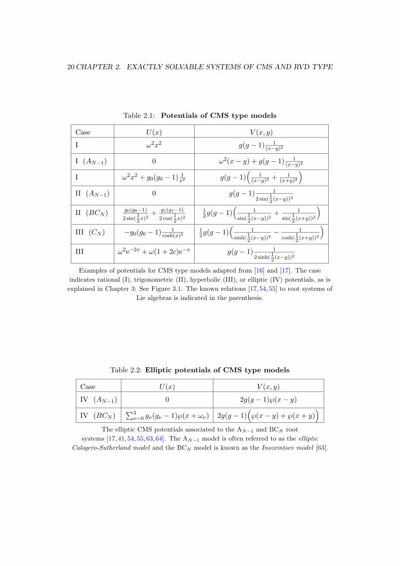
20CHAPTER 2. EXACTLY SOLVABLE SYSTEMS OF CMS AND RVD TYPE
Table 2.1: Potentials of CMS type models
Case U(x) V (x, y)
I ω2x2 g(g − 1) 1(x−y)2
I (AN−1) 0 ω2(x− y) + g(g − 1) 1(x−y)2
I ω2x2 + g0(g0 − 1) 1x2
g(g − 1)(
1(x−y)2 + 1
(x+y)2
)II (AN−1) 0 g(g − 1) 1
2 sin(12 (x−y))
2
II (BCN ) g0(g0−1)2 sin(
12x)
2+ g1(g1−1)
2 cos(12x)
2
12g(g − 1)
(1
sin(12 (x−y))
2+ 1
sin(12 (x+y))
2
)III (CN ) −g0(g0 − 1) 1
cosh(x)212g(g − 1)
(1
sinh(12 (x−y))
2− 1
cosh(12 (x+y))
2
)III ω2e−2x + ω(1 + 2c)e−x g(g − 1) 1
2 sinh(12 (x−y))
2
Examples of potentials for CMS type models adapted from [16] and [17]. The case
indicates rational (I), trigonometric (II), hyperbolic (III), or elliptic (IV) potentials, as is
explained in Chapter 3: See Figure 3.1. The known relations [17,54,55] to root systems of
Lie algebras is indicated in the parenthesis.
Table 2.2: Elliptic potentials of CMS type models
Case U(x) V (x, y)
IV (AN−1) 0 2g(g − 1)℘(x− y)
IV (BCN )∑3
ν=0 gν(gν − 1)℘(x+ ων) 2g(g − 1)(℘(x− y) + ℘(x+ y)
)The elliptic CMS potentials associated to the AN−1 and BCN root
systems [17,41,54,55,63,64]. The AN−1 model is often referred to as the elliptic
Calogero-Sutherland model and the BCN model is known as the Inozemtsev model [63].

Chapter 3
Systems with elliptic potentials
In this chapter we discuss the systems of CMS and RvD type where the interactionsare given in terms of elliptic functions. A famous example of a differential equationwith an elliptic potential was derived by Lame [31, 32] in 1838 when consideringthe stationary temperature distribution on the surface of an ellipsoid. The Lameequation in algebraic form (see below) is known to be a special case of the Heundifferential equation (this relation is discussed when considering the Heun equationin the form of a Schrodinger operator with the Darboux-Treibich-Verdier potential[33, 34,65]). The Lame and Heun equations are discussed in Section 3.1.
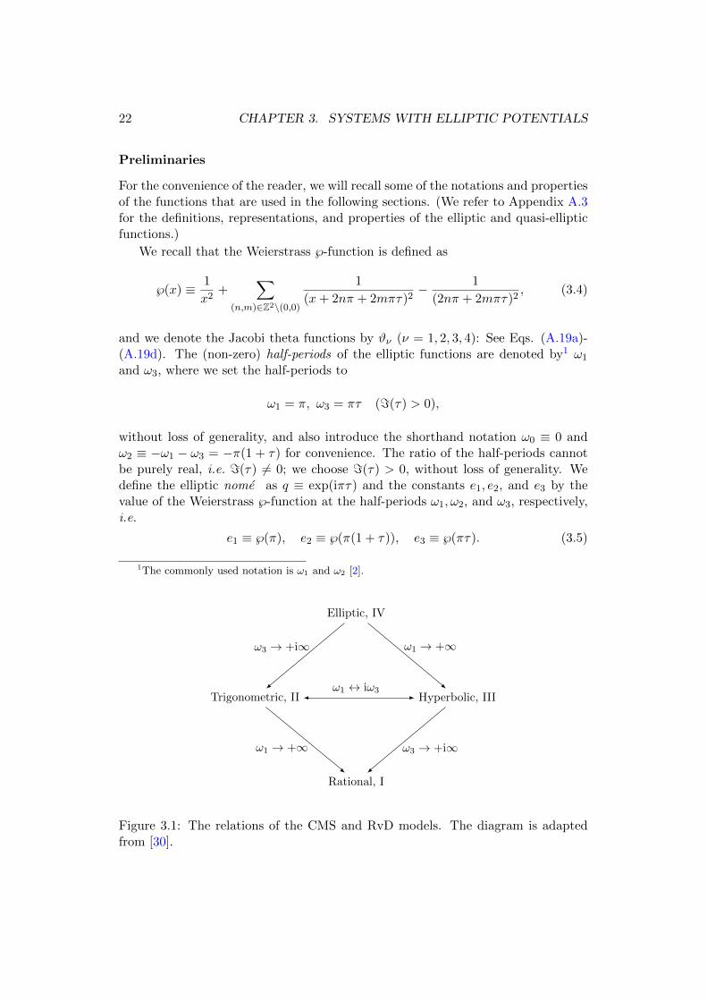
As we have mentioned in Chapter 1, the operators with elliptic potentials canbe considered as the most general of the CMS type Schrodinger operators, in thesense that the other potentials arise from them in suitable limits: See Figure 3.1.These relations can be obtained from the series representation of the Weierstrass℘-function in (1.1), which imply the following results: For x 6= 0(mod(2ω1, 2ω3)),
limω3→+i∞
℘(x|ω1, ω3) =∑n∈Z
1
(x+ 2ω1n)2− 2
∑n∈N
1
(2ω1n)2
=π2
4ω21 sin(12
πω1x)2− π2
12ω21
(=(ω1) = 0); (3.1)
limω1→∞
℘(x|ω1, ia) = − π2
4a2 sinh( π2ax)2+
π2
12a2(ω3 = ia ∈ iR+). (3.2)
It follows from (3.1), and (3.2), that
limω1→∞
limω3→+i∞
℘(x|ω1, ω3) = limω3→+i∞
limω1→∞
℘(x|ω1, ω3) =1
x2. (3.3)
The limits discussed above are representative for all elliptic functions: It wasproven by Weierstrass that any elliptic function can be expressed as rational func-tions of ℘(x), with suitable choices of half periods ω1 and ω3 (see e.g. Chapter XXof [2]); it follows from Weierstrass Theorem that the limiting cases above implysimilar relations for all elliptic functions.
21
22 CHAPTER 3. SYSTEMS WITH ELLIPTIC POTENTIALS
Preliminaries
For the convenience of the reader, we will recall some of the notations and propertiesof the functions that are used in the following sections. (We refer to Appendix A.3for the definitions, representations, and properties of the elliptic and quasi-ellipticfunctions.)
We recall that the Weierstrass ℘-function is defined as
℘(x) ≡ 1
x2+
∑(n,m)∈Z2\(0,0)
1
(x+ 2nπ + 2mπτ)2− 1
(2nπ + 2mπτ)2, (3.4)
and we denote the Jacobi theta functions by ϑν (ν = 1, 2, 3, 4): See Eqs. (A.19a)-(A.19d). The (non-zero) half-periods of the elliptic functions are denoted by1 ω1
and ω3, where we set the half-periods to
ω1 = π, ω3 = πτ (=(τ) > 0),
without loss of generality, and also introduce the shorthand notation ω0 ≡ 0 andω2 ≡ −ω1 − ω3 = −π(1 + τ) for convenience. The ratio of the half-periods cannotbe purely real, i.e. =(τ) 6= 0; we choose =(τ) > 0, without loss of generality. Wedefine the elliptic nome as q ≡ exp(iπτ) and the constants e1, e2, and e3 by thevalue of the Weierstrass ℘-function at the half-periods ω1, ω2, and ω3, respectively,i.e.
e1 ≡ ℘(π), e2 ≡ ℘(π(1 + τ)), e3 ≡ ℘(πτ). (3.5)
1The commonly used notation is ω1 and ω2 [2].
..Elliptic, IV.
Hyperbolic, III
.
Trigonometric, II
.
Rational, I
.
ω3 → +i∞
.
ω1 → +∞
.
ω1 → +∞
.
ω3 → +i∞
.
ω1 ↔ iω3
Figure 3.1: The relations of the CMS and RvD models. The diagram is adaptedfrom [30].

3.1. ONE VARIABLE CASES 23
3.1 One variable cases
Lame equation
The Lame equation can be written as
d2
dx2ψ = (A℘(x) +B)ψ (3.6)
for some constants A and B. We mention this as the Lame equation can be writtenin other forms (see e.g. (3.9)), and that we use the form in (3.6) of the Lame equationas it fits our purpose: We note that Eq. (3.6) reduces to
d2
dx2ψ = (A
1
4 sin(12x)2+ (B − 1
12A))ψ (3.7)
in the trigonometric limit =(τ)→ +∞ (see Eq. (3.1)). (Recall that we set ω1 = πand ω3 = πτ .)
It is convenient to write the Lame equation as an eigenvalue equation for theSchrodinger operator
H(L)(x; g) ≡ − d2
dx2+ g(g − 1)℘(x) (x ∈ [−π, π]), (3.8)
where the constant A is written as g(g− 1) (see also Section 2.1). We note that theelliptic functions are not necessarily real-valued: The Weierstrass ℘-function takesreal values, for x ∈ [−π, π], only when τ is purely imaginary. This clearly showsthat, for arbitrary τ (=(τ) > 0), the operator H(L) in (3.8), and other Schrodingeroperators with elliptic potentials, may not necessarily be symmetric operators.
The eigenfunctions of the operator (3.8), known as the Lame functions, wereoriginally constructed by Lame [31, 32] for special values of the coupling constantand in more generality by Hermite (see e.g. [2]) and Ince [66,67].
The Lame equation in algebraic form, obtained by substituting to the variablez = ℘(x), is given by(− d2
dz2− 1
2(
1
z − e1+
1
z − e2+
1
z − e3)d
dz+
(Az +B)
4(z − e1)(z − e2)(z − e3))ψ = 0. (3.9)
This is a special case of the Heun differential equation which we now proceed todiscuss.
Heun equation
The Heun differential equation is a second order Fuchsian differential equation withfour (regular) singular points (0, 1, t,∞), defined as
d2y
dx2+
(γ
x+
δ
x− 1+
ε
x− t
)dy
dx+
αβx− qHx(x− 1)(x− t)y = 0 (3.10)

24 CHAPTER 3. SYSTEMS WITH ELLIPTIC POTENTIALS
with parameters2 qH, α, β, γ, δ, ε satisfying α+ β + 1 = γ + δ + ε.
We can also write the Heun differential equation as an eigenvalue equation forthe Schrodinger operators with the Darboux-Treibich-Verdier potential, given by
H(DTV)(x; gν3ν=0) ≡ −d2
dx2+
3∑ν=0
gν(gν − 1)℘(x+ ων). (3.11)
where the parameters gν and α, β, γ, δ, ε can have many different relations, e.g.
γ = g0 + 12 , δ = g1 + 1
2 , ε = g2 + 12 , (3.12)
αβ =1
4(g0 + g1 + g2 + g3)(g0 + g1 + g2 − g3 + 1), (3.13)
and the auxiliary parameter qH directly proportional to the eigenvalues of (3.11).It is known that the Heun differential equation (3.10) is the eigenvalue equation forthe reduced Schrodinger operator for H(DTV) in (3.11). (A detailed derivation ofthe relation between (3.10) and (3.11) can be found in [61].) The operator in (3.11)is also the single-particle case of the Inozemtsev Hamiltonian, i.e. the BC1 case inTable 2.2.
3.2 Many-variable models
Elliptic CS model
There exists a natural many-variable generalization of the Lame equation, com-monly referred to as the elliptic Calogero-Sutherland (eCS) model, defined by theSchrodinger operator
H(eCS)
N (x; g) ≡N∑j=1
− ∂2
∂x2j+ 2g(g − 1)
N∑j<k
℘(xj − xk), (3.14)
with xj ∈ [−π, π] for all j = 1, . . . , N . It follows from Eq. (3.1) that the operator(3.14) reduces to the CS operator in (2.24) in the trigonometric limit, i.e.
lim=(τ)→∞
H(eCS)
N = H(CS)
N − g(g − 1)N(N − 1)
24, (3.15)
and the eCS model can be viewed as an elliptic generalization of the CS model.The elliptic Calogero-Sutherland model was originally shown to be quantum inte-grable in [17] and explicit eigenfunctions have been constructed for integer valuesof the coupling g [36, 68]. The eigenfunctions of (3.14) have also been consideredusing standard perturbation theory with expansion in the nome q, using the Jack
2We stress that the auxiliary parameter qH is not the same as the elliptic nome q.

3.3. NON-STATIONARY ELLIPTIC EQUATIONS 25
polynomials [59,69,70]. The eigenfunctions of (3.14) were constructed in [64,71,72]by the perturbative3 algorithm which we discuss in Section 4.4.
The eigenfunctions of the elliptic CS model is assumed to be of similar form as(2.25): The eigenfunctions, constructed in [64,71,72] of the form
ψ(eCS)
λ (x; g,N) ≡N∏j<k
(12q−14ϑ1(
12(xk − xj))
)gPλ(z(x), q2) (zj = eixj , q = eiπτ )
(3.16)with ϑ1 the odd Jacobi theta function and Pλ an elliptic generalization of theJack polynomials, i.e. the functions Pλ reduces to the Jack polynomials in thetrigonometric limit q → 0. The eigenfunctions in (3.16) reduce to the eigenfunctions(2.25) in the trigonometric limit.
Elliptic Ruijsenaars model
We would also like to mention the elliptic (quantum) Ruijsenaars model, defined bythe analytic difference operators
S±(x; gβ) ≡N∑j=1
∏k 6=j
(f∓IV(xk − xj ; g, β)
12
)e∓iβ ∂
∂xj
∏k 6=j
(f±IV(xk − xj ; g, β)
12
)(3.17)
with
f±IV(x; g, β) ≡ ϑ1(12(x± igβ))
ϑ1(12x)
. (3.18)
The operator in (3.17) is known to be quantum integrable [26]. Results in theliterature [73] suggest that this operator has eigenfunctions Pλ(z; q, p, t) which pro-vide and elliptic generalization of the Macdonald polynomials mentioned in Section2.2. The construction of these elliptic Macdonald polynomials is an open area ofresearch, to our knowledge.
3.3 Non-stationary elliptic equations
The work by Olshanetsky and Peremolov [17,54,55] showed that the CMS, and RvD,type models can be related to the irreducible root systems of (classical) Lie algebras,as was discussed in Chapter 1. This gave a natural relation between Schrodingeroperators of CMS type and the Laplace operator in symmetric spaces. It was shownby Etingof, Frenkel and Kirillov [35,74,75] that this approach could be extended toaffine Kac-Moody algebras. Of particular interest is the operator
2i
πκ∂
∂τ− ∂2
∂x2+ g(g − 1)℘(x) (3.19)
3The algorithm is so-called perturbative due to an expansion in a suitable parameter. We stressthat the algorithm is not based on perturbation theory.

26 CHAPTER 3. SYSTEMS WITH ELLIPTIC POTENTIALS
with πτ the half-period of the ℘-function. The eigenvalue equation for the oper-ator in (3.19) is often referred to as the non-stationary Lame equation due to theresemblance with a time-dependent Schrodinger equation
i~∂
∂tψ(x, t) = H(x, t)ψ(x, t). (3.20)
The non-stationary Lame equation is a one-parameter generalization of Lame equa-tion in (3.6), with model parameters (κ, g) that are allowed to take arbitrary values.
The representation theoretic work by Etingof, et. al., was generalized in [45]to the Heun case: The non-stationary Heun equation is defined as the eigenvalueequation for the differential operator
i
πκ∂
∂τ− ∂2
∂x2+
3∑ν=0
gν(gν − 1)℘(x+ ων). (3.21)
(Recall that ω0 ≡ 0, ω1 = π, ω3 = πτ , and ω2 ≡ −ω1 − ω3.) The non-stationaryHeun equation has also appeared when considering different physical models suchas quantum statistical physics for (artificial) spin-ice models [37, 38, 42–44], stringtheory [36, 76], and exact 4-point correlation functions of the quantum Liouvillemodel [39].
In Papers III and IV, the solutions of the non-stationary Heun, and non-station-ary Lame equation, are constructed using the kernel function methods, which weproceed to discuss in the following Chapter.
Chapter 4
Kernel functions
In this Chapter, we introduce and discuss kernel functions with a particular focus ontheir role in the theory of special functions related to CMS, and RvD, type models:We show how the kernel function methods can be used to construct exact eigen-functions of the CMS type models with the different potentials in Tables 2.1 and2.2. We will mainly consider the CMS, and RvD, type models that were discussedin Chapter 3 and the models which are obtained from the elliptic models in thetrigonometric limit; see Chapter 2. The results below illustrates the use of kernelfunctions as a tool for studying special functions.
Preliminaries
We start by establishing some of the basic terminology that is used in this Thesisand our Papers. A function K(x, y) is called a kernel function for a pair of operators(H(x), H(y)) if there exists a constant C such that the functional identity
(H(x)− H(y)− C)K(x, y) = 0 (4.1)
holds. We refer to the functional identity in (4.1) as the kernel function identity.(We write H(x) to indicate that the operator acts on functions depending on thevariable x.) The cases that are of interest in this work will mainly consist of secondorder differential operators or difference operators that have appeared in Chapters2 and 3. An illustrative example is the Schrodinger operator H(G) in (2.1) where itis a simple exercise to check the kernel function identity(
H(G)(x; g)−H(G)(y; g′)) sin(x)g sin(y)g
′
(cos(x)− cos(y))g+g′= 0, (4.2)
holds true (this can be verified by straightforward computations using well-knowntrigonometric identities). Note that the kernel function can always be multiplied byany non-zero constant without changing the kernel function identity in (4.1). It istherefore convenient not to make a distinction between kernel functions that differby a multiplicative (non-zero) constant.
27

28 CHAPTER 4. KERNEL FUNCTIONS
4.1 Source Identities
A systematic approach to finding (explicit) kernel functions is based on the conceptof source identities. The kernel functions, and kernel function identities, that arediscussed in the proceeding chapters are derived from source identities in Refs.[16, 21,41,77,78].
The source identity for the trigonometric Calogero-Sutherland model is due toSen [21], who proved that the exact groundstate eigenfunction of the Schrodingeroperator in (1.7) is
N∏j<k
sin(12(Xj −Xk))gmjmk (4.3)
(To state the result below, we find it convenient to denote the particle number byN , and particle coordinates by Xj for j = 1, . . . ,N .) The identities that are ofparticular interest in our research corresponds to the special cases where the massparameters are restricted to mj ∈ 1,−1, 1/g,−1/g. To illustrate how the sourceidentity in (1.7), and (4.3), can yield other identities, we consider the special casewhere
(Xj ,mj) =
(xj , 1), j = 1, . . . , N
(xj−N ,−1/g), j = N + 1, . . . N + N = N(4.4)
and it follows from a straightforward check that (1.7) reduces to (1.8), and (4.3)becomes the deformed generalization of the CS groundstate. This special case alsoyields the well-known variant of the groundstate eigenvalue equation for the de-formed Calogero-Sutherland model. It is also often more useful to consider thesource identities as the proof for special cases can be more involved than the proofof the source identity [16,41].
4.2 Classical orthogonal polynomials
In order to illustrate the use of the kernel functions, we demonstrate how the well-known eigenfunctions of the Schrodinger operators with the Poschl-Teller potential(see Section 2.1) can be constructed using kernel functions. In these examples, wereproduce results well-known from other methods (see Chapter 2). In the latersections we will proceed to show how the kernel function methods are can be gen-eralized to models with elliptic potentials. (Recall the Schrodinger operator H(G)
in (2.1), ψ(G)n in (2.3), and the Gegenbauer polynomials C
(g)n .)
For g and g′ any complex numbers, the function
K(G)(x, y; g, g′) ≡ sin(x)g sin(y)g′
22g(sin(12(x+ y)) sin(12(x− y)))g+g′(4.5)
satisfy the kernel function identity in (4.7), for the pair of operators (H(G)(x; g), H(G)(y; g′))and C = 0. We now proceed to show how the kernel function in (4.5) can be used to
4.2. CLASSICAL ORTHOGONAL POLYNOMIALS 29
construct integral transforms that map a (generalized) eigenfunction of the operatorH(G)(y; g′) to the eigenfunctions ψ
(G)n (x; g) in (2.3). In particular, we consider the
cases where (g, g′) = (g, 0), (g, g), and (g, g − m), with g arbitrary (m a positiveinteger), as they are illustrative for our discussion in Section 4.4, and Papers IIIand IV.
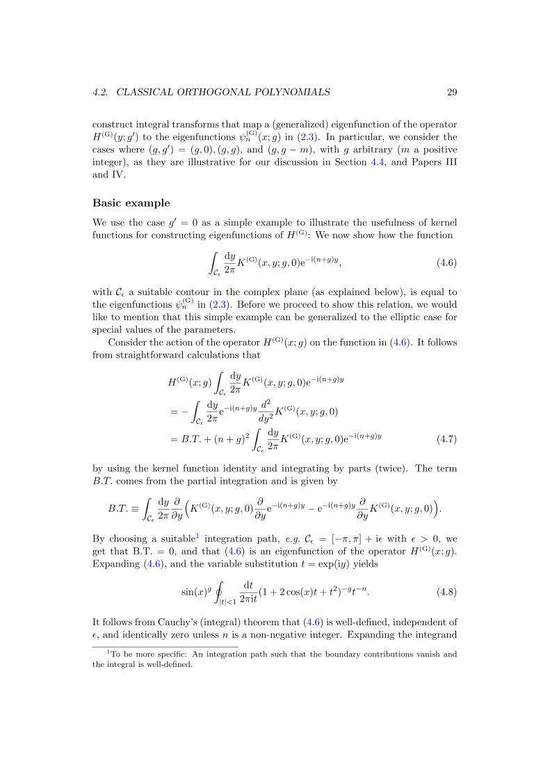
Basic example
We use the case g′ = 0 as a simple example to illustrate the usefulness of kernelfunctions for constructing eigenfunctions of H(G): We now show how the function∫
Cε
dy
2πK(G)(x, y; g, 0)e−i(n+g)y, (4.6)
with Cε a suitable contour in the complex plane (as explained below), is equal tothe eigenfunctions ψ
(G)n in (2.3). Before we proceed to show this relation, we would
like to mention that this simple example can be generalized to the elliptic case forspecial values of the parameters.
Consider the action of the operator H(G)(x; g) on the function in (4.6). It followsfrom straightforward calculations that
H(G)(x; g)
∫Cε
dy
2πK(G)(x, y; g, 0)e−i(n+g)y
= −∫Cε
dy
2πe−i(n+g)y
d2
dy2K(G)(x, y; g, 0)
= B.T.+ (n+ g)2∫Cε
dy
2πK(G)(x, y; g, 0)e−i(n+g)y (4.7)
by using the kernel function identity and integrating by parts (twice). The termB.T. comes from the partial integration and is given by
B.T. ≡∫Cε
dy
2π
∂
∂y
(K(G)(x, y; g, 0)
∂
∂ye−i(n+g)y − e−i(n+g)y
∂
∂yK(G)(x, y; g, 0)
).
By choosing a suitable1 integration path, e.g. Cε = [−π, π] + iε with ε > 0, weget that B.T. = 0, and that (4.6) is an eigenfunction of the operator H(G)(x; g).Expanding (4.6), and the variable substitution t = exp(iy) yields
sin(x)g∮|t|<1
dt
2πit(1 + 2 cos(x)t+ t2)−gt−n. (4.8)
It follows from Cauchy’s (integral) theorem that (4.6) is well-defined, independent ofε, and identically zero unless n is a non-negative integer. Expanding the integrand
1To be more specific: An integration path such that the boundary contributions vanish andthe integral is well-defined.
30 CHAPTER 4. KERNEL FUNCTIONS
as a power series in t shows that the integral represents a polynomial, in cos(x), oforder n; more specifically,∮
|t|<1
dt
2πit(1 + 2 cos(x)t+ t2)−gt−n =
2nΓ(n+ g)
n!Γ(g)cos(x)n + l.d., (4.9)
with ” l.d. ” for the terms of lower degree in cos(x). It follows from the uniquenessof the eigenfunctions (see Chapter 2) that (4.6) is identical with the eigenfunctionψ
(G)n (x; g) in (2.3),i.e.
ψ(G)n (x; g) =
∫Cε
dy
2πK(G)(x, y; g, 0)e−i(n+g)y. (4.10)
Using the kernel function method, we have now re-discovered a well-known expres-sion for the generating functions of the Gegenbauer polynomials (see (A.8)), i.e.
C(g)n (z) =
∮|t|<1
dt
2πit
t−n
(1− 2zt+ t2)g(4.11)
which is equivalent to Eq. (4.10).
Integral equation
To illustrate another use of kernel functions, we consider the case g′ = g. Theintegral transform of the eigenfunction ψ
(G)n (y; g) in (2.3) yield the integral equations
ψ(G)n (x) =
1
λn
∫Cε
dy
2πK(G)(x, y)ψ(G)
n (y), (4.12)
for λn = 22gn!Γ(2g)/Γ(n+ 2g) and, by the uniqueness of the eigenfunctions, yieldsthe relation
C(g)n (z) =
1
λn
∮|t|<1
dt
2πit
(1− t2)2gC(g)n (12(t+ t−1)
(1− 2zt+ t2)2g(4.13)
for the Gegenbauer polynomials. It follows from a straightforward check that thecoefficients of the Gegenbauer polynomials (see (A.7)) satisfy this relations and itis possible to show that this integral equation characterizes the polynomials com-pletely. There also exists similar integral equations for other CMS type systems:We would like to mention the work by Whittaker [79,80], who constructed integralequations for the solutions of the Lame equation,2 and the ellipsoidal harmonicswith the use of kernel functions.
2Whittaker considered the form where the potential is given by sn(x)2, where sn is the ellipticgeneralization of the sine-function [2].
4.2. CLASSICAL ORTHOGONAL POLYNOMIALS 31
Iterative integral representation
The discussion above demonstrated that the construction of eigenfunctions of aCMS type differential operator is equivalent to solving an integral equation usingkernel functions. The kernel functions also allows for explicit integral representationof the eigenfunctions via an iterative scheme, that is easily generalized to the many-variable, and elliptic cases. As an illustrate example, we now discuss the iterativeintegral representation of the Gegenbauer polynomials: Let ψ
(G)n (x; g′) in (2.3) be
an eigenfunction of (2.1) for coupling g′. The integral transform with the kernelfunction K(G)(x, y; g, g′), i.e.∫
Cε
dy
2πK(G)(x, y; g, g′)ψ(G)
n (y; g′), (4.14)
is well-defined iff g− g′ ∈ Z and yields a polynomials in cos(x) of degree n+ g− g′:The function in (4.14) is given by linear combinations of the functions
sin(x)g∮|t|<1
dt
2πit
tν+g−g′(1− t2)2g′
(1− 2 cos(x)t+ t2)g+g′(t = eiy), (4.15)
with ν = −n, . . . n− 1, n. Choosing g′ = g−m, with g−m > 0, yields the recursiverelation
C(g)n−m(cos(x)) =
1
κn,m
∮|t|<1
dt
2πit
tm(1− t2)2(g−m)
(1− 2 cos(x)t+ t2)2g−mC(g−m)n (12(t+ t−1)),
(4.16)with κn,m = (e−iπgΓ(g)Γ(n − 2m − 2g)/n!Γ(2g −m)Γ(g −m)). The constructionof the eigenfunctions then becomes an iteration of the procedure above for theGegenbauer polynomials in the integral. The recursive scheme can be summarizedas follows: The kernel function in (4.14), with g′ = g − m, is the kernel of anintegral transform that maps eigenfunctions of the H(G), with parameter g − m,to eigenfunctions of the H(G) with parameter g. Suppose then that there exists acomplete set of eigenfunctions of the operator H(G) with parameter g = p0, for somep0, then the eigenfunctions of H(G), for parameter g = Nm + p0 with N ∈ N, canbe obtained by the integral transform. The eigenfunctions for g = Nm + p0 willthen be given by an N -fold integral. To illustrate this we consider the case wherem = 1, then the eigenfunctions ψ
(G)n , for coupling g = N , can be expressed as
ψ(G)n (x) =
(N−1∏j=0
∫Cjε
dyj2π
)( 1
κn−j,1K(G)(yj , yj+1;N−j,N−j−1)
)e−i(n+N)yN (4.17)
where Cjε = [−π, π] + ijε with ε > 0, and we identity x = y0, for brevity. Wementioned that the iterative integral method can also be used in the elliptic cases,and in Paper IV we use the kernel functions in order to construct the solutions ofthe non-stationary Lame equation in (3.19); see also Section 4.4. We would like tomention that the integer m = g − g′ in the discussion above is arbitrary for thetrigonometric model. In the elliptic case, it is fixed by the parameter κ (see Section3.3).

32 CHAPTER 4. KERNEL FUNCTIONS
Recursive algorithm
We now turn to the recursive algorithm for constructing eigenfunctions of the CMStype models. In particular, we consider a special case of the results in [16] andPaper III, given by the Schrodinger operator with the general Poschl-Teller potentialin Section 2.1, i.e. H(J) in (2.13). The recursive algorithm can heuristically besummarized as follows: We can construct eigenfunctions of the CMS type modelsin a domain (as explained below) which is not the desired domain from a physics,and often mathematics, point of view. We refer to these formal solutions as thesingular solutions the CMS type Schrodinger operators. The integral transform,with the corresponding kernel function, maps the singular solutions to the standardeigenfunctions, as discussed in Chapter 2, for a suitably chosen integration contour.We proceed to illustrate the recursive algorithm for the Poschl-Teller potential.
Recall the definition of the operator H(J) in (2.13), and the corresponding exacteigenfunctions
ψ(J)n (x) = sin(12x)g0 cos(12x)g1P
(g0−12 ,g1−
12 )
n (cos(x)) (4.18)
with P(α,β)n the Jacobi polynomials. Let λ, g0, g1 be arbitrary complex constants
and define the function K(J) as
K(J)(x, y; g0, g1, λ) ≡ sin(12x)g0 cos(12x)g1 sin(12y)λ−g0 cos(12y)λ−g1
ei12π(λ−g0)2g0+g1(sin(12(x+ y)) sin(12(x− y)))λ
. (4.19)
Then
(H(J)(x; g0, g1)−H(J)(y;λ− g0, λ− g1))K(J)(x, y; g0, g1, λ) = 0. (4.20)
We consider the eigenfunctions of the operator H(J)(y) as linear combinationsof the functions fn = e−i(n+s)y, with n integer and s ∈ R arbitrary (for now), in thedomain =(y) > 0. The operator H(J)(y;λ − g0, λ − g1) acts on the functions fn asfollows
H(J)fn = (n+ s)2fn −∑ν∈N
γνfn−ν , (4.21)
with
γν = 4ν(
(λ− g0)(λ− g0 − 1)− (−1)ν(λ− g1)(λ− g1 − 1)). (4.22)
This follows from the expansion of the operator H(J) as
H(J)(y;λ− g0, λ− g1) = − d2
dy2+∑ν∈N
γνeiνy (=(y) > 0), (4.23)
where we use1
sin(12y)2= −4
∑ν∈N
νe±iνy (=(y) ≷ 0), (4.24)

4.3. SYMMETRIC POLYNOMIALS 33
and shows that the action of the operator has lower triangular structure: H(J)fn isgiven as a linear superposition of functions fm with m ≤ n. The singular eigenfunc-tions of the operator are then given by Fn = fn+
∑m<n αn(m)fm where αn(m) can
be computed exactly (see e.g. [16]). The integral transform with the kernel functionin (4.19) will then transform the singular eigenfunctions to the eigenfunctions ψ
(J)n
in (2.14): It follows from simple trigonometric identities that the function in (4.19)can be expressed as
K(J)(x, y) = ψ(J)0 (x)
e12 i(g0+g1)y(1− eiy)λ−g0(1 + eiy)λ−g1
(1− 2 cos(x)eiy + e2iy)λ. (4.25)
The integral transform is well-defined, for integration contour Cε, if we choose s =12(g0 + g1) (see above), and that the integral transform of the singular solutions aregiven as linear combinations of the functions
ψ(J)0 (x)
∫ π+iε
−π+iε
dy
2π
e−iny(1− eiy)λ−g0(1 + eiy)λ−g1
(1− 2 cos(x)eiy + e2iy)λ(4.26)
with the same coefficients αn(m) as above (up to a normalization constant).Cauchy’s theorem implies that the functions in (4.26) are well-defined, and of theform ψ
(J)0 (x; g0, g1)P (cos(x)) with P a polynomial of degree n ∈ N0. It follows from
the uniqueness of the eigenfunctions that the integral transform of the singularsolutions are the eigenfunction ψ
(J)n in (2.14), i.e.
ψ(J)n (x; g0, g1) = ψ
(J)0 (x)
( π+iε∫−π+iε
dy
2π
e−iny(1− eiy)λ−g0(1 + eiy)λ−g1
(1− 2 cos(x)eiy + e2iy)λ
+∑m<n
αn(m)
π+iε∫−π+iε
dy
2π
e−imy(1− eiy)λ−g0(1 + eiy)λ−g1
(1− 2 cos(x)eiy + e2iy)λ
). (4.27)
We stress that the arguments above are heuristic and that the recursive algo-rithm is mathematically rigorous; see Paper III. We would also like to point out thatthe combination of the recursive algorithm, and the result for the Gegenbauer poly-nomials above (see (A.8)) can yield the explicit coefficient for expansion of Jacobipolynomials in terms of the Gegenbauer polynomials.
4.3 Symmetric polynomials
The kernel function methods can naturally be generalized to many-variable CMStype models and the corresponding symmetric polynomials. To illustrate this, wediscuss how the Jack polynomials, and also Macdonald polynomials, can be con-structed using the kernel functions methods above. (Recall the partitions in Sec-tion 2.2 and the dominance ordering, denoted by ”≤”, in (2.23).) The function

34 CHAPTER 4. KERNEL FUNCTIONS
K(x, y) = K(x, y; g,N,M, p), given by
K(CS)(x, y) =
eip(
N∑j=1
xj−M∑k=1
yk) N∏j<k
(sin(12(xk − xj))g
) M∏j<k
(sin(12(yk − yj))g
)∏Nj=1
M∏k=1
sin(12(xj − yk))g(4.28)
with N,M positive integers, x, y independent complex variables, p an arbitraryconstant, satisfies the kernel function identity(
H(CS)
N (x; g)−HM (CS)(y; g)− CN,M)K(CS)(x, y) = 0 (4.29)
for H(CS)
N in (2.24) and CN,M = (g2/12)(N −M)((N −M)2 − 1) + (N −M)p2.The kernel function in (4.28), for N = M can be used as an integral transform
kernel for the recursive algorithm. Here we take the monomial basis, labeled by apartition n of length N , given by
fn = e−in+1 y1e−in
+2 y2 · · · e−in+
NyN , n+j = nj + sj , (4.30)
with s ∈ RN , in the domain
0 > =(y1) > =(y2) > . . . > =(yN )
The action of the CS Hamiltonian is given by
H(CS)fn =N∑j=1
(n+j )2fn − 4g(g − 1)∑ν∈N
N∑j<k
νfn−ν(ej−ek) (4.31)
with ej is the standard basis in Z, i.e. (ej)l = δj,l, which follows from the many-variable, hypergeometric expansion of the potential, i.e.
H(CS) = −N∑j=1
∂2
∂yj− 4g(g − 1)
N∑j<k
∑ν∈N
νeiν(yj−yk) (4.32)
valid in the domain (see above). It follows by a straightforward check that the oper-ator acts as a lower triangular matrix, i.e. H(CS)fn is given by linear combinationsof fm with m ≤ n w.r.t. the dominance order, and can be diagonalized; see [78,81].The expansion of the kernel function, in this domain, is given by
ei(p+gN)(∑Nj=1 xj−yj )ψ0(x; g,N)
∏Nj=1 ei
12g(N+1−2j)yj∏
j<k(1− ei(yj−yk)g∏Nj,k=1(1− eixj−iyk)g
(4.33)
up to an irrelevant constant, which shows that the integral transform is well-definedif sj = 1
2g(N+1−2j), for j = 1, . . . , N , and that the integral transform will produce
4.4. ELLIPTIC POTENTIALS 35
a symmetric polynomials in eixj (multiplied with the groundstate eigenfunction) forp = −gN . It follows from the uniqueness that the integral transform of the singularsolutions are the eigenfunctions in (2.25).
We would like to mention that the symmetric polynomials can also be con-structed by iterative integrals, as explained in Section 4.2 for the Gegenbauer poly-nomials. This was proven in [82] for the Jack polynomials using the kernel functionin (4.28), with N > M , which was derived from a CFT consideration of the CSmodel that is similar to the work in Paper II. The iterative integral representationfor the Macdonald polynomials is due to Mimachi and Noumi [83]. Recent devel-opments by Hallnas and Ruijsenaars in [84–86] for the hyperbolic AN−1 case (seeTable 2.1) shows that the iterative integral method can also be extended to CMStype models where the eigenfunctions are not given in terms of polynomials.
4.4 Elliptic potentials
The kernel function methods for the CMS models with elliptic potentials are remark-ably similar to the discussion in Section 4.2. A notable difference is in the recursivealgorithm has to be supplemented by an additional series expansion, which we re-fer to as the perturbative algorithm. We consider the Lame equation in order toillustrate the perturbative algorithm. The discussion follows Section 4.2 and will bebrief.
(Recall the Jacobi ϑ-functions (see also Appendix A.3) and the Lame operatorH(L)(x; g) in (3.8).) Let ϑ1 denote the odd Jacobi ϑ-function (see (A.19a)) and g acomplex constant. The function
ϑ1(x)gϑ1(y)g(ϑ1(
12(x+ y))ϑ1(
12(x− y))
)2g (4.34)
satisfies the kernel function identity(H(L)(x; g)−H(L)(y; g)
)K(x, y; g) = 0. (4.35)
with H(L) in (3.8). The singular eigenfunctions are constructed in terms of plane-waves exp(−i(n + s)y), n ∈ Z, s ∈ R as before. It follows from known identitiesof the Weierstrass ℘-function that the operator H(L)(y; g) can be expanded in ahypergeometric series: Let 0 < =(y) < π=(τ), then
H(L)(y; g) = − d2
dy2− 4g(g − 1)
∑ν∈Z
ν1
1− q2ν eiνy − 4g(g − 1)η1π, (4.36)
with η1/π in (A.25). It follows that the H(L) operator does not act as a lowertriangular matrix on the space that is spanned by the plane-waves, and the singulareigenfunctions are then not as straightforward to construct. It was shown in [64]that an additional expansion in the nome q will yield an algorithm which is close

36 CHAPTER 4. KERNEL FUNCTIONS
to the recursive algorithm; see also Paper III. Standard perturbation theory of theelliptic models have usually chosen the nome q, satisfying |q| < 1, as a natural smallparameter in the perturbative expansion [59,61].
It is known that the kernel functions for CMS type models with elliptic po-tentials, can only satisfy kernel function identities, such as (4.35) under certainrestrictions on the parameters or the particle numbers. These restrictions are oftenreferred to as balancing conditions. One can show that the kernel functions satisfygeneralized kernel function identities if the balancing condition is removed: Thefunction
K(L)(x, y, τ ; g, g′) ≡ ϑ′1(0)g+g′ϑ1(x)gϑ1(y)g
′
(ϑ1(12(x− y))ϑ1(
12(x+ y)))g+g′
(4.37)
with g, g′ arbitrary complex constants, ϑ1(x) = ϑ1(x|πτ), ϑ1(y) = ϑ1(y|πτ), satisfiesthe generalized kernel function identity(2i
π(g − g′) ∂
∂τ+H(L)(x; τ, g)−H(y; τ, g′)− c1
)K(L)(x, y, τ ; g, g′) = 0, (4.38)
for c1 = 2(g − g′)(1 − g − g′)η1/π [41]. It follows from that the integral transformmaps solutions of the non-stationary Lame equation with coupling κ = g − g′, g′ tosolutions with coupling κ = g − g′, g; as discussed in Paper IV.
We now turn to the Heun equation and some new results. Define gµν ( µ, ν =0, . . . , 3) as
gµ0gµ1gµ2gµ3
=
δµ,0 δµ,1 δµ,2 δµ,3δµ,1 δµ,0 δµ,3 δµ,2δµ,2 δµ,3 δµ,0 δµ,1δµ,3 δµ,2 δµ,1 δµ,0
g0g1g2g3
(4.39)
with gν the model parameters of the Heun equation (see (3.11)). (The Jacobi ϑ-functions given in (A.19a)-(A.19b), and the operator H(DTV)(x; gµν 3ν=0) in (3.11).)
Theorem 4.4.1. Let µ ∈ 0, 1, 2, 3 be fixed, gµν as in (4.39) and gµν = λ − gµν ,with λ = 1
2
∑3ν=0(gν − 1
4κ). The function
K(DTV)µ (x, y, τ ; g, g) ≡
3∏ν=0
(ϑν+1(12x)gνϑν+1(
12y)g
µν )(
ϑµ+1(12(x− y))ϑµ+1(
12(x+ y))
)λ (4.40)
satisfies the generalized kernel function identity( i
πκ∂
∂τ+H(DTV)(x; gν3ν=0)−H(DTV)(y; gµν 3ν=0)− C1,1
)K(DTV)µ (x, y, τ) = 0
(4.41)with constant C1,1 = 2κ(1− λ)(η1/π) and η1 in (A.25).
(The µ = 0 case was proven in [41]. The cases where µ = 1, 2, 3 are new, to ourknowledge, and the proof is given in Section B.)
The result in Theorem 4.4.1 for the non-stationary Heun equation yields thefollowing results as special cases.

4.4. ELLIPTIC POTENTIALS 37
Corollary 4.4.2. The function in (4.40) for κ = 0 (i.e. λ = 12
∑3ν=0 gν) is a ker-
nel function for a pair of Schrodinger operators with the Darboux-Treibich-Verdierpotential, i.e.(
H(DTV)(x; gν)−H(DTV)(y; gµν ))K(DTV)µ (x, y) = 0, (µ ∈ 0, 1, 2, 3) (4.42)
for gν3ν=0 complex constants, gµν = (12∑3
ν=0 gν)− gµν , and H(DTV) in (3.11).
The µ = 0 case was obtained in [41] and the µ = 3 case was obtained in [87] asthe limit of a kernel function for the elliptic van Diejen model. (The µ = 1, andµ = 2, cases are new, to our knowledge, but follows from the results in [41] and [87]by a simple shift.)
Corollary 4.4.3. For gν = g for all ν = 0, . . . 3 the kernel function in (4.40)reduces to
K(L)µ (x, y, τ ; g, κ) ≡ ϑ1(0)2g−κ
ϑ1(x)gϑ1(y)g−κ(ϑµ+1(
12(x+ y))ϑµ+1(
12(x− y))
)2g−κ (4.43)
and satisfies the generalized kernel function identity(2i
πκ∂
∂τ+H(L)(x; g)−H(L)(y; g − κ)− c(L)
)K(L)µ (x, y, τ) = 0 (4.44)
with constant c(L) = 4κ(1 + κ− 2g)(η1/π).
In paper III, we use the kernel function in (4.42), with µ = 1, for the perturbativealgorithm for the non-stationary Heun equation, and the kernel function in (4.43)is used for iterative integral representations of the non-stationary Lame equation inPaper IV.


Chapter 5
Introduction to scientific papers
The purpose of this chapter is to introduce the results that are obtained in the fourscientific papers appended to this Thesis.
5.1 Paper I
In Paper I we consider the Ruijsenaars models (i.e. AN−1 relativistic Calogero-Sutherland models) with different types of interaction given in terms of rational,hyperbolic, trigonometric, and elliptic functions. The Ruijsenaars models are ex-pressed in terms of the function s(x), defined as
s(x) ≡
x (Rational case (I))
2 sin(12x) (Trigonometric case (II))
(a/π) sinh(πx/a) (Hyperbolic case (III))
ϑ1(12x|i12a) (Elliptic case (IV))
(5.1)
with ϑ1 the Jacobi theta function in (A.19a). This is notation is convenient as itallows for a unified approach (as shown in Paper I).
We construct a restricted Sen type generalization (source identity) of the Rui-jsenaars model where the mass parameters only take values in the set
Λ = m0,−m0,−1/gm0, 1/gm0
with m0 some fixed non-zero constant (see also Section 4.1. The Sen type general-ization is defined by the (formal) analytic difference operators
S±(x;m, g, β) ≡N∑j=1
s(igmjβ)
igβs′(0)A∓j (x;m, g, β)e
∓i βmj
∂∂xjA±j (x;m, g, β) (5.2)
with particular interaction A±j that can be found in Paper I. In order to illustratethe unified approach, we consider the special case where all the mass parametersare set to unity and the interactions reduce to the interaction in (3.17)-(3.18).
39

40 CHAPTER 5. INTRODUCTION TO SCIENTIFIC PAPERS
The operator in (5.2) is interpreted as a relativistic generalization of the SenHamiltonian in (1.7) as it is obtained by
limβ→0
(β−2
(S+ + S−
)−
N∑j=1
mjβ−2). (5.3)
For the elliptic case, we can only construct an exact groundstate of (5.2) underthe restriction of the balancing condition
∑Nj=1mj = 0 (see Section 4.4).
The source identity was then used in order to give a unified derivation of pre-viously well-known identities in [26, 28, 88] and the CFVS type deformation of thetrigonometric Ruijsenaars model [28]; see Sections 3 and 4 of Paper I . The newresults in Paper I is a CFVS type deformations of the Ruijsenaars model when theinteractions are given by elliptic functions (Case IV above). The integrability ofthe elliptic CFSV type deformation of (1.9) is conjectured by the existence of anexplicit kernel function.
5.2 Paper II
It is known that the CS model has a collective field theory representation [82,89–91]that is related to exotic particles known as anyons [92, 93] (explained below) andthe Fractional Quantum Hall Effect (FQHE). The Calogero and CS models havenaturally appeared in the theory of the FQHE [7, 48, 89, 94, 96, 97] and anyons.Anyons are quasiparticles that exhibit exotic particle statistics, i.e.
φ(x)φ(y) = e±iαπφ(y)φ(x) for x ≷ y and α ∈ R (5.4)
which are not restricted to only fermions (α = 1) or bosons (α = 0), and they canappear in lower dimensional systems. The FQHE was exceptional (when discovered)due to the high precision of measurement results which intuitively suggest a theoret-ical explanation by an exactly solvable systems. The results in Paper II show thatthe previously known relation between the FQHE and the CS model can naturallybe extended to the deformed model. We would like to mention that the collectivefield theory can also be extended to include the elliptic Calogero-Sutherland modelin (3.14) [71,72].
The collective field theory (CFT) approach is also closely related to the approachin [98] utilizing symmetric functions (SF). It follows from the fact that the CFT andSF approaches are different representations of the (extended) Heisenberg algebra(see e.g. [99]). We prove that the collective field theory construction of the CS model,defined by a operator, which we denote by Hν,3, and which is explicitly known (seePaper II), is in fact the collective field theory description of the deformed Calogero-Sutherland (dCS) model, defined by the differential operator in (1.8): Define thevertex operator φν(x) in terms of free bosons that satisfy a U(1) affine Kac-Moody

5.2. PAPER II 41
algebra, i.e. ρn (n ∈ Z) and R satisfying
[ρn, ρm] = nδn+m,0, ρ†n = ρ−n, (n,m ∈ Z) (5.5)
[ρn, R] = δn,0R, R† = R−1. (5.6)
We prove that the differential operator defining the deformed CS model in (1.8)(see also Eq. (5) in Paper II), which we denote by HN,N , acting on a product of
vertex operators is the action of the operator Hν,3 on the same product of vertexoperators: To be precise, for g = ν2 the following holds
Hν,3φν(x1) . . . φν(xN )φ− 1ν(x1) · · ·φ− 1
ν(xN )|0〉
=(HN,N (x, x) + c)φν(x1) . . . φν(xN )φ− 1ν(x1) · · ·φ− 1
ν(xN )|0〉, (5.7)
with c constant and |0〉 the vacuum state satisfying ρn|0〉 = 0, n ≥ 0, and 〈0|RQ|0〉 =δQ,0. We would like to mention that these results were anticipated in the physicsliterature [94].
In Paper II we utilize the relation to the deformed Calogero-Sutherland model,using known mathematical results about the super-Jack polynomials, in order toconstruct a set of orthogonal eigenstates for the collective field theory: The dCSmodel is known [23] to have exact eigenfunctions
ψλ(x, x; g) = ψ0(x, x; g)SPλ(z, z; g), zj = eixj , zj = eixj , (5.8)
labeled by partitions in the so-called fat (N, N)-hook, i.e. λN+1 ≤ N and `(λ)arbitrary. (We wish to stress that the function ψ0 is not a groundstate eigenfunctionin the quantum mechanical meaning. We abuse physics terminology and often referto ψ0 as the deformed groundstate.)
We construct the orthogonal eigenstates as
N∏j=1
∫Cε
dxj2π
N∏k=1
∫Cε′
dxk2π
ψλ(−x,−x; ν2)φν(x1) . . . φν(xN )φ− 1ν(x1) · · ·φ− 1
ν(xN )|0〉,
(5.9)which we refer to as super-Jack states. The orthogonality of the super-Jack statesfollows from known identities [19,23,95], such as the integral relations of the super-Jack polynomials
N∏j=1
∫Cε
dxj2π
N∏k=1
∫Cε′
dxk2π
ψ0(x, x)2SPλ(z, z)SPµ(z−1, z−1) = 0 (λ 6= µ), (5.10)
and that the differential operator HN,N in (1.8) is symmetric if we were to consider(5.10) as an inner product. (The integral is well-defined for ε 6= ε′ and we use theshorthand z−1 = (z−11 , . . .) etc.)
42 CHAPTER 5. INTRODUCTION TO SCIENTIFIC PAPERS
5.3 Paper III
Paper III considers the non-stationary Heun equation in (1.10) for arbitrary modelparameters (κ, gν3ν=0). We show that constructing eigenfunctions of the operatorin (1.10) is equivalent to finding solutions of a differential-difference equation: Thekernel functions are used in order to construct a particular set of basis functionsFm(x)m∈Z (as described in Section 4.2). The solutions of the non-stationary Heunequation is constructed by linear combinations of the basis functions Fm, i.e.
ψn(x) =∑m∈Z
αn(m)Fm(x) (5.11)
where the coefficients αn(m) satisfy the differential-difference equation in Section3 of Paper III. In Section 5 of Paper III we present two algorithms for computingthe coefficients αn(m), expanded in a power series in the nome q. We note thatthese series solutions of the non-stationary Heun equation is especially suited whenthe model parameters take complex values. However, there are difficulties with theperturbative algorithm when the model parameters take integer values.
A remarkable feature of the kernel function method is that the methods de-veloped for the elliptic Calogero-Sutherland model in [64] generalizes to the non-stationary Heun equation, with model details only changing building blocks of thesolutions.
5.4 Paper IV
In Paper IV we present a recursive scheme for constructing solutions of the non-stationary Lame equation, which yields iterative integral representations of thesesolutions (as explained in Section 4.2). The integral step for the iterative integralrepresentation of the Gegenbauer polynomials are determined by the model param-eter κ, i.e. κ = g − g′, in generalization of (4.15). This shows that the iterativeintegral representations are especially suited for integer values of the model pa-rameters and serves as a complementary approach to the perturbative algorithm inPaper III.
A remarkable property is the existence of Hilbert-Schmidt class integral trans-form operators that allow us to construct iterative integral representations of thesolutions for arbitrary values of the model parameters. (Recall that in Section 4.2there was a requirement g − g′ ∈ Z.)
The recursive procedure in Paper IV is then used to construct explicit integralrepresentation for special cases of the model parameters.

Appendix A
Special functions
We collect standard definitions and results about special functions: a standardreference is [2], for example.
A.1 Transcendental functions
The Euler Γ function can expressed as
Γ(x) =1
ze−γz
∞∏l=1
(1 +
z
n
)−1ez/n, (A.1)
with γ = limm→∞∑m
l=1(1/n) − ln(m) ≈ 0.5772157 the Euler constant. The EulerΓ(x) function has simple poles at x ∈ −N0 which can be seen from the differenceequation
Γ(x+ 1) = xΓ(x) (A.2)
The (raising) Pochhammer symbol (x)n is defined as
(x)n = x(x+ 1) · · · (x+ n− 1) (n ∈ N0), (A.3)
for non-negative integers n. The Pochhammer symbol can be represented as
(x)n =Γ(x+ n)
Γ(x)(A.4)
for all x, n ∈ C.
A.2 Classical orthogonal polynomials
The Gegenbauer polynomials C(g)n are the unique solutions of the differential equa-
tion((1− x2) d
2
dx2− (2g + 1)x
d
dx+ n(n+ 2g)
)C(g)n (x) = 0 (g > 0, n ∈ N0), (A.5)
43

44 APPENDIX A. SPECIAL FUNCTIONS
with expansion
C(g)n (x) =
2n(g)nn!
xn + l.o. (A.6)
where (g)n is the raising Pochhammer symbol; see (A.3) and (A.4).The Gegenbauer polynomials have the series representation
C(g)n (x) =
(2g)nn!
n∑ν=0
(−n)ν(n+ 2g)ν
(g + 12)ν
(1− x2
)ν(A.7)
The Gegenbauer polynomials have a generating function given by
1
(1− 2xξ + ξ2)g=∑n∈N0
C(g)n (x)ξn (A.8)
where the series is absolutely convergent for x in the interior of an ellipse in thecomplex plain with focal points ±1 and semi-major axis 1
2(ξ+ ξ−1). For x ∈ [−1, 1]the series is absolutely and uniformly convergent for |ξ| < 1.
The Jacobi polynomials P(α,β)n (x) are the unique solutions of the differential
equation((1−x2) d
2
dx2+(β−α−(α+β+2))x
d
dx+n(n+α+β+1)
)P (α,β)n (x) = 0 (n ∈ N0),
(A.9)with expansion
P (α,β)n (x) =
(n+ α+ β + 1)n2nn!
xn + l.d. (A.10)
The Jacobi polynomials have the series representation
P (α,β)n (x) =
n∑l=0
(n+ α+ β + 1)l(α+ l + 1)n−ll!(n− l)!
(x− 1
2
)l(A.11)
A.3 Elliptic functions
In this appendix we will introduce the elliptic (and quasi-elliptic) functions that weuse in this work. We mainly follow the convention in [2].
Definition A.3.1. Let ω1 and ω3 be any two non-zero numbers such that ω3/ω1 isnot purely real. A double-periodic function is any function satisfying
f(z + 2ω1) = f(z), f(z + 2ω3) = f(z)
for all z in C and an elliptic function is any double-periodic function that is mero-morphic in the finite part of the complex plane.
We refer to the constants ω1, ω3 as the half-periods of the elliptic functions anddefine ω2 ≡ −ω1 − ω3.
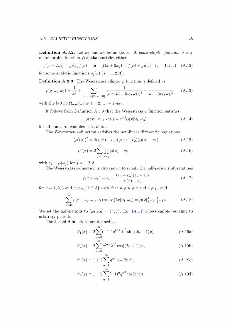
A.3. ELLIPTIC FUNCTIONS 45
Definition A.3.2. Let ω1 and ω3 be as above. A quasi-elliptic function is anymeromorphic function f(x) that satisfies either
f(x+ 2ωj) = gj(x)f(x) or f(x+ 2ωj) = f(x) + gj(x) (j = 1, 2, 3) (A.12)
for some analytic functions gj(x) (j = 1, 2, 3).
Definition A.3.3. The Weierstrass elliptic ℘ function is defined as
℘(x|ω1, ω3) =1
x2+
∑(n,m)∈Z2\(0,0)
1
(x+ Ωn,m(ω1, ω3))2− 1
Ωn,m(ω1, ω3)2(A.13)
with the lattice Ωn,m(ω1, ω3) = 2nω1 + 2mω3.
It follows from Definition A.3.3 that the Weierstrass ℘ function satisfies
℘(cx | cω1, cω3) = c−2℘(x|ω1, ω3) (A.14)
for all non-zero, complex constants c.The Weierstrass ℘-function satisfies the non-linear differential equations
(℘′(x))2 = 4(℘(x)− e1)(℘(x)− e2)(℘(x)− e3) (A.15)
℘′′(x) = 23∑j=1
∏k 6=j
℘(x)− ek (A.16)
with ej ≡ ℘(ωj) for j = 1, 2, 3.The Weierstrass ℘-function is also known to satisfy the half-period shift relations
℘(x+ ων) = eν +(eν − eµ)(eν − eε)
℘(x)− eν(A.17)
for ν = 1, 2, 3 and µ, ε ∈ 1, 2, 3 such that µ 6= ν 6= ε and ε 6= µ, and
3∑ν=0
℘(x+ ων |ω1, ω3) = 4℘(2x|ω1, ω3) = ℘(x|12ω1,12ω3). (A.18)
We set the half-periods to (ω1, ω3) = (π, τ). Eq. (A.14) allows simple rescaling toarbitrary periods.
The Jacobi ϑ-functions are defined as
ϑ1(x) ≡ 2∞∑n=0
(−1)nq(n+12)
2
sin((2n+ 1)x), (A.19a)
ϑ2(x) ≡ 2
∞∑n=0
q(n+12)
2
cos((2n+ 1)x), (A.19b)
ϑ3(x) ≡ 1 + 2∞∑n=1
qn2
cos(2nx), (A.19c)
ϑ4(x) ≡ 1− 2∞∑n=1
(−1)nqn2
cos(2nx). (A.19d)

46 APPENDIX A. SPECIAL FUNCTIONS
where ϑν(x) = ϑ(x, q) = ϑν(x|πτ) with q = exp(iπτ). It follows from the Jacobitriple product identity that the Jacobi ϑ-functions can be expressed as
ϑ1(x, q) = 2q14 sin(x)
∞∏l=1
(1− q2l)(1− 2q2l cos(2x) + q4l) (A.20a)
ϑ2(x, q) = 2q14 cos(x)
∞∏l=1
(1− q2l)(1 + 2q2l cos(2x) + q4l) (A.20b)
ϑ3(x, q) =
∞∏l=1
(1− q2l)(1 + 2q2l−1 cos(2x) + q4l−2) (A.20c)
ϑ4(x, q) =
∞∏l=1
(1− q2l)(1− 2q2l−1 cos(2x) + q4l−2) (A.20d)
It follows from the definition that the Jacobi ϑ-functions satisfy the shift relations
ϑ1(x± π2 τ) = ±ie∓ixq−
14ϑ4(x), ϑ2(x± π
2 τ) = e∓ixq−14ϑ3(x)
ϑ3(x± π2 τ) = e∓ixq−
14ϑ2(x), ϑ4(x± π
2 τ) = ±ie∓ixq−14ϑ1(x). (A.21)
The function ϑν(x) has simple zeros at the points x = ων/2(mod(ω1, ω3)) withω1 = π, ω3 = πτ .
The Jacobi ϑν functions all satisfy the differential equation
(πi
4
∂2
∂x2+
∂
∂τ)ϑν(x|πτ) = 0 (ν = 1, 2, 3, 4). (A.22)
The Jacobi functions satisfy the double angle formula
ϑ1(2x) =2
ϑ′1(x)ϑ1(x)ϑ2(x)ϑ3(x)ϑ4(x) (A.23)
The Weierstrass ℘-function can be expressed in terms of the Jacobi functions as
℘(x+ ων) =1
4
((ϑ′ν+1(12x)
ϑν+1(12x)
)2− ϑ′′ν+1(
12x)
ϑν+1(12x)
)− η1π
(A.24)
withη1π
= − 1
12
ϑ′′′1 (0)
ϑ′1(0)=
1
12− 2
∞∑l=1
q2l
(1− q2l)2 (A.25)
Appendix B
Proof of Theorem
In this Section we present the proof of Theorem 4.4.1. We recall that Theorem 4.4.1concerned the generalized kernel function identity( i
πκ∂
∂τ+H(DTV)(x; gν3ν=0)−H(DTV)(y; gµν 3ν=0)− C1,1
)K(DTV)µ (x, y, τ) = 0
(B.1)for K
(DTV)µ (x, y, τ) in (4.40). As we already mentioned, the µ = 0 case was proven
in [41] (see also Paper IV). The µ = 1 case follows from their results by x→ x+ πwhere
3∑ν=0
gν(gν − 1)℘(y + π + ων) = g0(g0 − 1)℘(y + π) + g1(g1 − 1)℘(y + 2π)
+ g2(g2 − 1)℘(y − πτ) + g3(g3 − 1)℘(y + π + πτ).(B.2)
The periodicity of the Weierstrass ℘-function shows that (B.2) equal∑3
ν=0 g1ν(gν1−
1)℘(y+ωnu) with g1ν given in (4.39). The µ = 2 case follows from the same argumentas above from the µ = 3 case. The µ = 3 case follows from the simple observation:If K
(DTV)1 (x, y, τ) satisfies the generalized kernel function identity in (4.40) then
K(DTV)1 (x, y + πτ, τ) must satisfy( i
πκ∂
∂τ+H(x; gν3ν=0)−H(y+ πτ ; gµν 3ν=0)− iκ
∂
∂y−C1,1
)Kµ(x, y+ πτ, τ) = 0.
(B.3)It follows from the relations in (A.21) that
K1(x, y + πτ, τ ; gν3ν=0, gν3ν=0) = e−i12 (2λ−
∑3ν=0 gν)(y+
π2 τ)
×K4(x, y + πτ ; gν3ν=0, g3ν3ν=0) (B.4)
with K4 in (4.40) and g3ν in (4.39) for ν = 0, . . . , 3. A similarity transformationof (B.3) by the exponential function in (B.4) yields the generalized kernel function
47
48 APPENDIX B. PROOF OF THEOREM
identity in (4.42), i.e.
e−i12κ(y+
π2 τ)( i
πκ∂
∂τ+
∂2
∂y2− iκ
∂
∂y
)ei
12κ(y+
π2 τ) =
i
πκ∂
∂τ+
∂2
∂y2(B.5)
(where we used 2λ− g0 − g1 − g2 − g3 = −κ).
Bibliography
[1] H. Goldstein, C. P. Poole and J. L. Safko, Classical Mechanics: Pearson NewInternational Edition, third ed. (Pearson Higher Ed, 2002).
[2] E. Whittaker and G. Watson, A course of modern analysis, Fourth ed. (Cam-bridge University Press, 1940).
[3] F. Calogero, Ground state of a one–dimensional N–body system, J. Math.Phys. 10, 2197 (1969).
[4] F. Calogero, Solution of a three–body problem in one dimension, J. Math. Phys.10, 2191 (1969).
[5] F. Calogero, Solution of the One–Dimensional N–Body Problems withQuadratic and/or Inversely Quadratic Pair Potentials, J. Math. Phys. 12,419 (1971).
[6] R. Jastrow, Many–Body Problem with Strong Forces, Phys. Rev. 98, 1479(1955).
[7] T. H. Hansson, J. M. Leinaas and J. Myrheim, Dimensional reduction in anyonsystems, Nuclear Physics B 384, 559 (1992).
[8] B. Sutherland, Exact results for a quantum many–body problem in one dimen-sion, Phys. Rev. A 4 (1971).
[9] B. Sutherland, Exact Results for a Quantum Many–Body Problem in OneDimension. II, Phys. Rev. A 4.
[10] H. Jack, I.A class of symmetric polynomials with a parameter, Proceedings ofthe Royal Society of Edinburgh, Section: A Mathematics 69, 1 (1970).
[11] V. Kac, Vertex algebras for beginners, 2nd ed. (American Mathematical Society,1997).
[12] H. Nakajima, More lectures on Hilbert schemes of points on surfaces, arXivpreprint arXiv:1401.6782 (2014).
[13] R. P. StanleyEnumerative Combinatorics, first ed., Vol. 2 (Cambridge Univer-sity Press, 1999).
49
50 BIBLIOGRAPHY
[14] J. F. van Diejen and L. Vinet (Eds.), Calogero-Moser-Sutherland models, CRMSeries in Mathematical Physics, Springer-Verlag, New York, 2000.
[15] J. Moser, Three integrable Hamiltonian systems connected with isospectral de-formations, Advances in Mathematics 16, 197 (1975).
[16] E. Langmann and M. Hallnas, A unified construction of generalized classi-cal polynomials associated with operators of Calogero–Sutherland type, Constr.Approx. 31, 309 (2010).
[17] M. Olshanetsky and A. Perelomov, Quantum integrable systems related to Liealgebras, Phys. Rep. 94, 313 (1983).
[18] T. Baker and P. Forrester, The Calogero–Sutherland Model and GeneralizedClassical Polynomials, Comm. Math. Phys 188, 175 (1997).
[19] A. Sergeev and A. Veselov, Deformed Quantum Calogero–Moser Problems andLie Superalgebras, 245, 249 (2004).
[20] A. N. Sergeev, Calogero Operator and Lie Superalgebras, Theor. Math. Phys.131, 747 (2002).
[21] D. Sen, A multispecies Calogero–Sutherland model, Nuclear Physics B 479,554 (1996).
[22] O. Chalykh, M. Feigin and A. Veselov, New integrable generalizations of theCalogero–Moser quantum problems, J. Math. Phys 39, 695 (1998).
[23] A. Sergeev and A. Veselov, Generalised discriminants, deformed Calogero–Moser–Sutherland operators and super–Jack polynomials, Adv. Math. 192,341 (2005).
[24] S. Ruijsenaars, A positive energy dynamics and scattering theory for directlyinteracting relativistic particles, Annals of Physics 126, 399 (1980).
[25] S. Ruijsenaars and H. Schneider, A new class of integrable systems and itsrelation to solitons, Annals of Physics 170, 370 (1986).
[26] S. N. M. Ruijsenaars, Complete integrability of relativistic Calogero–Mosersystems and elliptic function identities, Comm. Math. Phys 110, 191 (1987).
[27] I. G. Macdonald, Symmetric functions and Hall polynomials (Oxford UniversityPress on Demand, 1998).
[28] A. Sergeev and A. Veselov, Deformed Macdonald–Ruijsenaars operators andsuper Macdonald polynomials, Comm. Math. Phys 288, 653 (2009).
[29] J. F. van Diejen, Integrability of difference Calogero–Moser systems, J. Math.Phys. 35 (1994).
BIBLIOGRAPHY 51
[30] S. N. M. Ruijsenaars, Systems of Calogero–Moser Type (Springer New York,New York, NY, 1999) pp. 251–352.
[31] G. Lame, Memoire sur les surfaces isothermes dans les corps solides homogenesen equilibre de temperature (Impr. Royale, 1834).
[32] G. Lame, Memoire sur l’equilibre des temperatures dans un ellipsoide a troisaxes inegaux, Journal de Mathematiques Pures et Appliquees 4, 126 (1839).
[33] G. Darboux, Sur une equation lineaire, C. R. Acad. Sci. XCIV, 1645 (1882).
[34] A. Treibich and J. L. Verdier, Solitons elliptiques (Birkhauser Boston, Boston,MA, 1990) pp. 437–480.
[35] P. Etingof and A. Kirillov, Jr., On the affine analogue of Jack’s and Mac-donald’s polynomials, ArXiv High Energy Physics - Theory e-prints (1994),hep-th/9403168.
[36] G. Felder and A. Varchenko, Integral representation of solutions of the el-liptic Knizhnik–Zamolodchikov–Bernard equations, International MathematicsResearch Notices 1995, 221 (1995).
[37] V. V. Bazhanov and V. V. Mangazeev, Eight–vertex model and non-stationaryLame equation, Journal of Physics A: Mathematical and General 38, L145(2005).
[38] V. V. Bazhanov and V. V. Mangazeev, The eight–vertex model and PainleveVI, Journal of Physics A: Mathematical and General 39, 12235 (2006).
[39] V. A. Fateev et al., A differential equation for a four–point correlation functionin Liouville field theory and elliptic four–point conformal blocks, Journal ofPhysics A: Mathematical and Theoretical 42, 304011 (2009).
[40] H. Nagoya, Hypergeometric solutions to Schrodinger equations for the quantumPainleve equations, J. Math. Phys. 52 (2011).
[41] E. Langmann and K. Takemura, Source identity and kernel functions forInozemtsev–type systems, J. Math. Phys. 53, 082105 (2012).
[42] H. Rosengren, Special polynomials related to the supersymmetric eight–vertexmodel. II. Schrodinger equation, ArXiv e-prints (2013), 1312.5879.
[43] H. Rosengren, Special polynomials related to the supersymmetric eight-vertexmodel. III. Painleve VI equation, ArXiv e-prints (2014), 1405.5318.
[44] H. Rosengren, Special Polynomials Related to the Supersymmetric Eight–VertexModel: A Summary, Comm. Math. Phys 340, 1143 (2015).
52 BIBLIOGRAPHY
[45] S. Kolb, Radial Part Calculations for sl2 and the Heun–KZB Heat Equation,International Mathematics Research Notices (2015).
[46] G. Poschl and E. Teller, Bemerkungen zur Quantenmechanik des anharmonis-chen Oszillators, Zeitschrift fur Physik 83, 143 (1933).
[47] Y. Stroganov, The importance of being odd, Journal of Physics A: Mathematicaland General 34, L179 (2001).
[48] B. A. Bernevig and F. D. M. Haldane, Model Fractional Quantum Hall Statesand Jack Polynomials, Phys. Rev. Lett. 100, 246802 (2008).
[49] B. A. Bernevig and F. D. M. Haldane, Generalized clustering conditions of Jackpolynomials at negative Jack parameter α, Phys. Rev. B 77, 184502 (2008).
[50] B. Feigin et al., A differential ideal of symmetric polynomials spanned by Jackpolynomials at rβ = −(r − 1)/(k + 1), International Mathematics ResearchNotices 2002, 1223 (2002).
[51] E. Langmann, A. Laptev and C. Paufler, Singular factorizations, self–adjointextensions and applications to quantum many–body physics, Journal of PhysicsA: Mathematical and General 39, 1057 (2006).
[52] R. P. Stanley, Some combinatorial properties of Jack symmetric functions,Advances in Mathematics 77, 76 (1989).
[53] S. Ruijsenaars, First order analytic difference equations and integrable quantumsystems, Journal of Mathematical Physics 38, 1069 (1997).
[54] M. A. Olshanetsky and A. M. Perelomov, Completely integrable Hamiltoniansystems connected with semisimple Lie algebras, Inventiones mathematicae 37,93 (1976).
[55] M. Olshanetsky and A. Perelomov, Classical integrable finite-dimensional sys-tems related to Lie algebras, Physics Reports 71, 313 (1981).
[56] T. Oshima, Completely integrable systems with a symmetry in coordinates,ASIAN J. Math. 2, 935 (1998).
[57] E. M. Opdam, Root systems and hypergeometric functions IV, Compo. Math.67, 191 (1988).
[58] G. J. Heckman, An elementary approach to the hypergeometric shift operatorsof Opdam, Invent. Math. 103, 341 (1991).
[59] J. F. Nez, W. G. Fuertes and A. Perelomov, A perturbative approach to thequantum elliptic Calogero–Sutherland model, Phys. Lett. A 307, 233 (2003).

BIBLIOGRAPHY 53
[60] K. Takemura, The Heun equation and the Calogero–Moser–Sutherland systemI: The Bethe Ansatz Method, Comm. Math. Phys 235, 467 (2003).
[61] K. Takemura, The Heun equation and the Calogero–Moser–Sutherland sys-tem. II: Perturbation and algebraic solution., Electronic Journal of DifferentialEquations (EJDE) [electronic only] 2004, Paper No. 15, 30 p., electronic only(2004).
[62] K. Takemura, The Heun equation and the Calogero–Moser–Sutherland systemIV: The Hermite–Krichever Ansatz, Comm. Math. Phys 258, 367 (2005).
[63] V. I. Inozemtsev, Lax representation with spectral parameter on a torus forintegrable particle systems, Lett. Math. Phys. 17, 11 (1989).
[64] E. Langmann, Explicit solution of the (quantum) elliptic Calogero–Sutherlandmodel, Annales Henri Poincare, Vol. 15, pp. 755–791, 2014.
[65] V. B. Matveev and A. O. Smirnov, On the Link Between the Sparre Equationand Darboux–Treibich–Verdier Equation, Lett. Math. Phys. 76, 283 (2006).
[66] E. L. Ince, V.The Periodic Lam Functions., Proceedings of the Royal Societyof Edinburgh 60, 47 (1940).
[67] E. L. Ince, VII–Further Investigations into the Periodic Lame Functions.,Proceedings of the Royal Society of Edinburgh 60, 83 (1940).
[68] G. Felder and A. Varchenko, Three formulas for eigenfunctions of integrableSchrodinger operators, Compositio Mathematica 107, 143 (1997).
[69] K. Takemura, On the Eigenstates of the Elliptic Calogero–Moser Model, Lett.Math. Phys. 53, 181 (2000).
[70] Y. Komori and K. Takemura, The Perturbation of the Quantum Calogero–Moser–Sutherland System and Related Results, Comm. Math. Phys 227, 93(2002).
[71] E. Langmann, Anyons and the elliptic Calogero–Sutherland model, Lett. Math.Phys. 54, 279 (2000).
[72] E. Langmann, Second quantization of the elliptic Calogero–Sutherland model,Comm. Math. Phys 247, 321 (2004).
[73] S. S. Razamat, On the N = 2 Superconformal Index and Eigenfunctions of theElliptic RS Model, Lett. Math. Phys. 104, 673 (2014).
[74] P. I. Etingof and A. A. Kirillov, Jr., Representations of affine Lie algebras,parabolic differential equations, and Lame functions, Duke Math. J. 74, 585(1994).

54 BIBLIOGRAPHY
[75] P. I. Etingof, I. B. Frenkel and A. A. Kirillov, Jr., Spherical functions on affineLie groups, Duke Math. J. 80, 59 (1995).
[76] A. V. G. Felder, Special Functions, Conformal Blocks, Bethe Ansatz andSL(3,Z), Philosophical Transactions: Mathematical, Physical and Engineer-ing Sciences 359, 1365 (2001).
[77] E. Langmann, Source Identity and Kernel Functions for Elliptic Calogero–Sutherland Type Systems, Lett. Math. Phys. 94, 63 (2010).
[78] E. Langmann, Singular eigenfunctions of Calogero–Sutherland type systemsand how to transform them into regular ones, SIGMA 3, 031 (2007).
[79] E. T. Whittaker, VII.–On an Integral-Equation whose Solutions are the Func-tions of Lame, Proceedings of the Royal Society of Edinburgh 35, 70 (1915).
[80] E. T. Whittaker, On a class of Differential Equations whose solutions satisfyIntegral Equations, Proceedings of the Edinburgh Mathematical Society 33,14 (1914).
[81] E. Langmann, Algorithms to solve the (quantum) Sutherland model, J. Math.Phys. 42, 4148 (2001).
[82] H. Awata et al., Excited states of the Calogero–Sutherland model and singularvectors of the WN algebra, Nuclear Physics B 449, 347 (1995).
[83] K. Mimachi and M. Noumi, An integral representation of eigenfunctions forMacdonald’s q–difference operators, Tohoku Mathematical Journal, Second Se-ries 49, 517 (1997).
[84] M. Hallnas and S. Ruijsenaars, Joint Eigenfunctions for the RelativisticCalogero–Moser Hamiltonians of Hyperbolic Type: I. First Steps, InternationalMathematics Research Notices (2013).
[85] M. Hallnas and S. Ruijsenaars, A Recursive Construction of Joint Eigenfunc-tions for the Hyperbolic Nonrelativistic Calogero–Moser Hamiltonians, Inter-national Mathematics Research Notices (2015).
[86] M. Hallnas and S. Ruijsenaars, Joint eigenfunctions for the relativisticCalogero–Moser Hamiltonians of hyperbolic type. II. The two-and three-variablecases, arXiv preprint arXiv:1607.06672 (2016).
[87] S. N. Ruijsenaars, Hilbert–Schmidt operators vs. integrable systems of ellipticCalogero–Moser type III. The Heun case, SIGMA 5, 21 (2009).
[88] Y. Komori, M. Noumi and J. Shiraishi, Kernel functions for difference opera-tors of Ruijsenaars type and their applications, SIGMA 5, 40 (2009).
[89] S. Iso, Anyon basis of c = 1 conformal field theory, 443, 581 (1995).

BIBLIOGRAPHY 55
[90] H. Awata et al., Collective field theory, Calogero–Sutherland model and gener-alized matrix models, Physics Letters B 347, 49 (1995).
[91] E. Langmann and A. Carey, Loop Groups, Anyons and the Calogero–Sutherlandmodel, Comm. Math. Phys 201, 1 (1999).
[92] J. Leinaas and J. Myrheim, On the theory of identical particles, Nuovo Com.B 37, 1 (1977).
[93] F. Wilczek, Quantum Mechanics of Fractional–Spin Particles, Phys. Rev. Lett.49, 957 (1982).
[94] R. A. J. van Elburg and K. Schoutens, Quasiparticles in fractional quantumHall effect edge theories, Phys. Rev. B 58, 15704 (1998).
[95] A. N. Sergeev and A. P. Veselov, Dunkl Operators at Infinity and Calogero–Moser Systems, Internat. Math. Res. Notices (2015).
[96] H. Azuma and S. Iso, Explicit relation of the quantum Hall effect and theCalogero–Sutherland model, 331, 107 (1994).
[97] S. Iso and S. Rey, Collective field theory of the fractional quantum Hall edgestate and the Calogero–Sutherland model, Phys. Lett. B 352, 111 (1995).
[98] A. Sergeev and A. Veselov, Calogero–Moser operators in infinite dimension,arXiv preprint arXiv:0910.1984 (2009).
[99] V. Kac and A. Raina, Bombay lectures on highest weight representations ofinfinite dimensional Lie algebras (World Scientific, 1987).

Part II
Scientific Papers
57


Paper ISource Identities and Kernel Functions for Deformed
(Quantum) Ruijsenaars Models
Farrokh Atai, Martin Hallnas and Edwin Langmann.
Lett. Math. Phys. (2014) 104:811

Paper IIDeformed Calogero-Sutherland model and fractional Quantum
Hall effect
Farrokh Atai and Edwin Langmann
Preprint: arXiv:1603.06157

Paper IIISeries solutions of the non-stationary Heun equation
Farrokh Atai and Edwin LangmannPreprint: arXiv:1609.02525

Paper IVIntegral representation of solution to the non-stationary Lame
equation
Farrokh AtaiManuscript