3

A HISTORY OF IMPEDANCE MEASUREMENTS

PART I. THE EARLY EXPERIMENTERS 1775-1915 1.1 Earliest Measurements, DC Resistance It would seem appropriate to credit the first impedance measurements to Georg Simon Ohm (1788-1854) even though others may have some claim. These were dc resistance measurements, not complex impedance, and of necessity they were relative measurements because then there was no unit of resistance or impedance, no Ohm. For his initial measurements he used a voltaic cell, probably having copper and zinc plates, whose voltage varied badly under load. As a result he arrived at an erroneous logarithmic relationship between the current measured and the length of wire, which he published in 18251. After reading this paper, his editor, Poggendorff, suggested that Ohm use the recently discovered Seebeck (thermoelectric) effect to get a more constant voltage. Ohm repeated his measurements using a copper-bismuth thermocouple for a source2. His detector was a torsion galvanometer (invented by Coulomb), a galvanometer whose deflection was offset by the torque of thin wire whose rotation was calibrated (see figure 1-1). He determined "that the force of the current is as the sum of all the tensions, and inversely as the entire length of the current". Using modern notation this becomes I = E/R or E =I*R. This is now known as Ohm's Law.

He published this result in 1826 and a book, "The Galvanic Circuit Mathematically Worked Out" in 1827. For over ten years Ohm's work received little attention and, what there was, was unfavorable. Finally it was made popular by Henry in America, Lenz in Russia and Wheatstone in England3. Ohm finally got the recognition he deserved in 1841 when he received the coveted Copley Medal of the Royal Society of London4. Recognition of his contributions was slower in his home country of Bavaria and he had to wait until 1849 to get the university post he wanted at the University of Munich. After his death, he gained

immortality when, in 1881, the International Electrical Congress gave his name to the unit of resistance. Probably Henry Cavendish (1731-1810) made the first experiments in conductivity in about 1775 but he did not publish and his work went unknown until his notes were published by Maxwell in 1879 who felt that Cavendish had anticipated Ohm's law by some fifty years (some early books refer to Cavendish's Law5). Humphrey Davy (1778-1829) and Peter Barlow (1776-1862, known for "Barlow's Tables") in England and Antoine-Cesar Becquerel (1788-1878 (the grandfather of A. H. Becquerel, the discoverer of radioactivity) in France all compared the conductivities of different metals. Becquerel had determined the relationship between conductivity, length and area that Ohm had also found, but published a year after Ohm did. He used a differential galvanometer, which he invented6, a meter with two opposed windings that gave zero deflection, or a "null", if equal currents were applied. Becquerel probably used the circuit of figure 1-2 in which the two galvanometer

4

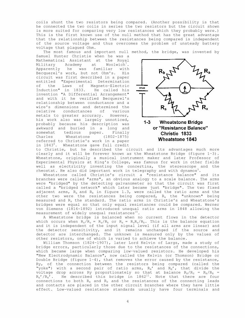
coils shunt the two resistors being compared. (Another possibility is that he connected the two coils in series the two resistors but the circuit shown is more suited for comparing very low resistances which they probably were.) This is the first known use of the null method that has the great advantage that the relationship between the resistances being compared is independent of the source voltage and thus overcomes the problem of unsteady battery voltage that plagued Ohm. The most famous and important null method, the bridge, was invented by Samuel Hunter Christie when he was a Mathematical Assistant at the Royal Military Academy at Woolwich7. Apparently he was familiar with Becquerel's work, but not Ohm's. His circuit was first described in a paper entitled "Experimental Determination of the Laws of Magneto-Electric Induction" in 1833. He called his invention "A Differential Arrangement" and with it he verified Becquerel's relationship between conductance and a wire's dimensions and determined the relative conductances of various metals to greater accuracy. However, his work also was largely unnoticed, probably because his description was awkward and buried in a long and somewhat tedious paper. Finally Charles Wheatstone (1802-1875) referred to Christie's work in a paper in 18438. Wheatstone gave full credit to Christie, but he described the circuit and its advantages much more clearly and it will be forever known as the Wheatstone Bridge (figure 1-3). Wheatstone, originally a musical instrument maker and later Professor of Experimental Physics at King's College, was famous for work in other fields well as electricity inventing the concertina, the stereoscope and the rheostat. He also did important work in telegraphy and with dynamos9. Wheatstone called Christie's circuit a "resistance balance" and its branches were called "arms", an obvious analogy to a scale balance. The arms were "bridged" by the detecting galvanometer so that the circuit was first called a "bridged network" which later became just "bridge". The two fixed adjacent arms, Ra and Rb in figure 1.3, were called the ratio arms and the other two were the resistances being compared, Rx the "unknown" being measured and Rs the standard. The ratio arms in Christie's and Wheatstone's bridges were equal so that only equal resistances could be compared. Werner von Siemens (1816-1892) introduced unequal ratio arms in 1848 allowing the measurement of widely unequal resistances10. A Wheatstone bridge is balanced when no current flows in the detector which occurs when Rx/Rs = Ra/Rb or Rx = RsRa/Rb. This is the balance equation and it is independent of the input signal level (if all arms are linear) and the detector sensitivity, and it remains unchanged if the source and detector are interchanged. The unknown is measured only by the values of other resistors, one of which is varied to achieve the balance. William Thomson (1824-1907), later Lord Kelvin of Largs, made a study of bridge errors, particularly those due to the resistances of the connections, which became large when comparing low-valued resistors. He developed his "New Electrodynamic Balance", now called the Kelvin (or Thomson) Bridge or Double Bridge (figure 1-4), that removes the error caused by the resistance, Ry, of the connection between the resistors being compared (called the “yoke") with a second pair of ratio arms, RA’ and RB’, that divide the voltage drop across Ry proportionately so that at balance RX/RS = RA/RB = RA’/RB’. He described this bridge in 186211. Note that there are four connections to both RX and RS and the resistances of the connecting leads and contacts are placed in the other circuit branches where they have little effect. Low-valued resistance standards usually have four terminals and

5

their resistance is defined as that between the connection junctions at each end. The Kelvin Bridge was the first to make such "four-terminal" connections and as a result they are sometimes referred to as "Kelvin connections". Kelvin, whose name is also given to the absolute temperature scale, was a leading scientist in many fields. He used his bridge to measure the resistivity of copper samples as a quality control tool for the Atlantic cable project. Even though his work in electrical measurements was only one of his minor achievements, he might well be called the father of precision electrical measurements. Precision was limited by the apparatus available. Many scientists

studied bridge sensitivity including Schwendler, Heaviside, Gray and Maxwell concluding that the batteries available were not capable of producing the desired power12. Measurement precision was also limited by the detecting galvanometers used. The early galvanometers were the result of work of Ampere, Schweigger, Poggendorff, Cumming and Nobili13. Kelvin's reflecting galvanometer (1858), which was invented as a telegraphy receiver, gave much greater sensitivity14. It used a small mirror as the moving element and this reflected a focused light beam onto a distant screen. The famous D'Arsonval or moving-coil galvanometer resulted from work of Kelvin and Maxwell and was popularized by Deprez and D'Arsonval in 188215. This design was used by Weston in many pointer-type ammeters and voltmeters, but reflecting galvanometers were used to get the highest sensitivity for dc null detection. Early bridges and resistance boxes were usually adjusted by means of taper pins that connected blocks of brass arranged in various "patterns" (see Part II). "Dial" bridges used rotary switches and were thus easier to adjust but usually had higher contact resistance. “Slide-wire” or “Meter” bridges, first introduced by Gustav Robert Kirchhoff (1824-1887) use a straight piece of wire, usually German silver, to form the two ratio arms, with a sliding contact making the galvanometer connection16. This made the ratio continuously adjustable and measured on a meter scale. Professor Carey Foster's method17 puts a slide wire between the standard resistance and the resistor being compared with it, see figure 1-5. Two measurements were made with the standard and unknown interchanged thus canceling the effects of extraneous resistance and voltages as long as the resistances of

the mercury cup contacts used for the connections remained constant. This provided an alternate method to the Kelvin Bridge for the precision comparison of nearly equal resistances of low value. Yet another way to compare resistors was simply to connect the two resistors being compared in series (and in series with a source voltage) so that they passed the same current and then measuring the voltage across each. Two meters could be used or a single meter could be used for both measurements. Also a differential galvanometer could be used to measure the difference in voltage if the standard resistor could be adjusted to make the voltages equal (see figure 1-2). A modification on this was the

6

Kohlrausch "Method of Overlapping Shunts" (1904)18. It used a differential galvanometer with the two coils shunting the resistors making four-terminal connections. But to avoid errors due to differences in the resistances of the two galvanometer coils, they were ingeniously interchanged in a manner that kept the connection resistances constant. The average of the two measurements could be very precise. If a potentiometer (or a precision voltage divider) and separate voltage source is used to measure the two voltages, this is called the potentiometer or “potentiometric” method19. A galvanometer null would indicate when the potentiometer voltage equaled that across each resistor. This method could give high resolution and compare resistors of widely different values, but both voltage sources had to remain very stable as the two measurements were made. Yet a better method is to connect the divider across both resistors forming a bridge and make four balances, one connecting the galvanometer to each end of each resistor. This allowed four-terminal measurements and had most of the advantages of a bridge but a more complicated calculation was required. The variety and precision of dc resistance measurements improved greatly through the last of nineteenth century and into the twentieth spurred on by corresponding improvements in the standards of resistance and the founding of the many great national standards laboratories that determined and preserved the values of the electrical units, including the Ohm. 1.2 Dc to Ac, Capacitance and Inductance Measurements While Ohm's Law originally considered only resistance, there were other quantities that affected current, at least transient current. The first capacitors, Leyden Jars, were invented by von Kleist and von Musschenbroek in the 18th century and improved capacitors were developed by others including Michael Faraday (1791-1867) who measured the "specific inductive capacity" (dielectric constant) of various insulating materials. He measured the relative capacitance of two capacitors using an early electrometer similar to Coulomb's Torsion Balance (Charles Augustin Coulomb 1736-1806) noting the relative decrease in charge of one capacitor when it charged a second capacitor. Relative capacitance was also measured by comparing the relative galvanometer deflections they gave when discharged20 Like Ohm's resistance measurements, these were "meter" methods whose accuracy depended on the linearity of the detecting charge or current sensing device and the stability of the dc source. Faraday and Joseph Henry (1797-1878) independently discovered mutual inductance in 1831 and self-inductance in 1832 with Faraday getting most of the credit for the former and Henry for the latter21. They measured relative inductance values by meter deflection methods. In 1852 R. Felici demonstrated mutual induction in the simple null circuit of figure 1.6 that compared a fixed inductor against a variable one. Although this was actually not a bridge, it is perhaps the first ballistic (transient) null method and thus an important step22. Much later (1882) Heaviside used this simple circuit with a telephone as detector. James Clerk Maxwell (1831-1879) introduced a ballistic deflection method for measuring inductance and resistance in 186523, see figure 1-7. This bridge was first balanced as a Wheatstone bridge with a steady dc applied. Then the battery connection was opened or closed to give an inductive transient. The inductance then could be calculated from the magnitude of the transient galvanometer deflection and the galvanometer's ballistic (impulse) calibration. Thus this was a combined bridge-meter method, a bridge for resistance and a meter for inductance.

7

If an adjustment is made to null this transient deflection, the circuit becomes a "ballistic bridge". While Maxwell introduced ballistic bridges for inductance measurements (see below) the first such bridge may have been one by C. V. de Sauty (who worked on the Atlantic cable, as did Kelvin) in (or before) 1871 that he used for capacitance measurements figure 1-8. Here the capacitance ratio is measured in terms of the resistance ratio when the transient is nulled by making the RC time constants equal24. Because of this method, bridges that compare the ratio of two capacitors to the ratio of two resistors are often called de Sauty bridges. Several other researchers made null measurements to compare capacitance ratios to resistance ratios, but unlike de Sauty's circuit that switched only the input, they used switches in the circuit itself that were depressed in a certain sequence. In Thomson's (Kelvin's) "method of mixtures", figure 1-9, (1873) switches S1 and S2 were closed to charge the two capacitors to voltages, V1 and V2, proportional to the resistor ratio. Then these switches were opened and S3 closed so that the charges on the two capacitors “mix” (positive charge in CS flows into CX). If the charges on the two capacitors had been equal, Q1 = C1V1 = C2V2 = Q2, the discharge would be complete and there would be no transient on the galvanometer when S4 is closed15. The circuit by J. Gott in figure 1-10 (1881) looks even more like a bridge26. He charged the

8

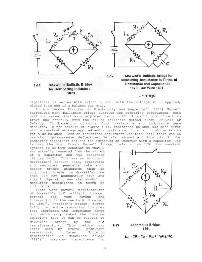
capacitors is series with switch S1 and, with the voltage still applied, closed S2 to see if a balance was made. In his famous Treatise on Electricity and Magnetism27 (1873) Maxwell introduced many ballistic bridge circuits for comparing inductances, both self and mutual that were adjusted for a null. It would be difficult to prove who actually used the nulled ballistic method first, Maxwell or DeSauty. In Maxwell's circuits, both resistance and inductance were measured. In the circuit of figure 1-11, resistance balance was made first with a constant voltage applied and a resistance, r, added to either arm to get a dc balance. Then an inductance adjustment was made until there was no transient galvanometer deflection. He also showed a bridge circuit for comparing capacitors and one for comparing an inductor with a capacitor. The latter, the most famous Maxwell Bridge, balanced an L/R time constant against an RC time constant so that L was actually measured from the values of a capacitor and two resistors (figure 1-12). This was an important development because today capacitors and resistors generally make much better bridge standards than do inductors. However in Maxwell’s time this was not necessarily true and this bridge might was also useful in measuring capacitance in terms of inductance. There were several modifications of Maxwell's L-C ballistic bridge, perhaps the most famous and interesting is the one by A. Anderson in 189128. Anderson's bridge, figure 1-13, had extra resistive branches that increased its inductance range but which complicated the balance equations (but it can be reduced to Maxwell's bridge by the Y-∆ transformation). This bridge was later used by several prominent researchers. Carey Foster’s modification of Maxwell’s bridge (1887)29 compared capacitance to

9

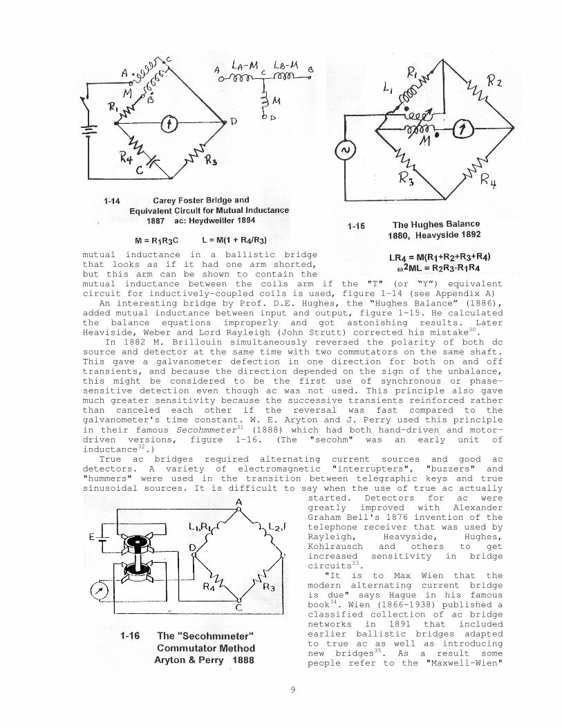
mutual inductance in a ballistic bridge that looks as if it had one arm shorted, but this arm can be shown to contain the mutual inductance between the coils arm if the "T" (or “Y”) equivalent circuit for inductively-coupled coils is used, figure 1-14 (see Appendix A) An interesting bridge by Prof. D.E. Hughes, the “Hughes Balance” (1886), added mutual inductance between input and output, figure 1-15. He calculated the balance equations improperly and got astonishing results. Later Heaviside, Weber and Lord Rayleigh (John Strutt) corrected his mistake30. In 1882 M. Brillouin simultaneously reversed the polarity of both dc source and detector at the same time with two commutators on the same shaft. This gave a galvanometer defection in one direction for both on and off transients, and because the direction depended on the sign of the unbalance, this might be considered to be the first use of synchronous or phase-sensitive detection even though ac was not used. This principle also gave much greater sensitivity because the successive transients reinforced rather than canceled each other if the reversal was fast compared to the galvanometer's time constant. W. E. Aryton and J. Perry used this principle in their famous Secohmmeter31 (1888) which had both hand-driven and motor-driven versions, figure 1-16. (The "secohm" was an early unit of inductance32.) True ac bridges required alternating current sources and good ac detectors. A variety of electromagnetic "interrupters", "buzzers" and "hummers" were used in the transition between telegraphic keys and true sinusoidal sources. It is difficult to say when the use of true ac actually

started. Detectors for ac were greatly improved with Alexander Graham Bell's 1876 invention of the telephone receiver that was used by Rayleigh, Heavyside, Hughes, Kohlrausch and others to get increased sensitivity in bridge circuits33. "It is to Max Wien that the modern alternating current bridge is due" says Hague in his famous book34. Wien (1866-1938) published a classified collection of ac bridge networks in 1891 that included earlier ballistic bridges adapted to true ac as well as introducing new bridges35. As a result some people refer to the "Maxwell-Wien"

10

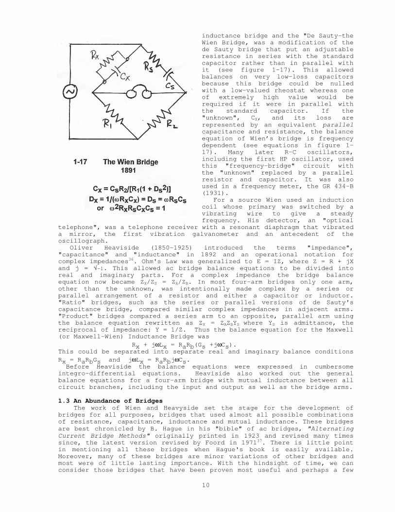
inductance bridge and the "De Sauty-the Wien Bridge, was a modification of the de Sauty bridge that put an adjustable resistance in series with the standard capacitor rather than in parallel with it (see figure 1-17). This allowed balances on very low-loss capacitors because this bridge could be nulled with a low-valued rheostat whereas one of extremely high value would be required if it were in parallel with the standard capacitor. If the "unknown", CX, and its loss are represented by an equivalent parallel capacitance and resistance, the balance equation of Wien’s bridge is frequency dependent (see equations in figure 1-17). Many later R-C oscillators, including the first HP oscillator, used this "frequency-bridge" circuit with the "unknown" replaced by a parallel resistor and capacitor. It was also used in a frequency meter, the GR 434-B (1931). For a source Wien used an induction coil whose primary was switched by a vibrating wire to give a steady frequency. His detector, an "optical

telephone", was a telephone receiver with a resonant diaphragm that vibrated a mirror, the first vibration galvanometer and an antecedent of the oscillograph. Oliver Heaviside (1850-1925) introduced the terms "impedance", "capacitance" and "inductance" in 1892 and an operational notation for complex impedances36. Ohm's Law was generalized to E = IZ, where Z = R + jX and j = �-1. This allowed ac bridge balance equations to be divided into real and imaginary parts. For a complex impedance the bridge balance equation now became ZX/ZS = ZA/ZB. In most four-arm bridges only one arm, other than the unknown, was intentionally made complex by a series or parallel arrangement of a resistor and either a capacitor or inductor. "Ratio" bridges, such as the series or parallel versions of de Sauty's capacitance bridge, compared similar complex impedances in adjacent arms. "Product" bridges compared a series arm to an opposite, parallel arm using the balance equation rewritten as ZX = ZAZBYS where YS is admittance, the reciprocal of impedance: Y = 1/Z. Thus the balance equation for the Maxwell (or Maxwell-Wien) Inductance Bridge was Rx + jωLx = RaRb(Gs +jωCs). This could be separated into separate real and imaginary balance conditions Rx = RaRbGs and jωLx = RaRbjωCs. Before Heaviside the balance equations were expressed in cumbersome integro-differential equations. Heaviside also worked out the general balance equations for a four-arm bridge with mutual inductance between all circuit branches, including the input and output as well as the bridge arms. 1.3 An Abundance of Bridges The work of Wien and Heavyside set the stage for the development of bridges for all purposes, bridges that used almost all possible combinations of resistance, capacitance, inductance and mutual inductance. These bridges are best chronicled by B. Hague in his "bible" of ac bridges, "Alternating Current Bridge Methods" originally printed in 1923 and revised many times since, the latest version revised by Foord in 197137. There is little point in mentioning all these bridges when Hague's book is easily available. Moreover, many of these bridges are minor variations of other bridges and most were of little lasting importance. With the hindsight of time, we can consider those bridges that have been proven most useful and perhaps a few

11

others of particular historical interest. It is easiest to consider these grouped by the parameter measured. The capacitance bridge story is relatively simple. Wien added series and parallel resistances to de Sauty's bridge to allow the measurement of series or parallel capacitance, and these are the two capacitance bridges used later in most general-purpose impedance bridges, with the series bridge more important because series capacitance is usually specified for capacitors and because the parallel bridge requires a very high-valued resistor to make low D (dissipation factor, D = RX/XX) measurements. At NBS, F.W. Grover in 1907 compared an unknown capacitor against another capacitive arm with no loss adjustment and made both real and imaginary balances with a pair of inductive arms, one or both variable and in series with a variable resistor38. The two inductive arms were not coupled as in later transformer-ratio-arm bridges. Fleming and van Dyke's "Four Condenser Bridge" (1912) was a variation of the Wien bridge with capacitive ratio arms39. This allowed high-impedance ratio arms for best sensitivity when measuring small capacitances, such as samples of dielectric materials, but avoided the large phase-angle errors of high-valued resistive arms especially at higher frequencies. C.E. Hay made a capacitance version of Anderson's bridge by adding extra branches to the parallel capacitance bridge (1913)40.

More important than these variations was the Schering Bridge (figure 1-18), named for H. Schering of the PTB, the German national laboratory, who suggested the circuit in 192041 even though the same circuit was described in a U.S. Patent filed by Phillips Thomas in 191542. This bridge has several important uses. First it is an excellent bridge for low-loss measurements because the phase adjustment is a variable capacitor that can give high resolution. Second, it has had much use as a high-voltage bridge (both high-voltage ac and ac with high-voltage dc bias) because most of the ac voltage (and all of the

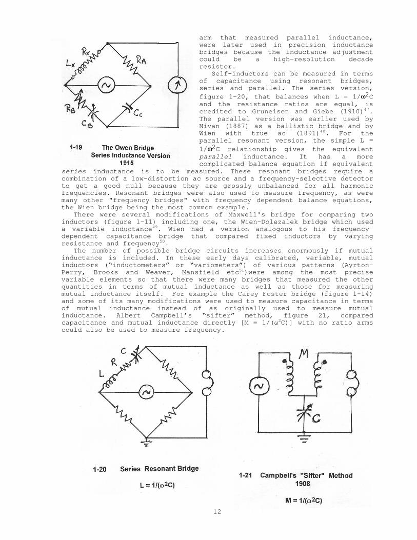
dc voltage) is applied only to the unknown and a high-voltage standard capacitor (if the resistor ratio arms are of low value). Finally it makes an excellent high-frequency bridge because both adjustments are variable capacitors that can have excellent high-frequency characteristics (see part 2.4). The self-inductance bridge story is more complicated because there are so many possible bridges that measure self-inductance in terms of a capacitance, another self-inductance or a mutual inductance. The most important bridges over time have been the Maxwell (or Maxwell-Wien) bridge, of figure 1-12 and its many variations. Anderson's ballistic bridge with its extra arm was modified for ac by Rowland (1898) and used for precision measurements by several including Rosa and Grover of NBS43. Stroud and Oates44 used it backwards (interchanging source and detector) and had that circuit named after them even though it has the same balance equations. C.E. Hay (1910) replaced the parallel R-C arm of the Maxwell Bridge with a series one45. This measured parallel inductance, but allowed measurement of higher Q values (ωL/R) without requiring a very high-valued variable resistance. The Hay bridge was also more convenient to use for measurements on inductors when they were biased by dc current because the series R-C arm blocked the flow of dc current. The Hay and Maxwell bridges were both chosen for inductance measurements in later LRC or "Universal" measuring instruments. The Owen bridge (D. Owen, 1915), figure 1-19, removed the parallel resistor of the Maxwell bridge and put instead a series capacitor in an arm adjacent to the unknown46. This circuit, and a modification of it with a parallel R-C

12

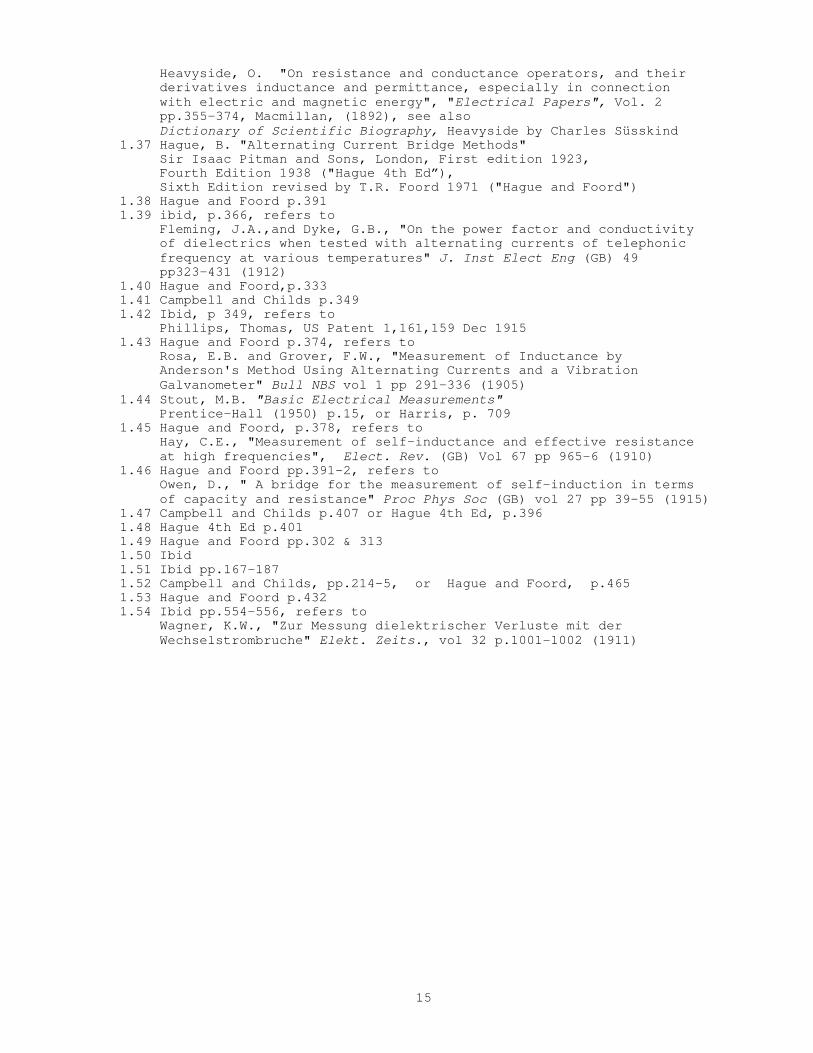
arm that measured parallel inductance, were later used in precision inductance bridges because the inductance adjustment could be a high-resolution decade resistor. Self-inductors can be measured in terms of capacitance using resonant bridges, series and parallel. The series version, figure 1-20, that balances when L = 1/ω2C and the resistance ratios are equal, is credited to Gruneisen and Giebe (1910)47. The parallel version was earlier used by Nivan (1887) as a ballistic bridge and by Wien with true ac (1891)48. For the parallel resonant version, the simple L = 1/ω2C relationship gives the equivalent parallel inductance. It has a more complicated balance equation if equivalent

series inductance is to be measured. These resonant bridges require a combination of a low-distortion ac source and a frequency-selective detector to get a good null because they are grossly unbalanced for all harmonic frequencies. Resonant bridges were also used to measure frequency, as were many other "frequency bridges" with frequency dependent balance equations, the Wien bridge being the most common example. There were several modifications of Maxwell's bridge for comparing two inductors (figure 1-11) including one, the Wien-Dolezalek bridge which used a variable inductance49. Wien had a version analogous to his frequency-dependent capacitance bridge that compared fixed inductors by varying resistance and frequency50. The number of possible bridge circuits increases enormously if mutual inductance is included. In these early days calibrated, variable, mutual inductors (“inductometers” or “variometers”) of various patterns (Ayrton-Perry, Brooks and Weaver, Mansfield etc51)were among the most precise variable elements so that there were many bridges that measured the other quantities in terms of mutual inductance as well as those for measuring mutual inductance itself. For example the Carey Foster bridge (figure 1-14) and some of its many modifications were used to measure capacitance in terms of mutual inductance instead of as originally used to measure mutual inductance. Albert Campbell’s “sifter” method, figure 21, compared capacitance and mutual inductance directly [M = 1/(�2C)] with no ratio arms could also be used to measure frequency.

13

The Maxwell-Wien bridge of figure 1-22 was used for comparing the mutual inductance of a pair of coils to the self-inductance of one of them. (Its balance equation is easily derived using the equivalent circuit of figure 1-14). It had many modifications (Campbell, Heavyside, and Butterworth) and there were many modifications of these modifications53. Most of these had complicated, frequency-dependent balance equations and we might wonder now if all these bridges were really of much practical use.

Karl Wagner made an important contribution to bridge measurements when he introduced the "Wagner Ground" (or “Wagner Earth”) in 1911 (figure 1-23). Wagner used these auxiliary bridge arms (C1 and C2) to remove the effect of the capacitance between the observer's hand and the detector54. More generally it can be used to make guarded, three-terminal measurements such as those on shielded three-terminal capacitors as shown in the figure. Balances are made with the switch in both positions. When the auxiliary arm, C2, is adjusted so that the point P is at ground potential, Cb has no effect and Cx is measured directly. This auxiliary circuit was later used in commercial capacitance bridges and resistive Wagner balances are used to guard out leakage resistance to ground in dc high-resistance bridges. It is interesting to note that a resistance bridge with a Wagner balance is the topological dual of the Kelvin bridge (figure 1-4) which also has two auxiliary arms and requires two balance adjustments.

14

References Part I 8/7/07 1.1 Bordeau, Sanford P. , "Volts to Hertz" Burgess Pub Co. p. 91 1.2 Keithley, Joseph F.,“The Story of Electrical and Magnetic Measurements” IEEE Press (1999), p. 95 1.3 Bordeau p.100 1.4 Encyclopedia Brtiannica, "Ohm" 1.5 Drysdale and Jolley, "Electrical Measuring Instruments" Ernest Benn Ltd. London 1924, Vol 1, p.142 1.6 Dictionary of Scientific Biography, Becquerel, A.C. by David M. Knight 1.7 Dictionary of Scientific Biography, Christie, S.H. by Edgar W. Morse 1.8 Hague, B. and Foord, T.R., “Alternating Current Bridge Methods, 6th edition, Pitman Publishing 1971, p.2 1.9 Dictionary of Scientific Biography, Wheatstone by Sigalia Dostrovsky 1.10 Hague and Foord, pp.3-4 1.11 Wenner F. "Methods, Apparatus, and Procedure for the Comparison of Precision Standard Resistors" NBS Research Paper RP1323 NBS Jour. of Research, Vol 25, Aug 1940, p. 231 1.12 ibid 1.13 Keithley, p.75 1.14 Laws, F.A., "Electrical Measurements" McGraw-Hill Book Co. (1917), p.5, refers to Ewing, J.A., "The Work of Lord Kelvin in Telegraphy and Navigation" Jour Inst of Elect Engrs (GB) vol.44, 1910 p.538 1.15 Laws p.32 1.16 Gray, A., "Absolute Measurements in Electricity and Magnetism" MacMillan, 2nd Ed 1921 p.142 1.17 Laws, p.175 1.18 Laws, p. 159, also Thomas, J.L., “Precision Resistors and Their Measurement”, p13, NBS Circular 470 and Kohlrausch, F., Wied. Ann.20,76 (1883). 1.19 Harris, Forset K., “Electrical Measurements” John Wiley & Sons, 1959, p. 257 1.20 Gray, p.721 1.21 Bordeau, p.159 1.22 Hague and Foord, p.422, refers to Felici, R., "Memoire sur l'induction electrodynamiqe," Ann Chimie Phys (France) vol 34, 3rd series, pp64-77 (1852) 1.23 Hague and Foord, p.4 1.24 Hague and Foord, p.316, refers to Clark, L. and Sabine, R., "Electrical Tables and Formulae ", p.62 London, Spon (1871) 1.25 Campbell, M.A. and Childs, E.C., "Measurements of Inductance, Capacitance and Frequency," Van Nostrand 1935, p.342, refers to Thomson, W. (Lord Kelvin), Soc Tel Eng J. vol 1, p397 (1873) 1.26 Ibid p344 1.27 Maxwell, James Clark "A Treatise on Electricity and Magnetism" 1st Edition, Oxford Univ Press (1873) 1.28 Hague and Foord, pp.371-2 1.29 Hague and Foord, p.455 1.30 Ibid p451 1.31 Hague & Foord p.5, refers to Ayrton, W.E., and Perry, J., “Modes of measuring the coefficients of Self and murual induction,” J. Soc. Telegr. Engrs (GB), vol. 16 pp.292-343, (1888), also see Milner, S.R., "On the use of the Secohmmeter for the Measurement of Combined Resistances and Capacities" Phil. Mag. vol 12, 1906 p.297 1.32 Drysdale and Jolley vol 1, p.131 1.33 Hague and Foord, p.5 1.34 Ibid 1.35 Ibid p.5, refers to Wien, M. “Das Tetephon als optischer Apparat zur Strommessung” 1.36 Hague, Fourth Ed p.33, refers to

15

Heavyside, O. "On resistance and conductance operators, and their derivatives inductance and permittance, especially in connection with electric and magnetic energy", "Electrical Papers", Vol. 2 pp.355-374, Macmillan, (1892), see also Dictionary of Scientific Biography, Heavyside by Charles Süsskind 1.37 Hague, B. "Alternating Current Bridge Methods" Sir Isaac Pitman and Sons, London, First edition 1923, Fourth Edition 1938 ("Hague 4th Ed”), Sixth Edition revised by T.R. Foord 1971 ("Hague and Foord") 1.38 Hague and Foord p.391 1.39 ibid, p.366, refers to Fleming, J.A.,and Dyke, G.B., "On the power factor and conductivity of dielectrics when tested with alternating currents of telephonic frequency at various temperatures" J. Inst Elect Eng (GB) 49 pp323-431 (1912) 1.40 Hague and Foord,p.333 1.41 Campbell and Childs p.349 1.42 Ibid, p 349, refers to Phillips, Thomas, US Patent 1,161,159 Dec 1915 1.43 Hague and Foord p.374, refers to Rosa, E.B. and Grover, F.W., "Measurement of Inductance by Anderson's Method Using Alternating Currents and a Vibration Galvanometer" Bull NBS vol 1 pp 291-336 (1905) 1.44 Stout, M.B. "Basic Electrical Measurements" Prentice-Hall (1950) p.15, or Harris, p. 709 1.45 Hague and Foord, p.378, refers to Hay, C.E., "Measurement of self-inductance and effective resistance at high frequencies", Elect. Rev. (GB) Vol 67 pp 965-6 (1910) 1.46 Hague and Foord pp.391-2, refers to Owen, D., " A bridge for the measurement of self-induction in terms of capacity and resistance" Proc Phys Soc (GB) vol 27 pp 39-55 (1915) 1.47 Campbell and Childs p.407 or Hague 4th Ed, p.396 1.48 Hague 4th Ed p.401 1.49 Hague and Foord pp.302 & 313 1.50 Ibid 1.51 Ibid pp.167-187 1.52 Campbell and Childs, pp.214-5, or Hague and Foord, p.465 1.53 Hague and Foord p.432 1.54 Ibid pp.554-556, refers to Wagner, K.W., "Zur Messung dielektrischer Verluste mit der Wechselstrombruche" Elekt. Zeits., vol 32 p.1001-1002 (1911)